Page 1
Date of issue: Sept. 28, 2011 Project: SKA Spectrum Monit., RM
Revision nr.: 1.0 Authors: A.J. Boonstra and R.P. MillenaarStatus: Final Kind of issue: Limited
SKA Site Spectrum Monitoring
Sites: X1 - X4 and Y1 - Y4
Measurement Mode: Rural Mode (RM)
Annex to the report
”SKA site spectrum monitoring, measurement program and data processing”
Verified:
Name Signature Date Rev.nr.
... 1.0
Accepted:
R.P. Millenaar R.T. Schilizzi
.................. .................. ..................
date: date: date:
c©ASTRON 2011
1
Page 2
Date of issue: Sept. 28, 2011 Project: SKA Spectrum Monit., RM
Revision nr.: 1.0 Authors: A.J. Boonstra and R.P. MillenaarStatus: Final Kind of issue: Limited
Distribution list:
Group: For Information:
Expert Panel on RFI and EMI R.T. Schilizzi
Document revision:
Revision Date Section Page(s) Modification
1.0 Sept. 28, 2011 all all creation
2
Page 3
Date of issue: Sept. 28, 2011 Project: SKA Spectrum Monit., RM
Revision nr.: 1.0 Authors: A.J. Boonstra and R.P. MillenaarStatus: Final Kind of issue: Limited
Contents
1 Introduction 4
2 Measurement results 5
2.1 Spectral power flux density results, overview . . . . . . . . . . . . . . . . . . . . . . . . . . 7
2.2 Spectral power flux density results, expanded scales . . . . . . . . . . . . . . . . . . . . . 11
2.2.1 Spectral power flux density, sites X1 and Y1 . . . . . . . . . . . . . . . . . . . . . 12
2.2.2 Spectral power flux density, sites X2 and Y2 . . . . . . . . . . . . . . . . . . . . . 23
2.2.3 Spectral power flux density, sites X3 and Y3 . . . . . . . . . . . . . . . . . . . . . 34
2.2.4 Spectral power flux density, sites X4 and Y4 . . . . . . . . . . . . . . . . . . . . . 45
2.3 Sensitivity . . . . . . . . . . . . . . . . . . . . . . . . . . . . . . . . . . . . . . . . . . . . . 56
Appendix A. Calibration results 58
A1. Gain . . . . . . . . . . . . . . . . . . . . . . . . . . . . . . . . . . . . . . . . . . . . . . . . 59
A2. Receiver and system temperature . . . . . . . . . . . . . . . . . . . . . . . . . . . . . . . . 60
A3. Calibrated spectra, all sites . . . . . . . . . . . . . . . . . . . . . . . . . . . . . . . . . . . . 62
A4. Calibrated spectra, percentiles . . . . . . . . . . . . . . . . . . . . . . . . . . . . . . . . . . 63
3
Page 4
Date of issue: Sept. 28, 2011 Project: SKA Spectrum Monit., RM
Revision nr.: 1.0 Authors: A.J. Boonstra and R.P. MillenaarStatus: Final Kind of issue: Limited
1 Introduction
As part of the SKA site selection process the Radio Frequency Interference environment has been mea-
sured at the candidate sites X and Y. This was done under the “Agreement on radio frequency interference
monitoring 2008”. This Agreement entails the development of instrumentation, control and data pro-
cessing software, infrastructure and carrying out of measurements at the two candidate core sites, plus
at a selection of remote sites in the hosts proposed array configuration. This spectrum monitoring report
is one of a series and is annex to the report “SKA site spectrum monitoring, measurement program and
data processing”. The results of complete Rural Mode (RM) runs are presented for four remote sites
at each of the two candidate SKA hosting countries, respectively X1, X2, X3, X4, Y1, Y2, Y3, and Y4.
This measurement annex report presents the following:
• calibrated and baseline corrected overview spectra for the frequency range 70-2000 MHz in section
2.1.,
• 200 MHz wide zoomed-in spectra in section 2.2.,
• sensitivity spectra in section 2.3..
In order to help judging the validity of the data, calibration results are included in appendix A:
• calibrated gain curves in appendix A1,
• calibrated Trec and Tsys curves in appendix A2,
• calibrated site-overview spectra without “baseline correction” in appendix A3,
• calibrated percentile spectra without “baseline correction” in appendix A4.
The Rural Mode measurement uses the following settings:
• integration time: 60 s (per spectrum)
• number of repetitions: 10
• net integration time per pointing/polarisation/band: 600 seconds (10 minutes)
• calibration: equal time on noise source on/off/antenna (60s/60s/60s), each repetition.
A complete scan (1 pointing, 1 polarisation, 9 bands), including calibration and overhead, takes a total
of about 5.8 hours. For a complete survey, all pointings and polarisations, a total of about 2 days was
required.
This report does not contain detailed descriptions of the presented results as these are included in the
main report mentioned above. The basic information is present in the figure captions, for more details
please see the main report.
4
Page 5
Date of issue: Sept. 28, 2011 Project: SKA Spectrum Monit., RM
Revision nr.: 1.0 Authors: A.J. Boonstra and R.P. MillenaarStatus: Final Kind of issue: Limited
2 Measurement results
5
Page 6
Date of issue: Sept. 28, 2011 Project: SKA Spectrum Monit., RM
Revision nr.: 1.0 Authors: A.J. Boonstra and R.P. MillenaarStatus: Final Kind of issue: Limited
The figures that follow result from observations at locations X1-4 and Y1-4; these figures for sites X and
Y are combined when displayed on each page. This may suggest that site X1 is to be compared with site
Y1 and so on. This however is not the case: in fact the sites identified by the numbers 1 to 4 are selected
without having a particular order in mind. The selection of the four sites at each of the two countries
was done to include expected noisy and relatively quiet locations from the set of 25 remote station sites.
Concerning the quality of the data please note that the gain settings of the equipment was adapted by
adding an additional attenuator. This was done to improve the dynamic range of the monitoring systems
at all 2 × 4 sites, some of which may be near to strong transmitters. This additional attenuaton led to
a lower noise source calibration signal power. Together with (relatively) strong interference this has led
to distorted calibration of part of the data. This effect can be seen in the calibration curves, but also in
some cases as distorted (baseline) curves for median Ψ and Ψc data.
For the data at hand, no detection was done on self-generated RFI. When inspecting the data, care nust
be taken not to confuse self-gerated RFI from “real” external RFI. Known issues are mid-band narrow
RFI spikes (visible in the receiver noise temperature calibration curves) which may occur at 243.770,
719.985, 975.020, 1218.765, 1452.488, 1679.985, and 1912.513 MHz.
Another artefact is apparent RFI in baseline-calibrated data Ψc stemming from false detection of RFI at
frequency band transitions. This kind of self-generated RFI may occur at the band edges at 190, 440, 540,
855, 1080, 1340, 1595, and / or 1780 MHz. At these frequencies the calibrated non-baseline subtracted
data Ψ in some cases show jumps in the calibrated spectra. Comparing the Ψc and Ψ (Matlab fig-file)
data will show whether a spike in Ψc data at a band edge is an artefact or not.
6
Page 7
Date of issue: Sept. 28, 2011 Project: SKA Spectrum Monit., RM
Revision nr.: 1.0 Authors: A.J. Boonstra and R.P. MillenaarStatus: Final Kind of issue: Limited
2.1 Spectral power flux density results, overview
Figure 1: Calibrated and baseline-corrected power flux density Ψc in dB(Wm−2Hz−1). Plotted are the 50 (median),
75, an 95 percentile curves, which were computed from datasets obtained in four azimuth directions (North, South,
East and West) and for two polarizations (horizontal and vertical). The 1 σ level is shown in black; the actual
detection level for the baseline subtraction procedure is 6 σ.
7
Page 8
Date of issue: Sept. 28, 2011 Project: SKA Spectrum Monit., RM
Revision nr.: 1.0 Authors: A.J. Boonstra and R.P. MillenaarStatus: Final Kind of issue: Limited
Figure 2: Calibrated and baseline-corrected power flux density Ψc in dB(Wm−2Hz−1). Plotted are the 50 (median),
75, an 95 percentile curves, which were computed from datasets obtained in four azimuth directions (North, South,
East and West) and for two polarizations (horizontal and vertical). The 1 σ level is shown in black; the actual
detection level for the baseline subtraction procedure is 6 σ.
8
Page 9
Date of issue: Sept. 28, 2011 Project: SKA Spectrum Monit., RM
Revision nr.: 1.0 Authors: A.J. Boonstra and R.P. MillenaarStatus: Final Kind of issue: Limited
Figure 3: Calibrated and baseline-corrected power flux density Ψc in dB(Wm−2Hz−1). Plotted are the 50 (median),
75, an 95 percentile curves, which were computed from datasets obtained in four azimuth directions (North, South,
East and West) and for two polarizations (horizontal and vertical). The 1 σ level is shown in black; the actual
detection level for the baseline subtraction procedure is 6 σ.
9
Page 10
Date of issue: Sept. 28, 2011 Project: SKA Spectrum Monit., RM
Revision nr.: 1.0 Authors: A.J. Boonstra and R.P. MillenaarStatus: Final Kind of issue: Limited
Figure 4: Calibrated and baseline-corrected power flux density Ψc in dB(Wm−2Hz−1). Plotted are the 50 (median),
75, an 95 percentile curves, which were computed from datasets obtained in four azimuth directions (North, South,
East and West) and for two polarizations (horizontal and vertical). The 1 σ level is shown in black; the actual
detection level for the baseline subtraction procedure is 6 σ.
10
Page 11
Date of issue: Sept. 28, 2011 Project: SKA Spectrum Monit., RM
Revision nr.: 1.0 Authors: A.J. Boonstra and R.P. MillenaarStatus: Final Kind of issue: Limited
2.2 Spectral power flux density results, expanded scales
11
Page 12
Date of issue: Sept. 28, 2011 Project: SKA Spectrum Monit., RM
Revision nr.: 1.0 Authors: A.J. Boonstra and R.P. MillenaarStatus: Final Kind of issue: Limited
2.2.1 Spectral power flux density, sites X1 and Y1
12
Page 13
Date of issue: Sept. 28, 2011 Project: SKA Spectrum Monit., RM
Revision nr.: 1.0 Authors: A.J. Boonstra and R.P. MillenaarStatus: Final Kind of issue: Limited
Figure 5: Calibrated and baseline-corrected power flux density Ψc in dB(Wm−2Hz−1) using expanded frequency
scaling. Plotted are the 50 (median), 75, an 95 percentile curves, which were computed from datasets obtained in
four azimuth directions (North, South, East and West) and for two polarizations (horizontal and vertical). The 1
σ level is shown in black; the actual detection level for the baseline subtraction procedure is 6 σ.
13
Page 14
Date of issue: Sept. 28, 2011 Project: SKA Spectrum Monit., RM
Revision nr.: 1.0 Authors: A.J. Boonstra and R.P. MillenaarStatus: Final Kind of issue: Limited
Figure 6: Calibrated and baseline-corrected power flux density Ψc in dB(Wm−2Hz−1) using expanded frequency
scaling. Plotted are the 50 (median), 75, an 95 percentile curves, which were computed from datasets obtained in
four azimuth directions (North, South, East and West) and for two polarizations (horizontal and vertical). The 1
σ level is shown in black; the actual detection level for the baseline subtraction procedure is 6 σ.
14
Page 15
Date of issue: Sept. 28, 2011 Project: SKA Spectrum Monit., RM
Revision nr.: 1.0 Authors: A.J. Boonstra and R.P. MillenaarStatus: Final Kind of issue: Limited
Figure 7: Calibrated and baseline-corrected power flux density Ψc in dB(Wm−2Hz−1) using expanded frequency
scaling. Plotted are the 50 (median), 75, an 95 percentile curves, which were computed from datasets obtained in
four azimuth directions (North, South, East and West) and for two polarizations (horizontal and vertical). The 1
σ level is shown in black; the actual detection level for the baseline subtraction procedure is 6 σ.
15
Page 16
Date of issue: Sept. 28, 2011 Project: SKA Spectrum Monit., RM
Revision nr.: 1.0 Authors: A.J. Boonstra and R.P. MillenaarStatus: Final Kind of issue: Limited
Figure 8: Calibrated and baseline-corrected power flux density Ψc in dB(Wm−2Hz−1) using expanded frequency
scaling. Plotted are the 50 (median), 75, an 95 percentile curves, which were computed from datasets obtained in
four azimuth directions (North, South, East and West) and for two polarizations (horizontal and vertical). The 1
σ level is shown in black; the actual detection level for the baseline subtraction procedure is 6 σ.
16
Page 17
Date of issue: Sept. 28, 2011 Project: SKA Spectrum Monit., RM
Revision nr.: 1.0 Authors: A.J. Boonstra and R.P. MillenaarStatus: Final Kind of issue: Limited
Figure 9: Calibrated and baseline-corrected power flux density Ψc in dB(Wm−2Hz−1) using expanded frequency
scaling. Plotted are the 50 (median), 75, an 95 percentile curves, which were computed from datasets obtained in
four azimuth directions (North, South, East and West) and for two polarizations (horizontal and vertical). The 1
σ level is shown in black; the actual detection level for the baseline subtraction procedure is 6 σ.
17
Page 18
Date of issue: Sept. 28, 2011 Project: SKA Spectrum Monit., RM
Revision nr.: 1.0 Authors: A.J. Boonstra and R.P. MillenaarStatus: Final Kind of issue: Limited
Figure 10: Calibrated and baseline-corrected power flux density Ψc in dB(Wm−2Hz−1) using expanded frequency
scaling. Plotted are the 50 (median), 75, an 95 percentile curves, which were computed from datasets obtained in
four azimuth directions (North, South, East and West) and for two polarizations (horizontal and vertical). The 1
σ level is shown in black; the actual detection level for the baseline subtraction procedure is 6 σ.
18
Page 19
Date of issue: Sept. 28, 2011 Project: SKA Spectrum Monit., RM
Revision nr.: 1.0 Authors: A.J. Boonstra and R.P. MillenaarStatus: Final Kind of issue: Limited
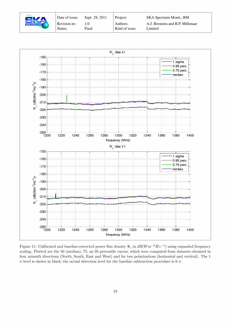
Figure 11: Calibrated and baseline-corrected power flux density Ψc in dB(Wm−2Hz−1) using expanded frequency
scaling. Plotted are the 50 (median), 75, an 95 percentile curves, which were computed from datasets obtained in
four azimuth directions (North, South, East and West) and for two polarizations (horizontal and vertical). The 1
σ level is shown in black; the actual detection level for the baseline subtraction procedure is 6 σ.
19
Page 20
Date of issue: Sept. 28, 2011 Project: SKA Spectrum Monit., RM
Revision nr.: 1.0 Authors: A.J. Boonstra and R.P. MillenaarStatus: Final Kind of issue: Limited
Figure 12: Calibrated and baseline-corrected power flux density Ψc in dB(Wm−2Hz−1) using expanded frequency
scaling. Plotted are the 50 (median), 75, an 95 percentile curves, which were computed from datasets obtained in
four azimuth directions (North, South, East and West) and for two polarizations (horizontal and vertical). The 1
σ level is shown in black; the actual detection level for the baseline subtraction procedure is 6 σ.
20
Page 21
Date of issue: Sept. 28, 2011 Project: SKA Spectrum Monit., RM
Revision nr.: 1.0 Authors: A.J. Boonstra and R.P. MillenaarStatus: Final Kind of issue: Limited
Figure 13: Calibrated and baseline-corrected power flux density Ψc in dB(Wm−2Hz−1) using expanded frequency
scaling. Plotted are the 50 (median), 75, an 95 percentile curves, which were computed from datasets obtained in
four azimuth directions (North, South, East and West) and for two polarizations (horizontal and vertical). The 1
σ level is shown in black; the actual detection level for the baseline subtraction procedure is 6 σ.
21
Page 22
Date of issue: Sept. 28, 2011 Project: SKA Spectrum Monit., RM
Revision nr.: 1.0 Authors: A.J. Boonstra and R.P. MillenaarStatus: Final Kind of issue: Limited
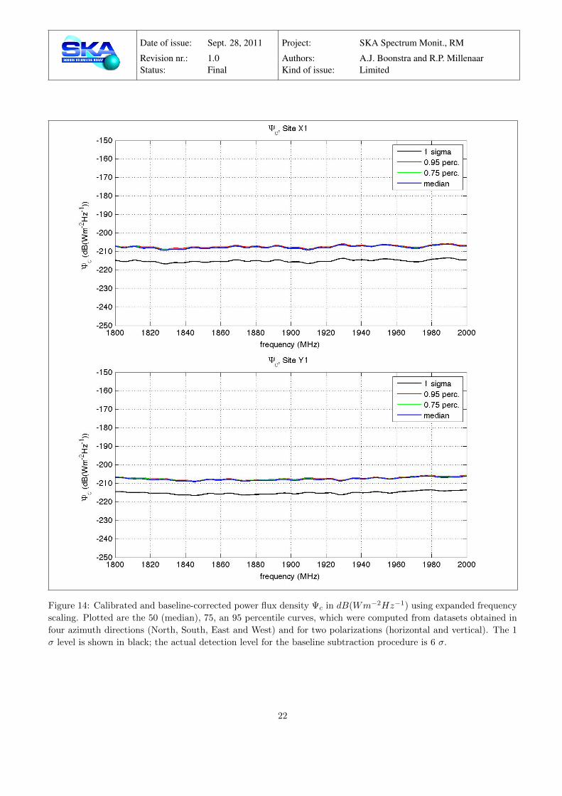
Figure 14: Calibrated and baseline-corrected power flux density Ψc in dB(Wm−2Hz−1) using expanded frequency
scaling. Plotted are the 50 (median), 75, an 95 percentile curves, which were computed from datasets obtained in
four azimuth directions (North, South, East and West) and for two polarizations (horizontal and vertical). The 1
σ level is shown in black; the actual detection level for the baseline subtraction procedure is 6 σ.
22
Page 23
Date of issue: Sept. 28, 2011 Project: SKA Spectrum Monit., RM
Revision nr.: 1.0 Authors: A.J. Boonstra and R.P. MillenaarStatus: Final Kind of issue: Limited
2.2.2 Spectral power flux density, sites X2 and Y2
23
Page 24
Date of issue: Sept. 28, 2011 Project: SKA Spectrum Monit., RM
Revision nr.: 1.0 Authors: A.J. Boonstra and R.P. MillenaarStatus: Final Kind of issue: Limited
Figure 15: Calibrated and baseline-corrected power flux density Ψc in dB(Wm−2Hz−1) using expanded frequency
scaling. Plotted are the 50 (median), 75, an 95 percentile curves, which were computed from datasets obtained in
four azimuth directions (North, South, East and West) and for two polarizations (horizontal and vertical). The 1
σ level is shown in black; the actual detection level for the baseline subtraction procedure is 6 σ.
24
Page 25
Date of issue: Sept. 28, 2011 Project: SKA Spectrum Monit., RM
Revision nr.: 1.0 Authors: A.J. Boonstra and R.P. MillenaarStatus: Final Kind of issue: Limited
Figure 16: Calibrated and baseline-corrected power flux density Ψc in dB(Wm−2Hz−1) using expanded frequency
scaling. Plotted are the 50 (median), 75, an 95 percentile curves, which were computed from datasets obtained in
four azimuth directions (North, South, East and West) and for two polarizations (horizontal and vertical). The 1
σ level is shown in black; the actual detection level for the baseline subtraction procedure is 6 σ.
25
Page 26
Date of issue: Sept. 28, 2011 Project: SKA Spectrum Monit., RM
Revision nr.: 1.0 Authors: A.J. Boonstra and R.P. MillenaarStatus: Final Kind of issue: Limited
Figure 17: Calibrated and baseline-corrected power flux density Ψc in dB(Wm−2Hz−1) using expanded frequency
scaling. Plotted are the 50 (median), 75, an 95 percentile curves, which were computed from datasets obtained in
four azimuth directions (North, South, East and West) and for two polarizations (horizontal and vertical). The 1
σ level is shown in black; the actual detection level for the baseline subtraction procedure is 6 σ.
26
Page 27
Date of issue: Sept. 28, 2011 Project: SKA Spectrum Monit., RM
Revision nr.: 1.0 Authors: A.J. Boonstra and R.P. MillenaarStatus: Final Kind of issue: Limited
Figure 18: Calibrated and baseline-corrected power flux density Ψc in dB(Wm−2Hz−1) using expanded frequency
scaling. Plotted are the 50 (median), 75, an 95 percentile curves, which were computed from datasets obtained in
four azimuth directions (North, South, East and West) and for two polarizations (horizontal and vertical). The 1
σ level is shown in black; the actual detection level for the baseline subtraction procedure is 6 σ.
27
Page 28
Date of issue: Sept. 28, 2011 Project: SKA Spectrum Monit., RM
Revision nr.: 1.0 Authors: A.J. Boonstra and R.P. MillenaarStatus: Final Kind of issue: Limited
Figure 19: Calibrated and baseline-corrected power flux density Ψc in dB(Wm−2Hz−1) using expanded frequency
scaling. Plotted are the 50 (median), 75, an 95 percentile curves, which were computed from datasets obtained in
four azimuth directions (North, South, East and West) and for two polarizations (horizontal and vertical). The 1
σ level is shown in black; the actual detection level for the baseline subtraction procedure is 6 σ.
28
Page 29
Date of issue: Sept. 28, 2011 Project: SKA Spectrum Monit., RM
Revision nr.: 1.0 Authors: A.J. Boonstra and R.P. MillenaarStatus: Final Kind of issue: Limited
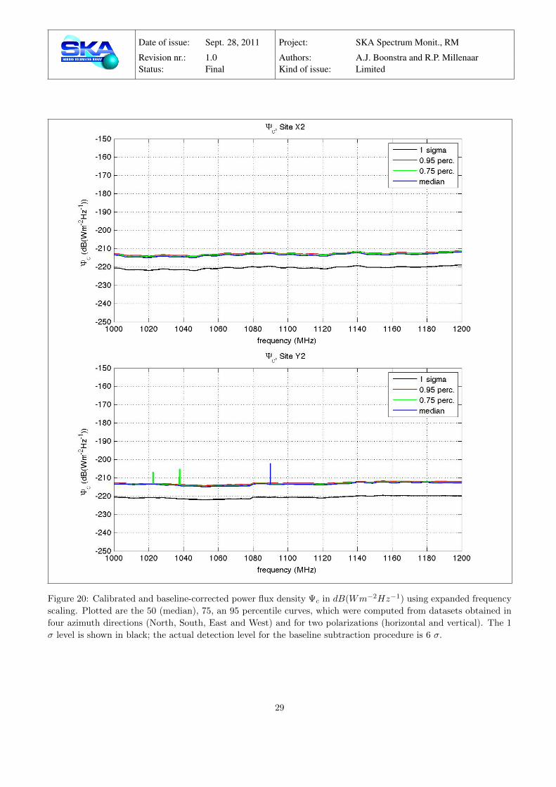
Figure 20: Calibrated and baseline-corrected power flux density Ψc in dB(Wm−2Hz−1) using expanded frequency
scaling. Plotted are the 50 (median), 75, an 95 percentile curves, which were computed from datasets obtained in
four azimuth directions (North, South, East and West) and for two polarizations (horizontal and vertical). The 1
σ level is shown in black; the actual detection level for the baseline subtraction procedure is 6 σ.
29
Page 30
Date of issue: Sept. 28, 2011 Project: SKA Spectrum Monit., RM
Revision nr.: 1.0 Authors: A.J. Boonstra and R.P. MillenaarStatus: Final Kind of issue: Limited
Figure 21: Calibrated and baseline-corrected power flux density Ψc in dB(Wm−2Hz−1) using expanded frequency
scaling. Plotted are the 50 (median), 75, an 95 percentile curves, which were computed from datasets obtained in
four azimuth directions (North, South, East and West) and for two polarizations (horizontal and vertical). The 1
σ level is shown in black; the actual detection level for the baseline subtraction procedure is 6 σ.
30
Page 31
Date of issue: Sept. 28, 2011 Project: SKA Spectrum Monit., RM
Revision nr.: 1.0 Authors: A.J. Boonstra and R.P. MillenaarStatus: Final Kind of issue: Limited
Figure 22: Calibrated and baseline-corrected power flux density Ψc in dB(Wm−2Hz−1) using expanded frequency
scaling. Plotted are the 50 (median), 75, an 95 percentile curves, which were computed from datasets obtained in
four azimuth directions (North, South, East and West) and for two polarizations (horizontal and vertical). The 1
σ level is shown in black; the actual detection level for the baseline subtraction procedure is 6 σ.
31
Page 32
Date of issue: Sept. 28, 2011 Project: SKA Spectrum Monit., RM
Revision nr.: 1.0 Authors: A.J. Boonstra and R.P. MillenaarStatus: Final Kind of issue: Limited
Figure 23: Calibrated and baseline-corrected power flux density Ψc in dB(Wm−2Hz−1) using expanded frequency
scaling. Plotted are the 50 (median), 75, an 95 percentile curves, which were computed from datasets obtained in
four azimuth directions (North, South, East and West) and for two polarizations (horizontal and vertical). The 1
σ level is shown in black; the actual detection level for the baseline subtraction procedure is 6 σ.
32
Page 33
Date of issue: Sept. 28, 2011 Project: SKA Spectrum Monit., RM
Revision nr.: 1.0 Authors: A.J. Boonstra and R.P. MillenaarStatus: Final Kind of issue: Limited
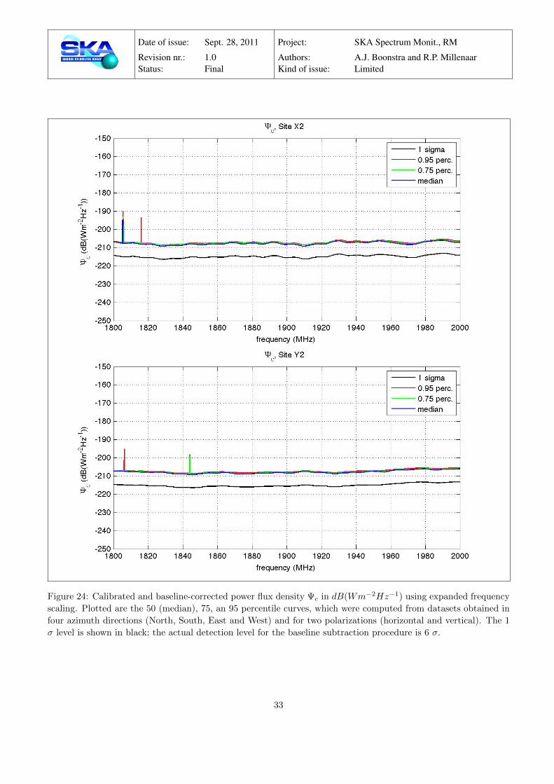
Figure 24: Calibrated and baseline-corrected power flux density Ψc in dB(Wm−2Hz−1) using expanded frequency
scaling. Plotted are the 50 (median), 75, an 95 percentile curves, which were computed from datasets obtained in
four azimuth directions (North, South, East and West) and for two polarizations (horizontal and vertical). The 1
σ level is shown in black; the actual detection level for the baseline subtraction procedure is 6 σ.
33
Page 34
Date of issue: Sept. 28, 2011 Project: SKA Spectrum Monit., RM
Revision nr.: 1.0 Authors: A.J. Boonstra and R.P. MillenaarStatus: Final Kind of issue: Limited
2.2.3 Spectral power flux density, sites X3 and Y3
34
Page 35
Date of issue: Sept. 28, 2011 Project: SKA Spectrum Monit., RM
Revision nr.: 1.0 Authors: A.J. Boonstra and R.P. MillenaarStatus: Final Kind of issue: Limited
Figure 25: Calibrated and baseline-corrected power flux density Ψc in dB(Wm−2Hz−1) using expanded frequency
scaling. Plotted are the 50 (median), 75, an 95 percentile curves, which were computed from datasets obtained in
four azimuth directions (North, South, East and West) and for two polarizations (horizontal and vertical). The 1
σ level is shown in black; the actual detection level for the baseline subtraction procedure is 6 σ.
35
Page 36
Date of issue: Sept. 28, 2011 Project: SKA Spectrum Monit., RM
Revision nr.: 1.0 Authors: A.J. Boonstra and R.P. MillenaarStatus: Final Kind of issue: Limited
Figure 26: Calibrated and baseline-corrected power flux density Ψc in dB(Wm−2Hz−1) using expanded frequency
scaling. Plotted are the 50 (median), 75, an 95 percentile curves, which were computed from datasets obtained in
four azimuth directions (North, South, East and West) and for two polarizations (horizontal and vertical). The 1
σ level is shown in black; the actual detection level for the baseline subtraction procedure is 6 σ.
36
Page 37
Date of issue: Sept. 28, 2011 Project: SKA Spectrum Monit., RM
Revision nr.: 1.0 Authors: A.J. Boonstra and R.P. MillenaarStatus: Final Kind of issue: Limited
Figure 27: Calibrated and baseline-corrected power flux density Ψc in dB(Wm−2Hz−1) using expanded frequency
scaling. Plotted are the 50 (median), 75, an 95 percentile curves, which were computed from datasets obtained in
four azimuth directions (North, South, East and West) and for two polarizations (horizontal and vertical). The 1
σ level is shown in black; the actual detection level for the baseline subtraction procedure is 6 σ.
37
Page 38
Date of issue: Sept. 28, 2011 Project: SKA Spectrum Monit., RM
Revision nr.: 1.0 Authors: A.J. Boonstra and R.P. MillenaarStatus: Final Kind of issue: Limited
Figure 28: Calibrated and baseline-corrected power flux density Ψc in dB(Wm−2Hz−1) using expanded frequency
scaling. Plotted are the 50 (median), 75, an 95 percentile curves, which were computed from datasets obtained in
four azimuth directions (North, South, East and West) and for two polarizations (horizontal and vertical). The 1
σ level is shown in black; the actual detection level for the baseline subtraction procedure is 6 σ.
38
Page 39
Date of issue: Sept. 28, 2011 Project: SKA Spectrum Monit., RM
Revision nr.: 1.0 Authors: A.J. Boonstra and R.P. MillenaarStatus: Final Kind of issue: Limited
Figure 29: Calibrated and baseline-corrected power flux density Ψc in dB(Wm−2Hz−1) using expanded frequency
scaling. Plotted are the 50 (median), 75, an 95 percentile curves, which were computed from datasets obtained in
four azimuth directions (North, South, East and West) and for two polarizations (horizontal and vertical). The 1
σ level is shown in black; the actual detection level for the baseline subtraction procedure is 6 σ.
39
Page 40
Date of issue: Sept. 28, 2011 Project: SKA Spectrum Monit., RM
Revision nr.: 1.0 Authors: A.J. Boonstra and R.P. MillenaarStatus: Final Kind of issue: Limited
Figure 30: Calibrated and baseline-corrected power flux density Ψc in dB(Wm−2Hz−1) using expanded frequency
scaling. Plotted are the 50 (median), 75, an 95 percentile curves, which were computed from datasets obtained in
four azimuth directions (North, South, East and West) and for two polarizations (horizontal and vertical). The 1
σ level is shown in black; the actual detection level for the baseline subtraction procedure is 6 σ.
40
Page 41
Date of issue: Sept. 28, 2011 Project: SKA Spectrum Monit., RM
Revision nr.: 1.0 Authors: A.J. Boonstra and R.P. MillenaarStatus: Final Kind of issue: Limited
Figure 31: Calibrated and baseline-corrected power flux density Ψc in dB(Wm−2Hz−1) using expanded frequency
scaling. Plotted are the 50 (median), 75, an 95 percentile curves, which were computed from datasets obtained in
four azimuth directions (North, South, East and West) and for two polarizations (horizontal and vertical). The 1
σ level is shown in black; the actual detection level for the baseline subtraction procedure is 6 σ.
41
Page 42
Date of issue: Sept. 28, 2011 Project: SKA Spectrum Monit., RM
Revision nr.: 1.0 Authors: A.J. Boonstra and R.P. MillenaarStatus: Final Kind of issue: Limited
Figure 32: Calibrated and baseline-corrected power flux density Ψc in dB(Wm−2Hz−1) using expanded frequency
scaling. Plotted are the 50 (median), 75, an 95 percentile curves, which were computed from datasets obtained in
four azimuth directions (North, South, East and West) and for two polarizations (horizontal and vertical). The 1
σ level is shown in black; the actual detection level for the baseline subtraction procedure is 6 σ.
42
Page 43
Date of issue: Sept. 28, 2011 Project: SKA Spectrum Monit., RM
Revision nr.: 1.0 Authors: A.J. Boonstra and R.P. MillenaarStatus: Final Kind of issue: Limited
Figure 33: Calibrated and baseline-corrected power flux density Ψc in dB(Wm−2Hz−1) using expanded frequency
scaling. Plotted are the 50 (median), 75, an 95 percentile curves, which were computed from datasets obtained in
four azimuth directions (North, South, East and West) and for two polarizations (horizontal and vertical). The 1
σ level is shown in black; the actual detection level for the baseline subtraction procedure is 6 σ.
43
Page 44
Date of issue: Sept. 28, 2011 Project: SKA Spectrum Monit., RM
Revision nr.: 1.0 Authors: A.J. Boonstra and R.P. MillenaarStatus: Final Kind of issue: Limited
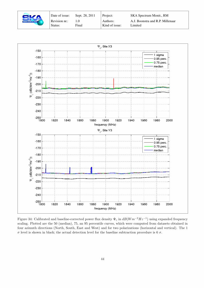
Figure 34: Calibrated and baseline-corrected power flux density Ψc in dB(Wm−2Hz−1) using expanded frequency
scaling. Plotted are the 50 (median), 75, an 95 percentile curves, which were computed from datasets obtained in
four azimuth directions (North, South, East and West) and for two polarizations (horizontal and vertical). The 1
σ level is shown in black; the actual detection level for the baseline subtraction procedure is 6 σ.
44
Page 45
Date of issue: Sept. 28, 2011 Project: SKA Spectrum Monit., RM
Revision nr.: 1.0 Authors: A.J. Boonstra and R.P. MillenaarStatus: Final Kind of issue: Limited
2.2.4 Spectral power flux density, sites X4 and Y4
45
Page 46
Date of issue: Sept. 28, 2011 Project: SKA Spectrum Monit., RM
Revision nr.: 1.0 Authors: A.J. Boonstra and R.P. MillenaarStatus: Final Kind of issue: Limited
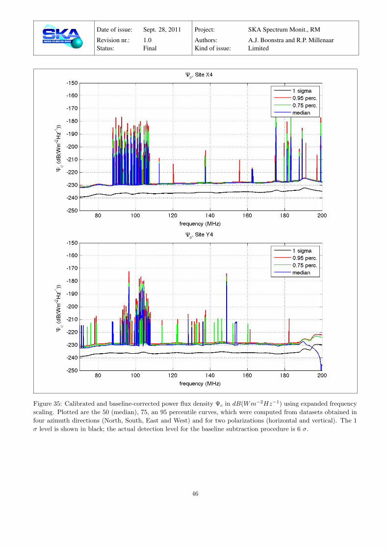
Figure 35: Calibrated and baseline-corrected power flux density Ψc in dB(Wm−2Hz−1) using expanded frequency
scaling. Plotted are the 50 (median), 75, an 95 percentile curves, which were computed from datasets obtained in
four azimuth directions (North, South, East and West) and for two polarizations (horizontal and vertical). The 1
σ level is shown in black; the actual detection level for the baseline subtraction procedure is 6 σ.
46
Page 47
Date of issue: Sept. 28, 2011 Project: SKA Spectrum Monit., RM
Revision nr.: 1.0 Authors: A.J. Boonstra and R.P. MillenaarStatus: Final Kind of issue: Limited
Figure 36: Calibrated and baseline-corrected power flux density Ψc in dB(Wm−2Hz−1) using expanded frequency
scaling. Plotted are the 50 (median), 75, an 95 percentile curves, which were computed from datasets obtained in
four azimuth directions (North, South, East and West) and for two polarizations (horizontal and vertical). The 1
σ level is shown in black; the actual detection level for the baseline subtraction procedure is 6 σ.
47
Page 48
Date of issue: Sept. 28, 2011 Project: SKA Spectrum Monit., RM
Revision nr.: 1.0 Authors: A.J. Boonstra and R.P. MillenaarStatus: Final Kind of issue: Limited
Figure 37: Calibrated and baseline-corrected power flux density Ψc in dB(Wm−2Hz−1) using expanded frequency
scaling. Plotted are the 50 (median), 75, an 95 percentile curves, which were computed from datasets obtained in
four azimuth directions (North, South, East and West) and for two polarizations (horizontal and vertical). The 1
σ level is shown in black; the actual detection level for the baseline subtraction procedure is 6 σ.
48
Page 49
Date of issue: Sept. 28, 2011 Project: SKA Spectrum Monit., RM
Revision nr.: 1.0 Authors: A.J. Boonstra and R.P. MillenaarStatus: Final Kind of issue: Limited
Figure 38: Calibrated and baseline-corrected power flux density Ψc in dB(Wm−2Hz−1) using expanded frequency
scaling. Plotted are the 50 (median), 75, an 95 percentile curves, which were computed from datasets obtained in
four azimuth directions (North, South, East and West) and for two polarizations (horizontal and vertical). The 1
σ level is shown in black; the actual detection level for the baseline subtraction procedure is 6 σ.
49
Page 50
Date of issue: Sept. 28, 2011 Project: SKA Spectrum Monit., RM
Revision nr.: 1.0 Authors: A.J. Boonstra and R.P. MillenaarStatus: Final Kind of issue: Limited
Figure 39: Calibrated and baseline-corrected power flux density Ψc in dB(Wm−2Hz−1) using expanded frequency
scaling. Plotted are the 50 (median), 75, an 95 percentile curves, which were computed from datasets obtained in
four azimuth directions (North, South, East and West) and for two polarizations (horizontal and vertical). The 1
σ level is shown in black; the actual detection level for the baseline subtraction procedure is 6 σ.
50
Page 51
Date of issue: Sept. 28, 2011 Project: SKA Spectrum Monit., RM
Revision nr.: 1.0 Authors: A.J. Boonstra and R.P. MillenaarStatus: Final Kind of issue: Limited
Figure 40: Calibrated and baseline-corrected power flux density Ψc in dB(Wm−2Hz−1) using expanded frequency
scaling. Plotted are the 50 (median), 75, an 95 percentile curves, which were computed from datasets obtained in
four azimuth directions (North, South, East and West) and for two polarizations (horizontal and vertical). The 1
σ level is shown in black; the actual detection level for the baseline subtraction procedure is 6 σ.
51
Page 52
Date of issue: Sept. 28, 2011 Project: SKA Spectrum Monit., RM
Revision nr.: 1.0 Authors: A.J. Boonstra and R.P. MillenaarStatus: Final Kind of issue: Limited
Figure 41: Calibrated and baseline-corrected power flux density Ψc in dB(Wm−2Hz−1) using expanded frequency
scaling. Plotted are the 50 (median), 75, an 95 percentile curves, which were computed from datasets obtained in
four azimuth directions (North, South, East and West) and for two polarizations (horizontal and vertical). The 1
σ level is shown in black; the actual detection level for the baseline subtraction procedure is 6 σ.
52
Page 53
Date of issue: Sept. 28, 2011 Project: SKA Spectrum Monit., RM
Revision nr.: 1.0 Authors: A.J. Boonstra and R.P. MillenaarStatus: Final Kind of issue: Limited
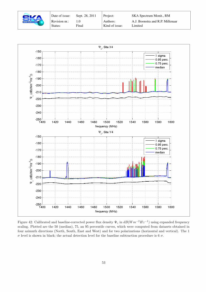
Figure 42: Calibrated and baseline-corrected power flux density Ψc in dB(Wm−2Hz−1) using expanded frequency
scaling. Plotted are the 50 (median), 75, an 95 percentile curves, which were computed from datasets obtained in
four azimuth directions (North, South, East and West) and for two polarizations (horizontal and vertical). The 1
σ level is shown in black; the actual detection level for the baseline subtraction procedure is 6 σ.
53
Page 54
Date of issue: Sept. 28, 2011 Project: SKA Spectrum Monit., RM
Revision nr.: 1.0 Authors: A.J. Boonstra and R.P. MillenaarStatus: Final Kind of issue: Limited
Figure 43: Calibrated and baseline-corrected power flux density Ψc in dB(Wm−2Hz−1) using expanded frequency
scaling. Plotted are the 50 (median), 75, an 95 percentile curves, which were computed from datasets obtained in
four azimuth directions (North, South, East and West) and for two polarizations (horizontal and vertical). The 1
σ level is shown in black; the actual detection level for the baseline subtraction procedure is 6 σ.
54
Page 55
Date of issue: Sept. 28, 2011 Project: SKA Spectrum Monit., RM
Revision nr.: 1.0 Authors: A.J. Boonstra and R.P. MillenaarStatus: Final Kind of issue: Limited
Figure 44: Calibrated and baseline-corrected power flux density Ψc in dB(Wm−2Hz−1) using expanded frequency
scaling. Plotted are the 50 (median), 75, an 95 percentile curves, which were computed from datasets obtained in
four azimuth directions (North, South, East and West) and for two polarizations (horizontal and vertical). The 1
σ level is shown in black; the actual detection level for the baseline subtraction procedure is 6 σ.
55
Page 56
Date of issue: Sept. 28, 2011 Project: SKA Spectrum Monit., RM
Revision nr.: 1.0 Authors: A.J. Boonstra and R.P. MillenaarStatus: Final Kind of issue: Limited
2.3 Sensitivity
56
Page 57
Date of issue: Sept. 28, 2011 Project: SKA Spectrum Monit., RM
Revision nr.: 1.0 Authors: A.J. Boonstra and R.P. MillenaarStatus: Final Kind of issue: Limited
Figure 45: Sensitivity ∆Ψ in dB(Wm−2Hz−1) estimates based on calibrated Trec curves. Plotted are the median
curves computed using data obtained in four azimuth directions (North, South, East, West) and two polarizations
(horizontal and vertical). The depicted estimations are 6σ values, but as these curves are based on Trec (and not
on Tsys) the underestimation factor is at least 3 dB. Please note the mid-band spikes, which are instrumental
artefacts.
57
Page 58
Date of issue: Sept. 28, 2011 Project: SKA Spectrum Monit., RM
Revision nr.: 1.0 Authors: A.J. Boonstra and R.P. MillenaarStatus: Final Kind of issue: Limited
Appendix A. Calibration results
58
Page 59
Date of issue: Sept. 28, 2011 Project: SKA Spectrum Monit., RM
Revision nr.: 1.0 Authors: A.J. Boonstra and R.P. MillenaarStatus: Final Kind of issue: Limited
A1. Gain
Figure 46: Calibrated gain curves G in dB: shown are the median values for each of the sites, computed using data
obtained in four azimuth directions (North, South, East, West) and two polarizations (horizontal and vertical).
Only the in-band sections are depicted; the “jumps” are band transitions.
59
Page 60
Date of issue: Sept. 28, 2011 Project: SKA Spectrum Monit., RM
Revision nr.: 1.0 Authors: A.J. Boonstra and R.P. MillenaarStatus: Final Kind of issue: Limited
A2. Receiver and system temperature
Figure 47: Receiver temperature Trec in K: shown are the median values for each of the sites, computed using data
obtained in four azimuth directions (North, South, East, West) and two polarizations (horizontal and vertical).
60
Page 61
Date of issue: Sept. 28, 2011 Project: SKA Spectrum Monit., RM
Revision nr.: 1.0 Authors: A.J. Boonstra and R.P. MillenaarStatus: Final Kind of issue: Limited
Figure 48: System temperature Tsys in K: shown are the median values for each of the sites, computed using data
obtained in four azimuth directions (North, South, East, West) and two polarizations (horizontal and vertical).
61
Page 62
Date of issue: Sept. 28, 2011 Project: SKA Spectrum Monit., RM
Revision nr.: 1.0 Authors: A.J. Boonstra and R.P. MillenaarStatus: Final Kind of issue: Limited
A3. Calibrated spectra, all sites
Figure 49: Calibrated but not baseline-corrected power flux density Ψ in dB(Wm−2Hz−1). Depicted are the 75
percentile curves, which were computed from datasets obtained in four azimuth directions (North, South, East and
West) and for two polarizations (horizontal and vertical).
62
Page 63
Date of issue: Sept. 28, 2011 Project: SKA Spectrum Monit., RM
Revision nr.: 1.0 Authors: A.J. Boonstra and R.P. MillenaarStatus: Final Kind of issue: Limited
A4. Calibrated spectra, percentiles
Figure 50: Calibrated but not baseline-corrected power flux density Ψ in dB(Wm−2Hz−1). Depicted are the 50
(median), 75, and 95 percentile curves, which were computed from datasets obtained in four azimuth directions
(North, South, East and West) and for two polarizations (horizontal and vertical).
63
Page 64
Date of issue: Sept. 28, 2011 Project: SKA Spectrum Monit., RM
Revision nr.: 1.0 Authors: A.J. Boonstra and R.P. MillenaarStatus: Final Kind of issue: Limited
Figure 51: Calibrated but not baseline-corrected power flux density Ψ in dB(Wm−2Hz−1). Depicted are the 50
(median), 75, and 95 percentile curves, which were computed from datasets obtained in four azimuth directions
(North, South, East and West) and for two polarizations (horizontal and vertical).
64
Page 65
Date of issue: Sept. 28, 2011 Project: SKA Spectrum Monit., RM
Revision nr.: 1.0 Authors: A.J. Boonstra and R.P. MillenaarStatus: Final Kind of issue: Limited
Figure 52: Calibrated but not baseline-corrected power flux density Ψ in dB(Wm−2Hz−1). Depicted are the 50
(median), 75, and 95 percentile curves, which were computed from datasets obtained in four azimuth directions
(North, South, East and West) and for two polarizations (horizontal and vertical).
65
Page 66
Date of issue: Sept. 28, 2011 Project: SKA Spectrum Monit., RM
Revision nr.: 1.0 Authors: A.J. Boonstra and R.P. MillenaarStatus: Final Kind of issue: Limited
Figure 53: Calibrated but not baseline-corrected power flux density Ψ in dB(Wm−2Hz−1). Depicted are the 50
(median), 75, and 95 percentile curves, which were computed from datasets obtained in four azimuth directions
(North, South, East and West) and for two polarizations (horizontal and vertical).
66