IZA DP No. 1542

Skills, Workforce Characteristics and Firm-LevelProductivity: Evidence from the MatchedABI/Employer Skills Survey

Fernando Galindo-RuedaJonathan Haskel

DI

SC

US

SI

ON

P

AP

ER

S

ER

IE

S

Forschungsinstitut

zur Zukunft der Arbeit

Institute for the Study

of Labor

March 2005

Skills, Workforce Characteristics

and Firm-Level Productivity: Evidence from the Matched ABI/Employer Skills Survey

Fernando Galindo-Rueda

CEP, London School of Economics, CeRiBA and IZA Bonn

Jonathan Haskel

Queen Mary, University of London, AIM, CeRiBA, CEPR and IZA Bonn

Discussion Paper No. 1542 March 2005

IZA

P.O. Box 7240 53072 Bonn

Germany

Phone: +49-228-3894-0 Fax: +49-228-3894-180

Email: iza@iza.org

Any opinions expressed here are those of the author(s) and not those of the institute. Research disseminated by IZA may include views on policy, but the institute itself takes no institutional policy positions. The Institute for the Study of Labor (IZA) in Bonn is a local and virtual international research center and a place of communication between science, politics and business. IZA is an independent nonprofit company supported by Deutsche Post World Net. The center is associated with the University of Bonn and offers a stimulating research environment through its research networks, research support, and visitors and doctoral programs. IZA engages in (i) original and internationally competitive research in all fields of labor economics, (ii) development of policy concepts, and (iii) dissemination of research results and concepts to the interested public. IZA Discussion Papers often represent preliminary work and are circulated to encourage discussion. Citation of such a paper should account for its provisional character. A revised version may be available directly from the author.

IZA Discussion Paper No. 1542 March 2005

ABSTRACT

Skills, Workforce Characteristics and Firm-Level Productivity: Evidence from the Matched ABI/Employer Skills Survey∗

We construct firm-level data set with matched productivity and qualification data by linking the Annual Business Inquiry and Employer Skills Survey for England. We first examine the effect of workplace skills and other characteristics such as part-time status and gender on both productivity and wages in English firms. We also investigate how productivity-implied returns to worker characteristics compare with wage-implied returns, therefore providing information on how rents are distributed between employers and employees. We find that firms with a higher share of college-educated, full-time and male workers also tend to be more productive, with considerable variations across sectors. The only robust difference in implied returns follows from part-timers, who tend to work for firms that pay too low wages for the observed productivity differences. Second, we study the effect of local skills on productivity controlling for skills at the firm. We find a positive and robust association, which is consistent with positive human capital externalities. JEL Classification: J2, J3, J7 Keywords: productivity, wages, skills, workforce characteristics, spillovers Corresponding author: Fernando Galindo-Rueda Centre for Economic Performance London School of Economics Houghton Street WC2A 2AE London United Kingdom Email: f.galindo-rueda@lse.ac.uk

∗ Financial support for this research comes from the DfES, the DTI and the ESRC/EPSRC Advanced Institute of Management Research, grant number RES-331-25-0030 with the work undertaken at the Centre for Research into Business Activity, CeRiBA at the Business Data Linking Branch at the ONS; we are grateful to all institutions concerned for their support. We thank the project’s steering board for helpful comments on an earlier draft. In this paper we use the ONS ARD data set, which is a research tool and may not entirely match official published figures. ESS data have been provided by the Department for Education and Skills. Census and ARD output is Crown copyright and is reproduced with the permission of the Controller of HMSO and the Queen's Printer for Scotland. The use of the ONS statistical data in this work does not imply the endorsement of the ONS or any other UK government department in relation to the interpretation or analysis of the statistical data. The usual disclaimer applies.

Executive summary

Considerable policy effort has been devoted to improving the skills and qualification

attainment levels in the UK population. What are the economic payoffs to this policy?

There might be at least three: increased wages of workers, increased productivity of firms

where they work and increased productivity of other firms and workers, say in the same

area, from a higher pool of skilled workers to interact with. Thus this paper seeks to

address three questions:

1. What is the effect of skills on firm productivity?

2. What are the effects of skills on wages and how do they compare with the effect

on firms’ productivity?

3. Is there any evidence of externalities to skill acquisition in the form of increased

productivity for firms from skills outside the firm in the local region, controlling

for skills within the firm?

Existing evidence on these issues is surprisingly patchy. Regarding the first question,

whilst there are number of UK studies of firm-level productivity almost none of them have

data on skills at the firm. Equally, studies of skill surveys typically do not have data that

enable to construct measures of the productivity of the firm where workers work. Thus

evidence of the effect of skills on firm productivity is very thin.

Such evidence as we do possess is therefore rather indirect and consists of studies of the

effect of skills on wages. Under the hypothesis that wages reflect productivity the approach

behind these studies is sufficient to establish both the effect of skills on workers wages and

on firm productivity. A number of these studies have uncovered, for example, that the

effect of level 1 and 2 vocational qualifications on wages is more or less zero, suggesting

that the effect on productivity is therefore zero as well. However, it would be desirable to

test this hypothesis further. Another important question that these studies have not been

able to address so far is whether firms reward characteristics of their workforce as implied

by wages to a similar extent as implied by observed productivity differences.

Regarding the third question, the issue here is whether firms, controlling for their internal

skills, get a productivity boost when in an area with more skilled workers. Alfred Marshall

2

suggested that proximity to skilled workers allows for better interactions, swapping

information etc. in ways that might raise productivity for other firms and workers. This is

an important policy issue for if there are positive spillovers or externalities from skill

acquisition to other firms then there might be an undersupply of training, under the

hypothesis that firms, quite reasonably, do not consider the benefits to other firms when

making their own decisions about how much training to offer. Indeed, a similar reasoning

may apply to individuals when they decide whether to invest into attaining further

qualifications. Thus the economy might be underinvesting in human capital which might

justify intervention through a series of policy levers such as taxes, subsidies and the like.

This is again a question on which evidence is remarkably thin. Since there has been

considerable difficulty in assembling data on skills and productivity internal to the firm

level this has also precluded studying the effect of skills external to the firm (since any such

effect would suffer from the omission of internal skills which are likely correlated with

external skills).

Thus our main contributions in this paper are to assemble the data necessary to examine

these questions and to provide insights on these questions. To do this we first merged data

on firm level productivity from the Annual Business Inquiry, with data from a large survey

of English establishments known as the Employer Skills Survey, which provides

information on workforce skills.

To investigate the role of outside skills, we added external skills measures from the

population Census to measure local skill levels. This gives us very detailed measures of

skills in a very localized market. Thus we can examine the association between local skills

and firm productivity controlling for firm-level skills and other local area characteristics.

Second, previous work has focused on manufacturing. This work deals with both for

services and manufacturing. The latter is potentially important since the service sector

comprises such a large and ever growing section of the economy.

Our method then is to examine productivity and wage regressions for the same firm. We

start by examining the impact of internal skills. Specifically, we regress productivity on

skills and wages on skills, conditioning on other inputs. We examine the coefficients on

skills in both equations. The hypothesis that the productivity impact of skills is reflected in

3

wages implies that the marginal effects from skills in both equations should be the same and

thus this can be tested. Any differences in coefficients would indicate, that, for example,

workers of a certain skill type have an effect on productivity of x but are being paid more or

less then x in return, suggesting that the rents from skills are accruing either to the employer

(if workers are paid less) or the employee (if workers are paid more). (Note however that

such rents might the accrue to other factors: so for example if employers profit from hiring

skilled workers in a certain locality they might keep such profits if there is no entry, or land

prices would be bid up until profits were exhausted). Of course, the standard criticism is

that both wage and productivity equations suffer from a host of omitted variables that

cannot be measured. However, in this case we are comparing coefficients from estimating

the equations together and any biases from omission, which would affect a coefficient in a

single regression, should not affect the relative coefficients.

We turn to the impact of external skills by then taking the production functions set out

above and adding the external skill measures.

Regarding the three questions we started with our data suggests:

1. Overall, increased skills raise company productivity. However, this overall

picture hides important variation within different skill types. In particular,

higher-level qualifications at the firm have a much more robust positive effect on

productivity then lower level skills.

2. Regarding the comparison of skills and wages, there is a never a statistically

significant difference in manufacturing (although it is positive, suggesting that

skill rents accrue to workers). Services however show a statistically negative

significant difference for level 3 and level 4 skills, suggesting that the rents are

accruing to employees in service firms with more educated workers. We also

examine the comparison of returns for gender and part-timers. For gender there

is never a statistically significant difference but firms with more part-timers

appear to systematically underpay their workers relative to their productivity,

suggesting that rents go to firms in the case of part-timers.

3. Finally, we do find some evidence for skills externalities as seen from higher

productivity levels in comparable firms, also regarding their own stock of

internal skills.

4

1. Introduction

There is considerable interest amongst economists and policy makers as to which type of

workplace characteristics are more conducive to higher levels of productivity. Investment

in human capital through higher qualifications and training is considered as a key step

towards achieving sustained long-term productivity and prosperity gains in an economy.

Despite the fact that these investments are observed to provide a direct economic return to

the individuals who benefit from them, there is little direct evidence about possible wider

returns. Wider returns might arise in two particular ways. First, internally, workers seem to

gain from skill acquisition but firms might also gain to an equal or greater or lesser extent.

Second, externally, it has been suggested that firms gain from skills in a local area due to

interactions and related spillovers and hence other firms might also gain from the skill level

of a given firm or the surrounding population in general. Possible externalities might create

differences between individual and social returns which form a key part of the rationale for

public intervention in promoting human capital. This paper aims to shed light on this

subject by addressing three simple questions.

First, is it true that firms with a more educated workforce also tend to be more productive?

Second, how does the association between productivity and workforce characteristics, such

as qualifications or gender, from productivity equations compare with the association

between wages and workforce characteristics from wage equations? Third, is there any

evidence of externalities to investment in human capital through qualifications in the form

of increased productivity for firms that are located in areas with a better access to a more

educated population, controlling for skills within the firm and other area-level

characteristics?

Our method is as follows. To compare the characteristics/wages association with the

characteristics/productivity association we need data on the wages, characteristics and

productivity of workers and firms. Typical (individual level) wage data set have

information on wages and characteristics but not on the productivity of the firm where the

individuals work. Typical (firm-level level) productivity data sets have data on productivity

and wages but not on educational and other characteristics of the workers. Thus we build a

5

firm-level data set by matching firm-level productivity data, drawn from the UK business

census, with firm-level worker education data, drawn from a special survey for England

undertaken by the UK Department for Education.

Our results are novel for the UK but we believe also for the wider related literature.1

Regarding the internal effects of skills and other worker characteristics, we investigate not

only higher education, but also how low and middle level qualifications correlate with

business productivity. Here we find a mostly positive effect on productivity of higher

qualifications, but little robust effect from lower level qualifications. We do not restrict our

analysis to manufacturing firms as done in similar US studies such as Hellerstein et al

(1999) and Hellerstein and Neumark (2003) but consider services too. We find that

consistently across sectors, that whilst productivity of firms with higher shares of part

timers is lower, wages are lower still. However, we also find that higher skilled workers or

females are rewarded in line with productivity differences

Regarding the subject of skill spillovers, we do observe in our data some support for the

hypothesis of positive human capital externalities, based on the evidence that firms located

in more educated areas (either in terms of residents or workers) also tend to be more

productive. This finding applies to both manufacturing and services and confirms earlier

US estimates restricted to manufacturing by Moretti (2002 and forthcoming).

Two particular problems with our work will become apparent in what follows. First, by

virtue of the data provided we have rather small samples at times which leads to often

imprecise estimates. Second, we do not have pseudo-experimental data to establish

causality between workplace characteristics and productivity but this is unlikely to affect

the productivity-wage comparisons which are useful in that they show to which extent

wages reflect observed productivity differentials, and implicitly tell us about how economic

rents are split between workers and other factors of production.

This work is structured as follows. Section 2 explains the data linking process required to

build our matched dataset. Section 3 presents the data while Section 4 covers the basic

1 Our research draws on previous research by Haskel et al (2003) based on matched ESS and ABI manufacturing firms.

6

econometric framework. Drawing on this, Section 5 presents and discusses the estimation

results and Section 6 concludes.

2. Skills measures from the ESS, Census and data matching

The Annual Business Inquiry (ABI)

The ABI is an annual business survey that covers almost all production and construction

activities as well as distribution and other service activities2 (see Criscuolo et al, 2003, for

an extensive description). Information on the universe of UK businesses is maintained by

the Office of National Statistics using the Inter-Department Business Register (IDBR).

Although the ABI is colloquially referred to as a census, it is in fact a stratified sample

drawn from the IDBR. It has full coverage for all businesses with 250 employees or more,

and becomes sample of smaller businesses according to stratification rules based on size,

region and industrial sector. The ABI reports information on output, employment, materials,

investment, wage costs, region, industry and business structure (presence of other plants in

the firm) and occasional questions such as R&D, e-commerce and computer expenditure.

We use data returned by businesses to the ONS from this inquiry.3

To reduce compliance costs, multi-plant businesses have some degree of choice in the way

they report the information to the ABI. They can report on all the plants individually or on

one or various groups of establishments/plants (the latter are called local units (LUs) in the

IDBR). Data is therefore collected at what is known as reporting unit (RU) level, where a

reporting unit can be a plant or a group of plants. Each reporting unit has its own unique RU

identification number, an enterprise and enterprise group identification number and the

identification numbers of the local units it is reporting on if applicable. Note therefore that 2 It does not cover some sectors, notably, the public administration and defence, agriculture, fishing, financial intermediation, non-private education, private households with employed persons and only has limited coverage on health and social work. 3 It is compulsory to return data if sampled. In theory we could potentially expand our data by including the firms who do not return data because they are not sampled, which are essentially small firms, but using data from the IDBR. The problem is that although the IDBR records the businesses’ region, industry, business structure, turnover and employment, turnover and employment are in many cases interpolated or severely out

7

RU data might refer to one or more plants. Only in the case of single-LU RUs there will be

no ambiguity with regards to the specific location of an RU. Furthermore, an enterprise

/firm might report the information requested by ONS through one or more reporting units.

We will refer to the former as multi-RU enterprises.

The Employers Skill Survey(ESS)

The ESS is a workplace level survey, which was first undertaken in 1999 and has been

repeated annually since 2001. It originally targeted a sample of 27,000 English

establishments, which was reduced to 4,000 establishments in 2002. The 2001 ESS sample

covered all sectors of the economy for plants with one or more employees. The survey

covers a range of subjects including recruitment problems, skills and proficiency and

training. For the purpose of this study we shall focus exclusively on the workforce skill

questions from the ESS.4

The basic skill information from the ESS is drawn as follows. First, firms are asked to

report the fraction of workers who are in each of nine specified occupational groups. The

occupations are managers, professions, associates, administrators, skilled manual, personal,

sales, machine operatives and elementary occupations. Second, firms are asked to specify

the most common qualification held by their employees in each of these nine occupational

groups. The qualifications they are asked to use are set out in the Appendix. Our firm level

skill measure thus simply uses the proportions of workers in each firm with each

qualification level, which we combined into levels 4/5, 3, 2, 1 and other or none.5 This

standard classification of qualifications combines academic and vocational qualifications

grouped together.6

of date or both, and therefore cannot be used for reliable productivity analysis (see Criscuolo, Haskel and Martin, 2003, for details: in 2000, 80% of firms under 20 had never returned an employment questionnaire). 4 For more information on the ESS see IFF Research Ltd (2002). 5 Our analysis of spillovers has focused so far on the NVQ-equivalent shares as controls for firm level skills. In their analysis of the effects of firm level skills on productivity, Haskel, Hawkes and Pereira (2003) used a wide number of measures and alternative specifications producing similar results. Our preferred choice is to stick to the standard British classification as the firm-level measure of human capital, largely for consistency with our spillover human capital measure that will be described below. 6 For example, level 4/5 refers to higher education graduates and highest vocational qualifications. Level 3 basically corresponds to A-level equivalents whereas level 2 indicates individuals whose highest level of attainment is an O-level or GCSE equivalent which allows for satisfactory progress at the end of compulsory schooling into A-level type qualifications. Finally, level 1 captures lower levels of attainment at the end of

8

Matching the ABI and the ESS

The ESS 2001 consisted of a pilot in October 2000 and was in the field from November

2000 to April 2001. As the ABI is conducted mainly by financial year we match the ESS

2001 to the ABI 2000. Details of some of the issues surrounding the matching of both

datasets can be found in Hawkes (2003).

The matching of ESS LUs to ABI financial data proceeded as follows. We started with

27,032 surveyed LUs on the ESS, drawn by the DfES-commissioned contractor from the

BT business Directory. The only practical way to match these observations to available

productivity data from the ABI is through the Interdepartmental Business Register (IDBR),

from which the ABI is drawn. Although ONS provided a link of these ESS records to the

IDBR, this match was not hundred-percent successful because of differences in coverage

and, quite possibly, because of differences in the way in which establishments are recorded

in the IDBR and the BT Business Directory.7 The matching carried out by ONS used

statistical matching software linking the name of the business, address and postcode. ONS

provided us with a list of reliable matches, which accounted for 63 percent of the original

ESS sample (17,111 out of 27,032 ESS observations). Note however that the list provided

to us was neither a list of corresponding ABI reporting units (RU) or local units (LU) per se,

but the enterprise code (entref) available in the ABI and the identifying code variable

(iuniq) for the ESS sample.

As explained, an IDBR enterprise denoted by a particular entref code may contain more

than one RU and an RU can encompass more than a single LU. Unfortunately, ABI LUs do

not have reliable (i.e. non-imputed) input and output data unless they correspond to single-

plant RUs. Thus, for the purposes of linking both datasets, our primary target was to set up

matches of ESS LUs and ABI RUs. We will later return to discuss the feasibility and

appropriateness of conducting estimation at one level or another.

compulsory schooling for individuals who attain some sort of qualification. This would also include the most basic type of vocational attainment. 7 It is indeed possible that ESS establishments cover one or more than a single IDBR local units, as several companies have local units in the same or adjacent postcodes. Furthermore, not all enterprises in the IDBR have a probed or suitably updated internal structure. Information provided through the ESS need not necessarily correspond with any of the three levels of classification of information in the IDBR, namely enterprise, reporting and local unit, except for the case of single plant reporting units.

9

Because of the indeterminacy induced by having access to enterprise codes rather than RU

codes, we proceeded in two steps. Firstly, enterprises with a single RU were

straightforward to match through the enterprise code. This step matched 3,290 ESS

establishments to ABI RUs selected in 2000. The biggest loss of data is down to the fact

that many ESS establishments are only infrequently selected into the ABI from the IDBR

and therefore do not appear on the ABI returned sample in 2000. We cannot use these data

therefore. Some however corresponded to enterprises with multiple RUs. Thus to try to

obtain more valid matches, in the second step we dealt with these ambiguous cases. The

problem is essentially one of, for enterprises with more than one RU, knowing how to

identify which of the reporting units should be linked to the ESS LU that has been linked to

that particular enterprise. We decided to do this using postcode information from the ESS

and the LUs in each RU corresponding to multi-RU enterprises. We thus took all LUs

which are part of multi-RU enterprises and identified their “entref” code and their full

postcode. This gave 70,560 LUs. Some of these LUs however are in enterprises where

different RUs share the same full postcode; we dropped these, as it would be virtually

impossible to identify the “right” RU for the particular postcode an individual ESS

establishment. This leaves us with 62,701 ABI LUs from multi-RU enterprises. With no

loss of generality, we compressed this dataset so that there is a single record for every

existing combination of postcode and enterprise code. Linking the resulting set of multi-

plant LUs to the unmatched ESS establishments by entref code and full postcode gives us

799 extra establishments matched, approximately an improvement of 25 percent with

respect the original matches based on single RU enterprises.

Appending these 799 establishments to the dataset with matched ESS establishments to

single-RU enterprises we obtain a feasible sample of 4089 observations. In this dataset,

there are only 2847 unique RUs because the ESS has gathered information in several cases

from different establishments that belong to the same RU.

To summarise the process so far, it is helpful to note that 50059 selected RUs in the 2000

ABI have found no counterpart in the ESS, whereas 22942 ESS establishments were not

linked to a selected 2000 ABI RU. This means we can proceed to a further stage with

approximately a 15 percent of the original ESS sample.

10

From the sample of 4089 matched establishments, we have removed those with missing

data on turnover and employment, capital, female and part-time shares and value added.

This leaves 3,199 records. A summary of this matching process and the industrial

breakdown of the matched dataset are set out in Table 1.

Linking the ESS to the Census of Population area-data

We also compute a measure of human capital density in geographic areas using the Census

of Population, 2001 with qualifications data at the local authority level. In England and

Wales, shares by areas for the available variable denoting highest level of qualification are

derived from responses to both the academic and vocational qualification questions.

In order to match Census data to the new ABI-ESS data set, we use as geographical link

identifier the postcode of the ESS establishment successfully linked to an ABI reporting

unit. This implies that both internal and external qualification data apply to the same notion

of business establishment and hence estimates should in principle not be affected by

measurement error differences.8

3. Descriptive statistics

Table 2 shows simple descriptive statistics by manufacturing (814 observations) and

services (2,229).9 Our descriptive statistics and estimates are not weighted because we

cannot meaningfully calculate the exact theoretical sampling weights for the matched

dataset. As a result, all our statements will therefore refer to our matched sample. The

main focus of our paper, namely the estimated coefficients, will not be affected as long as

the true coefficients are homogeneous within the estimation subsamples.10 The first few

rows in Table 2 display the average across firms in each sector for the share of employees

qualified at different levels. The service sector firms employ on average a higher proportion

8 For example, if internal skills are measured with more error than surrounding skills, the coefficient on the former will tend to underestimate the true effect whereas the opposite will hold for the latter. 9 The remaining observations correspond to the construction sector, which is included only in full-sample estimates displayed below but not in the split-sector estimates. 10 Weighting using wrong weights may lead to potentially higher error.

11

of more educated workers, employing higher fractions of workers with levels 4, 3 and 2.

This sector also displays a higher dispersion, which is partly explained by significant

sectoral differences within services.

Firms in the service sector sample also tend to have more employees and a more unequal

size distribution. Note however that female and part-time forms of employment are much

more prevalent in service sector firms.11 The average manufacturing firm has only one

quarter of female employees compared with one in services, with slightly more than one

half. Part time labour is rather infrequent in manufacturing, with the average firm at six

percent, very distant from services’ average of above one third.

Interestingly, manufacturing firms tend to have higher wages per employee, labour

productivity and capital and intermediate goods intensity relative to the number of

employees. This confirms the perception of services as a more labour intensive sector.

Foreign ownership is more frequent in manufacturing. Also, a bigger proportion of

establishments in services are part of multi-plant reporting units (79 percent) compared with

manufacturing (57 percent), implying that possible measurement error from matching of

single LUs to RUs is likely to higher in the service sector.

We provide further details on the distribution of firm-level skills within sectors in Figure 1.

It shows the distribution of establishment’s qualification intensity (as proxied by the share

with level 3 or higher) for different sectors. Trade, hospitality and transport show the

biggest incidence of establishments without a qualified workforce. Manufacturing has the

most even distribution whereas all other groups display big mass points at the lowest and

highest extremes. As one would expect, business services and education and health display

the biggest mass of firms with high skills.

This bimodal shape with firms either employing many low skilled or many high skilled, but

relatively few employing those in the middle has not, we believe, been directly documented

at the firm level, and seems particularly evident in services. Thus as manufacturing declines

11 These numbers are unweighted. To obtain numbers that are representative of the UK economy distribution of firms we would have to weight accounting for the stratification in the ABI, the sampling of ESS establishments and the possible non-random matching of ABI and ESS observations. A further adjustment for employment in firms would be required to reflect the characteristics of the population of employees, rather than firms.

12

the economy seems likely to become more polarised between firms employing high and low

shares of skilled/educated workers. Manning and Goos (2004) have remarked on this

indirectly via recent growth of both highly skilled and low skilled jobs relative to “middle-

rank” jobs (using the New Earnings Survey), see also Acemoglu (2004) for the US.

Table 3 sets out the data in a slightly different way. It starts by ranking all the matched ESS

establishments by their share of workers with level 3 or above and splitting them into

quintiles. Thus looking at row 1, the lowest quartile has, on average, 0.5% of its workforce

qualified up to level 3 or higher and the highest quartile, row 5, has 97.7% so qualified.

Row 2 shows the corresponding data for the shares up to level 4 and above. Rows 3 and 4

show that average labour productivity (log unit gross value added) and average unit labour

costs rise monotonically with skill intensity, whilst the other rows suggest somewhat higher

capital intensity but not so much higher intensity of intermediate goods. Share of females is

highest at the extremes of the skill distribution and about the same value, but part-timers

feature much more in low skill establishments. Finally, firms with higher fractions

qualified are also located in areas (local authority districts) with higher fractions of more

qualified residents and workers, according to 2001 Census data.

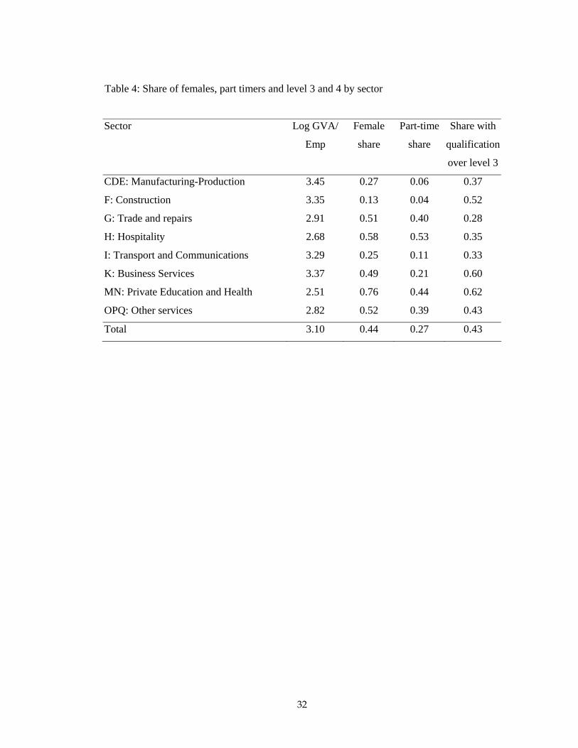
We conclude our summary description of the data with Table 4, which shows the average

labour productivity, shares of females, part-timers and level 3 and 4 qualifications of firms

by sector. Not surprisingly, women are concentrated in education and hospitality whereas

male-populated firms are predominant in construction, transport and manufacturing. There

are few part-timers in manufacturing, but many in hospitality and education. Manufacturing

is relatively skill intensive, and skills are substantially concentrated in education and

business services.

4. Estimation approach

Suppose the production function for firm i can be specified in a general Cobb-Douglas form

1

( ) jn

i i jj

Y A QX γ

=

= ∏ , (1)

13

where QXj denotes the quality of input Xj, where there are j=1…n inputs and A is an

idiosyncratic productivity term. For simplicity of notation we omit the subindex i to

indicate variation across firms. Let us suppose further we can write QXn of the n’th input,

labour, as consisting of m+1 sub-inputs indexed by k=0,1,…m:

∑=

+=m

kkkn LQX

0)1( φ (2)

where 1+φk indicates of the relative productivity of labour input type k relative to that of the

base type k=0 (and so φ is the proportional difference in quality, with a simple

normalisation of φ0=0). Implicit in (2) is that different types of labour are infinitely

substitutable. This may be a reasonable approximation when considering small changes in

the composition of a firm’s workforce.12 Equation (2) has the convenient property that the

relative marginal productivity of type k to type 0, (∂Y/∂Lk)/(∂Y/∂L0)=(1+φk), is constant,

implying that marginal productivity does not depend on employment levels of either type.

Assuming there are three basic inputs in the production of output, namely capital,

intermediate goods and labour, substitution of (2) into (1) gives the extended production

function

1

ln ln ln ln ln 1m

ki i M i K i L i k

k i

LY A M K LL

γ γ γ φ=

⎡ ⎤⎛ ⎞⎛ ⎞= + + + +⎢ ⎥⎜ ⎟⎜ ⎟⎝ ⎠⎝ ⎠⎣ ⎦

∑ . (3)

Let us suppose that different labour types only differ in terms of qualification attainment. If

relative wages equal relative marginal products then log(wk/w0)=log((1+φk)≈ φk. Thus a

possible test of competitiveness in the labour market for skills would imply a comparison of

the returns implied by equation (3) with the observed returns in standard Mincer-type

earnings regressions at the individual level. Since we have information on total wage costs

(W) at the firm level for the same firms on which we can conduct the productivity analysis,

a more balanced assessment could be achieved by exploring how skill intensity relates to

average firm-level wages. Log unit wage (W/L) in a firm can be decomposed into a

14

weighted sum of unit wages by skills in the firm. Under the stated assumptions, relative

wages are constant and a log approximation allows us to write the firm-level counterpart of

the standard Mincer regression

∑∑==

+≅⋅=m

kikk

m

kiokiikii LLwwLLLW

10, )/('ln))/(ln()/ln( φ , (4)

where the firm level specific baseline can vary as a result of idiosyncratic differences.

Note that aggregating to the level of the firm implies that estimates will tell us about the

overall relationship between skills intensity and average wages. A positive relationship,

however, may mask different mechanisms if we relax some of the assumptions underlying

this aggregation. Essentially, higher skills may be associated with higher wages but, to give

an example, a highly unionised workplace may imply considerable wage compression,

leading to high average wages in skilled firms but more educated workers being paid only

marginally more than their less educated counterparts.13

The above example divided labour into types according to a single characteristic. In our

data we have a number of labour characteristics: fractions with different qualification levels,

part-timers and female. Thus we put the k types of workers into 6 categories, 4 skill groups,

part-timers and female; all entering additively in the quality of labour term and assuming

interactions away. As we explain below, our firms are of different types (foreign, multi-

plant and multi-enterprise) so we add a three-part control for this (FIRM_TYPEi). We also

add regional and industrial dummies to capture unobserved differences in estimated

productivity accounted for example by sectoral differences in prices. This result in an

extended specification for the production function,

1ln ln ln ln 1 _

mk

i M i K i L i k F I R itk i

LY M K L FIRM TYPEL

γ γ γ φ γ µ µ ε=

⎡ ⎤⎛ ⎞⎛ ⎞= + + + + + + +⎢ ⎥⎜ ⎟⎜ ⎟⎝ ⎠⎝ ⎠⎣ ⎦

∑ , (5)

12 Under a Cobb-Douglas specification for the quality of labour term, firms would never be observed to have zero quantities of a specific type, which judging from our data does not seem to be a very realistic assumption, particularly in the case of small firms. 13 Spillovers within firms could also account for this result, with less educated workers becoming more skilled as a result of their contact with more educated co-workers and superiors.

15

where the µ’s are industry and regional dummies respectively. When we come to look at

regional skills we add area-level skills but retain the broader regional dummies. For wages

we estimate

ln _ 'ki k F i I R it

irt

Lw FIRM TYPEL

φ γ µ µ ε⎛ ⎞′= ∑ + + + +⎜ ⎟⎝ ⎠

, (6)

In summary, we are interested in testing whether productivity-implied returns to

qualifications, φ in (5) significantly differ from observed earnings returns, φ′ in (6), as

implied in this case by firm-level regressions. A number of points regarding this test are

worth noting. First, we estimate (5) and (6) simultaneously by maximum likelihood to

account for the non-linearity of the arguments in the production function. Second, wage

and production functions are often criticised for omitting many aspects of a worker’s

attributes -e.g. in this context we do not have age. Thus the omission of age in both (5) and

(6) potentially biases both φ and φ′. With the available information from the ABI on the

proportion of female and part-time workers, we extend our specification of the quality of

labour with additive terms for female and part-time shares as with qualification groups. As

far as correctly specifying the productivity equation is concerned, this relies on the

assumption that the marginal productivity of a qualification group is independent of gender

or full/part-time status. We cannot test this with the available firm-level data, which does

not allow us to break up employee groups by combinations of the different characteristics

for either of the productivity or wage specifications, which are presumably similarly

affected.14

Level of analysis: Local versus reporting units and hybrid models

Our productivity data is at RU level. We acknowledge the fact that statistical “reporting

units” do not always have a clear correspondence with standard legal or economic notions

of a firm. Although the fact that firms choose to report at a given level is indicative of RUs

being the pertinent decision-making units, our analysis is complicated by the fact that

16

internal skills and local area qualifications apply to the reality of local units rather than

wider RUs. What is the appropriate level of aggregation to work at? As a matter of data, of

our 3,199 RUs, 859 are single-plant, so for 25% of our observations this question is

irrelevant. In addition we shall check our results using single-LU enterprises, but even so

we consider the question here.

Ideally, we would like to estimate the performance of local units conditional on standard

inputs and the characteristics obtained through data linking, probably by adjusting standard

errors for the fact that shocks to a local unit may affect performance and decisions in other

local units that belong to the same enterprise. The only way in which we could implement

the analysis at this level would require us to arbitrarily apportion output and inputs (capital

and intermediate goods and services) across LUs in a given RU using employment levels

(only available LU input information) in the LUs as weights.15 The assumptions underlying

this step are considerable, and in the case of log-liner estimation under constant returns to

scale and the employment weights being appropriate, it is straightforward to prove that LU-

specific terms for ABI outputs and inputs cancel out from the specification. This suggests

that at best, the LU and RU approaches are conceptually equivalent.

In practice, both the definition of IDBR LUs and the associated employment levels are

measured with error, which implies that apportionment will lead to critical error in

variables. This may not lead to classical measurement error results in the estimation of the

coefficients of interest, largely because apportionement is based on a characteristic that

directly influences the performance of the firm we are trying to measure.

14 The alternative approach would be feasible if we had individual level information about all employees in a particular firm. In the UK case, the Census of Population is the only data set that could facilitate this type of analysis for a matched set of ABI/ARD firms selected in a Census of Population year. 15 Since the ABI data is at RU level, the LU information would have to come from the IDBR, which holds LU data on employment and/or turnover. The source of these data for multi-LU RUs who are sampled on the ABI or on other surveys is the RU itself which reports on the employment distribution of the LUs. The sources for other units are tax and other records. In neither case are there data on materials and investment hence nothing can be strictly done beyond labour productivity calculations. In the former case, the only LU data is employment and with no independent output information, meaningful labour productivity cannot be calculated. In the latter case output and employment information is sometimes available separately from tax records. However, ONS (2001, Table 2) report that in year 2000 49% of the total number of businesses on the register did not have such separate data. In addition, ONS (2001, p.56) reports that small enterprises, which would encompass almost all in this group, (since they were not surveyed by the ABI which surveys all large business) are only sampled once every 4 years (to reduce compliance costs) so such data would be out of date.

17

We take a pragmatic approach while acknowledging the limitations of our data. The units

of our analysis are the ESS establishments (i.e. LUs) that we succeeded in matching to ABI

reporting units. RU-level characteristics will thus be repeated across ESS establishments

that belong to the same RU, but this repetition will be accounted for in the calculation of

standard errors through clustering. This approach relies on the same “representativity”

assumptions as apportionment, with the only difference that we do not introduce additional

error by apportioning with error-prone weights. This we believe is a more transparent

approach. A valid alternative would have implied averaging local unit characteristics within

RUs and conducting the analysis at the RU level using ABI RU data and averaged LU

characteristics for skills. Since we account for clustering, this approach should be broadly

equivalent to ours, also implicitly relying on the assumption that skills characteristics of

LUs in the sample adequately capture the skills characteristics of the RU as a whole.

5. Estimation results

We start by considering productivity and wages as a function of firm-specific

characteristics. Table 5 starts by estimating (5) and (6) on all 3,199 RUs, with the other

panels for manufacturing (814 RUs) and services (2,229 RUs) leaving construction aside

because of the small sample size. Consider column 1 first. The top rows show the

coefficients on labour, capital and materials of 0.336, 0.149 and 0.526 all of which are

significant and indicate constant returns to scale (sum is 1.011). The next rows show results

for controls for foreign, multi-plant and multi-RU enterprise. The following are our main

rows of interest and show coefficients on part-time and female shares and shares of skills at

various different levels. Consider the coefficient on the Part-time Share of –0.509

(se=0.102), which estimates the implied productivity (per person, not hour) of part-timers

relative to full-timers. It says that in the case of two firms identical in all inputs, including

employee headcounts, but their proportions of part-timers (0% vs 100%), the average wage

per worker in the pure part time firm should be 40 percent less than in the pure full time

firm after adjusting for the log scale of the coefficient (0.40=[exp(-0.509)-1]). It is

plausible that the value is less than 50 percent because full timers may work on average less

than twice as many hours as part-timers. Interestingly, however, the wage regression results

in column 2 indicate a coefficient of -1.205 (se=0.119) on part-time share, implying that

18

workers in the pure part-time firm would be paid 70(=[exp(-1.205)-1]*100) percent less.

We return to an explicit discussion of the coefficient differences below.

Moving to the coefficient on Female Share, it suggests that men are approximately 24.5%

more productive at the margin than women (Hellerstein et al (1999), find a 16% male

advantage). There are a number of different interpretations of this. First, it is consistent

with women being less productive than men say, in occupations that require higher levels of

physical strength, which is likely a negligible part of the economy in our data. Second,

whilst the regression controls for skill and part-time status it does not control for influences

such as, for example, tenure and experience, and thus the penalty could be explained by an

omitted relative experience or tenure effect. Finally, the results could also be explained by

sorting effects, where females and part time workers are compelled or self-select into

joining less productive firms.

Finally, the rest of the rows show the implied effects of qualification attainment. As would

be expected the coefficients are positive and declining with the levels (down to level 1), but

in this regression at least, only level 4 and higher skills are marginally significant. As we

shall see, this result hides differences between manufacturing and services, but at least at

this stage we can see that lower level skills do not seem to be clearly associated with

significantly higher levels of firm-level productivity.

Column two shows results for wages per employee on this sample. This regression looks

very much like a conventional wage equation on employee data, with a negative effect for

females and part-timers and increasing labour costs with intensity of higher qualification

levels. Qualification coefficients are far more precisely estimated and, at first glance,

implied returns to skills from the estimated production function lie below observed firm-

level wage returns. Before discussing these comparisons and their statistical and economic

significance in more detail, we turn to the other panels in the table that show results for

manufacturing and services. Briefly, the elasticity of output with respect to capital and

labour is bigger in services. The coefficients on qualification levels are substantially higher

and more precisely estimated for manufacturing than for services. We suspect that part of

this might be due to gross output being a poor measure of output in many services sector

firms.

19

In Table 6 we provide an overview of productivity-implied returns for the highest level of

qualification under various specifications and samples. We consider gross value added and

gross output specifications for the production function and samples including and excluding

establishments in multi-plant reporting units, which as we said, could bias coefficients

downwards as a result of wrongly imputing a plant’s skill levels to the whole output of its

reporting unit.16 The range of estimates is considerable, from nearly 13 percent (log-scale)

for services in the full sample to 70 percent for GVA-based manufacturing single plant

estimates. For the pooled sample of services and manufacturing, we notice that removing

multi-plant RUs produces substantially higher coefficients, though more imprecisely

estimated because of the reduced samples. This is particularly stronger in the service sector,

where the incidence of multi-plant RUs is higher. In conclusion, the qualitative picture for

manufacturing is fairly clear and supportive of robust returns to level-four qualifications,

whereas for services estimates tend to be generally lower, often in the borderline of

statistical significance.

We turn now to the comparison of φ and φ′, i.e. the coefficients for the quality of labour in

the productivity and wage equations. These are set out in Table 7. Each panel refers to

samples of all, manufacturing only, services only, single LUs in manufacturing and single

LUs in services. To read each panel consider the upper left one, part-time share. The figure

of 0.68 is the coefficient on the productivity regression minus the coefficient on the wage

regression, both from Table 5 (-0.526-(-1.208)). The positive sign indicates, in this case,

that although productivity is lower, wages are lower still, i.e. the observed productivity

disadvantage to firms is quantitatively exceeded by the reduced wage per worker they pay.

The p-value of 0.00 is the outcome of a test of the null hypothesis that the difference is zero

and here indicates that the difference is significantly different from zero at very high

confidence levels. Looking the rest of the table, the difference is consistently positive and

significantly different from zero in all cases bar 1.

Consider now the female share result. Here the difference is never significantly different

from zero (the lowest p value is 22 percent). Finally the skills terms are negative and

significantly different from each other in the “all” column, indicating that employer rents

(output minus wages) are lower in firms with higher proportion of skilled workers.

16 In principle, this bias should affect equally estimates of productivity and wage equations.

20

However, the results disaggregated by wide sector show a positive but insignificant

difference in manufacturing but a negative and significant difference in services. Our

smaller sample sizes prevent us from investigating further disaggregations within the

service sector. For example, restricting the sample to ESS establishments in single-plant

RUs for fear of potential measurement error removes all trace of significant differences for

services but again precision becomes a problem as the sample shrinks to only 452

observations. In further investigation of the pattern of lower rents to employers in more

skilled service firms, we found the negative sign to be particularly concentrated in

“hospitality” and “other services”, raising a number of questions we cannot directly address

with our small dataset. Differences where absent from transport, communications and

business services, the sectors for which the productivity implied return to level 4

qualifications was found to be higher.

Thus the most robust finding so far in terms of assessing the competitiveness of labour

markets relates to part-time work, with a strong indication that in services, bigger rents

accrue to non-labour factors in firms with a higher proportion of part time workers.

Productivity differences are thus substantially lower than wage differences would appear to

suggest. In a fully competitive labour market, this would only be possible if allowing for

more part-timers implied additional organisational costs of arranging production. We find it

unlikely that these organisation costs are of the same order of magnitude as the large

differences we document in this paper. They appear to suggest some degree of monopsony,

with a low degree of bargaining-power for part-time workers. Females with young children

are predominant in this category, thereby appear to be paying a substantial premium for

achieving some degree of flexibility between work and time spent at home. A census or

detailed payroll-like dataset covering population’s demographic characteristics matched to

the ABI would be required to investigate these hypotheses, which may have considerable

policy implications.

Turning to our initial question about the role of skills in driving productivity differences

across English firms, as Table 2 showed, there is a considerable spread of productivity

among plants. How much of this is explained by the spread of skills? Table 8 sets this out

for our full sample. Column 2 shows log gross output at the 10th and 90th percentiles of the

gross output distribution for both manufacturing and services. The last column shows the

skill share figures as well: firms at the top 90-th percentile have about 70% of their workers

21

with this share and at the bottom 10-th percentile none of them. Row 3 and 4 as memo

items show the relevant coefficients and output elasticities from Table 5. The final rows

show the calculation of the proportion of log output differences theoretically explained by a

shift from the 10th to the 90th skill percentiles. Calculations are adjusted for the fact that the

model is not a linear one. Differences in skills thus predict ceteris paribus differences in

log output of 1.5, which implies a fairly low share of 0.65%. Even though this proportion is

higher for manufacturing firms, our results are consistent with previous US work which also

shows the lack of significant effects on the estimated coefficients for other inputs like

capital or materials.

We provide another illustration of the limited predictive power of qualifications in driving

productivity in Figure 2. This is a simple scatter plot of residuals from a regression of log

value added on inputs and industry dummies against level 4 share residuals from a similar

type of regression. As we can see, the fit of the model is fairly poor despite the statistical

significance of the relationship, implying a large role for the residual in explaining cross-

sectional differences in performance across firms.

We studied the robustness of these results to a number of issues. First, the results on the

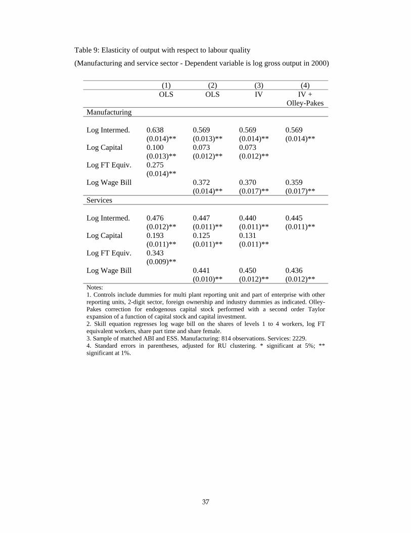
differences were robust to using value added instead of gross output. Second, in Table 9 we

look at the performance of the wage bill as a quality-adjusted employment figure. This is of

interest for, as Hellerstein and Neumark (2003) point out, wage bill is often available in

productivity studies whereas skill levels are not. We check the robustness of estimates of

output elasticities of labour, intermediate goods and capital. Column 1 is an OLS equation

with employment as full-time equivalents, as would be estimated with most standard firm-

level datasets, whereas column 2 shows the same but with log wage bill entered. The output

elasticities are in fact quite similar to those in Table 5 suggesting that in this sense the use of

the wage bill is adequate. Note that the elasticities in column 1 for intermediate goods and

capital are basically identical to our earlier maximum likelihood estimates that model the

quality of labour with skills and female share information. Thus the omission of these

characteristics has little impact on other estimates as found by Hellerstein and Neumark

(2003) and Hellerstein et al. (1999) for US manufacturing firms. However, an observation

of column in which wage bill is introduced instead of full-time equivalents, output appears

to be more responsive to labour quality whereas intermediate goods and capital become less

22

important, suggesting there may be other unobserved characteristics of labour that influence

productivity and are best reflected through wages.

Column 3 presents IV estimation results in which we instrument the log of wage bill with

the log of employment and shares for qualification levels, part timers and females.

Assuming, as one would do under competitive labour markets, that those characteristics

would only influence output through their impact on the quantity and quality of labour, this

would adjust for potential endogeneity of the wage bill regressor. Finally, column 4 uses

the Olley-Pakes method (Olley and Pakes, 1996) to control for potential endogeneity of the

capital stock variable. We did this by adding to the equation a squared polynomial in

capital and investment. It is easy to note that adjustments in columns 3 and 4 left the simple

OLS coefficients on the wage bill and other inputs unaffected. These results appear to

suggest that labour quality is generally poorly measured leading to a generic understatement

of labour’s role in driving output. Better employee data should be therefore obtained,

exploring alternative specifications for output which do not assume perfect substitutability

between types of labour. Further checks provided indications of positive interactions

between skills and capital, but our sample sizes did not provide the sufficient power to test

this against all possible interactions.

Assessing human capital spillovers

Our investigation of the role of human capital in driving firm-level productivity explores the

association between measures of human capital in the areas where firms are located and

their levels of outputs and wages. We address this question by estimating extended

production and wage regressions that also include local area characteristics, amongst them

the share of level 4 educated individuals who reside in the firm’s local authority or work in

it, according to 2001 Census figures available at that spatial level.17 Both measures are of

interest since it is not clear whether potential learning benefits might come from the local

employed workforce or local residents. The single-plant issue is important here, since if the 17 Local authority district – Unitary Authority (LADUA). Estimates for residents are also available for narrower spatial units such as wards and enumeration districts. We hypothesize that local authority is a relevant administrative boundary for the purposes of this analysis, although non administrative boundaries like travel to work areas (defined by ONS to capture 75% of workers to reside in the area boundaries) may capture

23

RU account for many LUs then the locality is not well defined. Thus we estimate

regressions for the full sample and the reduced sample of single-plant RUs to check this.

The top panel of Table 10 sets out the results for manufacturing, which correspond to

simple OLS regressions on all the coefficients included in our previous estimates but also

include indicators for whether LADUAs are in metropolitan areas and population density.18

Regardless of the specification and sample, the surrounding skill term is significantly

associated with higher productivity. Ceteris paribus, a firm located in an area with, say, 40

percent of the population with level 4 (e.g. degree), output will be 13.6 percent higher than

in an area with only 30 percent of population educated at that level. These estimates are

comparable to those obtained by Moretti (2002 and forthcoming) from large cross sections

of US manufacturing firms in 1980 and 1990. Wages are also observed to be higher in

firms located areas with higher skill density, as seen on columns 5 to 8, with very similar

qualitative and quantitative results.

The lower panel shows estimates for service sector firms. Recall that multi-plants are more

prevalent in services and this seems reflected in the estimates. When we use our full sample

we obtain insignificant estimated effects on productivity, but as we select single-plant firms

the estimates become comparable to those we found for manufacturing. It is interesting to

note that estimates of the impact of firm-level wages are approximately half in size, which

may be due to spillover rents accruing to employers or to the dampening effect of higher

skill abundance on wages.19

A number of points are worth noting. First, if firm location is endogenous then high

productivity firms might locate in areas of high skills for other unobserved, correlated

reasons, and hence the correlation between local skills and productivity would be spurious.

Thus we would expect the effects here to be an upper bound on outside influence. We try to

control for this through population density measures and region fixed effects.

this concept more adequately. As a result of this definition, TTWAs need to be continuously redefined as commuter patterns vary over time. 18 These are estimates of the production function with log gross value added as the regressor. 19 Sensitivity checks showed that excluding the internal qualification variables led to overestimation of the coefficient for surrounding skills. For the full sample of sectors and firms, a coefficient of 0.45 would become 0.49 (se=0.18) whereas for all sectors, single-plant firms, the coefficient moved from 1.06 to 1.15 (se=0.44).

24

Second, these estimated relationships reflect the equilibrium behaviour of individuals and

firms, which includes location decisions and investments in human capital by both sides.

Our results appear to confirm the existence of human capital externalities, which is stronger

than simply suggesting that areas with more skilled workers provide better opportunities to

firms because skills become cheaper (a pecuniary externality). If firms obtain a competitive

advantage in terms of additional learning by locating in areas with more skilled individuals,

they will revise their location up to the point where the costs incurred more than offset the

potential gains. If externalities are essentially constrained to a given physical area because

of transport and communication costs, the fixed resources that warrant better access to the

positive externality will capture the generated rents through higher land prices up to a point

in which the incentives to change location by firms disappear.

Third, the presence of externalities implies a market failure, for the benefits from investing

in human capital are never fully captured by those who make the investment effort.

Relative competitiveness in the different markets for capital, land, labour and products will

determine the distribution of such benefits. On the basis of that information, an economic

efficiency case for intervention could be made and Pigouvian taxes and subsides could be in

principle implemented to correct for the resulting market failures. It is important to note

that interventions of this type should always account for the mobility decisions of firms and

individuals. Efforts concentrated on particular localities or sectors may fail to achieve the

desired outcomes if there are, for example, strong incentives for individuals to acquire skills

in more subsidised areas only to move later to those areas in which they can most benefit

from the newly obtained skills.

6. Conclusions

This paper has shed new light into the association between workforce characteristics and

firm-level productivity in the UK. We used a unique matched data set with information on

the qualification attainment of firms’ workforce and standard input and performance

measures. This data set, despite its many limitations, has allowed us to investigate a series

of aspects which could only be previously inferred from individual-level wage data, thereby

forcing researchers to make considerable assumptions regarding competitiveness in labour

markets.

25

Regarding the three questions we started with our data suggest:

1. Firms with higher proportions of more educated, male and full time workers also

tend to be more productive. The magnitude of these effects substantially varies by

sector, and low level skills at the firm do not seem to have a statistically significant

effect on productivity in any of the regressions that we run. This echoes the findings

from wage equations which show zero or next to zero returns for those skills.

2. We cannot fully reject the hypothesis that skills are “under- or over-paid” relative to

inferred productivity differences. The same result broadly applies to gender-based

differences. Our data definitely show that firms employing a bigger proportion of

part-timers have higher relative productivity levels with respect to firms with more

full timers than their actual wage bills would indicate.

3. We find evidence consistent with for area-based, human capital externalities.

Of course, our results come with a number of caveats. First, concerning the sample

available, we have been only able to match a limited number of plants and firms and would

clearly like to achieve larger samples. Unless the sampling basis of the ESS is changed it is

hard to see how we can improve this however. Second, as in all non-experimental studies,

endogeneity is clearly an issue with regards to internal workplace characteristics and area

attributes. In particular, if firms locate in “good” areas which also have skilled workers

then the association between external skills and productivity is potentially spurious.

However, given that, to the best of our knowledge, we have not previously had any large-

scale plant level data with internal and external skills information, we believe our results to

be of interest. Furthermore, despite potential endogeneity problems, the comparative

analysis of wage and productivity estimates for internal workplace characteristics appears to

be worth the effort and may not be affected by bias in the individually estimated

coefficients.

26

References

Acemoglu, D. (1999), “Changes in Unemployment and Wage Inequality: An Alternative

Theory and Some Evidence”, American Economic Review, 89, pp. 1259-1278.

Acemoglu, D, and Angrist, J. (2001) “How Large are the Social Returns to Education?

Evidence from Compulsory Schooling Laws.” In NBER Macroeconomics Annual 2000,

Benn Bernanke and Kenneth Rogoff, eds. Cambridge: MIT Press.

Criscuolo, C., Haskel, J. and Martin, R. (2003). “Building the evidence base for

productivity policy using business data linking”, Economic Trends, 600, pp. 39-61.

Hawkes, D., (2003), “Report on Matching the Annual Business Inquiry to Learning and

Training at Work Survey and Employers Skills Survey”, CeRiBA working paper.

Haskel, J., Hawkes, D. and Pereira, S. (2003), “How much do skills raise productivity? UK

evidence from matched plant, worker and workforce data.” CeRiBA mimeo.

Hellerstein, J. and Neumark, D. (2003). “Production Function and Wage Estimation with

Heterogeneous Labor: Evidence from a New Matched Employer-Employee Data Set”.

NBER Working Paper.

Hellerstein, J., Neumark, D. and Troske, K. (1999). “Wages, Productivity, and Worker

Characteristicis”. Journal of Labor Economics, Vol. 17, No. 3, pp. 409-446.

IFF Research Ltd (2002) Employers Skills Survey 2001 Research Report, Department for

Education and Skills.

Manning, A. and Goos, M. (2003), “Lousy and lovely jobs: the rising polarization of work

in Britain,” CEP Discussion Paper, no. 604.

Martin, R. (2003). “Building the Capital Stock,” CeRiBA mimeo.

Moretti, E. (2002). “Human capital spillovers in manufacturing. Evidence from plant-level

production functions”, NBER Working Paper No. 9316.

Moretti, E. (forthcoming). “Workers’ education, spillovers and productivity: Evidence from

plant-level production functions”. American Economic Review.

Office for National Statistics (ONS), (2001). “Review of the Inter-Departmental Business

Register”, http://www.statistics.gov.uk/downloads/theme_commerce/IDBRB_v2.pdf

Olley, S. and Pakes, A. (1996). “The Dynamics of Productivity in the Telecommunications

Equipment Industry”, Econometrica, Vol. 64, No. 6, pp. 1263-1297.

27

Figure 1: Frequency of shares of workers educated to level 3 and above, by sector. Fr

actio

n

Share Level 3+

CDE:Manufacturing

0

.2

.4

.6F:Construction G:Trade and repairs

H:Hospitality

0

.2

.4

.6

I:Transport and communications K:Business Services

0 1MN:Education and Health

0 10

.2

.4

.6OPQ:Other services

0 1

Source: ESS-ABI matched sample.

28

Figure 2: Scatter plot of residuals from regression of log value added on inputs and industry

dummies against level 4 share residuals on industry dummies

Share Level4 residuals

Gross value added residuals Fitted values

-1 0 1

-1

0

1

Source: Employer Skills Survey and ABI. Note: Residuals are obtained from regressions of gross value added on firm level inputs and SIC92-2digit dummies and regression of share of level 4 workers also on industry dummies.

29

Table 1: Matching of ESS with ABI

Sample Sample size:

[ESS establishments]

Original ESS survey 27,032

ESS matched by ONS to IDBR 17,111

ESS-IDBR-ABI RU unambiguous matches 4,089

ESS-IDBR-ABI RU with valid GO, employment and GVA 3,199

Of which

Manufacturing CDE 814

Construction F 156

Wholesale, retail trade and repair G 766

Hotels and restaurants H 414

Transport and communications I 214

Business services K 485

Education and health services MN 184

Other services (OPQ) 166

Note: Summary of linkage between ESS and ABI reporting units (RU), leading to final estimation sample.

30

Table 2: Descriptive statistics, matched ESS-ABI sample

Manufacturing Services

Variable Mean Std. Dev. Mean Std. Dev.

Share Level 4 0.18 0.23 0.20 0.29

Share Level 3 0.19 0.25 0.21 0.29

Share Level 2 0.36 0.34 0.39 0.39

Share Level 1 0.09 0.23 0.07 0.20

Log Employment 5.58 1.32 7.10 2.59

Female share 0.27 0.19 0.51 0.23

Part Time Share 0.06 0.09 0.36 0.28

Log Wages/ Emp 3.09 0.38 2.58 0.66

Log GO/ Emp 4.50 0.69 4.00 0.99

Log GVA/ Emp 3.45 0.66 2.96 0.84

Log Capital/Emp 3.95 0.96 3.33 1.15

Log Interm/ Emp 3.94 0.88 3.23 1.40

In multi-plant RU 0.57 0.49 0.79 0.40

In multi-RU ent. 0.12 0.32 0.25 0.43

Foreign 0.21 0.41 0.08 0.28 Observations: Manufacturing (814), Services (2229)

Note: GVA=gross value added, GO=gross output.

31

Table 3: Productivity and other measures by skill intensity of the RU (Level 3+)

Quintiles of Level 3+ share

1 2 3 4 5

Full

sample

Share Level 3 or higher 0.005 0.107 0.276 0.655 0.977 0.403

Share Level 4 0.002 0.042 0.126 0.354 0.469 0.199

Log unit GVA 2.920 2.956 3.188 3.231 3.238 3.106

Log Unit Wage Bill 2.500 2.564 2.790 2.909 2.907 2.734

Log Unit Capital 3.215 3.326 3.658 3.646 3.618 3.492

Log Unit Intermediate Goods 3.442 3.530 3.557 3.426 3.300 3.451

Female Share 0.453 0.456 0.392 0.422 0.447 0.434

Part Time Share 0.343 0.332 0.213 0.212 0.236 0.267

Foreign 0.068 0.114 0.163 0.134 0.119 0.119

Multi-plant RU 0.779 0.772 0.661 0.697 0.748 0.731

Share Level 4: LADUA–population 0.198 0.192 0.196 0.213 0.237 0.207

Share Level 4: LADUA–workforce 0.224 0.219 0.222 0.241 0.266 0.235

Log Employment 7.176 7.380 6.167 6.053 6.377 6.631

Observations 647 636 637 640 639 3199

Notes:

(1) Cross-establishment average of listed firm-level characteristics, by establishment position in

distribution of skill intensity, as measured by share of employees with level 3 or higher.

(2) LADUA denotes Local Authority District-Unitary Authority.

32

Table 4: Share of females, part timers and level 3 and 4 by sector

Sector Log GVA/

Emp

Female

share

Part-time

share

Share with

qualification

over level 3

CDE: Manufacturing-Production 3.45 0.27 0.06 0.37

F: Construction 3.35 0.13 0.04 0.52

G: Trade and repairs 2.91 0.51 0.40 0.28

H: Hospitality 2.68 0.58 0.53 0.35

I: Transport and Communications 3.29 0.25 0.11 0.33

K: Business Services 3.37 0.49 0.21 0.60

MN: Private Education and Health 2.51 0.76 0.44 0.62

OPQ: Other services 2.82 0.52 0.39 0.43

Total 3.10 0.44 0.27 0.43

33

Table 5: Estimation of firm-level productivity and wage functions

All firms Manufacturing Services

Productivity Wage Productivity Wage Productivity Wage

Coef. Std. Err. Coef. Std. Err. Coef. Std. Err. Coef. Std. Err. Coef. Std. Err. Coef. Std. Err.

Ln Labour Quality 0.336 0.014 0.291 0.027 0.352 0.017 Ln Capital 0.149 0.016 0.092 0.020 0.190 0.022 Ln Intermediate 0.526 0.018 0.631 0.029 0.472 0.024 Foreign 0.072 0.021 0.135 0.031 0.036 0.023 0.104 0.031 0.093 0.033 0.217 0.039 Multi-plant -0.052 0.018 0.045 0.022 -0.006 0.018 0.053 0.025 -0.091 0.028 -0.047 0.036 Multi RU enterprise -0.033 0.024 0.016 0.058 -0.022 0.026 0.033 0.033 -0.036 0.032 -0.028 0.073 Part Time Share -0.509 0.102 -1.205 0.119 -0.297 0.274 -1.023 0.162 -0.521 0.109 -1.197 0.127 Female Share -0.271 0.110 -0.337 0.111 -0.311 0.181 -0.347 0.112 -0.277 0.124 -0.369 0.139 Share Level 4+ 0.155 0.091 0.423 0.049 0.497 0.208 0.343 0.053 0.127 0.094 0.478 0.065 Share Level 3 0.020 0.044 0.120 0.033 0.139 0.130 0.188 0.051 0.025 0.046 0.109 0.042 Share Level 2 0.014 0.033 0.051 0.025 -0.021 0.081 0.060 0.035 0.037 0.035 0.055 0.032 Share Level 1 0.037 0.046 0.044 0.038 -0.153 0.107 0.032 0.048 0.110 0.058 0.057 0.051 Log likelihood

Observations

-2381.48

3199

-68.33

814

-2010.27

2229 Note: Joint maximum likelihood estimation of production function (log gross output) with labour quality term and wage equation (log wage bill per employee), with standard errors (in italics) adjusted for clustering at the reporting unit level. Observations are ESS establishments matched to ABI reporting units (single and multi-plant reporting units). Coefficients on part-time, female and qualification shares in productivity column denote relative productivity (implied wage returns) with respect to baseline of male full-time workforce with no qualifications.

34

Table 6: Implied returns to level 4 qualifications from firm-level productivity regressions

Sectors

Productivity

measure

Establishment

type All Manufacturing Services

Gross output All 0.155 (0.091)

0.497 (0.208)

0.127 (0.094)

Gross output Single-plant RUs

0.476 (0.241)

0.507 (0.329)

0.491 (0.317)

Gross Value Added All 0.138

(0.068) 0.571

(0.208) 0.131

(0.076) Gross Value Added

Single-plant RUs

0.208 (0.175)

0.704 (0.333)

0.176 (0.225)

Notes: 1. Estimates based on maximum likelihood estimates of coefficient for Level 4 share term in quality of

labour term, denoting implied return to Level 4 qualification relative to baseline of no qualifications. 2. Standard errors within parentheses, adjusted for RU-level clustering

35

Table 7: Comparison of productivity-implied returns for workforce attributes and observed

wage differentials

Establishments in Single and Multi-Plant RUs

All sectors Manufacturing Services

Difference p-value Difference p-value Difference p-value

Part time share 0.69 0.00 0.73 0.01 0.67 0.00

Female share 0.06 0.61 0.04 0.83 0.09 0.55

Share Level 4 -0.27 0.00 0.15 0.43 -0.35 0.00

Share Level 3 -0.10 0.02 -0.05 0.69 -0.08 0.08

Observations 3199 814 2299

Establishments in Single-Plant RUs

All sectors Manufacturing Services

Difference p-value Difference p-value Difference p-value

Part time share 0.74 0.00 0.43 0.49 0.68 0.00

Female share -0.15 0.36 -0.29 0.22 -0.06 0.74

Share Level 4 -0.04 0.84 0.19 0.54 -0.17 0.53

Share Level 3 -0.03 0.98 0.13 0.61 -0.01 0.93

Observations 859 347 452 Notes:

1. Equality of implied and observed returns to workforce characteristics, based on maximum likelihood estimates as in Table 7.

2. Difference=(Productivity-implied return)-(Wage-implied return). P-value follows from test of the null hypothesis of difference being zero. In the case of part-time and females, the returns are negative. So a positive difference indicates that although productivity is lower, wages are lower still. In the case of skills, whose returns are positive, a negative difference indicates that although productivity is higher, wages are higher still.

3. Dependent varibles for productivity, log gross output, for wages log wages per employee.

36

Table 8: The Contribution of skills in accounting for differences in productivity

Log gross output per employee Share level 4

10th percentile 2.99 0.0

90th percentile 5.30 0.7

Memo items

Implied return (coefficient) 0.155

Output elasticity of quality of labour 0.336

Calculations

Log point difference in output of firm at p90 relative to p10 due

to skills:

N=α.{ln(1+θ.Q(SL4|p90))- ln(1+θ.Q(SL4|p10)) 0.015

Actual log point labour productivity difference

D=Q(LabProd|p90)- Q(LabProd|p10) 2.310

Fraction due to skills (N/D) 0.0065 (0.65%)Notes:

(1) Full sample of single and multi-plant RUs. (2) Comparison based on simplest comparison framework with zero-levels for PT-share, Female

Share and Level 2 and 3 shares.

37

Table 9: Elasticity of output with respect to labour quality

(Manufacturing and service sector - Dependent variable is log gross output in 2000)

(1) (2) (3) (4) OLS OLS IV IV +

Olley-Pakes Manufacturing Log Intermed. 0.638 0.569 0.569 0.569 (0.014)** (0.013)** (0.014)** (0.014)** Log Capital 0.100 0.073 0.073 (0.013)** (0.012)** (0.012)** Log FT Equiv. 0.275 (0.014)** Log Wage Bill 0.372 0.370 0.359 (0.014)** (0.017)** (0.017)** Services Log Intermed. 0.476 0.447 0.440 0.445 (0.012)** (0.011)** (0.011)** (0.011)** Log Capital 0.193 0.125 0.131 (0.011)** (0.011)** (0.011)** Log FT Equiv. 0.343 (0.009)** Log Wage Bill 0.441 0.450 0.436 (0.010)** (0.012)** (0.012)** Notes: 1. Controls include dummies for multi plant reporting unit and part of enterprise with other reporting units, 2-digit sector, foreign ownership and industry dummies as indicated. Olley-Pakes correction for endogenous capital stock performed with a second order Taylor expansion of a function of capital stock and capital investment. 2. Skill equation regresses log wage bill on the shares of levels 1 to 4 workers, log FT equivalent workers, share part time and share female. 3. Sample of matched ABI and ESS. Manufacturing: 814 observations. Services: 2229. 4. Standard errors in parentheses, adjusted for RU clustering. * significant at 5%; ** significant at 1%.

38

Table 10: The impact of surrounding skills on productivity and wages (OLS estimates) (1) (2) (3) (4) (5) (6) (7) (8) Manufacturing Log GVA Log GVA Log GVA Log GVA Log Wages Log Wages Log Wages Log Wages Share level 4+ 0.294 0.310 0.303 0.311 0.262 0.192 0.258 0.185 (0.131)* (0.178) (0.130)* (0.180) (0.057)** (0.098)* (0.056)** (0.098)* Share level 3 0.210 0.211 0.211 0.221 0.193 0.213 0.193 0.219 (0.109) (0.152) (0.109) (0.151) (0.053)** (0.082)* (0.053)** (0.082)* Share level 2 0.052 0.229 0.061 0.241 0.056 0.114 0.060 0.121 (0.069) (0.108)* (0.069) (0.109)* (0.035) (0.060) (0.036) (0.060) Share level 1 -0.028 0.161 -0.021 0.162 0.031 0.086 0.034 0.086 (0.091) (0.138) (0.091) (0.139) (0.049) (0.079) (0.049) (0.079) Share level 4+ in LADUA 1.243 1.366 0.638 0.988 (Adult resident population) (0.323)** (0.548)* (0.234)** (0.379)* Share level 4+ in LADUA 1.354 1.367 0.855 1.154 (Workforce) (0.358)** (0.610)* (0.254)** (0.393)** Single plant only? – Obs No – 814 Yes -347 No - 814 Yes -347 No - 814 Yes -347 No - 814 Yes -347 Services Share level 4+ 0.220 0.334 0.218 0.330 0.449 0.558 0.444 0.548 (0.067)** (0.170) (0.067)** (0.173) (0.055)** (0.135)** (0.057)** (0.136)** Share level 3 0.055 0.045 0.055 0.047 0.108 0.214 0.117 0.214 (0.057) (0.171) (0.057) (0.171) (0.044)* (0.121) (0.044)* (0.121) Share level 2 0.010 0.143 0.010 0.147 0.061 0.124 0.066 0.127 (0.044) (0.127) (0.044) (0.128) (0.035) (0.095) (0.036) (0.095) Share level 1 0.088 0.263 0.089 0.281 0.042 -0.020 0.061 -0.007 (0.061) (0.239) (0.061) (0.240) (0.047) (0.164) (0.048) (0.165) Share level 4+ in LADUA 0.231 1.483 0.355 0.658 (Adult resident population) (0.234) (0.750) (0.183) (0.458) Share level 4+ in LADUA 0.321 1.607 0.552 0.979 (Workforce) (0.266) (0.773)* (0.175)** (0.501) Single plant only? – Obs. No- 2229 Yes-452 No- 2229 Yes-452 No- 2229 Yes-452 No- 2229 Yes-452 Notes: Estimates for separate linear regressions on all arguments. Robust standard errors in parentheses, adjusted for clustering at the LADUA level. * significant at 5%; ** significant at 1%. Other controls include log employment and capital, region and sector dummies, foreign, multi plant and multi RU enterprise dummies, female and part time share, metro area indicator and log population density in LADUA.

39

Appendix: Deriving firm-level qualifications data from the ESS

As explained in the main text, the ESS does not ask employers to report directly on

the proportion of workers with a given level of educational attainment. Instead,

proportions are only directly available for occupational groups. In a second step,

respondents are asked to state the most frequent level of educational attainment within

the firm for each occupational group. We construct an estimate of firm-level

proportion of workers with a given qualification by averaging qualification responses

across occupation, using the occupation shares as weights. This implicitly assumes

that within occupations, the distribution of qualification attainment is strongly

unimodal.

The following test reproduces the relevant sections of the questionnaire.

ASK ALL

A1 I’d like to ask you to break down your workforce into nine specific categories. These categories are… [LIST CATEGORIES WITH EGs]

Would you like to record staff details as a percentage or as actual numbers of staff? Approximately, what proportion of staff at this establishment are employed as/How many of your staff are employed as… ? READ OUT

Managers and senior officials e.g. directors, senior government officials, senior police officers _______% Professional occupations e.g. professional engineers, scientists, accountants, teachers, solicitors, architects, librarians _______% Associate Professional and technical occupations e.g. laboratory technicians, junior police officers, design and media professionals, nurses, artists _______% Administrative and secretarial occupations e.g. clerks, computer operators, secretaries, telephonists _______% Skilled trades occupations e.g. fitters, electricians, farmers, computer engineers, bricklayers _______% Personal service occupations e.g. catering staff, hairdressers, domestic staff, caretakers _______% Sales and customer service occupations Till operators, telesales staff, call centre staff, market traders _______% Process, plant and machine operatives e.g. machine operators, drivers, scaffolders, assembly line workers _______% Elementary occupations e.g. labourers, cleaners, security guards, postal workers, bar staff, shelf fillers, waiters _______% 100%

40

FOR EACH OCCUPATION GROUP MENTIONED AT QD1

D1a Thinking about your current workforce, what is the most common level of qualification amongst your ….(OCCUPATION AT QD1) ?

PROMPT IF NECESSARY. Would you say that they typically have ….? READ OUT. SINGLE CODE ONLY

1 2 3 4 5 6 7 8 9 Level*Higher level of qualification such as degree or equivalent (e.g. NVQ level 4/ Nursing/ HND/ HNC/ Higher diploma)

1 1 1 1 1 1 1 1 1 4+

Intermediate level of qualification such as A levels or equivalent (e.g. NVQ level 3/ BTEC National/ /OND/ City and Guilds Advanced Craft)

2 2 2 2 2 2 2 2 2 3

Basic level of qualification such as G.C.S.Es or equivalent (NVQ level 2/ O levels/ BTEC first or general diploma/ Intermediate GNVQ/ City and Guilds Craft)

3 3 3 3 3 3 3 3 3 2

Lower level of qualification such as NVQ Level 1 or equivalent (BTEC first or general certificate/ basic vocational training/ RSA/ Foundation GNVQ)

4 4 4 4 4 4 4 4 4 1

Other qualifications (SPECIFY) 5 5 5 5 5 5 5 5 5 0 None V V V V V V V V V 0 * Last column not included in questionnaire form, included to indicate correspondence with English classification of qualifications