1 Skyline Collision Energy Optimization As of version 0.6, Skyline now supports a rich user interface and fully automated pipeline for predicting and optimizing SRM instrument parameters like collision energy (CE) and declustering potential (DP). This tutorial focuses on CE optimization, but the same principles apply to DP optimization, and could eventually apply to other parameters, such as cone voltage. So far this functionality has been thoroughly tested for Thermo, Applied Biosystems and Waters instruments, and we are working with Agilent on a fix to their collection software. In most cases, the default method in Skyline of assigning CE values to transitions sacrifices very little peak area to full, empirical optimization of each transition separately. We are working on publishing the data set we collected to support this conclusion, but Skyline provides ample support for testing it yourself, or just performing per-transition CE optimization when you feel the need. The default method in Skyline for calculating CE values is to use a linear equation of the form: CE = slope * (precursor m/z) + intercept Each charge state is allowed to have a separate equation. As a result of our recent experimentation, we have derived new linear equations to calculate CE for “Thermo TSQ Vantage”, “Thermo TSQ Ultra” and “ABI 4000 QTrap” instruments for both charge 2 and 3. We feel these are the most thoroughly measured equations of their kind to date, and recommend their use over the equations available in previous versions of Skyline under the names “Thermo” and “ABI”. In this tutorial, we will cover how to use Skyline both to derive your own linear equations for CE and to perform empirical, per-transition optimization. Getting Started To start this tutorial, download the following ZIP file: https://skyline.gs.washington.edu/tutorials/OptimizeCE.zip Extract the files in it to a folder on your computer, like: C:\Users\brendanx\Documents This will create a new folder: C:\Users\brendanx\Documents\OptimizeCE It will contain all the files necessary for this tutorial. Open the file CE_Vantage_15mTorr.sky in this folder, either by double-clicking on it in Windows Explorer, or by choosing Open from the File menu in Skyline.
Transcript
1
Skyline Collision Energy Optimization
As of version 0.6, Skyline now supports a rich user interface and fully automated pipeline for predicting
and optimizing SRM instrument parameters like collision energy (CE) and declustering potential (DP).
This tutorial focuses on CE optimization, but the same principles apply to DP optimization, and could
eventually apply to other parameters, such as cone voltage. So far this functionality has been
thoroughly tested for Thermo, Applied Biosystems and Waters instruments, and we are working with
Agilent on a fix to their collection software.
In most cases, the default method in Skyline of assigning CE values to transitions sacrifices very little
peak area to full, empirical optimization of each transition separately. We are working on publishing the
data set we collected to support this conclusion, but Skyline provides ample support for testing it
yourself, or just performing per-transition CE optimization when you feel the need. The default method
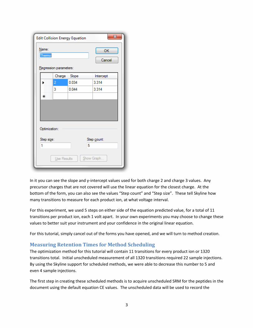
in Skyline for calculating CE values is to use a linear equation of the form:
CE = slope * (precursor m/z) + intercept
Each charge state is allowed to have a separate equation.
As a result of our recent experimentation, we have derived new linear equations to calculate CE for
“Thermo TSQ Vantage”, “Thermo TSQ Ultra” and “ABI 4000 QTrap” instruments for both charge 2 and 3.
We feel these are the most thoroughly measured equations of their kind to date, and recommend their
use over the equations available in previous versions of Skyline under the names “Thermo” and “ABI”.
In this tutorial, we will cover how to use Skyline both to derive your own linear equations for CE and to
perform empirical, per-transition optimization.
Getting Started To start this tutorial, download the following ZIP file:
471.2562 484.3242 20.3 15.03 19.03 1 DGGIDPLVR gi|129823|Lactoperoxidase y4 You can see that the CE values in the third column differ among transitions of the same precursor.
Skyline has chosen the CE value that produced the maximum measured peak area for each transition.
12
Conclusion There is certainly more to learn about CE optimization, and we encourage you to watch for the article on
our recent investigation into its use and benefits. Hopefully this tutorial will be enough to get you
started on using Skyline for your CE optimization needs. If your instrument is not now explicitly covered
by name in the Transition Settings list of linear equations for CE calculation, you may want to run your
own tests to ensure you are using a linear equation that calculates the best CE values as accurately as
possible. If you are performing SRM experiments with many peptides in charge states not covered by an
existing equation, you probably will want to calculate new equations for those charge states. This
tutorial should have provided you with the tools you will need in these cases. We hope you will use