SLAC-127 UC-32 W=C) DIRECT EMULATION OF CONTROL STRUCTURES BY A PARALLEL MICRO-COMPUTER VICTOR R. LESSER* STANFORD LINEAR ACCELERATOR CENTER STANFORD UNIVERSITY Stanford, California 94305 PREPARED FOR THE U. S. ATOMIC ENERGY COMMISSION UNDER CONTRACT NO. AT(04-3)-515 October 1970 Reproduced in the USA. Available from the National Technical Information Service, Springfield, Virginia 22151. Price: Full size copy $3.00; microfiche copy $ .65. * The research was carried on while the author was a NSF graduate fellow and partially supported under NSF2-FCZ-708-94140, AT(043)326, P.A.23.
Transcript
SLAC-127 UC-32 W=C)
DIRECT EMULATION OF CONTROL STRUCTURES
BY A PARALLEL MICRO-COMPUTER
VICTOR R. LESSER*
STANFORD LINEAR ACCELERATOR CENTER STANFORD UNIVERSITY
Stanford, California 94305
PREPARED FOR THE U. S. ATOMIC ENERGY
COMMISSION UNDER CONTRACT NO. AT(04-3)-515
October 1970
Reproduced in the USA. Available from the National Technical Information Service, Springfield, Virginia 22151. Price: Full size copy $3.00; microfiche copy $ .65.
* The research was carried on while the author was a NSF graduate fellow and partially supported under NSF2-FCZ-708-94140, AT(043)326, P.A.23.
ABSTRACT
This paper is a preliminary investigation of the organization of a parallel
micro-computer designed to emulate a wide variety of sequential and parallel
computers. This micro-computer allows tailoring of the control structure of
an emulator so that it directly emulates (mirrors) the control structure of the
computer to be emulated. An emulated control structure is implemented through
a tree type data structure which is dynamically generated and manipulated by
six primitive (built-in) operators D This data structure for control is used as a
syntactic framework within which particular implementations of control concepts,
such as iteration, recursion, co-routines, parallelism, interrupts, etc., can be
easily expressed. The major features of the control data structure and the
primitive operators are: 1) once the fixed control and data linkages among
processes have been defined, they need not be rebuilt on subsequent executions
of the control structure; 2) micro-programs may be written so that they execute
independently of the number of physical processors present and still take advan-
tage of available processors; 3) control structures for I/O processes, data-
accessing processes, and computational processes are expressed in a single uniform framework. This method of emulating control structures is in sharp
contrast with the usual method of micro-programming control structures which
handles control instructions in the same manner as other types of instructions,
e.g., subroutines of micro-instructions, and provides a unifying method for the
efficient emulation of a wide variety of sequential and parallel computers.
. . . - 111 -
ACKNOWLEDCEMENI’S
I wish to express my sincere thanks to Professor Wdliam Miller whose
constant support and encouragement of my research efforts have made possible
the successful completion of this paper. I would also like to thank Professor Ed Davidson for his detailed reading.and criticisms of this paper, and Dr. Harry
Saal and Professor William McKeeman for their encouragement of my research
efforts and the many fruitful discussions I had with each. Thanks especially to
my friends and fellow graduate students Lee Erman and Bill Riddle who have had
to suffer through an uncountable number of rewrites and discussion of’this.paper.
- iv -
TABLE OF CONTENTS
Page
I. INTRODUCTION. .......................
A. Traditional Micro-Computer Architecture ..........
B. Variable Control Structure as the Basis of a
Micro-Computer Architecture ...............
II. MICRO-COMPUTER ARCHITECTURE. .............
III. MICRO-PROCESSOR SUBSYSTEM. ...............
IV. STRUCTURE BUILDING LANGUAGE (SBL). ...........
A. Control Data Structure ...................
B. Use of the Six SBL Macro Types ..............
C. Format of SBL Macro Calling Sequence ...........
D. Subsystem Command Macros ................
E. Structure Building Macros .................
1. Sequential Control Structures ..............
2. Nonsequential Control Structures ............
3. Tree Structured Addressing. ..............
4. Synchronization, and Control and Data Linkage Among Processes ...................
V. INTEGER FUNCTION LANGUAGE (IFL) .............
A. Format and Sequencing of IFL Instructions ..........
B. Built-In Arithmetic Operations ...............
C. Side Effects in IFL. ....................
D. Pseudo-Functional Units ..................
VI. FORMAT OF SBL MACROS ..................
A. Data-Descriptor Macro ..................
B. Selection Macro ......................
C. Iteration Macro ......................
D. Instruction and Hierarchical Macros. ............
2. Micro-Computer subsystems (modules) . . . . . . . . . . . . . 5 3. Micro-Processor subsystem’s organization . . D . . . . . . m . 12 4. The control data structure for an emulator of a von Neumann
In the past few years, both the size and diversity of the class of problems
being submitted to computers for solution has significantly increased. The
programming of many of these new problems on a computer with a von Neumann
organization can be very complex and, additionally, can result in programs which
execute inefficiently. A significant part of these difficulties can be attributed to
the “degree of complexity” of the transformation from the representational
framework within which the programmer develops an algorithm (e.g., ALGOL,
LISP, Graph Model, etc.) to the representational framework of a von Neumann
computer within which the algorithm is executed. The complexity of transfor-
mation between these two levels of representation thus makes it difficult to con-
struct an automatic mapping between levels which is both quick and efficient.
The perception of this problem has led to the development of computers whose
organizations are optimized for either a particular subset of or a higher level
language for the problem class 0 Examples of such machine languages should
include those of the B5500 ’ for ALGOL, ILLIAC IV 2 for processing of array
structured data, Abram’s APL machine, 3 Melbourne and Pugmire’s FORTRAN4
machine, etc D Since these represent a broader class of languages than what is
usually meant by machine language, we will refer to them as intermediate
machine languages (IML’s) s This tailoring of IML to a specific h)igher level language
is accomplished by incorporating primitive operators in the IML which directly mirror
operations in the higher level language (e. g D , recursion in ALGOL is directly mirrored
through stack operations in B5500) D Thus, bythetailoringof amachine’sorganization
more closely to a particular user representational framework, the mapping be-
tween levels is simpler and results in more efficient program execution.20
In parallel with the development of problem oriented computers, there has
been an effort toward providing a systematic and flexible approach to the hard-
ware design of a specific computer a This effort has led to the development of
micro-computers, e.g., 360/40, 5 . with read-only control memories programmed
to emulate a specific von Neumann type computer.
Recently, there has been an attempt to integrate both of these new directions
in computer architecture (machine organizations designed for specific applica- tions and micro-computers) by attaching to the micro-computer writeable
control memories D Thus, it is intended that through the ability to modify
dynamically the control memory of a micro-computer, a wide range of machine
languages of different computer organizations (IML) can be efficiently emulated
on a single micro-computer. However, it is the author’s contention that this
goal cannot be realized by existing micro-computers.
-l-
A. Traditional Micro-Computer Architecture
Existing micro-computer architectures are still oriented toward the design
of von Neumann type computers rather than a systematic approach to the emu-
lation of a wide variety of different sequential and parallel intermediary machine
languages.
The program structure of an IML emulator, in a conceptual sense, is seen
in Fig. 1.
FIG. l--Conceptual structure of an emulator.
The “control process”, which represents the control structure* of the com-
puter to be emulated, activates the “decoding process” with data that identifies
the next instruction(s) of the emulated computer to be executed; the “decoding
process ” analyzes the instruction(s) to be executed so as to determine the
semantic routine(s), together with its (their) appropriate calling sequence(s),
whose activation will perform the semantics of the emulated instruction(s).
After the appropriate semantic routine(s) has (have) been executed, the flow of
control returns to the control process which, based on the results of executing
the decoding process and the semantic routine(s), selects the next instruction(s)
to be emulated.
* The control structure of a computer consists of the set of rules used to define the sequencing of the instructions of the computer.
-2-
The organizations of existing micro-computers when applied to the emulation
of unanticipated IML’s do not reflect this conceptualization of the structure of
an emulator, but rather provide a simple, uniform framework for the coding of
an emulator. In these machines, the semantics of micro-instructions are gen-
erally realized by a short parallel sequence of register transfers, and the control
for sequencing among micro-instructions is sequential and based on simple con-
ditional transfer commands. There are no features in the language that distin-
guish the coding of the control process from that of the decoding process or the
semantic routines, nor the relationship, for instance, between the control process
and the decoding process. An emulator expressed in this type of micro-computer
langusge ‘la a q implements machine instructions as a subroutine of micro-
instructions”. 6 Thus, due to the simplicity of micro-computer languages and
their paucity of control commands, the structure of the emulated computer is
not directly observable in the structure of its emulator. The key to efficient
emulation is just this missing ability to directly mirror the control structure,
instruction formats, and primitive data-accessing operations of an IML in the corresponding control structure, instruction formats and primitive data-accessing
operations of its emulator. In particular, a control action by an instruction in
the IML program being emulated should be directly mirrored in a modification
of the control structure of the emulator.
Thus, the current approach to the design of a micro-computer which stresses
simplicity is not unreasonable if the micro-computer is going to emulate computers
and IML’s that have a simple sequential control and simple instructions. But,
IML’s that are tailored for a particular subset of a higher level language for a
problem class are, in a sense by their very purpose, not simple since the com-
plexity of the higher level language is imbedded in the semantics of the IML’s
instructions and control structure. If the current trend in higher level languages
is maintained, these problem or procedure oriented IML’s will have increasingly more sophisticated control structures employing such control concepts as
recursion, co-routines, parallelism, etc., and, likewise, their instructions
will directly operate on increasingly more complex data structures, e.g., lists, trees, arrays, etc. Therefore, the current structure of existing micro-computers
is inadequate for the task of effectively emulating the wide range of such inter-
mediary languages, just as a von Neumann computer in comparison with the
B5500 does not efficiently execute ALGOL.
-3-
B. Variable Control Structure as the Basis of a Micro-Computer Architecture
The micro-computer architectural design to be presented in this paper is
based on the idea that the program structure of an emulator written in this
micro-computer should reflect the structure of an IML that is being emulated.
It is felt that the key to accomplishing this mirroring process between IML and
its emulator lies in the control structure of the micro-processor. Thus, the
main emphasis in the design to be presented here is to incorporate a very general
control structure in the micro-processor,
The approach conventionally used to design a micro-processor with a
powerful control structure is first to develop a basic machine language having
a well-defined set of instructions and a simple sequential control structure, and
then add instructions and facilities (such as subroutine call instruction, a stack
for parameter passage, a fork-join instruction, etc.) for structuring complex
sequential and parallel processes. This is not the approach taken here. Instead,
the approach is to develop a micro-language specifically designed for the task of
dynamically constructing control structures a This control structure definition
language, called the Structure Building Language (SBL) , is used to dynamically
define a wide range of particularized control structures through the generation
of a data structure for control. The control data structure acts as a syntactic
framework within which dynamic and static control and data environment inter-
relationships among processes can be expressed. The control structure of this
micro-computer can then be dynamically tailored (through the SBL) into a form
which is most suitable for the emulation of a particular LML. An emulator
programmed in this micro-computer, as will be seen later, works in a fashion
similar to the process of dynamic compilation or run-time macro expansion.
This method of emulation differs radically from the conventional form of emulation consisting of a sequence of calls to sub-routines of micro-instructions.
The variable nature of the control structure of this micro-computer dis-
tinguishes its architecture (from the viewpoint of form and complexity) from
existing micro-computer architecture e It is felt that a variable control structure
micro-computer provides a unifying approach to the emulation of an extremely
wide variety of computer organizations and IML’s. The goals of this micro-
computer design are to be able to:
1. Emulate efficiently a wide class of both sequential and parallel
LISP machines, computational graph models, etc.) D
-4-
2. Program an emulation in a simple and uniform manner, such
that the dynamic program structure of an emulator reflects
the architecture of the computer it emulates.
3. Incorporate easily and efficiently a changing array of hardware
arithmetic units (e.g. , square root, inner product, etc.) I/O
devices and memory units (e.g., associative memory, bit
slice memory, etc .) o
Micro-Computer
Micro-Processor
I f n
I III II
FIG. 2--Micro-Computer subsystems (modules).
-5-
II. MICRO-COMPUTER ARCHITECTURE
The micro-computer architecture, as pictured in Fig. 2, can be character-
ized in terms of three basic hardware subsystems. The first subsystem is
composed of an arbitrary set of functional units. Each of these units can be
independently activated and can have an arbitrary number of inputs and outputs,
where that number need not be fixed but may be data dependent. A functional unit could be a floating point multiplier or, more generally, an arbitrary input/
output device. This more general usage of a functional unit is a natural conse-
quence of imposing restrictions neither on the size (or form) of the input and
output data sets of a unit nor on the sequencing between units.
The second subsystem is a memory. This memory is bit-addressable and can be activated either to store or retrieve an arbitrary length string of bits.
This memory holds the program that is going to be emulated, and additionally,
serves as a storage buffer for communication between the functional unit sub-
system and the micro-processor subsystem. Other types of memory organiza- tions, such as word-oriented, bit-slice, associative, etc., can also be included
in the system’s architecture by making them function units.
The third subsystem, which is the major innovation in this micro-computer architecture, is a micro-processor that controls the dynamic interactions
between the other two subsystems and among functional units. The programmable nature of the control unit of the micro-processor subsystem allows the tailoring
of both the hardware and software of this architecture to various problems. The hardware tailoring involves the addition of specialized functional units which
carry out operations commonly used in the problem class (e.g., floating-point
multiplier bit-slice memory, etc.) to the functional unit subsystem or addition of more parallelism in the micro-processor subsystem. The variable nature of the control unit of the micro-processor subsystem, as will be discussed later,
allows these hardware modifications to be incorporated without modification to
the language of the micro-processor. In order to emulate a computer using this system, the program which is
to be run on the emulated computer is stored bit-wise in the memory subsystem
in the same order as it would be stored in the emulated computer% memory.
The micro-processor must then perform the following tasks: (1) fetch from the
memory subsystem the instruction(s) of the emulated computer which is (are) to
-6-
be executed in the next step; (2) analyze this (these) instruction(s) in order to
generate the appropriate sequence of functional unit activations which will perform
the computations specified by the instruction(s). In addition, the sequence of
functional unit activations must be coupled with accesses and stores to the
memory subsystem so as to provide the input and output data set for each unit.
This sequence of functional activations may result in concurrent operation of
functional units or a pipelining of functional units.
The major focus of the rest of the paper will be on the organization of the
control unit of micro-processor subsystem, especially the syntax and semantics
of the SBL.
-7-
III. MICRO-PROCESSOR SUBSYSTEM
The main orientation in the design of this micro-computer, as stated in the
introduction, is to incorporate a variable control structure definitional facility
into the hardware of its processor. This design emphasis has led to a micro-
processor that contains two basic classes of instructions. One class of micro-
instructions, called the Structure Building Language (SBL), is used to construct
dynamically the control structure of an emulator while the other class, called the Imerger Function Language (IFL), is used to compute address arithmetic
functions e
The SBL dynamically defines an emulator’s control structure through the
generation of a data structure for control. The basis of the syntax and semantics
of the SBL is a fixed set of definitional templates that define particular types
(forms) of control structures. An SBL statement (macro) specifies one of the
fixed set of templates together with a set of IFL address arithmetic functions. Each definitional template represents a parameterized model of a basic control
concept, e-g,, iteration, selection, hierarchy, synchronization, etc. The
specification of particular values for the parameters of the template defines a
particular instance of a basic control concept. These values are computed by
the IFL address arithmetic functions specified in the SBL macro. A call to an
IFL program results in the generation of either an integer value or a sequence of
interger values that are then used in the expansion or execution of a macro. The
expansion of a definitional template results in the generation of a structure which
contains all the state information necessary to model the execution of this par-
ticular instance of the control concept. More complex control structures are
constructed through the expansion of a sequence of these definition templates.
The binding of parameters to the SBL macro is under the explicit control of other
SBL statements D Similarly, the expansion of SBL macros and later execution is
explicitly programmable in the SBL. This ability of the SBL to define dynamically
the sequencing of other SBL statements is the key to the control structure defi- nitional facility of the micro-processor.
The SBL consists of six types of macro bodies (definitional templates): data-
control (C) D The first two types of macro bodies are called subsystem command
macros while the remaining four are called structure building macros. The
subsystem command macros specify the interaction between the functional unit
-8-
subsystem and the memory subsystem. Only these two macros actually produce
computational results through the action of functional units. More complex
computational processes are constructed through the execution of a sequence of
structure building macros that use as their basic building block calling sequences
to subsystem command macros. When the basic building blocks are just data-
descriptor macro calling sequences, then the structure building macros defines
a data-accessing procedure.
The programming of an emulation on this micro-computer is done by creating
a dynamic mapping between the control structure and instructions of the emulated computer and a set of structure building macros and subsystem command macros.
This dynamic mapping is represented in the address arithmetic algorithms that
are used to expand the definitional templates. Thus, an emulator programmed
in this micro-computer works as an iterative two-step process (iQ e., it generates an instance and then executes the instance) similar to the process of dynamic
compilation or run-time macro expansion. This two-step approach to emulation
differs from the conventional one-step approach to emulation (i.e., calling sub-
routines of micro-instructions) done on existing micro-processors, and directly
reflects the conceptualization of an emulator pictured in Fig. 1. The binding of
a parameter list to a SBL macro is the analog of the control process of the
emulator; the expansion of a SBL macro is the analog of the decoding process of the emulator, and the execution of SBL macros is the analog of the semantic routines of the emulator.
Example 1 Consider the emulation of an instruction, FAD I 20, stored at location 10
in the emulated computer where FAD specifies a floating add operation,
I specifies indirect addressing, and the accumulator is the second and
result operand. The sequence of steps involved in emulation of this in- struction on this micro-processor is the following: (1) An SBL instruction
generates and then stores as a node in the control data structure a binding
between a pointer to the current value of the program counter of the
emulated computer: 10, and a subsystem command macro A.. (2) The
ma&o A with a parameter whose value is 10 is then expanded. This
expansion results in the generation of a subsystem command in the control
data structure 0 The expansion of a subsystem command macro is based on
-9-
a template having the following format: “functional unit”, “address of
input l”, “*address of input 2”, “address of output I”. Macro A fills in
the slots of the template by calling with parameter 10 two IFL programs
B and C whose integer value outputs respectively, fill in the Yunctional
unit”, and “address of input operand 1” fields. The other two fields are
always constants specifying the address of the accumulator of the
emulated computer. The IFL program B extracts the op-code field of
the instruction at location 10, and then based on this value, determines
the functional unit in the functional unit subsystem that carries out the
operation specified by the op-code. The IFL program C does the address
arithmetic, in this case indirect addressing, required to locate the address of the operand specified by the instruction at location 10.
(3) The instance of a subsystem command generated by step 2 is then
executed. The execution of this command results in the activation of the
floating point add functional unit with two operands and then the storage
of the result of the floating point operation in the accumulator of emulated
computer. Thus, the subsystem command carries out the semantics of
the emulated instruction FAD I 20. This example indicates the three
phases involved in emulating IML instructions. However, it should be pointed out that for the emulation of additional IML instructions with the
same basic format (e.g., op-code, indirect bit, address) the binding and
expansion phases can be eliminated. Thus the overhead involved in the
binding and expansion phases need be incurred only once for each different
instruction format of the emulated computer 0 The control data structure
for an idealized von Neumann computer is pictured in Fig. 4 on page 32,
and will be used in the next section as a basis for discussing the six SBL
macro types.
The basic hardware organization of this micro-processor subsystem at the
functional level is pictured in Fig. 3. The micro-processor subsystem contains an arbitrary number of identical micro-processors. The execution of the micro-
processors are controlled through data stored in the program and process-space
memories I These two memories differentiate the static and active parts of the
control structure of the micro-processor subsystem. The “program memory”
holds SBL and IFL statements and is not normally modified during an emulation;
- lo-
the program memory is similar to the control memory of a conventional micro-
processor. The “process space” memory holds the control data structure con-
structed by the SBL and is constantly being modified during an emulation. The
contents of the process space memory is in essence the state of the emulator
which is currently being executed by the micro-processor subsystem.
The micro-processor subsystem can carry on parallel activity since the
number of micro-processors contained in the micro-processor subsystem is
arbitrary and these processors can be executed concurrently. The process space
memory holds the definition of the control structure which coordinates, in a
virtual sense, the activity among micro-processors. In the case that there are
not enough micro-processors to carry out the parallel activity specified by the
control structure in the process space memory, then the available micro-processors
are scheduled on a first come-first serve basis. This transformation from virtual
processor activity to actual processor activity may lead to indeterminate results
depending upon the number of micro-processors available. However, as will be
described in Section IV.E.4 the SBL contains control primitives that allow the
programmer to construct the appropriate synchronization rules (Dykstra’s sema-
phore, Saltzer’s wakeup-waiting switch, lock-step execution, etc.) which preserve
the inherent parallelisms among processes, while at the same time guarantee the
scheduling of virtual parallel activity will always result in determinate computation
independent of the number of actual mirco-processors.
- 11 -
Micro-Computer Hardware Organization
FUNCTIONAL UIWI SUBSYSTEM
Micro-Processor Subsystem
. . . .
(+ data bus) (-- + control bus)
FIG. 3--Micro-Processor subsystem’s organization.
- 12 -
IV. STRUCTURE BUILDING LANGUAGE (SBL)
The SBL is used to define control structures for I/O processes, data-
accessing processes, and computational processes. The SBL defines each of
these types of control structures in a single uniform framework. This use of a
single framework for data-accessing and computational processes came from
the following observation: if a set of instructions are considered to form a data
structure, then the control structure associated with the sequencing of these
instructions can be considered as a data-accessing procedure where the data
being retrieved are instructions. For example, consider the following repre-
sentation of a typical list structure:
al a2
p1 p2
. . . . ..+Jyq pn
where pi is the address of the ith word in the list, ai is the data-item stored at
the ith word, and linki is data stored at the ith word used in computing pi+I. A
data-accessing procedure to extract al, 0 0 0 an from this typical list structure
would generate the sequence PI, D 0 *, p, from the link information linkI, m 0 .ltin-I.
After the generation of each pi (i=l,n) the corresponding ai can then be extracted.
Similarily, consider al0 0 D an as machine instructions. They can be sequenced
by a program counter p which takes on a succession of values PI, #. “pnO After
the generation of each pi, the instruction ai located at pi is executed, and then
based on pi and ai, pi+I is calculated, The only difference between instruction sequencing and data-accessing of a list’structure is that in instruction sequencing
the link information, linki, is always encoded in the instruction, ai (an instruction
includes an implicit or explicit link) D Thus, the general paradigms developed to
sequence through arbitrary list structure can also be used to define conventional
sequential control structures 0
The IFL is specifically designed to efficiently sequence through an arbitrary
formatted list structure, and generate either the address of the final list element
p, or the addresses of the intermediate list elements PI, ., D .p,-I. In the latter
case, the SBL uses the addresses of these intermediate list elements to generate
- 13 -
a series of macro calling sequences (the binding of a parameter pi to a macro
body) 0 The execution of the macro with parameter pi then results in the carrying
out of the semantics associated with ai, where ai can be a data-item, an emulated
instruction, or the name of a process. These semantics involve, respectively,
the retrieval of the data-element from the memory subsystem, the execution of
a functional unit with appropriate input and output sets, or the generation and
execution of further macro calling sequences Q The first two cases are handled
by subsystem command macros while the latter case by structure building
macros D Thus, depending on the types of the macros bound to the sequence of
parameter pl” s Opn,l, a data-accessing process, an I/O process, or a compu-
tational process can be defined.
A. Control Data Structure The SBL defines a control structure through the dynamic generation of a
tree type data structure in the process space memory whose nonterminal nodes
contain calling sequences to either a subsystem command macro or a structure
building macro. The process space memory also holds all temporary information
structures, which will be considered as terminal nodes of control data structure,
needed in the expansion and the execution of a macro. The data structure for
control is in the form of a tree due to the ease of specifying such control concepts
as hierarchical structure (functional decomposition), parallelism, co-routines, and recursion. The representation of hierarchical structure and recursion is
possible because additional levels (sibling groups) may be dynamically built in
the tree through the expansion of nonterminal nodes (macro calling sequences).
The representation of parallel and co-routine control structures is possible
because brother nodes in the tree may be treated as distinct independent processes
each with its own state information. A tree data structure is also a convenient
syntax framework (father, brother, etc. , relationship between nodes) for defining
distributed control systems 0 Namely, the control structure of a complex system
can sometimes be conveniently represented through hierarchical structure where
in each sibling set (structural level) of the tree there is embedded a simple
control process (clocking process)’ that initially sequences its brother nodes. If additional clocking processes are contained in the sibling set, control may pass
to these processes after initialization. Thus, instead of one complex control
process for the entire system, the control can be distributed throughout the
- 14 -
system. In addition, if these simple control processes can be coded so their
addressing structure is not based on their absolute locations in the tree, but
only on their relative position in terms of father and brother addressing in the
tree, then relative addressing allows copies of a single process to be used at
different levels in the tree. The simultaneous execution of many calling sequences
to the same macro body is permitted because information local to each macro
expansion and its subsequent execution is stored with the activating calling
sequence, Another important feature of the SBL is the separation that ,is made between
the generation of a macro calling sequence (e.g., the binding of parameters to
the macro body) from the expansion and execution of that calling sequence. The
rules for the dynamic sequencing of the nodes of the control data structure can,
therefore, be different from the rules for building of the control data structure. The only built-in sequencing associated with the tree is that a father node must
be expanded before any of its son’s. The form of control data structure is thus
just a convenient syntax framework within which sequencing rules can be
expressed. This allows control structures which cannot be conveniently repre-
sented in a tree structure (e.g., fork-join control as will be seen in example 9,
computational graphs, etc.) to still be programmed in the SBL since the tree is
the form for generation of the control data structure but not necessarily the form
for the passage of control during execution. The SBL also separates the expan-
sion of a macro calling sequence (which results in the generation of a control
structure that defines a process) from the subsequent execution of the expanded macro (which results in the execution of the process). Through this separation,
the SBL can control the relative rate of execution of the control structure defined
by the expanded macro, e.g., executing a macro that defines an iteration control
structure for only one cycle (loop) and then suspending the execution of the macro. A tree node (macro calling sequence) has seven states of activity: (1) it is
unexpanded; (2) it is being expanded; (3) it is expanded; (4) it is being executed;
(5) it is being suspended*; (6) it is suspended; and (7) it is terminated. By con-
trolling the activity rate of a node, namely the rules (conditions) for transition
between the seven node states, the SBL can produce an arbitrary “time grain”. The time grain of a process refers to the smallest unit of a process activity that
can be controlled. Time grain, as will be seen later, can be employed to repre-
sent concisely such control concepts as co-routines, interrupts, monitoring,
lock-step execution, etc O
* The fifth state indicates the node is currently executing but will be suspended at the end of its current time gram.
- 15 -
The ability to separate the expansion of a macro calling sequence from its
execution also avoids the unnecessary rebuilding of the control data structure
when the form of the control data structure (e.g., the number of son nodes at a
particular level in the tree) does not vary from execution to execution, The
SBL is defined so that only the dynamic parts of the control structure are rebuilt;
the static parts of the control structures once defined are not regenerated. Additionally, the parameters used to execute and to rebuild parts of the control
structure can be different from those used to initially generate the control
structure.
B. Use of the Six SBL Macro Types
In a recent report by D, Fisher, 10 the contro1 concepts underlying all con-
trol structures were specified as the following: “(1) there must be means to
specify a necessary chronological ordering among processes and (2) a means to
specify that processes can be processed ConcurrentIy. There must be (3) a conditional for selecting alternatives, (4) a means to monitor (ia e., nonbusy
waiting) for given conditions, (5) a means for making a process indivisible
relative to other processes, and (6) a means for making the execution of a process
continuous relative to other process -. O A process A will be called continuous
relative to another process B if and only if communication is established between
A and B in such a way that state changes in B are temporarily delayed while the
entire action of A is carried to completion. ”
These underlying control concepts are implemented in terms of the structure
building macros in the following ways, respectively: (1) Sequential control is
implemented through the iteration macro D The iteration macro generates a list
of macro calling sequences where each calling sequence is executed to completion
before the next calling sequence in the list is generated. (2) Parallel control is
implemented by the hierarchical macro. The’hierarchical macro generates a
list of macro calling sequences as its son nodes in the control data structure plus specifying a clocking process that controls the initial sequencing of the son nodes.
The clocking process, in turn, executes control macros that control the execution
of son nodes. These control macros can activate a node without the control
macro’s completion being delayed until the completion of the activated node, and
therefore, the clocking process does not have to wait for the completion of a node
before it activates other nodes. Thus, a clocking process can activate two or
- 16 -
more son nodes so that they are concurrently executing. (3) Conditional
sequencing is implemented by either a selection macro or a hierarchical macro
in which case the son nodes are possible alternatives and the clocking process
selects the alternative. (4) Monitoring and continuous sequencing is implemented
through the idea of time grain. The control structure of a process that is being
monitored for a specified condition can be constructed so that the process is
activated so as to suspend itself after it has performed the smallest unit of work
which can effect the condition being monitored. Thus, before reactivating the
suspended process the condition being monitored can be checked, and if necessary,
an appropriate interrupt process activated. The concept of time grain is realized
through the use of a clocking process for a group of son nodes together with the
ability to execute via a control macro an iteration macro for only one cycle
(calling sequence) per execution. (5) Indivisibility of processes is realized by not
allowing a control macro to execute a node which is currently executing or being
expanded 0 The subsystem commands macros in conjunction with structure building
macro are used to define an I/O control structure which, for example, can
duplicate the effect of an I/O channel on a conventional computer. An I/O control
structure defined by a subsystem command macro can be considered a macro- instruction when the functional unit being controlled in an arithmetic device.
This use of a subsystem command was exemplified by example 1. The idea of
a generalized I/O control structure to control arithmetic units has been proposed
in a previous paper by the author, 7 and also has been proposed by Lass* as basis of the design of a high speed computer.
c, Format of SBL Macro Calling Sequence
An SBL macro calling sequence has a fixed format, and consists of an address,
q, and two integer parameters, p and kb The address, q, specifies the location
of a macro body in the program memory. The integer values defined by p and k
are the external parameters used in the expansion of the macro body, These
external parameters are stored in the control data structure as integer values, pointers to p or k parameters in other macro calling sequences stored in the
control data structure, or pointers to fields in the memory subsystem. In the
latter case, the pointer has two components, the first component is the beginning
bit address of the field while the second component is the length of the field.
- 17 -
This field in the memory subsystem is interpreted as an integer value where
the length of the field is smaller than the length of fixed size integer data that
the IFL operates on.
This option of storing pointers instead of values for the external parameters
p and k greatly increases the ability to program emulators that directly mirror
the control actions of the emulated computer. The first type of pointer allows the
representation of the static data relationships between p and k parameters
in the control data structure. in particular, the first type of pointer
facilitates the representation of broadcast type control structures, and allows
modifications at one level in the control data structure to be reflected in changes
at other levels in the tree which are not normally accessible from the first level,
The second type of pointer aIlows the state of emulator to be directly mapped on
to the state of the emulated computer. This mapping is accomplished by storing
part of the state of emulator in the memory subsystem instead of entirely in the
process space memory. Thus, SBL operations on p and k parameters can be
directly reflected back into changes in the contents of the memory subsystem.
In particular, this second type of pointer capability is very valuable in the pro-
gramming of an emulator for a computer whose state vector is not separated
from its memory (e.g., the PDP-11 (16) computer whose program counter is
stored as register 7 in its memory) since the state of emulator (e.g., the address
of current instruction being processed, etc.) and the state of the emulated com-
puter (e.g., its program counter, etc *) can be made equivalent. Thus, the emulator does not have to process in a special way instructions of the emulated
computer that modify memory registers which contain parts of the state vector
of the emulated computer O Further, the second type of pointer capability allows
the state vector of an emulated computer to be stored in a single field in the
memory subsystem and references to it to be distributed throughout the control data structure. Thus, by modifying a single field in the memory subsystem,
the control data structure can be modified to reflect a new state vector for the
emulated computer.
The expansion of a SBL macro q, based on p and k, generates the form of
a control structure and the internal parameters of the control structure definition
that are not modified (constant) from one execution to another. After the expan-
sion of the macro q, the value of the expansion parameters p and k can be changed
by a control macro to i and i;, and used as execution parameters of the process
- 18 -
defined by the expanded macro. The internal parameters, which vary from execution to execution, are not calculated at macro expansion time, but instead,
are recalculated based on the execution parameters 5 and E, upon each new
execution* of the process defined by the control structure. The programmer can define which of internal parameters vary by setting appropriate fields in the
macro body. Varying internal parameters are distinguished from constant in-
ternal parameters in the control data structure by storing, respectively, the
name of an IFL program in the parameter field instead of an integer value. Thus,
only dynamic parts of a control structure need be rebuilt on each execution, and
only parameters with varying values need be recalculated.
A macro caI1 contains only two parameters, p and k, because most sequential
control rules can be expressed in terms of the modification of, at most, two
variables at each step of the sequencing, Thus, the two parameters p and k
represent the variables or pointer to the variables which are modified at each
step of the sequence. The semantics usually associated with these two parameters
will be the following: the first parameter, p, represents the address of the data
(e.g., instruction, parameter list, etc.) to be processed at the current step of
the sequence, and the second parameter; k, represents the value of a counter
that determines the termination of the sequencing.
Example 2
Consider the ALGOL statement: “FOR I- 1 step 1 until N DO A(I) .- B(I)
*c(I), ‘IO The sequencing for this statement can be defined in terms of the
following list of pairs: (1, N) (2, N-l) D 0 D (i, N-i+l), D a a (N, 1) a The first
element of the pair defines the value of I. The value of I is then used as a
parameter to a macro that constructs the subsystem commands to carry
out A(I) - B(I) *C(I). The second element of the pair, whose value is the
number of iterations that remain before the current iteration is initiated,
is used to define the termination condition of the FOR loop. The IFL
program that generates this list of pairs, as will be seen later, in example
17, can be stated in just one IFL instruction.
* It may be advantageous to also have the option of recomputing internal param- eters when the process goes from the suspended state tc the execute state.
- 19 -
The “address” of a data item is used in this discussion in a very general sense
to mean information sufficient to determine, possibly by a calculation, either
the location of the data-item in the memory subsystem or its explicit value.
The following notation will be employed in the paper for specifying a macro
name, a macro type, and a macro calling sequence. A macro name is specified
in one of three following ways: (1) as a symbolic name which is optionally sub-
scripted, e.g., M, ai, alO etc. ; (2) as an absolute address in the program
memory enclosed in parentheses, e.g., (0), (lo), etc. ; (3) as an addressarith-
metic expression involving symbolic names enclosed in parenthesis, e.g. , (a+lO),
( Mi+i), ( MO+Ai -Bi). The type of macro is specified by appending D, I, S, IT, H,
or C, as a superscript to the macro name, e.g., MI, (O)‘, etc. The macro type is optional and is only added for reading clarification. A macro calling sequence
is defined by a macro name and optionally its type followed by two parameters
which are either symbolic names or integer values enclosed in parentheses, e. g.,
Mi(0,5), (10)D(0,5), (M+51D@,k), etc.
D. Subsystem Command Macros
The data-descriptor macro, when expanded, generates a memory subsystem
command 0 The memory subsystem command, when executed, activates the
memory subsystem to retrieve (or store) a single data-item. This command is
defined in terms of three fields: the first field, f, specifies the format of the
data-item (l’s complement, floating point, etc.), the second field, a, specifies
the address in the memory subsystem of the beginning bit position of the string
of bits which denote the data-item, and the third field, &, specifies the length in
terms of the number of bits of the data-item. The execution of the memory sub-
system command results in the bit string bounded by addresses a and (a+Fl)
being retrieved from the memory subsystem and then sent together with format
field, f, to a functional unit. If f=O, then address a is used as an immediate
operand. The data-descriptor macro neither specifies the particular functional
unit that receives or generates the data-item, nor whether the operation is a
store or fetch. These specifications of functional unit and operation are defined by the instruction macro that directly or indirectly activates the data-descriptor
macro calling sequence. Thus, the same data-descriptor macro can be used with
many functional units and may be used either for a store or fetch operation. The
use of a format field, f, in the specification of both input and output allows the functional unit to be very sophisticated in being able to perform, if desired,
arithmetic operations involving operands and results of different types and lengths. This type of functional unit was proposed for B8502(11) computer.
- 20 -
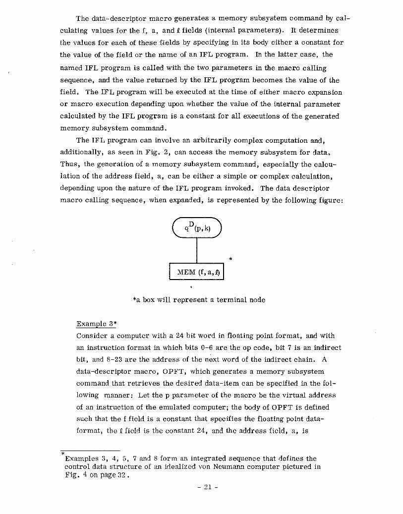
The data-descriptor macro generates a memory subsystem command by cal-
culating values for the f, a, and I! fields (internal parameters). It determines the values for each of these fields by specifying in its body either a constant for
the value of the field or the name of an IFL program. In the latter case, the
named IFL program is called with the two parameters in the macro calling
sequence, and the value returned by the IFL program becomes the value of the
field. The IFL program will be executed at the time of either macro expansion
or macro execution depending upon whether the value of the internal parameter
calculated by the IFL program is a constant for all executions of the generated
memory subsystem command.
The IFL program can involve an arbitrarily complex computation and,
additionally, as seen in Fig, 2, can access the memory subsystem for data.
Thus, the generation of a memory subsystem command, especially the calcu-
lation of the address field, a, can be either a simple or complex calculation,
depending upon the nature of the IFL program invoked. The data descriptor
macro calling sequence, when expanded, is represented by the following figure:
*a box will represent a terminal node
Example 3*
Consider a computer with a 24 bit word in floating point format, and with
an instruction format in which bits O-6 are the op code, bit 7 is an indirect
bit, and 8-23 are the address of the next word of the indirect chain. A
data-descriptor macro, OPFT, which generates a memory subsystem
command that retrieves the desired data-item can be specified in the fol- lowing manner: Let the p parameter of the macro be the virtual address
of an instruction of the emulated computer; the body of OPFT is defined such that the f field is a constant that specifies the floating point data-
format, the P field is the constant 24, and the address field, a, is
* Examples 3, 4, 5, 7 and 8 form an integrated sequence that defines the control data structure of an idealized von Neumann computer pictured in Fig. 4 on page 32.
- 21 -
calculated by an IFL program, (INDIRECT) which, using the parameter
p, generates the bit address of the last element of the indirect chain.
The expansion of the macro calling sequence OPFT (p, k) is then repre-
sented by the following figure:
L MEM (floating point, INDIRECT (p,k), 24)
The IFL program INDIRECT is not invoked at macro expansion time but
rather at macro execution time since the address field, a, of the memory
subsystem command will be recalculated for each execution of the macro
OPFT.
The instruction macro, when expanded, generates an I/O control structure
that defines the interaction between a functional unit and the memory subsystem.
The basic form of the I/O control structure generated by the instruction macro
is very similar to the basic form of the control structure generated by the
hierarchical macro; that is, a group of son nodes together with a clocking process.
The basic difference between these two types of control structures is the format
of the clocking process that is used to sequence the son nodes. The hierarchical
macro clocking process is an arbitrary process while the instruction macro
clocking process has a fixed format. The son nodes of an instruction macro
specify the data-accessing procedures which fetch (store) the input (output) data sets of the functional unit. The built-in clocking process of the instruction macro,
ICP, is activated with four internal parameters: fu, the name of a functional
unit*; &, the number of input set generator nodes (the number of output set generators are the remaining son nodes); cf, control information sent to the func-
tional unit; s, an address in the memory subsystem where the status of the functional unit at the termination of its operation is stored. The internal param-
eters fu, cf, and s can, if desired, be recalculated for each execution of the
* fu can also refer to an IFL program which simulates the action of a functional St. ‘The use of apseudo-functional unit will be discussed in V. D.
- 22 -
instruction macro 0 However, the parameter, @, can be only calculated at
macro expansion time since it relates to the form of the I/O control structure.
The instruction macro calling sequence, when expanded, is represented by the
following figure:
The clocking process ICP when executed, activates the functional unit fu with
control information,cf, and then waits for a request by the functional unit for input
or output data. When input data is requested, the calling sequence qI(pI, kl) is
activated to generate a single input value. Upon further requests for input
qI(pl, kI) is executed again until it produces no more data (e.g., it is terminated)
and then q2(p2, k2) is activated. The same process is then repeated with q2(p2, k2).
If an output is requested, qin+i(pin+i, kin+I) is activated to store a value. Upon
further requests for output, an analogous process to the input case just described
is carried out. A functional unit can also operate in the mode where it requests
all its input data simultaneously, in which case all the input generators 11’ D *Iii,
are simultaneously activated to generate inputs. At the termination of operation
of the functional unit, the status of the unit is stored starting at address s in the
memory subsystem.
Example 4
Consider the computer detailed in the previous example. An instruction
macro INSTFORMAT’(p, k) which generates a functional unit subsystem
command that emulates instructions of this computer can be defined in the
following manner. Let the p parameter of the instruction macro be the
virtual address of the instruction to be emulated, and assume that the
implicit second operand and result operand of the instruction is the accu-
mulator 0 The body of INSTFORMAT is defined such that the following
- 23 -
control structure is generated.
INSTFORMATI(p, k)
where fu is calculated by an IFL program, defined in the macro body
INSTFORMAT’, that extracts bits PO-P6 from the memory subsystem,
and ACCD(p, k) generates a fixed data-descriptor which represents the
area in the memory subsystem set aside as the accumulator.
The instruction macro can also be used to construct I/O control structures
that represent a pipeline of functional units. The pipelining of functional units
makes unnecessary the use of the memory subsystem as a temporary storage
buffer for data that passes directly from one functional unit to another. An
example of a control structure for a two level pipeline (inp- JfU11-lfuZI- out)
is the following:
2%L 0, 1 ICWu,,L,) 1 (INPU(p,,k,)) (q:(p,&))
The semantics associated with execution of this control structure is the following.
The execution of q1 activates functional unit, fuI, with input generated by INP D
*
The output of fuI is then stored by qi* But, qi is an instruction macro. In that
case, the output directed to q: is sent as an input value to fu2 after all the input
data generators of qi are exhausted. In this particular example, there are no
input generators so that output of fuI is immediately gated into fu2* Thus,
- 24 -
creating a two-level pipeline. Trees of functional units can also be created by
this same mechanism; except in this case of a tree of functional units, the control
structure is set up so that the instruction macro is requested to produce an input
instead of storing an output. The output generated by the instruction macro is
then outputted when all the output set generators of the functional unit are
exhausted. The semantics of the data-descriptor macro and the instruction macro have
been chosen so as to clearly divorce the function of data-accessing from the
computational algorithm (functional unit) D This separation then facilitates 1) the definition of I/O control structures which directly emulate different types of IML
instruction formats and 2) the incorporation of functional units into the functional
unit subsystem that have complex input and output requirements (e.g., a matrix
multiply unit, etc O).
E. Structure Building Macros
1. Sequential Control Structures
The selection macro serves the same purpose in the SBL as does the Case
statement in ALGOL, the Computed Go To statement in FORTRAN, or the data-
dependent jump instruction in machine language. The selection macro provides
a mechanism which allows the conditiona expansion of a node in the control data
structure. In essence, the selection macro defines a one-level decoding tree
which results in the generation of an arbitrary macro calling sequence. The expansion of a selection macro, q’(p, k), results in the generation of another
macro <(p,k) where the values of q,p, and k are either constants specified in the
macro body or are computed by an IFL program using p and k as parameters. The selection macro, when expanded, produces the following structure in the
process space memory:
where SEL is a built-in control process with five internal parameters that gener-
ates and then executes the macro calling sequence q&k) as its brother node. The
- 25 -
internal parameter q. is an address in the program memory, and is added to the
integer value, INC, so as to generate the address of macro i. The parameter
q. can be thought of as the base address of a vector of alternative processes
while INC is an index into the vector that determines the desired alternative.
The internal parameter q. relates to the form of the selection control structure,
and thus cannot be computed after each new execution. The internal parameter
c is control information that defines how the macro calling sequence i&E) will
be activated when qs is executed.
Example 5
Consider a computer with several different instruction formats a The
emulation of instructions of this computer could be programmed by
having a separate instruction macro INSTFORMAT;, for each instruc-
tion format J. A selection macro INSTDECODES could then be used to
select the correct instruction macro for each emulated instruction.
The iteration macro serves the same purpose in the SBL as does the
FOR-LOOP in ALGOL, the DO-LOOP in FORTRAN, or the MAPCAR function
in LISP. The iteration macro provides a mechanism for building sequential
processes. An iteration macro, qIT(p, k), defines a sequential process by
generating and executing a list of macro calling sequences:
The iteration macro defines only a sequential process because each macro calling
sequence qi(pi,ki) is completely executed before the generation of the next calling
sequence qi+I(pi+l, ki+I)’ The iteration macro, qIT, when expanded produces
the following structure in the process space memory;
- 26 -
where SCP (Sequential Clocking Process) is a built-in clocking process that
generates and then executes successive elements of the list of macro calling
sequences. The SCP, after the generation of each calling sequence qi(pi, kg,
then executes this calling sequence as its brother node. The iteration macro
may be activated by a control macro so that only a single macro calling
sequence qi(pi,k.J is executed, and then after the termination or suspension of
this calling sequence the iteration macro is suspended. Upon reactivation of the
suspended iteration macro, depending upon whether qi(pi,ki) is terminated or
suspended, respectively, either the next calling sequence qi+I(pi+I,ki+I) will be
generated and then executed or else qi(pi,k.J will be reactivated.
The clocking process SCP is activated with five internal parameters: the
first two parameters, M and V, are the addresses of IFL programs; the third
parameter, c, specifies control information; the remaining parameters po, k.
are used to construct the initial calling sequence in the list. The M program
called with parameters (pi, ki) computes qi+I, the location of a macro. The V
program, also called with parameters (pi, ki), computes (P~+~, ki+I), which are
the corresponding parameters for qi+iO The M and V internal parameters relate
to the form of the iteration control structure and thus cannot be varied from
execution to execution. The clocking process SCP terminates the generation of
calling sequences when kn+I = 0.
Example 6 Consider‘the Algol Procedure:
PROCEDURE FORLOOP (A, B,C,N);
ARRAY A [l:N], B [l:N], C [l:N];
INTEGER I; FOR I - 1 step 1 until N
DO A [I]- B [I] * C [I];
END
- 27 -
This procedure can be represented in terms of the following control data
where parlist is a pointer to the parameter list (A, B,C,N); INDEX is an
IFL program that generates the sequence of pairs (1, N) (2, N-l) . a D (N, 1);
and ARRAY is a data-descriptor macro that retrieves (stores) the ith word
of an array. It is assumed the data elements of the array are 24 bits in width. This control structure, once expanded, need not be reconstructed
for further procedure calls, only the value of parameters A, B, C, and N
need be recomputed on each execution.
The control information c is used to define how the macro calling sequence will
be activated; namely, if qi is itself an iteration macro, whether it will be activated
either for a single cycle and then suspended, or whether it will be activated for
the entire list of macro caIling sequences and then terminated. Thus, the time grain (smallest unit of work which can be controlled) of a control structure that
is constructed out of a series of successive functional decomposition of a sequen-
tial process can be set at any desired level in the decomposition.
Example 6A
Consider the iteration macro, AIT(p,k) , which when executed generates
and executes the following list of macro calling sequences BIT(p,, “I), , a .,
BIT(pn, kn) e Likewise, consider BrT(pi, ki) which when executed generates
- 28 -
and executes the following list of macro calling sequences CD(&,l$), 0 0 D,
CD(im, Em). If the iteration macro A IT is executed for a single cycle,
and the c parameter associated with SCP node of A is set for a single
cycle execute, then A IT will be suspended after the completion of each
data-descriptor macro CD(pi, l$ . Thus, in this above case, the time
grain of A IT . is the complete execution of macro C D 0 While if the c
parameter is set for execution until termination, then A IT when executed
for a single cycle will be suspended after the termination of iteration
macro BIT(pi, k$ ., Thus, in this latter case, the time grain of A IT is
the complete execution of B IT .
Another important property of the iterated macro is that generation of the
macro calling sequence qi+I(pi+I, i+l k ) may be affected by the results of executing
the macro calling sequences qI(pI, kI) . . D qi(pi, kg. The execution of a macro
may produce side effects by modifying the contents of the memory subsystem or
the control data structure which in turn may effect the execution of the M and V
programs Q This ability to alter the generation pattern of iteration macro via
side effects is crucial to defining the sequencing of machine language instructions.
Example 7
Consider an iteration macro INSTEXEC?(p, k) which generates the follow-
ing sequence: INSTDECODEs(p,, kI) , 0 o m INSTDECODEs(pi, k$, a e 0 where
pi is interpreted as the address of an instruction of an emulated computer,
and ki is the state vector of the emulated computer. The selection macro
INSTDECODES in turn generates an instructor macro INSTFORMAT:(pi, ki) ,
where J refers to the format of the instruction stored at pi0 INSTFORMAT:
when executed carries out the semantics of the instruction at location pi.
Therefore, the iterated macro can be thought of as the sequencing unit of
a computer, the selection macro as the decode unit, and the instruction
macro as the arithmetic and logic unit. This control structure in this ex-
ample can be very easily extended to include an interrupt structure. Al1
that is required is to set up a clocking process that activates INSTEXEC IT
for one cycle at a time, and then checks whether an interrupt requires
processing. In this case, the time grain is set as the execution of a single
emulated instruction.
- 29 -
The iteration macro can also be used to construct data-accessing procedures
when qi(pi, ki) is a data-descriptor macro calling sequence. The iteration macro
in this case can be considered an operand name generator and the data-descriptor
macro a value generator. An additional use of the iteration macro is the building
up of a co-routine structure since the iterated macro holds its state when sus-
pended. By combining these two uses of the iterated macro (as a data-accessing
procedure and a co-routine), a stack data-accessing structure can be constructed.
2. Nonsequential Control Structures
The hierarchical macro provides a mechanism for defining control structures
that contain more than one clocking process (path of control), l2 especially con-
trol structures that distribute control through a hierarchy of control levels. A
distributed control structure, constructed by a sequence of hierarchical macros,
can be used to define, depending upon the number of clocking processes that are simultaneously executed, either quasi-parallel 13 or parallel control structures.
In addition, many sequential control structures can also be easily defined in terms
of a distributed (quasi-parallel) control structure, e.g., a subroutine call
mechanism : the execution of the subroutine call suspends the clocking process
of the caller, and activates the clocking process of the subroutine; the return
from the subroutine then terminates the clocking process of the subroutine and
reactivates the clocking process of the caller. The block structure and procedure
calls of ALGOL and co-routines are other examples of sequential distributed
control structures. In essence, the hierarchical macro allows the structure of
a complex process to be functionally decomposed into a set of executions of less
complex processes. Thus, the hierarchical macro, in order to represent this functional decomposition, must define (1) the set of less complex processes, and
(2) the sequencing algorithm (clocking process) for this set of processes.
The hierarchical macro, qH(p, k) , when expanded, generates a Iist of macro
calling sequences:
and then expands a macro calling sequence (q+l) (p, k) D The macro (q+l) is a
clocking process that controls through the execution of control macros the initial
sequencing of the list of macro calling sequences. The list of macro calling
sequences is generated using the same mechanism, SCP(M,V,c,po,ko), employed
by the iterated macro to generate a list. Except, in this case, the generation
- 30-
pattern of the list cannot be altered through side effects since a macro calling
sequence in the list is not executed until the entire list is generated. The
control field c in SCP in the case of hierarchical macro is used to define a
default value for control information associated with the execution of each
qi(pi, k$ D The list of macro calling sequences after its generation is stored as
son nodes of the hierarchical macro in the control data structure. The expansion
of a hierarchical macro results in the generation of the foIlowing structure in
the process space memory:
r-- ! (q+W&) i (q1(P1,kl))......(9,(Pn,kn))
The macro calling sequence (q+l)(p, k) is enclosed in a dotted box to indicate
that the results of expanding the calling sequence (q+l)(p,k) is placed in the process
space memory rather than the actual calling sequence (q+l)(p,k) s Thus, if (q+l) is an iteration macro, then the expansion of qH(p, k) would result in the following
control data structure:
The execution of qH(p, k) in this above case results in the execution of the built-in _ - - -
clocking process SCP(M,V,c,pO, o l? ) which sequentially generates and executes a
list of macros calling sequences ql(pl,El) -. O $(pi, Ei) D D. O The results of
executing this list of macro calling sequences, in turn, define the initial sequencing
of ql(pl,kl) - - 0 qn(pnr kn) O The clocking process call sequence (q+l)(p, k) does
not have any characteristics which distinguish it from other processes defined by
the SBL, Thus, a clocking process can be of arbitrary complexity and only the
parts of its structure which are changed on each execution need be modified. A
- 31 -
tree of arbitrary width and depth can then be dynamically generated since the
macro qi may itself be a hierarchical macro.
Example 8
Consider the emulation of a conventional von Neumann computer organiza-
tion with an interrupt structure. The basic form of the control structure
for an emulator for this type of computer can be constructed by combining
together the control structures discussed in examples 3, 4, 5, and 7, and
then adding a hierarchical macro that specifies the interrupt structure.
Figure 4 represents this control structure, where SEQUNIT is a clocking
then adding a hierarchical macro that specifies the interrupt structure,
Figure 4 represents this control structure, where SEQUNIT is a clocking
INTHANDLE INTHANDLE
FIG. C--The control data structure for an emulator of a von Neumann computer organization with interrupt.
process that activates INSTEXEC IT for one cycle (instruction) at a time,
and then checks whether an interrupt requires servicing; if it does, then
INTHANDLER is executed, else INSTEXECrT is reactivated and the basic
sequencing cycle is repeated.
- 32 -
The hierarchical macro can also be used to construct distributed control
structures which are not conventionally represented in terms of a tree structure.
Nontree like control structures can be represented, because, as previously
discussed, the dynamic sequencing of the tree (which is defined by clocking
processes of arbitrary complexity) is separated from the generation of the tree
structure D The sequencing of sibling nodes is, therefore, not restricted to a
predefined set of built-in sequencing patterns since the clocking process is an
arbitrary program. In addition, the time grain of a process defined by a
hierarchical macro also can be arbitrary since the time gram of the clocking
process is programmable.
Example 9
Consider the parallel control structure defined by a fork-join instruction. 14
The fork-join control structure is normally represented in terms of the
directed graph in Fig. 5a. However, if the correct clocking processes are
attached to a tree of processes, then the fork-join control structure can be
represented in terms of a tree, as viewed in Fig. 5b: the clocking process
Control-l sequentially executes the process specified by macros “PARL AB”
and C. Control-Z clocking process executes processes A and B in parallel,
and is not terminated until both processes A and B are terminated.
5a
Fork A, B
AvB Join A, B
C
5b A
r-- I Control-l i (PARL AB) ( C 1
i Control-2 1 ( A I( B 1
FIG. 5--Fork-join instruction.
- 33 -
3. Tree Structured Addressing
The control macro and IFL refer to (address) processes (macro calling
sequences) in the process space memory either. through.their absolute location
in the process space memory or their relative location in the control data struc-
ture tree with respect to the address of either the control macro calling sequence
or the macro calling sequence that invokes the IFL program. In general, a node
in an arbitrary tree structure requires k parameters to specify its address
uniquely, where k is the depth of the node in the tree. However, by employing
relative addressing for node specification and restricting the part of the tree
that can be addressed from any node, the address of a process can be specified
in terms of two parameters. The restriction on accessing only part of the tree
corresponds very closely to the restriction placed on accessing variables in a
nested block structure in ALGOL and is not a serious practical limitation.
Further, this relative addressing mode, if necessary, can be overridden by using
absolute addressing node.
The relative addressing schema is a two step process, each step using one
of the parameters. The first step, using a parameter to indicate the number of
times applies the father (antecedent) relation recursively to the relative base
node. The second step, using a parameter to specify the number of the brother,
locates a particular brother of the node which results from the first step. The address schema, where (n,l) are the two parameters, can then be specified by
the following formula: (brother’ . father” *base-node). In the case of the absolute address node, the addressing schema is (brother’ .n) where the parameter N is
the absolute address of a node.
- 34 -
Example 10
Consider the following tree:
(1)
(131) qlq A A (1, 191) (LL2) (L2,l) (L%2) (1~2~3) (1,294)
Yl E (1,2,2,1) (1,2,2,2)
Ai (1,2,2,2,1) (1,2,2,2,2) (1,2,2,2,3)
D - E
then using E(1,2,2,2,2) as a relative base node
(2, -1) addresses A (1,2,1)
(22‘4 addresses B (1,2,4)
(l,O) addresses C (1,2,2,2)
(0, -1) addresses D (1,2,2,2,1) In general, if a base node address is (a,, a2, 0 0 o an) then relative address
(i, j) refers to node (al,a2, 0 D Q a(n-i-l)‘(a(n-i)+D)’
This relative address capability can be used very advantageously in the definition
of recursive distributed control structures since a clocking process does not have
to know the exact level of the tree it is controlling. Thus, the copies of a single
clocking process can be used to control different levels of the tree.
4. Synchronization, and Control and Data Linkage Among Processes
The previous sections in this chapter have described the form, the method
for constructing and the addressing structure of the control data structure. This
section will now detail how the control macro, which is the basic building block
- 35 -
of clocking processes, uses the control data structure as a syntactic framework
within which to define nonsequential control structures.
The control macro combines the control functions of process activation
(including parameter passage) and process synchronization. The control macro
performs these control functions through operations on the data stored at a node
in the process space memory. This data can be considered the state vector of
a process, where the process is defined by the control structure generated by
the macro calling sequence stored at the node. This process state vector con-
tams seven components (q,p,k,s,c,r,d) where q,p, and k is a macro calling
sequence, s is the current state of the process, c is control information associated
with the activation of the process, and r and 3 are pointers to nodes that, respec-
tively, define the immediate global control and data environment of the process.
The control information, c, specifies the time grain of the process, the conditions
for the process signalling its external clocking process, and the conditions for
rebuilding the process’ control structure; the time grain of a process can be
defined to be the execution of the process’ internal clocking process for either a
single cycle or until it is terminated; the time grain of a process defines at what
points a process’ activity can be suspended. A process can signal its external
clocking process when the process’ state is expanded, suspended, terminated,
or either suspended or terminated. The immediate global control environment
pointer, r, conventionally called a return link specifies the address of this external clocking process that will be signalled. The c component also specifies
whether a process’ control structure will be partially rebuilt after each execution
of the process, or either partially or completely rebuilt after the process is
terminated O The immediate data environment pointer, d, is used by the tree
address mechanism to locate nodes in the process space memory. The values of r and d when a node is initially generated are, respectively, the addresses of
node’s clocking process and father V However, these default options for r and d
can be overridden by the control macro so as to create a control data structure
for the passage of control which is not a tree structure.
- 36 -
Example 11
Consider the following ALGOL program, discussed in a report by Shaw 15 :
A: begin real al, O o -, an;
procedure r;
b-real rl, D oD, r m’
R: r end r; -
Al: r;
end A -
r is called at Al; after r is called recursively for the first time at R, the
control data structure has the following form:
In this example, the immediate global data environment is the same for
both instantiations of R. This example points up the distinction between
the control and data environment of a process, and the necessity for being
able to construct each of these environments independent of one another
and to override the normal tree structure discipline for representing control and data relationships among processes.
- 37 -
A node contains, in addition to process state vector, the address of the
node’s first son. The locations of a node’s siblings are implicitly defined since
sibling nodes are stored in consecutive locations in the process space memory.
The control macro, q’(p, k), when expanded, generates the following control
structure:
CM(n, Q, svt, syn)
where CM is a built-in clocking process with four internal parameters, The
first two parameters, n and I specify the relative address of a node in the contro1
data structure. The third parameter, svt, is a template for a process state
vector where for each of the component of vector there is stored in the template
either a value or null symbol. The fourth parameter, syn, is used to synchronize
the activity of the control macro with the activity of the process located at (n, 1) m The execution of the built-in clocking process CM results in the modification
of the state vector of the process located at relative address (n, 1) in the process
space memory. This process’ state vector is modified by replacing the value of
each of its components by the corresponding svt component whenever this corre- sponding svt component is not null. Thus, only the components of the state vector
of the activated process which vary from execution to execution of the process
need be recalculated and then replaced by the control macro. The static compo-
nents of a process state vector (the fixed control and data linkages of a process) are defined either by default options when the process’ state vector is initially
generated or by the control macro which initially expands the macro calling
sequence that defines control structure of the process. Thereafter, the control
macro that activates the process has a template state vector whose components are null whenever the corresponding components of the process’ state vector are
static D At the same time as the modification of the process’ state vector is
completed, the s component of the state vector of the CM clocking process is
modified, depending upon the syn parameter, to be either the suspended or the
terminated state. Through this mechanism of simultaneous modifying of two
state vectors, the activity of one process can be synchronized with activity of
another process I
- 38 -
Example 12
Consider two processes A and B, where process A calls process B as
a subroutine. Process A performs the subroutine call by executing and
then waiting for termination of a CM clocking process. In turn, the
CM clocking process activates the process B and modifies B’s state
vector so that process B will signal a return when it is terminated, and
this return will be to the CM clocking process. At the same time, the
syn parameter of CM is set up so that after process B’s state vector is
modified the CM clocking process is suspended. When process B is
terminated, CM will then be re-awoken and will go to the terminated
state. This action in turn will allow process A to continue processing
since process A has been waiting on the completion of the CM clocking
process, If process A was not synchronized with the activity of process
B then e parameter of CM would be set up so that after process B is
activated the CM process is terminated. Thus, process A after process
B is activated will immediately continue processing. Process A while
waiting for CM process to terminate is not suspended because the action
of suspending process A may be significant to A’s external clocking
process since the suspending of A means that process A has completed
a time grain, Thus, this implementation of subroutine call permits A’s
external clocking process to view A as executing while process B is
executing, but at the same time A’s internal clocking process is waiting
on B’s completion,
The CM clocking process can only activate a process for execution (e.g.,
change the s component of the process’ state vector to executing) when the process’
current state is unexpanded, expanded, suspended or terminated. In the case
that CM clocking process attempts to execute an already executing process, the CM clocking process either is suspended or goes into a busy wait until the process
to be executed is no longer executing. The time grain of the node that generates
the CM determines which one of these options is taken: if the time grain is a
single cycle the CM is suspended, otherwise it busy waits. Thus, if two processes
simultaneously issue CM’s which activate the same node (shared process), only one
CM will be allowed to execute the shared process. The other CM will then either
wait till the shared process is completed, or possibly at some later time try to
- 39 -
execute the shared process. This paradigm for sequentializing the execution of
a shared process can then be used as basis for constructing synchronizing prim-
itives for cooperating processes.
Example 14
Consider the implementation of Dykstra’s P and V semaphores in terms of
the CM clocking process D Let PV be a shared process where the p compo-
nent of its state vector is the name of semaphore variable to be operated
on, the k component of its state vector indicates whether a P or V operation
is to be performed, and the r component is the address of the process that activated PV. A process Li performs a P or V semaphore operation by
generating a CM clocking process whose time grain is termination, G
parameter in the case of P operation specifies suspended while for a V
operation specifies terminated, (n, 1) parameters specify the relativeaddress
of the PV process, and the ss contains the correct calling sequence for
either a P or V operation. The PV process when executed by CM for a P
operation checks whether the semaphore variable specified in the calling
sequence can be decremented, if it can, then the operation is completed
and the PV process is suspended. This suspension of PV results in ter-
mination of CM which then permits process Li to continue. In the case that semaphore can not be decremented, the PV process modifies its own state
vector component so that it does not return to CM when it is suspended. It then extracts the address of the CM process from its state vector, places
this address in queue associated with the semaphore name, and suspends
itself. Thus, the CM clocking process still remains in the suspended
state, and therefore process Li can not continue. The PV process when
executed for V operation increments the semaphore variable, and then
checks whether there is a queued CM process on that semaphore variable that can now be executed. If there is, this CM process address is stored
in the r component of PV state vector, and PV process then suspends itself
which results in the queued CM process to be re-awoken. The CM
clocking process that executed the PV process for a V operation termin-
ates immediately after the PV process state vector has been modified, and thus Li can continue processing while V operation is being done. If the PV process is busy, when CM attempts to execute it, then CM goes
- 40 -
into a busy wait, however, this busy wait is not on a semaphore variable
but only on the process which updates the semaphore.
The CMcan also be used to create a new copy of a process (node) instead of
calling a shared process, This creation of new node occurs when the (n, 1)
parameter are (0,O) 0 The new node is the root node of a separate tree, and only
the CM clocking process can access this tree. It may be also advisable, for
efficiency reasons, for a CM clocking process to be able to simultaneously acti-
vate all the sibling nodes at level in tree, and then be able to wait for all of them
to signal a return.
- 41-
V. INTEGER FUNCTION LANGUAGE (IFL)
The IFL is a highly specialized micro-code language designed specially for
the task of address arithmetic computations. The output of the address arithmetic
computations performed by the IFL are then used in the expansion and execution
of SBL macros. The format of IFL instructions and SBL macros are very similar;
each is called with two parameters, and each has an expansion and execution phase,
In fact, the execution of SBL* and IFL statements can be intermixed, and the same
syntax will be used to define an IFL instruction calling sequence as is used to de-
fine an SBL macro calling sequence (e.g., qF(p,k), (lO)(p,5), etc., where F is
for the convenience of the reader to differentiate an IFL calling sequence). The
basic difference in a conceptual sense between the IFL and SBL is that the execu-
tion of an IFL instruction results in the execution of a function which returns an
integer value whereas the execution of SBL macros results in the execution of a
process D Thus, the IFL instruction can be considered a “functional macro”.
The basic reason for not defining address arithmetic algorithms in terms of an SBL
control structure stems from the use of a different control structure for address
arithmetic functions than that for processes. In particular, the control structure
for defining address arithmetic functions can be much less complex and variable
than that required for processes. Thus, the sequencing schema for IFL instruc-
tions is built-m rather than explicitly defined, as in the case of the sequencing
for SBL macros. Address arithmetic algorithms can, therefore, be executed
without the overhead of a variable control structure used for defining a process
control structure.
Before formally defining the syntax and semantics of the IFL, it is worth-
while to note the following characteristics of the IFL which differentiate it from
conventional micro-code instruction sets:
1. Parallelism: the IFL can execute, ‘wherever appropriate, parallel
(concurrent) activity in an address arithmetic computation.
2. Modularity: complex IFL program can be easily constructed out of calls to other IFL programs (the concept of a recursive function is
an integral part of the control structure of the IFL); each IFL instruc-
tion is called with two parameters and then returns an integer value.
* The execution of an SBL macro in the context of an IFL program results in the expansion and then complete execution of the macro. After its termination, the next statement in the program memory is executed, and the control data structure in process space memory resulting from its execution is garbage collected.
- 42 -
3. Reentrancy: the IFL interpreter does not have a fixed set of registers
but, instead, registers are dynamically created through the passage
of parameters D
4. Simplicity: the syntax (format) and semantics of an IFL instruction
are uniform (regular) and simple.
A. Format and Sequencing of IFL Instructions
The format of an IFL instruction qF, which is stored in a word in the pro-
gram memory, consists of five identically formatted fields, f q, Aq, Bq, KS, Q - q
The format of a field consists of an m bit Merger*, c, plus a 2-bit descriptor
field, d, that defines the method for calculating the value associated with the
field; a field is represented by the following notation: (d, c) s The value associated
with a field is calculated, depending upon d, in one of the four following ways:
1. c;
2. p+c;
3. k+c ;
4. ts+qF tp,k) 0 where p and k are the parameters used to call an IFL instruction q:qF(p, k) .
These three parameters, q, p and k, of an IFL instruction calling sequence, can
be considered in terms of a conventional micro-computer organization as the
current values, respectively, of the program counter, accumulator, and index
register D
The expansion phase of the instruction calling sequence q(p, k) is the parallel
evaluation of the five fields, f , A , B ,K ,Q q q q q q’
based on the above rules. These
five fields have the following semantics associated with their values: fq ( the
name of dyadic integer function which is the op-code of the IFL instruction 9); Aq and Bq (parameters for the function fq), Kq (a counter used to define termina-
tion of sequencing), and Qq (an increment used to indicate the relative address
with respect to q of the next IFL instruction) O
* The maximum size of c which is dependent on m does not have to have an rela- tionship to the maximum size of addressing space in the program memory or the memory subsystem. The choice of a value for m will be based on consider- ations of code density and speed of execution.
- 43 -
Example 14 Consider the IFL instruction FACT which has the following five field
formats : (1, ‘K*‘t), (2,0), (3,0), (3,-l), (1,O). The expansion phase of
FACT(p, k) then results in the five fields having the following values:
fFACT’*tmU1tiply), AFACT?, BFACT=k, KFACTK, -1, and QFAcT=O.
These five values generated by the expansion phase are then used in the
execution phase of q(p, k) to define the execution semantics and sequencing of
IFL instructions in the following manner:
qb 9 F.- if k=O then p else (q+QdF (fq(Aq, Bq), Kq)
This paradigm for execution of IFL instructions results in the generation of a
sequence of triplets: (qO,po,kO) (ql,pISkl) D 00 (qn,pn,kn) (qn+l,Pn+l,O), where qo=q, po=p, ko=k, and for i 2 0, pi+1 = f (A ,B ), ki+l=Kq, and
9i 9i 9i qi+1’9i+Qq o The value P,+~
i is then returned to the process that ca;ed qo.
Example 15
Consider the IFL instruction, FACT, discussed in Example 14. The exe-
cution of the calling sequence FACT(p, k) then results in the following cal- culation:
FACT(p, k) c if k=O then p else (FACT+O) (p*k, k-l)
If p and k have the following initial values of, respectively, 1 and N, then
FACT( 1, N) when executed calculates N! in the following iterative manner:
FACT(l, N)- if N=O then 1 else (FACT+O) (N*l, N-l) = FACT(N, N-l)
FACT(N!, i)+ if i=O then N!/i! else FACT(N!/(i-l)!, i-l) D . D
FACT(N!/O:, O)=N!
This calculation generates a sequence of triplets: (FACT, 1, N)
(FACT,N,N-1) m*D (FACT,N!/il,i) DoS (FACT,N!,O).
- 44 -
The sequencing part of the execution paradigm for IFL instructions is very
general, and allows as special cases, iterative, straight-line, and conditional
sequencing of IFL instructions, plus a value return mechanism.
1. iterative sequencing, as seen in example 15, occurs when Qqs 0,
then q(p,k), if k=O then p else q(pI, kI) D
2. straight line sequencing occurs when Qq= 1, then q(p, k), if k=O then
p else (q+l)(pl, kl); in addition, if k is always not zero when q is called,
then q@,k)+ (q+l)(plskl) D 3. conditional sequencing occurs when the field Qq is an expression rather
than a constant.
4. a value return occurs when Kq=O, then q(p, k).- if k=O then p else (q+Qq) (p,, 0), but (q+Qq) (p,, 0) = PI, and thus q(p, k)- if k=O then p else PI;
in addition, if k is always not zero when q is called, then q(p, k)-pIO
In addition, parallel and recursive sequencing of IFL instructions may be
programmed 0 Parallel and recursive sequences of IFL instructions arise because
the values associated with five fields can be calculated in parallel and may result
(when the descriptor, d, of a field is equal to 4) in the calling of an other IFL
instruction.
Example 16
Consider the following two IFL instructions, X and Y, which have the
following field values:
X If,=*, Ax=Y(p, k), Bx=k, Kx=O, Q,=O)
Y ={fy=+, Ay=p, By=O, Ky=k-1, Q,=-11
where Y = (X+1)
The execution of the calling sequence X(p, k) then results in the following
calculation:
Wp,k)+ if k=O then p else (X+0) (Y(p, k) *k, 0) which is equivalent to
Wp,k), if k=O then p else Y(p, k) *k, where
Y(p,k)+ if k=O then p else (Y-l)(p,k-l), however
X(p, k) only calls Y(p, k) when k#O, and also (Y-l) =X.
Thus Y(p, k) c X(p,k-1); and then
Xbk)-- if k=O then p else X(p, k-l) *k
If p and k are initially, respectively, 1 and N, then X( 1, NJ
calculates Ni in a recursive manner since:
X(1, N)+- if N=O then 1 else X(l,N-l)*N.
- 45 -
The SBL and IFL interact through the generation by the SBL of an IFL
calling sequence, qF(p, k) D The result of executing this calling sequence is the
return of either a single value P~+~, or each pair in the sequence (p,,kI) Q D D
(p,, kn) . This latter type of return is used to define the execution of the iteration
macro and results in a co-routine type interaction between the SBL and IFL since
the IFL program is suspended after each pair (pi, ki) is generated.
Example 17
Consider the sequence of pairs (l,N)(2, N-l) 0 o D (I, N-1+1) D 0. (N, 1) used
in defining the iteration macro that represents the ALGOL statement for
I..- 1 step 1 until N do A [I J .- B[ I J * C[ I J s This sequence of pairs can be
generated by the IFL instruction, INDEX, which has the following field values, f =r,+r,
INDEX 9 AINDEX~, BINDEX=L KINDEX*-L and QmDEx=O’ The IFL instruction calling sequence INDEX(0, N+l) when executed then
generates the following sequence of pairs: (1, N) *. o (i, N+l-i), (i+l, N-i) 0 . m
(N, 1) in the following manner:
INDEX(i, N+l-i)-if (N+l-i)=O then i else INDEX(i+l, N-i)
In order to clarify the discussion of IFL programs presented in later sections, the assembler notation specified in Table 1 will be used for describing IFL instruc-
tions and programs. This symbolic notation for IFL instructions can be mapped
directly (one-one) into actual IFL instructions. The major purpose of the assem-
bler notation is to represent the special IFL sequencing cases, previously
described, with a symbolic notation that indicates each of the special cases.
Table 2 indicates these relationships between assembler syntax and special cases of IF L sequencing D
Example 17A
Consider the IFL instructions FACT,X,Y discussed previously. These IFL instructions can be symbolic represented as follows:
The types of functions which fq field can represent fall into three classes:
interger arithmetic operations, conditional and selection operations, and memory
access operations. The interger arithmetic operations contain the conventional
arithmetic and logical operations, concatenation, and shifting. Therefore, if
fq=+ then fq(Aq,Bq) equals A +B 0 4 q
The concatenation and shifting operators
allows building a larger size constant from two smaller size constants or the
combining of disjoint memory fields. The conditional operations test a condition
between the two operands and, depending upon the satisfaction of the condition,
produces either 0 or 1:
if fq = “>” then fq(Aq, Bq) = if Aq > Bq then 1 else 0
The selection operation, IA and IB, which are, respectively defined by field value
for fq of 1 or 0 have the following definition:
IA(Aq, Bq) = Aq and IB(Aq, Bq) = $
The conditional and selection operators can then be combined to construct
if-then-else arithmetic statements.
Example 18
Consider the function X(I) which has the following definition: if I> 5 then
I else 5. The function X can be programmed in terms of two IFL instruc-
tions C and D, where
C : PUP, 5) ; D: p>5;
Let C be called with parameter (I, 1) then C(1, 1) .- [ D(1, l)] (I, 5)) and
D(L 1) - if I>5 then 1 else 0.
Since [ 11 (I, 5)~ IA(I,5) = I and [O] (1,5) = IB(I,5) = 5 then
C(L 1) - if 115 then I else 5.
There are two types of memory access operators: one to access the memory
subsystem and the other to access the process space memory. The memory
subsystem operator M(Aq, Bq) extracts from the memory subsystem starting at
bit Aq a string of length B 0 This string of bits is interpreted as an integer
value D The process space’memory operations P1(Aq, Bq), P2(Aq, Bq) . . e PWq, Bq),
- 48 -
retrieve, respectively, one of the six components of the process state vector B located at relative address (As, q ) in the process space memory.
Example 19
Consider the addressing structure of the PDP-6. Each PDP-6 word is 36 bits long and is divided into three fields for addressing: an indirect
field, I, (Bit 13), an index field, B, (Bits 14-17), and an address field,
A, (Bits 18-35). The index registers in the PDP-6 are the first 16 words
in memory. The addressing structure of PDP-6 is indirect addressing
with indexing at each level of the (arbitrarily long) indirect chain. The
first problem is how to represent the 36-bit wide word memory in the
memory subsystem. Let us lay out PDP-6 memory starting at bit 0
in the memory subsystem so that word K of the PDP-6 begins at address
M[ K*36] and ends at M[ K*36+35] D The following IFL program deter-
mines the address of the last word in the indirect chain giving the address of the first word of the chain:
PDGADD: if k=O then p else p:=p*36, go to [k] (CHAIN, EXTRACT-A) ;
CHAIN:p:= [EXTRACT-A] + [EXTRACT-B],
k:= [EXTRACT-I], go to PDGADD;
EXTRACT-A: M(ptl8, 18) ;
EXTRACT-B: p:=M(ptl4, 4)) k:=2,
go to PDGADD;
Comments
Converts virtual address
to physical address and
then gets value associated
with physical address
Basic sequencing of
indirect addressing
Extracts address field
Extracts index field and
then calls procedure to
get value of index
EXTRACT-I: M(p+13, 1) ; Extracts indirect field
The IFL program PDGADD is called with parameters (a,, 1) where al, iS the
address of the first word of the chain.
Large size address constants can be generated by IFL instructions either
through the concatenation of smaller size address constants or by storing
- 49
beforehand the constant in the memory subsystem and then, when the constant
is required, extracting it from the memory subsystem. Though the above is a
conceptually adequate solution, for reasons of execution efficiency and code
density, an additional instruction format has been added to the IFL to handle
large size address constants. This added type of instruction format, L, has the
following format:
word q L I
d 42 I 2 5M+8
where d has the same semantics as it has in the basic instruction format of IFL
instruction, and Lc is an address constant which fills the rest of the program
memory word. Thus, the value of qL(p,k) depending upon d is computed in one
of the four possible ways: 6, p+fc, k+lc, or (q+a,) (p, k) O
C. Side Effects in IFL
The IFL, as so far presented, is very similar in two significant ways to
“pure LISP”; each creates temporary storage solely through parameter passages
and each has no side effects other than the return of a value. These character-
istics of the IFL, though theoretically interesting since they guarantee the deter-
mininacy of parallel IFL computations, severely limited the ability of this micro-
computer to emulate existing computers I) In particular, the programming of
address arithmetic computations for emulator may involve more than just the
return of a value; e.g., an effective address calculation may also involve checking
for an address alignment error, and, if necessary, then updating the state vector
of the emulated computer to indicate the addressing error. Thus, the IFL contains
provisions for the programming of side effects.
The IFL contains memory operations which can modify the contents of either
the memory subsystem or the process space memory. These memory operations
SM, SPl, 00. SP6, are the store counterparts, respectively, of the memory
access operation M, Pl, . DO P6. The memory store operation stores the p
parameter of an IFL calling sequence in the designated place in the memory sub-
system or process space memory. In addition, an IFL can be executed in a call
by value or call by name mode. In the call by value case, the values of fq(Aq, Bq) and Kq are stored in, respectively, new temporary storage locations p1 and kl,
- 50 -
while in the call by name case, * the values of the parameters p and k are,
respectively, replaced by fq(Aq,Bq) and K 0 The call by name case is used q
when the p and k parameters are pointers either to fields in the memory sub-
system or to p or k components in the process space memory. Thus, side
effects in IFL can be programmed in two ways: directly through memory store
operations or indirectly through the call by name mode.
The call by name mode is distinguished from the call by value mode through
two control bits attached to the IFL instruction format previously discussed.
There are also three other control bits, attached to each IFL instruction. These
three other control bits are used to sequence the evaluations of the five fields in
the IFL instruction and, thus, override the normal parallel evaluation. ? These
field sequence control bits allow the programmer to specify the order of evalua-
tion of fields so as to avoid indeterminancy in IFL computations when one or
more of field evaluations result in side effects. In addition the IFL, contains
three other memory operations, PM, PP2, and PP3, whose execution results in
the generation of a pointer to, respectively, a field in the memory subsystem or
to a p or to a k component in the process space memory.
D. Pseudo-Functional Units
An IFL program can be used to simulate the actions of a functional unit in
the functional unit subsystem. This use of an IFL program occurs when the
value of the fu parameter of an instruction macro is greater than the number of
functional units in the functional unit subsystem. In this case, the fu parameter is interpreted as the starting address in the program memory of an IFL program. The IFL program activated by the instruction macro then interacts with the
input data and output data generators of the instruction macro through the following
operations: FI, FIF, FIA, FIL, FO, FOF, FOA, FOL, FC, FS and FIN. The
FI operation activates an input generator of the instruction macro and the bit
The notation used in the assembler to distinguish a call by name from that of a call by value is the following: p ..- <PEXP> is a call by name while p:=@EXP> is a call by value.
t The eight possible strategies for evaluation of the five fields have not yet been fixed.
- 51-
string produced by the input generator is the output of the FI operation. The
FIF, FIA, and FIL operations retrieve from the input generator, respectively,
the format, address, and length of the next input data item to be generated. The
FO, FOF, FOA, and FOL operations activate an output generator and are the
output analogs of FI, FIF, FIA and FIL operations. The FC and FS operations
retrieve, respectively, the c and s parameters of the instruction macro. The - FIN operations is used to determine whether there is any more input data to be
processed, These operations in conjunction with the other IFL operations
previously discussed allow IFL programs to simulate an arbitrarily complex
functional unit.
- 52 -
VI. FORMAT OF SBL MACROS
An SBL program, like an IFL program, is stored in the program memory.
The format of a word in the program memory that defines an SBL macro body is
identical to the format of a word that defines an IFL instruction. Further, the
definition of a macro body, stored at address q, is specified in terms of the
values of the fields fq, Aq, Bq, Kq, and Q q0 These fields are computed for an
SBL macro definition in the same manner as they are computed for an IFL in-
struction, where the two parameters p and k that are used in computing the values
of the five fields are derived from the macro-calling sequence q(p, k) D Thus, the
only difference between the definition of an SBL macro body is the definitional
semantics associated with the values of the five fields. The different types of
macro bodies are specified in terms of a fixed set of definitional templates
(skeletons) D The values of the five fields are then used in the expansion of a
template (to fill in the blank spaces in a skeleton) where the usage of the five
fields is fixed according to the particular template being expanded. This method
for specifying the body of a macro is simple and uniform but at the same time
very powerful since the value of each of the five fields can be the result of an
The possible formats of a word q in the program memory are the following:
t q
d q
PC q
where tq specifies either the type of (template for) the macro body or the type of
IFL instruction stored at word q, and sq.is control information used in the evalua-
tion of the five fields. The type field, t q’
is 3 bits long and specifies either one
of the six possible macro bodies or one of two possible IFL instruction types.
The control field, sq, is five bits long, and in the case of an IFL instruction s q
,
specifies whether the instruction is called by name or by value and the order of
evaluation of the five fields, while in the case of an SBL macro sq specifies
whether each of five fields will be evaluated at the time of either macro expansion
or macro execution.
- 53 -
A. Data-Descriptor Macro D The data-descriptor macro, q , when expanded, results in the generation
of a terminal node MEM(f, a, n) , where f specifies the format of a data item, a - - its address, and P its length.. The values of these three parameters are computed,
based on the values of the five fields stored at location q, in the following manner:
a = fq(Aq, Bq)
l=K q
f =Qq
These three parameter values are computed at either macro expansion or macro
execution time depending upon the value of s 0 Base relative addressing can be
programmed by setting fq= ‘+‘, Aq the value’of a base register, and Bq the
address displacement relative to the base: a=A +B D 4 q
The following symbolic notation will be used to represent the data-descriptor
macro body:
<DATA-DESCRIPTOR>:=<STATEMENT-LABEL>: D MEM(<F>, <A>, <L>)
<F> := <EXP-FIELD>
<A> := <PEXP>
<L> := <EXP-FIELD>
The underlining of a parameter of MEM indicates the parameter is computed at
macro execution time rather than at the time of macro expansion. This convention
of underlining will be used for all symbolic representation of SBL macro bodies.
Example 20
Consider the data-descriptor macro, OPFT, discussed in example 3 on
page 21. The body of the macro OPFT can be specified in the following manner :
OPFTD: MEM( 1, [INDIRECT] *24, 24) INDIRECTF: if k=O then p else p:=p*24;
p:=M(p+7,16), k:= fl-BITJ, go to INDIRECT;
I-BITF : M(p+6,1) ;
The 24 bit length words of the emulated computer are laid out in consecu-
tive bit locations starting at 0 in the memory subsystem, The macro
- 54 -
OPFT is invoked with a calling sequence whose first parameter, p, is
the virtual address of the first word of the indirect chain. IFL program
INDIRECT, invoked with the same calling sequence parameters as
OPFT, computes the virtual address of the last element of the indirect
chain. Thus, the execution of OPFT(p,k) results in the execution of the
memory subsystem command MEM(f, a,4 where
f = 1, specifying floating point format;
a = INDIRECT@, k) *24, the absolute address of the last word
of the indirect chain; L = 24, the length of data word.
B, Selection Macro
The selection macro, qs, when expanded, results in the generation of a
terminal node SEL(qo, INC, c,$,@ D This terminal node, when executed, gener-
ates and then executes the macro calling sequence q(p,@, where i is equal to
q,,+INC, and c indicates the type of activation. The value of the five parameters
of SEL are computed based on the value of the five fields stored at location q in
the following manner.
The following symbolic notation will be used to represent the selection macro
body : /
<SELECTION>:=<STATEMENT-LABEL> ’ : SEL (<QO>, <INC>, <C >, <P>, <li>)
<QO>:=<STATEMENT-LABEL>
<INC>:=<EXP-FIELD>
<C z:=<EXP-FIELD>
<P>:=<EXP-FIELD>
<li>:=<EXP-FIELD>
- 55
Example 21 Consider the selection macro, INSTDECODE, discussed in example 5
on page 26, and suppose that the computer to be emulated has a 24 bit
length word where the first 2 bits of the word specify one of four pos-
sible instruction formats. The body of the macro INSTDECODE can be
specified in the following manner:
INSTDECODES: SEL (INSTFORMAT, [ DEC], 1, e, 5);
DECF: p:=p*24; M(p, 2) ;
where the macro INSTDECODE is invoked with a calling sequence whose
first parameter, p, is the virtual address of the instruction to be emu-
lated. The IFL program DEC, when executed, returns the value of the
first two bits of the instruction word. This value is then used to choose
one of four possible macros: INSTFORMAT, (INSTFORMAT+l),
(INSTFORMAT+2) or (INSTFORMAT+S). This macro is then executed
with the same parameters as used to call INSTDECODE:
6 = INSTFORMAT + DEC(p,k)
P’P i;=k
C. Iteration Macro IT The iteration macro, q , when expanded, results in the generation of a
terminal node SCP(M,V,c,po,k6). The SCP node, when executed, sequentially
generates and executes a list of macro calling sequences: qI(pI,kI), 0 D o
q,(p,, kn) a This list is generated by invoking the IFL program, V, with the
initial parameters p. and kg; V(p,, k6), executed like a co-routine as previously
described on page , generates a sequence of pairs (pl,kl) (p2,k2) *. D
(pn,kn) (P,I, 6). The first n pairs are used to define the parameters pairs in
the list of macro calling sequence. The corresponding macro qi associated with
each pair (pi, ki) is computed in the following manner:
qi = q + M(Pi-l’ki-I)
Ifthe sq bit associated with M parameter is set to evaluation at the time of macro expan-
sion rather than macro execution, then M is a constant and thus qi=q+M is a constant.
The c parameter of SCP defines whether amacro calling sequence qi(pi, k$ will be eval-
uated for a single cycle or to completion, and in the case that qi is a constant whether
the macro qi will be reexpanded for each cycle of the interation macro, reexpanded only
for each sequence of parameters (pI,kI) . 0. (p,, kn) , or never reexpanded.
- 56 -
The following symbolic notation will be used to represent the iteration macro
This paper is a preliminary investigation of the organization of a parallel
micro-computer designed to emulate a wide variety of sequential and parallel
computers. This micro-computer allows tailoring of the control structure of
an emulator so that it directly emulates (mirrors) the control structure of the computer to be emulated. An emulated control structure is implemented through
a tree type data structure which is dynamically generated and manipulated by
six primitive (built-in) operators. This data structure for control is used as a
syntactic framework within which particular implementations of control concepts,
such as iteration, recursion, co-routines, parallelism, interrupts, etc., can be
easily expressed. The major features of the control data structure and the
primitive operators are: 1) once the fixed control and data linkages among
processes have been defined, they need not be rebuilt on subsequent executions
of the control structure; 2) micro-programs may be written so that they execute
independently of the number of physical processors present and still take advan-
tage of available processors; 3) control structures for I/O processes, data-
accessing processes, and computational processes are expressed in a single
uniform framework. This method of emulating control structures is in sharp
contrast with the usual method of micro-programming control structures which
handles control instructions in the same manner as other types of instructions, e.g. , subroutines of micro-instructions, and provides a unifying method for efficient emulation of a wide variety of sequential and parallel computers.
Future research on this micro-computer organization will attempt to develop
more rigorous arguments for the merits of this proposed method for emulating control structures. In particular, a simulator for this micro-computer orgam-
zation and emulators for complex sequential and parallel IML’s will be programmed.
These emulators will then be run on the simulator to gather performance statistics. In addition, it is planned to develop a higher level language, which can be easily
compiled into SBL and IFL statements, for representing control structures of
machines D
There are two other research areas which will be investigated. The first
research area involves the addition to the SBL of primitive operators (macros)
which control access to nodes in the process space memory, fields in the memory
subsystem, and functional units in the functional unit subsystem. Thus, it is
- 61 -
proposed to integrate the concept of protection (capabilities, access path, etc.)
into the definition of the control structure of a process which is where the definition
of protection naturally belongs. In the preliminary investigation of this idea, it
appears that the concepts of protection discussed by Dennis and Van Horn, 17
Lampson, 18 etc. can be easily specified, with the addition of two or three primi-
tives to SBL, in the framework of the proposed data structure for control. Thus,
emulators for operating systems IML’s will be more easily implemented, and it
will be possible to protect a micro-code from interference by other micro-
programs. The second research area to be investigated involves applying the concept
of control structure definition language to the organization of a computer rather
than just a micro-computer. The investigation of this research area has been
prompted by the work of Mitchell 19 on the organization of an interpreter for LC2
language.
- 62 -
REFERENCES
1. Burroughs Corporation [1963]. The Operational Characteristics of the
Processors for the Burroughs B5000. Burroughs Corporation, Detroit,
Michigan.
2. Illiac-IV System Study Final Report [ 19661. Burroughs Corporation,
University of Illinois No. 09852-B.
3. Abrams, P. S. [1970]. An APL Machine. Report No. SLAC-114, Stanford
Linear Accelerator Center, Stanford University, Stanford, California.
4. Melbourne, A. J. and Pugmire, J. M. [ 19651. A Small Computer for the
Direct Processing of FORTRAN Statements. The Computer Journal,
Vol. 8 (April).
5. “System/360 Model 40,204O processing unit. ” [1966J. IBM Field Engineering
Diagrams Manual, Document No. 0223-2842.
6. cook, R. W, and Flynn M. J. [1970]. System Design of a Dynamic Micro-
processor. IEEE Transactions on Computers, Vol. C-19, No. 3.
7. Lesser, V, R. [1968]. A Multi-Level Computer Organization Designed
to Separate Data-Accessing from the Computation. Tech. Rep. CS90,
Computer Science Department, Stanford University.
8. Lass, S. [1968]. A Fourth Generation Computer Organization. AFIPS Con-
ference Proceedings, Vol. 32.
9. Horning, J. J. and Randell, B. [1969]. Structuring Complex Processes.
Report RC-2459, IBM Watson Research Center, Yorktown Heights, New York.
10. Fisher, D. A. [19’70]. Control Structures for Programming Languages,