Linear Eigenvalue Problems Non-Linear Eigenvalue Problems Additional Features SLEPc Current Achievements and Plans for the Future Jose E. Roman D. Sistemes Inform` atics i Computaci´ o Universitat Polit` ecnica de Val` encia, Spain Celebrating 20 years of PETSc, Argonne – June, 2015 1/36
Transcript
Linear Eigenvalue ProblemsNon-Linear Eigenvalue Problems
Additional Features
SLEPcCurrent Achievements and Plans for the Future
Jose E. Roman
D. Sistemes Informatics i ComputacioUniversitat Politecnica de Valencia, Spain
Celebrating 20 years of PETSc, Argonne – June, 2015
1/36
Linear Eigenvalue ProblemsNon-Linear Eigenvalue Problems
Additional Features
SLEPc: Scalable Library for Eigenvalue Problem Computations
A general library for solving large-scale sparse eigenproblems onparallel computers
I Linear eigenproblems (standard or generalized, real orcomplex, Hermitian or non-Hermitian)
I Also support for SVD, PEP, NEP and more
Ax = λx Ax = λBx Avi = σiui T (λ)x = 0
Authors: J. E. Roman, C. Campos, E. Romero, A. Tomas
Linear Eigenvalue ProblemsNon-Linear Eigenvalue Problems
Additional Features
EPS: Eigenvalue Problem Solver
Compute a few eigenpairs (x, λ) of
Standard Eigenproblem
Ax = λx
Generalized Eigenproblem
Ax = λBx
where A,B can be real or complex, symmetric (Hermitian) or not
User can specify:
I Number of eigenpairs (nev), subspace dimension (ncv)
I Tolerance, maximum number of iterations
I The solver
I Selected part of spectrum
I Advanced: extraction type, initial guess, constraints, balancing
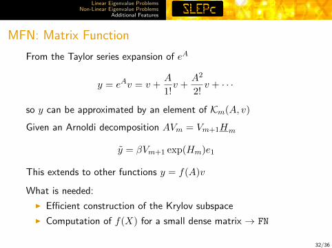
9/36
Linear Eigenvalue ProblemsNon-Linear Eigenvalue Problems
Additional Features
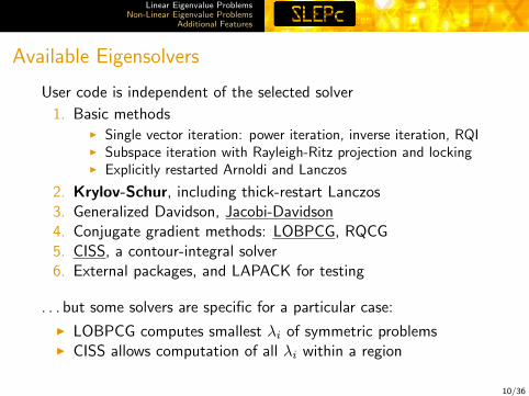
Available Eigensolvers
User code is independent of the selected solver
1. Basic methodsI Single vector iteration: power iteration, inverse iteration, RQII Subspace iteration with Rayleigh-Ritz projection and lockingI Explicitly restarted Arnoldi and Lanczos
2. Krylov-Schur, including thick-restart Lanczos3. Generalized Davidson, Jacobi-Davidson4. Conjugate gradient methods: LOBPCG, RQCG5. CISS, a contour-integral solver6. External packages, and LAPACK for testing
. . . but some solvers are specific for a particular case:
I LOBPCG computes smallest λi of symmetric problemsI CISS allows computation of all λi within a region
10/36
Linear Eigenvalue ProblemsNon-Linear Eigenvalue Problems
Additional Features
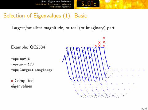
Selection of Eigenvalues (1): Basic
Largest/smallest magnitude, or real (or imaginary) part
Example: QC2534
-eps nev 6
-eps ncv 128
-eps largest imaginary
Computedeigenvalues
11/36
Linear Eigenvalue ProblemsNon-Linear Eigenvalue Problems
Additional Features
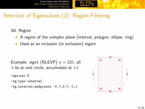
Selection of Eigenvalues (2): Region Filtering
RG: Region
I A region of the complex plane (interval, polygon, ellipse, ring)
I Used as an inclusion (or exclusion) region
Example: sign1 (NLEVP) n = 225, allλ lie at unit circle, accumulate at ±1
-eps nev 6
-rg type interval
-rg interval endpoints -0.7,0.7,-1,1
12/36
Linear Eigenvalue ProblemsNon-Linear Eigenvalue Problems
Additional Features
Selection of Eigenvalues (3): Closest to Target
Shift-and-invert is used to compute interior eigenvalues
Ax = λBx =⇒ (A− σB)−1Bx = θx
I Trivial mapping of eigenvalues: θ = (λ− σ)−1
I Eigenvectors are not modified
I Very fast convergence close to σ
Things to consider:
I Implicit inverse (A− σB)−1 via linear solves
I Direct linear solver for robustness
I Less effective for eigenvalues far away from σ
13/36
Linear Eigenvalue ProblemsNon-Linear Eigenvalue Problems
Additional Features
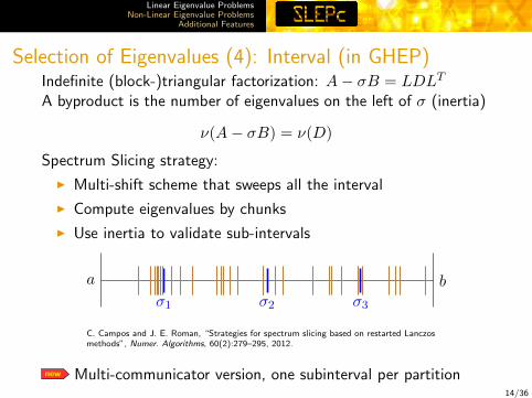
Selection of Eigenvalues (4): Interval (in GHEP)Indefinite (block-)triangular factorization: A− σB = LDLT
A byproduct is the number of eigenvalues on the left of σ (inertia)
ν(A− σB) = ν(D)
Spectrum Slicing strategy:
I Multi-shift scheme that sweeps all the interval
I Compute eigenvalues by chunks
I Use inertia to validate sub-intervals
a b
σ1 σ2 σ3
C. Campos and J. E. Roman, “Strategies for spectrum slicing based on restarted Lanczosmethods”, Numer. Algorithms, 60(2):279–295, 2012.
new Multi-communicator version, one subinterval per partition14/36
Linear Eigenvalue ProblemsNon-Linear Eigenvalue Problems
Additional Features
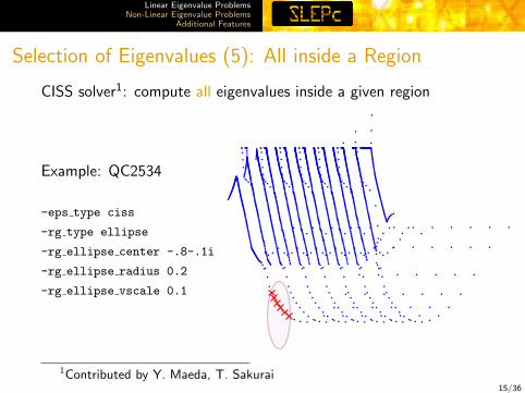
Selection of Eigenvalues (5): All inside a Region
CISS solver1: compute all eigenvalues inside a given region
Example: QC2534
-eps type ciss
-rg type ellipse
-rg ellipse center -.8-.1i
-rg ellipse radius 0.2
-rg ellipse vscale 0.1
1Contributed by Y. Maeda, T. Sakurai15/36
Linear Eigenvalue ProblemsNon-Linear Eigenvalue Problems
Additional Features
Selection of Eigenvalues (5): All inside a Region
Example: MHD1280 with CISS
I Alfven spectra: eigenvalues inintersection of the branches
Arbitrary selection: apply criterion to an arbitrary user-definedfunction φ(λ, x) instead of just λ
17/36
Linear Eigenvalue ProblemsNon-Linear Eigenvalue Problems
Additional Features
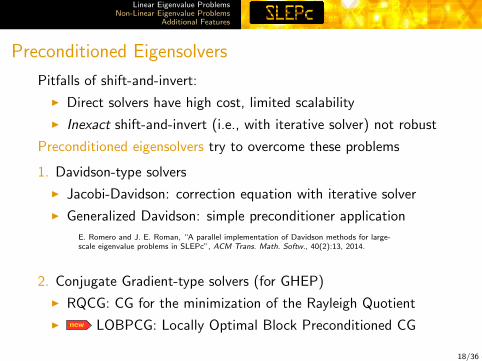
Preconditioned Eigensolvers
Pitfalls of shift-and-invert:
I Direct solvers have high cost, limited scalability
I Inexact shift-and-invert (i.e., with iterative solver) not robust
Preconditioned eigensolvers try to overcome these problems
1. Davidson-type solvers
I Jacobi-Davidson: correction equation with iterative solver
I Generalized Davidson: simple preconditioner application
E. Romero and J. E. Roman, “A parallel implementation of Davidson methods for large-scale eigenvalue problems in SLEPc”, ACM Trans. Math. Softw., 40(2):13, 2014.
2. Conjugate Gradient-type solvers (for GHEP)
I RQCG: CG for the minimization of the Rayleigh Quotient
I new LOBPCG: Locally Optimal Block Preconditioned CG
18/36
Linear Eigenvalue ProblemsNon-Linear Eigenvalue Problems
Additional Features
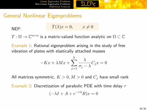
Nonlinear Eigenproblems
Increasing interest in nonlinear eigenvalue problems arising in manyapplication domains
I Structural analysis with damping effects
I Vibro-acoustics (fluid-structure interaction)
I Linear stability of fluid flows
Problem types
I QEP: quadratic eigenproblem, (λ2M + λC +K)x = 0
I PEP: polynomial eigenproblem, P (λ)x = 0
I REP: rational eigenproblem, P (λ)Q(λ)−1x = 0
I NEP: general nonlinear eigenproblem, T (λ)x = 0
Test cases available in the NLEVP collection [Betcke et al. 2013]
20/36
Linear Eigenvalue ProblemsNon-Linear Eigenvalue Problems
Additional Features
Polynomial Eigenproblems via Linearization
PEP: P (λ)x = 0
Monomial basis: P (λ) = A0 +A1λ+A2λ2 + · · ·+Adλ
d
Companion linearization: L(λ) = L0 − λL1, with L(λ)y = 0 and
L0=
I
. . .
I−A0 −A1 · · · −Ad−1
L1=
I
. . .
IAd
y=
xxλ...
xλd−1
Compute an eigenpair (y, λ) of L(λ), then extract x from y
I Pros: can leverage existing linear eigensolvers (PEPLINEAR)
I Cons: dimension of linearized problem is dn
21/36
Linear Eigenvalue ProblemsNon-Linear Eigenvalue Problems
Additional Features
PEP: Krylov Methods with Compact Representation
Arnoldi relation: SVj =[Vj v
]Hj , S := L−11 L0
Write Arnoldi vectors as v = vec[v0, . . . , vd−1
]Block structure of S allows an implicit representation of the basis
I Q-Arnoldi: V i+1j =
[V ij vi
]Hj
I TOAR:[V ij vi
]= Uj+d
[Gij gi
]Arnoldi relation in the compact representation:
S(Id ⊗ Uj+d−1)Gj = (Id ⊗ Uj+d)[Gj g
]Hj
PEPTOAR is the default solver
I Memory-efficient (also in terms of computational cost)
I Many features: restart, locking, scaling, extraction, refinement
C. Campos and J. E. Roman, “Parallel Krylov solvers for the polynomial eigenvalue problemin SLEPc”, submitted, 2015.
22/36
Linear Eigenvalue ProblemsNon-Linear Eigenvalue Problems
Additional Features
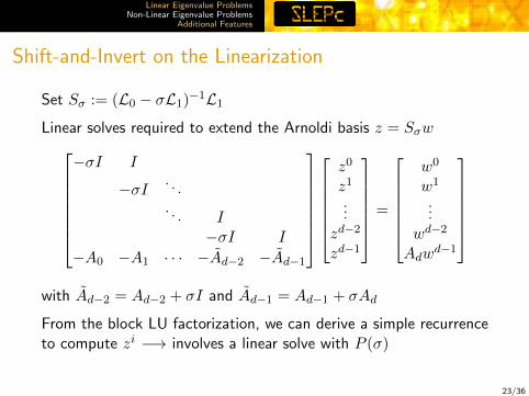
Shift-and-Invert on the Linearization
Set Sσ := (L0 − σL1)−1L1Linear solves required to extend the Arnoldi basis z = Sσw−σI I
−σI . . .. . . I
−σI I
−A0 −A1 · · · −Ad−2 −Ad−1
z0
z1
...zd−2
zd−1
=
w0
w1
...wd−2
Adwd−1
with Ad−2 = Ad−2 + σI and Ad−1 = Ad−1 + σAd
From the block LU factorization, we can derive a simple recurrenceto compute zi −→ involves a linear solve with P (σ)
23/36
Linear Eigenvalue ProblemsNon-Linear Eigenvalue Problems
Additional Features
Quantum Dot Simulation
3D pyramidal quantum dot discretized with finite volumes
Tsung-Min Hwang et al. (2004). “Numerical Simulationof Three Dimensional Pyramid Quantum Dot,” Journal ofComputational Physics, 196(1): 208-232.