82
Slide 1 Computers for the PostPC Era Dave Patterson University of California at Berkeley [email protected] http://iram.cs.berkeley.edu/ http://iram.CS.Berkeley.EDU/istore/ March 2001
| Date post: | 21-Dec-2015 |
| Category: |
Documents |
| View: | 216 times |
| Download: | 0 times |
Slide 1
Computers for the PostPC Era
Dave PattersonUniversity of California at Berkeley
http://iram.cs.berkeley.edu/http://iram.CS.Berkeley.EDU/istore/
March 2001

Slide 2
Perspective on Post-PC Era
• PostPC Era will be driven by 2 technologies:
1) Mobile Consumer Devices–e.g., successor to
cell phone, PDA, wearable computers
2) Infrastructure to Support such Devices–e.g., successor to Big Fat Web Servers,
Database Servers (Yahoo+, Amazon+, …)
Slide 3
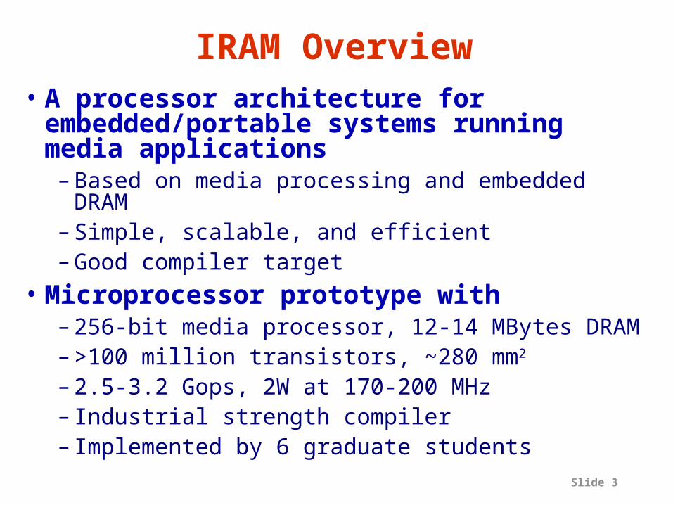
IRAM Overview• A processor architecture for
embedded/portable systems running media applications– Based on media processing and embedded DRAM– Simple, scalable, and efficient– Good compiler target
• Microprocessor prototype with– 256-bit media processor, 12-14 MBytes DRAM– >100 million transistors, ~280 mm2
– 2.5-3.2 Gops, 2W at 170-200 MHz– Industrial strength compiler– Implemented by 6 graduate students
Slide 4
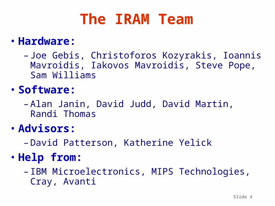
The IRAM Team• Hardware:
– Joe Gebis, Christoforos Kozyrakis, Ioannis Mavroidis, Iakovos Mavroidis, Steve Pope, Sam Williams
• Software: – Alan Janin, David Judd, David Martin, Randi
Thomas
• Advisors:– David Patterson, Katherine Yelick
• Help from:– IBM Microelectronics, MIPS Technologies, Cray,
Avanti

Slide 5
PostPC processor applications• Multimedia processing; (“90% desktop
cycles”)– image/video processing, voice/pattern recognition, 3D
graphics, animation, digital music, encryption– narrow data types, streaming data, real-time response
• Embedded and portable systems– notebooks, PDAs, digital cameras, cellular phones,
pagers, game consoles, set-top boxes– limited chip count, limited power/energy budget
• Significantly different environment from that of workstations and servers
• And larger: ‘99 32-bit microprocessor market 386 million for Embedded, 160 million for PCs;>500M cell phones in 2001

Slide 6
Motivation and Goals• Processor features for PostPC systems:
– High performance on demand for multimedia without continuous high power consumption
– Tolerance to memory latency – Scalable– Mature, HLL-based software model
• Design a prototype processor chip– Complete proof of concept– Explore detailed architecture and design issues– Motivation for software development

Slide 7
Key Technologies• Media processing
– High performance on demand for media processing
– Low power for issue and control logic– Low design complexity– Well understood compiler technology
• Embedded DRAM– High bandwidth for media processing– Low power/energy for memory accesses– “System on a chip”

Slide 8
Potential Multimedia Architecture
• “New” model: VSIW=Very Short Instruction Word!– Compact: Describe N operations with 1 short instruct.– Predictable (real-time) perf. vs. statistical perf. (cache)– Multimedia ready: choose N*64b, 2N*32b, 4N*16b– Easy to get high performance; N operations:
» are independent» use same functional unit» access disjoint registers» access registers in same order as previous instructions» access contiguous memory words or known pattern» hides memory latency (and any other latency)
– Compiler technology already developed, for sale!

Slide 9
Operation & Instruction Count: RISC v. “VSIW” Processor
(from F. Quintana, U. Barcelona.)
Spec92fp Operations (M) Instructions (M)
Program RISC VSIW R / V RISC VSIW R / Vswim256 115 95 1.1x 115 0.8 142xhydro2d 58 40 1.4x 58 0.8 71xnasa7 69 41 1.7x 69 2.2 31xsu2cor 51 35 1.4x 51 1.8 29xtomcatv 15 10 1.4x 15 1.3 11xwave5 27 25 1.1x 27 7.2 4xmdljdp2 32 52 0.6x 32 15.8 2x
VSIW reduces ops by 1.2X, instructions by 20X!
Slide 10
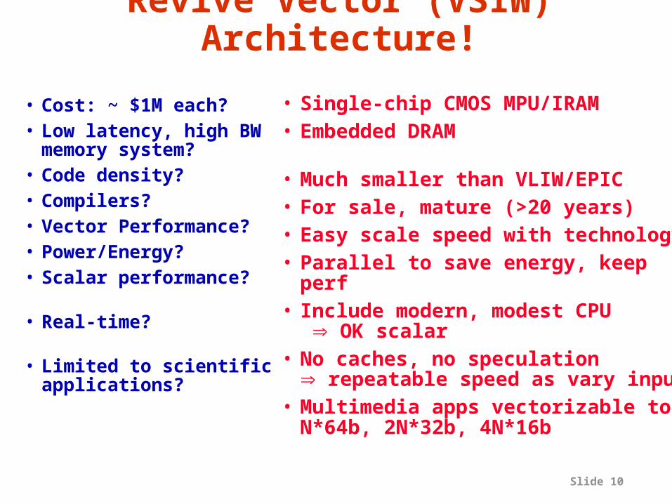
Revive Vector (VSIW) Architecture!
• Cost: ~ $1M each?• Low latency, high BW
memory system?• Code density?• Compilers?• Vector Performance?• Power/Energy?• Scalar performance?
• Real-time?
• Limited to scientific applications?
• Single-chip CMOS MPU/IRAM• Embedded DRAM
• Much smaller than VLIW/EPIC• For sale, mature (>20 years)• Easy scale speed with technology• Parallel to save energy, keep perf• Include modern, modest CPU
OK scalar• No caches, no speculation
repeatable speed as vary input • Multimedia apps vectorizable too:
N*64b, 2N*32b, 4N*16b
Slide 11
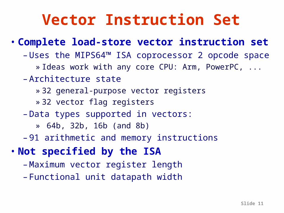
Vector Instruction Set• Complete load-store vector instruction set
– Uses the MIPS64™ ISA coprocessor 2 opcode space» Ideas work with any core CPU: Arm, PowerPC, ...
– Architecture state» 32 general-purpose vector registers» 32 vector flag registers
– Data types supported in vectors:» 64b, 32b, 16b (and 8b)
– 91 arithmetic and memory instructions
• Not specified by the ISA– Maximum vector register length– Functional unit datapath width

Slide 12
Vector IRAM ISA Summary
s.intu.ints.fpd.fp
.v.vv.vs.sv
s.intu.int
unit strideconstant stride
indexed
loadstore
VectorALU
VectorMemory
Scalar MIPS64 scalar instruction set
alu op
8163264
•91 instructions•660 opcodes
ALU operations: integer, floating-point, convert, logical, vector processing, flag processing

Slide 13
Support for DSP
• Support for fixed-point numbers, saturation, rounding modes
• Simple instructions for intra-register permutations for reductions and butterfly operations– High performance for dot-products and FFT
without the complexity of a random permutation
sat
Round
a
w
y
z
+*
x
n/2
n/2
n
n
n
n
Slide 14
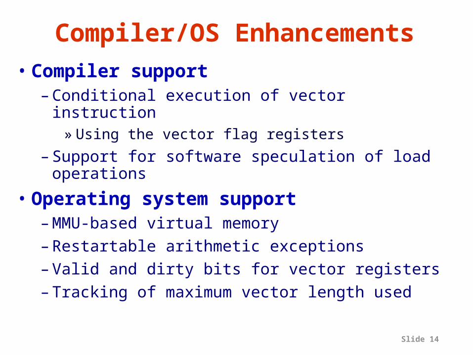
Compiler/OS Enhancements• Compiler support
– Conditional execution of vector instruction» Using the vector flag registers
– Support for software speculation of load operations
• Operating system support– MMU-based virtual memory– Restartable arithmetic exceptions– Valid and dirty bits for vector registers– Tracking of maximum vector length used

Slide 15
VIRAM Prototype Architecture
MIPS64™
5Kc Core
Instr. Cache (8KB)
Data Cache (8KB)
CP
IF
FPU
Vector Register File (8KB)
Flag Register File (512B)
Flag Unit 0
Memory Unit
DMA256b
Memory Crossbar
256b 256b
64b
DRAM0
(2MB)
DRAM1
(2MB)
DRAM7
(2MB)…
SysAD IF
64b
ArithmeticUnit 0
ArithmeticUnit 1
Flag Unit 1
JTAG
JTAG IF
TLB

Slide 16
Architecture Details (1)• MIPS64™ 5Kc core (200 MHz)
– Single-issue core with 6 stage pipeline– 8 KByte, direct-map instruction and data caches– Single-precision scalar FPU
• Vector unit (200 MHz)– 8 KByte register file (32 64b elements per register)– 4 functional units:
» 2 arithmetic (1 FP), 2 flag processing» 256b datapaths per functional unit
– Memory unit» 4 address generators for strided/indexed accesses» 2-level TLB structure: 4-ported, 4-entry microTLB and
single-ported, 32-entry main TLB» Pipelined to sustain up to 64 pending memory accesses

Slide 17
Architecture Details (2)• Main memory system
– No SRAM cache for the vector unit– 8 2-MByte DRAM macros
» Single bank per macro, 2Kb page size» 256b synchronous, non-multiplexed I/O interface» 25ns random access time, 7.5ns page access
time
– Crossbar interconnect» 12.8 GBytes/s peak bandwidth per direction
(load/store)» Up to 5 independent addresses transmitted per
cycle
• Off-chip interface– 64b SysAD bus to external chip-set (100 MHz)– 2 channel DMA engine
Slide 18
Vector Unit Pipeline• Single-issue, in-order pipeline• Efficient for short vectors
– Pipelined instruction start-up– Full support for instruction chaining, the vector
equivalent of result forwarding
• Hides long DRAM access latency

Slide 19
Modular Vector Unit Design
• Single 64b “lane” design replicated 4 times– Reduces design and testing time– Provides a simple scaling model (up or down) without major control
or datapath redesign
• Most instructions require only intra-lane interconnect– Tolerance to interconnect delay scaling
256b
Control
64b
Xbar IF
Integer Datapath 0
Flag Reg. Elements& Datapaths
Vector Reg.Elements
FP Datapath
Integer Datapath 1
64b
Xbar IF
Integer Datapath 0
Flag Reg. Elements& Datapaths
Vector Reg.Elements
FP Datapath
Integer Datapath 1
64b
Xbar IF
Integer Datapath 0
Flag Reg. Elements& Datapaths
Vector Reg.Elements
FP Datapath
Integer Datapath 1
64b
Xbar IF
Integer Datapath 0
Flag Reg. Elements& Datapaths
Vector Reg.Elements
FP Datapath
Integer Datapath 1
Slide 20
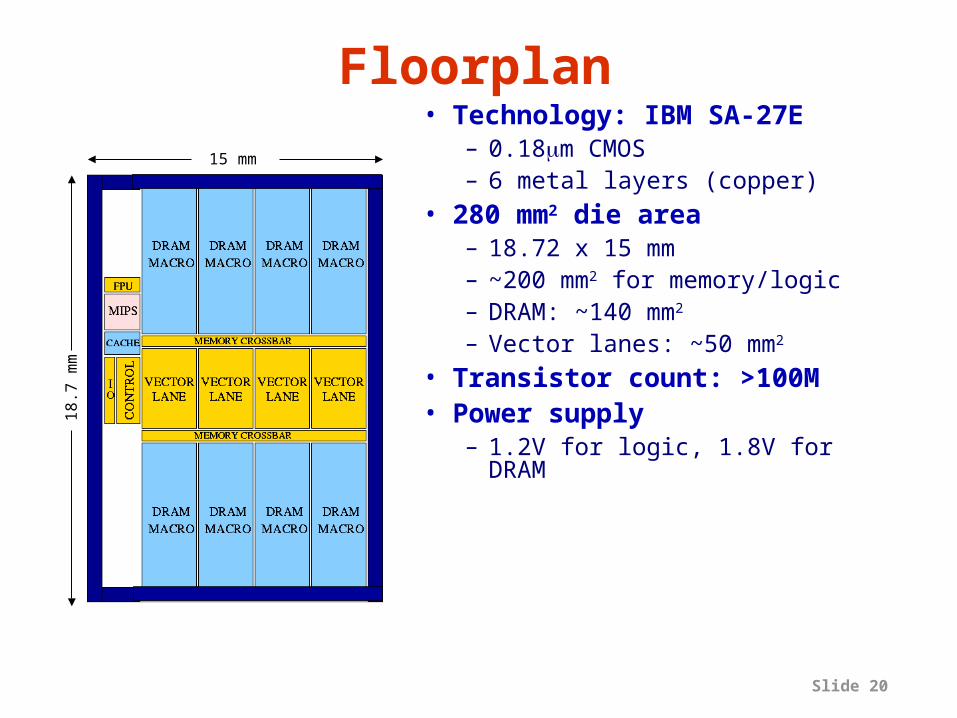
Floorplan• Technology: IBM SA-27E
– 0.18m CMOS– 6 metal layers (copper)
• 280 mm2 die area– 18.72 x 15 mm– ~200 mm2 for memory/logic– DRAM: ~140 mm2 – Vector lanes: ~50 mm2
• Transistor count: >100M• Power supply
– 1.2V for logic, 1.8V for DRAM
15 mm
18
.7 m
m

Slide 21
Alternative Floorplans (1)
“VIRAM-7MB”
4 lanes, 8 Mbytes
190 mm2
3.2 Gops at 200 MHz(32-bit ops)
“VIRAM-2Lanes”
2 lanes, 4 Mbytes
120 mm2
1.6 Gops at 200 MHz
“VIRAM-Lite”
1 lane, 2 Mbytes
60 mm2
0.8 Gops at 200 MHz

Slide 22
Power Consumption• Power saving techniques
– Low power supply for logic (1.2 V)» Possible because of the low clock rate (200 MHz)» Wide vector datapaths provide high performance
– Extensive clock gating and datapath disabling» Utilizing the explicit parallelism information of vector
instructions and conditional execution
– Simple, single-issue, in-order pipeline
• Typical power consumption: 2.0 W– MIPS core: 0.5 W – Vector unit:1.0 W (min ~0 W)– DRAM: 0.2 W (min ~0 W)– Misc.: 0.3 W (min ~0 W)

Slide 23
VIRAM Compiler
• Based on the Cray’s PDGCS production environment for vector supercomputers
• Extensive vectorization and optimization capabilities including outer loop vectorization
• No need to use special libraries or variable types for vectorization
Optimizer
C
Fortran95
C++
Frontends Code Generators
Cray’s
PDGCS
T3D/T3E
SV2/VIRAM
C90/T90/SV1

Slide 24
Compiling Media Kernels on IRAM
• The compiler generates code for narrow data widths, e.g., 16-bit integer
• Compilation model is simple, more scalable (across generations) than MMX, VIS, etc.
0
500
1000
1500
2000
2500
3000
3500
MFLO
PS
colorspace composite FIR filter
1 lane
2 lane
4 lane
8 lane
– Strided and indexed loads/stores simpler than pack/unpack
– Maximum vector length is longer than datapath width (256 bits); all lane scalings done with single executable

Slide 25
Performance: Efficiency
89.4%Average
99.6%1.59 GFLOPS1.6 GFLOPSFP VM Multiply
93.7%3.00 GOPS3.2 GOPSInteger VM Multiply
98.7%3.16 GOPS3.2 GOPSImage Convolution
96.0%3.07 GOPS3.2 GOPSColor Conversion
48.4%3.10 GOPS6.4 GOPSiDCT
100%6.40 GOPS6.4 GOPSImage Composition
% of PeakSustainedPeak
What % of peak delivered by superscalar or VLIW designs?
50%? 25%?
Slide 26
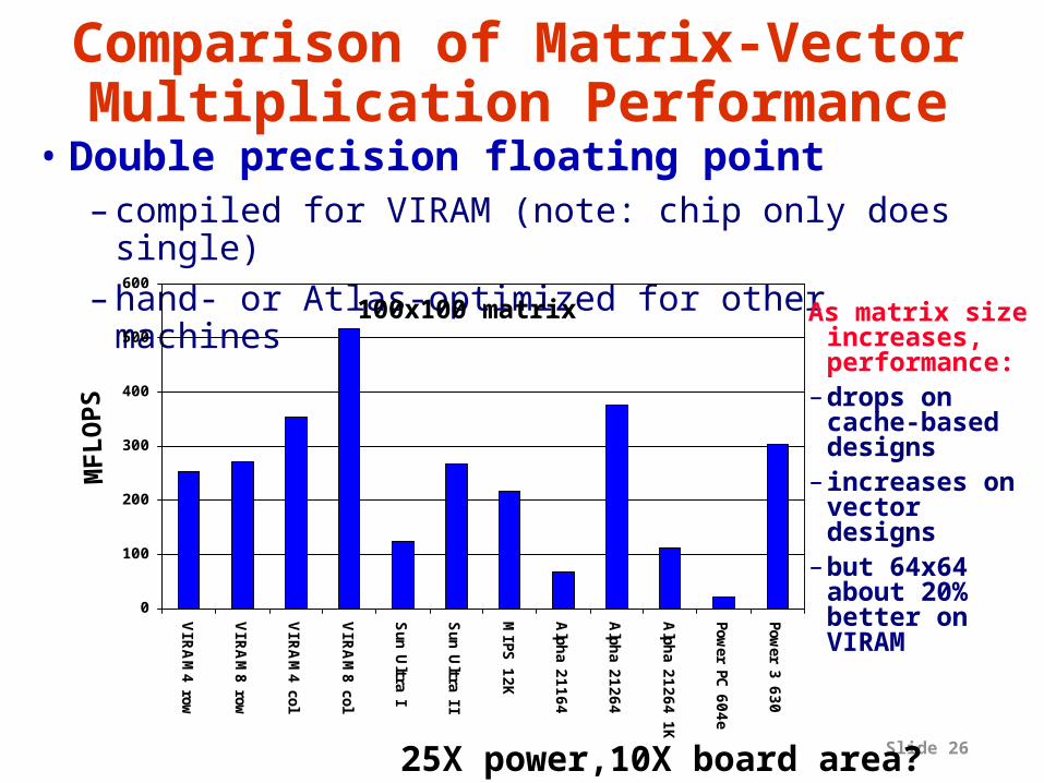
Comparison of Matrix-Vector Multiplication Performance
• Double precision floating point– compiled for VIRAM (note: chip only does single)– hand- or Atlas-optimized for other machines
0
100
200
300
400
500
600
VIR
AM
4 row
VIR
AM
8 row
VIR
AM
4 col
VIR
AM
8 col
Sun U
ltra I
Sun U
ltra II
MIPS
12K
Alph
a 21164
Alph
a 21264
Alph
a 21264 1
K
Power PC
604e
Power 3
630
As matrix size increases, performance:
– drops on cache-based designs
– increases on vector designs
– but 64x64 about 20% better on VIRAM
MFLO
PS
100x100 matrix
25X power,10X board area?
Slide 27
IRAM Statistics• 2 Watts, 3 GOPS, Multimedia ready
(including memory) AND can compile for it
• >100 Million transistors– Intel @ 50M?
• Industrial strength compilers• Tape out June 2001?• 6 grad students• Thanks to
– DARPA: fund effort– IBM: donate masks, fab– Avanti: donate CAD tools– MIPS: donate MIPS core– Cray: Compilers
Slide 28
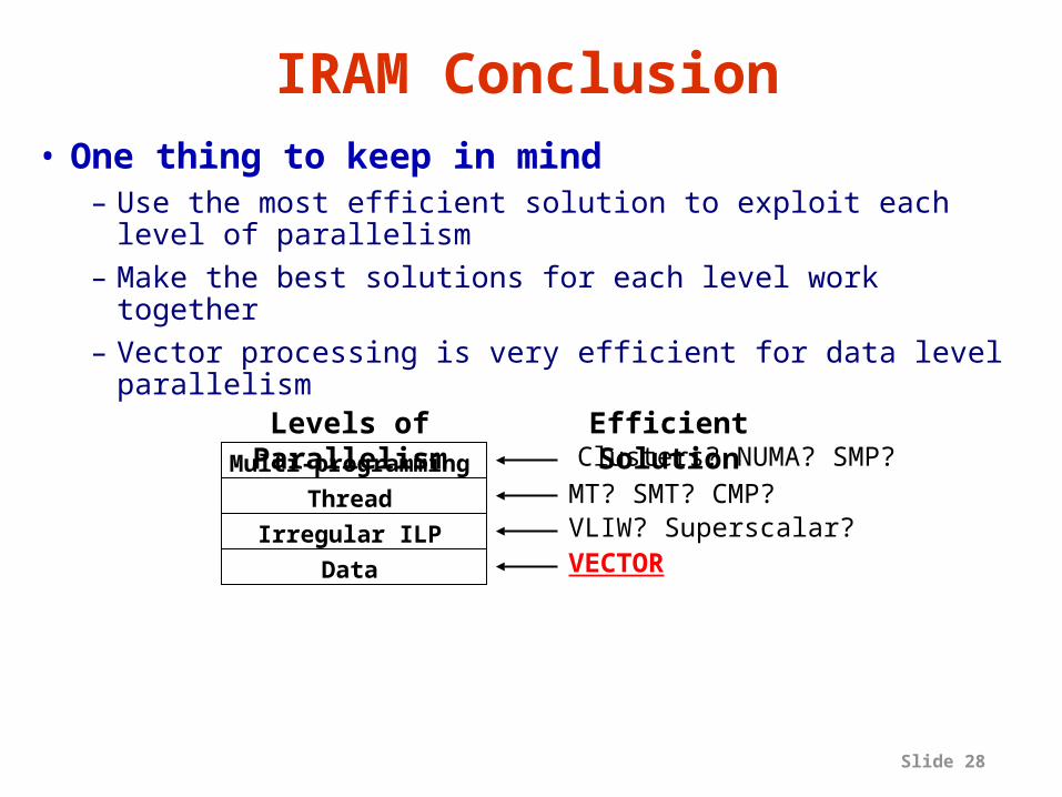
IRAM Conclusion• One thing to keep in mind
– Use the most efficient solution to exploit each level of parallelism
– Make the best solutions for each level work together– Vector processing is very efficient for data level parallelism
MT? SMT? CMP?VLIW? Superscalar?VECTOR
Clusters? NUMA? SMP?
Data
Irregular ILP
Thread
Multi-programming
Levels of Parallelism Efficient Solution
Slide 29
Goals,Assumptions of last 15 years
• Goal #1: Improve performance• Goal #2: Improve performance• Goal #3: Improve cost-performance• Assumptions
– Humans are perfect (they don’t make mistakes during installation, wiring, upgrade, maintenance or repair)
– Software will eventually be bug free (good programmers write bug-free code)
– Hardware MTBF is already very large (~100 years between failures), and will continue to increase

Slide 30
After 15 year improving Perfmance
• Availability is now a vital metric for servers!– near-100% availability is becoming mandatory
» for e-commerce, enterprise apps, online services, ISPs
– but, service outages are frequent» 65% of IT managers report that their websites were
unavailable to customers over a 6-month period•25%: 3 or more outages
– outage costs are high» NYC stockbroker: $6,500,000/hr» EBay: $225,000/hr» Amazon.com: $180,000/hr» social effects: negative press, loss of customers who
“click over” to competitorSource: InternetWeek 4/3/2000

Slide 31
ISTORE as an Example of Storage System of the Future
• Availability, Maintainability, and Evolutionary growth key challenges for storage systems
– Maintenance Cost ~ >10X Purchase Cost per year, – Even 2X purchase cost for 1/2 maintenance cost wins– AME improvement enables even larger systems
• ISTORE also cost-performance advantages– Better space, power/cooling costs
($ @ collocation site)– More MIPS, cheaper MIPS, no bus bottlenecks– Single interconnect, supports evolution of technology,
single network technology to maintain/understand• Match to future software storage services
– Future storage service software target clusters

Slide 32
Jim Gray: Trouble-Free Systems
• Manager – Sets goals– Sets policy– Sets budget– System does the rest.
• Everyone is a CIO (Chief Information Officer)
• Build a system – used by millions of people each day– Administered and managed by a ½ time person.
» On hardware fault, order replacement part» On overload, order additional equipment» Upgrade hardware and software automatically.
“What Next? A dozen remaining IT problems”
Turing Award Lecture, FCRC,
May 1999Jim GrayMicrosoft

Slide 33
Hennessy: What Should the “New World” Focus Be?• Availability
– Both appliance & service• Maintainability
– Two functions:» Enhancing availability by preventing failure» Ease of SW and HW upgrades
• Scalability– Especially of service
• Cost– per device and per service transaction
• Performance– Remains important, but its not SPECint
“Back to the Future: Time to Return to Longstanding
Problems in Computer Systems?” Keynote address,
FCRC, May 1999
John HennessyStanford

Slide 34
The real scalability problems: AME
• Availability– systems should continue to meet quality of service
goals despite hardware and software failures
• Maintainability– systems should require only minimal ongoing human
administration, regardless of scale or complexity: Today, cost of maintenance = 10-100 cost of purchase
• Evolutionary Growth– systems should evolve gracefully in terms of
performance, maintainability, and availability as they are grown/upgraded/expanded
• These are problems at today’s scales, and will only get worse as systems grow

Slide 35
Lessons learned from Past Projects for which might help
AME• Know how to improve performance (and cost)
– Run system against workload, measure, innovate, repeat– Benchmarks standardize workloads, lead to competition,
evaluate alternatives; turns debates into numbers• Major improvements in Hardware Reliability
– 1990 Disks 50,000 hour MTBF to 1,200,000 in 2000– PC motherboards from 100,000 to 1,000,000 hours
• Yet Everything has an error rate– Well designed and manufactured HW: >1% fail/year– Well designed and tested SW: > 1 bug / 1000 lines– Well trained, rested people doing routine tasks: >1%??– Well run collocation site (e.g., Exodus):
1 power failure per year, 1 network outage per year

Slide 36
Lessons learned from Past Projects for AME
• Maintenance of machines (with state) expensive– ~10X cost of HW per year– Stateless machines can be trivial to maintain
(Hotmail)
• System administration primarily keeps system available– System + clever human = uptime– Also plan for growth, fix performance bugs, do
backup
• Software upgrades necessary, dangerous– SW bugs fixed, new features added, but stability?– Admins try to skip upgrades, be the last to use one
Slide 37
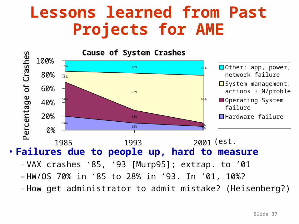
Cause of System Crashes
20%10%
5%
50%
18%
5%
15%
53%
69%
15% 18% 21%
0%
20%
40%
60%
80%
100%
1985 1993 2001
Other: app, power, network failure
System management: actions + N/problem
Operating Systemfailure
Hardware failure
(est.)
Lessons learned from Past Projects for AME
• Failures due to people up, hard to measure– VAX crashes ‘85, ‘93 [Murp95]; extrap. to ‘01– HW/OS 70% in ‘85 to 28% in ‘93. In ‘01, 10%?– How get administrator to admit mistake? (Heisenberg?)
Slide 38
Lessons learned from Past Projects for AME
• Components fail slowly– Disks, Memory, Software give indications before fail
(Interfaces don’t pass along this information)
• Component performance varies– Disk inner track vs. outer track: 1.8X Bandwidth– Refresh of DRAM– Daemon processes in nodes of cluster– Error correction, retry on some storage accesses– Maintenance events in switches
(Interfaces don’t pass along this information)

Slide 39
Lessons Learned from Other Fields
Common threads in accidents ~3 Mile Island1.More multiple failures than you believe
possible (like the birthday paradox?)2. Operators cannot fully understand system
because errors in implementation, and errors in measurement system. Also complex interactions that are hard to predict
3.Tendency to blame operators afterwards (60-80%), but they must operate with missing, wrong information
4.The systems are never all working fully properly: bad indicator lights, sensors out, things in repair
5.Systems that kick in when trouble often flawed. A 3 Mile Island problem 2 valves left in the wrong position-they were symmetric parts of a redundant system used only in an emergency. The fact that the facility runs under normal operation masks these errors
Charles Perrow, Normal Accidents: Living with High Risk Technologies, Perseus Books, 1990

Slide 40
An Approach to AME "If a problem has no solution, it may not be a problem, but a fact, not be solved, but to be coped with over time."
Shimon Peres, quoted in Rumsfeld's Rules
• Rather than aim towards (or expect) perfect hardware, software, & people, assume flaws
• Focus on Mean Time To Repair (MTTR), for whole system including people who maintain it– Availability = MTTR / MTBF, so
1/10th MTTR just as valuable as 10X MTBF– Improving MTTR and hence availability should improve
cost of administration/maintenance as well

Slide 41
An Approach to AME
• 4 Parts to Time to Repair: 1) Time to detect error, 2) Time to pinpoint error
(“root cause analysis”), 3) Time to chose try several possible solutions fixes error, and 4) Time to fix error

Slide 42
An Approach to AME
1) Time to Detect errors• Include interfaces that report
faults/errors from components– May allow application/system to
predict/identify failures
• Periodic insertion of test inputs into system with known results vs. wait for failure reports

Slide 43
An Approach to AME
2) Time to Pinpoint error • Error checking at edges of each
component• Design each component so it can be
isolated and given test inputs to see if performs
• Keep history of failure symptoms/reasons and recent behavior (“root cause analysis”)

Slide 44
An Approach to AME
• 3) Time to try possible solutions: • History of errors/solutions• Undo of any repair to allow trial of
possible solutions– Support of snapshots, transactions/logging
fundamental in system– Since disk capacity, bandwidth is fastest
growing technology, use it to improve repair?– Caching at many levels of systems provides
redundancy that may be used for transactions?

Slide 45
An Approach to AME 4) Time to fix error: • Create Repair benchmarks
– Competition leads to improved MTTR• Include interfaces that allow Repair
events to be systematically tested– Predictable fault insertion allows debugging of
repair as well as benchmarking MTTR• Since people make mistakes during
repair, “undo” for any maintenance event– Replace wrong disk in RAID system on a failure;
undo and replace bad disk without losing info– Undo a software upgrade

Slide 46
Other Ideas for AME• Use interfaces that report, expect
performance variability vs. expect consistency?– Especially when trying to repair– Example: work allocated per server based on recent
performance vs. based on expected performance
• Queued interfaces, flow control accommodate performance variability, failures?– Example: queued communication vs. Barrier/Bulk
Synchronous communication for distributed program

Slide 47
Overview towards AME• New foundation to reduce MTTR
– Cope with fact that people, SW, HW fail (Peres)– Transactions/snapshots to undo failures, bad repairs– Repair benchmarks to evaluate MTTR innovations– Interfaces to allow error insertion, input insertion,
report module errors, report module performance– Module I/O error checking and module isolation– Log errors and solutions for root cause analysis, give
ranking to potential solutions to problem problem
• Significantly reducing MTTR (HW/SW/LW) => Significantly increased availability

Slide 48
Benchmarking availability• Results
– graphical depiction of quality of service behavior
– graph visually describes availability behavior– can extract quantitative results for:
» degree of quality of service degradation» repair time (measures maintainability)» etc.
Repair Time
QoS degradationinjected
fault
normal behavior(99% conf.)

Slide 49
Time (minutes)0 10 20 30 40 50 60 70 80 90 100 110
80
100
120
140
160
0
1
2
Hits/sec# failures tolerated
0 10 20 30 40 50 60 70 80 90 100 110
Hit
s p
er s
eco
nd
190
195
200
205
210
215
220
#fai
lure
s t
ole
rate
d
0
1
2
Reconstruction
Reconstruction
Example: single-fault in SW RAID
• Compares Linux and Solaris reconstruction– Linux: minimal performance impact but longer window
of vulnerability to second fault– Solaris: large perf. impact but restores redundancy fast– Windows: does not auto-reconstruct!
Linux
Solaris

Slide 50
Software RAID: QoS behavior• Response to transient errors
– Linux is paranoid with respect to transients» stops using affected disk (and reconstructs) on any
error, transient or not– Solaris and Windows are more forgiving
» both ignore most benign/transient faults– neither policy is ideal!
» need a hybrid that detects streams of transients
SolarisLinux

Slide 51
Software RAID: QoS behavior• Response to double-fault scenario
– a double fault results in unrecoverable loss of data on the RAID volume
– Linux: blocked access to volume– Windows: blocked access to volume– Solaris: silently continued using volume,
delivering fabricated data to application!» clear violation of RAID availability semantics» resulted in corrupted file system and garbage data
at the application level» this undocumented policy has serious availability
implications for applications

Slide 52
Software RAID: maintainability
• Human error rates– subjects attempt to repair RAID disk failures
» by replacing broken disk and reconstructing data
– each subject repeated task several times– data aggregated across 5 subjects
Error type Windows
Solaris Linux
Fatal Data Loss
Unsuccessful Repair
System ignored fatal input
User Error – Intervention Required
User Error – User Recovered Total number of trials 35 33 31

Slide 53
Example Server:ISTORE-1 hardware platform
• 64-node x86-based cluster, 1.1TB storage– cluster nodes are plug-and-play, intelligent, network-
attached storage “bricks”»a single field-replaceable unit to simplify
maintenance– each node is a full x86 PC w/256MB DRAM, 18GB disk– more CPU than NAS; fewer disks/node than cluster
Intelligent Disk “Brick”Portable PC CPU: Pentium II/266 + DRAM
Redundant NICs (4 100 Mb/s links)Diagnostic Processor
Disk
Half-height canister
ISTORE Chassis64 nodes, 8 per tray2 levels of switches•20 100 Mbit/s•2 1 Gbit/sEnvironment Monitoring:UPS, redundant PS,fans, heat and vibration sensors...

Slide 54
ISTORE Brick Node• Pentium-II/266MHz• 18 GB SCSI (or IDE) disk• 4x100Mb Ethernet,256 MB DRAM• m68k diagnostic processor & CAN diagnostic network• Includes Temperature, Motion Sensors, Fault
injection, network isolation• Packaged in standard half-height RAID array canister

Slide 55
ISTORE Cost Performance• MIPS: Abundant Cheap, Low Power
– 1 Processor per disk, amortizing disk enclosure, power supply, cabling, cooling vs. 1 CPU per 8 disks
– Embedded processors 2/3 perf, 1/5 cost, power?• No Bus Bottleneck
– 1 CPU, 1 memory bus, 1 I/O bus, 1 controller, 1 disk
vs. 1-2 CPUs, 1 memory bus, 1-2 I/O buses, 2-4 controllers, 4-16 disks
• Co-location sites (e.g., Exodus) offer space, expandable bandwidth, stable power– Charge ~$1000/month per rack ( ~ 10 sq. ft.).
+ $200 per extra 20 amp circuit
Density-optimized systems (size, cooling) vs. SPEC optimized systems @ 100s watts
Slide 56
Common Question: RAID?• Switched Network sufficient for all
types of communication, including redundancy– Hierarchy of buses is generally not superior to
switched network
• Veritas, others offer software RAID 5 and software Mirroring (RAID 1)
• Another use of processor per disk
Slide 57
Initial Applications• Future: services over WWW• Initial ISTORE apps targets are services
– information retrieval for multimedia data (XML storage?)
» self-scrubbing data structures, structuring performance-robust distributed computation
» Example: home video server using XML interfaces– email service?
» statistical identification of normal behavior» Undo of upgrade
• ISTORE-1 is not one super-system that demonstrates all techniques, but an example– Initially provide middleware, library to support AME

Slide 58
A glimpse into the future?• System-on-a-chip enables computer,
memory, redundant network interfaces without significantly increasing size of disk
• ISTORE HW in 5 years:– 2006 brick: System On a Chip
integrated with MicroDrive » 9GB disk, 50 MB/sec from disk» connected via crossbar switch» From brick to “domino”
– If low power, 10,000 nodes fit into one rack!
• O(10,000) scale is our ultimate design point

Slide 59
Conclusion #1: ISTORE as Storage System of the Future
• Availability, Maintainability, and Evolutionary growth key challenges for
storage systems– Maintenance Cost ~ 10X Purchase Cost per year, so
over 5 year product life, ~ 95% of cost of ownership– Even 2X purchase cost for 1/2 maintenance cost wins– AME improvement enables even larger systems
• ISTORE has cost-performance advantages– Better space, power/cooling costs ($@colocation site)– More MIPS, cheaper MIPS, no bus bottlenecks– Single interconnect, supports evolution of technology,
single network technology to maintain/understand• Match to future software storage services
– Future storage service software target clusters

Slide 60
Conclusion #2: IRAM and ISTORE Vision
• Integrated processor in memory provides efficient access to high memory bandwidth
• Two “Post-PC” applications:– IRAM: Single chip system
for embedded and portable applications
» Target media processing (speech, images, video, audio)
– ISTORE: Building block when combined with disk for storage and retrieval servers
» Up to 10K nodes in one rack
» Non-IRAM prototype addresses key scaling issues: availability, manageability, evolution
Photo from Itsy, Inc.

Slide 61
Questions?
Contact us if you’re interested:email: [email protected]
http://iram.cs.berkeley.edu/ http://iram.cs.berkeley.edu/istore
“If it’s important, how can you say if it’s impossible if you don’t try?”
Jean Morreau, a founder of European Union

Slide 62
ISTORE-1 Brick• Webster’s Dictionary:
“brick: a handy-sized unit of building or paving material typically being rectangular and about 2 1/4 x 3 3/4 x 8 inches”
• ISTORE-1 Brick: 2 x 4 x 11 inches (1.3x)– Single physical form factor, fixed cooling required,
compatible network interface to simplify physical maintenance, scaling over time
– Contents should evolve over time: contains most cost effective MPU, DRAM, disk, compatible NI
– If useful, could have special bricks (e.g., DRAM rich, disk poor)
– Suggests network that will last, evolve: Ethernet

Slide 63
Embedded DRAM in the News• Sony ISSCC 2001• 462-mm2 chip with 256-Mbit of on-chip
embedded DRAM (8X Emotion engine in PS/2)– 0.18-micron design rules – 21.7 x 21.3-mm and contains 287.5 million
transistors
• 2,000-bit internal buses can deliver 48 gigabytes per second of bandwidth
• Demonstrated at Siggraph 2000• Used in multiprocessor graphics
system?

Slide 64
Cost of Bandwidth, Safety• Network bandwidth cost is significant
– 1000 Mbit/sec/month => $6,000,000/year
• Security will increase in importance for storage service providers
• XML => server format conversion for gadgets
=> Storage systems of future need greater computing ability– Compress to reduce cost of network bandwidth 3X;
save $4M/year?– Encrypt to protect information in transit for B2B
=> Increasing processing/disk for future storage apps

Slide 65
Disk Limit: Bus HierarchyCPU Memory
bus
Memory
External I/O bus
(SCSI)
(PCI)
Internal I/O bus
• Data rate vs. Disk rate– SCSI: Ultra3 (80 MHz),
Wide (16 bit): 160 MByte/s– FC-AL: 1 Gbit/s = 125 MByte/s
Use only 50% of a busCommand overhead (~ 20%)Queuing Theory (< 70%)
(15 disks/bus)
Storage Area Network
(FC-AL)
Server
DiskArray
Mem
RAID bus

Slide 66
Vector Vs. SIMD
Simple scalar loads; multiple instructions needed to load a vector
Strided and indexed vector load and store instructions
Short vectors must be aligned in memory; otherwise multiple instructions needed to load them
No alignment restriction for vectors; only individual elements must be aligned to their width
Wide datapaths can be used either after changing the ISA or after changing the issue width
Wide datapaths can be used without changes in ISA or issue logic redesign
One instruction keeps one datapath busy for one cycle
One instruction keeps multiple datapaths busy for many cycles
SIMDVector

Slide 67
Performance: FFT (1)
FFT (Floating-point, 1024 points)
36
16.825
69
92
124.3
0
40
80
120
160
Ex
ec
uti
on
Tim
e (
us
ec
)
VIRAM
Pathfinder-2
Wildstar
TigerSHARC
ADSP-21160
TMS320C6701

Slide 68
Performance: FFT (2)
FFT (Fixed-point, 256 points)
7.2 8.1 9 7.3
87
151
0
40
80
120
160
Ex
ec
uti
on
Tim
e (
us
ec
)
VIRAM
Pathfinder-1
Carmel
TigerSHARC
PPC 604E
Pentium

Slide 69
Vector Vs. SIMD: Example• Simple example: conversion from RGB
to YUV
Y = [( 9798*R + 19235*G + 3736*B) / 32768]
U = [(-4784*R - 9437*G + 4221*B) / 32768] + 128
V = [(20218*R – 16941*G – 3277*B) / 32768] + 128

Slide 70
VIRAM Code (22 instrs, 16 arith)
RGBtoYUV:
vlds.u.b r_v, r_addr, stride3, addr_inc # load R
vlds.u.b g_v, g_addr, stride3, addr_inc # load G
vlds.u.b b_v, b_addr, stride3, addr_inc # load B
xlmul.u.sv o1_v, t0_s, r_v # calculate Y
xlmadd.u.sv o1_v, t1_s, g_v
xlmadd.u.sv o1_v, t2_s, b_v
vsra.vs o1_v, o1_v, s_s
xlmul.u.sv o2_v, t3_s, r_v # calculate U
xlmadd.u.sv o2_v, t4_s, g_v
xlmadd.u.sv o2_v, t5_s, b_v
vsra.vs o2_v, o2_v, s_s
vadd.sv o2_v, a_s, o2_v
xlmul.u.sv o3_v, t6_s, r_v # calculate V
xlmadd.u.sv o3_v, t7_s, g_v
xlmadd.u.sv o3_v, t8_s, b_v
vsra.vs o3_v, o3_v, s_s
vadd.sv o3_v, a_s, o3_v
vsts.b o1_v, y_addr, stride3, addr_inc # store Y
vsts.b o2_v, u_addr, stride3, addr_inc # store U
vsts.b o3_v, v_addr, stride3, addr_inc # store V
subu pix_s,pix_s, len_s
bnez pix_s, RGBtoYUV

Slide 71
MMX Code (part 1)RGBtoYUV:
movq mm1, [eax]
pxor mm6, mm6
movq mm0, mm1
psrlq mm1, 16
punpcklbw mm0, ZEROS
movq mm7, mm1
punpcklbw mm1, ZEROS
movq mm2, mm0
pmaddwd mm0, YR0GR
movq mm3, mm1
pmaddwd mm1, YBG0B
movq mm4, mm2
pmaddwd mm2, UR0GR
movq mm5, mm3
pmaddwd mm3, UBG0B
punpckhbw mm7, mm6;
pmaddwd mm4, VR0GR
paddd mm0, mm1
pmaddwd mm5, VBG0B
movq mm1, 8[eax]
paddd mm2, mm3
movq mm6, mm1
paddd mm4, mm5
movq mm5, mm1
psllq mm1, 32
paddd mm1, mm7
punpckhbw mm6, ZEROS
movq mm3, mm1
pmaddwd mm1, YR0GR
movq mm7, mm5
pmaddwd mm5, YBG0B
psrad mm0, 15
movq TEMP0, mm6
movq mm6, mm3
pmaddwd mm6, UR0GR
psrad mm2, 15
paddd mm1, mm5
movq mm5, mm7
pmaddwd mm7, UBG0B
psrad mm1, 15
pmaddwd mm3, VR0GR
packssdw mm0, mm1
pmaddwd mm5, VBG0B
psrad mm4, 15
movq mm1, 16[eax]

Slide 72
MMX Code (part 2) paddd mm6, mm7
movq mm7, mm1
psrad mm6, 15
paddd mm3, mm5
psllq mm7, 16
movq mm5, mm7
psrad mm3, 15
movq TEMPY, mm0
packssdw mm2, mm6
movq mm0, TEMP0
punpcklbw mm7, ZEROS
movq mm6, mm0
movq TEMPU, mm2
psrlq mm0, 32
paddw mm7, mm0
movq mm2, mm6
pmaddwd mm2, YR0GR
movq mm0, mm7
pmaddwd mm7, YBG0B
packssdw mm4, mm3
add eax, 24
add edx, 8
movq TEMPV, mm4
movq mm4, mm6
pmaddwd mm6, UR0GR
movq mm3, mm0
pmaddwd mm0, UBG0B
paddd mm2, mm7
pmaddwd mm4,
pxor mm7, mm7
pmaddwd mm3, VBG0B
punpckhbw mm1,
paddd mm0, mm6
movq mm6, mm1
pmaddwd mm6, YBG0B
punpckhbw mm5,
movq mm7, mm5
paddd mm3, mm4
pmaddwd mm5, YR0GR
movq mm4, mm1
pmaddwd mm4, UBG0B
psrad mm0, 15
paddd mm0, OFFSETW
psrad mm2, 15
paddd mm6, mm5
movq mm5, mm7

Slide 73
MMX Code (pt. 3: 121 instrs, 40 arith)
pmaddwd mm7, UR0GR
psrad mm3, 15
pmaddwd mm1, VBG0B
psrad mm6, 15
paddd mm4, OFFSETD
packssdw mm2, mm6
pmaddwd mm5, VR0GR
paddd mm7, mm4
psrad mm7, 15
movq mm6, TEMPY
packssdw mm0, mm7
movq mm4, TEMPU
packuswb mm6, mm2
movq mm7, OFFSETB
paddd mm1, mm5
paddw mm4, mm7
psrad mm1, 15
movq [ebx], mm6
packuswb mm4,
movq mm5, TEMPV
packssdw mm3, mm4
paddw mm5, mm7
paddw mm3, mm7
movq [ecx], mm4
packuswb mm5, mm3
add ebx, 8
add ecx, 8
movq [edx], mm5
dec edi
jnz RGBtoYUV

Slide 74
Clusters and TPC Software 8/’00
• TPC-C: 6 of Top 10 performance are clusters, including all of Top 5; 4 SMPs
• TPC-H: SMPs and NUMAs– 100 GB All SMPs (4-8 CPUs)– 300 GB All NUMAs (IBM/Compaq/HP 32-64 CPUs)
• TPC-R: All are clusters – 1000 GB :NCR World Mark 5200
• TPC-W: All web servers are clusters (IBM)

Slide 75
Clusters and TPC-C BenchmarkTop 10 TPC-C Performance (Aug. 2000) Ktpm1. Netfinity 8500R c/s Cluster4412. ProLiant X700-96P Cluster2623. ProLiant X550-96P Cluster2304. ProLiant X700-64P Cluster1805. ProLiant X550-64P Cluster1626. AS/400e 840-2420 SMP 1527. Fujitsu GP7000F Model 2000SMP 1398. RISC S/6000 Ent. S80 SMP 1399. Bull Escala EPC 2400 c/s SMP 13610. Enterprise 6500 Cluster Cluster
135

Slide 76
Cost of Storage System v. Disks
• Examples show cost of way we build current systems (2 networks, many buses, CPU, …)
Disks DisksDate Cost Main. Disks /CPU /IObus
– NCR WM: 10/97 $8.3M -- 1312 10.2 5.0– Sun 10k: 3/98 $5.2M -- 668 10.4 7.0– Sun 10k: 9/99 $6.2M$2.1M 1732 27.0 12.0– IBM Netinf: 7/00 $7.8M$1.8M 7040 55.0 9.0=>Too complicated, too heterogenous
• And Data Bases are often CPU or bus bound! – ISTORE disks per CPU: 1.0– ISTORE disks per I/O bus: 1.0

Slide 77
Common Question: Why Not Vary Number of Processors
and Disks?• Argument: if can vary numbers of each to match application, more cost-effective solution?
• Alternative Model 1: Dual Nodes + E-switches– P-node: Processor, Memory, 2 Ethernet NICs– D-node: Disk, 2 Ethernet NICs
• Response– As D-nodes running network protocol, still need processor
and memory, just smaller; how much save?– Saves processors/disks, costs more NICs/switches:
N ISTORE nodes vs. N/2 P-nodes + N D-nodes– Isn't ISTORE-2 a good HW prototype for this model? Only
run the communication protocol on N nodes, run the full app and OS on N/2

Slide 78
Common Question: Why Not Vary Number of Processors
and Disks?• Alternative Model 2: N Disks/node– Processor, Memory, N disks, 2 Ethernet NICs
• Response– Potential I/O bus bottleneck as disk BW grows– 2.5" ATA drives are limited to 2/4 disks per ATA bus– How does a research project pick N? What’s natural? – Is there sufficient processing power and memory to run
the AME monitoring and testing tasks as well as the application requirements?
– Isn't ISTORE-2 a good HW prototype for this model? Software can act as simple disk interface over network and run a standard disk protocol, and then run that on N nodes per apps/OS node. Plenty of Network BW available in redundant switches

Slide 79
SCSI v. IDE $/GB
• Prices from PC Magazine, 1995-2000
$-
$150
$300
$450
Price
per
gig
abyt
e
-
0.50
1.00
1.50
2.00
2.50
3.00
Price
rat
io p
er gig
abye: SC
SI v
. ID
E
SCSI
IDE
Ratio SCSI/IDE

Slide 80
Grove’s Warning
“...a strategic inflection point is a time in the life of a business when its fundamentals are about to change. ... Let's not mince words: A strategic inflection point can be deadly when unattended to. Companies that begin a decline as a result of its changes rarely recover their previous greatness.”
Only the Paranoid Survive, Andrew S. Grove, 1996

Slide 81
Availability benchmark methodology• Goal: quantify variation in QoS metrics as
events occur that affect system availability• Leverage existing performance benchmarks
– to generate fair workloads– to measure & trace quality of service metrics
• Use fault injection to compromise system– hardware faults (disk, memory, network, power)– software faults (corrupt input, driver error returns)– maintenance events (repairs, SW/HW upgrades)
• Examine single-fault and multi-fault workloads– the availability analogues of performance micro- and
macro-benchmarks

Slide 82
Time
Per
form
ance }normal behavior
(99% conf)
injecteddisk failure
reconstruction
0
• Results are most accessible graphically– plot change in QoS metrics over time– compare to “normal” behavior?
» 99% confidence intervals calculated from no-fault runs
Benchmark Availability?Methodology for reporting
results


