Page 1
1 1 Slide Slide© 2015 Cengage Learning. All Rights Reserved. May not be scanned, copied
or duplicated, or posted to a publicly accessible website, in whole or in part.
SLIDES . BY
John LoucksSt. Edward’sUniversity
...........
Page 2
2 2 Slide Slide© 2015 Cengage Learning. All Rights Reserved. May not be scanned, copied
or duplicated, or posted to a publicly accessible website, in whole or in part.
Chapter 7Sampling and Sampling Distributions
x Sampling Distribution of
Introduction to Sampling Distributions
Point Estimation
Selecting a Sample
Other Sampling Methods
p Sampling Distribution of
Page 3
3 3 Slide Slide© 2015 Cengage Learning. All Rights Reserved. May not be scanned, copied
or duplicated, or posted to a publicly accessible website, in whole or in part.
Introduction
A population is a collection of all the elements of interest.
A sample is a subset of the population.
An element is the entity on which data are collected.
A frame is a list of the elements that the sample will be selected from.
The sampled population is the population from which the sample is drawn.
Page 4
4 4 Slide Slide© 2015 Cengage Learning. All Rights Reserved. May not be scanned, copied
or duplicated, or posted to a publicly accessible website, in whole or in part.
The sample results provide only estimates of the values of the population characteristics.
With proper sampling methods, the sample results can provide “good” estimates of the population characteristics.
Introduction
The reason is simply that the sample contains only a portion of the population.
The reason we select a sample is to collect data to answer a research question about a population.
Page 5
5 5 Slide Slide© 2015 Cengage Learning. All Rights Reserved. May not be scanned, copied
or duplicated, or posted to a publicly accessible website, in whole or in part.
Selecting a Sample
Sampling from a Finite Population Sampling from an Infinite
Population
Page 6
6 6 Slide Slide© 2015 Cengage Learning. All Rights Reserved. May not be scanned, copied
or duplicated, or posted to a publicly accessible website, in whole or in part.
Sampling from a Finite Population
Finite populations are often defined by lists such as:• Organization membership roster• Credit card account numbers• Inventory product numbers A simple random sample of size n from a finite
population of size N is a sample selected such that each possible sample of size n has the same probability of being selected.
Page 7
7 7 Slide Slide© 2015 Cengage Learning. All Rights Reserved. May not be scanned, copied
or duplicated, or posted to a publicly accessible website, in whole or in part.
In large sampling projects, computer-generated random numbers are often used to automate the sample selection process.
Sampling without replacement is the procedure used most often.
Replacing each sampled element before selecting subsequent elements is called sampling with replacement.
Sampling from a Finite Population
Page 8
8 8 Slide Slide© 2015 Cengage Learning. All Rights Reserved. May not be scanned, copied
or duplicated, or posted to a publicly accessible website, in whole or in part.
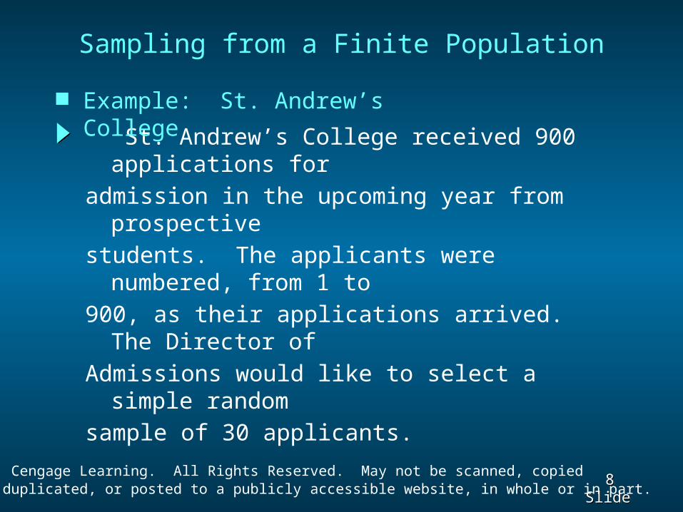
St. Andrew’s College received 900 applications for
admission in the upcoming year from prospective
students. The applicants were numbered, from 1 to
900, as their applications arrived. The Director of
Admissions would like to select a simple random
sample of 30 applicants.
Example: St. Andrew’s College
Sampling from a Finite Population
Page 9
9 9 Slide Slide© 2015 Cengage Learning. All Rights Reserved. May not be scanned, copied
or duplicated, or posted to a publicly accessible website, in whole or in part.
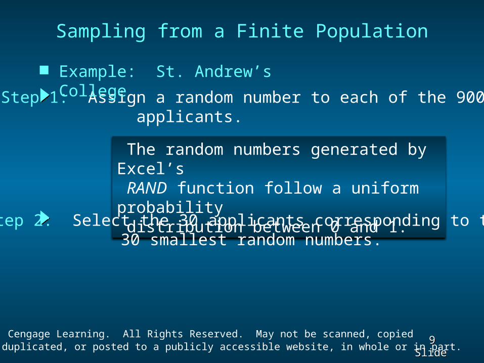
The random numbers generated by Excel’s RAND function follow a uniform probability distribution between 0 and 1.
Step 1: Assign a random number to each of the 900 applicants.
Step 2: Select the 30 applicants corresponding to the 30 smallest random numbers.
Sampling from a Finite Population
Example: St. Andrew’s College
Page 10
10 10 Slide Slide© 2015 Cengage Learning. All Rights Reserved. May not be scanned, copied
or duplicated, or posted to a publicly accessible website, in whole or in part.
Sampling from an Infinite Population
As a result, we cannot construct a frame for the population.
Sometimes we want to select a sample, but find it is not possible to obtain a list of all elements in the population.
Hence, we cannot use the random number selection procedure.
Most often this situation occurs in infinite population cases.
Page 11
11 11 Slide Slide© 2015 Cengage Learning. All Rights Reserved. May not be scanned, copied
or duplicated, or posted to a publicly accessible website, in whole or in part.
Populations are often generated by an ongoing process where there is no upper limit on the number of units that can be generated.
Sampling from an Infinite Population
Some examples of on-going processes, with infinite populations, are:
• parts being manufactured on a production line• transactions occurring at a bank
• telephone calls arriving at a technical help desk• customers entering a store
Page 12
12 12 Slide Slide© 2015 Cengage Learning. All Rights Reserved. May not be scanned, copied
or duplicated, or posted to a publicly accessible website, in whole or in part.
Sampling from an Infinite Population
A random sample from an infinite population is a sample selected such that the following conditions are satisfied.
• Each element selected comes from the population of interest.
In the case of an infinite population, we must select
a random sample in order to make valid statistical inferences about the population from which the sample is taken.
• Each element is selected independently.
Page 13
13 13 Slide Slide© 2015 Cengage Learning. All Rights Reserved. May not be scanned, copied
or duplicated, or posted to a publicly accessible website, in whole or in part.
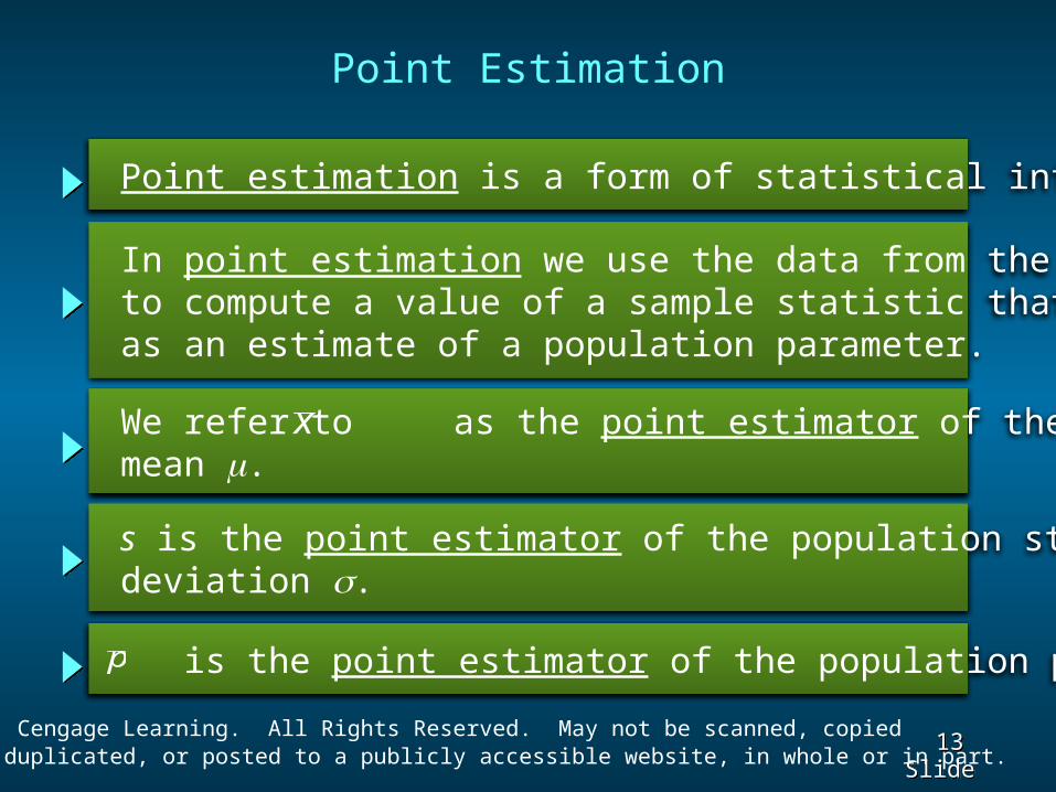
s is the point estimator of the population standard deviation .
In point estimation we use the data from the sample to compute a value of a sample statistic that serves as an estimate of a population parameter.
Point Estimation
We refer to as the point estimator of the population mean .
x
is the point estimator of the population proportion p.p
Point estimation is a form of statistical inference.
Page 14
14 14 Slide Slide© 2015 Cengage Learning. All Rights Reserved. May not be scanned, copied
or duplicated, or posted to a publicly accessible website, in whole or in part.
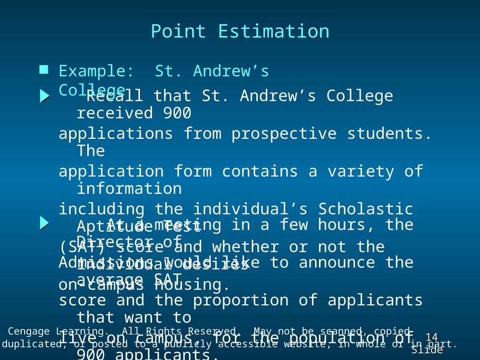
Recall that St. Andrew’s College received 900applications from prospective students. The application form contains a variety of
informationincluding the individual’s Scholastic Aptitude
Test (SAT) score and whether or not the individual
desireson-campus housing.
Example: St. Andrew’s College
Point Estimation
At a meeting in a few hours, the Director ofAdmissions would like to announce the average
SATscore and the proportion of applicants that
want tolive on campus, for the population of 900
applicants.
Page 15
15 15 Slide Slide© 2015 Cengage Learning. All Rights Reserved. May not be scanned, copied
or duplicated, or posted to a publicly accessible website, in whole or in part.
Point Estimation
Example: St. Andrew’s College
However, the necessary data on the applicants have
not yet been entered in the college’s computerized
database. So, the Director decides to estimate the
values of the population parameters of interest based
on sample statistics. The sample of 30 applicants is
selected using computer-generated random numbers.
Page 16
16 16 Slide Slide© 2015 Cengage Learning. All Rights Reserved. May not be scanned, copied
or duplicated, or posted to a publicly accessible website, in whole or in part.
as Point Estimator of x
as Point Estimator of pp
50,5201684
30 30ix
x
2( ) 210,51285.2
29 29ix x
s
20 30 .67p
Point Estimation
Note: Different random numbers would haveidentified a different sample which would haveresulted in different point estimates.
s as Point Estimator of
Page 17
17 17 Slide Slide© 2015 Cengage Learning. All Rights Reserved. May not be scanned, copied
or duplicated, or posted to a publicly accessible website, in whole or in part.
1697900
ix
2( )87.4
900ix
648.72
900p
Population Mean SAT Score
Population Standard Deviation for SAT Score
Population Proportion Wanting On-Campus Housing
Once all the data for the 900 applicants were entered
in the college’s database, the values of the population
parameters of interest were calculated.
Point Estimation
Page 18
18 18 Slide Slide© 2015 Cengage Learning. All Rights Reserved. May not be scanned, copied
or duplicated, or posted to a publicly accessible website, in whole or in part.
PopulationParameter
PointEstimator
PointEstimate
ParameterValue
m = Population mean SAT score
1697 1684
s = Population std. deviation for SAT score
87.4 s = Sample stan- dard deviation for SAT score
85.2
p = Population pro- portion wanting campus housing
.72 .67
Summary of Point EstimatesObtained from a Simple Random Sample
= Sample mean SAT score x
= Sample pro- portion wanting campus housing
p
Page 19
19 19 Slide Slide© 2015 Cengage Learning. All Rights Reserved. May not be scanned, copied
or duplicated, or posted to a publicly accessible website, in whole or in part.
Practical Advice
The target population is the population we want to make inferences about.
Whenever a sample is used to make inferences about a population, we should make sure that the targeted population and the sampled population are in close agreement.
The sampled population is the population from which the sample is actually taken.
Page 20
20 20 Slide Slide© 2015 Cengage Learning. All Rights Reserved. May not be scanned, copied
or duplicated, or posted to a publicly accessible website, in whole or in part.
Process of Statistical Inference
The value of is used tomake inferences about
the value of m.
x The sample data provide a value for
the sample mean .x
A simple random sampleof n elements is selected
from the population.
Population with mean
m = ?
Sampling Distribution of x
Page 21
21 21 Slide Slide© 2015 Cengage Learning. All Rights Reserved. May not be scanned, copied
or duplicated, or posted to a publicly accessible website, in whole or in part.
The sampling distribution of is the probabilitydistribution of all possible values of the sample mean .
x
x
Sampling Distribution of x
where: = the population mean
E( ) = x
x• Expected Value of
When the expected value of the point estimatorequals the population parameter, we say the pointestimator is unbiased.
Page 22
22 22 Slide Slide© 2015 Cengage Learning. All Rights Reserved. May not be scanned, copied
or duplicated, or posted to a publicly accessible website, in whole or in part.
Sampling Distribution of x
We will use the following notation to define thestandard deviation of the sampling distribution of
.x
s = the standard deviation of x x
s = the standard deviation of the population
n = the sample size
N = the population size
x• Standard Deviation of
Page 23
23 23 Slide Slide© 2015 Cengage Learning. All Rights Reserved. May not be scanned, copied
or duplicated, or posted to a publicly accessible website, in whole or in part.
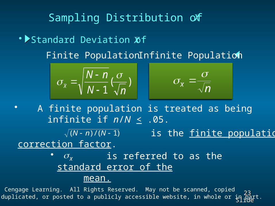
Sampling Distribution of x
Finite Population Infinite Population
)(1 nN
nNx
x n
• is referred to as the standard error of the
mean.
x
• A finite population is treated as being infinite if n/N < .05.• is the finite population correction factor.
( ) / ( )N n N 1
x• Standard Deviation of
Page 24
24 24 Slide Slide© 2015 Cengage Learning. All Rights Reserved. May not be scanned, copied
or duplicated, or posted to a publicly accessible website, in whole or in part.
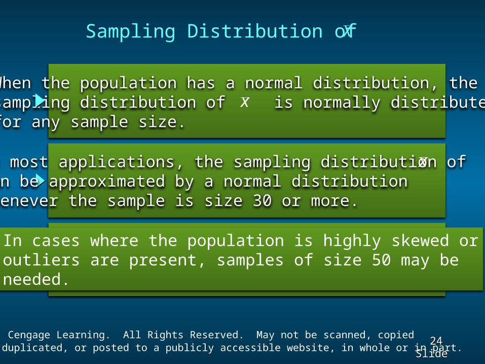
When the population has a normal distribution, thesampling distribution of is normally distributedfor any sample size.
x
In cases where the population is highly skewed oroutliers are present, samples of size 50 may beneeded.
In most applications, the sampling distribution of can be approximated by a normal distributionwhenever the sample is size 30 or more.
x
Sampling Distribution of x
Page 25
25 25 Slide Slide© 2015 Cengage Learning. All Rights Reserved. May not be scanned, copied
or duplicated, or posted to a publicly accessible website, in whole or in part.
Sampling Distribution of x
The sampling distribution of can be used toprovide probability information about how closethe sample mean is to the population mean m .
x
x
Page 26
26 26 Slide Slide© 2015 Cengage Learning. All Rights Reserved. May not be scanned, copied
or duplicated, or posted to a publicly accessible website, in whole or in part.
Central Limit Theorem
When the population from which we are selecting a random sample does not have a normal distribution,the central limit theorem is helpful in identifying theshape of the sampling distribution of . x
CENTRAL LIMIT THEOREM In selecting random samples of size n from apopulation, the sampling distribution of the sample mean can be approximated by a normal distribution as the sample size becomes large.
x
Page 27
27 27 Slide Slide© 2015 Cengage Learning. All Rights Reserved. May not be scanned, copied
or duplicated, or posted to a publicly accessible website, in whole or in part.
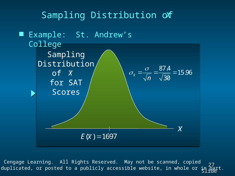
87.415.96
30x
n
( ) 1697E x x
SamplingDistribution
of for SATScores
x
Example: St. Andrew’s College
Sampling Distribution of x
Page 28
28 28 Slide Slide© 2015 Cengage Learning. All Rights Reserved. May not be scanned, copied
or duplicated, or posted to a publicly accessible website, in whole or in part.
What is the probability that a simple randomsample of 30 applicants will provide an estimate ofthe population mean SAT score that is within +/-10of the actual population mean ?
Example: St. Andrew’s College
Sampling Distribution of x
In other words, what is the probability that willbe between 1687 and 1707?
x
Page 29
29 29 Slide Slide© 2015 Cengage Learning. All Rights Reserved. May not be scanned, copied
or duplicated, or posted to a publicly accessible website, in whole or in part.
Step 1: Calculate the z-value at the upper endpoint of the interval.
z = (1707 - 1697)/15.96= .63
P(z < .63) = .7357
Step 2: Find the area under the curve to the left of the upper endpoint.
Sampling Distribution of x
Example: St. Andrew’s College
Page 30
30 30 Slide Slide© 2015 Cengage Learning. All Rights Reserved. May not be scanned, copied
or duplicated, or posted to a publicly accessible website, in whole or in part.
z .00 .01 .02 .03 .04 .05 .06 .07 .08 .09
. . . . . . . . . . .
.5 .6915 .6950 .6985 .7019 .7054 .7088 .7123 .7157 .7190 .7224
.6 .7257 .7291 .7324 .7357 .7389 .7422 .7454 .7486 .7517 .7549
.7 .7580 .7611 .7642 .7673 .7704 .7734 .7764 .7794 .7823 .7852
.8 .7881 .7910 .7939 .7967 .7995 .8023 .8051 .8078 .8106 .8133
.9 .8159 .8186 .8212 .8238 .8264 .8289 .8315 .8340 .8365 .8389. . . . . . . . . . .
Cumulative Probabilities for the Standard Normal
Distribution
Sampling Distribution of x
Example: St. Andrew’s College
Page 31
31 31 Slide Slide© 2015 Cengage Learning. All Rights Reserved. May not be scanned, copied
or duplicated, or posted to a publicly accessible website, in whole or in part.
x1697
15.96x
1707
Area = .7357
Sampling Distribution of x
Example: St. Andrew’s College
SamplingDistribution
of for SATScores
x
Page 32
32 32 Slide Slide© 2015 Cengage Learning. All Rights Reserved. May not be scanned, copied
or duplicated, or posted to a publicly accessible website, in whole or in part.
Step 3: Calculate the z-value at the lower endpoint of the interval.
Step 4: Find the area under the curve to the left of the lower endpoint.
z = (1687 - 1697)/15.96= - .63
P(z < -.63) = .2643
Sampling Distribution of x
Example: St. Andrew’s College
Page 33
33 33 Slide Slide© 2015 Cengage Learning. All Rights Reserved. May not be scanned, copied
or duplicated, or posted to a publicly accessible website, in whole or in part.
Sampling Distribution of for SAT Scoresx
x1687 1697
Area = .2643
15.96x
Example: St. Andrew’s College
SamplingDistribution
of for SATScores
x
Page 34
34 34 Slide Slide© 2015 Cengage Learning. All Rights Reserved. May not be scanned, copied
or duplicated, or posted to a publicly accessible website, in whole or in part.
Sampling Distribution of for SAT Scoresx
Step 5: Calculate the area under the curve between the lower and upper endpoints of the interval.
P(-.68 < z < .68) = P(z < .68) - P(z < -.68)= .7357 - .2643= .4714
The probability that the sample mean SAT score willbe between 1687 and 1707 is:
P(1687 < < 1707) = .4714x
Example: St. Andrew’s College
Page 35
35 35 Slide Slide© 2015 Cengage Learning. All Rights Reserved. May not be scanned, copied
or duplicated, or posted to a publicly accessible website, in whole or in part.
x170716871697
Sampling Distribution of for SAT Scoresx
Area = .4714
15.96x
Example: St. Andrew’s College
SamplingDistribution
of for SATScores
x
Page 36
36 36 Slide Slide© 2015 Cengage Learning. All Rights Reserved. May not be scanned, copied
or duplicated, or posted to a publicly accessible website, in whole or in part.
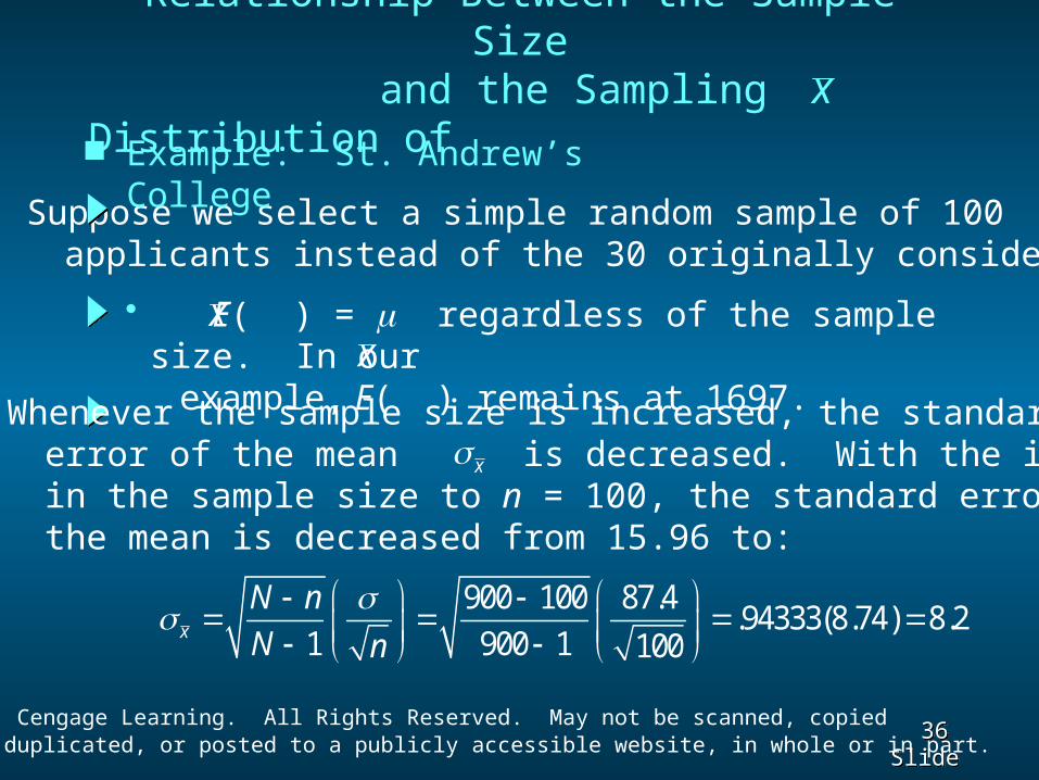
Relationship Between the Sample Size and the Sampling Distribution of x
• Suppose we select a simple random sample of 100 applicants instead of the 30 originally considered.
• E( ) = m regardless of the sample size. In our
example, E( ) remains at 1697.
xx
• Whenever the sample size is increased, the standard error of the mean is decreased. With the increase in the sample size to n = 100, the standard error of the mean is decreased from 15.96 to:
x
Example: St. Andrew’s College
900 100 87.4.94333(8.74) 8.2
1 900 1 100x
N nN n
Page 37
37 37 Slide Slide© 2015 Cengage Learning. All Rights Reserved. May not be scanned, copied
or duplicated, or posted to a publicly accessible website, in whole or in part.
Relationship Between the Sample Size and the Sampling Distribution of x
( ) 1697E x x
15.96x With n = 30,
8.2x With n = 100,
Example: St. Andrew’s College
Page 38
38 38 Slide Slide© 2015 Cengage Learning. All Rights Reserved. May not be scanned, copied
or duplicated, or posted to a publicly accessible website, in whole or in part.
• Recall that when n = 30, P(1687 < < 1707) = .4714.x
Relationship Between the Sample Size and the Sampling Distribution of x
• We follow the same steps to solve for P(1687 < < 1707) when n = 100 as we showed earlier when n = 30.
x
• Now, with n = 100, P(1687 < < 1707) = .7776.x• Because the sampling distribution with n = 100 has a smaller standard error, the values of have less variability and tend to be closer to the population mean than the values of with n = 30.
x
x
Example: St. Andrew’s College
Page 39
39 39 Slide Slide© 2015 Cengage Learning. All Rights Reserved. May not be scanned, copied
or duplicated, or posted to a publicly accessible website, in whole or in part.
Relationship Between the Sample Size and the Sampling Distribution of x
x170716871697
Area = .7776
8.2x
Example: St. Andrew’s College
SamplingDistribution
of for SATScores
x
Page 40
40 40 Slide Slide© 2015 Cengage Learning. All Rights Reserved. May not be scanned, copied
or duplicated, or posted to a publicly accessible website, in whole or in part.
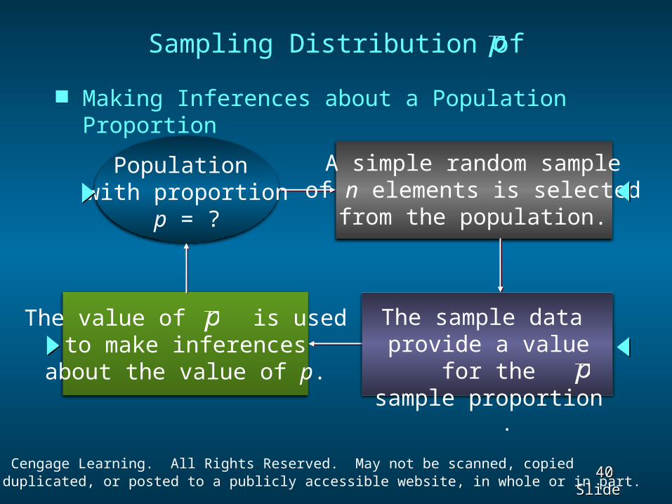
A simple random sampleof n elements is selected
from the population.
Population with proportion
p = ?
Making Inferences about a Population Proportion
The sample data provide a value for
thesample
proportion .
p
The value of is usedto make inferences
about the value of p.
p
Sampling Distribution ofp
Page 41
41 41 Slide Slide© 2015 Cengage Learning. All Rights Reserved. May not be scanned, copied
or duplicated, or posted to a publicly accessible website, in whole or in part.
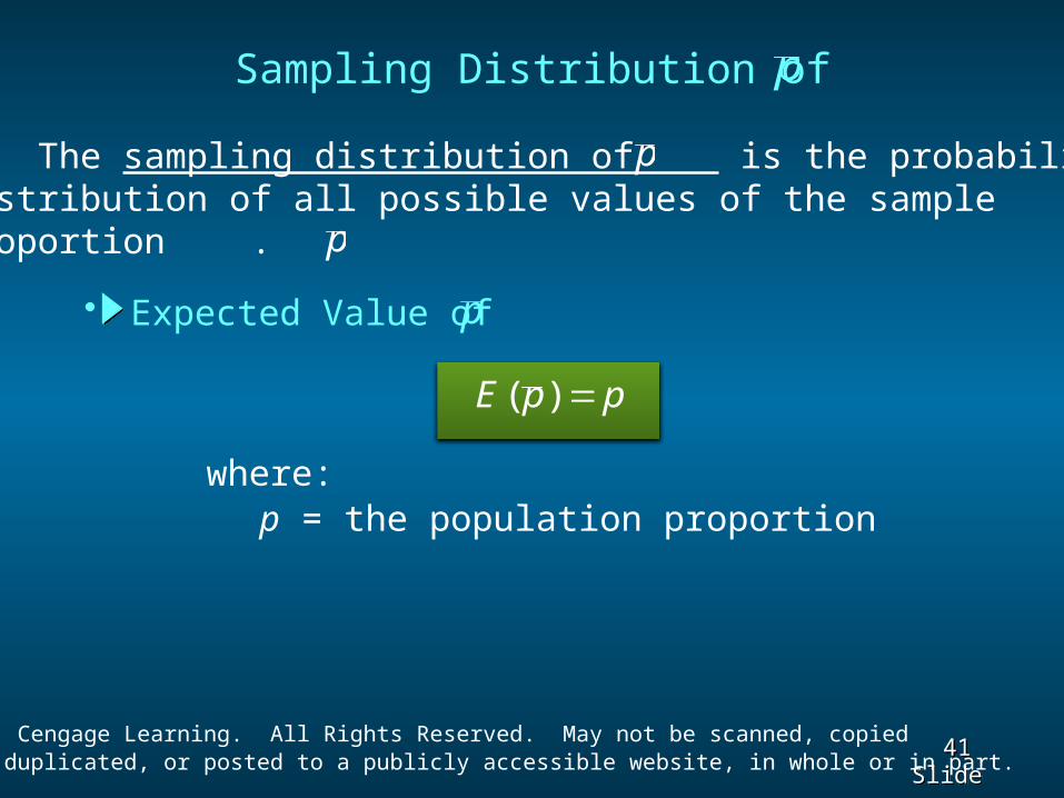
E p p( )
Sampling Distribution ofp
where:p = the population proportion
The sampling distribution of is the probabilitydistribution of all possible values of the sampleproportion .p
p
p• Expected Value of
Page 42
42 42 Slide Slide© 2015 Cengage Learning. All Rights Reserved. May not be scanned, copied
or duplicated, or posted to a publicly accessible website, in whole or in part.
n
pp
N
nNp
)1(
1
pp pn
( )1
• is referred to as the standard error of
the proportion.
p
Sampling Distribution ofp
Finite Population Infinite Population
p• Standard Deviation of
• is the finite population correction factor.
( ) / ( )N n N 1
Page 43
43 43 Slide Slide© 2015 Cengage Learning. All Rights Reserved. May not be scanned, copied
or duplicated, or posted to a publicly accessible website, in whole or in part.
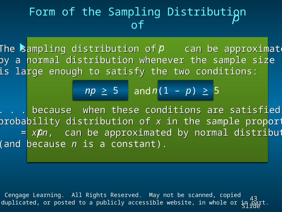
Form of the Sampling Distribution ofp
The sampling distribution of can be approximated by a normal distribution whenever the sample size is large enough to satisfy the two conditions:
. . . because when these conditions are satisfied, the probability distribution of x in the sample proportion, = x/n, can be approximated by normal distribution (and because n is a constant).
p
np > 5 n(1 – p) > 5and
p
Page 44
44 44 Slide Slide© 2015 Cengage Learning. All Rights Reserved. May not be scanned, copied
or duplicated, or posted to a publicly accessible website, in whole or in part.
Recall that 72% of the prospective students applying
to St. Andrew’s College desire on-campus housing.
Example: St. Andrew’s College
Sampling Distribution ofp
What is the probability that a simple random sample
of 30 applicants will provide an estimate of the
population proportion of applicant desiring on-campus
housing that is within plus or minus .05 of the actual
population proportion?
Page 45
45 45 Slide Slide© 2015 Cengage Learning. All Rights Reserved. May not be scanned, copied
or duplicated, or posted to a publicly accessible website, in whole or in part.
For our example, with n = 30 and p = .72, the
normal distribution is an acceptable approximation
because:
n(1 - p) = 30(.28) = 8.4 > 5
and
np = 30(.72) = 21.6 > 5
Sampling Distribution ofp
Example: St. Andrew’s College
Page 46
46 46 Slide Slide© 2015 Cengage Learning. All Rights Reserved. May not be scanned, copied
or duplicated, or posted to a publicly accessible website, in whole or in part.
p
.72(1 .72).082
30
( ) .72E p p
SamplingDistribution
of p
Sampling Distribution ofp
Example: St. Andrew’s College
Page 47
47 47 Slide Slide© 2015 Cengage Learning. All Rights Reserved. May not be scanned, copied
or duplicated, or posted to a publicly accessible website, in whole or in part.
Step 1: Calculate the z-value at the upper endpoint of the interval.
z = (.77 - .72)/.082 = .61
P(z < .61) = .7291
Step 2: Find the area under the curve to the left of the upper endpoint.
Sampling Distribution ofp
Example: St. Andrew’s College
Page 48
48 48 Slide Slide© 2015 Cengage Learning. All Rights Reserved. May not be scanned, copied
or duplicated, or posted to a publicly accessible website, in whole or in part.
z .00 .01 .02 .03 .04 .05 .06 .07 .08 .09
. . . . . . . . . . .
.5 .6915 .6950 .6985 .7019 .7054 .7088 .7123 .7157 .7190 .7224
.6 .7257 .7291 .7324 .7357 .7389 .7422 .7454 .7486 .7517 .7549
.7 .7580 .7611 .7642 .7673 .7704 .7734 .7764 .7794 .7823 .7852
.8 .7881 .7910 .7939 .7967 .7995 .8023 .8051 .8078 .8106 .8133
.9 .8159 .8186 .8212 .8238 .8264 .8289 .8315 .8340 .8365 .8389. . . . . . . . . . .
Cumulative Probabilities for the Standard Normal
Distribution
Sampling Distribution ofp
Example: St. Andrew’s College
Page 49
49 49 Slide Slide© 2015 Cengage Learning. All Rights Reserved. May not be scanned, copied
or duplicated, or posted to a publicly accessible website, in whole or in part.
.77.72
Area = .7291
p
SamplingDistribution
of p
.082p
Sampling Distribution ofp
Example: St. Andrew’s College
Page 50
50 50 Slide Slide© 2015 Cengage Learning. All Rights Reserved. May not be scanned, copied
or duplicated, or posted to a publicly accessible website, in whole or in part.
Step 3: Calculate the z-value at the lower endpoint of the interval.
Step 4: Find the area under the curve to the left of the lower endpoint.
z = (.67 - .72)/.082 = - .61
P(z < -.61) = .2709
Sampling Distribution ofp
Example: St. Andrew’s College
Page 51
51 51 Slide Slide© 2015 Cengage Learning. All Rights Reserved. May not be scanned, copied
or duplicated, or posted to a publicly accessible website, in whole or in part.
.67 .72
Area = .2709
p
SamplingDistribution
of p
.082p
Sampling Distribution ofp
Example: St. Andrew’s College
Page 52
52 52 Slide Slide© 2015 Cengage Learning. All Rights Reserved. May not be scanned, copied
or duplicated, or posted to a publicly accessible website, in whole or in part.
P(.67 < < .77) = .4582p
Step 5: Calculate the area under the curve between the lower and upper endpoints of the interval.
P(-.61 < z < .61) = P(z < .61) - P(z < -.61)= .7291 - .2709= .4582
The probability that the sample proportion of applicantswanting on-campus housing will be within +/-.05 of theactual population proportion :
Sampling Distribution ofp
Example: St. Andrew’s College
Page 53
53 53 Slide Slide© 2015 Cengage Learning. All Rights Reserved. May not be scanned, copied
or duplicated, or posted to a publicly accessible website, in whole or in part.
.77.67 .72
Area = .4582
p
SamplingDistribution
of p
.082p
Sampling Distribution ofp
Example: St. Andrew’s College
Page 54
54 54 Slide Slide© 2015 Cengage Learning. All Rights Reserved. May not be scanned, copied
or duplicated, or posted to a publicly accessible website, in whole or in part.
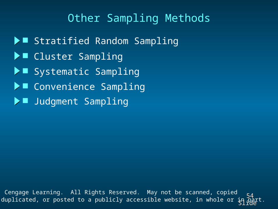
Other Sampling Methods
Stratified Random Sampling Cluster Sampling Systematic Sampling Convenience Sampling Judgment Sampling
Page 55
55 55 Slide Slide© 2015 Cengage Learning. All Rights Reserved. May not be scanned, copied
or duplicated, or posted to a publicly accessible website, in whole or in part.
The population is first divided into groups of elements called strata.
Stratified Random Sampling
Each element in the population belongs to one and only one stratum.
Best results are obtained when the elements within each stratum are as much alike as possible (i.e. a homogeneous group).
Page 56
56 56 Slide Slide© 2015 Cengage Learning. All Rights Reserved. May not be scanned, copied
or duplicated, or posted to a publicly accessible website, in whole or in part.
Stratified Random Sampling
A simple random sample is taken from each stratum.
Formulas are available for combining the stratum sample results into one population parameter estimate.
Advantage: If strata are homogeneous, this method is as “precise” as simple random sampling but with a smaller total sample size.
Example: The basis for forming the strata might be department, location, age, industry type, and so on.
Page 57
57 57 Slide Slide© 2015 Cengage Learning. All Rights Reserved. May not be scanned, copied
or duplicated, or posted to a publicly accessible website, in whole or in part.
Cluster Sampling
The population is first divided into separate groups of elements called clusters.
Ideally, each cluster is a representative small-scale version of the population (i.e. heterogeneous group).
A simple random sample of the clusters is then taken.
All elements within each sampled (chosen) cluster form the sample.
Page 58
58 58 Slide Slide© 2015 Cengage Learning. All Rights Reserved. May not be scanned, copied
or duplicated, or posted to a publicly accessible website, in whole or in part.
Cluster Sampling
Advantage: The close proximity of elements can be cost effective (i.e. many sample observations can be obtained in a short time).
Disadvantage: This method generally requires a larger total sample size than simple or stratified random sampling.
Example: A primary application is area sampling, where clusters are city blocks or other well-defined areas.
Page 59
59 59 Slide Slide© 2015 Cengage Learning. All Rights Reserved. May not be scanned, copied
or duplicated, or posted to a publicly accessible website, in whole or in part.
Systematic Sampling
If a sample size of n is desired from a population containing N elements, we might sample one element for every n/N elements in the population.
We randomly select one of the first n/N elements from the population list.
We then select every n/Nth element that follows in the population list.
Page 60
60 60 Slide Slide© 2015 Cengage Learning. All Rights Reserved. May not be scanned, copied
or duplicated, or posted to a publicly accessible website, in whole or in part.
Systematic Sampling
This method has the properties of a simple random sample, especially if the list of the population elements is a random ordering.
Advantage: The sample usually will be easier to identify than it would be if simple random sampling were used.
Example: Selecting every 100th listing in a telephone book after the first randomly selected listing
Page 61
61 61 Slide Slide© 2015 Cengage Learning. All Rights Reserved. May not be scanned, copied
or duplicated, or posted to a publicly accessible website, in whole or in part.
Convenience Sampling
It is a nonprobability sampling technique. Items are included in the sample without known probabilities of being selected.
Example: A professor conducting research might use student volunteers to constitute a sample.
The sample is identified primarily by convenience.
Page 62
62 62 Slide Slide© 2015 Cengage Learning. All Rights Reserved. May not be scanned, copied
or duplicated, or posted to a publicly accessible website, in whole or in part.
Advantage: Sample selection and data collection are relatively easy.
Disadvantage: It is impossible to determine how representative of the population the sample is.
Convenience Sampling
Page 63
63 63 Slide Slide© 2015 Cengage Learning. All Rights Reserved. May not be scanned, copied
or duplicated, or posted to a publicly accessible website, in whole or in part.
Judgment Sampling
The person most knowledgeable on the subject of the study selects elements of the population that he or she feels are most representative of the population.
It is a nonprobability sampling technique.
Example: A reporter might sample three or four senators, judging them as reflecting the general opinion of the senate.
Page 64
64 64 Slide Slide© 2015 Cengage Learning. All Rights Reserved. May not be scanned, copied
or duplicated, or posted to a publicly accessible website, in whole or in part.
Judgment Sampling
Advantage: It is a relatively easy way of selecting a sample.
Disadvantage: The quality of the sample results depends on the judgment of the person selecting the sample.
Page 65
65 65 Slide Slide© 2015 Cengage Learning. All Rights Reserved. May not be scanned, copied
or duplicated, or posted to a publicly accessible website, in whole or in part.
Recommendation
It is recommended that probability sampling methods (simple random, stratified, cluster, or systematic) be used.
For these methods, formulas are available for evaluating the “goodness” of the sample results in terms of the closeness of the results to the population parameters being estimated.
An evaluation of the goodness cannot be made with non-probability (convenience or judgment) sampling methods.
Page 66
66 66 Slide Slide© 2015 Cengage Learning. All Rights Reserved. May not be scanned, copied
or duplicated, or posted to a publicly accessible website, in whole or in part.
End of Chapter 7