Arthur CHARPENTIER, Advanced Econometrics Graduate Course, Winter 2017, Université de Rennes 1
Motivation
Before computers, statistical analysis used probability theory to derive statisticalexpression for standard errors (or confidence intervals) and testing procedures,for some linear model
yi = xTi β + εi = β0 +
p∑j=1
βjxj,i + εi.
But most formulas are approximations, based on large samples (n→∞).
With computers, simulations and resampling methods can be used to produce(numerical) standard errors and testing procedure (without the use of formulas,but with a simple algorithm).
@freakonometrics 2
Arthur CHARPENTIER, Advanced Econometrics Graduate Course, Winter 2017, Université de Rennes 1
Overview
Linear Regression Model: yi = β0 + xTi β + εi = β0 + β1x1,i + β2x2,i + εi
• Asymptotics vs. Finite Distance : boostrap techniques
• Penalization : Parcimony, Complexity and Overfit
• From least squares to other regressions : quantiles, expectiles, etc.
@freakonometrics 3
Arthur CHARPENTIER, Advanced Econometrics Graduate Course, Winter 2017, Université de Rennes 1
Historical References
Permutation methods go back to Fisher (1935) The Design of Experiments andPitman (1937) Significance tests which may be applied to samples from anypopulation
(there are n! distinct permutations)
Jackknife was introduced in Quenouille (1949) Approximate tests of correlation intime series, popularized by Tukey (1958) Bias and confidence in not quite largesamples
Bootstrapping started with Monte Carlo algorithms in the 40’s, see e.g. Simon &Burstein (1969) Basic Research Methods in Social Science
Efron (1979) Bootstrap methods: Another look at the jackknife defined aresampling procedure that was coined as “bootstrap”.
(there are nn possible distinct ordered bootstrap samples)
Arthur CHARPENTIER, Advanced Econometrics Graduate Course, Winter 2017, Université de Rennes 1
Bootstrap Techniques (in one slide)
Bootstrapping is an asymptotic refinementbased on computer based simulations.Underlying properties: we know when itmight work, or notIdea : {(yi,xi)} is obtained from a stochas-tic model under PWe want to generate other samples (notmore observations) to reduce uncertainty.
@freakonometrics 6
Arthur CHARPENTIER, Advanced Econometrics Graduate Course, Winter 2017, Université de Rennes 1
Heuristic Intuition for a Simple (Financial) Model
Consider a return stochastic model, rt = µ+ σεt, for t = 1, 2, · · · , T , with (εt) isi.id. N (0, 1) [Constant Expected Return Model, CER]
µ = 1T
T∑t=1
rt and σ2 = 1T
T∑t=1
[rt − µ
]2then (standard errors)
se[µ] = σ√T
and se[σ] = σ√2T
then (confidence intervals)
µ ∈[µ± 2se[µ]
]and σ ∈
[σ ± 2se[σ]
]What if the quantity of interest, θ, is another quantity, e.g. a Value-at-Risk ?
@freakonometrics 7
Arthur CHARPENTIER, Advanced Econometrics Graduate Course, Winter 2017, Université de Rennes 1
Heuristic Intuition for a Simple (Financial) Model
One can use nonparametric bootstrap
1. resampling: generate B “bootstrap samples” by resampling with replacementin the original data,
r(b) = {r(b)1 , · · · , r(b)
T }, with r(b)t ∈ {r1, · · · , rT }.
2. For each sample r(b), compute θ(b)
3. Derive the empirical distribution of θ from{θ(1), · · · , θ(B)}.
4. Compute any quantity of interest, standard error, quantiles, etc.
E.g. estimate the bias
bias[θ] = 1B
B∑b=1
θ(b)
︸ ︷︷ ︸bootstrap mean
− 1B
B∑b=1
θ︸ ︷︷ ︸estimate
@freakonometrics 8
Arthur CHARPENTIER, Advanced Econometrics Graduate Course, Winter 2017, Université de Rennes 1
Heuristic Intuition for a Simple (Financial) Model
E.g. estimate the standard error
se[θ] =
√√√√ 1B − 1
B∑b=1
(θ(b) − 1
B
B∑b=1
θ(b)
)2
E.g. estimate the confidence interval, if the bootstrap distribution looks Gaussian
θ ∈[θ ± 2se[θ]
]and if the distribution does not look Gaussian
θ ∈[q
(B)α/2; q(B)
1−α/2
]where q(B)
α denote a quantile from{θ(1), · · · , θ(B)}.
@freakonometrics 9
Arthur CHARPENTIER, Advanced Econometrics Graduate Course, Winter 2017, Université de Rennes 1
Monte Carlo Techniques in Statistics
Law of large numbers (---), if E[X] = 0 and Var[X] = 1 :√n Xn
L→ N (0, 1)
What if n is small? What is the distribution of Xn?
Example : X such that 2− 12 (X − 1) ∼ χ2(1)
Use Monte Carlo Simulation to derive confidence in-tervall for Xn (—).Generate samples {x(m)
1 , · · · , x(m)n } from χ2(1), and
compute x(m)n
Then estimate the density of {x(1)n , · · · , x(m)
n }, quan-tiles, etc.
−0.5 0.0 0.5
0.0
0.5
1.0
1.5
Problem : need to know the true distribution of X.
What if we have only {x1, · · · , xn} ?
Generate samples {x(m)1 , · · · , x(m)
n } from Fn, and compute x(m)n (—)
@freakonometrics 10
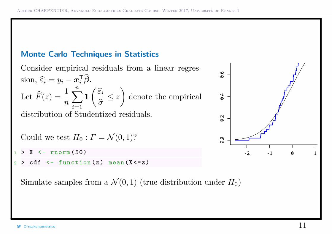
Arthur CHARPENTIER, Advanced Econometrics Graduate Course, Winter 2017, Université de Rennes 1
Monte Carlo Techniques in StatisticsConsider empirical residuals from a linear regres-sion, εi = yi − xT
i β.
Let F (z) = 1n
n∑i=1
1(εiσ≤ z)
denote the empirical
distribution of Studentized residuals.
Could we test H0 : F = N (0, 1)?
1 > X <- rnorm (50)
2 > cdf <- function (z) mean(X <=z)
Simulate samples from a N (0, 1) (true distribution under H0)
@freakonometrics 11
Arthur CHARPENTIER, Advanced Econometrics Graduate Course, Winter 2017, Université de Rennes 1
Quantifying Bias
Consider X with mean µ = E(X). Let θ = exp[µ], then θ = exp[x] is a biasedestimator of θ, see Horowitz (1998) The Bostrap
Idea 1 : Delta Method, i.e. if√n[τn − τ ] L−→N (0, σ2), then, if g′(τ) exists and is
• instrumental variables and two-stage least squares
@freakonometrics 17
Arthur CHARPENTIER, Advanced Econometrics Graduate Course, Winter 2017, Université de Rennes 1
Monte Carlo Techniques to Compute Integrals
Monte Carlo is a very general technique, that can be used to compute anyintegral.
Let X ∼ Cauchy what is P[X > 2]. Observe that
P[X > 2] =∫ ∞
2
dx
π(1 + x2) (∼ 0.15)
since f(x) = 1π(1 + x2) and Q(u) = F−1(u) = tan
(π[u− 1
2]).
Crude Monte Carlo: use the law of large numbers
p1 = 1n
n∑i=1
1(Q(ui) > 2)
where ui are obtained from i.id. U([0, 1]) variables.
Observe that Var[p1] ∼ 0.127n .
@freakonometrics 18
Arthur CHARPENTIER, Advanced Econometrics Graduate Course, Winter 2017, Université de Rennes 1
Crude Monte Carlo (with symmetry): P[X > 2] = P[|X| > 2]/2 and use the lawof large numbers
p2 = 12n
n∑i=1
1(|Q(ui)| > 2)
where ui are obtained from i.id. U([0, 1]) variables.
Observe that Var[p2] ∼ 0.052n .
Using integral symmetries :∫ ∞2
dx
π(1 + x2) = 12 −
∫ 2
0
dx
π(1 + x2)
where the later integral is E[h(2U)] where h(x) = 2π(1 + x2) .
From the law of large numbers
p3 = 12 −
1n
n∑i=1
h(2ui)
@freakonometrics 19
Arthur CHARPENTIER, Advanced Econometrics Graduate Course, Winter 2017, Université de Rennes 1
where ui are obtained from i.id. U([0, 1]) variables.
Observe that Var[p3] ∼ 0.0285n .
Using integral transformations :∫ ∞2
dx
π(1 + x2) =∫ 1/2
0
y−2dy
π(1− y−2)
which is E[h(U/2)] where h(x) = 12π(1 + x2) .
From the law of large numbers
p4 = 14n
n∑i=1
h(ui/2)
where ui are obtained from i.id. U([0, 1]) variables.Observe that Var[p4] ∼ 0.0009
n .
@freakonometrics 20
Arthur CHARPENTIER, Advanced Econometrics Graduate Course, Winter 2017, Université de Rennes 1
Simulation in Econometric Models
(almost) all quantities of interest can be writen T (ε) with ε ∼ F .
E.g. β = β + (XTX)−1XTε
We need E[T (ε)] =∫t(ε)dF (ε)
Use simulations, i.e. draw n values {ε1, · · · , εn} since
E
[1n
n∑i=1
T (εi)]
= E[T (ε)] (unbiased)
1n
n∑i=1
T (εi)L→ E[T (ε)] as n→∞ (consistent)
@freakonometrics 21
Arthur CHARPENTIER, Advanced Econometrics Graduate Course, Winter 2017, Université de Rennes 1
Generating (Parametric) Distributions
Inverse cdf Technique :
Let U ∼ U([0, 1]), then X = F−1(U) ∼ F .
Proof 1:
P[F−1(U) ≤ x] = P[F ◦ F−1(U) ≤ F (x)] = P[U ≤ F (x)] = F (x)
Proof 2: set u = F (x) or x = F−1(u) (change of variable)
E[h(X)] =∫Rh(x)dF ?(x) =
∫ 1
0h(F−1(u))du = E[h(F−1(U))]
with U ∼ U([0, 1]), i.e. X L= F−1(U).
@freakonometrics 22
Arthur CHARPENTIER, Advanced Econometrics Graduate Course, Winter 2017, Université de Rennes 1
Rejection Techniques
Problem : If X ∼ F , how to draw from X?, i.e. X conditional on X ∈ [a, b] ?
Solution : draw X and use accept-reject method
1. if x ∈ [a, b], keep it (accept)2. if x 6∈ [a, b], draw another value (reject)If we generate n values, we accept - on average -[F (b)− F (a)] · n draws.
@freakonometrics 23
Arthur CHARPENTIER, Advanced Econometrics Graduate Course, Winter 2017, Université de Rennes 1
Importance SamplingProblem : If X ∼ F , how to draw from X condi-tional on X ∈ [a, b] ?Solution : rewrite the integral and use importancesampling methodThe conditional censored distribution X? is
dF ?(x) = dF (x)F (b)− F (a)1(x ∈ [a, b])
Alternative for truncated distributions : let U ∼U([0, 1]) and set U = [1 − U ]F (a) + UF (b) andY = F−1(U)
@freakonometrics 24
Arthur CHARPENTIER, Advanced Econometrics Graduate Course, Winter 2017, Université de Rennes 1
Going Further : MCMC
Intuition : we want to use the Central Limit Theorem, but i.id. sample is a (too)strong assumtion: if (Xi) is i.id. with distribution F ,
1√n
(n∑i=1
h(Xi)−∫h(x)dF (x)
)L→ N (0, σ2), as n→∞.
Use the ergodic theorem: if (Xi) is a Markov Chain with invariant measure µ,
1√n
(n∑i=1
h(Xi)−∫h(x)dµ(x)
)L→ N (0, σ2), as n→∞.
See Gibbs sampler
Example : complicated joint distribution, but simple conditional ones
@freakonometrics 25
Arthur CHARPENTIER, Advanced Econometrics Graduate Course, Winter 2017, Université de Rennes 1
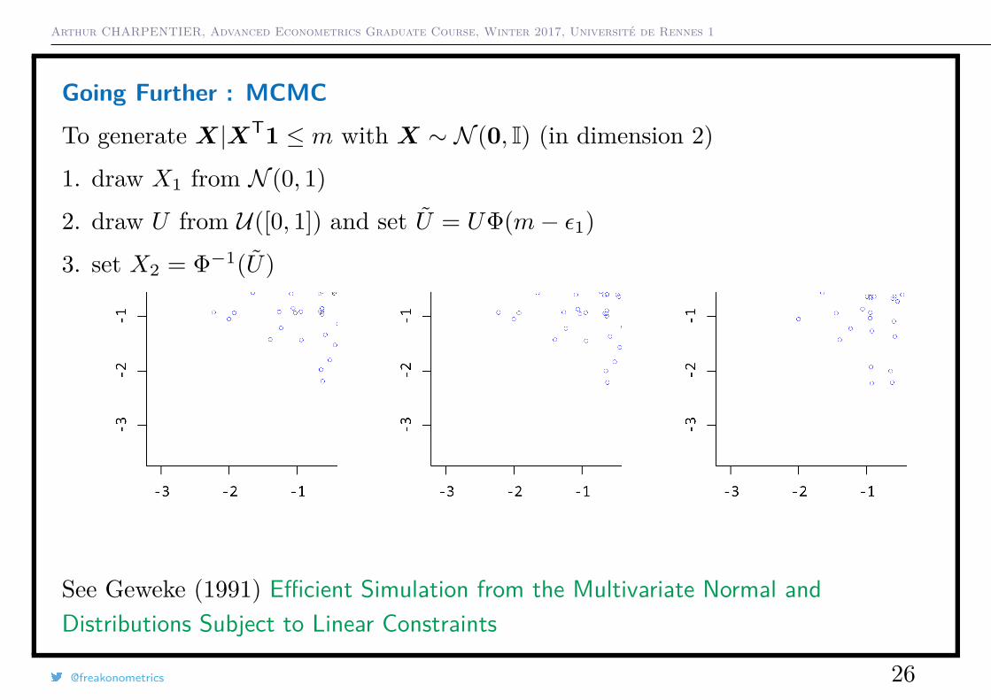
Going Further : MCMC
To generate X|XT1 ≤ m with X ∼ N (0, I) (in dimension 2)
1. draw X1 from N (0, 1)
2. draw U from U([0, 1]) and set U = UΦ(m− ε1)
3. set X2 = Φ−1(U)
See Geweke (1991) Efficient Simulation from the Multivariate Normal andDistributions Subject to Linear Constraints
Arthur CHARPENTIER, Advanced Econometrics Graduate Course, Winter 2017, Université de Rennes 1
Monte Carlo Techniques in Statistics
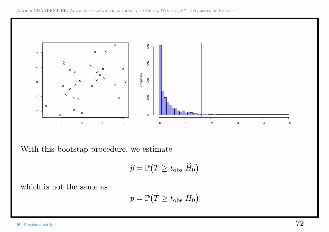
Let {y1, · · · , yn} denote a sample from a collection of n i.id. random variableswith true (unknown) distribution F0. This distribution can be approximated byFn.
parametric model : F0 ∈ F = {Fθ; θ ∈ Θ}.
nonparametric model : F0 ∈ F = {F is a c.d.f.}
The statistic of interest is Tn = Tn(y1, · · · , yn) (see e.g. Tn = βj).
Let Gn denote the statistics of Tn:
Exact distribution : Gn(t, F0) = PF (Tn ≤ t) under F0
We want to estimate Gn(·, F0) to get confidence intervals, i.e. α-quantiles
G−1n (α, F0) = inf
{t;Gn(t, F0) ≥ α
}or p-values,
p = 1−Gn(tn, F0)
@freakonometrics 27
Arthur CHARPENTIER, Advanced Econometrics Graduate Course, Winter 2017, Université de Rennes 1
Approximation of Gn(tn, F0)
Two strategies to approximate Gn(tn, F0) :
1. Use G∞(·, F0), the asymptotic distribution as n→∞.
2. Use G∞(·, Fn)
Here Fn can be the empirical cdf (nonparametric bootstrap) or Fθ(parametric
bootstrap).
@freakonometrics 28
Arthur CHARPENTIER, Advanced Econometrics Graduate Course, Winter 2017, Université de Rennes 1
Approximation of Gn(tn, F0): Linear Model
Consider the test of H0 : βj = 0, p-value being p = 1−Gn(tn, F0)
• Linear Model with Normal Errors yi = xTi β + εi with εi ∼ N (0, σ2).
Then (βj − βj)2
σ2j
∼ F(1, n− k) = Gn(·, F0) where F0 is N (0, σ2)
• Linear Model with Non-Normal Errors yi = xTi β + εi, with E[εi] = 0.
Then (βj − βj)2
σ2j
L→ ξ2(1) = G∞(·, F0) as n→∞.
@freakonometrics 29
Arthur CHARPENTIER, Advanced Econometrics Graduate Course, Winter 2017, Université de Rennes 1
Approximation of Gn(tn, F0): Linear Model
Application yi = xTi β + εi, ε ∼ N (0, 1), ε ∼ U([−1,+1]) or ε ∼ Std(ν = 2).
One can define Jackknife bias and Jackknife variance
b? = −1n
n∑i=1
`?i and v? = 1n(n− 1)
(n∑i=1
`?2i − nb?2)
cf numerical differentiation when ε = − 1(n− 1) .
@freakonometrics 64
Arthur CHARPENTIER, Advanced Econometrics Graduate Course, Winter 2017, Université de Rennes 1
Convergence
Given a sample {y1, · · · , yn}, i.id. with distribution F , set
Fn(t) = 1n
n∑i=1
1(yi ≤ t)
Thensup
{|Fn(t)− F0(t)|
} P→ 0, as n→∞.
@freakonometrics 65
Arthur CHARPENTIER, Advanced Econometrics Graduate Course, Winter 2017, Université de Rennes 1
How many Boostrap Samples?
Easy to take B ≥ 5000
R > 100 to estimate bias or variance
R > 1000 to estimate quantiles
Bias Variance Quantile
0 500 1000 1500 2000
−0.
15−
0.10
−0.
050.
000.
050.
100.
15
Nb Boostrap Sample
Bia
s
0 500 1000 1500 2000
0.10
0.15
0.20
0.25
Nb Boostrap Sample
Var
ianc
e
0 500 1000 1500 2000
4.50
4.55
4.60
4.65
4.70
Nb Boostrap Sample
Qua
ntile
@freakonometrics 66
Arthur CHARPENTIER, Advanced Econometrics Graduate Course, Winter 2017, Université de Rennes 1
Consistency
We expect something like
Gn(t, Fn) ∼ G∞(t, Fn) ∼ G∞(t, F0) ∼ Gn(t, F0)
Gn(t, Fn) is said to be consistent if under each F0 ∈ F ,
supt∈ R
{|Gn(t, Fn)−G∞(t, F0)|
} P→ 0
Example: let θ = EF0(X) and consider Tn =√n(X − θ). Here
Gn(t, F0) = PF0(Tn ≤ t)
Based on boostrap samples, a bootstrap version of Tn is
T (b)n =
√n(X
(b) −X)since X = E
Fn(X)
and Gn(t, Fn) = PFn
(Tn ≤ t)
@freakonometrics 67
Arthur CHARPENTIER, Advanced Econometrics Graduate Course, Winter 2017, Université de Rennes 1
Consistency
Consider a regression model yi = xTi β + εi
The natural assumption is E[εi|X] = 0 with εi’s i.id.∼ F .
The parameter of interest is θ = βj , and let βj = θ(Fn).
1. The statistics of interest is Tn =√n[βj − βj
].
We want to know Gn(t, F0) = PF0(Tn ≤ t).
Let x(b) denote a bootsrap sample.
Compute T (b)n =
√n(β
(b)j − βj
), and then
Gn(t, Fn) = 1B
B∑b=1
1(T (b)n ≤ t)
@freakonometrics 68
Arthur CHARPENTIER, Advanced Econometrics Graduate Course, Winter 2017, Université de Rennes 1
Consistency
2. The statistics of interest is Tn =√n
[βj − βj
]√Var[βj ]
.
We want to know Gn(t, F0) = PF0(Tn ≤ t).
Let x(b) denote a bootsrap sample.
Compute T (b)n =
√n
[β
(b)j − βj
]√Var(b)[βj ]
, and then
Gn(t, Fn) = 1B
B∑b=1
1(T (b)n ≤ t)
This second option is more accurate than the first one :
@freakonometrics 69
Arthur CHARPENTIER, Advanced Econometrics Graduate Course, Winter 2017, Université de Rennes 1
Consistency
The approximation error of bootstrap applied to asymptotically pivotal statisticis smaller than the approximation error of bootstrap applied on asymptoticallynon-pivotal statistic, see Horowitz (1998) The Bostrap.
Here, asymptotically pivotal means that
G∞(t, F ) = G∞(t), ∀F ∈ F .
Assume now that the quantity of interest is θ = Var[β].
Consider a bootstrap procedure, then one can prove that