IEEE TRANSACTIONS ON INDUSTRIAL ELECTRONICS, VOL. 40, NO. 1, FEBRUARY 1993 23 Sliding Mode Control Design Principles and Applications to Electric Drives Vadim I. Utkin Abstract-The paper deals with the basic concepts, mathemat- ics, and design aspects of variable structure systems as well as sliding modes as a principle operation mode. The main argu- ments in favor of sliding mode control are order reduction, decoupling design procedure, disturbance rejection, insensitivity to parameter variations, and simple implementation by means of power converters. The control algorithms and data processing used in variable structure systems are analyzed. The potential of sliding mode control methodology is demonstrated for versatility of electric drives and functional goals of control. I. INTRODUCTION high level of scientific and publication activity, an All nremitting interest in variable structure control en- hanced by effective applications to automation problems most diverse in their physical nature, and functional pur- poses are a cogent argument to consider this class of nonlinear systems as a prospective area for study and applications. The term “variable structure system” (VSS) first made its appearance in the late 1950’s. Since that time, the first expectations of such systems have naturally been reevalu- ated, their real potential has been revealed, new research directions have been originated due to the appearance of new classes of control problems, new mathematical meth- ods, recent advances in switching circuitry, and (as a consequence) new control principles. The paper is oriented to base-stone ideas of VSS design methods and selected set of applications rather than the survey information or a historical sequence of the events accompanying VSS development since at its different stages survey papers on theory [1]-[4] and applications [51, 161 have been published. In addition, monographs [7]-[12] summarize the results of these stages. Furthermore, it will be shown that the dominant role in VSS theory is played by sliding modes, and the core idea of designing VSS control algorithms consists of enforcing this type of motion in some manifolds in system state spaces. Implementation of sliding mode control implies high-frequency switching. It does not cause any difficulties when electric drives are controlled since the “on-off” operation mode is the only admissible one for power Manuscript received June 6, 1992. A revised version of the paper was presented at the IEEE VARSCON ’91 Workshop, Reno, NV, June 6, 1991. The author is with the Institute of Control Sciences, 117 806, Moscow, Russia. IEEE Log Number 9204071. converters. This reason predetermined both the high ef- ficiency of sliding mode control for electric drives and the author choice of the application selection topic in this paper. 11. SLIDING MODES IN VSS Variable structure systems consist of a set of continu- ous subsystems with a proper switching logic and, as a result, control actions are discontinuous functions of sys- tem state, disturbances (if they are accessible for mea- surement), and reference inputs. In the course of the entire history of control theory, intensity of discontinuous control systems investigation has been maintained at a high enough level. In particular, at the first stage, on-off or bang-bang regulators are ranked highly due to ease of implementation and efficiency of control hardware. Futhermore, we shall deal with the variable structure systems governed by X =f(x,t,u), x E Rn,U E R” u+(x, t) if s(x) > 0 (for each component) u-(x,t) if s(x) < 0 (1) The VSS (1) with continuous functions f, s, U+, U- con- sists of 2” subsystems and its structure varies on m surfaces at the state space. From the point of view of our later treatment, it is worth quoting the elementary exam- ple of a second-order system with bang-bang control and sliding mode: x + a2X + a,x = U, U = -M signs s = cx + X, M , c , a , , a2 - const (2) which was considered by Andronov et al. [131 in connec- tion with his study of autopilot dynamics. It follows from analysis of the (X, x) state plane (Fig. 1) that, in the neighborhood of segment mn on the switching line s = 0, the trajectories run in opposite directions, which leads to the appearance of a sliding mode along this line. The switching line equation s = 0 may be treated as a motion 0278-0046/93$03.00 0 1993 IEEE
Transcript
IEEE TRANSACTIONS ON INDUSTRIAL ELECTRONICS, VOL. 40, NO. 1, FEBRUARY 1993 23
Sliding Mode Control Design Principles and Applications to Electric Drives
Vadim I. Utkin
Abstract-The paper deals with the basic concepts, mathemat- ics, and design aspects of variable structure systems as well as sliding modes as a principle operation mode. The main argu- ments in favor of sliding mode control are order reduction, decoupling design procedure, disturbance rejection, insensitivity to parameter variations, and simple implementation by means of power converters. The control algorithms and data processing used in variable structure systems are analyzed. The potential of sliding mode control methodology is demonstrated for versatility of electric drives and functional goals of control.
I. INTRODUCTION
high level of scientific and publication activity, an All nremitting interest in variable structure control en- hanced by effective applications to automation problems most diverse in their physical nature, and functional pur- poses are a cogent argument to consider this class of nonlinear systems as a prospective area for study and applications.
The term “variable structure system” (VSS) first made its appearance in the late 1950’s. Since that time, the first expectations of such systems have naturally been reevalu- ated, their real potential has been revealed, new research directions have been originated due to the appearance of new classes of control problems, new mathematical meth- ods, recent advances in switching circuitry, and (as a consequence) new control principles.
The paper is oriented to base-stone ideas of VSS design methods and selected set of applications rather than the survey information or a historical sequence of the events accompanying VSS development since at its different stages survey papers on theory [1]-[4] and applications [51, 161 have been published. In addition, monographs [7]-[12] summarize the results of these stages.
Furthermore, it will be shown that the dominant role in VSS theory is played by sliding modes, and the core idea of designing VSS control algorithms consists of enforcing this type of motion in some manifolds in system state spaces. Implementation of sliding mode control implies high-frequency switching. It does not cause any difficulties when electric drives are controlled since the “on-off” operation mode is the only admissible one for power
Manuscript received June 6, 1992. A revised version of the paper was presented at the IEEE VARSCON ’91 Workshop, Reno, NV, June 6, 1991.
The author is with the Institute of Control Sciences, 117 806, Moscow, Russia.
IEEE Log Number 9204071.
converters. This reason predetermined both the high ef- ficiency of sliding mode control for electric drives and the author choice of the application selection topic in this paper.
11. SLIDING MODES IN VSS Variable structure systems consist of a set of continu-
ous subsystems with a proper switching logic and, as a result, control actions are discontinuous functions of sys- tem state, disturbances (if they are accessible for mea- surement), and reference inputs. In the course of the entire history of control theory, intensity of discontinuous control systems investigation has been maintained at a high enough level. In particular, at the first stage, on-off or bang-bang regulators are ranked highly due to ease of implementation and efficiency of control hardware.
Futhermore, we shall deal with the variable structure systems governed by
X = f ( x , t , u ) , x E Rn,U E R”
u + ( x , t ) if s ( x ) > 0 (for each component) u - ( x , t ) if s ( x ) < 0
(1)
The VSS (1) with continuous functions f, s, U + , U - con- sists of 2” subsystems and its structure varies on m surfaces at the state space. From the point of view of our later treatment, it is worth quoting the elementary exam- ple of a second-order system with bang-bang control and sliding mode:
x + a2X + a , x = U ,
U = -M signs
s = cx + X, M , c , a , , a2 - const ( 2 )
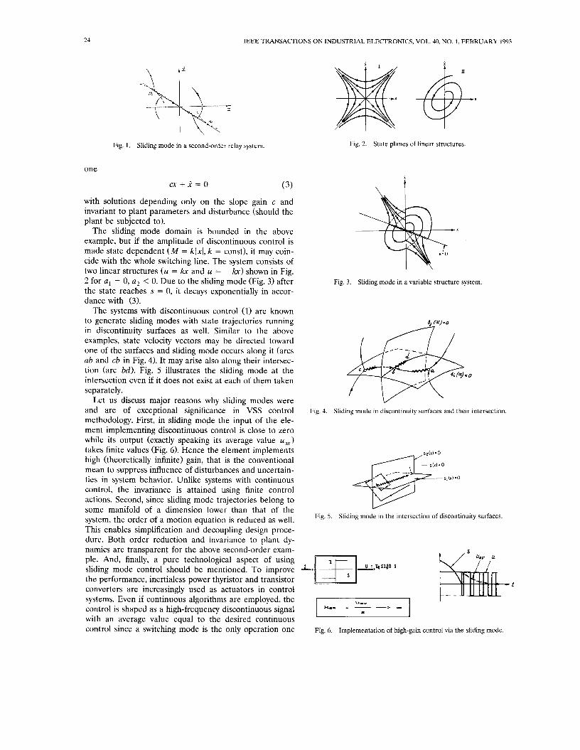
which was considered by Andronov et al. [131 in connec- tion with his study of autopilot dynamics. It follows from analysis of the (X, x) state plane (Fig. 1) that, in the neighborhood of segment mn on the switching line s = 0, the trajectories run in opposite directions, which leads to the appearance of a sliding mode along this line. The switching line equation s = 0 may be treated as a motion
0278-0046/93$03.00 0 1993 IEEE
24 IEEE TRANSACTIONS ON INDUSTRIAL ELECTRONICS, VOL. 40, NO. 1, FEBRUARY 1993
Fig. 1. Sliding mode in a second-order relay system.
one
c x + x = o
Fig. 2. State planes of linear structures.
(3) \ i with solutions depending only on the slope gain c and invariant to plant parameters and disturbance (should the plant be subjected to).
The sliding mode domain is bounded in the above example, but if the amplitude of discontinuous control is made state dependent ( M = klxl, k = const), it may coin- cide with the whole switching line. The system consists of two linear structures (U = krc and U = -la) shown in Fig. 2 for a, = 0, a2 < 0. Due to the sliding mode (Fig. 3) after the state reaches s = 0, it decays exponentially in accor- dance with (3).
The systems with discontinuous control (1) are known to generate sliding modes with state trajectories running in discontinuity surfaces as well. Similar to the above examples, state velocity vectors may be directed toward one of the surfaces and sliding mode occurs along it (arcs ab and cb in Fig. 4). It may arise also along their intersec- tion (arc bd). Fig. 5 illustrates the sliding mode at the intersection even if it does not exist at each of them taken separately.
Let us discuss major reasons why sliding modes were and are of exceptional significance in VSS control methodology. First, in sliding mode the input of the ele- ment implementing discontinuous control is close to zero while its output (exactly speaking its average value U,) takes finite values (Fig. 6). Hence the element implements high (theoretically infinite) gain, that is the conventional mean to suppress influence of disturbances and uncertain- ties in system behavior. Unlike systems with continuous control, the invariance is attained using finite control actions. Second, since sliding mode trajectories belong to some manifold of a dimension lower than that of the system, the order of a motion equation is reduced as well. This enables simplification and decoupling design proce- dure. Both order reduction and invariance to plant dy- namics are transparent for the above second-order exam- ple. And, finally, a pure technological aspect of using sliding mode control should be mentioned. To improve the performance, inertialess power thyristor and transistor converters are increasingly used as actuators in control systems. Even if continuous algorithms are employed, the control is shaped as a high-frequency discontinuous signal with an average value equal to the desired continuous control since a switching mode is the only operation one
x
Fig. 3. Sliding mode in a variable structure system.
Fig. 4. Sliding mode in discontinuity surfaces and their intersection.
Fig. 5. Sliding mode in the intersection of discontinuity surfaces.
f
Fig. 6. Implementation of high-gain control via the sliding mode.
UTKIN: SLIDING MODE CONTROL DESIGN PRINCIPLES
, M
t I 0 n
0
- 9 U a t i 0
25
E x I. s t c n c V
c 0
n &
1 S L X D X N a M O D E CONTROL I M a t h c - m a t I c a 1 Methods
Applications 1 1
m 0
t 0
P T? 0 C
e a a - = i n
i n d U = t
I r l
n
I. 0
Fig. 7. Scope of sliding mode control theory.
for the converters. It seems more natural to employ the algorithms oriented toward discontinuous control actions.
The study of sliding modes is a multifacet problem that embrances mathematical, control theoretical, and applica- tion aspects. The chapters and sections of this study are shown in Fig. 7.
111. MATHEMATICAL METHODS To justify strictly the arguments in favor of employing
multidimensional sliding modes we need mathematical methods of describing sliding modes in the intersection of discontinuity surfaces s = 0 and the conditions for this motion to exist.
The first problem arises due to discontinuity of control since the relevant differential equations do not satisfy conventional theorems on existence uniqueness solutions. We confine ourselves to a second-order example to demonstrate that discontinuous control systems may need subtle treatment. Let the discontinuous control in the system
X I = o.3X2 -k uxI
i , = - 0 . 7 ~ ~ + 4u3x,, U = -sign xis, s = x1 + x2 be implemented by a limiter and then by a hysteresis relay element so that A-the width of the limiter linear zone and the hysteresis loop-is small enough when compared with the magnitude of control. The experiment with A =
0.01 shows that in spite of closeness of the controls, the motion along the switching line is unstable in the first case and asymptotically stable in the second one (Fig. 8).
Fig. 8. Ambiguity of sliding mode equations.
In cases when conventional methods are not applicable, the usual approach is to employ the regularization ap- proach or replacing the initial problem by a closely similar one, for which familiar methods can be used. In particu- lar, taking into account delay or hysteresis of a switching element, small time constants neglected in an ideal model, replacing a discontinuous function by continuous approxi- mation, are the examples of regularization since disconti- nuity points (if they exist) are isolated.
In our opinion, the universal approach to regularization consists of introducing a boundary layer llsll < A around manifold s = 0 where an ideal discontinuous control is replaced by a real one such that the state trajectories of system (1) are not confined to this manifold but run arbitrarily inside the layer (Fig. 9). The only assumption for this motion is that the solution exists in ordinary sense. If, with the width of the boundary layer tending to zero, the limit of this solution exists, it is taken as a
26 IEEE TRANSACTIONS ON INDUSTRIAL ELECTRONICS, VOL. 40, NO. 1 , FEBRUARY 1993
Fig. 9. Boundary layer regularization.
solution to the system with ideal sliding modes. Otherwise we have to recognize that the equations beyond disconti- nuity surfaces do not derive unambiguously the motion equation in their intersection.
Boundary-layer regularization enables substantiation of the so-called equicalent control method [ 141 intended for deriving a sliding mode equation in the systems depending on linear control:
X = f ( x , t ) + B ( x , t ) u (4)
where B ( x , t ) is an n x m matrix. In accordance with the method control, U should be replaced by the equivalent control, which is the solution to
S = Cf + GBu,, = 0, G = ( a s / a x )
For det GB # 0 (ue! = - (GB)- 'Gf ) , the sliding mode equation in the manifold s = 0 is
i = [ I - B(GB)-'G]f. ( 5 )
Since s ( x ) = 0 in sliding mode m components of the state vector x may be found as a function of the rest ( n - m) ones: x 2 = so(x,), x2 ,so E R", x , E R"-'" and, corre- spondingly, the order of the sliding motion equation may be reduced by m:
The idea of the equivalent control method may be easily explained with the help of geometric consideration. Slid- ing mode trajectories lie in the manifold s = 0 and the equivalent control ueq being a solution to the equation S = 0 implies replacing discontinuous control by such a continuous one that the state velocity vector lies in the tangential manifold.
Uniqueness of sliding mode equations explains why the study of control systems with linear dependence on con- trol has turned out the main (if not the only) stream in VSS theory. Note that in the above second-order example, nonlinear dependence of the motion equation on control resulted in the ambiguous sliding mode equations.
The second mathematical problem relates to conditions for a sliding mode to exist. They are equivalent to condi- tions of state trajectory convergence to the intersection of discontinuity surfaces s = 0. Therefore, the existence con- ditions may be formulated in terms of stability of the origin in m-dimensional space s, or subspace of the dis- tances to discontinuity surfaces. To derive existence con- ditions in analytical form, the equation of the projection of overall motion on subspace s
S = Gf + GBu (7)
should be analyzed for example by designing a Lyapunov function. The simplest case is for GB being an identity matrix. Then for U = - M signs ((signs)T = (signsl;.., signs,)) with M exceeding the upper estimates of vector Gf elements, the functions S, and s, ( i = 1;",m) have different signs. It means that the sliding mode will occur in each discontinuity surface.
The most interesting fact is that the Lyapunov function testifying to convergence to the manifold s = 0 is a finite function of time. It vanishes after a finite time interval. AS a result, sliding mode arises in a finite time instant in contrast to continuous systems with only asymptotic tend- ing to any manifold consisting of system trajectories [ 111.
IV. DESIGN PROCEDURE The discussed methods pertaining to sliding mode
equations and existence conditions constitute the back-
UTKIN: SLIDING MODE CONTROL DESIGN PRINCIPLES 27
ground for the variety of design procedures in VSS. De- coupling or invariance or both are inherent in any of them. High dimension and uncertainties in system behav- ior are known to be serious obstacles in applying efficient control algorithms and using both analytical and computa- tional methods.
In connection with control of high-dimensional plants, the design methods permitting decoupling of the overall motion into independent partial components are of great interest. Decoupling in discontinuous control systems (4) is easily feasible. The sliding mode equation (6) is of a reduced order, does not depend on control, and does depend on the discontinuity surface equation. The design procedure consists of two stages. At stage 1, the function s,, is handled as a control in (6) and designed in accor- dance with some performance criterion-a standard con- trol task. In stage 2 selection of discontinuous control follows to switching logic in (1) to enforce the sliding mode, which is equivalent to stability task in s space (7) of a reduced order as well. It should be noted that the last problem is not very difficult since its dimension and that of control coincide. As a result, the control design is decoupled into two independent tasks of lower dimen- sions: ( n - m)th order at the first stage and mth order at the second. In a thus-designed system starting from some finite time instant, the motion with the prescribed proper- ties will arise.
Time interval preceding the sliding mode decreases with the growth of control magnitude i l l ] , and if it is small enough it is the very sliding equations that predeter- mine control system properties.
What shall we expect of sliding modes in systems oper- ating under uncertainty conditions? Suppose that in the system equation
i = f ( x , t ) + B ( x , t ) u + h ( x , t ) (8)
vector h(x, t ) represents all the factors whose influence on the control process should be eliminated. If for each x and t
h E range { B ) (9)
which means that disturbances act in control space, then there exists control U , such that Bu, = -h and hence the system is invariant to h(x,t). But control U,, would hardly be implementable since the disturbances may be inaccessible for measurement.
As we had established the sliding mode equation in any manifold does not depend on control. Similarly, via the equivalent control method, it can be shown that sliding mode is independent on h(x, t ) as well, therefore condi- tion (9) is the invariance condition for sliding mode con- trol. It is important that for the design of an invariant system there is no need to measure vector h. To ensure sliding mode existence, only an upper estimate of h (a number or function) is needed.
v. SLIDING MODE CONTROL 1N LINEAR SYSTEMS
Consider conventional control tasks for linear plants i =Rx + B u , x E Rn,U E R"
( A , B are constant matrices, rank B = m) to demonstrate the sliding mode design procedure based on the decou- pling principle.
The system (10) may be transformed to the regular form [151
(10)
i , = A , , x , + A , ? X , i2 = A 2 , x , + A,?xz + B 2 u (11)
where A, , (i, j = 1,2), B, are constant matrices of rele- vant dimensions, x, E R"-"', x2 E R'", det B , # 0. As- suming that control vector components have discontinu- ities on linear surfaces,
s = cx, +I,, s E R"' ( 12) we find that, when the sliding mode appears on manifold s = 0 (i.e., x2 = -Cx,), the system behavior is governed by the ( n - m)th-order equation
i , = ( A , , - A & > x , . (13) One of the possible ways of obtaining the required
dynamic properties of the control systems is assigning eigenvalues of a closed-loop system with linear feedback. However, whereas in the context of initial system (10) we are concerned with a task of full dimensionality, introduc- ing a sliding mode reduces it, since the order of the sliding equation (13) is decreased by an amount equal to the control dimension. For controllable systems (lo), there always exists a matrix C, ensuring the desired eigenvalues of the system (13) [16]. The matrix C being a solution to the (n-m)th-order eigenvalue assigning task determines the equation of discontinuity surfaces (12). The second stage of the design procedure is choice of discontinuous control such that the sliding mode always arises at the manifold s = 0, which is equivalent to stability of the origin in m-dimensional space s. The motion projection on the s space is described by an equation similar to (7):
S = Rx + B,u , fi = (CA, , + A , I ) X , + (CA, , + A 2 2 ) X 2 .
U = -alxlB,' sign s, a - const
S = Rx - alxlsigns.
The discontinuous control
(1x1 is the sum of vector x component moduli) leads to
(14) There exists such positive value of a that the functions S, and s, ( i = l;.., m) have different signs. It means that the sliding mode will occur in each discontinuity surface.
Within the same framework a discontinuous control may be designed in accordance with a mean square crite- rion
I = ['kTQxdt, Q 2 0.
If we are concerned with optimization of sliding motions, then the sliding manifold should be linear while coeffi-
28 IEEE TRANSACTIONS ON INDUSTRIAL ELECTRONICS, VOL. 40, NO. 1, FEBRUARY 1993
cients of its equation are found from the Riccati equation of a reduced order similar to the above eigenvalue assign- ment [ l l ] . The control (14) fits to generate a sliding mode in manifold (12) with both constant and time-varying matrices C.
Invariance to disturbances and plant parameter varia- tion is one of the main problems of control theory. As mentioned in Section IV generating sliding modes results in invariance to all factors to be rejected acting in control subspace. For linear systems
i = A + Bu + D f ( t ) , f ( t ) E R'
this condition was formulated in terms of system and input matrices in [17]. The sliding mode in manifold (12) is invariant to the disturbance f ( t ) and the variations of the parameters AA( t ) ( A = A , , + AA(t), A,, = const) if D E range {B} , AA(t ) E range {B} , correspondingly. Simi- larly, the decoupling conditions in the interconnected systems may be found: interconnection matrices in each of the subsystems should belong to corresponding control subspace.
VI. THE CHA~TERING PROBLEM The subject of this section is of great importance when-
ever we intend to establish a bridge between the recom- mendations of the theory and applications. Bearing in mind that the control has a high-frequency component, we should analyze the robustness or the problem of corre- spondence between an ideal sliding mode and real-life processes at the presence of unmodeled dynamics. Ne- glected small time constants ( p l and p2 in Fig. 10) in plant models, sensors, and actuators leads to dynamic discrepancy (zl and z2 are the unmodeled-dynamics state vectors).
In accordance with the singular perturbation theory [ 181 in systems with continuous control, a fast component of the motion decays rapidly and a slow one depends on the small time constants continuously (Fig. 11).
In continuous control systems the solution depends on the small parameters continuously as well. But unlike continuous systems, the switchings in control excite the unmodeled dynamics, which leads to oscillations in the state vector at a finite frequency (Fig. 12). The oscilla- tions, usually referred to as chattering, are known to result in low control accuracy, high heat losses in electri- cal power circuits, and high wear of moving mechanical parts. These phenomena have been considered as serious obstacles for applications of sliding mode control in many papers and discussions. A recent study [19] and practical experience showed that the chattering caused by unmod- eled dynamics may be eliminated in systems with asymp- totic observers (Fig. 13). In spite of the presence of unmodeled dynamics, ideal sliding arises, it is described by a singularly perturbed differential equation with solutions free from a high-frequency component and close to those of the ideal system (Fig. 14). As shown in Fig. 13 an asymptotic observer serves as a bypass for a high-frequency
-, EL>DT, Fig. 10. Unmodeled dynamics of actuator and sensor.
Fig. 1 1 . System with continuous control.
t , L( t )
+> -1141n. m o a -
Fig. 12. Chattering in system with discontinuous control.
I I Aslmptotic observer
component, therefore the unmodeled dynamics is not excited. Preservation of sliding modes in systems with asymptotic observers predetermined successful applica- tions of the sliding mode control [61.
The alternative approach to handling dynamic discrep- ancies is a continuous approximation of discontinuous control [20]-[22]. It should be noted that too high a slope in the middle part of the approximation functions (Fig. 15) may result in excitation of the unmodeled dynamics as well, and the trade-off between accuracy and robustness must be achieved. In addition to that, continuous approxi- mation is nonadmissible for many applications where on-off operation is the "way of life" for actuators (e.g., thyristor or transistor conversions).
VII. CONTROL OF ELECTRIC DRIVES The experience that has been gained in the applications
of sliding mode algorithms testifies to their efficiency and versatility [6]. Control of electric drives is one of the most challenging applications due to wide use of electric ser- vomechanisms in control systems, the advances of high- speed switching circuitry, and insufficient linear control methodology for internally nonlinear high-order plants such as ac motors. Implementation of sliding modes by
UTKIN: SLIDING MODE CONTROL DESIGN PRINCIPLES
~
29
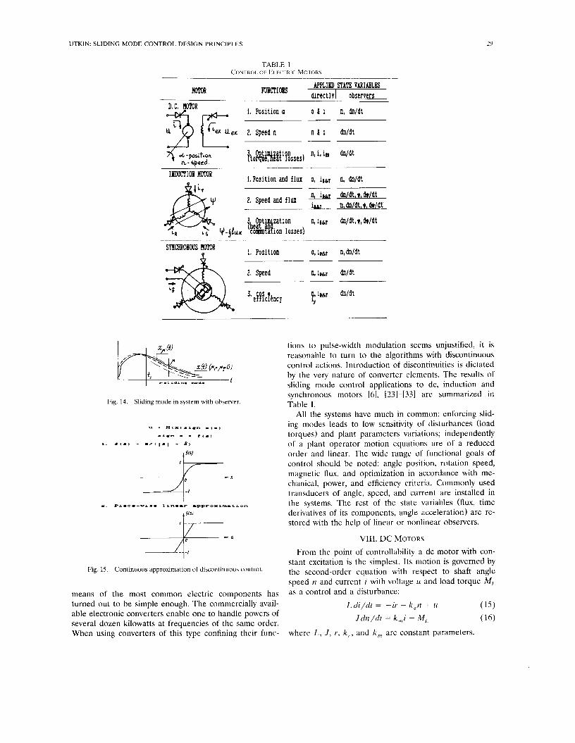
TABLE I CONTROL OF ELKI RIC MO I ORS
APPLIED STATE VARIABLB mCNoBs brectld observers
“)R
1. Posi t ion a a 6 i n, dn/dt
uex 2. Speed n n 6 1 dn/dt
__
LPos i t ion and f lux a, it,^^ n, dn/dt IgWCTIOB HOlVR
2, Speed and f lux
LR
1. Posi t ion a,iffil n,dn/dt
Fig. 14. Sliding mode in system with observer.
Fig. 15. Continuous approximation of discontinuous control.
means of the most common electric components has turned out to be simple enough. The commercially avail- able electronic converters enable one to handle powers of several dozen kilowatts at frequencies of the same order. When using converters of this type confining their func-
tions to pulse-width modulation seems unjustified, it is reasonable to turn to the algorithms with discontinuous control actions. Introduction of discontinuities is dictated by the very nature of converter elements. The results of sliding mode control applications to dc, induction and synchronous motors [6], [23]-[33] are summarized in Table I .
All the systems have much in common: enforcing slid- ing modes leads to low sensitivity of disturbances (load torques) and plant parameters variations; independently of a plant operator motion equations are of a reduced order and linear. The wide range of functional goals of control should be noted: angle position, rotation speed, magnetic flux, and optimization in accordance with me- chanical, power, and efficiency criteria. Commonly used transducers of angle, speed, and current are installed in the systems. The rest of the state variables (flux, time derivatives of its components, angle acceleration) are re- stored with the help of linear or nonlinear observers.
VIII. DC MOTORS From the point of controllability a dc motor with con-
stant excitation is the simplest. Its motion is governed by the second-order equation with respect to shaft angle speed n and current i with voltage U and load torque M L as a control and a disturbance:
L d i / d t = -ir - k e n + U
J d n / d t = k,,i - M , (15) ( 16)
where L , J, r , k , , and k,, are constant parameters.
30 IEEE TRANSACTIONS ON INDUSTRIAL ELECTRONICS, VOL. 40, NO. 1, FEBRUARY 1993
r ,. Jr 1,r A
U , > k , (n , - An) + -MI> + - iz , + - ( A n - A n ) krn k k m
Let n,(t) be a reference input, then the second-order motion equation with respect to the error x , = n,(t) - n is of form
.
where a,, a2, and b are positive parameters, f ( t ) -a time function depending on M,(t), n & t ) and their time deriva- tives.
For discontinuous control
u = U ( ) sign s, s = cxl + x 2 (18)
the error x , decays exponentially should the sliding mode occur on the line s = 0 since its equation
ul,, c - const
cxl + il = 0
is linear and does not depend on f ( t ) , As follows from
S = cx2 - a l x l - a2x , + f ( t ) - bu, sign s
in the system (17), (18) with
> 1~x2 - ~ 1 x 1 - ~ 2 x 2 + f ( t > I (19)
the values of s and S have opposite signs and the state reaches the sliding line s = 0 after a finite time interval. Inequality (19) determines the voltage needed for enforc- ing the sliding mode, as a result, the control error is steered to zero.
For implementation of control (181, angle acceleration is needed ( x 2 = ii, - iz). Under the assumptions that the angle speed n and the current i can be measrued directly and the load torque varies slowly or
dM,/dt = 0 (20)
a conventional Luenberger reduced-order observer may be designed:
dM/d t = 1/J( -1M + l’n + lk,i) (21)
with 1 - const, as an estimate of M = M , + In. Ac- cording to (161, (2!), and (21) the equation for the mis- match M = M - M is of the form
1 - d M / d t = - - M .
J
By a proper choic? of gain 1, the desired convergence rate of to zero or M - In to M , may be provided. It means that the load torque is known and the time derivative dn /d t may be found from (16).
Similarly, the sliding mode control may be designed for position and torque control with or without measurement of the motor current. In addition to control of mechanical coordinates, optimization in accordance with a power consumption criterion may be provided for dc motors with a controlled excitation current [6].
Section VI was dedicated to sliding mode control in the systems with unmodeled dynamics in which the partial
motion components may be separated by rates and then the fast one is neglected. A similar situation may happen when controlling a dc motor with a mechanical motion being much slower than an electromagnetic one. Formally it means that L a J in (15), (16), which may be presented as
di dt
L- = -ir - k,(n,, - A n ) + u (15‘)
d A n dt
J-- = -k,i + M , + Jiz,
with a control error An = no - n. Let us write down formally the equation for An making L be equal to zero. Then, substitution of the solution of (15’) with L = 0
1
r r ( n , - A n ) + -U
ke I = --
into (16‘) yields
Equation (23) is taken as a reduced-order model of a dc motor. Within the framework of the model (23), discontin- uous control U = uO sign An, depending only on the con- trol error (in contrast to (18), depending on its time derivative) for high enough U , , provides the sliding mode in “manifold” An = 0; and, as a result ideal tracking the reference input n,,(t) by the shaft rotation speed. How- ever, as it was discussed in Section VI, the unmodeled dynamics (15‘) may excite nonadmissible chattering. Fol- lowing the recommendation of Section VI, chattering may be eliminated by using asymptotic observers.
Bearing in mind that M , = 0, let us design an asymp- totic observer to estimate An (23) and M,:
d An k, ,k , krn J - = - ( n o - An) - -U
dt r r
+ M, + .hio + l , (An - A n ) (24)
dML
dt ~ = / , (An - A n )
where An and kL are estimates for An and M,, li and 1, are constant. Control is a discontinuous function of the error estimate
u = u0 sign A n . (26)
The values of A, and its time derivative (24) have differ- ent signs if
Origination of the sliding mode means that the discyntin- uous control (26), (27) reduces the error estimate An to zero. To derive a sliding mode equation in accordance
UTKIN: SLIDING MODE CONTROL DESIGN PRINCIPLES 31
with the equivalent control method (Sect. III), the solu- tion to dii /dt = 0 (24) with respect to control
should be substituted into system (15'), (16'), (25) for U :
d An dt
J - = -k,i + M L + Jl i , (29)
- = - 1 2 A n . ( 30) d k L
dt
Equations (281, (29), (3?), and ML = 0 describe the sliding mode in the manifold An = 0. According to the theory of singularly perturbed systems [18] for L 4 J , the fast mo- tion of the linear system may be neglected by zeroing the parameter L. Substitution of the solution to algebraic equation (28) ( L = 0) with respect to i jn to (29) results in a motion equation for A n and aL = ML - MI.:
JAri= - -An - kekm
r a - 1, An
ML = -1, An
Apparently the eigenvalues of the homogeneous system may be assigned at our will by a proper choice of 1, and 1, and the desired rate of the control error An decay may be guaranteed.
The principal advantage of the reduced-order-based method is that the angle acceleration is not needed for designing sliding mode control.
IX. INDUCTION MOTORS The most simple, reliable and economic of all
motors-maintenance-free induction motors-supersede dc motors in today's technology, although, in terms of controllability, induction motors seem the most compli- cated. Their behavior is described by a nonlinear high- order system of differential equations:
whtre n is a rotor angle velocity, and two-dimensional vectors 4T = (4a, 4p); iT = ( i , , i p ) , uT = ( u a , u p ) are ro- tor flux, stator curent, and voltage in the fixed coordinate system ( a , p) , respectively; M and M L are a torque developed by a motor and a load torque, u R , U , , U,-phase voltages, which may be made equal either to uo or -uo; eR , e,, e , are unit vectors of phase windings R, S, T ; and J , x H , xs , x R , rR, rs are motor parameters.
The control goal is to make one of the mechanical coordinates, for example, an angle speed n(t) , be equal to a reference input n o ( t ) and the magnitude of the rotor flux Il+(t>ll be equal to its scalar reference input 4,(t>. The deviations from the desired motions are described by the functions
and c,, c2 are const positive values. The static inverter forms three independent controls
u R , u s , u T , so one degree of freedom can be used to satisfy some additional criterion. Let the voltages uR, u s , uT constitute a three-phase balanced system, which means that the equality
should hold for any t . If all three functions s,, s2, s3 are equal to zero then, in
addition to balanced system condition (32), the speed and flux mismatches decay exponentially since s, = 0, s, = 0 with c1,c2 > 0 are first-order differential equations. This means that the design task is reduced to enforcing the sliding mode in the manifold s = 0, sT = (sl, s,, s3) in the system (31) with control uT = ( u R , us, U , ) . Projection of the system motion on subspace s can be written as
ds
dt dn 1 ' H . - = = + + U (33) - - ( M - M L ) , M =
dt J X R
- - - -4, - n4b + rR-z,
_ - - i p4 , ) where vector F = ( f l , f 2 , 0) and matrix D do not depend
'4a ' R x H . on control and are continuous functions of the motor dt x R X R state and inputs. Matrix D is of form
- r,i, + U , di, ' R ' H '4 , dt x , x R - X ; x R dt i-- _ - -
D = [:'I D , =
and
d = (1,1, l), k - const,det D f 0. - rsi, + up
dip _ -
32 IEEE TRANSACTIONS ON INDUSTRIAL ELECTRONICS, VOL. 40, NO. 1, FEBRUARY 1993
Discontinuous control will be designed using the Lya- punov function
U = 0 . 5 ~ ~ ~ 2 0.
Find its time derivative on the state trajectories of system (33):
du/dt = sT( F + Du) . (34)
Substitution of control
U = - U g sign s * , s* = DTs
( s * f = (s;,s;,s;)
into (34) yields
du/dt = ( s * ) ~ F * - uoIs*I
where
The conditions
U g > Ifi*l, i = 1 , 2 , 3 (35)
provide negativeness of du/dt and hence the origin in the space s* (and by virtue of det D f 0 in the space s as well) is asymptotically stable. Hence sliding mode arises in the manifold s = 0, which enables one to steer the vari- ables under control to the desired values. Note that the existence condition (35) are inequalities, therefore the only range of parameter variations and a load torque should be known for the choice of necessary values of phase voltages.
The equation of discontinuity surfaces s* = 0 depend on an angle acceleration, rotor flux, and its time deriva- tive. These values may be found using asymptotic ob- servers under the assumption that an angle speed n and stator currents iR, is , i , are measured directly. Bearing in mind that
design an observer with the state vector (J,, 4,) as an estimate of rotor flux components +a and 4, and with i , and i , as inputs:
- - d$a rR A x H . - -4, - n4, + rR-ia
X R dt X R
As foliows from (31) the estimation error $, = 4, - +,, 4, = 4, - 4, should satisfy differential equations -
d$, ' R - - ~ = -4 , - n 4 , dt x R
' R - - - -4, + n$,.
d p - -
dt X R
The time derivative of Lyapunov function
U = OS($: + $;) > 0
on the solutions of (37)
(37)
is negative, which testifies tc expon:ntial convergence of U
to zero and the estimates 4, and 4, to the real values of 4, and 4,. The known values +,, +,, i , and i, enable one to find the time derivatives d+,/dt and d+,/dt from the estimator equation (36) and then dll4ll/dt needed for designing the discontinuity surface s2 = 0.
The equation of the discontinuity surface s, depends on acceleration dn/dt. Since the values of 4, and 4, have been found and the currents i , and i, are measured directly, the motor torque may be calculated:
= ( x H / x R ) ( i c r 4 , -
Under the assumption that the load torque M L varies slowly the value of dn/dt may be found using the ob- server (21) designed for a dc motor.
The maintenance of an electric drive would be simpli- fied considerably if it can be designed with no transducers of mechanical coordinates. A rotor flux and angle speed may be found simultaneously with the help of a nonlinear observer with discontinuous parameters and stator cur- rents and voltages as its inputs [30]:
x R xH d 6 a - r,i, + U , i-- - di, - _
dt x,xR - x i xR dt
where J,, J,, L, and & are estimates of the current and flux components. The estimate of the angle speed ii and auxiliary parameter CL. are discontinuous functions of the current estimate errors
UTKIN: SLIDING MODE CONTROL DESIGN PRINCIPLES 33
For large enough no and po, a sliding mode aJises in the :urfaces of s, = 0 and sp = 0, resulting in i, = i, and I , = I , . Functions f i and p in (28) should be replaced by h,, and p,,-solutions of the system S, = 0, S, = 0 with respect to A and p. The analysis of the system (38) dynamics in sliding mode shows that f i e , = n, peq - - 0 is an asymptotically stable equilibrium point and the ob- server enables restoration of both an angle speed and stator flux. The value of he, may be found using a low-pass filter.
Efficient speed (position) control algorithms imply de- coupling the overall motion into two components, depend- ing on the orientation of the motor flux, and then corre- spondingly design of control components providing de- sired values of the motor flux and torque. On one hand, the field-oriented control design methods need informa- tion on the current values of flux components, obtained with the help of sensors, and, on the other hand, nonlin- ear state-dependent coordinate transformations. These reasons may hinder implementation of induction motor control systems, in particular for low-power electric drives when application of complex control algorithms may prove to be unjustified.
Similarly, to dc motors application of reduced-order models enables simplification of control algorithms. The dynamic processes in induction motors may consist of partial motions of different rates. The rate of varying of a magnetizing current may be much faster than that of mechanical rotation; the time constant associated with stator and rotor currents is much less than a magnetizing one. As follows from the theory of singularly perturbed systems [18] the existence of rate-separated motions en- ables order reduction of the system and, as a result, simplfication of the design procedure.
We shall consider two versions of induction motor control systems based on reduced-order models-of the first and of the third orders 1331. In the first case, the electromagnetic dynamics is neglected and in the second the processes associated with leakage fluxes. The motor slip and phase are handled as control actions and de- signed as discontinuous functions of control error, which is steered to zero due to enforcing sliding modes. The first design method is oriented to induction motors with a high inertia moment reduced to the rotor shaft.
Neglecting the electromagnetic dynamics means that the rotation speeds of the flux and voltage coincide and w1 = n + s, where s is a motor slip. The above procedure results in
. .
Jri = M ( s ) - ML (39)
where M ( s ) is the well-known induction motor “torque- slip” characteristics (Fig. 16).
The maximum value of the motor torque M,, corre- sponds to the critical value of slip and for Is1 < s,,
:n
Fig. 16. “Torque-speed” diagram of induction motor.
In the framework of the model (39) and (40), the sliding mode control is a discontinuous function of the control error
s = s,, sgn [no( t ) - n ] . (41)
For M,, > IM, + Jriol the values (T = no - n and b have different signs, therefore after a finite time interval the sliding mode occurs and the motor shaft rotation speed is equal to the reference input identically.
The second approach to the design of the sliding mode control algorithm is based on the assumption that the time constant related to the motor flux is considerably greater than that of the leakage flux.
The angle cp between the vectors U and i,,, (magnetiz- ing component of the stator current) is handled as a control action. Within the framework of the reduced-order model, jumpwise increment of cp by n- leads to a jumpwise change of the stator current while the flux remains contin- uous in time. The motor torque being a vector product of current and flux undergoes discontinuity, hence the right- hand side in the equation of the mechanical motion may change sign, which results in acceleration or deceleration of the motor shaft rotation. Inversion of the voltage phase is performed in correspondence with
77 a,(t) = a ( t ) - -(1 - sgn a ) (T = n o ( t ) - n (42) 2
where a ( t ) is continuous function depending on the con- trol algorithm (in particular a(t> = ~ , t , o1 = const cor- responds to voltage rotation at constant speed). Similarly, to (41) the discontinuous control (42) makes the signs of U and 6 opposite, and due to origination of sliding mode the rotor speed tracks the reference input.
For the above control algorithms it is assumed that the motor slip or the phase of the voltage are discontinuous functions of the control error. However, the only motor slip control with constant voltage amplitude may result in too high magnitude of the current (the flux) at low rotor speed, also the only phase control is unable to provide the wide range of rotor speed control. Then the system com- bining both control methods will be needed since chang- ing the voltage phase by n- means that inversion of its sign
34 IEEE TRANSACTIONS ON INDUSTRIAL ELECTRONICS, VOL. 40, NO. 1, FEBRUARY 1993
and switching at high frequency is equivalent to reducing average value of voltage amplitude.
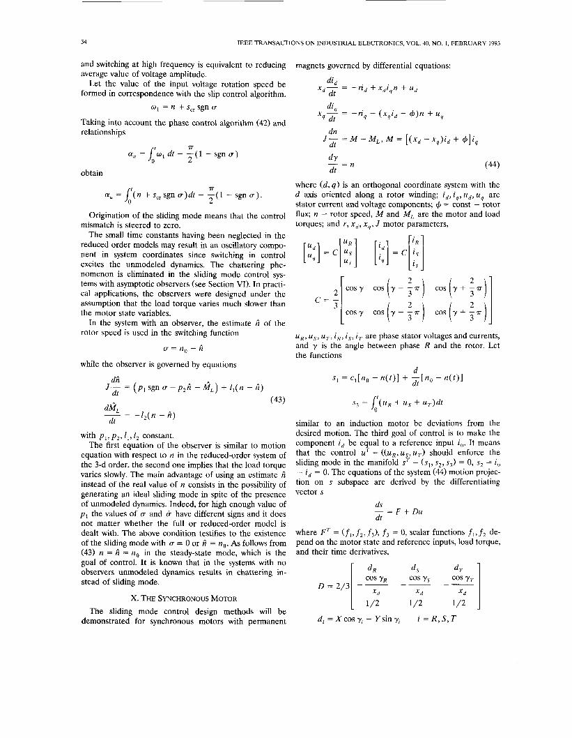
Let the value of the input voltage rotation speed be formed in correspondence with the slip control algorithm.
w1 = n + s,, sgn a
Taking into account the phase control algorithm (42) and relationships
IT C Y , = ( w , dt - -(1 - sgn a )
2
obtain
?r C Y , = l ( n + s,, sgn u ) d t - -(1 - sgn a ) .
2
Origination of the sliding mode means that the control mismatch is steered to zero.
The small time constants having been neglected in the reduced order models may result in an oscillatory compo- nent in system coordinates since switching in control excites the unmodeled dynamics. The chattering phe- nomenon is eliminated in the sliding mode control sys- tems with asymptotic observers (see Section VI). In practi- cal applications, the observers were designed under the assumption that the load torque varies much slower than the motor state variables.
In the system with an observer, the estimate A of the rotor speed is used in the switching function
u = n o - A
while the observer is governed by equations
dh J - = ( p , sgn u - p , ~ - kL) + l ,(n - A)
dt
d k L - - - -l,(n - A )
dt
(43)
with pl, p , , I,, 1, constant. The first equation of the observer is similar to motion
equation with respect to n in the reduced-order system of the 3-d order, the second one implies that the load torque varies slowly. The main advantage of using an estimate A instead of the real value of n consists in the possibility of generating an ideal sliding mode in spite of the presence of unmodeled dynamics. Indeed, for high enough value of p 1 the values of u and 6 have different signs and it does not matter whether the full or reduced-order model is dealt with. The above condition testifies to the existence of the sliding mode with a = 0 or A = no. As follows from (43) n = A = no in the steady-state mode, which is the goal of control. It is known that in the systems with no observers unmodeled dynamics results in chattering in- stead of sliding mode.
X. THE SYNCHRONOUS MOTOR The sliding mode control design methods will be
demonstrated for synchronous motors with permanent
magnets governed by differential equations:
did xd- = - ~ d f x i n f ud dt d q
- n dY _ - dt (44)
where (d, q ) is an orthogonal coordinate system with the d axis oriented along a rotor winding; i d , i,, u d , U , are stator current and voltage components; $ = const - rotor flux; n - rotor speed, M and ML are the motor and load torques; and r , xd, x,, J motor parameters,
U , , us, uT, i,, is, i, are phase stator voltages and currents, and y is the angle between phase R and the rotor. Let the functions
Sg = [(U, f Us + U,)dt
similar to an induction motor be deviations from the desired motion. The third goal of control is to make the component id be equal to a reference input io. It means that the control uT = ((U,, us, U , ) should enforce the sliding mode in the manifold sT = (sl, s,, s,) = 0, s2 = io - id = 0. The equations of the system (44) motion projec- tion on s subspace are derived by the differentiating vector s
ds dt - = F + + u
where F T = (f,, f,, f3), f3 = 0, scalar functions f,, f2 de- pend on the motor state and reference inputs, load torque, and their time derivatives,
dT 1
UTKIN: SLIDING MODE CONTROL DESIGN PRINCIPLES 35
x= - [ ( ‘ d - x q ) / J x d ] Zq
Y = -(l/J x,)[(x, - xy)i, + 4. The discontinuous control is designed within the frame-
work of the induction motor control design method dis- cussed in Section IX:
U = -U,, sign s* s* = DTs
Only the ranges of plant parameters and disturbances should be known to find necessary magnitudes of phase voltages to generate the sliding mode in the manifold s = 0 with desired dynamics.
The choice of the reference input i,, is usually dictated by requirements for a motor static mode. For instance, a motor torque is maximal if
Because in real-life conditions the stator current is always bounded, for i, =f(i,) enforcing sliding mode in the surface s2 =_O enables maximization of a motor torque. In many cases q2 P 4(x, - x , ) i , and then i,, = 0. Similarly, minimization of heat losses and maximization of motor efficiency may be provided by a proper choice of the reference input i,,.
The design method under discussion implies that angle position and speed and phase currents are measured directly while an acceleration d n / d t may be found with the help of the above asymptotic observer. From the point of practical applications it is of interest to design a ctntrol system with no current transducers. Let i,, and i, be estimates of stator currents components and satisfji the observer equations
d;,
dt x - = - r i d + x d i , n + U,,
and, corTespondingly, equations for mismatches iYd = Ld - i d , i, = i, - i, are of the form
did dt
xd- = - r id + x i n d 4
4 di = -n, - x , i , n .
dt
Calculate the time derivative of the Lyanpunov function U = 0.5(ii + E:) > 0 taking into account inequality x,, > Y
hence du/dt 5 -(2r/x,)u, which testifies to exponential convergence of U to zero and the observer state to real values of stator current components.
XI. CONCLUSION The paper has outlined the mathematical background
and sliding mode control design philosophy oriented to high-dimensional nonlinear systems operating under un- certainty conditions and has demonstrated its applicability to control of different types of electric motors. The elec- tric drives with sliding mode control have already been used in many applications: metal-cutting machine tools (feed and spindle drives), robotics (tracking position and speed control of manipulator links), transport (battery- driven cars and trams), and process control (fiber drafting process) 131, [61.
An assessment of the scientific arsenal accumulated in the sliding mode control theory is beyond the scope of the paper therefore we confine ourselves to mentioning new research areas initiated by scientific groups of many coun- tries: geometric approach to design, control of infinite- dimensional (including distributed and time-delay) plants, sliding mode in discrete-time systems, Lyapunov function based design methods, control of power electronic con- verters, aircraft, and combustion engines.
REFERENCES A. Bakakin, M. Gritsenko, and N. Kostyleva, “Control algorithms for variable structure systems,” Variable Structure Systems and Their Uve in Flight Automation Problems. Moscow: Nauka, pp. 13-25 (in Russian), 1968. V. 1. Utkin, “Variable structure systems with sliding modes,” IEEE Trans. Automat. Contr., vol. AC-22, no. 2, pp. 212-222, 1977. -, “Discontinuous control systems: State of the art in theory and applications,” Preprints of the 10th IFAC Congress, Germany, Munich, 1987, pp. 75-94. R. A. DeCarlo, S. H. Zak, and G. P. Matthews, “Variable structure control of nonlinear multivariable systems: A tutorial,” Proc. IEEE, vol. 76, no. 3, pp. 212-232, March 1988. V. 1. Utkin and N. E. Kostyleva, “Design principles for algorithms of local automation systems with variable structure,” Izmerenie, Control, Automatizatziya, no. 1, pp. 27-35, 1981, (in Russian). V. I . Utkin, A. S. Vostrikov, S. A. Bondarev et al., “Applications of sliding modes in automation of technological phnts,” Izmerenie, Control, Automatizatziya, no. 1, pp. 74-84, 1985, (in Russian). S. V. Emel’yanov, Variable Structure Automatic Control Systems. Moscow: Nauka, 1967 (in Russian). S. V. Emel’yanov, Ed., Theor)? of Variable Structure Systems. Moscow: Nauka, 1970 (in Russian). V. 1. Utkin, Sliding Modes and Their Applications in Variable Struc- ture Syytems. Moscow: Nauka, 1974 (in Russian), and Moscow: Mir-Publisher, 1978 (in English). K. K. Zhil’tsov, Approximation Methods of Variable Structure System Design. Moscow: Nauka, 1974 (in Russian). V. I. Utkin, Sliding Modes in Optimization and Control. Moscow: Nauka, 1981 (in Russian) and New York: Springer-Verlag, 1992 (in English). A. S. I. Zinober, Ed., Deterministic Control of Uncertain Systems. London: Peter Pcregrinus Ltd., 1990. A. A. Andronov, A. A. Vitt, and S. E. Khaikin, Theoiy of Oscd[a- lions. Moscow: Fizmztgiz, 1959 (in Russian). V. 1. Utkin, “Equations of slipping regime in discontinuous sys- tems. I , 11,” Aut. Remote Contr.,vol. 32, no. 12, pt. 1, pp. 1897-1907, 1971, vol. 33, no. 2, pt. I , IY71, pp. 211-219. A. G. Luk’yanov and V. 1. Utkin, “Methods of reducing equations of dynamic systems to a regular form,” Aut. Remote Contr., vol. 42, no. 4, pt. I , 1981, pp. 413-420. V. I. Utkin and K.-K.D. Young, “Methods for constructing discon-
36
[201
1211
[221
[231
IEEE TUNSACTIC
tinuity planes in multidimensional structure variable systems,” Aut. Remote Contr., vol. 39, no. 10, pt. 1, 1978, pp. 1466-1470. B. Drazenovic, “The invariance conditions in variable structure systems,” Automafica, vol. 5, no. 3, pp. 287-295, 1969. P. V. Kokotovic, R. B. O’Malley, Jr., and P. Sannuti, “Singular perturbation and order reduction in control theory,” Automafica,
A. G. Bondarev, S. A. Bondarev, et al. ., “Sliding modes in systems with asymptotic state observers,” Aut. Remofe Contr., vol. 46, no. 6,
J. J. Slotine and S. S. Sastri, “Tracking control of nonlinear systems using sliding surfaces, with applications to robot manipula- tor,” Inf. J. Contr., vol. 38, no. 2, pp. 465-492, 1983. J. J. Slotine, “Sliding controller design for nonlinear systems,” Int. J. Contr., vol. 40, no. 2, pp. 421-434, 1984. J. A. Burton and A. S. I. Zinober, “Continuous approximation of variable structure control,” Inc. J. System Sci., vol. 17, no. 6, pp.
D. B. Izosimov, B. Matic, et al., “Using sliding modes in control of electrical drives,” Dokl. ANSSSR, vol. 241, no. 4, pp. 769-772, 1978. (In Russian). Y. Dote and R. C. Hoft, “Microprocessor based sliding mode controller for dc motor control drives,” in IEEE U S Con$ Rec., Cincinnati, OH, 1980. A. Sabanovic and D. Izosimov, “Application of sliding modes to induction motor control,” IEEE Trans. Industiy Applications, vol. LA-17, no. 1, pp. 41-49, 1981. A. Sabanovic, D. Izosimov, 0. Music, and F. Bilalovic, “Sliding modes in controlled motor drives,” in Proc. IFAC Conf. on Control in Power Electronics and Electrical Drice~, Lausanne, Switzerland, 1983, pp. 133-138. F. Harashima, H. Hashimoto, and S. Kondo, “MOSFET converter- fed position servo system with sliding mode control,” IEEE Trans. Ind. Elecrron., vol. IE-32, no. 3, pp. 238-244, 1986. H. Hashimoto, H. Yamomoto, S. Yanagisava, and F. Harashima, “Brushless servomotor control using variable structure approach,” in ConJ Rec. 1986 IEEE Industry Application Society Annu. Meet., pt. 1, 1986, pp. 72-79. G. P. Matthew, R. DeCarlo, and Lefebvre, “Towards feasible variable structure control design for a synchronous machine con- nected to an infinite bus,” IEEE Trans. Automat. Contr., vol. AC-31, no. 12, 1986.
vol. 12, pp. 123-132, 1976.
pt. 1, pp. 679-684, 1985.
875-885, 1986.
INS ON INDUSTRIAL ELECTRONICS, VOL. 40, NO. 1, FEBRUARY 1993
[30] D. B. Izosimov, “Sliding-mode nonlinear state observer of an induction motor,” in Control of Multiconnected Systems, M. V. Meerov and N. A. Kuznetsov, Eds. Moscow: Nauka, pp. 133-139, 1983, (in Russian).
[31] Y. Dote, T. Manabe, and Murakami, “Microprocessor-based force control for manipulator using variable structure with sliding mode,” in Proc. IFAC Conf: on Control in Power Electronics and Electrical DriL,es, Lausanne, Switzerland, 1983, pp. 145- 149.
[32] F. Harashima, H. Hashimoto, and K. Maruyama, “Practical robust control of robot arm using variable structure control,” in Proc. 1986 IEEE Int. Conf: on Robotics and Automation, Apr. 7-10, San Francisco, pp. 532-539, 1986. H. Hashimoto et al., “Sliding mode control of induction motors based on reduced order models,” in Korean Automatic Control Con$, vol. 2, pp. 1607-1610, 1991.
[33]
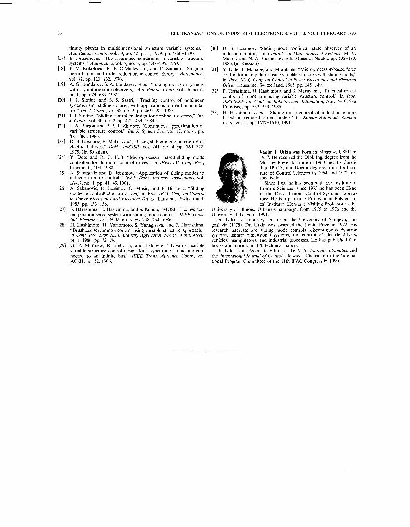
Vadim 1. Utkin was born in Moscow, USSR in 1937. He received the Dipl. Ing. degree from the Moscow Power Institute in 1960 and the Candi- date (Ph.D.) and Doctor degrees from the Insti- tute of Control Sciences in 1964 and 1971, re- spectively.
Since 1960 he has been with the Institute of Control Sciences, since 1973 he has been Head of the Diwmtinuous Control Systems Labora- tory He is d part-time Professor at Polytechni- cal Institute He was a Visiting Professor at the
University of Illinois, Urbana-Champaign, from 1975 to 1976 and the University of Tokyo in 1991.
Dr. Utkin is Honorary Doctor at the University of Sarajevo, Yu- goslavia (1978). Dr. Utkin was awarded the Lenin Prize in 1972. His research interest$ are sliding mode controls, discontinuous dynamic systems, infinite dimensional systems, and control of electric drivers, vehicles, manipulators, and industrial processes He has published four books and more than 170 technical papers.
Dr. Utkin is an Associate Editor of the IFAC JournalAutomatica and the Intemational Journal of Control He was a Chairman of the Interna- tional Program Committee of the l l th IFAC Congress in 1990.


![Sliding mode control design principles and applications …eusai/BOSIO/[7]-Utkin-TIE-1993.pdf · Sliding Mode Control Design Principles and Applications to Electric Drives ... SLIDING](https://static.documents.pub/doc/80x56/5b8e42d909d3f2a8408d4ff4/sliding-mode-control-design-principles-and-applications-eusaibosio7-utkin-tie-1993pdf.jpg)
![Robust Fuzzy-Second Order Sliding Mode based …thesai.org/...Robust_Fuzzy_Second_Order_Sliding_Mode_based...Con… · Robust Fuzzy-Second Order Sliding Mode based ... [3]. Sliding-mode](https://static.documents.pub/doc/80x56/5b7a16407f8b9a483c8b5dce/robust-fuzzy-second-order-sliding-mode-based-robust-fuzzy-second-order-sliding.jpg)


