Sliding Mode Control for a Vertical Dynamics

in the Presence of Nonlinear Friction

TOBIAS FERCH and PAOLO MERCORELLI

Institute of Product and Process Innovation

Leuphana University Lueneburg

Universitätsallee 1, 21335 Lueneburg, Germany

mercorelli@uni.leuphana.de

Abstract: - This paper deals with a control of a vertical dynamics in the presence of nonlinear friction in a

robotic mechanism. The control structure, which is taken into consideration, is the Sliding Mode Control

(SMC). Using this control technique, it is possible to show the asymptotical stability of the trajectory to be tracked. Simulation results show the effectiveness of the proposed control technique.

Key-Words: - Mechanical systems - Mechanical friction – Displacement - SMC – Applications - Simulations

1 Introduction

In the course of Industry 4.0, the use of robotic

systems in industrial manufacturing is increasingly

playing an essential role. Moreover, the use of industrial robots is based on the guaranteed

uniformity and precision that such a system offers.

In this case, the robot can do different tasks. For example, it can be used independently in series

production or supportive and it can serve the person

as a helper at work. The articulated robots used in industry are usually constructed as an open

kinematic chain. In this design, each arm part of the

robot is connected via a joint to the following arm

part. The last arm part of the chain is called the effector: this is the part of the robot that interacts

with the environment. Tasks in which the effector

enters into mechanical contact with objects within its environment are normal. Therefore, the contact

force plays an essential role in the control of such

systems. Since industrial robots are mainly operated position-controlled, the control of the contact force

and the position control are related to each other. In

order to move an object from its starting position to

the target position, individual or cooperating robots are used in industrial production, these have as

effector predominantly a variant of a gripper. The

joint gripping of an object offers the advantage of load sharing, in contrast, this also leads to the

closing of a kinematic chain between the two robots.

As a result of this connection, the two robots

mutually influence each other during their

movement, as a result of which undesired changes

in the relative robot position can occur, resulting in resultant forces in the workpiece. To avoid this

problem, this work deals with the clawless position

control of an object. In this case, an articulated robot

is considered, which regulates the vertical position of an object solely by the applied contact pressure.

In this case, the actual position of the object centre

point should follow the desired set point position in a uniform movement. The control was realized with

a Sliding Mode Control (SMC), this method offers

the necessary flexibility and robustness to enable a valid analysis, in particular in an application field,

[1], [2], [3]. The paper is organized as follows. In

Section 2 some physical basic knowledge are

considered. Section 3 considers the construction of the model using differential equations. Section 4

presents the obtained results. Discussion, conclusion

and outlook close the paper.

2 Background

For simplification, the object is pressed against a

rigid surface by the robot arm (Fig.1). One possible

type of control of an articulated robot is the path control. In this motion control, from given velocity

and acceleration, orbits are calculated with respect

to the effector in the world coordinate system. The path control enables a movement on a straight line

with the aid of linear interpolation. Here, the centre

of the effector (also called TCP = Tool Centre

WSEAS TRANSACTIONS on CIRCUITS and SYSTEMS Tobias Ferch, Paolo Mercorelli

E-ISSN: 2224-266X 102 Volume 18, 2019

Point) serves as a reference point for the movement

on the linear path. This type of motion allows

viewing robot dynamics in the horizontal plane,

starting from the centre of the effector. The contact forces, due to Coulomb friction, provide a

nonlinearity of dynamics. One of the core tasks is

the modelling of the dynamics in order to be able to simulate system behaviour close to reality..

Figure 1: Schematic representation of robotic arm and

object

The field of control engineering makes it possible to

describe the behaviour of dynamic systems based on

their signals and the transformations of these signals. Signals are time-variable quantities which

are processed and transmitted by a dynamic system.

Because of this, differential equations typically form the basis of models. These contain signals and their

time derivatives, as well as system-dependent

physical parameters. The established differential equations make it possible to determine the time

course of the output variable as a function of the

input variable. In the process, the effects of the

control parameters and the relationships of the control loop are recorded, which enables targeted

intervention in the system. In order to arrive at the

desired model via the relationships of the control loop, it is necessary to deduce the physical character

of the dynamic processes. Here, temporal processes

are described by time functions and the relationships between the processes as functional dependencies

between these time functions. The temporally

variable description variables of physical

phenomena are decisive, as they reflect the dynamic behaviour of the system under consideration. In the

following the physical basics for the derivation of

the required differential equations are presented.

2.1 Physical basics

Charles Augustine de Coulomb has shown by

experiments that as long as a horizontal force 𝐹𝑥 remains below a limit 𝐹0, then 𝐹𝐻(𝑡) = 𝐹𝑥(𝑡), where 𝐹𝐻(𝑡) represents the friction force which can

be considered in a possible movement. If the force

reaches this limit, 𝐹𝐻(𝑡)assumes its maximum value

𝐹𝐻0. Furthermore, Coulomb's experiments showed

that the normal force and the limit 𝐹𝐻0 are

proportional in a first approximation and it results as follows:

𝐹𝐻0 = 𝜇0𝐹𝑁(𝑡). (1)

The proportionality factor 𝜇0 is called the

coefficient of adhesion, which depends on the

materials of the surfaces. If the limit is exceeded, the body moves on a rough surface, while the

sliding friction force 𝐹𝑅 occurs as an impressed

force. This is opposite to the direction of movement

and is therefore also a resisting force. Since the body moves in this scenario, the basic equation of

kinetics of the mechanism results as follows:

𝑚�̈�(𝑡) = 𝐹𝑥(𝑡) − 𝐹𝑅(𝑡). (2)

Coulomb's experiments have shown that frictional

force 𝐹𝑅(𝑡) is also proportional to normal force

𝐹𝑁(𝑡) and simultaneously independent of velocity.

This results in the following basic physical law:

𝐹𝑅(𝑡) = 𝜇𝐹𝑁(𝑡). (3)

Here, the proportionality factor 𝜇 is called the friction coefficient. The two coefficients are always

less than one, hence 𝐹𝐻(𝑡) and 𝐹𝑅(𝑡) are always

fractions of the normal force 𝐹𝑁(𝑡). The dimension

of the factors is a material constant and is determined experimentally between two surfaces.

The foundations of tribology listed here revealed the

following findings applied to the vertical system. Since this is a dynamic scheme, these findings were

determined in a time-dependent manner. The weight

force 𝐹𝐺(𝑡), which previously pressed the body to

the plane, now acts as a driving force for the movement in the y-direction. The body is brought

into its equilibrium situation by the contact force

𝐹𝑅𝑥(𝑡), acting through the robot. The free-body

image of this system provides information about the

position of the normal force and the static friction

force:

WSEAS TRANSACTIONS on CIRCUITS and SYSTEMS Tobias Ferch, Paolo Mercorelli

E-ISSN: 2224-266X 103 Volume 18, 2019

← : 𝐹𝑁(𝑡) = 𝐹𝑅𝑥(𝑡) , ↓ : 𝐹𝐻(𝑡) = 𝐹𝐺(𝑡). (4)

According to Coulomb's laws, the limit is

approximately for the static friction force 𝐹𝐻(𝑡):

𝐹𝐻0(𝑡) = 𝜇0𝐹𝑁(𝑡) = 𝜇0𝐹𝑅𝑥(𝑡). (5)

The static friction force is thus directly dependent

on the acting contact force 𝐹𝑅𝑥(𝑡) of the robot. In

the equilibrium position of the system the following relations hold:

𝐹𝐻(𝑡) = 𝜇𝐻𝐹𝑅𝑥(𝑡), (8)

𝐹𝐻(𝑡) > 𝐹𝐺(𝑡) . (9)

Accordingly, if the robot exerts a contact force

𝐹𝑅𝑥(𝑡) which, in conjunction with the static friction

coefficient 𝜇𝐻, is greater than the weight of the

body, it is prevented from moving. If this is not the case, the body moves in the positive y-direction

defined here. From the basic equation of the kinetics

follows:

𝑚�̈�(𝑡) = 𝐹𝐺(𝑡) − 𝐹𝐻(𝑡) = 𝑚𝑔 − 𝑘𝐻𝐹𝑅𝑥(𝑡), with

static friction coefficient 𝑘𝐻 (10)

𝑚�̈�(𝑡) = 𝐹𝐺(𝑡) − 𝐹𝑅(𝑡) = 𝑚𝑔 − 𝑘𝑅𝐹𝑅𝑥(𝑡) with

coefficient of friction 𝑘𝑅. (11)

2.2 The viscoelasticity

The horizontally acting force of the robot 𝐹𝑅𝑥(𝑡) causes deformation of the body, any deformation or

return of a body is time-dependent. If the load is

released, a time-dependent complete recovery of the material is called viscoelasticity. This behaviour can

be simplified with the help of a Kelvin-Voigt

element (Fig. 2). [4]

Figure 2: Parallel connection spring and damper element

To determine the behaviour of viscoelastic

materials, characteristic material functions are

experimentally developed. Viscoelastic fabrics have both elastic and viscous properties.

The viscoelastic factors are cumulated in this

constant in the constant 𝑘𝑐. From the factor of

viscoelasticity and the movement of the centre of mass in the x-direction, this relationship results for

the viscoelastic resistance 𝐹𝑐(𝑡):

𝐹𝑐(𝑡) = 𝑘𝑐𝑥𝑚(𝑡). (18)

2.3 The flow resistance The body of the object is flowed around by the fluid air, the body prevents the fluid particles from

flowing straight along the streamlines. As a result,

the fluid is deflected and flows past the body. Now, as the body moves through the fluid, it creates a

resistive force that counteracts the movement of the

body. In contrast to the Coulomb friction, the

resistance increases with increasing speed. Other influencing factors are the shape of the body and the

fluid properties of the fluid. At low speeds, there is

approximately a proportionality between speed and drag. At higher speeds, the force increases in

proportion to the square of the speed. Assuming

gravity to be constant and accelerating the object down from rest, the equation for flow resistance is

given:

𝐹𝐿(𝑡) = 𝑏|𝑣(𝑡)|𝑛 (19)

with 𝑏 und 𝑛 being constants.

This general formula of flow resistance begins to become inaccurate even at speeds of a few meters

per second. With the help of the Bernoulli equation,

an equation can be derived which has a much higher

accuracy. Assuming that the body around which it flows lowers the velocity of the fluid directly behind

the body to zero, the pressure difference between

the faces perpendicular to the flow direction results: Figures and Tables should be numbered as follows:

∆𝑝 =1

2𝜌𝑣(𝑡)2. (20)

Since 𝑝 = 𝐹/𝐴, the drag force can be calculated

based on the dynamic pressure. From this

WSEAS TRANSACTIONS on CIRCUITS and SYSTEMS Tobias Ferch, Paolo Mercorelli

E-ISSN: 2224-266X 104 Volume 18, 2019

assumption, the general formula for the Newtonian

resistance force follows:

𝐹𝐿(𝑡) =1

2𝑐𝐴𝜌𝑣(𝑡)2. (21)

The constant c is the coefficient of resistance, this refers to the entire shape of the body and is

determined experimentally. Since the shape of the

body and the material properties can be neglected in the course of this research work, the following

forms can be derived from the laws listed here:

𝐹𝐿(𝑡) = 𝑘𝐿𝑣(𝑡). (22)

The factor 𝑘𝐿 is a constant which includes all

system-specific factors and serves as a substitute for them. Thus, the flow resistance is only in proportion

to this factor and the respective speed. From this

form results for the dynamics in the x- and y-direction:

𝐹𝐿𝑦(𝑡) = 𝑘𝐿𝑦�̇�(𝑡) and

𝐹𝐿𝑥(𝑡) = 𝑘𝐿𝑥�̇�(𝑡). (23)

3 Modelling

The physical phenomena and laws listed in the

previous section allow to set up the necessary

differential equations, which serve as a basis for the subsequent modelling. When setting up a

differential equation, basically four steps can be

used. In the first step, the system is broken down into its individual components. Subsequently, the

physical laws are formulated, which describe the

behaviour of the components. This step was already

done in the previous section. In the third step, the coupling relationships between the components are

established, and in the final, fourth step, the

determined equations are then combined to form a differential equation. Since the target is the position

control of the object in the vertical plane, three

differential equations are needed in total.

3.1 DGL Ⅰ horizontal dynamics of the robot

Figure 3: Free cut robot arm

The cut-out in Fig. 3 provides the position of the

forces on the robot arm:

← : 0 = 𝐹𝑅𝑥(𝑡) − 𝑘𝑐𝑥𝑅(𝑡) − 𝑘𝐿𝑥�̇�𝑅(𝑡), (24)

with 𝑥𝑅(𝑡) as the movement of the robot in the

positive x-direction and �̇�𝑅(𝑡) as the associated

movement speed. The origin of the coordinate system lies at the centre of the tool tip, as shown in

the figure above. The resistance of the air and the

resistance of the viscoelasticity counteract pressure of the robot. In conjunction with the basic equation

of kinetics, the following differential equation

results:

𝑚𝑅�̈�𝑅(𝑡) = ∑ 𝐹𝑥 (𝑡), (25) 𝑚𝑅�̈�𝑅(𝑡) = 𝐹𝑅𝑥(𝑡) − 𝑘𝑐𝑥𝑅(𝑡) − 𝑘𝐿𝑥�̇�𝑅(𝑡). (26)

3.2 DGL Ⅱ horizontal dynamics of the object

Figure 4: Free cut object horizontal

The free-body image in Fig. 4 shows the position of the forces between the robot arm and the object:

WSEAS TRANSACTIONS on CIRCUITS and SYSTEMS Tobias Ferch, Paolo Mercorelli

E-ISSN: 2224-266X 105 Volume 18, 2019

← : 0 = 𝑘𝑐𝑥𝑅(𝑡) − 𝑘𝑐𝑥𝑚(𝑡) + 𝑘𝐿𝑥�̇�𝑅(𝑡)− 𝑘𝐿𝑥�̇�𝑚(𝑡)

0 = 𝑘𝑐(𝑥𝑅(𝑡) − 𝑥𝑚(𝑡)) + 𝑘𝐿𝑥(�̇�𝑅(𝑡)

−�̇�𝑚(𝑡)),

(27)

with 𝑥𝑚(𝑡) as movement of the mass in positive x-

direction and �̇�𝑚(𝑡) as associated movement speed. These assumptions are to be considered in the

context of the DGL. The movement of the robot arm

causes a deformation of the object and thus moves the centre of gravity of the body. Under these

conditions the following dynamic behaviour results:

𝑚�̈�𝑚(𝑡) = ∑ 𝐹𝑥 (𝑡) (28) (1)

𝑚�̈�𝑚(𝑡) = 𝑘𝑐(𝑥𝑅(𝑡) − 𝑥𝑚(𝑡))

+𝑘𝐿𝑥(�̇�𝑅(𝑡) − �̇�𝑚(𝑡)). (29)

(Ⅱ)

As a result, the horizontal movement of the centre of mass counteracts the flow resistance of the air and

its own viscoelastic properties. These forces are

directly related to the movement of the robot arm.

3.3 DGL Ⅲ vertical dynamics of the object

Figure 5: Free-cutting object vertical

The free-body image in Fig. 5 provides the forces

acting vertically on the body:

↓ : 0 = 𝑚𝑔−𝐹𝐻(𝑡) − 𝑘𝐿𝑦�̇�𝑚(𝑡) at rest (30) (2)

↓ : 0 = 𝑚𝑔−𝐹𝑅(𝑡) − 𝑘𝐿𝑦 �̇�𝑚(𝑡) in motion. (31) (3)

If the weight force 𝐹𝐺(𝑡) is below the limit value of

the adhesive condition, the body remains in its

equilibrium position. If the limit of static friction is exceeded, the body starts to move. This movement

counteracts the resistance of Coulomb friction and

slows down the body. Furthermore, the flow

resistance of the air counteracts the movement. Information about the dynamic behaviour provides

again the basic equation of the kinetics:

𝑚�̈�𝑚 (𝑡) = ∑ 𝐹𝑦 (𝑡) (32)

𝑚�̈�𝑚 (𝑡) = 𝑚𝑔−𝐹𝐻(𝑡) − 𝑘𝐿𝑦�̇�𝑚(𝑡) (33)

𝑚�̈�𝑚 (𝑡) = 𝑚𝑔−𝐹𝑅(𝑡) − 𝑘𝐿𝑦�̇�𝑚(𝑡). (34)

4 The Sliding Mode Control

SMC is one of the most important control strategies

in the field of nonlinear control, [5], [6], [7], [8] and

[9].

The switching function of the dynamics results from

the following general basic equation:

𝑠(𝑡) = (𝑑

𝑑𝑡+ 𝑘𝑠)

𝑛−1

∆𝑥(𝑡) with

∆𝑥(𝑡) = 𝑥(𝑡) − 𝑥𝑑(𝑡). (35)

The goal is to control the position of the body in a

vertical plane. For these dynamics a differential

equation of the second order exists, from which it follows with n = 2:

𝑠(𝑡) = (𝑑

𝑑𝑡+ 𝑘𝑠)∆𝑦(𝑡). (36)

WSEAS TRANSACTIONS on CIRCUITS and SYSTEMS Tobias Ferch, Paolo Mercorelli

E-ISSN: 2224-266X 106 Volume 18, 2019

𝑠(𝑡) = �̇�𝑚(𝑡) − �̇�𝑚𝑑(𝑡)

+ 𝑘𝑠(𝑦𝑚(𝑡) − 𝑦𝑚𝑑(𝑡)).

(36)

The following Lyapunov function is suitable for this

switching function, with the condition

𝑉(0) = 0. (37)

Considering

𝑉(𝑠(𝑡)) =1

2𝑠2(𝑡). (38)

This function satisfies the condition 𝑉(𝑡) > 0 of

Lyapunov, the differentiation of this function leads

to:

�̇�(𝑠(𝑡)) = 𝑠(𝑡)�̇�(𝑡). (39)

This corresponds to the desired shape. The insertion

of the sliding surface leads to:

�̇�(𝑡) = 𝑠(𝑡)[�̈�𝑚 (𝑡) − �̈�𝑚𝑑 (𝑡) + 𝑘𝑠(�̇�𝑚(𝑡)

− �̇�𝑚𝑑(𝑡))].

(40)

Subsequent insertion of the equation (33) for

�̈�𝑚 (𝑡):

�̇�(𝑡) = 𝑠(𝑡) [𝑔 −𝐹𝐻(𝑡) − 𝑘𝐿𝑦�̇�𝑚(𝑡)

𝑚

− �̈�𝑚𝑑 (𝑡) + 𝑘𝑠(�̇�𝑚(𝑡)

− �̇�𝑚𝑑(𝑡))]

(41)

And the substitution of 𝐹𝐻(𝑡) leads to:

0 = 𝑔 −𝐹𝐻(𝑡)−𝑘𝐿𝑦�̇�𝑚(𝑡)

𝑚− �̈�𝑚𝑑 (𝑡) + 𝑘𝑠(�̇�𝑚(𝑡)-

�̇�𝑚𝑑(𝑡)) (42)

𝐹𝐻(𝑡) = −𝑘𝐿𝑦�̇�𝑚(𝑡) + 𝑚[−�̈�𝑚𝑑 (𝑡) +

𝑘𝑠(�̇�𝑚(𝑡) − �̇�𝑚𝑑(𝑡)) + 𝑔].

(43)

Taking into account the following relation:

𝐹𝐻(𝑡) = −𝑘𝐿𝑦�̇�𝑚(𝑡) + 𝑚[−�̈�𝑚𝑑 (𝑡) +

𝑘𝑠(�̇�𝑚(𝑡) − �̇�𝑚𝑑(𝑡)) + 𝑔] + 𝑚𝜆𝑠(𝑡) +

𝑚𝐵𝑠𝑔𝑛(𝑠(𝑡)). (44)

Subsequent insertion of the substitution term in

�̇�(𝑡):

�̇�(𝑡) = 𝑠(𝑡)[−𝜆𝑠(𝑡) − 𝐵𝑠𝑖𝑔𝑛(𝑠(𝑡))]. (45)

With the condition 𝜆, 𝐵 > 0 it follows:

WSEAS TRANSACTIONS on CIRCUITS and SYSTEMS Tobias Ferch, Paolo Mercorelli

E-ISSN: 2224-266X 107 Volume 18, 2019

�̇�(𝑡) = −𝜆𝑠(𝑡)2 − 𝐵|𝑠(𝑡)| < 0. (46)

The stability condition of Lyapunov is thus fulfilled and also the asymptotic stability of the rest position.

The relationship between the contact force 𝐹𝑅𝑥(𝑡) and the static friction force 𝐹𝑅𝑥(𝑡) is given by:

𝐹𝐻(𝑡) = (𝐹𝑅𝑥(𝑡) − 𝑘𝑐(𝑥𝑚(𝑡) − 𝑥𝑅(𝑡))𝑘𝐻 . (47)

The required contact force to produce the stiction

state is thus defined by:

𝐹𝑅𝑥(𝑡) =𝐹𝐻(𝑡)

𝑘𝐻+ 𝑘𝑐(𝑥𝑚(𝑡) − 𝑥𝑅(𝑡)).

(48)

Inserting the switching function leads to:

𝐹𝑅𝑥(𝑡)

= 𝑘𝑐(𝑥𝑚(𝑡) − 𝑥𝑅(𝑡))

+−𝑘𝐿𝑦�̇�𝑚(𝑡) + 𝑚[−�̈�𝑚𝑑 (𝑡) + 𝑘𝑠(�̇�𝑚(𝑡) − �̇�𝑚𝑑(𝑡))]

𝑘𝐻

+m[+𝑔+𝜆𝑠(𝑡)+𝐵𝑠𝑔𝑛(𝑠(𝑡))]

𝑘𝐻]. (49)

Thus, a SMC was derived taking into account the stability theory of Lyapunov and the reachability

condition of the switching hyperplane. With the help

of this it is now possible to control the actual position of the object solely on the basis of the

desired position.

5 Simulations

It is used to vary parameters in the course of the

investigation in order to analyse the control and in order to show how the disturbance can influence the

behaviour of the controlled system.

Figure 6: Target (blue line) and actual position (red line)

• All graphs of the actual position are marked with a red colour

• All graphs of the nominal position are marked with

the blue colour.

The function graphs in Fig. 6 show the behaviour

between the set point and the actual position. The

simulation time was set at ten seconds and the desired movement of the body was defined to 10

mm. The desired position is asymptotic in the

approach to the target position. However, it is also clear that the entire sequence of movements is not a

uniform movement, in addition to the target position

is not fully achieved. With the parameters λ and B,

the SMC has tuning parameters, which offer the possibility of optimizing the SMC and thus

smoothing the present motion sequence. A

significant change in the system behaviour in the range λ, B <1, could not be determined.

Figure 7: Simulation for λ = 100

WSEAS TRANSACTIONS on CIRCUITS and SYSTEMS Tobias Ferch, Paolo Mercorelli

E-ISSN: 2224-266X 108 Volume 18, 2019

It was therefore necessary to investigate how the

dynamics change when the parameters in the range

λ, B> 1 are increased in detail and in connection.

First the behaviour of the function graph at a constant value of B = 1 and the change of λ is

investigated. Setting λ = 100 produces the result

graphed in Fig. 7. The achievement of the desired position is thereby not possible. However, some

increase in the switching frequency during the

sliding phase of the switching function which is noticeable. Of interest is now the behaviour of the

function with further increase of the factor. The

function graph in Fig. 8 corresponds to the

behaviour at λ = 1000. The actual position follows here approximately the desired position on the entire

route. The movement provides a much more stable

pattern along the entire route. When enlarging the graphs, however, it became clear that even here the

target position is not completely reached. There is a

small difference between the actual value and the set point value every time t.

∆𝑦(𝑡) = 𝑦𝑚(𝑡) − 𝑦𝑚𝑑(𝑡) > 0. (50)

By simply tuning the parameter λ, the sliding

surface cannot be met.

Figure 8: λ = 1000

It was therefore necessary to investigate whether and to what degree the parameter B can improve the

system behaviour in terms of control. As in the

previous analysis, the value of a parameter is kept constant, here λ = 1. The function graph in Fig. 9

shows the system behaviour with a parameterization

of B = 100.

Figure 9: B = 100

In contrast to the λ parameter, the B parameter does

not seem to exert a significant influence on the switching frequency of the graph. However, it is

clear that the actual position reaches the target

position asymptotically. After reaching the desired

position ∆𝑦(𝑡) = 𝑦𝑚(𝑡) − 𝑦𝑚𝑑(𝑡) = 0, the

dynamics is maintained at the switching hyperplane.

Figure 10: B = 1000

Further increasing the parameter B = 1000 gave the

result of Fig. 10. The feature now provides a significant improvement in stability during the

sliding phase. It follows that during this phase the

parameter has an influence on the rate of change of the switching function.

WSEAS TRANSACTIONS on CIRCUITS and SYSTEMS Tobias Ferch, Paolo Mercorelli

E-ISSN: 2224-266X 109 Volume 18, 2019

Figure 11: λ = 500, B = 100

It is thus proven that the connection of the two

parameters can unmistakably contribute to

achieving the desired performance. The result of the connection and tuning of the two parameters is

shown in Fig. 11. This function graph now offers

asymptotic stability during the sliding phase in the

direction of the desired position. In addition, the rate of change is designed so that the actual position

follows the desired position during the sliding phase

in an approximately uniform movement.

𝑠(𝑡)�̇�(𝑡) = −𝐵|𝑠(𝑡)| − 𝜆𝑠(𝑡)2 < 0. (51)

The values λ = 500 and B = 100 were determined

experimentally and a further optimization of the parameterization is not excluded.

5.1 Disturbance behaviour

The robustness of the SMR, in contrast to limited external disturbances, now had to be proven as well.

One potential source of interference could be

bumped on the surface of the object. The simulation

of this case was realized with the help of the Sine Wave function block. The sine wave block

generates a sinusoidal output signal, whereby the

simulation time serves as a time base. With a randomly chosen value for the amplitude, the noise

signal shown in Fig. 12.

Figure 12: Sine wave interference signal

The interference signal 𝑧(𝑡) thus generated has the

following effects on the vertical dynamics of the

object:

�̈�𝑅(𝑡) = 𝑚𝑔−𝐹𝑅(𝑡)−𝑘𝐿𝑦�̇�𝑚(𝑡)+𝑧(𝑡)

𝑚 and

�̈�𝑚(𝑡) = 𝑚𝑔−𝐹𝐻(𝑡)−𝑘𝐿𝑦�̇�𝑚(𝑡)+𝑧(𝑡)

𝑚.

(52)

Due to the prior adjustment of the sliding mode

control, there was no change in the function shown

in Fig. 11. Setting the parameters λ, B = 1 confirms the influence of the disturbance variable on the

dynamics (Fig. 13).

Figure 13: Interference Signal, λ = 1, B = 1

Of interest are the limits of λ and B, where the

control has instability. A constant parameter B =

100 and the simultaneous reduction of λ resulted in no decrease in performance up to a value of λ=389,

from which value of an instability resulted, Fig. 14.

WSEAS TRANSACTIONS on CIRCUITS and SYSTEMS Tobias Ferch, Paolo Mercorelli

E-ISSN: 2224-266X 110 Volume 18, 2019

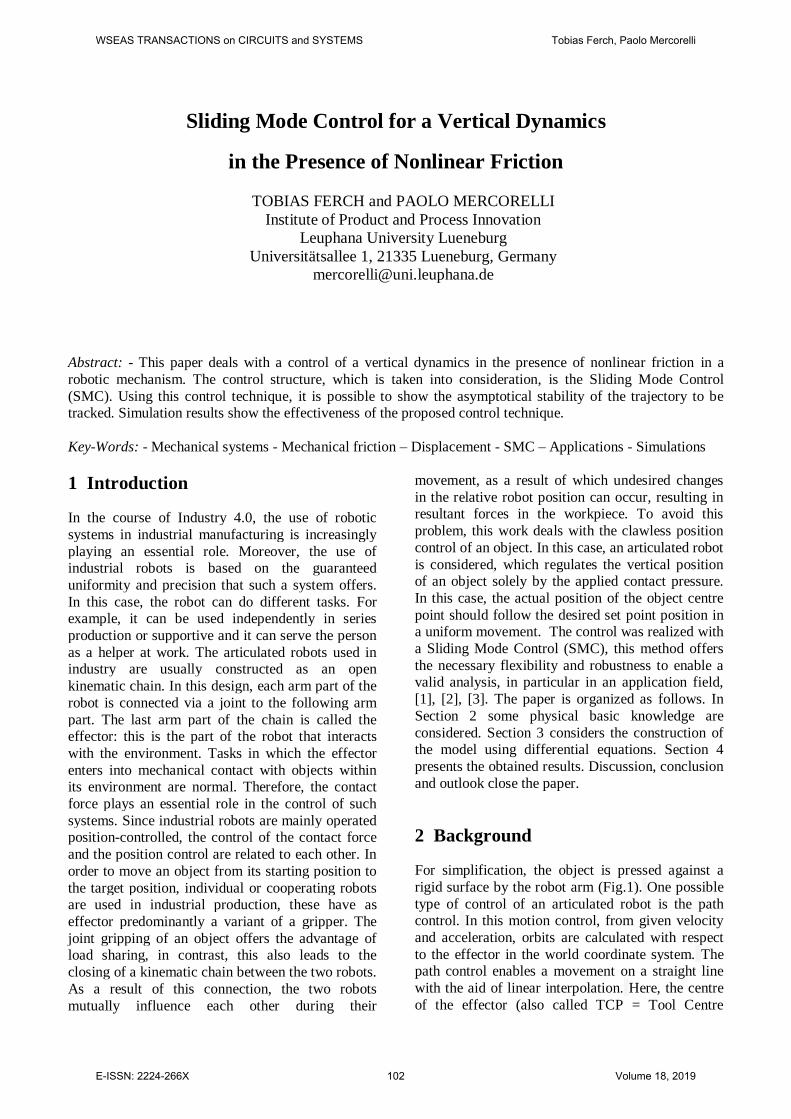
Figure 14: Interference Signal, λ = 389, B = 100

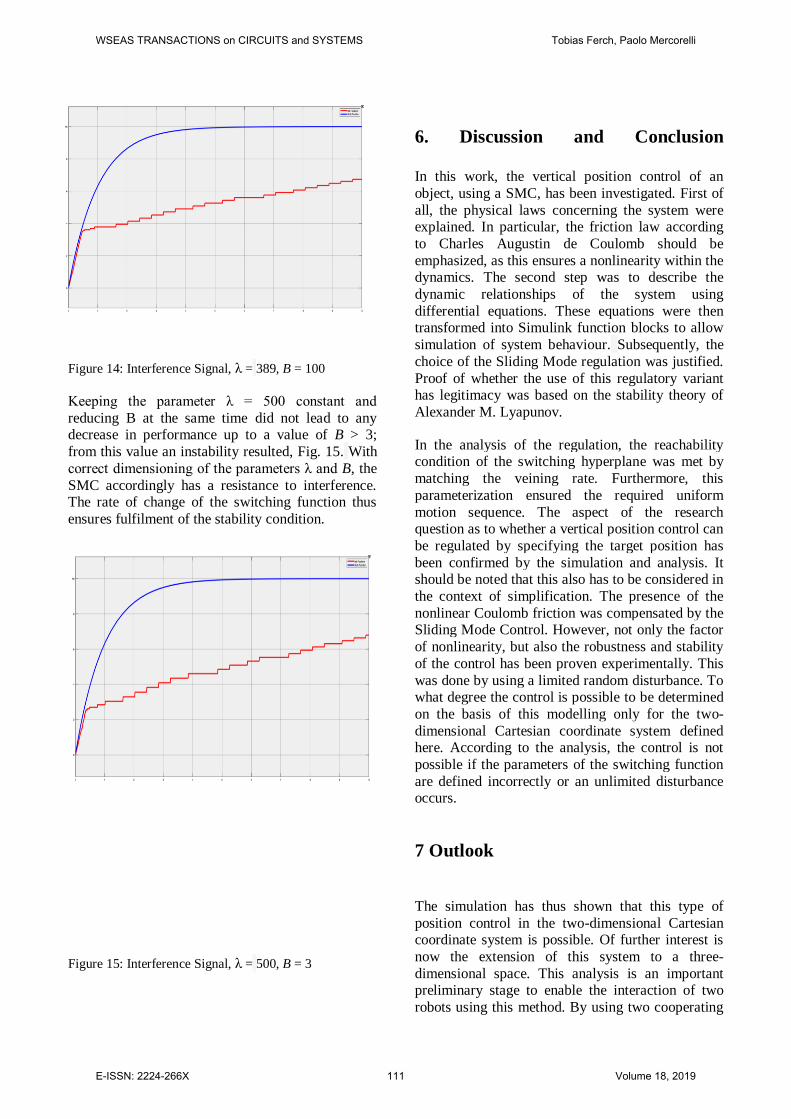
Keeping the parameter λ = 500 constant and

reducing B at the same time did not lead to any decrease in performance up to a value of B > 3;

from this value an instability resulted, Fig. 15. With

correct dimensioning of the parameters λ and B, the

SMC accordingly has a resistance to interference. The rate of change of the switching function thus

ensures fulfilment of the stability condition.

Figure 15: Interference Signal, λ = 500, B = 3

6. Discussion and Conclusion In this work, the vertical position control of an

object, using a SMC, has been investigated. First of

all, the physical laws concerning the system were explained. In particular, the friction law according

to Charles Augustin de Coulomb should be

emphasized, as this ensures a nonlinearity within the dynamics. The second step was to describe the

dynamic relationships of the system using

differential equations. These equations were then transformed into Simulink function blocks to allow

simulation of system behaviour. Subsequently, the

choice of the Sliding Mode regulation was justified.

Proof of whether the use of this regulatory variant has legitimacy was based on the stability theory of

Alexander M. Lyapunov.

In the analysis of the regulation, the reachability condition of the switching hyperplane was met by

matching the veining rate. Furthermore, this

parameterization ensured the required uniform

motion sequence. The aspect of the research question as to whether a vertical position control can

be regulated by specifying the target position has

been confirmed by the simulation and analysis. It should be noted that this also has to be considered in

the context of simplification. The presence of the

nonlinear Coulomb friction was compensated by the Sliding Mode Control. However, not only the factor

of nonlinearity, but also the robustness and stability

of the control has been proven experimentally. This

was done by using a limited random disturbance. To what degree the control is possible to be determined

on the basis of this modelling only for the two-

dimensional Cartesian coordinate system defined here. According to the analysis, the control is not

possible if the parameters of the switching function

are defined incorrectly or an unlimited disturbance occurs.

7 Outlook

The simulation has thus shown that this type of

position control in the two-dimensional Cartesian coordinate system is possible. Of further interest is

now the extension of this system to a three-

dimensional space. This analysis is an important preliminary stage to enable the interaction of two

robots using this method. By using two cooperating

WSEAS TRANSACTIONS on CIRCUITS and SYSTEMS Tobias Ferch, Paolo Mercorelli

E-ISSN: 2224-266X 111 Volume 18, 2019

robots, objects could be transported to any position

within their environment by combining both contact

forces. Since the shape, material type and start

position of the object are known in industrial production, it would be possible to define the object

centre as the origin of a coordinate system. This

would result in the robots being able to orient their centre of effect around the newly created origin of

coordinates. When moving in three-dimensional

space, rotational movements of the robots play an essential role. But not only the rotation of the robot

axes has to be considered, but also the rotation

movement of the object has to be included in the

control. Since the findings of this work were derived purely from a simulation, it goes without saying that

the practical implementation of these findings is of

great interest. This outlook shows that there is a broad spectrum for further theoretical and

experimental research based on this approach.

References: [1] Mercorelli Paolo A robust cascade sliding mode control for a hybrid piezo-hydraulic actuator in camless internal combustion engines, In IFAC

Proc. Volumes 2, pp. 790-795. [2] Zwerger Tanja, Mercorelli Paolo Combining an Internal SMC with an External MTPA Control Loop for an Interior PMSM. In Proc. of the 2018 23rd Int. Conf. on Methods and Models in Automation

and Robotics, MMAR 2018, 2018, pp. 674-679 [3] Mercorelli Paolo An antisaturating adaptive preaction and a slide surface to achieve soft landing control for electromagnetic actuators. In IEEE/ASME

Trans. on Mechatronics, vol.17, n.1, pp.76-85, 2012. [4] Rust, Wilhelm, Non-linear finite element analysis in structural mechanics, Springer, 2015

[5] Garofalo, Franco, Glielmo, Luigi, Robust Control via Variable Structure and Lyapunov Techniques, Springer, 1996

[6] Shtessel, Yuri u. a., Introduction: Intuitive Theory of Sliding Mode Control, Springer, 2014.

[7] Shtessel, Yuri, Sliding Mode Control and Observation,2014.

[8] Slotine, Jean-Jacques E./Li, Weiping, Applied nonlinear control, Prentice Hall, 1991

[9] Zinober, Alan S. I., Variable Structure and Lyapunov Control, Springer, 1994

WSEAS TRANSACTIONS on CIRCUITS and SYSTEMS Tobias Ferch, Paolo Mercorelli

E-ISSN: 2224-266X 112 Volume 18, 2019