INDUSTRY STUDIES ASSOCATION WORKING PAPER SERIES Decreasing Airline Delay Propagation by Re-Allocating Scheduled Slack By Amy Cohn Global Airline Industry Program Massachusetts Institute of Technology Cambridge, MA 02139 and University of Michigan, Ann Arbor Ann Arbor, MI 48109 [email protected]and Shervin AhmadBeygi University of Michigan, Ann Arbor Ann Arbor, MI 48109 [email protected]and Marcial Lapp University of Michigan, Ann Arbor Ann Arbor, MI 48109 [email protected]2008 Industry Studies Association Working Papers WP-2008-14 http://isapapers.pitt.edu/
Transcript
INDUSTRY STUDIES ASSOCATION WORKING PAPER SERIES
Decreasing Airline Delay Propagation by Re-Allocating Scheduled Slack
By
Amy Cohn Global Airline Industry Program
Massachusetts Institute of Technology Cambridge, MA 02139
University of Michigan, Ann Arbor Ann Arbor, MI 48109 [email protected]
and
Marcial Lapp
University of Michigan, Ann Arbor Ann Arbor, MI 48109 [email protected]
2008 Industry Studies Association
Working Papers
WP-2008-14 http://isapapers.pitt.edu/
Decreasing Airline Delay Propagation By Re-Allocating Scheduled
Slack
Shervin AhmadBeygi, Amy Cohn and Marcial LappUniversity of Michigan
April 4, 2008
Abstract
Passenger airline delays have received increasing attention over the past several years as airspacecongestion, severe weather, mechanical problems, and other sources cause substantial disruptions to aplanned flight schedule. Adding to this challenge is the fact that each flight delay can propagate to disruptsubsequent downstream flights that await the delayed flights’ aircraft and crew. This potential for delaysto propagate is exacerbated by a fundamental conflict: slack in the planned schedule is often viewedas undesirable, as it implies missed opportunities to utilize costly perishable resources, whereas slack iscritical in operations as a means for absorbing disruption. In this paper, we show how delay propagationcan be reduced by redistributing existing slack in the planning process, making minor modifications to theflight schedule while leaving the original fleeting and crew scheduling decisions unchanged. We presentcomputational results based on data from a major U.S. carrier, showing that significant improvementsin operational performance can be achieved without increasing planned costs.
1 Introduction
Airline plans are made up of several costly and constrained resources such as aircraft and crews. Theseresources link flights across the network, with each resource flowing from one flight to another. Adding tothis complexity is the fact that although each flight needs each type of resource, individual resources do notnecessarily stay linked throughout the network. For example, an aircraft and crew might be assigned to acommon flight at a particular point in the schedule, but assigned to separate flights at a later point.
One ramification of this linkage is the potential for delays to propagate. If one flight is delayed (forexample, because of a mechanical problem with the aircraft assigned to that flight), then a subsequent flightmight also be delayed because it is awaiting that inbound aircraft. The fact that resources can “split”compounds this. In Figure 1 (explained in detail in [3]) we see how a single flight delay can spread to delayseveral other flights as well.
Airline delays have increased substantially in the past 5 years (see Figure 2). The cost impact of thesedelays is substantial, including excess fuel costs (from idling aircraft), overtime pay for crew members, costsassociated with re-accommodating misconnecting passengers, as well as the lost productivity of delayedpassengers.Furthermore, the Air Transport Association has estimated that there were a total of 116.5 milliondelay minutes in 2006, resulting in a $7.7 billion increase in direct operating costs to the U.S. airline industry(see Table 1).
There are many sources for flight delays, such as mechanical problems, weather delays, ground-holdprograms, and air traffic congestion. But the secondary delays that propagate from such root delays are alsoquite substantial. For example, in November 2007, more than one-third of the delays at major U.S. airportswere the result of a late-arriving aircraft (Figure 3). Furthermore, there is a natural conflict stemming fromthe fact that slack is typically viewed as negative from the planning perspective (i.e. a waste of resources), butas positive from the operational perspective (i.e. an opportunity to absorb disruption rather than allowing
1
it to propagate). The focus of our research is therefore on determining how to incorporate the operationalissues associated with delay propagation into the airline planning process.
Table 1: Direct costs of delays in the U.S. airline industry. Costs based on data reported by U.S. passengerand cargo airlines with annual revenues of at least $100 million. Source: Air Transport Association
A key challenge in this research is the difficulty in trading off between planned costs (the cost of an airlineplan under the assumption that all flights occur as scheduled and without disruption) and operational costs(the realized cost associated with the modified plan that is implemented in response to disruptions). Giventwo different plans with varying planned costs, it is difficult to determine which of the two plans will performbetter operationally. Furthermore, it is also difficult to determine whether improvements in operationalperformance outweigh increases in planned costs, given that the plan will be operated several times (often,daily) over the planning horizon, and that potential disruptions may or may not occur during any given day.
2
0%
10%
20%
30%
40%
50%
60%
70%
80%
90%
2002 2003 2004 2005 2006 2007
year
perc
ent o
f th
e fli
ghts
Ontime (%)Delayed (%)Cancelled (%)
Figure 2: The increasing trend in delayed flights. Source: Bureau of Transportation Statistics.
Air Carrier Delay, 25.5%
Weather Delay, 3.1%
National Aviation System Delay,
37.6%
Security Delay, 0.1%
Aircraft Arriving Late, 33.6%
Figure 3: Delay causes among all major US airports in November 2007. Source: Bureau of TransportationStatistics.
3
Thus, even determining metrics for “robustness”, and then quantifying the value of these metrics (i.e. howmuch planned cost a carrier should be willing to incur to improve these metrics), are challenging researchtopics themselves that have yet to be adequately solved. The fact that the planning and operations processesare functionally separate within most carriers, with each group’s incentives aligned with different objectives,only serves to exacerbate the problem.
We therefore propose, as an interim step, to develop an approach that does not increase planned costs,but can nonetheless improve operational performance. Specifically, we propose to modify flight departuretimes so as to re-allocate the existing slack in the network. By re-timing flights, slack can be re-distributedto those flight connections that are most sensitive to disruption and thus delay propagation. We limit thetime windows in which flights can be re-timed, so as to maintain existing revenue projections. Furthermore,we restrict flight re-timings such that crew pairings remain feasible and do not change in cost. Finally,we require that the same aircraft rotations be maintained. Our computational results, based on data froma major U.S. carrier, demonstrate that this approach leads to significant improvements in expected delaypropagation without any associated increase in planned cost.
The primary contribution of our research is in developing models that can diminish delay propagationin operations, without any increase in planned costs. Our proposed models can take into account delaypropagations caused by aircraft, crew members, connecting passengers, as well as other shared resources.By demonstrating that the integrality of these models can be relaxed (i.e. that the models can be solved aslinear, rather than integer, programs), we are able to consider all down-stream impacts without sacrificingtractability. The paper is outlined as follows: In Section 2 we review the related literature. We present modelsfor re-allocating slack in Section 3, as well as a simulation model to help validate the results. Computationalexperiments are presented and analyzed in Section 4. Finally, Section 5 offers conclusions and suggestedareas for future research.
2 Literature Survey
In this section, we first briefly introduce the different steps in the airline planning process. Then we focuson different approaches to address airline delays and present related literature.
2.1 Airline Planning Problems
The airline planning process is classically decomposed into four sub-problems: schedule generation, fleetassignment, maintenance routing, and crew scheduling.
The objective of the schedule generation problem is to determine what markets, frequencies, and timesto fly in a given period of time, taking into account both forecasted demand data and available resources(Berge [6]). The fleet assignment problem determines which type of aircraft should be assigned to eachflight, considering the demand and capacity constraints (Abara [1]). The maintenance routing problem isprimarily a feasibility problem that assigns specific aircraft to flights to ensure adequate opportunities forrequired maintenance checks (Barnhart and Talluri [5]). The objective of the crew scheduling problem is tofind the most cost-effective assignment of cockpit or cabin crews to flights (Barnhart et al [4]).
These airline planning problems are complex and large-scale by nature. Therefore, they are often treatedas deterministic in order to achieve tractability, not taking into account the impact of delays and disruptions.In the following subsection, we highlight some of the approaches taken to incorporate disruptions in the airlineplanning process.
2.2 Robust Planning
Airline operations are subject to significant uncertainties. Disruptions often occur as a result of weatherconditions, unplanned maintenance issues, safety checks, security concerns, and more. The goal of robustplanning is to generate schedules that are less sensitive to these disruptions. This is a demanding task, given
4
both the size and the uncertainty of the networks. There have been two major types of approaches to robustairline planning in the literature.
In the first approach, a stochastic programming model is used to capture uncertainties. Yen and Birge[26] developed a stochastic model for the airline crew scheduling problem and adopted a delay branchingalgorithm to solve the resulting problem. Alternatively, Rosenberger et al [21] used a simulation model toimplement a stochastic approach for the crew scheduling problem and to evaluate recovery policies. Fuhr[10] developed a stochastic model to evaluate the on-time performance of a given schedule.
The second approach to modeling disruptions is to define surrogate problems that inherit the stochasticnature of the original problem. For example, Rosenberger et al [20] showed that fleet assignments with lesshub connectivity and more short cycles perform better in operational circumstances. Schaefer et al [22]modeled the crew scheduling problem under uncertainty using approximated expected pairing costs. Theyalso defined a lower bound on the expected cost of the pairings. Klabjan et al [11] defined a regularitymeasure as a way to capture robustness and considered maximizing this measure in addition to minimizingtotal cost.
2.3 Recovery Models
While robust planning models try to avoid disruptions proactively, recovery models seek the best way ofreacting when disruptions do occur, so as to minimize their impact on the system and prevent propagation.Therefore, recovery models are often studied within the robust planning context [21]. Clarke et al [9]explained the role of an airline’s operations control center in mitigating the impact of irregularities onoperations. Yan and Yang [25] developed a framework to handle schedule perturbations caused by aircraftbreakdowns. Abdelghany et al [2] developed a decision support tool to automate crew recovery duringirregular operations. Lettovsky et al [15] developed a real-time recovery plan to restore a disrupted crewschedule. Yu and Qi [27] have studied the recovery models used by United Airlines in the context of disruptionmanagement. More extensive surveys of the literature on recovery models can be found in Kohl et al [12]and Bratu and Barnhart [7].
2.4 Flight Re-timing Models
Perhaps the most closely related research to this paper is that of Stojkovic et al [23] and Lan et al [13], bothof whom also consider the use of flight re-timings to improve schedule performance.
In [23], the primary focus is on day-of-operations recovery activities. In particular, they focus on howto modify an existing plan in order to recover from a set of minor disruptions. They require that crewconnections, rest requirements, aircraft connections, maintenance requirements, passenger connections, etc.all be maintained. They permit not only changes to flight departure times (specifically, increases), but alsoallow activities to be expedited. For example, the amount of time required to off- and on-load passengersmight be relaxed. The objective function then seeks to minimize the costs associated with extra resourceutilization (for example, as needed when expediting activities) and passenger inconveniences.
Lan et al [13] consider two problems, both related to our research. First, they consider how changes inaircraft routings can be used to reduce the potential for delays to propagate via connecting aircraft. In thiscase, they hold flight departure times constant but allow the assignment of aircraft (i.e. tail numbers) toflights to change so as to better utilize the slack in the system to absorb disruption. In a separate problem,they keep the aircraft routings fixed but allow flight times to vary within a limited time window. Theobjective in this problem is to decrease the impact of delay on passengers’ ability to make flight connections.
Both of these papers serve to demonstrate how even minor schedule modifications can have significantimpact on system performance under disruptions, and help motivate our research.
The idea of using time windows in the airline planning context was first introduced by Levin [16].Rexing et al [19] allowed scheduled flight departure times to vary within a given time window to improve
5
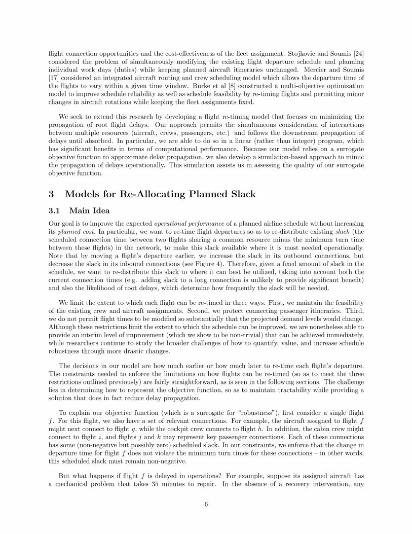
flight connection opportunities and the cost-effectiveness of the fleet assignment. Stojkovic and Soumis [24]considered the problem of simultaneously modifying the existing flight departure schedule and planningindividual work days (duties) while keeping planned aircraft itineraries unchanged. Mercier and Soumis[17] considered an integrated aircraft routing and crew scheduling model which allows the departure time ofthe flights to vary within a given time window. Burke et al [8] constructed a multi-objective optimizationmodel to improve schedule reliability as well as schedule feasibility by re-timing flights and permitting minorchanges in aircraft rotations while keeping the fleet assignments fixed.
We seek to extend this research by developing a flight re-timing model that focuses on minimizing thepropagation of root flight delays. Our approach permits the simultaneous consideration of interactionsbetween multiple resources (aircraft, crews, passengers, etc.) and follows the downstream propagation ofdelays until absorbed. In particular, we are able to do so in a linear (rather than integer) program, whichhas significant benefits in terms of computational performance. Because our model relies on a surrogateobjective function to approximate delay propagation, we also develop a simulation-based approach to mimicthe propagation of delays operationally. This simulation assists us in assessing the quality of our surrogateobjective function.
3 Models for Re-Allocating Planned Slack
3.1 Main Idea
Our goal is to improve the expected operational performance of a planned airline schedule without increasingits planned cost. In particular, we want to re-time flight departures so as to re-distribute existing slack (thescheduled connection time between two flights sharing a common resource minus the minimum turn timebetween these flights) in the network, to make this slack available where it is most needed operationally.Note that by moving a flight’s departure earlier, we increase the slack in its outbound connections, butdecrease the slack in its inbound connections (see Figure 4). Therefore, given a fixed amount of slack in theschedule, we want to re-distribute this slack to where it can best be utilized, taking into account both thecurrent connection times (e.g. adding slack to a long connection is unlikely to provide significant benefit)and also the likelihood of root delays, which determine how frequently the slack will be needed.
We limit the extent to which each flight can be re-timed in three ways. First, we maintain the feasibilityof the existing crew and aircraft assignments. Second, we protect connecting passenger itineraries. Third,we do not permit flight times to be modified so substantially that the projected demand levels would change.Although these restrictions limit the extent to which the schedule can be improved, we are nonetheless able toprovide an interim level of improvement (which we show to be non-trivial) that can be achieved immediately,while researchers continue to study the broader challenges of how to quantify, value, and increase schedulerobustness through more drastic changes.
The decisions in our model are how much earlier or how much later to re-time each flight’s departure.The constraints needed to enforce the limitations on how flights can be re-timed (so as to meet the threerestrictions outlined previously) are fairly straightforward, as is seen in the following sections. The challengelies in determining how to represent the objective function, so as to maintain tractability while providing asolution that does in fact reduce delay propagation.
To explain our objective function (which is a surrogate for “robustness”), first consider a single flightf . For this flight, we also have a set of relevant connections. For example, the aircraft assigned to flight fmight next connect to flight g, while the cockpit crew connects to flight h. In addition, the cabin crew mightconnect to flight i, and flights j and k may represent key passenger connections. Each of these connectionshas some (non-negative but possibly zero) scheduled slack. In our constraints, we enforce that the change indeparture time for flight f does not violate the minimum turn times for these connections – in other words,this scheduled slack must remain non-negative.
But what happens if flight f is delayed in operations? For example, suppose its assigned aircraft hasa mechanical problem that takes 35 minutes to repair. In the absence of a recovery intervention, any
6
available slack will be used to absorb this delay, with the residual delay (the delay beyond the availableslack) propagating to the connecting flights. In our example, if the slack between flights f and g is 40minutes, then flight g will not be delayed, but if the slack between flights f and h is only 20 minutes, thenh will experience a 15 minute departure delay. If we move the departure time of flight f to be 15 minutesearlier, then a 35 minute root delay to flight f will no longer propagate to impact flight h.
As a surrogate objective function, we propose to consider the sum of the impacts of each individual rootdelay as it propagates downstream, weighting these delays by their relative probabilities. There are of courselimitations to this approach. First, we are not considering recovery decisions, which can impact how delayspropagate. Incorporating recovery is a sizeable challenge, largely due to the fact that recovery decisions arenot pre-defined but rather based on individual personnel’s prior experience and intuition. We nonethelesssuggest that incorporating some baseline rules for recovery interventions would be an important extensionof our model to consider. Second, we do not consider the interactions of root delays and, as a result, weover-count propagation. For example suppose that the aircraft of flight f connects to flight g, while the crewof flight h also connects to flight g. When we consider the impact of a root delay to flight f , we may capturea downstream impact on flight g. The same will occur when we consider the impact of a root delay to flighth. In reality, should these two root delays occur concurrently, then their effect on flight g will typicallynot be additive. Of course, this over-counting will occur in both the original schedule and our proposedalternative.
While these limitations will impact the quality of our results, we nonetheless suggest that our surrogatefunction can improve over the existing schedule without increasing planned costs, enabling carriers to seeimmediate improvements in their operational performance while the research community continues to seekways to provide further benefits. To support this hypothesis, we have developed a discrete-event simulationmodel (presented in Section 3.4) to help assess the quality of our proposed solutions.
3.2 Single-Layer Model
We begin by presenting a single-layer model (SLM) for redistributing slack. This model only considers theimpact of disruptions one layer “downstream” - that is, on flights directly connected to the flight experiencingthe root disruption.
We present this model for two reasons. First, it provides a simple framework that will facilitate under-standing of the more complex multi-layer model. Second, as demonstrated in section 4, even this simplemodel can yield non-trivial benefits.
3.2.1 Notation
Sets
F set of flightsA set of all considered connectionsM set of possible delay values (minutes) - here we assume that M is a discrete set
Parameters
k+f ≥ 0 ∀f ∈ F the amount by which the departure time of flight f can be moved later
k−f ≥ 0 ∀f ∈ F the amount by which the departure time of flight f can be moved earlier0 ≤ pm
f ≤ 1 ∀m ∈M , ∀f ∈ F the probability that flight f experiences a root delay of m minutessf1,f2 ≥ 0 ∀(f1, f2) ∈ A the slack between flights f1 and f2 in the original schedule
Decision Variables
7
− k−f ≤ xf ≤ k+f ∀f ∈ F
yf1,f2 ≥ 0 ∀(f1, f2) ∈ Adm
f1,f2≥ 0 ∀(f1, f2) ∈ A, ∀m ∈M
xf is the change in the departure time of flight f . This change is restricted to the specified range[−k−f , k+
f ]. Note that a negative value for x means the flight is shifted earlier and a positive value for xmeans that the flight is shifted later.
yf1,f2 corresponds to the new slack between flights f1 and f2, according to the modified schedule.
dmf1,f2
corresponds to the delay that will propagate from flight f1 to flight f2 in the new schedule if thereis a root delay of m minutes imposed on flight f1.
The objective function (1) of SLM minimizes the expected value of the delay propagation by weightingthe probability of an m-minute delay on flight f1 times its propagation to f2, summed over all flight con-nections (f1, f2) and delay lengths m. [Recall that, in this objective function, we consider only one layer ofpropagation.]
Constraints (2) calculate the new slack (yf1,f2) between two flights. This is the old slack (sf1,f2) minusthe change in the departure of the first flight (xf1), plus the change in the departure of the second flight(xf2). Note, as illustrated in Figure 4, that if flight f1 is moved earlier, then xf1 will have a negative valueand the slack yf1,f2 will therefore increase because we are subtracting this value. Constraints (6) ensure thatthe connection stays feasible, i.e. that the slack remains non-negative.
Constraint sets (3) and (4) calculate how much delay would propagate from flight f1 to its outboundconnection f2 if f1 were to experience a root delay of m minutes. Specifically, the propagated delay is mminus yf1,f2 (the root delay minus the new slack between the flights) unless this is negative, in which casethe delay is zero.
Finally, constraints (5) limit the amount by which flight times can be changed. Note that this is flight-specific and can be used not only to restrict changes so that market share is not impacted, but also torecognize gate limitations, slot restrictions, hourly departures (in which case the time window would bezero), etc. Key passenger itineraries could be protected as well, by placing a lower value on the slack time(y) between two connecting flights.
Claim: The solution to (2)-(6) will yield integer values of x.
8
Linear Programming Formulation
• Constraints:
212121 ,, ffffff xxsy +−=
f1 f2min turn original slack
original schedule
f1 f2min turn original slack
modified schedule
01<fx 0
2>fx
new slack original slack
changes in departure times
Introduction Analysis approach Optimization model ResultsPart IFigure 4: Visualizing constraint (2): In this example, the departure of the first flight is shifted earlier by xf1 (whichis negative) and the departure time of the second flight is pushed forward by xf2 (which is positive). As a result, thenew slack (yf1,f2) equals the old slack (sf1,f2) minus xf1 plus xf2 .
Proof: In order to prove the claim, we need to show that the coefficient matrix presented by (2)-(6) istotally unimodular. In that case, given that all elements in the right-hand-side vector of (2)-(6) are integer,all the extreme points of (2)-(6) will be integer [18].
In order to show that the coefficient matrix defined by (2)-(6) is totally unimodular, it is sufficient toprove that the coefficient matrix corresponding to constraints (2) and (3) – or equivalently, its transpose –is totally unimodular. The constraints (4)-(6) are upper and lower bounds, which do not impact the claim.
We can re-write constraint (3) substituting (2), which yields:
dmf1,f2
≥ m− sf1,f2 + xf1 − xf2 ∀(f1, f2) ∈ A, ∀m ∈M (7)
By transferring the variables to the left-hand-side we get:
dmf1,f2
− xf1 + xf2 ≥ m− sf1,f2 ∀(f1, f2) ∈ A, ∀m ∈M (8)
Here we can see that the coefficient matrix (A) corresponding to constraint (8) has entries (aij) of only-1, 0 and 1. Furthermore, we can partition the columns of this matrix into two sets: C1 includes the columnscorresponding to the d variables and C2 the columns corresponding to the x variables. We see that foreach row of this matrix, the summation of all the coefficients in C1 equals 1 and the summation of all thecoefficients in C2 equals 0. Therefore:
|∑j∈C1
aij −∑j∈C2
aij | ≤ 1 ∀i (9)
Therefore, A′ (the transpose of A) is totally unimodular, and thus A itself is also totally unimodular. �
This claim tells us that it is sufficient to solve SLM as an LP, rather than an IP, while still yieldinginteger departure times. This has significant implications not only for the tractability of the model, but alsofor our ability to extend it to include indirect downstream effects, as we see in the next section.
3.3 Multi-Layer Model
The model presented in section 3.2 only considers the impact of a root delay on the flight’s immediateconnections. Of course, these delayed connections can in turn delay their outbound connections as well ifthere is not enough slack to fully absorb the disruption. In this section, we present a multi-layer model(MLM) in which the downstream propagation of delays continues until they are fully absorbed.
To formulate this model, we must first define the notion of a propagation tree. For each root flight f0 andeach delay value m, the propagation tree represents the set of all downstream flights that could potentially bedelayed as a result of the root delay propagating. Note that because we construct these trees before re-timing
9
the flights, we do not know for sure which flights will receive propagated downstream delays. Therefore thepropagation tree considers the “worst-case” scenario.
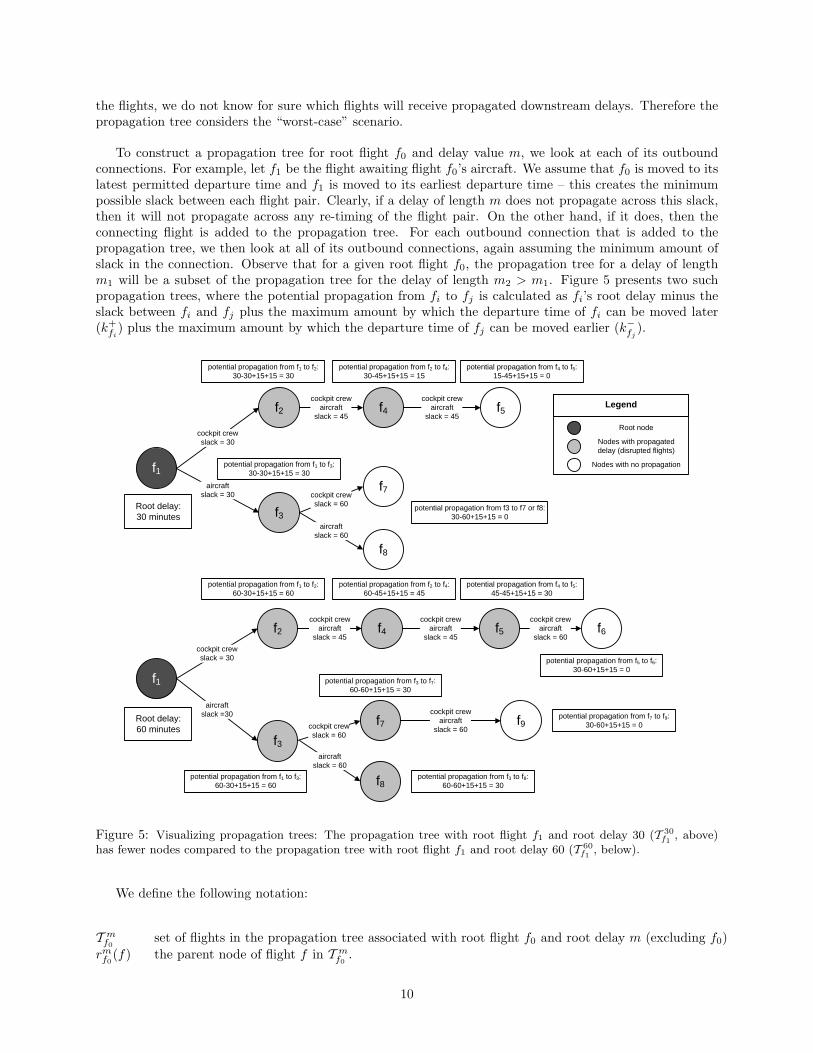
To construct a propagation tree for root flight f0 and delay value m, we look at each of its outboundconnections. For example, let f1 be the flight awaiting flight f0’s aircraft. We assume that f0 is moved to itslatest permitted departure time and f1 is moved to its earliest departure time – this creates the minimumpossible slack between each flight pair. Clearly, if a delay of length m does not propagate across this slack,then it will not propagate across any re-timing of the flight pair. On the other hand, if it does, then theconnecting flight is added to the propagation tree. For each outbound connection that is added to thepropagation tree, we then look at all of its outbound connections, again assuming the minimum amount ofslack in the connection. Observe that for a given root flight f0, the propagation tree for a delay of lengthm1 will be a subset of the propagation tree for the delay of length m2 > m1. Figure 5 presents two suchpropagation trees, where the potential propagation from fi to fj is calculated as fi’s root delay minus theslack between fi and fj plus the maximum amount by which the departure time of fi can be moved later(k+
fi) plus the maximum amount by which the departure time of fj can be moved earlier (k−fj
).
Nodes with no propagation
Nodes with propagated delay (disrupted flights)
Root node
Legend
f1
f2
f3
f4cockpit crewslack = 30
aircraftslack = 30
cockpit crewaircraft
slack = 45f5
cockpit crewaircraft
slack = 45
f1
f2
f3
f4cockpit crewslack = 30
aircraftslack =30
cockpit crewaircraft
slack = 45f5
cockpit crewaircraft
slack = 45f6
cockpit crewaircraft
slack = 60
f8
aircraftslack = 60
f7cockpit crewslack = 60
cockpit crewaircraft
slack = 60f9
f8
aircraftslack = 60
f7cockpit crewslack = 60Root delay:
30 minutes
Root delay: 60 minutes
potential propagation from f1 to f2:30-30+15+15 = 30
potential propagation from f2 to f4:30-45+15+15 = 15
potential propagation from f4 to f5:15-45+15+15 = 0
potential propagation from f1 to f3:30-30+15+15 = 30
potential propagation from f3 to f7 or f8:30-60+15+15 = 0
potential propagation from f1 to f2:60-30+15+15 = 60
potential propagation from f1 to f3:60-30+15+15 = 60
potential propagation from f2 to f4:60-45+15+15 = 45
potential propagation from f4 to f5:45-45+15+15 = 30
potential propagation from f5 to f6:30-60+15+15 = 0
potential propagation from f3 to f7:60-60+15+15 = 30
potential propagation from f3 to f8:60-60+15+15 = 30
potential propagation from f7 to f9:30-60+15+15 = 0
Figure 5: Visualizing propagation trees: The propagation tree with root flight f1 and root delay 30 (T 30f1 , above)
has fewer nodes compared to the propagation tree with root flight f1 and root delay 60 (T 60f1 , below).
We define the following notation:
T mf0
set of flights in the propagation tree associated with root flight f0 and root delay m (excluding f0)rmf0
(f) the parent node of flight f in T mf0
.
10
Based on this notation, we extend the single-layer model to the multi-layer model:
There are two key differences between the single-layer model presented in section 3.2 and this model.First, in the objective (10), we include not only the delay minutes that a root delay of m minutes on flight f0
imposes on f0’s immediate outbound connections, but also the propagated impact on all subsequent flightsin f0’s propagation tree.
Second, constraints (13) enforce the fact that the delay propagated to a flight downstream from the rootdelay will be the amount of delay propagated to its parent minus the amount of slack between these flights.
This model is structurally quite similar to the single-layer model and exhibits the same integrality prop-erty. The main difference is in size. For each flight in any given propagation tree, we have to add both anew variable and a new constraint. As we observe in Section 4, however, the modified formulation remainshighly tractable for networks of a realistic size.
Claim: The solution to (11)-(16) will yield integer values of x.Proof: The proof is similar to the one presented in 3.2. Here we argue that the coefficient matrix presentedby (11)-(13) is totally unimodular. (The constraints (14)-(16) again do not affect the integrality of the xvariables.)
As in the earlier proof, we can re-write constraints (12) by substituting in constraints (11), yielding:
dmf0,f − xf0 + xf ≥ m− sf0,f ∀(f0 ∈ F , f ∈ T m
f0: rm
f0(f) = f0), ∀m ∈M (17)
Note that this constraint, which captures the relationship between the root flight and each of its “chil-dren”, includes one d variable, with coefficient of 1, and two x variables, one with coefficient 1 and one withcoefficient -1.
Next we consider constraint set (13). First, suppose that f is a “grandchild” of f0 – in other words, itsinbound connection is f0’s outbound connection. Then by substituting (11) we get:
dmf0,f ≥ dm
f0,rmf0
(f) − srmf0
(f),f + xrmf0
(f) − xf (18)
and then by substituting (12) we get:
dmf0,f ≥ m− sf0,rm
f0(f) + xf0 − xrm
f0(f) − srm
f0(f),f + xrm
f0(f) − xf (19)
Canceling and moving the variables to the left hand side of the constraint yields:
11
dmf0,f − xf0 + xf ≥ m− sf0,rm
f0(f) − srm
f0(f),f (20)
which again has one d variable with coefficient one and two x variables, one with coefficient 1 and onewith coefficient -1.
More generally, when f is a descendant of f0 in the propagation tree, substitution as above will yield:
dmf0,f − xf0 + xf ≥ m−
∑(f1,f2)∈Pm
f0(f)
sf1,f2 (21)
as all the intermediate x variables cancel, with each intermediate flight on the path from f0 to f playingthe role of both parent and child. [In equation 21, Pm
f0(f) is the set of all arcs (f1, f2) that form the path
from the root node f0 to f in the propagation tree T mf0
.] Again, we see one d variable with coefficient 1 andtwo x variables, one with coefficient 1 and one with coefficient -1.
Thus, using the same partitioning of the columns of the A matrix as the earlier proof, the sufficientcondition for total unimodularity follows directly. �
3.4 Simultaneous Delays Model
The models presented in Sections 3.2 and 3.3 rely on the use of a surrogate objective function to achieverobustness. In particular, objective functions (1) and (10) attempt to minimize the total amount of prop-agated delay in the flight network by looking at how each individual flight propagates delay. The primarylimitation of this approach is that it does not take into account the fact that multiple flight delays may occurin the network simultaneously. As a result, propagated delay will in some cases be estimated inaccurately.Figure 6 presents one such situation.
f0
f1
f2
aircraft
cockpit crew
Root delay: 25 minutes
Root delay: 30 minutes
Individual delays in f0 and f1 each can impact f2
Figure 6: An example of simultaneous root delays where the surrogate objective function overestimates thedelay propagations.
Given flights f0 and f1, both of which are parent (preceding) flights of f2, the objective function includesthe sum of the delays propagated from both f0 and f1. In scenarios where both f0 and f1 experience a rootdelay simultaneously, however, f2’s delay should be the maximum of the two upstream delays, rather thantheir sum.
Conversely, there are occasions where the surrogate objective function underestimates delay. For example,as illustrated in Figure 7, when simultaneous root delays happen consecutively, their overall results can bemore disruptive than what the objective functions in (1) or (10) can estimate. In this figure, individual rootdelays in f0 or f1 are not enough to delay f2. However, when f0 and f1 both experience a thirty-minutedelay, their delays can propagate to cause a ten-minute delay in f2.
12
f0 f1 f2aircraftslack = 20
cockpit crewslack = 30
Root delay: 30 minutes
Root delay: 30 minutes
Individual delays in f0 and f1 do not affect f2, but simultaneous delays in both f0 and f1 will delay f2 by 10 minutes
Figure 7: An example of simultaneous root delays where the surrogate objective function underestimates thedelay propagations.
Given that both the original and the re-timed schedules suffer from these inaccuracies, it is not clearhow the overall reduction in delay propagation is affected. Therefore, we have developed a discrete-eventsimulation model to provide further analysis into the overall effects of this approximation. This enables usto compare how both the original and the optimized schedules perform when multiple flights in the networkincur root delays concurrently.
Note that we assume root delays to be additive, meaning that if a flight has previously incurred apropagated delay, but additionally incurs a root delay, the total departure time is pushed back by the sumof these values. For example, consider the case when a flight is delayed because it is awaiting its (delayed)inbound aircraft. A weather delay or mechanical delay (i.e. a root delay) at the second flight would typicallynot arise until after the incoming aircraft arrived, making these delays additive. On the other hand, whentwo different upstream delays simultaneously affect a flight (e.g. its crew is delayed on one inbound flight andits aircraft delayed on another), then the propagation will be the maximum of the two propagated delays,rather than their sum.
To accurately simulate a given flight network using a discrete-event simulation, we require a source ofrandomness that will be used to determine the amount of root delays incurred by each flight. To model thesedelays, we have generated empirical distributions based on the origin airport of the departing flight, usingactual delay data spanning a 12-month period. Specifically, we filtered out all delays that were propagatedfrom an upstream root disruption. We then clustered the remaining delays by origin station and length ofdisruption. The corresponding probability mass functions were used in both the simulation, to randomlygenerate the initial root delays, and as coefficients in the objective functions of SLM and MLM.
Note that in a given flight schedule, there is no obvious “first flight” – because the schedule is repeating,any particular flight can appear as both the root of one propagation tree and a downstream flight in another.To address this complication, our simulation algorithm employs a recursive strategy that explores all flightsin a given network without requiring a sequential ordering [14].
The delay that a flight experiences consists of two parts – propagated delay (resulting from the needto wait for delayed upstream resources such as cockpit crews, cabin crews and aircraft) and root delay(associated with the flight itself, such as a weather delay). The propagated delay is computed by taking themaximum delay across all of the inbound resources, then adding this to the root delay.
To compute the total propagated delay in the network, we first initialize all flights in the network to havea propagated delay of zero and a root delay of zero. After this initialization stage, the propagation algorithmproceeds by executing the following steps for each flight in the network.
We pick an arbitrary flight in the network to process and call upon the random delay generator to providea root delay for this particular flight. If this root delay is non-zero, we update the departure time of thecurrent flight to be the sum of the (current value of the) propagated delay and this additional root delay.We then consider all outbound connections from this particular flight. For each connection, we determinehow much (if any) of the current flight’s delay would propagate to this child. We then check whether this
13
propagated delay is larger than the connecting flight’s current propagated delay. If it is, we update theconnecting flight’s propagated delay. Next, we add this to the connecting flight’s root delay (which will bezero if that flight hasn’t been processed yet) to determine its new departure time. Finally, we recursivelyuse this new departure time to update the propagated delay of its outbound connections, repeating until aflight delay does not propagate.
This process repeats until all flights in the network have been processed and therefore exposed to thepossibility of incurring a root delay. Through the recursive nature of the algorithm, we are guaranteed toexplore every flight and every propagation tree, updating them with the appropriate amount of propagateddelay.
4 Computational Experiments
The objectives of our computational experiments were three-fold. First, we wanted to assess the run-timeperformance of our models and determine their tractability. Second, we wanted to evaluate the extent towhich minor changes in flight times could impact the potential for delays to propagate – would the optimizedschedule have significantly less delay propagation than the original schedule? Third, we wanted to usesimulation to assess the accuracy of our surrogate objective function, i.e. our metric for delay propagation.When multiple delays are allowed to occur simultaneously, as is the case in reality, does the our new schedulestill show improved performance over the original schedule?
Our computational experiments were conducted using data provided by a major U.S. carrier offering over500 flights per day. We considered two different dates in 2007. For each of these dates, we were given theflight schedule, cockpit crew schedules, and aircraft rotations. Thus, we were able to consider propagationof delays associated with incoming aircraft and cockpit crews. [We did not include delays associated withcabin crews or connecting passengers, due to lack of data.]
As a default, we assumed that each flight was allowed to be moved up to fifteen minutes earlier orfifteen minutes later than its original departure time. Note that, in theory, this could impact crew costs andfeasibility. For example, if a duty were currently at its maximum allowed elapsed time and we moved thedeparture time of the first flight of the duty earlier and/or moved the departure time of the last flight of theduty later, then we would violate the elapsed time limit.
To account for this, we considered four different variations. In the first and most restrictive case, weassumed that the first flight of any duty could not be moved earlier and the last flight of any duty couldnot be moved later. This greatly limits the flexibility of the network. In both of the data sets considered,most of the flights are either the first or last flights of their duty, and thus only about twenty-five percent ofthe flights were allowed to move freely. Furthermore, this overly restricts the system: in a duty whose costis dominated by flying time, increasing the elapsed time by stretching the first and last flights slightly mayhave no impact on cost, and the feasibility of the duty may be unchanged as well.
Therefore, we considered three additional instances, each progressively less restrictive. In these, the firstand last flights of the duty were only allowed to change by five minutes, by ten minutes, or by the samefifteen minutes as all other flights in the network.
All code was implemented and run on an Intelr Pentiumr D 3.20 GHz CPU architecture using the C++programming language. The optimization models were developed using CPLEX/Concert Technology andsolved using CPLEX 11.0 solver.
14
4.1 Goal 1 – Tractability
Table 2 shows the size and run time of each problem instance solved. The first column of this table indicateswhich of the two data sets is being considered. The second column indicates the restriction on first and lastflights in a duty (note that all other flights have a ± fifteen minute time window in all instances). The thirdcolumn indicates whether the single-layer or multi-layer model is being used. The fourth, fifth, and sixthcolumns give the size of the model (in number of constraints, number of variables and number of nonzeroelements) and the final column gives the run time (in seconds).
Table 2: Size of the instances and their corresponding run times.
Note that all run times are less than 10 seconds, suggesting that there is no computational limitationon either model. Although the model size increases substantially when moving from the single-layer modelto the multi-layer model, the fact that the problem can be solved as an LP implies that tractability is notsacrificed when using the more accurate model.
Finally, these results suggest that even if a significant number of additional connections were considered(e.g. incorporating cabin crews, key passenger itineraries, etc), run times would remain tractable.
4.2 Goal 2 – Impact
Our second goal was to evaluate the potential improvements in delay propagation to be gained by re-timingflights slightly. First, we began by computing two estimates of the propagated delay of the original schedules– one using the objective function from the single-layer model and one using the more accurate objectivefunction from the multi-layer model. We then optimized the original schedules twice, once using each of thetwo objective functions. Again, for each of these solutions, we computed both the SLM and MLM objectiveestimates of delay propagation.
Table 3 presents these results. The first column specifies which of the two data sets is being analyzed.The second column indicates how many minutes the first/last flights of a duty are allowed to change. Thenext three columns present the objective function value of the original, single-layer optimal, and multi-layeroptimal schedules relative to the single-layer objective function. For the optimized schedules, (n%) indicatesthe percent improvement over the original schedule, relative to the single-layer objective function. Likewise,the following three columns represent the multi-layer objective function applied to the three schedules.
Observe that, as expected, the amount of propagation is larger for all scenarios when multiple layers ofpropagation are taken into account. In addition, the single-layer optimal solution of course performs better
Table 3: Reduction in the objective function (potential delay propagation) – comparing different schedules
under the single-layer objective, while the multi-layer optimal solution performs better under the multi-layeroptimization.
It is interesting to note that there is not a dramatic difference between the single- and the multi- layerschedules in their performance under the multi-layer objective function. This is presumably due to the factthat the delays dissipate fairly quickly and thus the immediate outbound connection plays a dominant role.[See [3] for an empirical analysis of the characteristics of propagation trees.] Therefore, minimizing the firstlayer of delays will capture much of the possible benefits.
Finally, we observe that flight re-timing can have substantial improvements on the delay propagation,ranging from approximately 5 percent for the most tightly restricted instances to approximately 50 percentfor the least restricted instances. Of course, there are several caveats that must accompany these results.First, we did not take into account the delay propagation associated with cabin crews or any passengeritineraries for which the second flight of the itinerary would be “held” for connecting passengers (these couldeasily be incorporated, given available data, and would have little impact on run times). It is not clear whatimpact these additions would have on the quality of the optimal solutions, as the changes would impact boththe original and the modified schedules. Second, we have not taken into account recovery decisions, whichagain will affect propagation within both the original and the optimized schedules. Finally, we re-iteratethat our surrogate objective function over-counts propagation because it considers each delay one at a time.We address this limitation through the use of a discrete-event simulation model in the next section.
4.3 Goal 3 – Validity
In order to better assess the impact of the fact that the surrogate objective function does not incorporate theconcurrency of delays in our optimization model, we simulated each of the schedules (the original scheduleand the re-timed schedules based on the single-layer and multi-layer models) using the same probabilitydistribution functions for the root delays as in the optimization models.
The results are summarized in Table 4. The first two columns describe the instance. The next threecolumns give the ratio of the expected amount of delay propagation (in minutes), as estimated by 2000replications of the simulation model, divided by the value of the surrogate objective function under theoriginal or re-timed schedule.
As expected, the simulated values differ from the surrogate values. However, the ratio is fairly consistent,suggesting that the impact of ignoring concurrent delays has comparable impact on both the original and there-timed schedules. Thus, it is not surprising that the simulated value of the re-timed schedules still demon-strates a significant improvement over the simulated value of the original schedule. Table 5 demonstratesthis. The first two columns describe the instance. The next three columns give the expected amount of delaypropagation (in minutes), as estimated by the simulation model, for each of the three schedules. Columnsfour and five also provide the relative improvement over the original schedule. Although these improvements
Table 5: Reduction in the delay propagation (simulation results) – comparing different schedules
are lower than the surrogate objective values, they nonetheless demonstrate a substantial opportunity forreduction in delay propagation through minor flight re-timings.
4.4 Discussion
We conclude this section with a few final observations.
First, we note that changing flight times can make key passenger itineraries infeasible by decreasing theconnection time between them beyond that which is feasible for a passenger to connect. Such itineraries canbe protected by adding constraints of the form:
yf1,f2 = sf1,f2 − xf1 + xf2 (22)yf1,f2 ≥ 0 (23)
which says that, for a protected itinerary (f1, f2), the time between the scheduled arrival of flight f1
and the scheduled departure of flight f2 must not decrease below the minimum passenger connection time.Observe, however, that we do not include delay propagation from flight f1 to flight f2 in the model, becausewe do not assume that flights are delayed to await connecting passengers.
Second, we observe that – as with any model – the re-timing solutions that result from our models willonly be starting points, which will need to be fine-tuned before implementation. In particular, although the0-minute model may be overly restrictive in terms of maintaining the current crew costs and feasibility, the15-minute model may result in some crew violations. These violations would have to be corrected manually,but we suggest that substantial benefits can still remain even after these modifications.
Third, to partially reduce this post-processing, we suggest that one way to reduce crew infeasibilitieswould be to identify the largest amount by which the length of the duty could increase without violating
17
elapsed time limits and/or changing cost the dominant cost from the flight time to the elapsed time. Then,for each duty, a constraint of form:
−xf ′ + xf ′′ ≤ emax − e (24)
could be used to ensure that the length of the duty not increase beyond this limit. In the above constraint,f ′ and f ′′ are the first and the last flights of a duty respectively, e is the elapsed time of that particular duty,and emax is the maximum elapsed time in a duty.
5 Conclusions and Future Research
Airline delays have significant negative impact on airline costs, passenger convenience and productivity, andthe environment. One major cause of delay is the down-stream propagation of initial delays to subsequentflights. This issue is exacerbated by the fact that slack is undesirable from a planning perspective, asit “wastes” costly resources, but is critical from an operational perspective, as it can be used to absorbdisruptions and prevent their propagation.
Addressing operational concerns in the planning process can be quite challenging, however. First, metricsfor evaluating the operational performance of a planned schedule must be developed. Second, cost functionsmust be developed to trade-off planned and (anticipated) operational costs. Finally, these cost functionsmust be incorporated in an already-challenging planning process. In particular, because delay propagationspans across multiple resources, schedule design, fleeting, crew scheduling, and maintenance routing mustall be considered concurrently.
As an intermediate measure to partially decrease the propagation of delay while these other challengingtopics are studied by the research community, we propose to modify flight departure times within theframework of an existing airline plan. By re-allocating the existing slack to those flight connections thatare most prone to delay propagation, we can reduce downstream impacts without changing planned crewor fleeting costs and without changing revenue projections. Our computational results show significantopportunities for improvement without any increase in planned costs.
Future research in this area of course includes the three issues raised above – metrics for evaluatingthe robustness of a planned schedule, cost functions for computing the trade-off between planned costs andanticipated operational costs, and methods for incorporating these cost functions in the planning process.In the shorter time horizon, our research could be expanded by more explicitly addressing correlationsbetween different root delays. Finally, we are interested in including recovery decisions (e.g. canceling flights,swapping aircraft, and calling in reserve crews) in our model to capture their impacts on the operationalperformance of a planned schedule under disruptions.
Acknowledgments:
We gratefully acknowledge the financial support of the Alfred P. Sloan Foundation Industry Studies Programand the MIT Global Airline Industry Program.
References
[1] J. Abara. Applying integer linear programming to the fleet assignment problem. Interfaces, 19:20–38,1989.
[2] A. Abdelghany, G. Ekollu, R. Narasimhan, and K. Abdelghany. A proactive crew recovery decision sup-port tool for commercial airlines during irregular operations. Annals of Operations Research, 127:309–331, 2004.
18
[3] S. AhmadBeygi, A.M. Cohn, Y. Guan, and P. Belobaba. Analysis of the potential for delaypropagation in passenger airline networks. Technical report, 2007. http://www.umich.edu/ amy-cohn/PAPERS/proptreefinal.pdf, to appear in Journal of Air Transport Management.
[4] C. Barnhart, A. Cohn, E. Johnson, D. Klabjan, G. Nemhauser, and P. Vance. Handbook of Transporta-tion Science, chapter Airline Crew Scheduling. Kluwer’s International Series, 2003.
[5] C. Barnhart and K. Talluri. Design and Operation of Civil and Environmental Engineering Systems,chapter Airline Operations Research, pages 435–469. John Wiley and Sons, New York, 1997.
[6] M. Berge. Timetable optimization: Formulation, solution approaches, and computational issues. pages341–357, 1994. AGIFORS proceedings, Zandvcort, The Netherlands.
[7] S. Bratu and C. Barnhart. Flight operations recovery - new approaches considering passenger recovery.Journal of Scheduling, 9:279–298, 2006.
[8] E.K. Burke, P. De Causmaecker, G. De Maere, J. Mulder, M. Paelinck, and G. Vanden Berghe. A multi-objective approach for robust airline scheduling. Computers and Operations Research, (to appear), 2007.
[9] M. Clarke, L. Lettovsky, and B. Smith. Handbook of Airline Operations, chapter The Development ofthe Airline Operations Control Center, pages 131–147. Aviation Week, 2000.
[10] B. Fuhr. Robust flight scheduling - an analytic approach to performance evaluation and optimization.Technical report, 2007. Clausthal University of Technology - Lufthansa Airlines.
[11] D. Klabjan, E. L. Johnson, and G. L. Nemhauser. Airline crew scheduling with regularity. TransportationScience, 35(4):359–374, 2001.
[12] N. Kohl, A. Larsen, J. Larsen, A. Ross, and S. Tiourine. Airline disruption management perspectives,experiences and outlook. Journal of Air Transport Management, 13:149–162, 2007.
[13] S. Lan, J.P. Clarke, and C. Barnhart. Planning for robust airline operations: Optimizing aircraftroutings and flight departure times to minimize passenger disruptions. Transportation Science, 40(1),2006.
[14] M. Lapp, S. AhmadBeygi, A.M. Cohn, and O. Tsimhoni. A recursion-based approach to simulatingairline schedule robustness. Technical report, 2008. To be submitted to proceedings of the 2008 WinterSimulation Conference.
[15] L. Lettovsky, E.L. Johnson, and G.L. Nemhauser. Airline crew recovery. Transportation Science,34(4):337–348, 2000.
[16] A. Levin. Scheduling and fleet routing models for transportation systems. Transportation Science,5:232–255, 1971.
[17] A. Mercier and F. Soumis. An integrated aircraft routing, crew scheduling and flight retiming model.Computers and Operations Research, 34(8):2251–2265, 2007.
[18] George L. Nemhauser and Laurence A. Wolsey. Integer and combinatorial optimization. Wiley-Interscience, New York, NY, USA, 1988.
[19] B. Rexing, C. Barnhart, T. Kniker, A. Jarrah, and N. Krishnamurthy. Airline fleet assignment withtime windows. Transportation Science, 34(1):120, 2000.
[20] J. Rosenberger, E. Johnson, and G. Nemhauser. A robust fleet-assignment model with hub isolationand short cycles. Transportation Science, 38(3):357–369, 2004.
[21] J.M. Rosenberger, A.J. Schaefer, D. Goldsman, A.J. Kleywegt, E.L. Johnson, and G.L. Nemhauser. Astochastic model of airline operations. Transportation Science, 36(4):357–377, 2002.
19
[22] A. Schaefer, E. Johnson, J. Kleywegt, and G. Nemhauser. Airline crew scheduling under uncertainty.Transportation Science, 39(3):340–348, 2005.
[23] G. Stojkovic, F. Soumis, J. Desrosiers, and M. M. Solomon. An optimization model for a real-time flightscheduling problem. Transportation Research Part A, 36:779–788, 2002.
[24] M. Stojkovic and F. Soumis. An optimization model for the simultaneous operational flight and pilotscheduling problem. Management Science, 47(9):1290–1305, 2001.
[25] S. Yan and D.H. Yang. A decision support framework for handling schedule perturbation. TransportationResearch Part B, 30(6):405–419, 1996.
[26] J. Yen and J. Birge. A stochastic programming approach to the airline crew scheduling problem.Transportation Science, 40(1):3–14, 2006.
[27] G. Yu and X. Qi. Disruption management: Framework, Models and Applications. World ScientificPublishing, 2004.