Page 1
Eotvos Lorand Science University
Faculty of sience
Gabor Damasdi
Mathematics BSc
Slope number of graphs with bounded degree
BSc thesis
Supervisor: Domotor Palvolgyi, assistant professor
Department of Computer Sience
Budapest, 2015.
Page 3
Contents
1 Introduction 1
1.1 Know results . . . . . . . . . . . . . . . . . . . . . . . . . . . . . . . 2
1.2 Definitions . . . . . . . . . . . . . . . . . . . . . . . . . . . . . . . . . 3
2 Lemmas and ideas 4
3 Proof of main theorem 11
3.1 Triangle-free graphs . . . . . . . . . . . . . . . . . . . . . . . . . . . . 11
3.2 Graphs with triangles . . . . . . . . . . . . . . . . . . . . . . . . . . . 20
3.2.1 Non-contractible triangle . . . . . . . . . . . . . . . . . . . . . 20
3.2.2 Contractible triangle . . . . . . . . . . . . . . . . . . . . . . . 22
4 Open questions and remarks 23
Page 4
Acknowledgements
I would like to thank my supervisor, Domotor Palvolgyi for introducing me to this
topic and helping me through my work. Without his continuous support, this work
would not have been possible.
Page 5
1 Introduction
Drawing of graphs is a popular topic in mathematics. It has practical applications in
engineering, network research, traffic control, computer networks and it also raises
interesting theoretical questions.
A straight-line drawing of a graph is a layout of its vertices in the plane such that
the vertices are distinct points, and the line segments connecting the corresponding
point pairs are not passing through any other point that represents a vertex. In this
thesis we will only consider straight-line drawings. These drawings can be measured
in different ways.
The crossing number of a drawing is the number of pairs of edges that cross each
other. If a drawing with no crossings exists, we call the graph planar. Kuratowski
gave a nice characterization of planar graphs: A finite graph is planar if and only if
it does not contain a subgraph that is a subdivision of K5 or K3,3 [6].
Angular resolution is a measure of the sharpest angle in a graph drawing. If
a graph has vertices with high degree, then it necessarily will have small angular
resolution. Malitz and Papakostas showed that every planar graph with maximum
degree d has a planar drawing whose angular resolution is at worst an exponential
function of d, independent of the number of vertices in the graph [7].
The slope number of a graph G is the smallest number k such that G has a
straight-line drawing using k distinct edge slopes. It was introduced by Wade and
Chu [10], who showed that the slope number of Kn is n if n > 2. It is hard to tell
the slope number of a graph in general. It has been shown that it is NP-complete
to decide whether a graph has slope number two [3].
Figure 1: A drawing of the hypercube using 4 slopes.
1
Page 6
We might be able to determine the slope number if we restrict our graph in some
way. Obviously, if the maximal degree is d, then the slope number is at least d2, so
it is natural to consider graphs with bounded degree. We can also ask the slope
number for trees, planar graphs, Hamiltonian graphs, etc.
The main topic of my thesis is the slope number of graphs. I will prove some
new result concerning 3-regular Hamiltonian graphs.
1.1 Know results
The slope number of graphs with bounded degree is an active topic in mathematics.
Let us say that the degrees are bounded by d. In recent years the following results
have been established.
Theorem 1.1 (Barat et al. [1], Pach and Palvolgyi [9]). If d > 4, then the slope
number can be arbitrary large.
Theorem 1.2 (Keszegh et al. [5]). If d = 3, then the slope number is at most 5.
Theorem 1.3 (Mukkamala and Palvogyi [8]). If d = 3, then the slope number is at
most 4, and we can always use the horizontal, vertical and two diagonal slopes.
Unfortunately this last theorem had some mistakes in its proof. The idea of the
proof is to draw parts of the graphs first and then build up the drawing from the
smaller parts. This idea only worked for graphs with at least 18 vertices. For most
of the graphs with less then 18 vertices they used the following theorem.
Theorem 1.4 (Engelstein [2]). For all 3-regular 3-connected Hamiltonian graphs
the slope number is at most 4.
This theorem only states that 3-regular, 3-connected Hamiltonian graphs can be
drawn with some set of four distinct slopes. It does not prove that it can be done
with the horizontal, vertical and two diagonal slopes.
To fix this we will improve these results on 3-regular Hamiltonian graphs with
the following theorem.
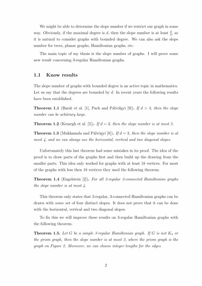
Theorem 1.5. Let G be a simple 3-regular Hamiltonian graph. If G is not K4 or
the prism graph, then the slope number is at most 3, where the prism graph is the
graph on Figure 2. Moreover, we can choose integer lengths for the edges.
2
Page 7
Figure 2: The prism graph.
In this theorem we did not pick a set of slopes to be used in the drawing. The
reason for this is the following.
Lemma 1.6. If we can draw a graph with 3 different slopes, then we can draw it
with any set of 3 different slopes.
Proof. There is an affine transformation that takes the original slopes into the new
ones. This transformation can be used on the drawing. Since a set of parallel lines
remain parallel after an affine transformation, the new drawing is a straight-line
drawing with the required set of slopes.
1.2 Definitions
From Lemma 1.6 we see that we can choose 3 arbitrary slopes for our proofs. Al-
though Theorem 1.3 requires the horizontal, vertical and diagonal slopes, we will
always use the slopes that are defined by 3th roots of unity. So the slopes are 0,√
3
and −√
3, and we call these the basic slopes.
If it leads to no confusion, we will make no distinction between the vertices and the
corresponding points in the drawing, and similarly between the edges and segments.
There are drawings of Hamiltonian graphs in the thesis. In most of them the black
edges are representing the Hamiltonian cycle and the rest of the edges are red.
Let the following names define the 6th roots of unity:
• VEast: (1, 0)
• VNorthEast: (12,√32
)
• VNorthWest: (−12,√32
)
• VWest: (−1, 0)
• VSouthWest: (−12, −√3
2)
• VSouthEast: (12, −√3
2)
We say that point A lies east to B if A-B is a positive constant times VEast. Similarly
we use the other defined directions.
3
Page 8
2 Lemmas and ideas
In this section we will prove some useful lemmas and explain some ideas. We use
them later to prove Theorem 1.5.
Definition 2.1. Let G be a 3-regular Hamiltonian graph. We can divide the edges
of G into two groups. The first group is the edges of the Hamiltonian cycle. We
will call these cycle edges. Since G is 3-regular, the rest of the edges form a perfect
matching. We will call these matching edges. Define the pair of a vertex as the
other vertex of the matching edge it is on.
The main idea behind our proof is the following lemma.
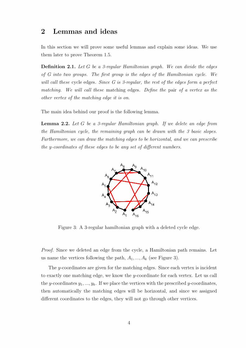
Lemma 2.2. Let G be a 3-regular Hamiltonian graph. If we delete an edge from
the Hamiltonian cycle, the remaining graph can be drawn with the 3 basic slopes.
Furthermore, we can draw the matching edges to be horizontal, and we can prescribe
the y-coordinates of these edges to be any set of different numbers.
Figure 3: A 3-regular hamiltonian graph with a deleted cycle edge.
Proof. Since we deleted an edge from the cycle, a Hamiltonian path remains. Let
us name the vertices following the path, A1, ..., Ak (see Figure 3).
The y-coordinates are given for the matching edges. Since each vertex is incident
to exactly one matching edge, we know the y-coordinate for each vertex. Let us call
the y-coordinates y1, ..., yk. If we place the vertices with the prescribed y-coordinates,
then automatically the matching edges will be horizontal, and since we assigned
different coordinates to the edges, they will not go through other vertices.
4
Page 9
We will calculate x1, ..., xk in a recursive way. x1 is arbitrary. If i > 1, then
xi = xi−1 + |(yi − yi−1)| ·1√3
(2.1)
From the equation we see that the slope of the edge AiAi+1 is either√
3 or
−√
3. This means that all edges have correct slopes. We need to check that the
edges do not go through vertices. We have seen that the matching edges do not
cause problems. The x-coordinates of the vertices are monotone increasing along
the Hamiltonian path, so the cycle edges are also good.
Figure 4: A solution provided by Lemma 2.2.
Remark 2.3. It is important to note that if the y-coordinates we choose are multiples
of√
3, then the lengths of the edges are integers.
Proof. From Equation (2.1) we can see that if the y-coordinates are multiples of√
3,
then xi − xi−1 is integer for every i. From this it follows that xi − xj is integer for
every i and j. So the horizontal edges have integer length.
The length of AiAi+1 is
√(xi − xi+1)2 + (yi − yi+1)2 =
√((yi − yi+1) ·
1√3
)2 + (yi − yi+1)2 = 2 · |yi − yi+1|√3
Since the y-coordinates are multiples of√
3, this is an integer. Hence all of the
edges have integer length. It is easy to see that we draw the graph onto a triangular
grid.
5
Page 10
Remark 2.4. Another important observation is that if we follow the Hamiltionian
path in the drawing, we always go in either southeast or northeast direction. In other
words, for every i < j pair there are bi,j and ci,j non-negative numbers such that
Aj = Ai + bi,j · VNorthEast + ci,j · VSouthEast.
Proof. If j = i + 1, this is trivial. Ai+1 has strictly bigger x-coordinate than Ai
therefore Ai has to be either to the southeast or to the northeast of Ai.
If j > i+ 1, then Aj −Ai = (Aj −Aj−1) + (Aj−1−Aj−2) + ...+ (Ai+1−Ai). We
have seen that the parts of the sum are good, so the sum is also good.
We can also see that bi,j = bi,i+1 + bi+1,i+2 + ... + bj−1,j and similarly ci,j =
ci,i+1 + ci+1,i+2 + ... + cj−1,j.
As we can see, Lemma 2.2 almost proves Theorem 1.5. The only problem is the
deleted edge. It might have a wrong slope and it can also go through other vertices.
Unfortunately it is not too easy to fix this problem. We will divide the graphs into
groups and solve them in different ways. The following lemmas and ideas will help
us with some of the cases.
Definition 2.5. Let G be a 3-regular graph which contains a triangle. We can delete
the triangle from the graph and replace it with a vertex, and then connect the vertex
to the vertices the triangle was connected to. We will call this process the contraction
of the triangle (see Figure 5).
Figure 5: Contraction of a triangle.
6
Page 11
Definition 2.6. Let G be a 3-regular graph which contains a triangle. Each vertex
of the triangle is incident to an edge which is not in the triangle. If these 3 edges
are independent, then we call the triangle contractible. If they are not, we will call
it non-contractible.
The meaning behind the definition is the following. It will be useful to us to
contract the triangle into one point. If the three edges are independent, then the
new graph we get is simple, but if they are not independent, it will not be simple,
since there will be a multiple edge.
Lemma 2.7. Contraction of a contractible triangle preserves 3-regularity and Hamil-
tonicity.
Proof. The degrees of the unchanged vertices remain 3. The new vertex has degree
3 since the triangle has 3 vertices and each vertex adds an edge to the new vertex.
So the new graph is 3-regular.
The three independent edges connected to the triangle form a cut, so the Hamil-
tonian cycle contains exactly two of them. If we contract the triangle, these two
edges will meet in the new vertex. Hence we lose two edges from the Hamiltonian
cycle, but the rest of the edges of the cycle will from a Hamiltonian cycle in the new
graph.
Definition 2.8. If we have a drawing, the vertices can be divided into groups. Two
vertices are in the same group if the edges incident to them are in the same direction.
We will call this property the type of the vertex.
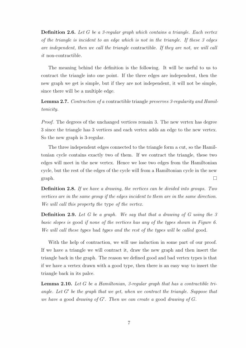
Definition 2.9. Let G be a graph. We say that that a drawing of G using the 3
basic slopes is good if none of the vertices has any of the types shown in Figure 6.
We will call these types bad types and the rest of the types will be called good.
With the help of contraction, we will use induction in some part of our proof.
If we have a triangle we will contract it, draw the new graph and then insert the
triangle back in the graph. The reason we defined good and bad vertex types is that
if we have a vertex drawn with a good type, then there is an easy way to insert the
triangle back in its palce.
Lemma 2.10. Let G be a Hamiltonian, 3-regular graph that has a contractible tri-
angle. Let G′ be the graph that we get, when we contract the triangle. Suppose that
we have a good drawing of G′. Then we can create a good drawing of G.
7
Page 12
Figure 6: Bad vertex types.
Proof. We will modify the drawing of G′ to get a drawing for G. Let A be the vertex
that we made from the triangle. Since it is a good drawing, there are two edges that
are connected to A and the angle of their slopes is 60◦. We make a new vertex on
both of these edges at a fixed distance from A. We connect these new vertices. Let
B and C denote the two new vertex. Since BAC∠ = 60◦ and AB = AC, the ABC
triangle is equilateral. This means that the new BC edge has a good slope. We have
to check that BC does not go through other vertices. Since the graph has finitely
many vertices, A has a small neighbourhood that does not contain other vertices.
We can choose the length of AB to be so small, that the ABC triangle will be in
the neighbourhood. So the BC edge cannot go through other vertices.
Figure 7: Inflation of a triangle.
It is easy to see that the new drawing is good. The type of the old vertices did
not change. The two new vertices are part of an equilateral triangle, so they cannot
have a bad type.
If the edges in the original drawing had integer length they can be integer in the
new drawing too. If we chose the length of AB to be rational, all of the edges will
8
Page 13
have rational length. Therefore, we can simply enlarge the drawing by an integer
factor to receive integer lengths.
Since Lemma 2.10 requires a good drawing, we will modify Theorem 1.5 to be slightly
stronger:
Theorem 2.11. Let G be a simple 3-regular Hamiltonian graph. If G is not K4
or the prism graph, then the slope number is at most 3. Moreover, we can choose
integer lengths for the edges, and we can also make it a good drawing.
Remark 2.12. It is worth to note that Lemma 2.2 gives us a good drawing.
Proof. The Ai−1Ai edge meets the AiAi+1 edge either in 60◦ or 180◦. In either case
Ai cannot have a bad type. We only have two edges at A0 and Ak, but that two
meet in 60◦ so even if we extend the drawing, they will have a good type.
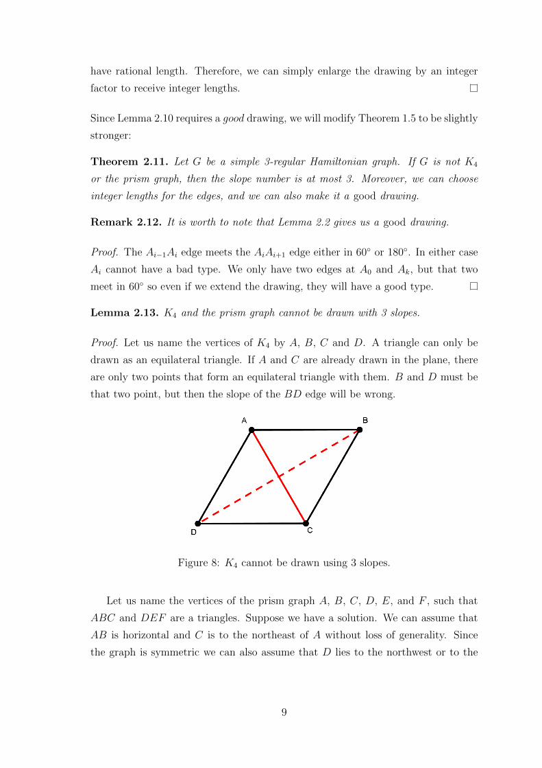
Lemma 2.13. K4 and the prism graph cannot be drawn with 3 slopes.
Proof. Let us name the vertices of K4 by A, B, C and D. A triangle can only be
drawn as an equilateral triangle. If A and C are already drawn in the plane, there
are only two points that form an equilateral triangle with them. B and D must be
that two point, but then the slope of the BD edge will be wrong.
Figure 8: K4 cannot be drawn using 3 slopes.
Let us name the vertices of the prism graph A, B, C, D, E, and F , such that
ABC and DEF are a triangles. Suppose we have a solution. We can assume that
AB is horizontal and C is to the northeast of A without loss of generality. Since
the graph is symmetric we can also assume that D lies to the northwest or to the
9
Page 14
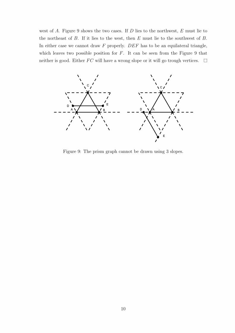
west of A. Figure 9 shows the two cases. If D lies to the northwest, E must lie to
the northeast of B. If it lies to the west, then E must lie to the southwest of B.
In either case we cannot draw F properly. DEF has to be an equilateral triangle,
which leaves two possible position for F . It can be seen from the Figure 9 that
neither is good. Either FC will have a wrong slope or it will go trough vertices.
Figure 9: The prism graph cannot be drawn using 3 slopes.
10
Page 15
3 Proof of main theorem
As we have seen in Lemma 2.2, we have an algorithm which is almost good. To
prove Theorem 2.11 we will consider different cases. In each case we will use Lemma
2.2 to draw most of the graph, and draw some vertices in a different way.
3.1 Triangle-free graphs
First we will prove that Theorem 2.11 holds for triangle-free graphs. If we have a
triangle, we must draw it as an equilateral triangle. It is a big constraint so we will
deal with them in a different way.
The following lemma proves that we can find a special part of the graph if it is
triangle-free. We will draw this part differently.
Lemma 3.1. Let G be a 3-regular, Hamiltonian, triangle-free graph, with at least 10
vertices. We can find a Hamiltonian cycle and A,B,C,D,E, F,X, Y vertices with
the following properties:
1. A,B,C,D,E, F,X and Y are distinct.
2. A,B,C,D,E, F are consecutive vertices on the Hamiltonian cycle in this or-
der.
3. CY and DX are matching edges.
4. The order of C,D,X, Y along the cycle is CDXY .
Figure 10: The required configuration.
11
Page 16
Proof. If we have already chosen C and D, and CD is a cycle edge, we can trivially
choose A,B,E, F,X, Y to satisfy condition 1, 2 and 3. We choose A, B, E and F to
be the vertices that precede and follow C and D on the cycle. We choose X and Y
to be the pairs of C and D. Since the graph is triangle-free, these will be different
vertices. Therefore, the main goal is to satisfy condition 4.
Let us pick a Hamiltonian cycle. There are two cases to consider.
First case: Each vertex is adjacent to the opposite vertex in the cycle. In this
case we will use another Hamiltonian cycle instead. We can simply switch two
opposite cycle edges with two matching edges as Figure 11 shows. We can use the
second case on the new Hamiltonian cycle.
Figure 11: Redefining the Hamiltonian cycle.
Second case: Not every vertex is adjacent to the opposite vertex. We can pick a
matching edge that divides the Hamiltonian cycle into two parts that are not equal
in size. Denote by P2, P3, ...Pr the vertices of the bigger part, starting from P1 and
going along the cycle. Similarly denote by Q2, Q3, .., Qs the vertices in the smaller
(see Figure 12). We pick the smallest l such that Pl is connected to Pj by a matching
edge. There is an l like that because there are more Pi’s than Qi’s. Denote by Qk
the pair of Pl−1. We will choose the vertices the following way: C = Pl, D = Pl−1
and as we have seen, we can chose A,B,E, F,X, Y to satisfy condition 1, 2 and 3.
Let us check condition 4. Pl and Pj divides the cycle into two part. Qk is in the
same part as Pl−1, since in the other part there are only Pi’s. So the order of Pl,
Pl−1, Pj and Qk is appropriate.
We will even need a slightly stronger lemma.
12
Page 17
Figure 12: The labeling of the graph.
Lemma 3.2. Let G be a 3-regular, Hamiltonian, triangle-free graph, with at least 10
vertices. We can find a Hamiltonian cycle and A,B,C,D,E, F,X, Y vertices with
the following properties:
1. A,B,C,D,E, F,X and Y are distinct.
2. A,B,C,D,E, F are consecutive vertices on the Hamiltonian cycle in this or-
der.
3. CY and DX are matching edges.
4. The order of C,D,X, Y along the cycle is CDXY .
5. At least one of AE or BF is not a matching edge.
Proof. As in the previous lemma, we will choose C and D, which will give us
A,B,E, F,X, Y , and we will have to check condition 4 and 5.
First we choose the vertices according to the previous lemma. We know that the
first four condition is met, so we only have consider the case when the fifth is not
(Figure 13). In this case continue the naming of the vertices with G, H and I along
the cycle. G, H and I can be the same as X or Y , but they are not A, B, C, D, E
or F , since we have at least 10 vertices. We will choose new vertices to satisfy this
lemma, and to avoid confusion we will mark them with an apostrophe.
First case: If G 6= X then we choose C ′ = F and D′ = G, and the rest to satisfy
condition 1, 2 and 3.
B and F divides the cycle into two parts. One part only consists C, D and E,
so if condition 4 is not true, then G is adj to one of them. G is not X, Y or A which
means its pair cannot be C, D or E.
13
Page 18
Figure 13: Condition 5 of Lemma 3.2 is not met in this graph.
B′ = E and it is adjacent to A. A is not I, so B′F ′ is not a matching edge. So
condition 5 is met.
Second case: If G = X, then we choose C ′ = G and D′ = H, and the rest to
satisfy condition 1, 2 and 3.
H cannot be adjacent to E or F since they are adjacent to A and B. This means
that condition 4 is met.
If condition 5 would not be true, A and B would come after H on the cycle.
It would mean that we only have 8 vertices. Since we have at least 10, it is not
possible.
Now we can prove Theorem 2.11 for triangle-free graphs. We will use the graph
in Figure 14 to illustrate the process.
Figure 14: A triangle-free graph with A,B,C,D,E,F,X,Y chosen.
We use the Lemma 3.2 to choose A,B,C,D,E, F,X, Y vertices. Let A1, A2, ...Al
be the vertices between A and Y . Let B1, B2, ...Bm be the vertices between Y and
14
Page 19
X. Let C1, C2, ...Cn be the vertices between X and F (see Figure 14). This is a
point where we use condition 4 from Lemma 3.2. If the order of CDXY would not
be right, the A-s, B-s and C-s would not be distinct vertices.
First we will draw the graph using Lemma 2.2. The deleted edge is CD. We
need to assign y-coordinates to the matching edges.
Lemma 3.3. We can choose the y-coordinates to satisfy the following properties:
1. CY and DX have smaller y-coordinate than the rest.
2. B has smaller y-coordinate than A.
3. E has smaller y-coordinate than F .
4. All y-coordinates are multiples of√
3.
5. The y-coordinate of CY and DX are consecutive multiples of√
3
Proof. We will assign the 0,√
3, 2 ·√
3, ... numbers to the edges. CY will have 0 and
DX will have√
3. From condition 5 in Lemma 3.2 we know that either AE or BF
is not a matching edge. The reason to require condition 5 in Lemma 3.2 was to be
able to satisfy condition 2 and 3 at the same time in this lemma.
If AE is not a matching edge, then the edge coming from E receives 2 ·√
3
and the edge coming from B receives 3 ·√
3. The rest of the coordinates can be
assigned arbitrarily. Since AE is not an edge, this means that A will have a bigger y-
coordinate than B. Condition 3 is also true since the only two smaller y-coordinates
than E has, were assigned to the CY and DX edges.
If BF is not a matching edge, then the edge coming from B receives 2 ·√
3 and
the edge coming from E receives 3 ·√
3. The rest of the coordinates can be assigned
arbitrarily. Since BF is not an edge, this means that F will have a bigger y-
coordinate than E. Condition 3 is also true since the only two smaller y-coordinates
than B has, were assigned to the CY and DX edges.
With the combination of Lemma 2.2 and Lemma 3.3 we get a drawing of the
graph using 3 slopes (see Figure 15). We only have to fix the missing CD edge. We
delete the C and D vertices and redraw them differently. We draw a ray from B
in southeast direction. We have seen in Remark 2.4 that all of the vertices can be
written as B + c1 ·VNorthEast + c2 ·VSouthEast where c1 and c2 are non-negative. Since
15
Page 20
Figure 15: The drawing after the first stage.
A has a bigger y-coordinate than B, c1 is never zero. It means that none of the
vertices can lie southeast to B. We draw a ray from Y in the direction of southwest.
Since only X can have smaller y-coordinate than Y , none of the vertices but X can
be on this ray. From condition 4 in Lemma 3.2 we know that X was drawn later
then Y , so it has a bigger x-coordinate. Therefore, not even X can lie on this ray.
We place C in the intersection of the two rays. In a symmetric way we place D
southeast of X and southwest of E.
Figure 16: The drawing after redrawing C and D.
As we can see in Figure 16 the CD edge still can have a wrong slope but since
C and D are lower the rest of the vertices, it will not go trough any vertices. We
will make the CD edge horizontal. Without loss of generality we can assume that
16
Page 21
C has a bigger y-coordinate than D. Let d denote the difference of the y-coordinate
of C and D. Let m denote the number of vertices between X and Y . We have to
consider three cases.
First case: m > 0. In this case B1 exists and there is an edge between Y and
B1. Since Y has smaller y-coordinate than B1, B1 lies to the northeast of Y .
We will fix the drawing by translating some of its parts. Since translation pre-
serves directions, the edges inside the translated parts will remain good.
Let us translate C and Y by d · 2√3· VSouthWest. This moves C downwards with
d, so this will make CD horizontal. Also C remains southwest of Y and Y remains
southwest of B1. We translate B, A, A1, ... Al by d· 2√3·VWest. Since it is a horizontal
translation the matching edges will remain good. C will still be southeast of B since
B − C changed with d · (VSouthWest − VWest) · 2√3
= d · VSouthEast · 2√3. Similarly Y
remains southeast of Al.
We also have to check that the drawings are good. By remark 2.12 we know that
the vertices are correct except for C, D, X and Y . BCY ∠ = 60◦, XDE∠ = 60◦,
AlY B∠ = 60◦, BmXC1∠ = 60◦, so they are good too.
Figure 17: The completed drawing.
Second case: m = 0 and d =√
3, so X and Y are neighbours. If X has a bigger
y-coordinate than Y , everything works like in the first case. The only difference is
that Y is adjacent to X instead of B1.
If X has smaller y-coordinate we translate Y and C by 2 · VSouthWest and we
translate B, A, A1, ... Al by 2 · VWest. Similarly to the previous case everything
17
Page 22
remains good, we just have to check Y X and CD. From condition 5 in Lemma
3.3 we know that the y-coordinate of Y and X are consecutive multiples of√
3.
Since Y has a bigger y-coordinate, translating it by 2 · VSouthWest will turn Y X into
horizontal. Since d =√
3, we know that the y coordinate of C is bigger than the
y-coordinate of D by√
3. We translated C by 2 · VSouthWest, therefore CD will be
horizontal too.
We now have a drawing with 3 slopes but it is not a good drawing. The type of
X and Y is bad. We can easily fix this:
We translate C, Y , B, A, A1, ... Al by 3 · VEast. Notice that there are only
horizontal edges between C, Y , B, A, A1, ... Al and the rest of the vertices. Since it
is a horizontal translation, the slopes of the edges will not change. We only have to
check that none of the edges go trough any of the vertices. The structure of the two
parts does not change. The only possible problem is that a vertex form one part of
the graph moves onto an edge in the other part of the graph. It is easy to see from
the x-coordinates of the vertices that this cannot happen.
The new drawing is a good drawing. The type of the vertices did not change
except for X and Y . Now XY Al∠ = 60◦ and Y XC1∠ = 60◦, therefore X and Y
have a good type now.
Figure 18: An example to the second case.
18
Page 23
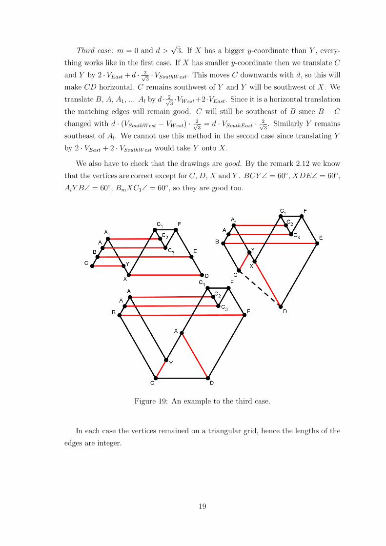
Third case: m = 0 and d >√
3. If X has a bigger y-coordinate than Y , every-
thing works like in the first case. If X has smaller y-coordinate then we translate C
and Y by 2 · VEast + d · 2√3· VSouthWest. This moves C downwards with d, so this will
make CD horizontal. C remains southwest of Y and Y will be southwest of X. We
translate B, A, A1, ... Al by d· 2√3·VWest+2·VEast. Since it is a horizontal translation
the matching edges will remain good. C will still be southeast of B since B − C
changed with d · (VSouthWest − VWest) · 2√3
= d · VSouthEast · 2√3. Similarly Y remains
southeast of Al. We cannot use this method in the second case since translating Y
by 2 · VEast + 2 · VSouthWest would take Y onto X.
We also have to check that the drawings are good. By the remark 2.12 we know
that the vertices are correct except for C, D, X and Y . BCY ∠ = 60◦, XDE∠ = 60◦,
AlY B∠ = 60◦, BmXC1∠ = 60◦, so they are good too.
Figure 19: An example to the third case.
In each case the vertices remained on a triangular grid, hence the lengths of the
edges are integer.
19
Page 24
3.2 Graphs with triangles
3.2.1 Non-contractible triangle
Suppose that we have a triangle but it is non-contractible. By definition the three
edges that are connected to the triangle are not independent. There are two cases,
first if these three edges have a common vertex. It can only happen if the graph is
K4. As we have seen K4 cannot be drawn with 3 slopes.
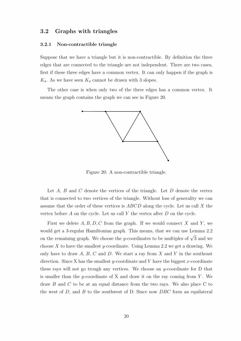
The other case is when only two of the three edges has a common vertex. It
means the graph contains the graph we can see in Figure 20.
Figure 20: A non-contractible triangle.
Let A, B and C denote the vertices of the triangle. Let D denote the vertex
that is connected to two vertices of the triangle. Without loss of generality we can
assume that the order of these vertices is ABCD along the cycle. Let us call X the
vertex before A on the cycle. Let us call Y the vertex after D on the cycle.
First we delete A,B,D,C from the graph. If we would connect X and Y , we
would get a 3-regular Hamiltonian graph. This means, that we can use Lemma 2.2
on the remaining graph. We choose the y-coordinates to be multiples of√
3 and we
choose X to have the smallest y-coordinate. Using Lemma 2.2 we get a drawing. We
only have to draw A, B, C and D. We start a ray from X and Y in the southeast
direction. Since X has the smallest y-coordinate and Y have the biggest x-coordinate
these rays will not go trough any vertices. We choose an y-coordinate for D that
is smaller than the y-coordinate of X and draw it on the ray coming from Y . We
draw B and C to be at an equal distance from the two rays. We also place C to
the west of D, and B to the southwest of D. Since now DBC form an equilateral
20
Page 25
Figure 21: A graph with a non-contractible triangle.
triangle whose altitude is half of the distance between the rays, we can place A on
the ray coming from X to form an equilateral triangle with B and C. This gives us
an appropriate drawing.
Figure 22: The drawing of Figure 21.
We have to check that the drawing is good. By remark 2.12 we only have to
check A, B, C and D. Since each part of a triangle, they cannot have a bad type.
If choose the y-coordinate of D to be a multiple of√
3 then the length of the
edges will be integer.
21
Page 26
3.2.2 Contractible triangle
We are going to use induction on the number of the vertices. Since the graph is
3-regular we only have to consider graphs with an even number of vertices.
Lemma 3.4. Theorem 2.11 holds if the number of the vertices is 6 or 8.
Proof. There is only one 3-regular connected simple graph with 6 vertices that is
not the prism graph. There are only five 3-regular connected simple graphs with
8 vertices [11]. All of them are Hamiltonian. Their drawings can be seen in the
following figure.
Figure 23: 3-regular connected simple graphs with 6 or 8 vertices.
Notice that all of the drawings are good, and the edges can have integer lengths.
Suppose the graph has more than 8 vertices. Since we have a contractible trian-
gle, we can contract it into one point. By Lemma 2.10 we know that it is enough
to draw the smaller graph. By induction we know that if there is a non-contractible
triangle, then we have a good drawing for it. If there is no contractible triangle, we
can use the other parts of the proof to get a good drawing.
A graph is either triangle-free or it contains a triangle. We proved both cases,
hence Theorem 2.11 is true. Theorem 2.11 is stronger than Theorem 1.5, therefore
we proved that one too.
22
Page 27
4 Open questions and remarks
We have shown that we can have integer lengths for the edges. It is easy to see that
we can have integer coordinates instead. If we have a drawing that uses the basic
slopes and the edges have integer lengths, we can just multiply the y-coordinates by1√3. Since the y-coordinates were multiples of
√3, this will make them integer. We
have seen previously that the difference of the x-coordinates are integers, thus we
can translate the drawing horizontally to get integer coordinates.
We proved that 3-regular Hamiltonian graphs can be drawn with 3 slopes. An
interesting question is to determine which graphs can be drawn with 3 slopes? How
important is Hamiltonicity?
Lemma 4.1. The following graph cannot be drawn using 3 slopes.
Figure 24: This graph cannot be drawn using 3 slopes.
Proof. Suppose we have a drawing. ABC is a triangle in the graph so they will form
an equilateral triangle in the drawing. ACD is also a triangle, so they will also form
an equilateral triangle. Since there are only two points in the plane that forms an
equilateral triangle with A and C, one on each side of the AC line, the points D
and B will lie on different side of the AC line. E is connected to B, but it cannot
lie on BA or BC. There is 4 other possible half-line where we can place E. Since
none of those intersect the AC line, B and E will be on the same side of the AC
line. Similarly E and D will be on the same side of the AC line. It is not possible
since D and B must lie on different side of the AC line.
From this it follows that every graph that contains this graph as a subgraph
cannot be drawn using 3 slopes.
23
Page 28
Conjecture 4.2. A 3-regular graph can be drawn using 3 slopes if it is not the prism
graph or K4, and it does not contain the graph in Figure 24 as a subgraph.
Let d denote the maximal degree of the graph. One of the most interesting open
question in this topic is the case of d = 4. Theorem 1.1 solves the d > 4 case and
1.3 solves the d = 3 case. Nothing is know in the d = 4 case.
24
Page 29
References
[1] Barat, J.; Matousek, J.; Wood, D. R. Bounded-Degree Graphs have Arbitrarily
Large Geometric Thickness, The Electronic Journal of Combinatorics, 13, (2006)
[2] Engelstein, M. Drawing graphs with few slopes. Intel Competition for high school
students, (2005)
[3] Formann, M.; Hagerup, T.; Haralambides, J.; Kaufmann, M.; Leighton, F. T.;
Symvonis, A.; Welzl, E.; Woeginger, G. Drawing graphs in the plane with high
resolution, SIAM Journal on Computing, 22 (5): 1035–1052, (1993)
[4] Garg, A.; Tamassia, R. On the computational complexity of upward and recti-
linear planarity testing, SIAM Journal on Computing, 31 (2): 601–625, (2001)
[5] Keszegh, B.; Pach, J.; Palvolgyi, D; Toth, G. Drawing cubic graphs with at most
five slopes. Computational Geometry: Theory and Applications, 40(2):138–147,
(2008)
[6] Kuratowski, K. Sur le probleme des courbes gauches en topologie, Fund. Math.,
15: 271–283, (1930)
[7] Malitz, S.; Papakostas, A. On the angular resolution of planar graphs. SIAM J.
Discrete Math., 7(2): 172–183, (1994)
[8] Mukkamala, P.; Palvolgyi, D. Drawing cubic graphs with the four basic slopes.
Graph Drawing 2011, volume 7034: 254–265, (2012)
[9] Pach, J.; Palvolgyi, D. Bounded-degree graphs can have arbitrarily large slope
numbers. Electronic Journal of Combinatorics, 13(1):1–4, (2006)
[10] Wade, G. A.; Chu, J. H. Drawability of complete graphs using a minimal slope
set, The Computer J., 37: 139–142, (1994)
[11] http://en.wikipedia.org/wiki/Table of simple cubic graphs
25