Small Angle Scattering and Large Scale Structures H. Frielinghaus This document has been published in Manuel Angst, Thomas Brückel, Dieter Richter, Reiner Zorn (Eds.): Scattering Methods for Condensed Matter Research: Towards Novel Applications at Future Sources Lecture Notes of the 43rd IFF Spring School 2012 Schriften des Forschungszentrums Jülich / Reihe Schlüsseltechnologien / Key Tech- nologies, Vol. 33 JCNS, PGI, ICS, IAS Forschungszentrum Jülich GmbH, JCNS, PGI, ICS, IAS, 2012 ISBN: 978-3-89336-759-7 All rights reserved.
Transcript
Small Angle Scattering and Large Scale Structures
H. Frielinghaus
This document has been published in
Manuel Angst, Thomas Brückel, Dieter Richter, Reiner Zorn (Eds.):Scattering Methods for Condensed Matter Research: Towards Novel Applications atFuture SourcesLecture Notes of the 43rd IFF Spring School 2012Schriften des Forschungszentrums Jülich / Reihe Schlüsseltechnologien / Key Tech-nologies, Vol. 33JCNS, PGI, ICS, IASForschungszentrum Jülich GmbH, JCNS, PGI, ICS, IAS, 2012ISBN: 978-3-89336-759-7All rights reserved.
D 1 Small Angle Scattering and Large ScaleStructures1
3 Small Angle X-ray Scattering 203.1 Contrast variation using anomalous small angle x-ray scattering . . . . . . . . 22
4 Comparison of SANS and SAXS 23
A Guinier Scattering 26
1Lecture Notes of the43rd IFF Spring School “Scattering Methods for Condensed MatterResearch: TowardsNovel Applications at Future Sources” (ForschungszentrumJulich, 2012). All rights reserved.
D1.2 H. Frielinghaus
1 Introduction
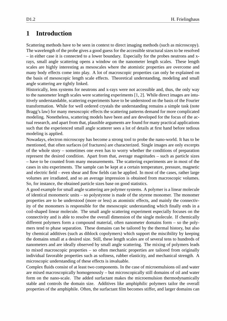
Scattering methods have to be seen in context to direct imaging methods (such as microscopy).The wavelength of the probe gives a good guess for the accessible structural sizes to be resolved– in either case it is connected to a lower boundary. Especially for the probes neutrons and x-rays, small angle scattering opens a window on the nanometerlength scales. These lengthscales are highly interesting as mesoscales where the atomistic properties are overcome andmany body effects come into play. A lot of macroscopic properties can only be explained onthe basis of mesoscopic length scale effects. Theoretical understanding, modeling and smallangle scattering are tightly linked.Historically, lens systems for neutrons and x-rays were notaccessible and, thus, the only wayto the nanometer length scales were scattering experiments[1, 2]. While direct images are intu-itively understandable, scattering experiments have to beunderstood on the basis of the Fouriertransformation. While for well ordered crystals the understanding remains a simple task (noteBragg’s law) for many mesoscopic effects the scattering patterns demand for more complicatedmodeling. Nonetheless, scattering models have been and aredeveloped for the focus of the ac-tual research, and apart from that, plausible arguments arefound for many practical applicationssuch that the experienced small angle scatterer sees a lot ofdetails at first hand before tediousmodeling is applied.Nowadays, electron microscopy has become a strong tool to probe the nano-world. It has to bementioned, that often surfaces (of fractures) are characterized. Single images are only excerptsof the whole story – sometimes one even has to worry whether the conditions of preparationrepresent the desired condition. Apart from that, average magnitudes – such as particle sizes– have to be counted from many measurements. The scattering experiments are in most of thecases in situ experiments. The sample can be kept at a certaintemperature, pressure, magneticand electric field – even shear and flow fields can be applied. Inmost of the cases, rather largevolumes are irradiated, and so an average impression is obtained from macroscopic volumes.So, for instance, the obtained particle sizes base on good statistics.A good example for small angle scattering are polymer systems. A polymer is a linear moleculeof identical monomeric units – so polystyrene is made of the styrene monomer. The monomerproperties are to be understood (more or less) as atomistic effects, and mainly the connectiv-ity of the monomers is responsible for the mesoscopic understanding which finally ends in acoil-shaped linear molecule. The small angle scattering experiment especially focuses on theconnectivity and is able to resolve the overall dimension ofthe single molecule. If chemicallydifferent polymers form a compound material, often nanometer domains form – so the poly-mers tend to phase separation. These domains can be tailoredby the thermal history, but alsoby chemical additives (such as diblock copolymers) which support the miscibility by keepingthe domains small at a desired size. Still, these length scales are of several tens to hundreds ofnanometers and are ideally observed by small angle scattering. The mixing of polymers leadsto mixed macroscopic properties – so often mechanic properties are tailored from originallyindividual favorable properties such as softness, rubber elasticity, and mechanical strength. Amicroscopic understanding of these effects is invaluable.Complex fluids consist of at least two components. In the case of microemulsions oil and waterare mixed macroscopically homogenously – but microscopically still domains of oil and waterform on the nano-scale. The added surfactant makes the microemulsion thermodynamicallystable and controls the domain size. Additives like amphiphilic polymers tailor the overallproperties of the amphiphile. Often, the surfactant film becomes stiffer, and larger domains can
Small Angle Scattering D1.3
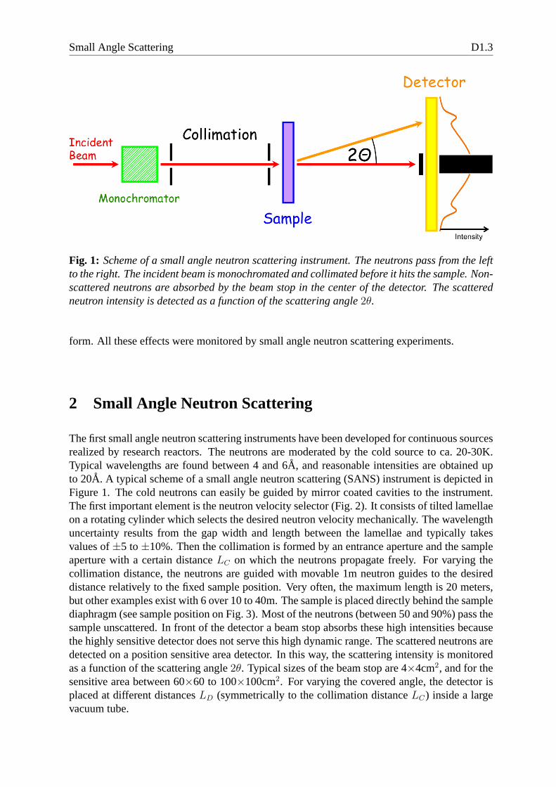
Fig. 1: Scheme of a small angle neutron scattering instrument. The neutrons pass from the leftto the right. The incident beam is monochromated and collimated before it hits the sample. Non-scattered neutrons are absorbed by the beam stop in the center of the detector. The scatteredneutron intensity is detected as a function of the scattering angle2θ.
form. All these effects were monitored by small angle neutron scattering experiments.
2 Small Angle Neutron Scattering
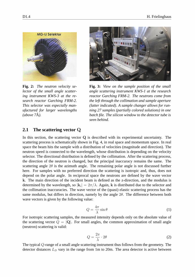
The first small angle neutron scattering instruments have been developed for continuous sourcesrealized by research reactors. The neutrons are moderated by the cold source to ca. 20-30K.Typical wavelengths are found between 4 and 6A, and reasonable intensities are obtained upto 20A. A typical scheme of a small angle neutron scattering (SANS) instrument is depicted inFigure 1. The cold neutrons can easily be guided by mirror coated cavities to the instrument.The first important element is the neutron velocity selector(Fig. 2). It consists of tilted lamellaeon a rotating cylinder which selects the desired neutron velocity mechanically. The wavelengthuncertainty results from the gap width and length between the lamellae and typically takesvalues of±5 to±10%. Then the collimation is formed by an entrance aperture and the sampleaperture with a certain distanceLC on which the neutrons propagate freely. For varying thecollimation distance, the neutrons are guided with movable1m neutron guides to the desireddistance relatively to the fixed sample position. Very often, the maximum length is 20 meters,but other examples exist with 6 over 10 to 40m. The sample is placed directly behind the samplediaphragm (see sample position on Fig. 3). Most of the neutrons (between 50 and 90%) pass thesample unscattered. In front of the detector a beam stop absorbs these high intensities becausethe highly sensitive detector does not serve this high dynamic range. The scattered neutrons aredetected on a position sensitive area detector. In this way,the scattering intensity is monitoredas a function of the scattering angle2θ. Typical sizes of the beam stop are 4×4cm2, and for thesensitive area between 60×60 to 100×100cm2. For varying the covered angle, the detector isplaced at different distancesLD (symmetrically to the collimation distanceLC) inside a largevacuum tube.
D1.4 H. Frielinghaus
Fig. 2: The neutron velocity se-lector of the small angle scatter-ing instrument KWS-3 at the re-search reactor Garching FRM-2.This selector was especially man-ufactured for larger wavelengths(above 7A).
Fig. 3: View on the sample position of the smallangle scattering instrument KWS-1 at the researchreactor Garching FRM-2. The neutrons come fromthe left through the collimation and sample aperture(latter indicated). A sample changer allows for run-ning 27 samples (partially colored solutions) in onebatch file. The silicon window to the detector tube isseen behind.
2.1 The scattering vector Q
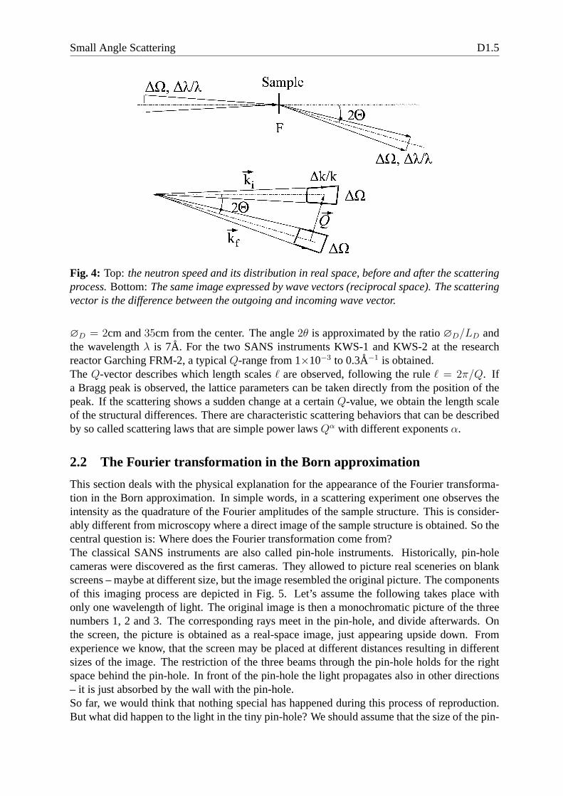
In this section, the scattering vectorQ is described with its experimental uncertainty. Thescattering process is schematically shown in Fig. 4, in realspace and momentum space. In realspace the beam hits the sample with a distribution of velocities (magnitude and direction). Theneutron speed is connected to the wavelength, whose distribution is depending on the velocityselector. The directional distribution is defined by the collimation. After the scattering process,the direction of the neutron is changed, but the principal inaccuracy remains the same. Thescattering angle2θ is the azimuth angle. The remaining polar angle is not discussed furtherhere. For samples with no preferred direction the scattering is isotropic and, thus, does notdepend on the polar angle. In reciprocal space the neutrons are defined by the wave vectork. The main direction of the incident beam is defined as the z-direction, and the modulus isdetermined by the wavelength, so|ki| = 2π/λ. Again,k is distributed due to the selector andthe collimation inaccuracies. The wave vector of the (quasi) elastic scattering process has thesame modulus, but differs in direction, namely by the angle2θ. The difference between bothwave vectors is given by the following value:
Q =4π
λsin θ (1)
For isotropic scattering samples, the measured intensity depends only on the absolute value ofthe scattering vectorQ = |Q|. For small angles, the common approximation of small angle(neutron) scattering is valid:
Q =2π
λ· 2θ (2)
The typicalQ-range of a small angle scattering instrument thus follows from the geometry. Thedetector distancesLD vary in the range from 1m to 20m. The area detector is active between
Small Angle Scattering D1.5
Fig. 4: Top: the neutron speed and its distribution in real space, beforeand after the scatteringprocess.Bottom:The same image expressed by wave vectors (reciprocal space).The scatteringvector is the difference between the outgoing and incoming wave vector.
∅D = 2cm and35cm from the center. The angle2θ is approximated by the ratio∅D/LD andthe wavelengthλ is 7A. For the two SANS instruments KWS-1 and KWS-2 at the researchreactor Garching FRM-2, a typicalQ-range from 1×10⁻³ to 0.3A−1 is obtained.TheQ-vector describes which length scalesℓ are observed, following the ruleℓ = 2π/Q. Ifa Bragg peak is observed, the lattice parameters can be taken directly from the position of thepeak. If the scattering shows a sudden change at a certainQ-value, we obtain the length scaleof the structural differences. There are characteristic scattering behaviors that can be describedby so called scattering laws that are simple power lawsQα with different exponentsα.
2.2 The Fourier transformation in the Born approximation
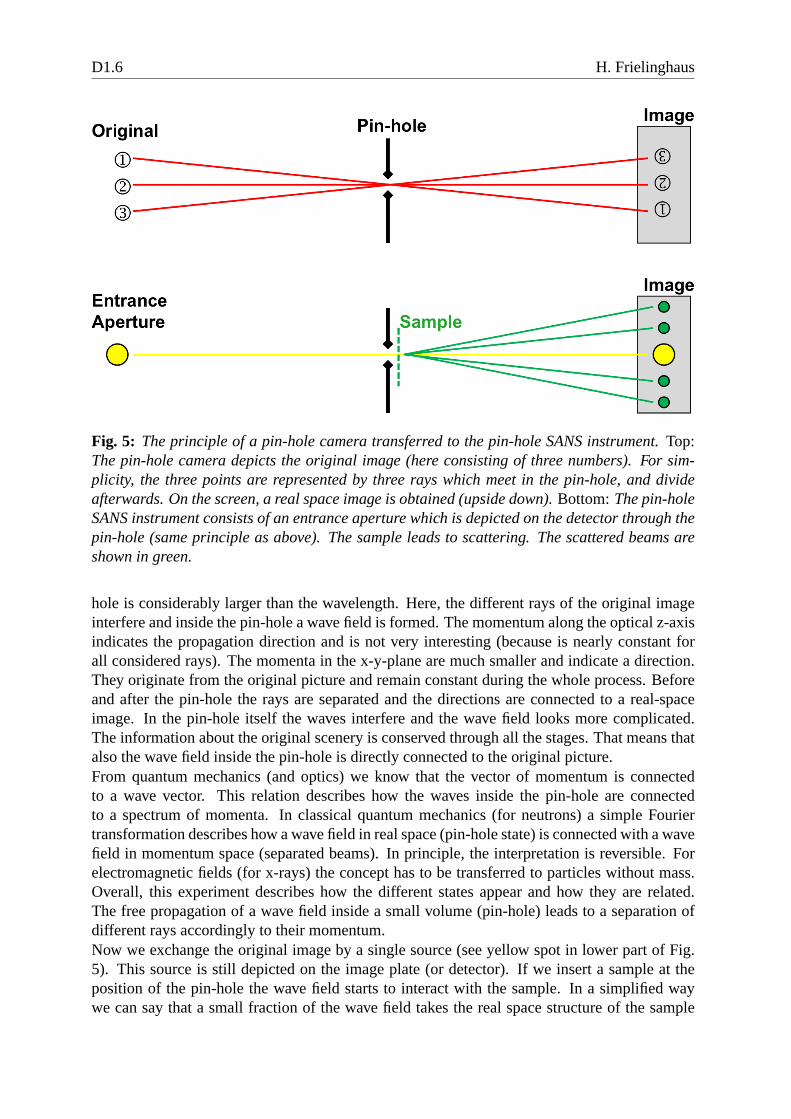
This section deals with the physical explanation for the appearance of the Fourier transforma-tion in the Born approximation. In simple words, in a scattering experiment one observes theintensity as the quadrature of the Fourier amplitudes of thesample structure. This is consider-ably different from microscopy where a direct image of the sample structure is obtained. So thecentral question is: Where does the Fourier transformation come from?The classical SANS instruments are also called pin-hole instruments. Historically, pin-holecameras were discovered as the first cameras. They allowed topicture real sceneries on blankscreens – maybe at different size, but the image resembled the original picture. The componentsof this imaging process are depicted in Fig. 5. Let’s assume the following takes place withonly one wavelength of light. The original image is then a monochromatic picture of the threenumbers 1, 2 and 3. The corresponding rays meet in the pin-hole, and divide afterwards. Onthe screen, the picture is obtained as a real-space image, just appearing upside down. Fromexperience we know, that the screen may be placed at different distances resulting in differentsizes of the image. The restriction of the three beams through the pin-hole holds for the rightspace behind the pin-hole. In front of the pin-hole the lightpropagates also in other directions– it is just absorbed by the wall with the pin-hole.So far, we would think that nothing special has happened during this process of reproduction.But what did happen to the light in the tiny pin-hole? We shouldassume that the size of the pin-
D1.6 H. Frielinghaus
Fig. 5: The principle of a pin-hole camera transferred to the pin-hole SANS instrument.Top:The pin-hole camera depicts the original image (here consisting of three numbers). For sim-plicity, the three points are represented by three rays whichmeet in the pin-hole, and divideafterwards. On the screen, a real space image is obtained (upside down).Bottom:The pin-holeSANS instrument consists of an entrance aperture which is depicted on the detector through thepin-hole (same principle as above). The sample leads to scattering. The scattered beams areshown in green.
hole is considerably larger than the wavelength. Here, the different rays of the original imageinterfere and inside the pin-hole a wave field is formed. The momentum along the optical z-axisindicates the propagation direction and is not very interesting (because is nearly constant forall considered rays). The momenta in the x-y-plane are much smaller and indicate a direction.They originate from the original picture and remain constant during the whole process. Beforeand after the pin-hole the rays are separated and the directions are connected to a real-spaceimage. In the pin-hole itself the waves interfere and the wave field looks more complicated.The information about the original scenery is conserved through all the stages. That means thatalso the wave field inside the pin-hole is directly connectedto the original picture.From quantum mechanics (and optics) we know that the vector of momentum is connectedto a wave vector. This relation describes how the waves inside the pin-hole are connectedto a spectrum of momenta. In classical quantum mechanics (for neutrons) a simple Fouriertransformation describes how a wave field in real space (pin-hole state) is connected with a wavefield in momentum space (separated beams). In principle, theinterpretation is reversible. Forelectromagnetic fields (for x-rays) the concept has to be transferred to particles without mass.Overall, this experiment describes how the different states appear and how they are related.The free propagation of a wave field inside a small volume (pin-hole) leads to a separation ofdifferent rays accordingly to their momentum.Now we exchange the original image by a single source (see yellow spot in lower part of Fig.5). This source is still depicted on the image plate (or detector). If we insert a sample at theposition of the pin-hole the wave field starts to interact with the sample. In a simplified waywe can say that a small fraction of the wave field takes the realspace structure of the sample
Small Angle Scattering D1.7
Fig. 6: How a Fourier transformation is obtained with refractive lenses. The real space struc-ture in the focus of the lens is transferred to differently directed beams. The focusing lens isconcave since for neutrons the refractive index is smaller than 1.
while the major fraction passes the sample without interaction. This small fraction of the wavefield resulting from the interaction propagates freely towards the image plate and generatesa scattering pattern. As we have learned, the momenta present in the small fraction of thewave field give rise to the separation of single rays. So the real space image of the sampleleads to a Fourier transformed image on the detector. This isthe explanation how the Fouriertransformation appears in a scattering experiment – so thisis a simplified motivation for theBorn approximation. A similar result was found by Fraunhoferfor the diffraction of light atsmall apertures. Here, the aperture forms the wave field (at the pin-hole) and the far field isconnected to the Fourier transformation of the aperture shape.Later we will see that the size of wave field packages at the pin-hole is given by the coherencevolume. The scattering appears independently from such small sub-volumes and is a simplesuperposition.
2.3 Remarks on focusing SAS instruments
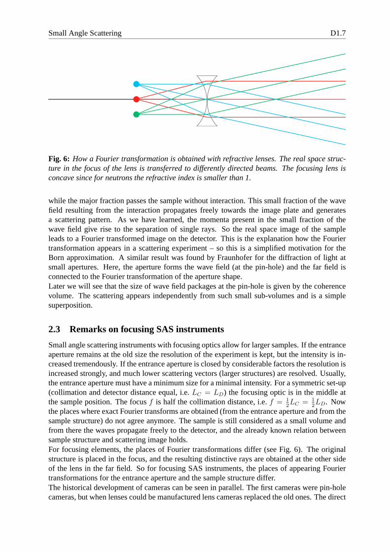
Small angle scattering instruments with focusing optics allow for larger samples. If the entranceaperture remains at the old size the resolution of the experiment is kept, but the intensity is in-creased tremendously. If the entrance aperture is closed byconsiderable factors the resolution isincreased strongly, and much lower scattering vectors (larger structures) are resolved. Usually,the entrance aperture must have a minimum size for a minimal intensity. For a symmetric set-up(collimation and detector distance equal, i.e.LC = LD) the focusing optic is in the middle atthe sample position. The focusf is half the collimation distance, i.e.f = 1
2LC = 1
2LD. Now
the places where exact Fourier transforms are obtained (from the entrance aperture and from thesample structure) do not agree anymore. The sample is still considered as a small volume andfrom there the waves propagate freely to the detector, and the already known relation betweensample structure and scattering image holds.For focusing elements, the places of Fourier transformations differ (see Fig. 6). The originalstructure is placed in the focus, and the resulting distinctive rays are obtained at the other sideof the lens in the far field. So for focusing SAS instruments, the places of appearing Fouriertransformations for the entrance aperture and the sample structure differ.The historical development of cameras can be seen in parallel. The first cameras were pin-holecameras, but when lenses could be manufactured lens camerasreplaced the old ones. The direct
D1.8 H. Frielinghaus
advantage was the better light yield being proportional to the lens size. Another effect appeared:The new camera had a depth of focus – so only certain objects were depicted sharply, which waswelcomed in the art of photography. The focusing SAS instrument depicts only the entranceaperture, and the focusing is not a difficult task. The higherintensity or the better resolution arethe welcomed properties of the focusing SAS instrument.
2.4 The resolution of a SANS instrument
The simple derivatives of equation 2 support a very simple view on the resolution of a smallangle neutron scattering experiment. We obtain:
(
∆Q
Q
)2
=
(
∆λ
λ
)2
+
(
2∆θ
2θ
)2
(3)
The uncertainty about theQ-vector is a sum about the uncertainty of the wavelength and theangular distribution. Both uncertainties result from the beam preparation, namely from themonochromatization and the collimation. The neutron velocity selector selects a wavelengthband of either±5% or±10%. The collimation consists of an entrance aperture with adiameterdC and a sample aperture of a diameterdS. The distance between them isLC .One property of eq. 3 is the changing importance of the two contributions at small and largeQ.At small Q the wavelength spread is nearly negligible and the small termsQ andθ dominatethe resolution. This also means that the width of the primarybeam is exactly the width of theresolution function. More exactly, the primary beam profiledescribes the resolution functionat smallQ. Usually, the experimentalist is able to change the resolution at smallQ. At largeQ the resolution function is dominated by the wavelength uncertainty. So the experimentalistwants to reduce it – if possible – for certain applications. This contribution is also an importantissue for time-of-flight SANS instruments at spallation sources. The wavelength uncertainty isdetermined by the pulse length of the source and cannot be reduced without intensity loss.A more practical view on the resolution function includes the geometrical contributions explic-itly [3]. One obtains:
(
σQ
Q
)2
=1
8 ln 2
(
(
∆λ
λ
)2
+
(
1
2θ
)2
·[
(
dCLC
)2
+ d2S
(
1
LC
+1
LD
)2
+
(
dDLD
)2])
(4)
Now the wavelength spread is described by∆λ being the full width at the half maximum. Thegeometrical terms have contributions from the aperture sizesdC anddS and the spatial detectorresolutiondD. The collimation lengthLC and detector distanceLD are usually identical suchthat all geometric resolution contributions are evenly large (dC = 2dS then). This ideal setupmaximizes the intensity with respect to a desired resolution.The resolution function profile is another topic of the correction calculations. A simple approachassumes Gaussian profiles for all contributions, and finallythe overall relations read:
dΣ(Q)
dΩ
∣
∣
∣
∣
meas
=
∞∫
0
dQ R(Q− Q) · dΣ(Q)
dΩ
∣
∣
∣
∣
theo
(5)
R(Q− Q) =1√2πσQ
exp
(
−1
2
(Q− Q)2
σ2Q
)
(6)
Small Angle Scattering D1.9
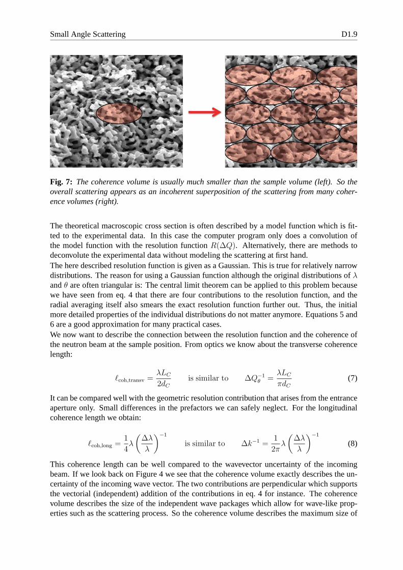
Fig. 7: The coherence volume is usually much smaller than the samplevolume (left). So theoverall scattering appears as an incoherent superpositionof the scattering from many coher-ence volumes (right).
The theoretical macroscopic cross section is often described by a model function which is fit-ted to the experimental data. In this case the computer program only does a convolution ofthe model function with the resolution functionR(∆Q). Alternatively, there are methods todeconvolute the experimental data without modeling the scattering at first hand.The here described resolution function is given as a Gaussian. This is true for relatively narrowdistributions. The reason for using a Gaussian function although the original distributions ofλandθ are often triangular is: The central limit theorem can be applied to this problem becausewe have seen from eq. 4 that there are four contributions to the resolution function, and theradial averaging itself also smears the exact resolution function further out. Thus, the initialmore detailed properties of the individual distributions do not matter anymore. Equations 5 and6 are a good approximation for many practical cases.We now want to describe the connection between the resolution function and the coherence ofthe neutron beam at the sample position. From optics we know about the transverse coherencelength:
ℓcoh,transv =λLC
2dCis similar to ∆Q−1
θ =λLC
πdC(7)
It can be compared well with the geometric resolution contribution that arises from the entranceaperture only. Small differences in the prefactors we can safely neglect. For the longitudinalcoherence length we obtain:
ℓcoh,long =1
4λ
(
∆λ
λ
)−1
is similar to ∆k−1 =1
2πλ
(
∆λ
λ
)−1
(8)
This coherence length can be well compared to the wavevectoruncertainty of the incomingbeam. If we look back on Figure 4 we see that the coherence volume exactly describes the un-certainty of the incoming wave vector. The two contributions are perpendicular which supportsthe vectorial (independent) addition of the contributionsin eq. 4 for instance. The coherencevolume describes the size of the independent wave packages which allow for wave-like prop-erties such as the scattering process. So the coherence volume describes the maximum size of
D1.10 H. Frielinghaus
structure that is observable by SANS. If larger structures need to be detected the resolution mustbe increased.The understanding how the small coherence volume covers thewhole sample volume is given inthe following (see also Fig. 7). Usually the coherence volume is rather small and is many timessmaller than the irradiated sample volume. So many independent coherence volumes cover thewhole sample. Then, the overall scattering intensity occurs as an independent sum from thescattering intensities of all coherence volumes. This is called incoherent superposition.
2.5 The theory of the macroscopic cross section (the Born approximation)
We have seen that the SANS instrument aims at the macroscopiccross section which is a func-tion of the scattering vectorQ. In many examples of isotropic samples and orientationallyaveraged samples (powder samples) the macroscopic cross section depends on the modulus|Q| ≡ Q only. This measured function has to be connected to important structural parametersof the sample. For this purpose model functions are developed. The shape of the model func-tion in comparison with the measurement already allows to distinguish the validity of the model.After extracting a few parameters with this method, deeper theories – like thermodynamics –allow to get deeper insight about the behavior of the sample.Usually, other parameters – likeconcentration, temperature, electric and magnetic fields,... – are varied experimentally to verifythe underlying concepts at hand. The purpose of this and the following sections is to give someideas about model functions.We have obtained a clear picture of the Born approximation in section 2.2. More formally, theBorn approximation arises from quantum mechanics, and several facts and assumptions camealong: The scattering amplitudes of the outgoing waves are derived as perturbations of the in-coming plane wave. The matrix elements of the interaction potential with these two wave fieldsas vectors describe the desired amplitudes. The interaction potential can be simplified for neu-trons and the nuclei of the sample by the Fermi pseudo potential. This expresses the smallnessof the nuclei (∼1fm) in comparison to the neutron wavelength (∼A). For the macroscopic crosssection we immediately obtain a sum over all nuclei:
dΣ
dΩ(Q) =
1
V
∣
∣
∣
∣
∣
∑
j
bj exp(iQ · rj)∣
∣
∣
∣
∣
2
(9)
This expression is normalized to the sample volumeV because the second factor usually is pro-portional to the sample size. This simply means: The more sample we put in the beam the moreintensity we obtain. The second factor is the square of the amplitude because we measure inten-sities. While for electromagnetic fields at low frequencies one can distinguish amplitudes andphases (without relying on the intensity) the neutrons are quantum mechanical particles whereexperimentally such details are hardly accessible. For light (and neutrons) for instance holo-graphic methods still remain. The single amplitude is a sum over each nucleusj with its typicalscattering lengthbj and a phase described by the exponential. The square of the scatteringlengthb2j describes a probability of a scattering event taking place for an isolated nucleus. Thephase arises between different elementary scattering events of the nuclei for the large distancesof the detector. In principle, the scattering length can be negative (for hydrogen for instance)which indicates an attractive interaction with a phaseπ. Complex scattering lengths indicateabsorption. The quadrature of the amplitude can be reorganized:
Small Angle Scattering D1.11
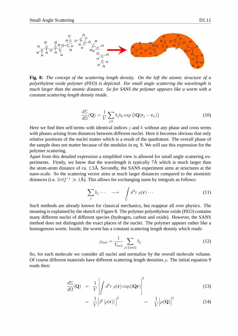
Fig. 8: The concept of the scattering length density. On the left theatomic structure of apolyethylene oxide polymer (PEO) is depicted. For small angle scattering the wavelength ismuch larger than the atomic distance. So for SANS the polymer appears like a worm with aconstant scattering length density inside.
dΣ
dΩ(Q) =
1
V
∑
j,k
bjbk exp(
iQ(rj − rk))
(10)
Here we find then self-terms with identical indicesj andk without any phase and cross termswith phases arising from distances between different nuclei. Here it becomes obvious that onlyrelative positions of the nuclei matter which is a result of the quadrature. The overall phase ofthe sample does not matter because of the modulus in eq. 9. We will use this expression for thepolymer scattering.Apart from this detailed expression a simplified view is allowed for small angle scattering ex-periments. Firstly, we know that the wavelength is typically 7A which is much larger thanthe atom-atom distance of ca. 1.5A. Secondly, the SANS experiment aims at structures at thenano-scale. So the scattering vector aims at much larger distances compared to the atomisticdistances (i.e.2πQ−1 ≫ 1A). This allows for exchanging sums by integrals as follows:
∑
j
bj · · · −→∫
V
d3r ρ(r) · · · (11)
Such methods are already known for classical mechanics, butreappear all over physics. Themeaning is explained by the sketch of Figure 8. The polymer polyethylene oxide (PEO) containsmany different nuclei of different species (hydrogen, carbon and oxide). However, the SANSmethod does not distinguish the exact places of the nuclei. The polymer appears rather like ahomogenous worm. Inside, the worm has a constant scatteringlength density which reads:
ρmol =1
Vmol
∑
j∈mol
bj (12)
So, for each molecule we consider all nuclei and normalize bythe overall molecule volume.Of course different materials have different scattering length densitiesρ. The initial equation 9reads then:
dΣ
dΩ(Q) =
1
V
∣
∣
∣
∣
∣
∣
∫
V
d3r ρ(r) exp(iQr)
∣
∣
∣
∣
∣
∣
2
(13)
=1
V
∣
∣
∣F [ρ(r)]
∣
∣
∣
2
=1
V
∣
∣
∣ρ(Q)
∣
∣
∣
2
(14)
D1.12 H. Frielinghaus
The single amplitude is now interpreted as a Fourier transformation of the scattering lengthdensityρ(r) which we simply indicate byρ(Q). The amplitude is defined by:
ρ(Q) =
∫
V
d3r ρ(r) exp(iQr) (15)
Again, equation 13 loses the phase information due to the modulus.
2.6 Spherical colloidal particles
In this section we will derive the scattering of diluted spherical particles in a solvent. Theseparticles are often called colloids, and can be of inorganicmaterial while the solvent is eitherwater or organic solvent. Later in the manuscript interactions will be taken into account.One important property of Fourier transformations is that constant contributions will lead tosharp delta peaks atQ = 0. This contribution is not observable in the practical scatteringexperiment. The theoretically sharp delta peak might have afinite width which is connectedto the overall sample size, but centimeter dimensions are much higher compared to the largestsizes observed by the scattering experiment (∼µm). So formally we can elevate the scatteringdensity level by any number−ρref :
The resulting delta peaks can simply be neglected. For a spherical particle we then arrive at thesimple scattering length density profile:
ρsingle(r) =
∆ρ for |r| ≤ R
0 for |r| > R(17)
Inside the sphere the value is constant because we assume homogenous particles. The referencescattering length density is given by the solvent. This function will then be Fourier transformedaccordingly:
ρsingle(Q) =
2π∫
0
dφ
π∫
0
dϑ sinϑ
R∫
0
dr r2 ∆ρ exp(
i|Q| · |r| cos(ϑ))
(18)
= 2π ∆ρ
R∫
0
dr r2[
1
iQrexp
(
iQrX)
]X=+1
X=−1
(19)
= 4π ∆ρ
R∫
0
dr r2sin(Qr)
Qr(20)
= ∆ρ4π
3R3
(
3sin(QR)−QR cos(QR)
(QR)3
)
(21)
In the first line 18 we introduce spherical coordinates with the vectorQ determining thez-axis for the real space. The vector productQr then leads to the cosine term. In line 19 the
Small Angle Scattering D1.13
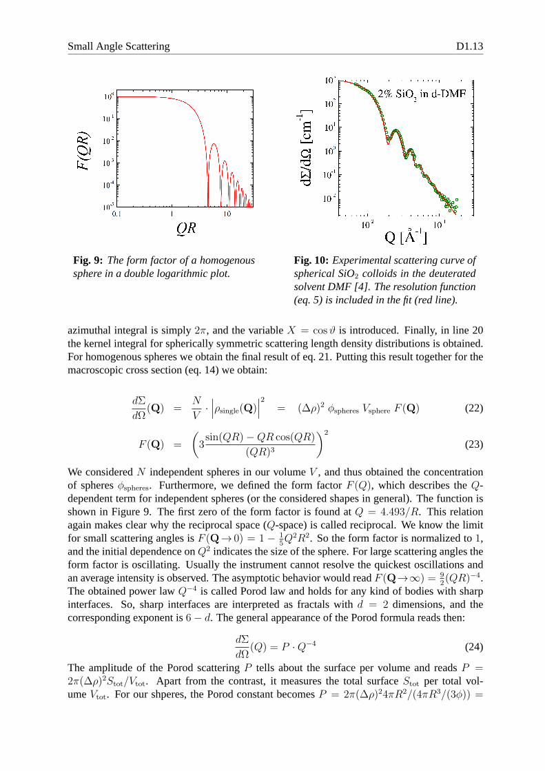
Fig. 9: The form factor of a homogenoussphere in a double logarithmic plot.
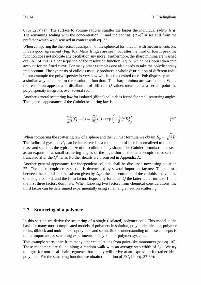
Fig. 10: Experimental scattering curve ofspherical SiO2 colloids in the deuteratedsolvent DMF [4]. The resolution function(eq. 5) is included in the fit (red line).
azimuthal integral is simply2π, and the variableX = cosϑ is introduced. Finally, in line 20the kernel integral for spherically symmetric scattering length density distributions is obtained.For homogenous spheres we obtain the final result of eq. 21. Putting this result together for themacroscopic cross section (eq. 14) we obtain:
dΣ
dΩ(Q) =
N
V·∣
∣
∣ρsingle(Q)
∣
∣
∣
2
= (∆ρ)2 φspheres Vsphere F (Q) (22)
F (Q) =
(
3sin(QR)−QR cos(QR)
(QR)3
)2
(23)
We consideredN independent spheres in our volumeV , and thus obtained the concentrationof spheresφspheres. Furthermore, we defined the form factorF (Q), which describes theQ-dependent term for independent spheres (or the considered shapes in general). The function isshown in Figure 9. The first zero of the form factor is found atQ = 4.493/R. This relationagain makes clear why the reciprocal space (Q-space) is called reciprocal. We know the limitfor small scattering angles isF (Q→ 0) = 1 − 1
5Q2R2. So the form factor is normalized to1,
and the initial dependence onQ2 indicates the size of the sphere. For large scattering angles theform factor is oscillating. Usually the instrument cannot resolve the quickest oscillations andan average intensity is observed. The asymptotic behavior would readF (Q→∞) = 9
2(QR)−4.
The obtained power lawQ−4 is called Porod law and holds for any kind of bodies with sharpinterfaces. So, sharp interfaces are interpreted as fractals with d = 2 dimensions, and thecorresponding exponent is6− d. The general appearance of the Porod formula reads then:
dΣ
dΩ(Q) = P ·Q−4 (24)
The amplitude of the Porod scatteringP tells about the surface per volume and readsP =2π(∆ρ)2Stot/Vtot. Apart from the contrast, it measures the total surfaceStot per total vol-umeVtot. For our shperes, the Porod constant becomesP = 2π(∆ρ)24πR2/(4πR3/(3φ)) =
D1.14 H. Frielinghaus
6πφ1(∆ρ)2/R. The surface to volume ratio is smaller the larger the individual radiusR is.The remaining scaling with the concentrationφ1 and the contrast(∆ρ)2 arises still from theprefactor which we discussed in context with eq. 22.
When comparing the theoretical description of the sphericalform factor with measurements onefinds a good agreement (Fig. 10). Many fringes are seen, but after the third or fourth peak thefunction does not indicate any oscillation any more. Furthermore, the sharp minima are washedout. All of this is a consequence of the resolution function (eq. 5) which has been taken intoaccount for the fitted curve. For many other examples one alsoneeds to take the polydispersityinto account. The synthesis of colloids usually produces a whole distribution of different radii.In our example the polydispersity is very low which is the desired case. Polydispersity acts ina similar way compared to the resolution function. The sharpminima are washed out. Whilethe resolution appears as a distribution of differentQ-values measured at a certain point thepolydispersity integrates over several radii.
Another general scattering law for isolated (dilute) colloids is found for small scattering angles.The general appearance of the Guinier scattering law is:
dΣ
dΩ(Q→0) =
dΣ
dΩ(0) · exp
(
−1
3Q2R2
g
)
(25)
When comparing the scattering law of a sphere and the Guinier formula we obtainRg =√
35R.
The radius of gyrationRg can be interpreted as a momentum of inertia normalized to thetotalmass and specifies the typical size of the colloid of any shape. The Guinier formula can be seenas an expansion at small scattering angles of the logarithm of the macroscopic cross sectiontruncated after theQ2 term. Further details are discussed in Appendix A.
Another general appearance for independent colloids shallbe discussed now using equation22. The macroscopic cross section is determined by several important factors: The contrastbetween the colloid and the solvent given by∆ρ2, the concentration of the colloids, the volumeof a single colloid, and the form factor. Especially for small Q the latter factor turns to1, andthe first three factors dominate. When knowing two factors from chemical considerations, thethird factor can be determined experimentally using small angle neutron scattering.
2.7 Scattering of a polymer
In this section we derive the scattering of a single (isolated) polymer coil. This model is thebasis for many more complicated models of polymers in solution, polymeric micelles, polymermelts, diblock and multiblock copolymers and so on. So the understanding of these concepts israther important for scattering experiments on any kind of polymer systems.
This example starts apart from many other calculations frompoint-like monomers (see eq. 10).These monomers are found along a random walk with an average step width ofℓK . We tryto argue for non-ideal chain segments, but finally will arrive at an expression for rather idealpolymers. For the scattering function we obtain (definitionof S(Q) in eq. 37-39):
Small Angle Scattering D1.15
S(Q) ∝ 1
N
N∑
j,k=0
⟨
exp (iQ · (Rj −Rk))⟩
(26)
∝ 1
N
N∑
j,k=0
exp⟨
−12(Q · (Rj −Rk))
2⟩
(27)
∝ 1
N
N∑
j,k=0
exp⟨
−16Q2 · (Rj −Rk)
2⟩
(28)
At this stage we use statistical arguments (i.e. statistical physics). The first rearrangement ofterms (line 27) moves the ensemble average of the monomer positions (and distances∆Rjk)from the outside of the exponential to the inside. This is an elementary step which is truefor polymers. The underlying idea is, that the distance∆Rjk arises from a sum of|j − k|bond vectors which all have the same statistics. So each sub-chain with the indicesjk is onlydistinguished by its number of bond vectors inside. The single bond vectorbj has a statisticalaverage of〈bj〉 = 0 because there is no preferred orientation. The next higher moment is thesecond moment〈b2
j〉 = ℓ2K . This describes that each bond vector does a finite step with anaverage length ofℓK . For the sub-chain we then find an average size〈∆R2
jk〉 = |j − k|ℓ2K . Thereason is that in the quadrature of the sub-chain only the diagonal terms contribute because twodistinct bond vectors show no (or weak) correlations.Back to the ensemble average: The original exponential can beseen as a Taylor expansionwith all powers of the argumentiQ∆Rjk. The odd powers do not contribute with similararguments than for the single bond vector〈bj〉 = 0. Thus, the quadratic term is the leading term.The reason why the higher order terms can be arranged that they finally fit to the exponentialexpression given in line 27 is the weak correlations of two distinct bond vectors. The next line28 basically expresses the orientational average of the sub-chain vector∆Rjk with respect totheQ-vector in three dimensions.This derivation can be even simpler understood on the basis of a Gaussian chain. Then everybond vector follows a Gaussian distribution (with a center of zero bond length). Then theensemble average has the concrete meaning〈· · · 〉 =
∫
· · · exp(
− 32∆R2
jk/(|j−k|ℓ2K))
d3∆Rjk.This distribution immediately explains the rearrangementof line 27. The principal argument isthe central limit theorem: When embracing several segments as an effective segment any kind ofdistribution converges to yield a Gaussian distribution. This idea came from Kuhn who formedthe term Kuhn segment. While elementary bonds still may have correlations at the stage of theKuhn segment all correlations are lost, and the chain reallybehaves ideal. This is the reasonwhy the Kuhn segment lengthℓK was already used in the above equations.In the following we now use the average length of sub-chains (be it Kuhn segments or not),and replace the sums by integrals which is a good approximation for long chains with a largenumber of segmentsN .
S(Q) ∝ 1
N
N∫
0
dj
N∫
0
dk exp(
−16Q2 · |j − k| · ℓ2K
)
(29)
= N · fD(Q2R2g) (30)
D1.16 H. Frielinghaus
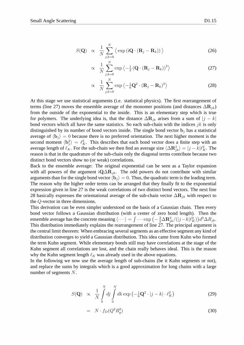
Fig. 11: The theoretical Debye functiondescribes the polymer scattering of in-dependent polymers without interaction.The two plots show the function on a lin-ear and double logarithmic scale.
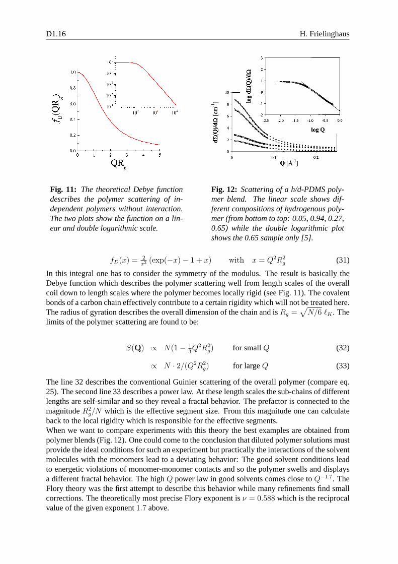
Fig. 12: Scattering of a h/d-PDMS poly-mer blend. The linear scale shows dif-ferent compositions of hydrogenous poly-mer (from bottom to top: 0.05, 0.94, 0.27,0.65) while the double logarithmic plotshows the 0.65 sample only [5].
fD(x) =2x2 (exp(−x)− 1 + x) with x = Q2R2
g (31)
In this integral one has to consider the symmetry of the modulus. The result is basically theDebye function which describes the polymer scattering wellfrom length scales of the overallcoil down to length scales where the polymer becomes locallyrigid (see Fig. 11). The covalentbonds of a carbon chain effectively contribute to a certain rigidity which will not be treated here.The radius of gyration describes the overall dimension of the chain and isRg =
√
N/6 ℓK . Thelimits of the polymer scattering are found to be:
S(Q) ∝ N(1− 13Q2R2
g) for smallQ (32)
∝ N · 2/(Q2R2g) for largeQ (33)
The line 32 describes the conventional Guinier scattering of the overall polymer (compare eq.25). The second line 33 describes a power law. At these lengthscales the sub-chains of differentlengths are self-similar and so they reveal a fractal behavior. The prefactor is connected to themagnitudeR2
g/N which is the effective segment size. From this magnitude onecan calculateback to the local rigidity which is responsible for the effective segments.When we want to compare experiments with this theory the best examples are obtained frompolymer blends (Fig. 12). One could come to the conclusion that diluted polymer solutions mustprovide the ideal conditions for such an experiment but practically the interactions of the solventmolecules with the monomers lead to a deviating behavior: The good solvent conditions leadto energetic violations of monomer-monomer contacts and sothe polymer swells and displaysa different fractal behavior. The highQ power law in good solvents comes close toQ−1.7. TheFlory theory was the first attempt to describe this behavior while many refinements find smallcorrections. The theoretically most precise Flory exponent is ν = 0.588 which is the reciprocalvalue of the given exponent1.7 above.
Small Angle Scattering D1.17
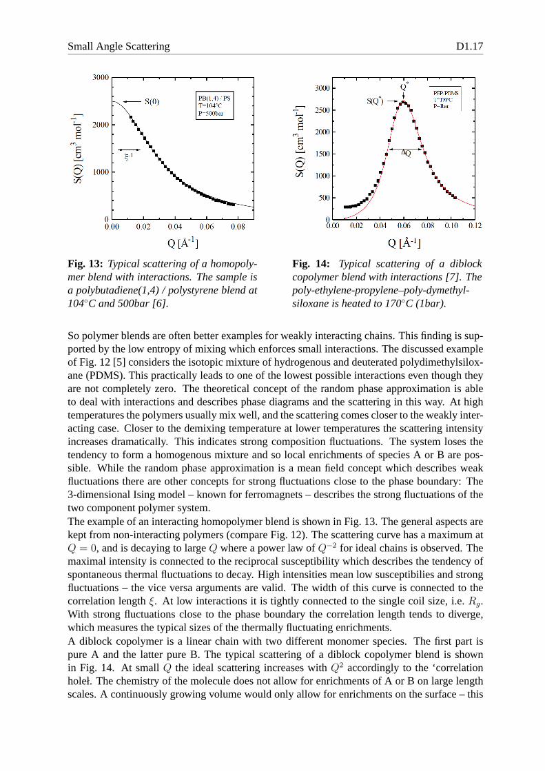
Fig. 13: Typical scattering of a homopoly-mer blend with interactions. The sample isa polybutadiene(1,4) / polystyrene blend at104C and 500bar [6].
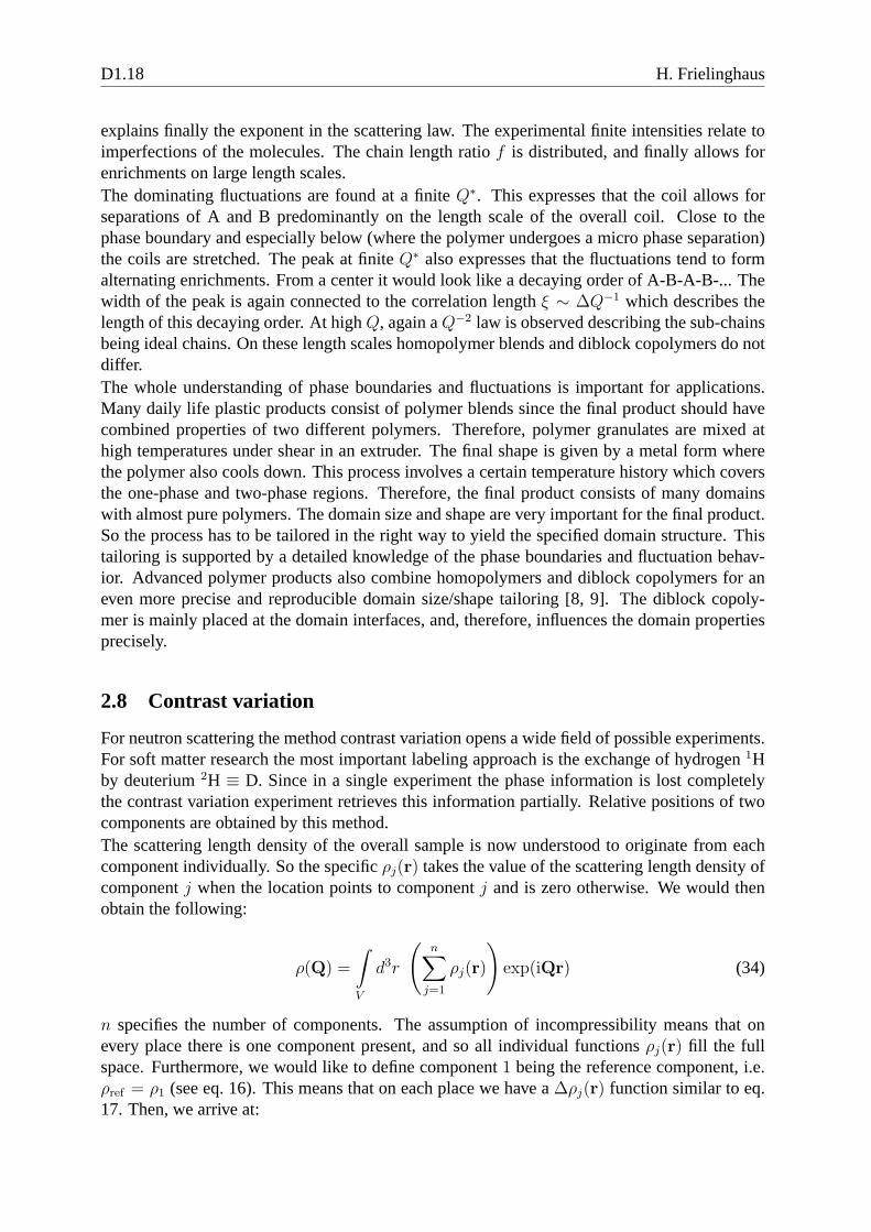
Fig. 14: Typical scattering of a diblockcopolymer blend with interactions [7]. Thepoly-ethylene-propylene–poly-dymethyl-siloxane is heated to 170C (1bar).
So polymer blends are often better examples for weakly interacting chains. This finding is sup-ported by the low entropy of mixing which enforces small interactions. The discussed exampleof Fig. 12 [5] considers the isotopic mixture of hydrogenousand deuterated polydimethylsilox-ane (PDMS). This practically leads to one of the lowest possible interactions even though theyare not completely zero. The theoretical concept of the random phase approximation is ableto deal with interactions and describes phase diagrams and the scattering in this way. At hightemperatures the polymers usually mix well, and the scattering comes closer to the weakly inter-acting case. Closer to the demixing temperature at lower temperatures the scattering intensityincreases dramatically. This indicates strong composition fluctuations. The system loses thetendency to form a homogenous mixture and so local enrichments of species A or B are pos-sible. While the random phase approximation is a mean field concept which describes weakfluctuations there are other concepts for strong fluctuations close to the phase boundary: The3-dimensional Ising model – known for ferromagnets – describes the strong fluctuations of thetwo component polymer system.The example of an interacting homopolymer blend is shown in Fig. 13. The general aspects arekept from non-interacting polymers (compare Fig. 12). The scattering curve has a maximum atQ = 0, and is decaying to largeQ where a power law ofQ−2 for ideal chains is observed. Themaximal intensity is connected to the reciprocal susceptibility which describes the tendency ofspontaneous thermal fluctuations to decay. High intensities mean low susceptibilies and strongfluctuations – the vice versa arguments are valid. The width of this curve is connected to thecorrelation lengthξ. At low interactions it is tightly connected to the single coil size, i.e.Rg.With strong fluctuations close to the phase boundary the correlation length tends to diverge,which measures the typical sizes of the thermally fluctuating enrichments.A diblock copolymer is a linear chain with two different monomer species. The first part ispure A and the latter pure B. The typical scattering of a diblock copolymer blend is shownin Fig. 14. At smallQ the ideal scattering increases withQ2 accordingly to the ‘correlationholeł. The chemistry of the molecule does not allow for enrichments of A or B on large lengthscales. A continuously growing volume would only allow for enrichments on the surface – this
D1.18 H. Frielinghaus
explains finally the exponent in the scattering law. The experimental finite intensities relate toimperfections of the molecules. The chain length ratiof is distributed, and finally allows forenrichments on large length scales.The dominating fluctuations are found at a finiteQ∗. This expresses that the coil allows forseparations of A and B predominantly on the length scale of the overall coil. Close to thephase boundary and especially below (where the polymer undergoes a micro phase separation)the coils are stretched. The peak at finiteQ∗ also expresses that the fluctuations tend to formalternating enrichments. From a center it would look like a decaying order of A-B-A-B-... Thewidth of the peak is again connected to the correlation length ξ ∼ ∆Q−1 which describes thelength of this decaying order. At highQ, again aQ−2 law is observed describing the sub-chainsbeing ideal chains. On these length scales homopolymer blends and diblock copolymers do notdiffer.The whole understanding of phase boundaries and fluctuations is important for applications.Many daily life plastic products consist of polymer blends since the final product should havecombined properties of two different polymers. Therefore,polymer granulates are mixed athigh temperatures under shear in an extruder. The final shapeis given by a metal form wherethe polymer also cools down. This process involves a certaintemperature history which coversthe one-phase and two-phase regions. Therefore, the final product consists of many domainswith almost pure polymers. The domain size and shape are veryimportant for the final product.So the process has to be tailored in the right way to yield the specified domain structure. Thistailoring is supported by a detailed knowledge of the phase boundaries and fluctuation behav-ior. Advanced polymer products also combine homopolymers and diblock copolymers for aneven more precise and reproducible domain size/shape tailoring [8, 9]. The diblock copoly-mer is mainly placed at the domain interfaces, and, therefore, influences the domain propertiesprecisely.
2.8 Contrast variation
For neutron scattering the method contrast variation opensa wide field of possible experiments.For soft matter research the most important labeling approach is the exchange of hydrogen1Hby deuterium2H ≡ D. Since in a single experiment the phase information is lostcompletelythe contrast variation experiment retrieves this information partially. Relative positions of twocomponents are obtained by this method.The scattering length density of the overall sample is now understood to originate from eachcomponent individually. So the specificρj(r) takes the value of the scattering length density ofcomponentj when the location points to componentj and is zero otherwise. We would thenobtain the following:
ρ(Q) =
∫
V
d3r
(
n∑
j=1
ρj(r)
)
exp(iQr) (34)
n specifies the number of components. The assumption of incompressibility means that onevery place there is one component present, and so all individual functionsρj(r) fill the fullspace. Furthermore, we would like to define component1 being the reference component, i.e.ρref = ρ1 (see eq. 16). This means that on each place we have a∆ρj(r) function similar to eq.17. Then, we arrive at:
Small Angle Scattering D1.19
ρ(Q) =n∑
j=2
∆ρj1(Q) (35)
The macroscopic cross section is a quadrature of the scattering length densityρ(Q), and so wearrive at:
dΣ
dΩ(Q) =
1
V·
n∑
j,k=2
∆ρ∗j1(Q) ·∆ρk1(Q) (36)
=n∑
j,k=2
(∆ρj1∆ρk1) · Sjk(Q) (37)
=n∑
j=2
(∆ρj1)2 · Sjj(Q) + 2
∑
2<j<k≤n
(∆ρj1∆ρk1) · ℜ Sjk(Q) (38)
In line 37 the scattering functionSjk(Q) is defined. By this the contrasts are separated from theQ-dependent scattering functions. Finally, in line 38 the diagonal and off-diagonal terms arecollected. There aren − 1 diagonal terms, and1
2(n − 1)(n − 2) off-diagonal terms. Formally,
these12n(n − 1) considerably different terms are rearranged (the combinationsj, k are now
simply numbered byj), and a number ofs different measurements with different contrasts areconsidered.
dΣ
dΩ(Q)
∣
∣
∣
∣
s
=∑
j
(∆ρ ·∆ρ)sj · Sj(Q) (39)
In order to reduce the noise of the result, the number of measurementss exceeds the numberof independent scattering functions considerably. The system then becomes over-determinedwhen solving for the scattering functions. Formally, one can nonetheless write:
Sj(Q) =∑
s
(∆ρ ·∆ρ)−1sj · dΣ
dΩ(Q)
∣
∣
∣
∣
s
(40)
The formal inverse matrix(∆ρ ·∆ρ)−1sj is obtained by the singular value decomposition method.
It describes the closest solution of the experiments in context of the finally determined scatteringfunctions.An example case is discussed for a bicontinuous microemulsion with an amphiphilic polymer[10]. The microemulsion consists of oil and water domains which have a sponge structure. Sothe water domains host the oil and vice versa. The surfactantfilm covers the surface between theoil and water domains. The symmetric amphiphilic polymer position and function was not clearbeforehand. From phase diagram measurements it was observed that the polymer increases theefficiency of the surfactant dramatically. Much less surfactant is needed to solubilize equalamounts of oil and water. Fig. 15 discusses the meaning of thecross terms of the scatteringfunctions. Especially the film-polymer scattering is highly interesting to reveal the polymerrole inside the microemulsion (see Fig. 16). By the modeling it was clearly observed that theamphiphilic polymer is anchored in the membrane and the two blocks describe a mushroominside the oil and water domains. So basically, the polymer is a macro-surfactant. The coils ofthe polymer exert a certain pressure on the membrane and keepit flat. The membrane with less
D1.20 H. Frielinghaus
Fig. 15: Scheme of scattering functionsfor the cross terms within the microemul-sion. There are the film-polymer scatter-ing SFP, the oil-film scatteringSOF, andthe oil-polymer scatteringSOP. The realspace correlation function means a con-volution of two structures.
Fig. 16: A measurement of the film-polymer scattering for a bicontinuousmicroemulsion with a symmetric am-phiphilic polymer. The solid line is de-scribed by a polymer anchored in thefilm. The two blocks are mushroom-likein the domains. At lowQ the overall do-main structure (or size) limits the ideal-ized model picture.
fluctuations allows for the formation of larger domains witha better surface to volume ratio.This is finally the explanation how the polymer acts as an efficiency booster.
3 Small Angle X-ray Scattering
While a detailed comparison between SANS and SAXS is given below, the most importantproperties of the small angle x-ray scattering technique shall be discussed here. The x-raysources can be x-ray tubes (invented by Rontgen, keyword Bremsstrahlung) and modern syn-chrotrons. The latter ones guide fast electrons on undulators which act as laser-like sources forx-rays with fixed wavelength, high brilliance and low divergence. This simply means, that thecollimation of the beam often yields narrow beams, and the irradiated sample areas are consid-erably smaller (often smaller than ca. 1×1mm2). A view on the sample position is given in Fig.17 (compare Fig. 3). One directly has the impression that allwindows are tiny and adjustmentsmust be made more carefully.
The conceptual understanding of the scattering theory still holds for SAXS. For the simplestunderstanding of the contrast conditions in a SAXS experiment, it is sufficient to count theelectron numbers for each atom. The resulting scattering length density reads then (compareeq. 12):
Small Angle Scattering D1.21
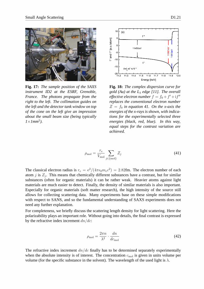
Fig. 17: The sample position of the SAXSinstrument ID2 at the ESRF, Grenoble,France. The photons propagate from theright to the left. The collimation guides onthe left and the detector tank window on topof the cone on the left give an impressionabout the small beam size (being typically1×1mm2).
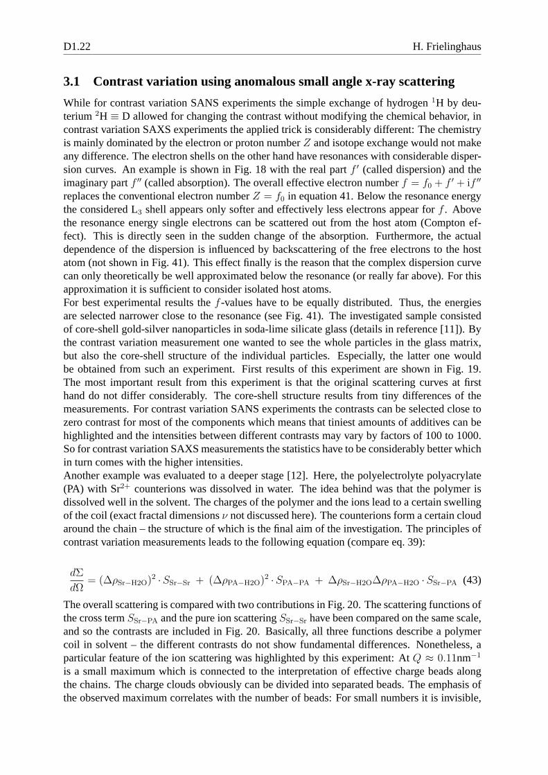
Fig. 18: The complex dispersion curve forgold (Au) at the L3 edge [11]. The overalleffective electron numberf = f0+ f ′+if ′′
replaces the conventional electron numberZ = f0 in equation 41. On the x-axis theenergies of the x-rays is shown, with indica-tions for the experimentally selected threeenergies (black, red, blue). In this way,equal steps for the contrast variation areachieved.
ρmol =reVmol
∑
j∈mol
Zj (41)
The classical electron radius isre = e2/(4πǫ0mec2) = 2.82fm. The electron number of each
atomj is Zj. This means that chemically different substances have a contrast, but for similarsubstances (often for organic materials) it can be rather weak. Heavier atoms against lightmaterials are much easier to detect. Finally, the density ofsimilar materials is also important.Especially for organic materials (soft matter research), the high intensity of the source stillallows for collecting scattering data. Many experiments base on these simple modificationswith respect to SANS, and so the fundamental understanding of SAXS experiments does notneed any further explanation.
For completeness, we briefly discuss the scattering length density for light scattering. Here thepolarizability plays an important role. Without going intodetails, the final contrast is expressedby the refractive index incrementdn/dc:
ρmol =2πn
λ2· dn
dcmol
(42)
The refractive index incrementdn/dc finally has to be determined separately experimentallywhen the absolute intensity is of interest. The concentration cmol is given in units volume pervolume (for the specific substance in the solvent). The wavelength of the used light isλ.
D1.22 H. Frielinghaus
3.1 Contrast variation using anomalous small angle x-ray scattering
While for contrast variation SANS experiments the simple exchange of hydrogen1H by deu-terium 2H ≡ D allowed for changing the contrast without modifying the chemical behavior, incontrast variation SAXS experiments the applied trick is considerably different: The chemistryis mainly dominated by the electron or proton numberZ and isotope exchange would not makeany difference. The electron shells on the other hand have resonances with considerable disper-sion curves. An example is shown in Fig. 18 with the real partf ′ (called dispersion) and theimaginary partf ′′ (called absorption). The overall effective electron number f = f0 + f ′ + if ′′
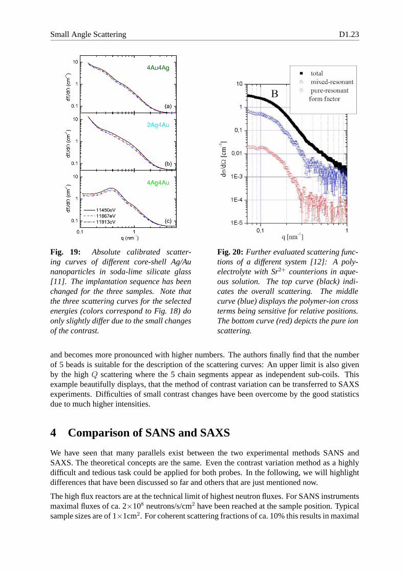
replaces the conventional electron numberZ = f0 in equation 41. Below the resonance energythe considered L3 shell appears only softer and effectively less electrons appear forf . Abovethe resonance energy single electrons can be scattered out from the host atom (Compton ef-fect). This is directly seen in the sudden change of the absorption. Furthermore, the actualdependence of the dispersion is influenced by backscattering of the free electrons to the hostatom (not shown in Fig. 41). This effect finally is the reason that the complex dispersion curvecan only theoretically be well approximated below the resonance (or really far above). For thisapproximation it is sufficient to consider isolated host atoms.For best experimental results thef -values have to be equally distributed. Thus, the energiesare selected narrower close to the resonance (see Fig. 41). The investigated sample consistedof core-shell gold-silver nanoparticles in soda-lime silicate glass (details in reference [11]). Bythe contrast variation measurement one wanted to see the whole particles in the glass matrix,but also the core-shell structure of the individual particles. Especially, the latter one wouldbe obtained from such an experiment. First results of this experiment are shown in Fig. 19.The most important result from this experiment is that the original scattering curves at firsthand do not differ considerably. The core-shell structure results from tiny differences of themeasurements. For contrast variation SANS experiments thecontrasts can be selected close tozero contrast for most of the components which means that tiniest amounts of additives can behighlighted and the intensities between different contrasts may vary by factors of 100 to 1000.So for contrast variation SAXS measurements the statisticshave to be considerably better whichin turn comes with the higher intensities.Another example was evaluated to a deeper stage [12]. Here, the polyelectrolyte polyacrylate(PA) with Sr2+ counterions was dissolved in water. The idea behind was thatthe polymer isdissolved well in the solvent. The charges of the polymer andthe ions lead to a certain swellingof the coil (exact fractal dimensionsν not discussed here). The counterions form a certain cloudaround the chain – the structure of which is the final aim of theinvestigation. The principles ofcontrast variation measurements leads to the following equation (compare eq. 39):
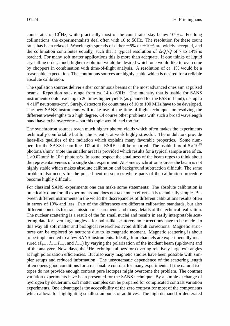
The overall scattering is compared with two contributions in Fig. 20. The scattering functions ofthe cross termSSr−PA and the pure ion scatteringSSr−Sr have been compared on the same scale,and so the contrasts are included in Fig. 20. Basically, all three functions describe a polymercoil in solvent – the different contrasts do not show fundamental differences. Nonetheless, aparticular feature of the ion scattering was highlighted bythis experiment: AtQ ≈ 0.11nm−1
is a small maximum which is connected to the interpretation of effective charge beads alongthe chains. The charge clouds obviously can be divided into separated beads. The emphasis ofthe observed maximum correlates with the number of beads: For small numbers it is invisible,
Small Angle Scattering D1.23
Fig. 19: Absolute calibrated scatter-ing curves of different core-shell Ag/Aunanoparticles in soda-lime silicate glass[11]. The implantation sequence has beenchanged for the three samples. Note thatthe three scattering curves for the selectedenergies (colors correspond to Fig. 18) doonly slightly differ due to the small changesof the contrast.
Fig. 20: Further evaluated scattering func-tions of a different system [12]: A poly-electrolyte with Sr2+ counterions in aque-ous solution. The top curve (black) indi-cates the overall scattering. The middlecurve (blue) displays the polymer-ion crossterms being sensitive for relative positions.The bottom curve (red) depicts the pure ionscattering.
and becomes more pronounced with higher numbers. The authors finally find that the numberof 5 beads is suitable for the description of the scattering curves: An upper limit is also givenby the highQ scattering where the 5 chain segments appear as independentsub-coils. Thisexample beautifully displays, that the method of contrast variation can be transferred to SAXSexperiments. Difficulties of small contrast changes have been overcome by the good statisticsdue to much higher intensities.
4 Comparison of SANS and SAXS
We have seen that many parallels exist between the two experimental methods SANS andSAXS. The theoretical concepts are the same. Even the contrast variation method as a highlydifficult and tedious task could be applied for both probes. In the following, we will highlightdifferences that have been discussed so far and others that are just mentioned now.
The high flux reactors are at the technical limit of highest neutron fluxes. For SANS instrumentsmaximal fluxes of ca. 2×10⁸ neutrons/s/cm2 have been reached at the sample position. Typicalsample sizes are of 1×1cm2. For coherent scattering fractions of ca. 10% this results in maximal
D1.24 H. Frielinghaus
count rates of 107Hz, while practically most of the count rates stay below 106Hz. For longcollimations, the experimentalists deal often with 10 to 50Hz. The resolution for these countrates has been relaxed. Wavelength spreads of either±5% or±10% are widely accepted, andthe collimation contributes equally, such that a typical resolution of∆Q/Q of 7 to 14% isreached. For many soft matter applications this is more thanadequate. If one thinks of liquidcrystalline order, much higher resolution would be desiredwhich one would like to overcomeby choppers in combination with time-of-flight analysis. A resolution of ca. 1% would be areasonable expectation. The continuous sources are highlystable which is desired for a reliableabsolute calibration.
The spallation sources deliver either continuous beams or the most advanced ones aim at pulsedbeams. Repetition rates range from ca. 14 to 60Hz. The intensity that is usable for SANSinstruments could reach up to 20 times higher yields (as planned for the ESS in Lund), i.e. up to4×109 neutrons/s/cm2. Surely, detectors for count rates of 10 to 100 MHz have to be developed.The new SANS instruments will make use of the time-of-flight technique for resolving thedifferent wavelengths to a high degree. Of course other problems with such a broad wavelengthband have to be overcome – but this topic would lead too far.
The synchrotron sources reach much higher photon yields which often makes the experimentstechnically comfortable but for the scientist at work highly stressful. The undulators providelaser-like qualities of the radiation which explains many favorable properties. Some num-bers for the SAXS beam line ID2 at the ESRF shall be reported. The usable flux of 5×10¹⁵
photons/s/mm2 (note the smaller area) is provided which results for a typical sample area of ca.1×0.02mm2 in 1014 photons/s. In some respect the smallness of the beam urges tothink aboutthe representativeness of a single shot experiment. At somesynchrotron sources the beam is nothighly stable which makes absolute calibration and background subtraction difficult. The sameproblem also occurs for the pulsed neutron sources where parts of the calibration procedurebecome highly difficult.
For classical SANS experiments one can make some statements: The absolute calibration ispractically done for all experiments and does not take much effort – it is technically simple. Be-tween different instruments in the world the discrepanciesof different calibrations results oftenin errors of 10% and less. Part of the differences are different calibration standards, but alsodifferent concepts for transmission measurements and manydetails of the technical realization.The nuclear scattering is a result of the fm small nuclei and results in easily interpretable scat-tering data for even large angles – for point-like scatterers no corrections have to be made. Inthis way all soft matter and biological researchers avoid difficult corrections. Magnetic struc-tures can be explored by neutrons due to its magnetic moment.Magnetic scattering is aboutto be implemented to a few SANS instruments. Ideally, four channels are experimentally mea-sured (I++, I+−,I−+, andI−−) by varying the polarization of the incident beam (up/down)andof the analyzer. Nowadays, the3He technique allows for covering relatively large exit anglesat high polarization efficiencies. But also early magnetic studies have been possible with sim-pler setups and reduced information. The unsystematic dependence of the scattering lengthoften opens good conditions for a reasonable contrast for many experiments. If the natural iso-topes do not provide enough contrast pure isotopes might overcome the problem. The contrastvariation experiments have been presented for the SANS technique. By a simple exchange ofhydrogen by deuterium, soft matter samples can be prepared for complicated contrast variationexperiments. One advantage is the accessibility of the zerocontrast for most of the componentswhich allows for highlighting smallest amounts of additives. The high demand for deuterated
Small Angle Scattering D1.25
chemicals makes them cheap caused by the huge number of NMR scientists. The low absorp-tion of neutrons for many materials allows for studying reasonably thick samples (1 to 5mmand beyond). Especially, for contrast variation experiments often larger optical path lengthsare preferred. The choice for window materials and sample containers is simple in many cases.Neutron scattering is a non-destructive method. Espeically biological samples can be recovered.
Contrarily we observe for the SAXS technique: The demand for absolute calibration in SAXSexperiments is growing. Initial technical problems are overcome and suitable calibration stan-dards have been found. The interpretation of scattering data at larger angles might be morecomplicated due to the structure of the electron shells. Forsmall angle scattering the possiblecorrections are often negligible. Magnetic structures areobservable by the circular magneticdichroism [13] but do not count to the standard problems addressed by SAXS. The high con-trast of heavy atoms often makes light atoms invisible. For soft matter samples the balanced useof light atoms results in low contrast but, technically, thebrilliant sources overcome any inten-sity problem. The ASAXS technique is done close to resonances of single electron shells andopens the opportunity for contrast variation measurements. The achieved small differences inthe contrast still allow for tedious measurements because the statistics are often extremely good– only stable experimental conditions have to be provided. The absorption of x-rays makes thechoice of sample containers and windows more complicated. The absorbed radiation destroysthe sample in principle. Short experimental times are thus favorable.
To summarize, the method of small angle neutron scattering is good-natured and allows totackle many difficult tasks. The small angle x-ray scattering technique is more often applieddue to the availability. Many problems have been solved (or will be solved) and will turn tostandard techniques. So, in many cases the competition between the methods is kept high forthe future. Today, practically, the methods are complementary and support each other for thecomplete structural analysis.
D1.26 H. Frielinghaus
Appendices
A Guinier Scattering
The crucial calculation of the Guinier scattering is done bya Taylor expansion of the logarithmof the macroscopic cross section for small scattering vectorsQ. Due to symmetry considerationsthere are no linear terms, and the dominating term of theQ-dependence is calculated to be:
R2g = −1
2· ∂2
∂Q2ln(
ρ(Q)ρ(−Q))
∣
∣
∣
∣
Q=0
(44)
= −1
2· ∂
∂Q
2ℜ(
ρ(Q)∫
d3r ρ(r)(−ir) exp(−iQr))
ρ(Q)ρ(−Q)
∣
∣
∣
∣
∣
Q=0
(45)
= −ℜρ(Q)∫
d3r ρ(r)(−r2) exp(−iQr)
ρ(Q)ρ(−Q)
∣
∣
∣
∣
Q=0
−ℜ∫
d3r ρ(r)(ir) exp(iQr)∫
d3r ρ(r)(−ir) exp(−iQr)
ρ(Q)ρ(−Q)
∣
∣
∣
∣
Q=0
+ 0 (46)
= 〈r2〉 − 〈r〉2 (47)
=⟨
(
r− 〈r〉)2⟩
(48)
The first line 44 contains the definition of the Taylor coefficient. Then, the derivatives arecalculated consequently. Finally, we arrive at terms containing the first and second momenta.The last line 48 rearranges the momenta in the sense of a variance. So the radius of gyrationis the second moment of the scattering length density distribution with the center of ‘gravity’being at the origin. We used the momenta in the following sense:
〈r〉 =
∫
d3r rρ(r)
/
∫
d3r ρ(r) (49)
〈r2〉 =
∫
d3r r2ρ(r)
/
∫
d3r ρ(r) (50)
So far we assumed an isotropic scattering length density distribution. In general, for orientedanisotropic particles, the Guinier scattering law would read:
dΣ
dΩ(Q→0) =
dΣ
dΩ(0) · exp
(
−Q2x
⟨
(
x− 〈x〉)2⟩
−Q2y
⟨
(
y − 〈y〉)2⟩
−Q2z
⟨
(
z − 〈z〉)2⟩)
(51)Here, we assumed a diagonal tensor of second moment. This expression allows for differentwidths of scattering patterns for the different directions. In reciprocal space large dimensionsappear small and vice versa. Furthermore, we see thatRg is defined as the sum over all secondmomenta, and so in the isotropic case a factor1
3appears in the original formula 25.
Small Angle Scattering D1.27
References
[1] R.-J. Roe,Methods of X-ray and Neutron Scattering in Polymer Science(Oxford Univer-sity Press, New York, 2000).
[10] H. Endo, M. Mihailescu, M. Monkenbusch, J. Allgaier, G.Gompper, D. Richter, B.Jakobs, T. Sottmann, R. Strey, I. Grillo,J. Chem. Phys.115, 580 (2001).
[11] J. Haug, H. Kruth, M. Dubiel, H. Hofmeister, S. Haas, D. Tatchev, A. Hoell,Nanotech-nology20, 505705 (2009).
[12] G. Goerigk, K. Huber, R. Schweins,J. Chem. Phys.127, 154908 (2007) and G. Goerigk,R. Schweins, K. Huber, M. Ballauff,Europhys. Lett.66, 331 (2004).
[13] P. Fischer, R. Zeller, G. Schutz, G. Goerigk, H.G. Haubold,J. Phys. IV France7, C2-753(1997).