Small-Kernel Super-Resolution Methods for

Microscanning Imaging Systems

Jiazheng Shi,∗ Stephen E. Reichenbach,∗ and James D. Howe†

∗Computer Science and Engineering Department,

University of Nebraska – Lincoln

†Night Vision and Electronic Sensors Directorate, U.S. Army

This paper presents two computationally efficient methods for super-

resolution reconstruction and restoration for microscanning imaging systems.

Microscanning creates multiple low-resolution images with slightly varying

sample-scene phase shifts. The digital processing methods developed in this

paper combine the low-resolution images to produce an image with higher

pixel resolution (i.e., super-resolution) and higher fidelity. The methods

implement reconstruction to increase resolution and restoration to improve

fidelity in one-pass convolution with a small kernel. One method is a small-

kernel Wiener filter and the other method is a parametric cubic convolution

filter (designated 2D-5PCC-R). Both methods are based on an end-to-end,

continuous-discrete-continuous (CDC) microscanning imaging system model.

Because the filters are constrained to small spatial kernels they can be effi-

ciently applied by convolution and are amenable to adaptive processing and to

parallel processing. Experimental results with simulated imaging and with real

microscanned images indicate that the small-kernel methods efficiently and

effectively increase resolution and fidelity. c© 2005 Optical Society of America

OCIS codes: 100.6640, 100.3020, 100.2000

1. Introduction

Improvements in the resolution and fidelity of digital imaging systems have substantial value

for remote sensing, military surveillance, and other applications, especially those for which

a large field-of-view is desirable and the distance to objects of interest cannot be reduced.

Advances in optics and sensor technologies offer one path for increasing the spatial resolution

and fidelity of imaging systems, but such hardware improvements can be costly and/or

1

limited by physical constraints.1,2 Digital image processing offers an alternative path for

improving image quality.

Digital super-resolution reconstruction and restoration methods can substantially increase

resolution and fidelity of an imaging system. Reconstruction methods increase pixel reso-

lution beyond that of the physical imaging system by estimating values on a finer grid or

lattice. Restoration methods increase fidelity beyond that of the physical imaging system

by correcting for acquisition artifacts such as blurring, aliasing, and noise. Super-resolution

reconstruction and restoration can be combined to produce images with greater resolution

and higher fidelity.3

Typically, super-resolution methods produce an enhanced image from multiple low-

resolution images with either different sample-scene phase or with different blurring func-

tions.4,5 Microscanning is a systematic approach for acquiring images with slightly differing

sample-scene phase — between successive images, the system is shifted slightly, either in a

predetermined pattern or in a random pattern. As in most super-resolution methods, the

methods developed in this paper presume global sample-scene phase shifts.

Most super-resolution methods can be decomposed into three tasks: registration, recon-

struction, and restoration. These tasks can be implemented as separate steps or in one or

two combined steps.

• Registration is the process of orienting several images of a common scene with ref-

erence to a single coordinate system. Registering images to subpixel accuracy is a

crucial factor that greatly impacts super-resolution processing. Systems with precisely

controlled phase-shifting may be trivial to register. Popular methods for subpixel im-

age registration include phase or cross correlation registration6,7 and gradient-based

registration.8,9

• Image reconstruction is the process of estimating the image value at arbitrary locations

on a spatial continuum from a set of discrete samples. For super-resolution imaging, the

aim of reconstruction is to produce an image with pixels on a high-resolution grid with

uniform spacing from the multiple, registered images which may have pixels that are

irregularly distributed. Popular methods for reconstruction include nearest neighbor

interpolation, bi-linear interpolation, cubic-spline interpolation, piecewise cubic convo-

lution, and cubic optimal maximal-order-minimal-support (o-Moms) interpolation.10

Kriging, which originated in the geostatistical community, is a popular method for

interpolating spatial data.11,12

• Image restoration is the process of recovering a more accurate image of a scene by

correcting or reducing degradations such as acquisition blurring, aliasing, and noise.13

Basic methods for image restoration include deconvolution, least-squares filters, and

2

iterative approaches.14

Digital processing for super-resolution is an area of active research.1,15 Approaches based

on non-uniform interpolation are the most intuitive. Computational efficiency is their major

advantage. For example, Alam et al. proposed a super-resolution method for infrared images,

using a gradient-based method to estimate shift, the weighted nearest-neighbor approach to

align irregularly displaced low-resolution images to form a super-resolution image, and finally

the Wiener filter for image restoration.9 However, nonuniform interpolation approaches do

not account for varying acquisition conditions for the low-resolution images nor guarantee the

optimality of the end-to-end imaging system.3 Tsai and Huang investigated super-resolution

imaging in frequency domain,16 using the shift theorem of the Fourier transform and the

aliasing relationship between low-resolution images and the ideal super-resolution image.

High frequency components are extracted from aliased low frequency components. Kim et

al. extended this approach for blurred and noisy images and developed a weighted recur-

sive least-squares algorithm.17,18 Unfortunately, Fourier-domain methods are computational

costly. Super-resolution methods based on stochastic theories employ a priori knowledge

about a scene and noise. For example, Shultz and Stevenson19 proposed a Bayesian restora-

tion with a discontinuity-preserving prior image model and Elad et al.5,20 approached super-

resolution by unifying the maximum likelihood (ML), maximum a posteriori (MAP), and

projection onto convex set (POCS). Stochastic approaches also may have high computational

complexity and sub-optimality for the end-to-end imaging system. Computationally efficient

spatial-domain methods have been proposed. Nguyen et al .21 proposed efficient block circu-

lant preconditioners for solving the Tikhonov regularized superresolution problems by using

the conjugate gradient method, but the method requires perfect shift estimation.22 Farsiu

et al . proposed a robust method that defines the cost function of regularization using the

L1 norm minimization.23 The method is robust for estimation errors of shift and noise, but

the system model accounts for only acquisition in the end-to-end system and the proposed

fast solution is iterative. Even though interpolation and restoration are done simultaneously,

computational costs for real-time applications are a concern with iterative methods.

This paper investigates super-resolution methods for microscanning imaging systems that

can be implemented efficiently with small convolution kernels. The approach is based on

an end-to-end, CDC system model that accounts for the fundamental tradeoff in imaging

system design between acquisition blurring related to optics, detectors, and analog circuits

and aliasing due to sampling. The system model also accounts for noise associated with

unpredictable signal and system variations and quantization, for mis-registration of the low-

resolution images, and for the display system. The approach uses one-pass convolution with

small kernels for computationally efficient reconstruction and restoration. This approach also

is amenable to adaptive processing and to parallel processing with appropriate hardware

3

support.

The rest of this paper is organized as follows. Section 2 presents the CDC system model, in-

troduces microscanning, and formulates the system fidelity. Section 3 derives super-resolution

reconstruction and restoration filters, including the optimal Wiener filter, a spatially con-

strained Wiener kernel, and a parametric cubic convolution kernel. Section 4 presents ex-

perimental results for images from a simulation and from a real imaging system. Section 5

summarizes this paper and describes issues for future work.

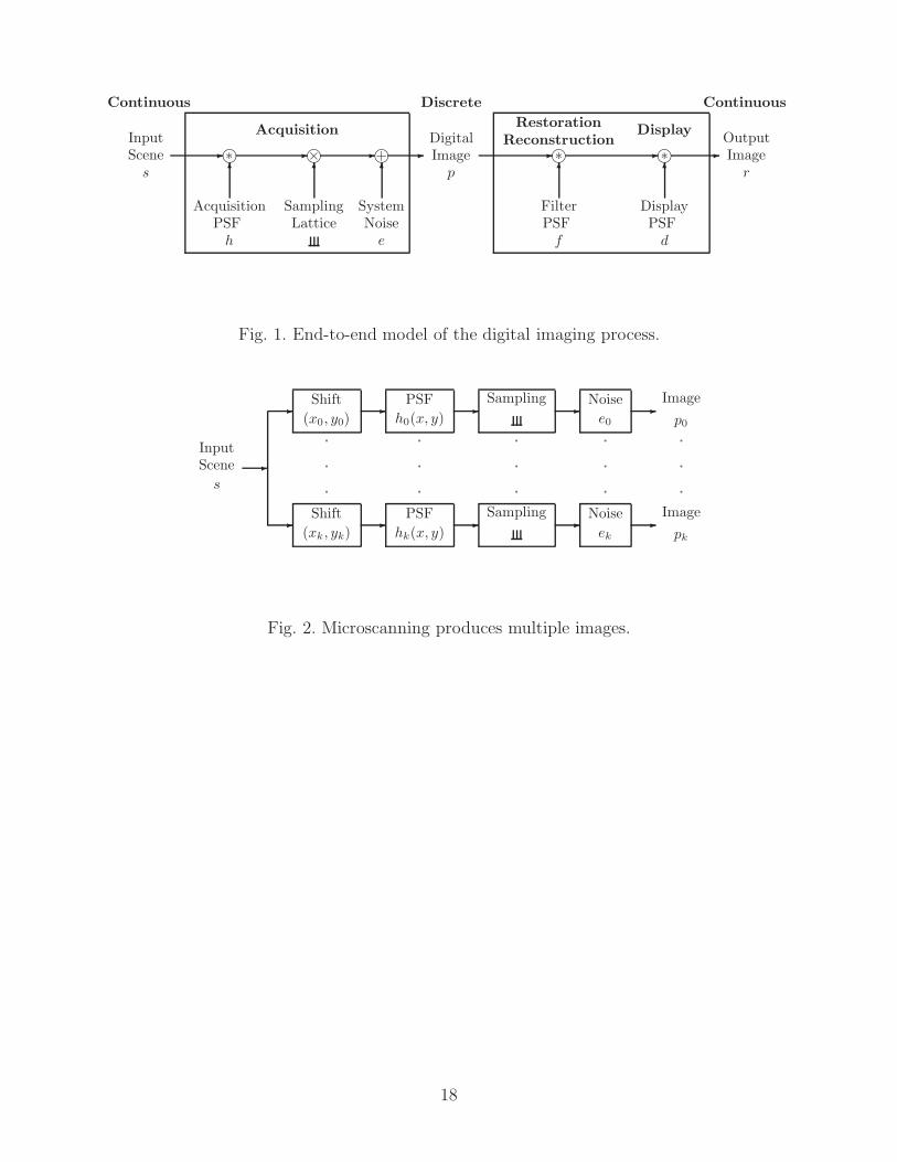
2. System Model and Problem Formulation

This section presents the CDC system model, describes microscanning, and formulates the

fidelity of a microscanning imaging system based on the system model. The system model

is introduced in the spatial domain of the image, but the problem and fidelity analysis are

formulated in the Fourier frequency domain so that spatial convolution can be considered as

pointwise multiplication of transform coefficients.

2.A. Continuous-discrete-continuous system model

The super-resolution methods developed in this paper are based on the CDC model pictured

in Fig. 1. This imaging system model is relatively simple, yet captures the most significant

degradations in typical imaging systems: linear shift-invariant blurring, characterized by the

acquisition point spread function (PSF) h; aliasing, due to sampling a continuous function

on a uniform, rectangular lattice ; additive system noise e; and display, characterized by

the display PSF d.

With this model, a single low-resolution digital image p is defined mathematically as:

p [m,n] =

∫ ∫s (x, y) h (m − x, n − y) dx dy + e [m,n] , (1)

where [m,n] are integer pixel indices for the digital image p and (x, y) are continuous coordi-

nates for the scene s. For notational convenience, and without loss of generality, the spatial

coordinates are normalized in units of the sampling interval. In practice, the spatial extent

of the image is finite, but that issue is not significant for the following analyses.

Restoration and reconstruction can be implemented in one step by convolving the image p

with the filter PSF f to produce a processed image of arbitrary resolution, which can then be

displayed. Modeling display as a linear shift-invariant process characterized by the display

PSF d, the resulting continuous output image r is:

r (x, y) =

∫ ∫ (∑

m

∑

n

p[m,n]f(x′ − m, y′ − n

))

d(x − x′, y − y′

)dx′ dy′. (2)

4

2.B. Microscanning

Microscanning is the process of generating multiple images from a common scene by shifting

either the scene or the image acquisition system. The shifting can be performed in a regular

pattern or irregular pattern. Fig. 2 illustrates the microscanning process for a sequence

of images pk, k = 0..K − 1, with unchanging scene shifted between images, variable blur

and noise, and fixed sampling grid. (Reverse shifting of the sampling grid for a fixed scene

produces the same images.) Then, microscanned image pk is:

pk [m,n] =

∫ ∫s (x − xk, y − yk)hk (m − x, n − y) dx dy + ek [m,n] , (3)

where k is the index for the microscanning image, (xk, yk) is the relative shift, hk is the

acquisition PSF, and ek is the additive system noise.

Image acquisition (with blurring, sampling, and noise), digital processing (for registration,

reconstruction, and restoration), and display of microscanned imaging is analyzed more easily

in the Fourier frequency domain, regardless of whether digital image processing is performed

in the spatial domain or the frequency domain. In the frequency domain, the Fourier trans-

form of the microscanned image pk (the transform of Eq. 3) is:

pk (u, v) =∑

µ

∑

ν

s (u − µ, v − ν) hk (u − µ, v − ν) exp−i2π((u−µ)xk+(v−ν)yk) + ek (u, v) , (4)

where ‘ ’ indicates the Fourier transform. In Eq. 4, the frequency-domain equivalent for

spatial-domain blurring by convolution in Eq. 3 is pointwise multiplication of the trans-

form coefficients of the scene and PSF. The frequency-domain equivalent for spatial-domain

sampling is the double sum, which folds the transform coefficients.

The microscanned images must be registered relative to one another. In the frequency

domain, the registered and combined microscanned images are:

p (u, v) =1

K

K−1∑

k=0

pk (u, v) expi2π(u(xk+αk)+v(yk+βk))

=1

K

∑

µ

∑

ν

s (u − µ, v − ν)

K−1∑

k=0

hk (u − µ, v − ν) expi2π(uαk+vβk)expi2π(µxk+νyk)

+1

K

K−1∑

k=0

ek (u, v) expi2π(u(xk+αk)+v(yk+βk)), (5)

where (αk, βk) is the registration error for image pk. Mathematically, the registered images

are combined by addition. If registration is perfect, then αk = βk = 0 and each microscanned

image is shifted to its proper position in the registered image.

In the Fourier frequency domain, reconstruction and restoration of the scene is the product

of the Fourier transform of the registered image p by the filter transfer function f . Then, the

display process multiplies that result by the display transfer function d:

r (u, v) = p (u, v) f (u, v) d (u, v) . (6)

5

2.C. Fidelity analysis

By Rayleigh’s Theorem, the expected mean square error (MSE) of the CDC imaging system

for an ensemble of scenes can be analyzed in either the spatial or frequency domain:

ǫ2 = E{∫ ∫

|r (x, y) − s (x, y)|2 dx dy

}

= E{∫ ∫

|r (u, v) − s (u, v)|2 dudv

}. (7)

The following analysis assumes that the power spectra of the scene ensemble and noise are

known, that the scene and noise are uncorrelated, that co-aliased components of the sampled

scene are uncorrelated, and that the noise between images is uncorrelated:24

E {s (u, v) s∗ (u − µ, v − ν)} =

{Φs (u, v) if (µ, ν) = (0, 0)

0 otherwise

E {ej (u, v) e∗k (u, v)} =

{Φek

(u, v) if j = k

0 otherwise

E {s (u − µ, v − ν) e∗k (u, v)} = 0 (8)

where the ‘*’ superscript denotes complex conjugation, Φs is the power spectra of the scene,

and Φekis the power spectra of the noise. For convenience, and without loss of generality,

scenes are normalized so that the mean and variance are zero and one respectively.

The expected MSE ǫ2 for the CDC imaging system can be expressed in terms of the scene

and noise power spectra, the acquisition transfer function, the relative shifts and registration

errors, the reconstruction and restoration filter, and the display transfer function:

ǫ2 =

∫ ∫ (Φs (u, v) − f (u, v) d (u, v) Φ∗

s,p (u, v) − f∗ (u, v) d∗ (u, v) Φs,p (u, v)

+∣∣∣f (u, v)

∣∣∣2 ∣∣∣d (u, v)

∣∣∣2Φp (u, v)

)dudv, (9)

where Φp is the power spectrum of the registered image and Φs,p is the cross-power spectrum

of the scene and the registered image:

Φp (u, v) = E{|p (u, v)|2

}

=1

K2

∑

µ

∑

ν

Φs (u − µ, v − ν)

∣∣∣∣∣

K−1∑

k=0

hk (u − µ, v − ν) E{

expi2π(uαk+vβk)expi2π(µxk+νyk)}∣∣∣∣∣

2

+1

K2

K−1∑

k=0

Φek(u, v)

Φs,p (u, v) = E {s (u, v) p∗ (u, v)}

= Φs (u, v)1

K

K−1∑

k=0

h∗k (u, v) E

{exp−i2π(uαk+vβk)

}. (10)

6

If the distribution of the registration errors is known, the expressions for expected MSE can

be analyzed with respect to those errors. For example, if αk and βk are uniformly distributed

on the intervals[− 1

2Wx, 1

2Wx

]and

[− 1

2Wy, 1

2Wy

]respectively, then observing:

∫ 1

2Wx

− 1

2Wx

∫ 1

2Wy

− 1

2Wy

expi2π(uαk+vβk) Wx Wy dαk dβk = sinc (u/Wx) sinc (v/Wy) , (11)

the components of the expected MSE are:

Φp (u, v) =1

K2sinc2 (u/Wx) sinc2 (v/Wy)

∑

µ

∑

ν

Φs (u − µ, v − ν)

∣∣∣∣∣

K−1∑

k=0

hk (u − µ, v − ν) expi2π(µxk+νyk)

∣∣∣∣∣

2

+1

K2

K−1∑

k=0

Φek(u, v)

Φs,p (u, v) = sinc (u/Wx) sinc (v/Wy) Φs (u, v)1

K

K−1∑

k=0

h∗k (u, v) . (12)

Φp is subject to the relative shifts (xk, yk). For instance, if the number of microscanned

images K is 2, Φp for relative shifts {(x0, y0) = (0, 0), (x1, y1) = (0, 0.5)} is the same as for

relative shifts {(x0, y0) = (0.5, 0), (x1, y1) = (0.5, 0.5)}, but is different than for relative shifts

{(x0, y0) = (0, 0), (x1, y1) = (0.5, 0)} and for {(x0, y0) = (0, 0.5), (x1, y1) = (0.5, 0.5)}. Filters

derived with respect to Φp can vary depending on the relative shift pattern of microscanned

images.

Fidelity25 is a normalized measure of image quality based on the MSE:

F = 1 − ǫ2∫ ∫Φs (u, v) dudv

. (13)

The greatest fidelity possible is 1, when the MSE is 0. The next section derives super-

resolution reconstruction and restoration filters that maximize fidelity F (or equivalently

minimize the MSE ǫ2).

3. Super-Resolution Reconstruction and Restoration

The techniques developed in this section are designed to perform reconstruction and restora-

tion. The methods take as input multiple images which have been registered and produce a

single output image with high fidelity and super-resolution.

3.A. CDC Wiener filter

For performance comparison, it is useful to derive the optimal CDC Wiener filter.24 Denoting

MSE as a functional of the filter transfer function f (u, v) yields:

ǫ2(f)

=

∫ ∫L(u, v, f

)dudv, (14)

7

where

L(u, v, f

)= Φs (u, v) − f (u, v) d (u, v) Φ∗

s,p (u, v) − f∗ (u, v) d∗ (u, v) Φs,p (u, v)

+∣∣∣f (u, v)

∣∣∣2 ∣∣∣d (u, v)

∣∣∣2Φp (u, v) . (15)

The optimal filter must satisfy:

∂L

∂f= f∗ (u, v)

∣∣∣d (u, v)∣∣∣2Φp (u, v) − d (u, v) Φ∗

s,p (u, v) = 0, (16)

so the optimal filter is:

fw (u, v) =Φs,p (u, v)

Φp (u, v)

d∗ (u, v)

|d (u, v) |2=

Φs,p (u, v)

Φp (u, v), (17)

where Φp and Φs,p are introduced to incorporate the effects of the display device on the

image (and are used in the derivations of the small kernels in the following sections). The

CDC Wiener filter cannot be implemented practically via spatial convolution because it is

continuous and its support is the full extent of the image. As described in the next section,

the computational costs of super-resolution reconstruction and restoration can be reduced

by constraining the spatial support of the filter to a small kernel.

3.B. Small-kernel Wiener filter

The derivation of the small-kernel Wiener filter fc is conditioned on constraints imposed on

its spatial support. The support of the kernel is a nonempty set of spatial discrete locations

C, for which filter values can be nonzero. Except for locations in the support set, the filter

value is 0:

fc (x, y) = 0, if (x, y) /∈ C. (18)

The larger the filter support, the better the performance, but small kernels can be highly

effective.26

The optimal, spatially constrained filter is derived by minimizing the MSE ǫ2 with respect

to the elements in C. Mathematically, it requires that:

∂ǫ2

∂fc (x, y)= 0 ∀(x, y) ∈ C. (19)

These constraints can be expressed in a system of linear equations:26

∑

(x′,y′)∈C

Φp

(x − x′, y − y′

)fc

(x′, y′

)= Φs,p (x, y) , ∀(x, y) ∈ C, (20)

where Φp is the auto-correlation of the displayed image and Φs,p is the cross-correlation of

the scene and the displayed image. The number of equations and the number of unknowns

are both equal to the number of elements in the support set C, i.e., there are |C| equations

in |C| unknowns.

8

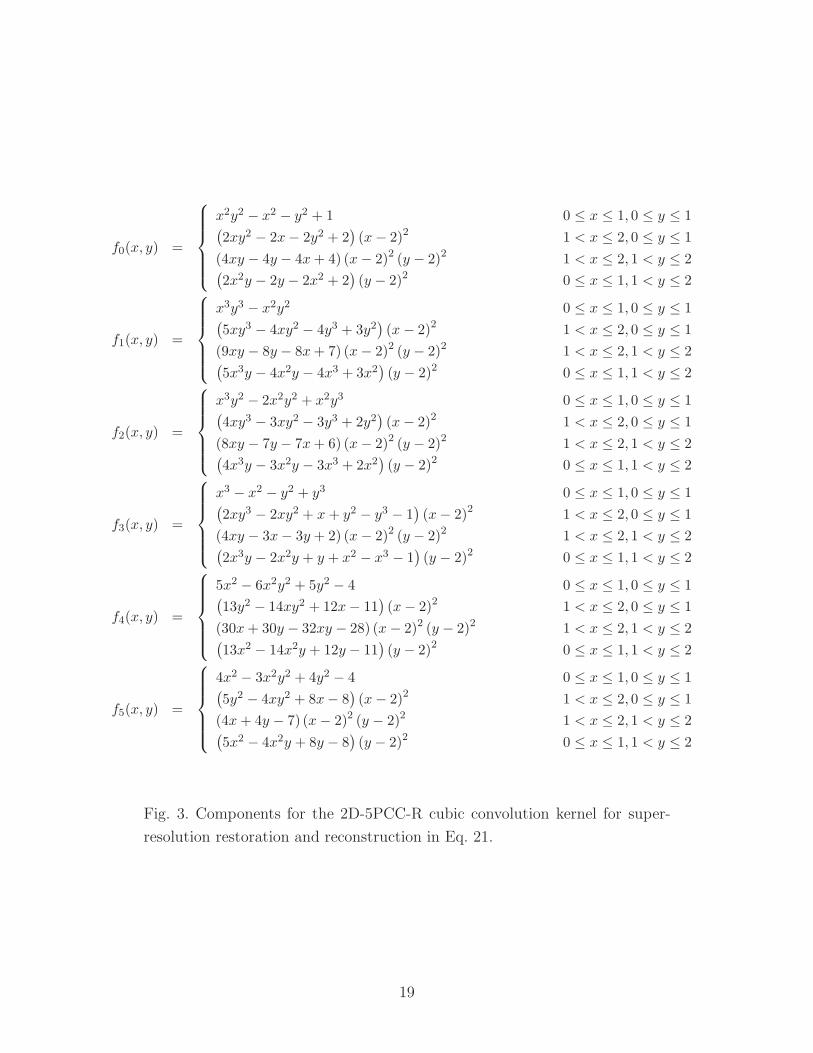
3.C. Parametric cubic convolution

Piecewise cubic convolution is a popular interpolation method for image reconstruction that

is traditionally implemented by separable convolution with a small one-dimensional kernel

consisting of piecewise cubic polynomials.27,28 This popular method can be generalized to

two dimensions and can be reformulated by relaxing constraints to perform reconstruction

and restoration in one-pass with small-kernel convolution.29 With constraints for symmetry,

continuity, and smoothness, the two-dimensional kernel with support [−2, 2] × [−2, 2] has

five parameters {a1, a2, a3, a4, a5}:

fp (x, y) = f0 (x, y) + a1f1 (x, y) + a2f2 (x, y) + a3f3 (x, y) + a4f4 (x, y) + a5f5 (x, y) , (21)

where f0–f5 are defined in Fig. 3. This kernel, designated 2D-5PCC-R (to distinguish it from

two-dimensional piecewise cubic interpolation30), is a continuous function.

The optimal 2D-5PCC-R kernel fp for an ensemble of scenes can be derived by minimizing

the MSE ǫ2 with respect to the five parameters. Computing the partial derivatives of ǫ2 with

respect to the parameters, and solving for simultaneous equality with zero:

∂ǫ2

∂a1=

∂ǫ2

∂a2=

∂ǫ2

∂a3=

∂ǫ2

∂a4=

∂ǫ2

∂a5= 0, (22)

yields five equations for the optimal parameter value:∫ ∫

fi (u, v)(Re{Φs,p (u, v)} − f0 (u, v) Φp (u, v)

)dudv

=

∫ ∫fi (u, v)

(fp (u, v) − f0 (u, v)

)Φp (u, v) dudv, i = 1..5. (23)

4. Experimental results

This section presents experimental results for a simulated imaging system and for real images.

In the simulation, the scene is a high resolution digital image. The simulated scene is blurred,

sampled, and degraded by noise (by digital processing) to produce simulated microscanned

images. These images are reconstructed and restored by the optimal CDC Wiener filter, the

small-kernel Wiener filter, 2D-5PCC-R, Shift-and-Add (with Wiener deconvolution, denoted

SA+Wiener),20,31 and Norm 2 Data with L1 Regularization (denoted Norm 2 Data).23,31

The super-resolution computations for the optimal Wiener filter are implemented in the

Fourier frequency domain by multiplying the filter defined in Eq. 17 by the Fourier transform

of the registered, combined images defined in Eq. 5. The computations for the small-kernel

Wiener filter and 2D-5PCC-R are implemented in the spatial domain, for computational

efficiency, by convolving the registered combined images with the small kernels defined by

the solutions for Eq. 20 and Eq. 23, respectively. Both SA+Wiener and Norm 2 Data were

developed at the Multi-Dimensional Signal Processing (MDSP) research lab at the University

9

of California at Santa Cruz.31 Norm 2 Data is an iterative super-resolution method and these

experiments use default parameter values (except the deconvolution kernel) of the software.

For simulated imaging, all resulting images are compared to the original scene. Because

the phase-shifts between the simulated scene and the microscanned images are known, the

simulation allows true quantitative measures of reconstruction and restoration performance.

The super-resolution methods also are applied to real images acquired by panning an infrared

camera slowly across a fixed scene. Because the true scene values are unknown, quantitative

evaluation is not possible. Also, the microscanning shifts must be estimated, so the results are

impacted by registration error. Nonetheless, real images are useful for qualitatively demon-

strating the effectiveness of the small-kernel methods in practice.

4.A. Simulation results

Fig. 4(A) illustrates a 256× 256 digital image acquired by aerial photography32 that is used

as a simulated scene and it is therefore the ideal super-resolution image. The simulated scene

is blurred by a Gaussian low-pass filter to simulate acquisition blurring:

h (u, v) = exp−(u2+v2), (24)

so the system transfer function at the Nyquist limit along each axis is h (0.0, 0.5) = h (0.5, 0.0)

= 0.779. After blurring, sixteen 64 × 64 low-resolution images are created with simulated

microscanning at quarter-pixel intervals along each axis. In each simulated microscanned

image, Gaussian white noise is added to each pixel so that the blurred-signal-to-noise ratio

(BSNR) is 30dB:

BSNR = 10 log10

(σ2

p/σ2e

), (25)

where σ2p is the variance of the blurred microscanned images (after blurring and before addi-

tive noise) and σ2e is the variance of the noise. Fig. 4(B) illustrates one of the microscanned

images (the reference image p0) interpolated back to 256×256 resolution by nearest-neighbor

interpolation to show the granularity of the sampling. Fig. 4(C) illustrates a higher quality

interpolation using cubic o-Moms.33 Four of the sixteen microscanned images are used for

deriving the reconstruction and restoration filters and for super-resolution processing:

× o × o

o o o o

× o × o

o o o o

,

where ‘×’ and ‘o’ respectively stand for locations (at quarter-pixel intervals) with and with-

out samples.

10

The actual scene power spectrum is used to derive the optimal CDC Wiener filter in

order to benchmark the optimal fidelity. The power spectrum for optimizing the small-kernel

Wiener filter and the 2D-5PCC-R filter, however, is estimated (as typically is required in

practice) using the power spectrum model of a two-dimensional isotropic Markov random

field (MRF).34 The model can be fitted to the image power spectrum30 or interactively

parameterized for visual quality (as done here). The MRF autocorrelation is:

Φs (x, y) = exp−√

x2+y2/ρ, (26)

where ρ is the mean spatial detail (MSD) of the scene in pixel units. MSD can be interpreted

as the average size of the details in the scene. In terms of the Hankel transform,35 the power

spectrum of the isotropic MRF is:

Φs (u, v) =2πρ2

(1 + 4π2ρ2(u2 + v2))3

2

. (27)

The CDC Wiener filter, small-kernel Wiener filter with support limited to [−2, 2] × [−2, 2],

and 2D-5PCC-R filter were derived for this simulation based on the isotropic MRF scene

model with MSD = 4 pixels. Fig. 5 illustrates the small-kernel Wiener PSF (in Fig. 5(A))

and the 2D-5PCC-R PSF (in Fig. 5(B)). The optimal parameter values for 2D-5PCC-R are

a1 = 74.176, a2 = −95.360, a3 = 16.804, a4 = −0.967, and a5 = 0.238.

Fig. 4(D)–(H) presents the simulation results for the super-resolution methods. To limit

boundary effects, the borders of all resulting images are cleared. Visually, the super-resolution

images produced by all of the restoration and reconstruction filters (in Fig. 4(D)–(H)) are

better than provided by a single frame (in Fig. 4(B)–(C)). For example, the small, lightly

colored rectangle in the upper-left quadrant between the diagonal runway and the left-most

vertical runway are clearer in the super-resolution images. The images produced by the five

super-resolution methods are of similar visual quality, but the CDC Wiener filter appears

to produce the best image and SA+Wiener appears to produce the worst image. The image

produced by the small-kernel Wiener filter appears to be slightly sharper than the image

produced by 2D-5PCC-R.

Table 1 lists the quantitative fidelity and computational costs for the various methods with

the simulation. The computational costs were measured in seconds, averaged over multiple

runs with MATLAB 6.5 Release 13 on a IBM R32 (Intel Pentium M 1.8GHz CPU, 256MB

RAM, MS Windows XP Professional 2002). The optimal CDC Wiener filter (which uses

the actual scene power spectrum) has the highest fidelity, as expected mathematically. The

CDC Wiener filter requires preprocessing to compute the filter (which then can be used

to filter multiple images) and requires forward and inverse Fourier transforms to apply the

filter. As expected, the image from cubic o-Moms with a single frame has the lowest fidelity.

The iterative method, Norm 2 Data, has fidelity nearly equal to the CDC Wiener filter, but

11

requires 50 iterations and nearly 50 seconds for Fig. 4(H). Of the three small-kernel filters

which can be efficiently applied by spatial convolution, the small-kernel Wiener filter has

somewhat higher fidelity than 2D-5PCC-R and SA+Wiener.

The visual and quantitative results for the simulation indicate that the small-kernel Wiener

filter and 2D-5PCC-R effectively improve image quality with efficient spatial-domain pro-

cessing.

CDC Wiener Small-kernel Wiener 2D-5PCC-R o-Moms SA+Wiener Norm 2 Data

Fidelity 0.980 0.975 0.966 0.928 0.966 0.979

Preprocessingtime (sec)

0.521 0.781 0.940 0.000 0.150 0.000

Filteringtime (sec)

0.121 0.030 0.030 0.120 0.380 49.121

Table 1. Fidelity and computational costs of various methods.

4.B. Results for real images

The super-resolution reconstruction and restoration methods require characterizations of

the system, including the noise power spectrum and acquisition transfer function. Noise

can be characterized accurately from flat-field calibration images or from regions of uniform

background of acquired images. The transfer function can be estimated to frequencies beyond

the Nyquist limit using a knife-edge technique with images for various sample-scene phase

shifts.36 Microscanning provides such images.

For this experiment with real images, the acquisition transfer function of an infrared

camera system was estimated from microscanned images of a four-bar target. The camera

platform was microscanned as low-resolution images were recorded. Fig. 6 illustrates a small

piece of one of the 256×256 low-resolution images from the microscanned sequence. Employ-

ing the super-resolution knife-edge technique,36 a sequence of 120 low-resolution images of

the bar target was registered with the subpixel accuracy (to 0.25 pixel) and averaged. Fig. 7

illustrates the resulting super-resolution horizontal slice across the four-bar targets, superim-

posed on the model of the bar target scene estimated by a thresholding the registered slice.

Fig. 8 illustrates the modulation transfer function (MTF) estimated by the CDC Wiener

filter. For this experiment, the two-dimensional acquisition transfer function was modeled as

the separable product of the one-dimensional estimate:

h(u, v) = hx(u)hx(v). (28)

12

A more accurate estimate of the two-dimensional acquisition transfer function could be made

from two or more slices.

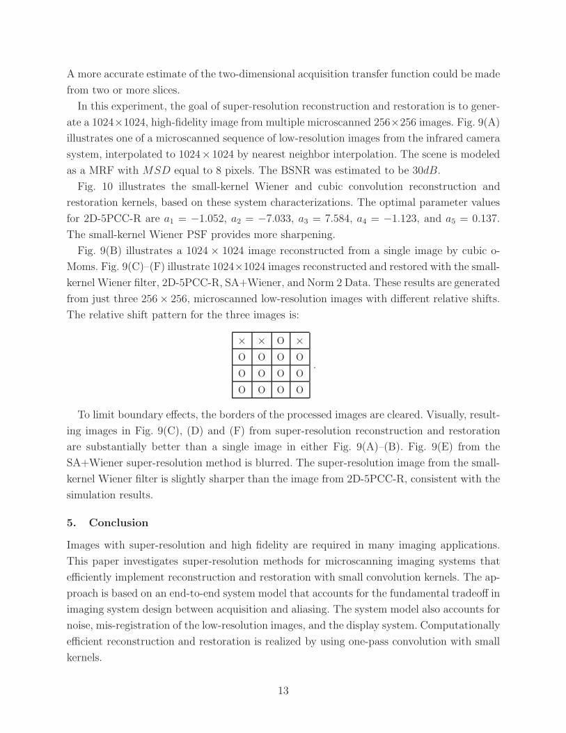
In this experiment, the goal of super-resolution reconstruction and restoration is to gener-

ate a 1024×1024, high-fidelity image from multiple microscanned 256×256 images. Fig. 9(A)

illustrates one of a microscanned sequence of low-resolution images from the infrared camera

system, interpolated to 1024×1024 by nearest neighbor interpolation. The scene is modeled

as a MRF with MSD equal to 8 pixels. The BSNR was estimated to be 30dB.

Fig. 10 illustrates the small-kernel Wiener and cubic convolution reconstruction and

restoration kernels, based on these system characterizations. The optimal parameter values

for 2D-5PCC-R are a1 = −1.052, a2 = −7.033, a3 = 7.584, a4 = −1.123, and a5 = 0.137.

The small-kernel Wiener PSF provides more sharpening.

Fig. 9(B) illustrates a 1024 × 1024 image reconstructed from a single image by cubic o-

Moms. Fig. 9(C)–(F) illustrate 1024×1024 images reconstructed and restored with the small-

kernel Wiener filter, 2D-5PCC-R, SA+Wiener, and Norm 2 Data. These results are generated

from just three 256× 256, microscanned low-resolution images with different relative shifts.

The relative shift pattern for the three images is:

× × o ×o o o o

o o o o

o o o o

.

To limit boundary effects, the borders of the processed images are cleared. Visually, result-

ing images in Fig. 9(C), (D) and (F) from super-resolution reconstruction and restoration

are substantially better than a single image in either Fig. 9(A)–(B). Fig. 9(E) from the

SA+Wiener super-resolution method is blurred. The super-resolution image from the small-

kernel Wiener filter is slightly sharper than the image from 2D-5PCC-R, consistent with the

simulation results.

5. Conclusion

Images with super-resolution and high fidelity are required in many imaging applications.

This paper investigates super-resolution methods for microscanning imaging systems that

efficiently implement reconstruction and restoration with small convolution kernels. The ap-

proach is based on an end-to-end system model that accounts for the fundamental tradeoff in

imaging system design between acquisition and aliasing. The system model also accounts for

noise, mis-registration of the low-resolution images, and the display system. Computationally

efficient reconstruction and restoration is realized by using one-pass convolution with small

kernels.

13

This paper develops two small convolution kernels for improved resolution and fidelity:

the spatially constrained Wiener filter and a parametric cubic convolution (designated 2D-

5PCC-R). Subject to constraints, both are optimized with respect to maximum end-to-end

system fidelity. Experimental results for a simulated imaging system and for real images

indicate the effectiveness of the small-kernel methods for increasing resolution and fidelity.

Visually, the super-resolution images from the small-kernel Wiener filter are slightly sharper

than images from 2D-5PCC-R, but both small-kernel methods yield significant quantitative

and qualitative improvements.

Additional work is required to develop efficient implementations of the small-kernel super-

resolution methods. Even with the efficiency of one-pass restoration and reconstruction

using small kernels, super-resolution processing requires significant processing. Each low-

resolution image pixel in the kernel’s region-of-support around each super-resolution pixel

contributes to the output value. Super-resolution processing of K images, with kernel sup-

port of [−S, S] × [−S, S] pixels and super-resolution increase of R × R, requires 4KS2R2

floating-point multiplications and additions (MADDs). If the distribution of low-resolution

pixels varies with respect to the super-resolution pixels, multiple kernels (each with KS2

weights) should be used in the computation. These issues make implementation, especially

in hardware, challenging.

References

1. M. G. Kang and S. Chaudhuri, “Super-resolution image reconstruction,” IEEE Signal

Processing Magazine 20(3), 19–20 (2003).

2. E. Choi, J. Choi, and M. G. Kang, “Super-resolution approach to overcome physical

limitations of imaging sensors: An overview,” International Journal of Imaging Systems

and Technology 14(2), 36–46 (2004).

3. S. C. Park, M. K. Park, and M. G. Kang, “Super-Resolution Image Reconstruction: A

Technical Overview,” IEEE Signal Processing Magazine 20(3), 21–36 (2003).

4. R. C. Hardie, K. J. Barnard, J. G. Bognar, E. E. Armstrong, and E. A. Watson, “High-

resolution image reconstruction from a sequence of rotated and translated frames and its

application to an infrared imaging system,” Optical Engineering 37(1), 247–260 (1998).

5. M. Elad and A. Feuer, “Restoration of a Single Superresolution Image from Several

Blurred, Noisy, and Undersampled Measured Images,” IEEE Transactions on Image

Processing 6(12), 1646–1658 (1997).

6. C. L. L. Hendriks and L. J. V. Vliet, “Improving Resolution to Reduce Aliasing in an

Undersampled Image Sequence,” SPIE 3965, 1–9 (2000).

7. H. Foroosh, J. B. Zerubia, and B. Marc, “Extension of Phase Correlation to Subpixel

Registration,” IEEE Transactions on Image Processing 11(3), 188–200 (2002).

14

8. M. Irani and S. Peleg, “Improving Resolution by Image Registration,” CVGIP: Graphical

Models and Image Processing 53(3), 231–239 (1991).

9. M. S. Alam, J. G. Bognar, R. C. Hardie, and B. J. Yasuda, “Infrared Image Registra-

tion and High-Resolution Reconstruction Using Multiple Translationally Shifted Aliased

Video Frames,” IEEE Transactions on Instrumentation and Measurement 49(5), 915–923

(2000).

10. T. M. Lehmann, C. Gonner, and K. Spitzer, “Survey: Interpolation Methods in Medical

Image Processing,” IEEE Transactions on Medical Imaging 18(11), 1049–1075 (1999).

11. M. L. Stein, Interpolation of Spatial Data: Some Theory for Kriging (Springer-Verlag,

New York, NY, 1999).

12. J. Ruiz-Alzola, C. Alberola-Lopez, and C. F. Westin, “Adaptive Kriging Filters for Mul-

tidimensional Signal Processing,” Signal Processing 85(2), 413–439 (2005).

13. A. K. Katsaggelos, Digital Image Restoration (Springer-Verlag, New York, NY, 1991).

14. R. L. Lagendijk and J. Biemond, “Basic Methods for Image Restoration and Identifica-

tion,” in Handbook of Image and Video Processing (A. Bovik, Ed. Academic Press,San

Diego CA, 2000).

15. M. K. Ng and N. K. Bose, “Mathematical analysis of super-resolution methodology,”

IEEE Signal Processing Magazine 20(3), 62–74 (2003).

16. R. Y. Tsai and T. S. Huang, “Multiframe Image Restoration and Registration,” in Ad-

vances in Computer Vision and Image Processing, pp. 317–339 (Greenwich, CT, 1984).

17. S. P. Kim, N. K. Bose, and H. M. Valenzuela, “Recursive Reconstruction of High Reso-

lution Image from Noisy Undersampled Multiframes,” IEEE Transactions on Acoustics,

Speech, and Signal Processing 38(6), 1013–1027 (1990).

18. S. P. Kim and W.-y. Su, “Recursive High-Resolution Reconstruction of Blurred Multi-

frame Images,” IEEE Transactions on Image Processing 2(4), 534–539 (1993).

19. R. R. Schultz and R. L. Stevenson, “Extraction of High-Resolution Frames from Video

Sequences,” IEEE Transactions on Image Processing 5(6), 996–1011 (1996).

20. M. Elad and Y. Hel-Or, “A Fast Super-Resolution Reconstruction Algorithm for Pure

Translational Motion and Common Space-Invariant Blur,” IEEE Transactions on Image

Processing 10(8), 1187–1193 (2001).

21. N. Nguyen and P. Milanfar, “A computationally efficient super-resolution image recon-

struction algorithm,” IEEE Transactions on Image Processing 10(4), 573–583 (2001).

22. S. Farsiu, D. Robinson, M. Elad, and P. Milanfar, “Advances and challenges in super-

resolution,” International Journal of Imaging Systems and Technology 14(2), 47–57

(2004).

23. S. Farsiu, D. Robinson, M. Elad, and P. Milanfar, “Fast and robust multiframe super

resolution,” IEEE Transactions on Image Processing 13(10), 1327–1344 (2004).

15

24. C. L. Fales, F. O. Huck, J. A. McCormick, and S. K. Park, “Wiener Restoration of

Sampled Image Data: End-to-End Analysis,” Journal of the Optical Society of America

A 5(3), 300–314 (1988).

25. E. H. Linfoot, “Transmission Factors and Optical Design,” Journal of the Optical Society

of America 46(9), 740–752 (1956).

26. S. E. Reichenbach and S. K. Park, “Small Convolution Kernels for High-Fidelity Image

Restoration,” IEEE Transactions on Signal Processing 39(10), 2263–2274 (1991).

27. R. G. Keys, “Cubic Convolution Interpolation for Digital Image Processing,” IEEE

Transactions on Acoustics, Speech, and Signal Processing 29(6), 1153–1160 (1981).

28. S. K. Park and R. A. Schowengerdt, “Image Reconstruction by Parametric Cubic Con-

volution,” Computer Vision, Graphics, and Image Processing 23, 258–272 (1983).

29. S. E. Reichenbach and J. Shi, “Two-dimensional Cubic Convolution for One-pass Im-

age Restoration and Reconstruction,” in International Geoscience and Remote Sensing

Symposium, pp. 2074–2076 (IEEE, 2004).

30. J. Shi and S. E. Reichenbach, “Image Image Interpolation by Two-Dimensional Para-

metric Cubic Convolution,” IEEE Transactions on Image Processing, to appear.

31. P. Milanfar, “Resolution Enhancement Software. www.soe.ucsc.edu/˜milanfar/SR-

Software.htm (2004)”.

32. Nebraska Department of Natural Resources, “Digital Orthophoto Quadrangle Database.

www.dnr.state.ne.us/databank/coq.html (2004)”.

33. T. Blu, P. Thevenaz, and M. Unser, “MOMS: maximal-order interpolation of minimal

support,” IEEE Transactions on Image Processing 10(7), 1069–1080 (2001).

34. R. A. Schowengerdt, Remote Sensing: Models and Methods for Image Processing, 2nd

ed. (Academic Press, Orlando, FL, 1997).

35. K. R. Castleman, Digital Image Processing (Prentice-Hall, Englewood Cliffs, NJ, 1979).

36. S. E. Reichenbach, S. K. Park, and R. Narayanswamy, “Characterizing Digital Image

Acquisition Devices,” Optical Engineering 30(2), 170–177 (1991).

16

List of Figure Captions

Fig. 1 End-to-end model of the digital imaging process.

Fig. 2 Microscanning produces multiple images.

Fig. 3 Components for the 2D-5PCC-R cubic convolution kernel for super-resolution restora-

tion and reconstruction in Eq. 21.

Fig. 4 Simulation results.

Fig. 5 The small reconstruction and restoration kernels for the simulation experiment.

Fig. 6 A low-resolution infrared image of a four-bar target used for estimating the acquisition

transfer function.

Fig. 7 Estimated acquisition transfer function hx(u).

Fig. 8 Estimated acquisition transfer function hx(u).

Fig. 9 Super-resolution results for a microscanned infrared system.

Fig. 10 The small reconstruction and restoration kernels for the real image experiment.

17

AcquisitionInputScene

s

Continuous

- h∗

AcquisitionPSF

h

6- h×

SamplingLattice

6- h+

SystemNoise

e

6-

DigitalImage

p

Discrete

Restoration

Reconstruction- h∗

FilterPSF

f

6-

Display

h∗6

DisplayPSF

d

OutputImage

r

-

Continuous

Fig. 1. End-to-end model of the digital imaging process.

InputScene

s

-

- Shift

(x0, y0)`

`

`

- Shift

(xk, yk)

- PSF

h0(x, y)`

`

`

- PSF

hk(x, y)

-Sampling

`

`

`

-Sampling

- Noise

e0

`

`

`

- Noise

ek

-Image

p0

`

`

`

-Image

pk

Fig. 2. Microscanning produces multiple images.

18

f0(x, y) =

x2y2 − x2 − y2 + 1 0 ≤ x ≤ 1, 0 ≤ y ≤ 1(2xy2 − 2x− 2y2 + 2

)(x − 2)2 1 < x ≤ 2, 0 ≤ y ≤ 1

(4xy − 4y − 4x + 4) (x − 2)2 (y − 2)2 1 < x ≤ 2, 1 < y ≤ 2(2x2y − 2y − 2x2 + 2

)(y − 2)2 0 ≤ x ≤ 1, 1 < y ≤ 2

f1(x, y) =

x3y3 − x2y2 0 ≤ x ≤ 1, 0 ≤ y ≤ 1(5xy3 − 4xy2 − 4y3 + 3y2

)(x − 2)2 1 < x ≤ 2, 0 ≤ y ≤ 1

(9xy − 8y − 8x + 7) (x − 2)2 (y − 2)2 1 < x ≤ 2, 1 < y ≤ 2(5x3y − 4x2y − 4x3 + 3x2

)(y − 2)2 0 ≤ x ≤ 1, 1 < y ≤ 2

f2(x, y) =

x3y2 − 2x2y2 + x2y3 0 ≤ x ≤ 1, 0 ≤ y ≤ 1(4xy3 − 3xy2 − 3y3 + 2y2

)(x − 2)2 1 < x ≤ 2, 0 ≤ y ≤ 1

(8xy − 7y − 7x + 6) (x − 2)2 (y − 2)2 1 < x ≤ 2, 1 < y ≤ 2(4x3y − 3x2y − 3x3 + 2x2

)(y − 2)2 0 ≤ x ≤ 1, 1 < y ≤ 2

f3(x, y) =

x3 − x2 − y2 + y3 0 ≤ x ≤ 1, 0 ≤ y ≤ 1(2xy3 − 2xy2 + x + y2 − y3 − 1

)(x− 2)2 1 < x ≤ 2, 0 ≤ y ≤ 1

(4xy − 3x− 3y + 2) (x − 2)2 (y − 2)2 1 < x ≤ 2, 1 < y ≤ 2(2x3y − 2x2y + y + x2 − x3 − 1

)(y − 2)2 0 ≤ x ≤ 1, 1 < y ≤ 2

f4(x, y) =

5x2 − 6x2y2 + 5y2 − 4 0 ≤ x ≤ 1, 0 ≤ y ≤ 1(13y2 − 14xy2 + 12x− 11

)(x − 2)2 1 < x ≤ 2, 0 ≤ y ≤ 1

(30x + 30y − 32xy − 28) (x − 2)2 (y − 2)2 1 < x ≤ 2, 1 < y ≤ 2(13x2 − 14x2y + 12y − 11

)(y − 2)2 0 ≤ x ≤ 1, 1 < y ≤ 2

f5(x, y) =

4x2 − 3x2y2 + 4y2 − 4 0 ≤ x ≤ 1, 0 ≤ y ≤ 1(5y2 − 4xy2 + 8x− 8

)(x − 2)2 1 < x ≤ 2, 0 ≤ y ≤ 1

(4x + 4y − 7) (x − 2)2 (y − 2)2 1 < x ≤ 2, 1 < y ≤ 2(5x2 − 4x2y + 8y − 8

)(y − 2)2 0 ≤ x ≤ 1, 1 < y ≤ 2

Fig. 3. Components for the 2D-5PCC-R cubic convolution kernel for super-

resolution restoration and reconstruction in Eq. 21.

19

A. 256 × 256 simulated scene B. Microscanned image C. Cubic o-Moms

D. CDC Wiener E. Small-kernel Wiener F. 2D-5PCC-R

G. SA+Wiener H. Norm 2 Data

Fig. 4. Simulation results: (A) the 256× 256 simulated scene and ideal super-

resolution image; (B) a single, 64 × 64, microscanned image reconstructed

to 256 × 256 with nearest-neighbor interpolation; (C) a single microscanned

image reconstructed to 256 × 256 with cubic o-Moms interpolation; (D)–(H)

super-resolution image restored and reconstructed to 256× 256 from four mi-

croscanned images by the CDC Wiener filter, small-kernel Wiener filter, 2D-

5PCC-R, SA+Wiener, and Norm 2 Data.

20

−2

−1

0

1

2

−2

−1

0

1

2

−1

0

1

2

3

4

5

6

7

8

−2

−1

0

1

2

−2

−1

0

1

2

−1

−0.5

0

0.5

1

1.5

2

2.5

3

3.5

A. Small-kernel Wiener filter B. 2D-5PCC-R

Fig. 5. The small reconstruction and restoration kernels for the simulation

experiment.

Fig. 6. A low-resolution infrared image of a four-bar target used for estimating

the acquisition transfer function.

21

10 20 30 40 50 60 70 80 90 100 110 120 130 140 150 1600

0.2

0.4

0.6

0.8

1

Horizontal index (1 unit = 0.25 pixel)

Val

ue o

f the

bar

targ

ets

RegisteredIdeal

Fig. 7. Super-resolution average scan of the bar target.

−2 −1.5 −1 −0.5 0 0.5 1 1.5

0.1

0.2

0.3

0.4

0.5

0.6

0.7

0.8

0.9

1

Fig. 8. Estimated acquisition transfer function hx(u).

22

A. 256 × 256 frame B. Cubic o-Moms

C. Small-kernel Wiener filter D. 2D-5PCC-R

E. SA+Wiener F. Norm 2 Data

Fig. 9. Super-resolution results for a microscanned infrared system.

23

−2

−1

0

1

2

−2

−1

0

1

2

−1

0

1

2

3

4

5

6

−2

−1

0

1

2

−2

−1

0

1

2

−1

0

1

2

3

4

A. Small-kernel Wiener filter B. 2D-5PCC-R

Fig. 10. The small reconstruction and restoration kernels for the real image

experiment.

24