arX

iv:a

stro

-ph/

0305

396v

2 2

2 M

ay 2

003

Astronomy & Astrophysics manuscript no. west˙arxive2 November 28, 2018(DOI: will be inserted by hand later)

Small-scale turbulent dynamo - a numerical investigation

R.J. West1, S. Nazarenko1, J.P. Laval2, and S. Galtier3

1 Mathematics Institute, University of Warwick, Coventry CV4 7AL, United Kingdom2 Laboratoire de Mecanique de Lille, CNRS, UMR 8107, Bld. Paul Langevin, 59655 Villeneuve d’Ascq Cedex,France

3 Institut d’Astrophysique Spatiale, Universite de Paris-Sud – CNRS, UMR 8617, bat. 121, 91405 Orsay Cedex,France

November 28, 2018

Abstract. We present the results of a numerical investigation of the turbulent kinematic dynamo problem in a highPrandtl number regime. The scales of the magnetic turbulence we consider are far smaller than the Kolmogorovdissipative scale, so that the magnetic wavepackets evolve in a nearly smooth velocity field. Firstly, we considerthe Kraichnan-Kazantsev model (KKM) in which the strain matrix is taken to be independent of coordinateand Gaussian white in time. To simulate the KKM we use a stochastic Euler-Maruyama method. We test thetheoretical predictions for the growth of rates of the magnetic energy and higher order moments (Kazantsev,1968; Kulsrud & Anderson, 1992; Chertkov et al., 1999), the shape of the energy spectrum (Kazantsev, 1968;Kulsrud & Anderson, 1992; Schekochihin et al., 2002a; Nazarenko et al., 2003) and the behaviour of the polari-sation and spectral flatness (Nazarenko et al., 2003). In general, the results appear to be in good agreement withthe theory, with the exception that the predicted decay of the polarisation in time is not reproduced well in thestochastic numerics. Secondly, in order to study the sensitivity of the KKM predictions to the choice of strainstatistics, we perform additional simulations for the case of a Gaussian strain with a finite correlation time and alsofor a strain taken from a DNS data set. These experiments are based on non-stochastic schemes, using a timestepthat is much smaller than the correlation time of the strain. We find that the KKM is generally insensitive tothe choice of strain statistics and most KKM results, including the decay of the polarisation, are reproduced well.The only exception appears to be the flatness whose spectrum is not reproduced in accordance with the KKMpredictions in these simulations.

Key words. Galaxies: magnetic fields – ISM: magnetic fields – Magnetic fields – Methods: numerical – MHD –Turbulence

1. Introduction

Many astrophysical magnetic fields are believed to be gen-erated via a dynamo action (Moffatt, 1978; Parker, 1979;Childress & Gilbert, 1995) in systems where the magneticfield diffusivity κ is much less than that of the kinematicviscosity ν. These systems correspond to large magneticPrandtl number Pr = ν/κ flows. Such astrophysical situ-ations are observed in the interstellar medium as well as inprotogalactic plasma clouds where the magnetic Prandtlnumber varies respectively from Pr ∼ 1014 to Pr ∼1022 (Chandran, 1998; Kulsrud, 1999; Schekochihin et al.,2002a). Such high values of Pr lead to an interesting in-terval of scales (from 7 to 11 decades in our examples)below the viscous cut-off, but above the magnetic diffu-sive scale, where magnetic fluctuations are stretched by arandomly changing smooth velocity field. The small-scale

Send offprint requests to: S. Nazarenko,snazar@maths.warwick.ac.uk

kinematic dynamo problem can thus be formulated as towhether a small initially “seeded” magnetic field, subjectto stretching by a prescribed smooth velocity field, willgrow in time.

One can picture the evolution of an ensemble of mag-netic wavepackets, each traveling together with the fluidparticles which are distorted by the local strain. By as-suming a given form of the strain statistics, an idealisedhomogeneous and isotropic strain that is a Gaussian whitenoise process, one can simplify the problem, leading to aproductive framework from which analytical results canbe obtained. This formalism is known as the Kraichnan-Kazantsev model (KKM) (Kraichnan & Nagarajan, 1967;Kazantsev, 1968). It should be remembered that such amodel is a simplification and a real turbulent velocityfield will exhibit finite correlations of the fluid velocityfield, as well as being to some degree non-Gaussian, inho-mogeneous and anisotropic. Therefore, in this numerical

2 R.J. West et al.: Small-scale turbulent dynamo

investigation we will also consider more realistic examplesof the velocity field.

The work presented here is based on a kinematicmodel, making use of the linear induction equation of themagnetic field B(x, t)

DtB = B · ∇v + κ∇2B, (1)

where Dt ≡ ∂t + v · ∇ is the material derivative, v thevelocity, and κ the magnetic diffusivity. Physically, wecan have in mind the following picture for the evolutionof our dynamo system. Initially, for small κ, the B-fieldwill be “frozen” into the flow behaving as a passive vec-tor field (Soward, 1994). After some period of time, andhence growth of the magnetic field, diffusion will becomeimportant and will reduce this rate of growth. In partic-ular, using the KKM the growth of the total mean mag-netic energy < B2(t) > was obtained by Kazantsev (1968)and that of the higher order moments < B2n(t) > byChertkov et al. (1999). Schekochihin et al. (2002a) haveextended this work to include the effects of compressibil-ity.

The work presented here has two primary aims. Thefirst aim is to numerically verify the analytical scal-ing laws found by Kazantsev (1968) and Chertkov et al.(1999) for the even moments < B2n(t) > (where n isa positive integer) in both the perfect conductor (non-diffusive) and diffusive regimes. We will also compute theFourier space one-point correlators which have recentlybeen investigated analytically (Schekochihin et al., 2002a;Nazarenko et al., 2003). In the past much emphasis hasbeen placed solely on investigations of the magnetic energyspectrum. However, higher order correlators are also ofsignificance. Indeed, they describe statistics of the fluctua-tions around the mean energy distributions in the Fourierspace. Also, it has been shown that the new quantities,the mean polarisation of the magnetic turbulence and thespectral flatness, are of particular interest as they char-acterise the properties of the small-scale intermittency(Nazarenko et al., 2003). These newer theoretical objectswill also be investigated numerically. Our second aim is tostudy the sensitivity of the dynamo model to the choice ofstrain statistics. In a quest to test the universality of theanalytical results found using the KKM, we will considerthe case of a finite-correlated Gaussian strain field. We willalso consider a more realistic strain field generated from aDirect-Numerical-Simulation (DNS) of the Navier-Stokesequations.

The presentation of this paper has been organised intosix main sections. In the next section we give a brief in-troduction to the small-scale dynamo problem, with asummary of the KKM analytical results as derived byChertkov et al. (1999) and Kazantsev (1968). In the thirdsection we outline some of the new KKM analytical re-sults in regard to the behaviour of the one-point Fourierspace correlators; a more detailed discussion of which canbe found in Nazarenko et al. (2003). The fourth sectionprovides an overview of the numerical method used toinvestigate the KKM and its subsequent results. In the

fifth section we outline the method and results of thefinite-correlated Gaussian and DNS based investigations.Finally, we draw our conclusions in the sixth section.

2. Moments of B

Let us briefly summarise the analytical results forthe moments of B(t) obtained within the KKM byChertkov et al. (1999). At scales below the viscous cut-off Batchelor (Batchelor, 1950, 1954) argued the velocityfield would be random and smooth (Batchelor regime). InMHD a uniform velocity cannot alter a system’s magneticfield. The flow

vi = σijxj , (2)

where σ(t) is a coordinate independent random strain ma-trix, represents one of the simplest choices of a velocityfield that allows for the transfer of kinetic energy into mag-netic energy (Zel’dovich et al., 1984). The incompressibil-ity condition ∇·v = 0 in this case corresponds to Tr[σ] =0 for all time. It is natural to reformulate our mathemati-cal description in terms of Lagrangian dynamics (namelyfollowing particles) in which case Dt ≡ d/dt in the induc-tion equation (1). Zel’dovich et al. (1984) (Soward, 1994)showed that given an initial condition, the induction equa-tion (1) can be re-written in Fourier space as

B(k, t) = J(t)B(q, 0) exp

(

−κ

∫ t

0

k2(t′)dt′)

, (3)

where the Jacobian J(t) satisfies

d

dtJ = σJ, (4)

with the initial condition J(0) = I, with I the unit matrix,and q = k(0) is the initial wavevector related to k(t) by

q = JTk. (5)

Moments of B are calculated via two independent averag-ings, one over initial statistics, and the other over variousrealisations of the strain matrix (Chertkov et al., 1999).The initialB field is assumed to be homogeneous, isotropicand Gaussian, with zero mean and the following variance

< Ba(k, 0)Bb(k′, 0) > = (6)

(

δab −kakbk2

)

k2Eme−k2L2

δ(k − k′),

where L is the length-scale at which the “seed” magneticnoise is initially concentrated and Em is a constant whichdetermines the initial turbulence intensity. After averagingover the initial statistics Chertkov et al. (1999) obtainedthe following expression for B2(t)

B2(t) =

∫

Eme−q2L2

e−2κqΛq q2 Jia

(

δab −qaqbq2

)

Jib dq, (7)

with summation over repeated indices and where q = |q|and Λ(t) satisfies

Λ(t) =

∫ t

0

dt′ J−1(t′)J−T (t′). (8)

R.J. West et al.: Small-scale turbulent dynamo 3

The full even moments < B2n(t) > where calculated bytaking the value of B2 to the correct power and then av-eraging over the realisations of the velocity field. For anisotropic, delta-correlated, Gaussian strain field

< σab(t)σab(0) > = 10λ1δ(t), (9)

where λ1 is the growth rate of a material line element, cor-responding to the largest Lyapunov exponent of the flow,Chertkov et al. (1999) derived the following expressionsfor the scaling behaviour of the even moments< B2n(t) >.In the perfect conductor regime t < 3td/(2n+3), we have

< B2n(t) > ≃ e2λ1n(2n+3)t/3, (10)

where on dimensional grounds the scale at which mag-netic diffusion becomes important is rd ≃

√

κ/λ1 and thecorresponding time is td ≃ λ−1

1 ln(L/rd). In the diffusiveregime t > 3td/(n+ 2), we have

< B2n(t) > ≃ eλ1n(n+4)t/4. (11)

For n = 1, this result was derived earlier by Kazantsev(1968).

3. Fourier Space Correlators

Traditionally, Fourier space analysis of the dynamoproblem has only really involved investigations ofthe k-space correlator corresponding to the energyspectrum E(k, t) =< |B(k)|2 > (Kazantsev, 1968;Kulsrud & Anderson, 1992; Schekochihin et al., 2002a).Kazantsev (1968) studied the dynamo system as aneigenvalue problem from which he was able to obtainthe growth exponents of the total magnetic energy.The evolution of the energy spectrum in k-space hasalso been studied both analytically and numerically byKulsrud & Anderson (1992).

In this KKM analysis, the way in which we define theincompressible strain matrix is different to (9) used inChertkov et al. (1999). We write

σij√Ω

= Gij −Tr[G]

3δij (12)

where G is a 3 × 3 matrix made up of independentGaussian N(0; 1) random variables, normally distributed(i.e. Gaussian) with zero mean and a standard deviationof 1, such that

< Gij(t)Gkl(0) >= δikδjlδ(t). (13)

This choice is motivated by its convenience in numericalmodelling. One should note there is a degree of flexibilityin how we define our strain statistics, a more detailed dis-cussion of which can be found in the appendix. The KKMresults remain the same for different choices of the strainstatistics, the only difference being that time is re-scaledby a constant factor.

3.1. Energy Spectrum

3.1.1. Energy Spectrum : κ = 0 Solution

In the limit of zero diffusion κ = 0, the 3D energy spec-trum has the solution (Nazarenko et al., 2003)

E(k, t) =E0√t

(

k

q

)−1/2

exp

(

−3 ln2(k/q)

4Ωt

)

exp

(

5Ωt

4

)

, (14)

where q is the wavenumber at which E(k) is initially con-centrated at t = 0, and E0 is a constant depending onthe initial conditions. If we let td be the diffusion timeas defined in section 2 or Chertkov et al. (1999), then forlarge time Ω−1ln2(k/q) ≪ t ≪ td, i.e. in the perfect con-ductor regime, we have E ∼ k−1/2. Alternatively, we canthink of the k−1/2 slope as being present over an intervalof wavenumber space kc− ≪ k ≪ kc+ where

kc±(t) ∼ exp(±√

4Ωt/3). (15)

The critical wavenumbers kc+ and kc− govern when theexponential log squared term above becomes important.We see the fronts at kc+ and kc− propagate exponentiallyin time, and within this k−1/2 range the spectrum alsogrows exponentially. By integrating equation (14), overthe whole of wavenumber space, one can obtain the growthrate of the total magnetic energy

< B2(t) >=

∫

E(k, t) dk ≃ const exp(10Ωt

3). (16)

which agrees with result (10) for n = 1 when we take intoaccount the slightly different definitions of the strain co-variance. Indeed, one finds that the λ1t of (10) and Ωt of(16) are equivalent if we re-scale time by a factor of 4/5.Hence the scaling laws of Chertkov et al. (1999), presentedin section 2, for the diffusive regime should be re-writtenfor our choice of strain statistics as

< B2n(t) > ≃ e2nΩ(2n+3)t/3. (17)

Further, in the diffusive regime we have

< B2n(t) > ≃ eΩn(n+4)t/4. (18)

3.1.2. Energy Spectrum : κ 6= 0 Solution

If all wavevectors are initially of the same length|q|, and we are interested in large time asymptotics(Schekochihin et al., 2002a; Nazarenko et al., 2003), thesolution in the diffusive regime takes the form

E(k, t) ≃ const e5Ωt/4k−1/2t−3/2K0(k/kκ), (19)

where K0 is a MacDonald function of zeroth order and kκis a constant given by kκ =

√

Ω/6κ. In fact this kκ is thewavenumber at which diffusion becomes important. It istherefore equivalent to the estimated kd ∼ 1/rd derivedon purely dimensional grounds in section 2.

4 R.J. West et al.: Small-scale turbulent dynamo

3.2. Flatness and Polarisation

Although the energy spectrum solutions described aboveprovides us with some very useful information, they do notprovide us with a complete picture of our system. In therecent work of Nazarenko et al. (2003) higher one-pointcorrelators of the magnetic field in Fourier space werestudied1. In this paper, as well as for the energy spectrumE(k, t), we will also study two other correlators

S(k, t) =< |B(k)|4 >, (20)

T (k, t) =< |B2(k)|2 > . (21)

Let us briefly review the results from Nazarenko et al.(2003) regarding these correlators.

3.2.1. Polarisation Spectrum and Flatness : κ = 0Solutions

In the perfect conductor regime, the fourth ordercorrelators of Fourier amplitudes S ≡< |B(k)|4 > andT ≡< |B2(k)|2 > have exact solutions

S(k, t) =1√t

(

k

q

)1/2

exp

(

−3 ln2(k/q)

4Ωt

)

(22)

[

V0 exp

(

21Ωt

4

)

+3

7Q0 exp

(

−3Ωt

4

)]

,

T (k, t) =1√t

(

k

q

)1/2

exp

(

−3 ln2(k/q)

4Ωt

)

(23)

[

V0 exp

(

21Ωt

4

)

− 4

7Q0 exp

(

−3Ωt

4

)]

,

where V0 and Q0 are constants. In large time the Q0 termscan be neglected and these spectra develop a k1/2 scalingbetween two propagating fronts kc− ≪ k ≪ kc+.

Combining these two fourth order correlators, we findan important new quantity P = (S − T )/S, the physicalsignificance of which becomes clear when we write P as

P =4

< |B|4 >

∑

i6=j

< (ℑBiB∗j )2 >= (24)

4

< |B|4 >

∑

i6=j

< |Bi|2|Bj |2 sin2(φi − φj) >,

where φi is the phase of the complex component Bi andthe operator ℑ· takes the imaginary part of an expres-sion. In this form we see that P contains information aboutthe phases of the k-space modes. P can be thought of asthe mean normalised polarisation. Indeed, P = 0 corre-sponds to the plane polarisation of the Fourier modes. In

1 These were objects of the form < |B|2n|B2|2m > whichrepresent a basis for all one-point correlators in magnetic tur-bulence which is isotropic.

contrast for a Gaussian magnetic field one finds the polar-isation P = 1/3. Combining (22) and (23), in large timewe find the normalised polarisation P evolves as

P =Q0

V0exp(−6Ωt). (25)

That is, the polarisation is independent of wavenumber kand decays exponentially. This solutions tells us that inthe perfect conductor regime, the Fourier modes of themagnetic field will eventually become plane polarised. Incomparison, we should recall a Gaussian field has a finitepolarisation, thus our turbulent magnetic field is far frombeing Gaussian.

Another important measure of turbulent intermittencyin a fluid, both in real and Fourier space, is the flatness.The spectral flatness is defined as the ratio

F =S

E2=

< |B(k)|4 >

< |B(k)|2 >2. (26)

Using (26), one finds a Gaussian field has a constant flat-ness of 3/2. On the other hand small-scale intermittencycorresponds to a field with a flatness that grows both intime and in wavenumber space. Indeed, in the perfect con-ductor regime, the magnetic field displays such small-scaleintermittent behaviour (Nazarenko et al., 2003), with

F ∼ t1/2 exp

(

11Ωt

4

)

k3/2 exp

(

3 ln2(k/q)

4Ωt

)

. (27)

For kc− < k < kc+, we see there is a range of k3/2 scaling,while for larger k there is an increase in the flatness arisingfrom the log-squared exponential term. This intermittencyin Fourier space can be attributed to the presence of co-herent structures, as will be discussed later.

3.2.2. Polarisation Spectrum and Flatness : κ 6= 0Solutions

In the diffusive regime the fourth order correlators S andT have large time solutions (Nazarenko et al., 2003)

S ≃ k1/2t−3/2

[

V0e21Ωt/4 +

3

7Q0e

−3Ωt/4

]

K0

(

k

kκ,2

)

, (28)

T ≃ k1/2t−3/2

[

V0e21Ωt/4 − 4

7Q0e

−3Ωt/4

]

K0

(

k

kκ,2

)

, (29)

where kκ,2 =√

Ω/12κ. This kκ,2 can again be interpretedas the wavenumber at which diffusion becomes important.However, in comparison to the energy spectrum we shouldnote that the spectral cut-off will be at a smaller wavenum-ber as kκ,2 < kκ. Importantly we see that the normalisedpolarisation (25) behaves identically in both the diffusiveand perfect conductor regimes. In contrast, the behaviourof the flatness is modified

F =S

E2≃ k3/2t3/2e11Ωt K0(k/kκ,2)

(K0(k/kκ))2, (30)

R.J. West et al.: Small-scale turbulent dynamo 5

when compared to (27). For small k, we again have a re-gion of k3/2 scaling but now with a log correction aris-ing from the MacDonald functions. For large k, below thespectral cut-off, the additional MacDonald functions actto heighten the flatness. That is, the introduction of afinite diffusivity actually increases the small-scale inter-mittency.

4. KKM Numerical Investigation

The key to modelling the KKM numerically is the suc-cessful integration of equation (4) to find J . As the strainmatrix on the right hand side of (4) contains noise, itis evident that this is not a normal ordinary differentialequation (ODE) and should instead be interpreted in thestochastic sense. Following the analytical formalism (12)and (13), the elements of the strain matrix σ will be madeup from a matrix of Gaussian random variables G, suchthat the incompressibility condition Tr[σ] = 0 is satis-fied. As with any stochastic formalism one must decidethe form of the integral. Mathematically both the Ito andStratonovich definitions of the stochastic integral are cor-rect. It is only in a few special cases that both interpreta-tions produce the same solutions. In the present problemthis is not the case. Indeed, the Stratonovich formalism isthe correct interpretation for our problem as we are us-ing white noise as an idealisation of what in reality is acoloured noise process (Kloeden et al., 1997).

The simplest numerical scheme one can use to solveStochastic Differential Equations (SDE) is called theEuler-Maruyama scheme (EMS), and it can be thoughtof as generalisation of the normal forward Euler method(Kloeden et al., 1997). The stochastic numerical experi-ments presented here can be divided into two separateimplementations. Both these codes require the stochas-tic integration of the J equation (4), which we performnumerically using an EMS. Averaged quantities are cal-culated over many realisations of the strain statistics andinitial conditions. An ensemble of particles is chosen as theinitial condition, randomly distributed on a unit sphere inwavenumber space |q| = 1 (corresponding to an isotropicdistribution in real space). Each particle is subjected toits own realisation of the strain matrix, and its wavevectorevolves according to equation (5).

4.1. Code 1

Using the integration process described above for the evo-lution matrix J , Code 1 (C1) determines how the magneticfield evolves according to equation (7). As each particle issubjected to its own realisation of the strain matrix theintegral (7) over initial conditions simplifies to just thevalue of the integrand. Higher order quantities, such asB4 · · ·, can then be calculated before performing the finalaveraging over strain statistics. The initial magnetic noiseis determined by (6) with L = 1 . In the case of κ 6= 0

one must also determine the value of the matrix Λ(t) fromequation (8). This is achieved via a forward Euler scheme.

Λjk(tn+1) = Λjk(tn) +t

(

3∑

l=1

J−1jl (tn)J

−Tkl (tn)

)

. (31)

We see therefore, that we must also determine the valueof J−1. This can be done in two different ways. Firstly,we could calculate the inverse of J at each step in theusual manner by finding the adjoint and determinant ofJ . However, as some elements of J can become very largein time one needs to be careful in finding the determinantas round-off errors can be easily introduced. Alternatively,we can integrate the separate stochastic equation for theevolution of J−1

d

dt(J−1) = −(J−1)σ, (32)

using an EMS.The primary aim of this code is to verify the scaling

laws for the even moments < B2n(t) >, (17) and (18).However, by recording the values of the integrand of (7)and the corresponding wavenumbers k = |k| for each par-ticle, we can also construct snapshots of the energy spec-trum in time.

C1 has also been set up to calculate the eigenvaluesof the matrix JJT so that the Lyapunov exponents canbe calculated. Indeed, one important result for systemswith random time-dependent strain is that, for nearlyall realisations of the strain, the matrix (1/t) ln(JT J) isfound to stabilise at large time (Goldhirsch et al., 1987;Falkovich et al., 2001). The eigenvectors fi in this casetend to a fixed orthonormal basis for each realisation,where i = 1, 2, 3. As the Jacobian J at t = 0 is the iden-tity matrix, JT J will also take the form of the identityinitially. In time the strain σ will distort J via (4). An ini-tial sphere will be deformed into an ellipsoid, the volume ofwhich will be conserved by the incompressibility conditionDet[J ] = 1. The length of the principal axis of the ellipsoidcorrespond to the eigenvalues e2ρi of JTJ , while the eigen-vectors fi give the directions of these axis. It is evident thatin considering a time-dependent stochastic strain we havemoved to a system corresponding to Lagrangian chaos. Inwhich case, we can define the Lyapunov exponents λi interms of the limiting eigenvalues (Goldhirsch et al., 1987;Soward, 1994; Falkovich et al., 2001) as

λi = limt→∞

1

2tln(fTi (JT J)fi), (33)

for i = 1, 2, 3. It is customary to order the Lyapunov expo-nents in terms of size, λ1 > λ2 > λ3. A material elementaligned along one of the eigenvectors fi will in the asymp-totic limit expand or contract at the rate exp(λit). TheLyapunov exponents do not depend on the realisations ofthe strain, while in contrast the asymptotic eigenvectorsare realisation dependent. Incompressibility ensures that∑3

i=1 λi = 0 which in turn tells us that one Lyapunovexponent must be positive if two or more are non-zero. A

6 R.J. West et al.: Small-scale turbulent dynamo

positive Lyapunov exponent corresponds to exponentialgrowth of a material line element.

In the non-degenerate case, if the statistics of thestrain matrix are symmetric to time reversal, which istrue if the strain is assumed delta correlated as is thecase for the KKM, then λ2 = 0 (Kraichnan, 1974;Balkovsky & Fouxon, 1999) and hence the incompressibil-ity condition gives λ3 = −λ1 < 0. Chertkov et al. (1999)found that it is the largest Lyapunov exponent λ1 that isresponsible for the growth of the moments < B2n(t) >.Balkovsky & Fouxon (1999) have also considered the ma-trix JJT , which evolves in time according to

d

dt(JJT ) = σ(JJT ) + (JJT )σT . (34)

This differs to the matrix JTJ in that it does not stabiliseto some fixed axis at large time. Indeed, the eigenvectorswill continue to rotate for every realisation of the strainmatrix. As in (33), the Lyapunov exponents can also befound from the logarithm of the eigenvalues of JJT atlarge time. The eigenvalues of JJT and JT J , and hencetheir Lyapunov exponents, are the same as they share thesame characteristic polynomial.

To determine the Lyapunov exponents of our systemnumerically we need to determine either JJT or JTJ ateach timestep. This can be achieved by either calculatingJJT via its own dynamic equation (34) and integrate itusing an EMS, or alternatively calculate JJT or JTJ ateach timestep from J . In practice either approach worksequally well. Next one must determine the eigenvalues ofthe symmetric matrix JJT which must be real. Althoughthe matrix is only 3× 3 solving the characteristic polyno-mial using the solution to a cubic equation is impracticalas the growth/reduction of elements J in time produceround-off errors numerically. This in turn leads to com-plex eigenvalues and further inaccuracies.

The method employed in this numerical study is thatof Jacobi transformations (Press et al., 1993). The key tothis method is a sequence of similarity transformations(rotations). In the context of ellipsoids, this algorithm canbe thought of as a method by which the axis of the sys-tem are rotated and re-aligned to lie along the principleaxis of the ellipsoid, the length of these axis correspond-ing to the eigenvalues, and the directions to the eigen-vectors. Although the Jacobi rotation method is not per-fect, it does however perform better than the previouslymentioned cubic equation approach, in that the eigenval-ues remain real for all time. Given the set of eigenvaluesexp(2ρi) of JJ

T , we define the time-dependent Lyapunovexponents to be

λi(t) =1

2t< ln(exp(2ρi)) >=

1

t< ρi >, (35)

where i = 1, 2, 3. Analytically the Lyapunov exponentsare independent of the strain realisations at large time,but the averaging above has been performed over all therealisations and initial conditions to improve accuracy.

4.1.1. κ = 0 simulations

We will start by setting κ = 0 in the numerics so that wecan investigate the perfect conductor regime. Firstly, letus compare the scaling of < B2(t) > with theoretical so-lution (17). The left-hand graph of Fig. 1 corresponds tothe n = 1 case and we see the numerically generated slopeagrees nicely with the theoretical scaling (dashed line).For the higher order moments < B2n(t) >, good agree-ment with the analytical scaling (17) can also be seen.The right-hand graph in Fig. 1 shows the slope for n = 2.As all moments are calculated from the integral (7), itshould be noted that any fluctuations in B2(t) will get am-plified at higher orders, consequently the resulting graphswill become progressively noisier. The only solution to thisproblem is to increase the number of the realisations overwhich averaging is performed.

Let us now investigate the energy distribution inwavenumber space. The energy spectrum < B2(k, t) > isobtained at a particular instant in time by recording eachparticles wavenumber k = |k| and “weight” correspondingto the integrand of (7). One then constructs a histogramby first finding the largest and smallest wavenumbers kmax

and kmin of the all the particles, and then dividing the in-terval log kmin < log k < log kmax into a finite numberof bins. Particles are then sorted into these bins and theircorresponding weights are summed. Finally, we normalisethe total weight in each bin, by dividing through by its binwidth. One must also divide through by a factor of 4πk2

which originates from the solid angle integration requiredin converting a 1D spectrum into that of a 3D one (see forexample McComb (1990)).

In Fig. 2 the energy spectrum has been plotted for twodifferent times t = 9 (left figure) and t = 18 (right figure).Here Ω = 0.16 and thus using the definition (15) for thecritical wavenumber kc+(t) we obtain log10 kc±(9) = ±0.6and log10 kc±(18) = ±0.85. In Fig. 3 the same spectrumhas been plotted for t = 27 (left figure) and t = 31.5(right figure), correspondingly log10 kc+(27) = 1.04 andlog10 kc+(31.5) = 1.13. One should recall that theoret-ically for wavenumbers kc− ≪ k ≪ kc+ we expect ak−1/2 scaling range2, and this is indeed the case here(the straightline in each graph corresponding to a slopeof k−1/2). As a whole we can see that the spectrum movesvertically upwards in time. This corresponds to the timedependent increase of the magnetic energy at fixed kpredicted in the theoretical result (14). This large timeasymptotic solution has also been plotted on each figureand we see good agreement with the numerically gener-ated histograms.

It should be noted that the later figures show the spec-trum for log10 k > 0. This is because the front propa-gating to small k becomes extremely noisy at large time.The reason for this will become apparent shortly. It isevident from these results that it would be beneficial if

2 Here, we are considering a 3D spectrum.Kulsrud & Anderson (1992) considered the equivalent1D spectrum which has a corresponding k

3/2 scaling regime.

R.J. West et al.: Small-scale turbulent dynamo 7

we could extend the number of decades over which thisscaling is observed. A possible approach would be to runthe simulations for a much longer time, remembering thatlog kc±(t) ∼

√Ωt. In doing this one has to be careful of

numerical stability and the generation of round-off errorsas some elements of J will get ever larger. However, this isnot the only problem, we should remember that our dis-tribution of particles, initially concentrated at our initialwavenumber |q| = 1, will broaden in time. The peak ofthis distribution will move towards larger k, each individ-ual particle performing its own random walk in wavenum-ber space. Fig. 4 shows the distribution of particles atfour successive times t = 9, 18, 27 and 35 for a simula-tion with Ω = 0.16. The graph has been normalised sothat the area under the curve is one. We see that withlog wavenumber coordinate, the particle distribution fitsa moving Gaussian profile. The mean of this profile movesto higher wavenumbers as Ωt, while the standard devi-ation grows as

√Ωt. Regrettably, the energy spectrum’s

k−1/2 scaling range of interest lies in one of the tails ofthe particle distribution. This means that there will befewer particles available for averaging when calculatingthe energy spectrum histogram in this region.

The only way to improve this averaging is to increasethe total number of particles used in a simulation. Ofcourse, this is not an efficient way of improving the statis-tics, as increasing the number of rarer particles locatedin each tail, will correspond to a much greater increase inthe number of particles located in the centre of the particledistribution. This is an inherent problem with this type ofparticle simulation. Also, as the particle distribution getsmore spread out in time, fluctuations at both ends of theenergy spectrum histogram will increase. This effect canclearly be seen in Fig. 2 and 3. That is why the front kc−that propagates to smaller k < q < 1 in time becomes sonoisy, as the bulk of the particles are travelling to largerwavenumbers. For this reason in the remaining results wewill concentrate only on the log10 k ≥ 0 region of k-space.

4.1.2. κ 6= 0 simulations

We will now introduce a non-zero κ into the numericalmodel to investigate the effects of diffusion. The first thingwe will investigate here is the scaling behaviour of the totalmagnetic energy < B2(t) > in the diffusive regime. Theleft-hand graph of Fig. 5 shows the results of a simulationwith Ω = 0.36 and κ = 0.005. The two separate scalingregimes are clearly apparent and the analytical slopes (17)and (18), for the perfect conductor and diffusive regimesrespectively, are in good agreement with the numerics. Itis inevitable that to generate similarly smooth graphs forthe higher order moments, one would have to use a greaternumber of realisations. Figure 6 and the right-hand graphof Fig. 5 show the scaling of the next three even moments.As expected these graphs are noisier, but still in agreementwith the analytical results.

Next we will consider the energy spectrum. The in-troduction of a finite diffusivity will cut-off the energyspectrum at some finite wavenumber. Figure 7 shows twosuccessive snapshots of the energy spectrum at times t = 6and 12 for a simulation with κ = 0.005 and Ω = 0.36. Asexpected, one observes a spectral cut-off and for the resultsshown in Fig. 7, the parameter choice gives kκ =

√

Ω/6κ.Theory predicts that for k < kκ there should be a re-gion of k−1/2 scaling (19) (with a logarithmic correction).For this particular simulation we have log10 kκ ≃ 1.1. Aswith the perfect conductor regime, the spectrum is seento move vertically upwards corresponding to a steady in-crease in the total magnetic energy. The large time the-oretical solution (19) has also been plotted in Fig. 7 andgood agreement is observed.

We will briefly review the Lyapunov exponents gener-ated in these C1 numerical experiments because it helpus to understand the origins of some numerical errors inour method. Using the Jacobi transform method describedearlier, one can calculate the eigenvalues e2ρi from eitherJTJ or JJT , and then order them in terms of size sothat ρ1 > ρ2 > ρ3. The Lyapunov exponents are thendetermined via (35). Figure 8 shows < 2ρ1(t) > for a sim-ulation with Ω = 0.36. As expected the graph tends to aflat line in time, and λ1 > 0. We would expect λ1 ∼ Ω,that is < ln e2ρ1 >= 2tλ1 = 2tCΩ where C is the time-scaling constant mentioned earlier. In Fig. 8 a line corre-sponding to C = 4/5 has also been plotted. From theorywe would expect the remaining two Lyapunov exponentsto take the values λ2 = 0 and λ3 = −λ1, with conser-vation of volume corresponding to

∑

λi = 0. The leftand right-hand graphs of Fig. 9 shows < 2ρ2(t) > and< 2ρ3(t) > respectively. Looking at the range of the verti-cal axis we see λ2 does indeed stay around zero but thereis a gradual deviation from the theoretical value in time.On the other hand, λ3 is not the same as −λ1. The line< ln e2ρ3 >= −2tλ1 = −2tCΩ with C = 4/5 has also beenplotted for comparison. Numerically, we see that

∑

λi 6= 0and hence, according to the Lyapunov exponents, the vol-ume is not conserved. It should also be mentioned that inour simulations, the determinant of the Jacobian Det[J ],is held within 1% of unity, which means that the volumeis well conserved. We conclude therefore that the devia-tions observed in the numerical values of λi from theoryare mainly due to errors generated in finding the eigen-values of JJT or JTJ using the Jacobi transform method.This is not overly surprising if we remember that someelements of JJT are very large in comparison to others.Indeed, that is why the alternative method of finding theeigenvalues via solving the cubic characteristic polynomialof JJT runs into difficulties. In the context of the ellip-soids, essentially the problem arises because each ellipsoidis becoming ever larger in one direction and smaller inanother.

It should be noted that the magnetic Reynolds num-ber is relatively small in these simulations. The magneticReynolds number is by definition Rm =

√

L2Ω/κ, giv-ing a range of values 32 to 72 in the above simulations,

8 R.J. West et al.: Small-scale turbulent dynamo

where we have taken L to be of unity. Thus, it is onlythe relative sizes of Ω and κ that are important. HigherReynold number simulations are possible but again in-creasing Ω will make the stochastic fluctuations greaterand hence one will need to reduce the timestep in eachsimulation. Alternatively, decreasing the diffusivity κ willdelay the time at which the second regime commences. Inwhich case, the corresponding simulation will have to berun over a larger time interval.

4.2. Code 2

Code 2 (C2) uses the same foundations as C1, an ensembleof particles are initially distributed on the surface of a unitsphere in wavenumber space. However, now each particleis given a randomly orientated magnetic field satisfyingB · q = 0. That is, the real and imaginary parts of themagnetic field are randomly orientated in a plane whichis at right-angles to the particle’s initial wavevector andtangent to the unit sphere in k-space. Particles are againallowed to evolve in wavenumber space via (5), but incontrast to C1, information about the full magnetic fieldis retained by the integration of equation (3). In the caseof κ 6= 0 we need to determine the integral in (3). As withC1 this is achieved through the use of a forward Eulerscheme. In this way one can investigate the spectra ofFourier space quantities of interest such as the magneticenergy, polarisation and flatness.

4.2.1. κ = 0 simulations

Starting with the energy spectrum < B2(k, t) >. This hasbeen plotted in the left-hand graph of Fig. 10 along withthe large time theoretical curve (14) and slope k−1/2, forthe choice of parameters Ω = 0.16 and t = 35. As withthe C1 experiment Fig. 3, the numerical and analyticalresults support each other well. As with the investigationof higher order moments < B2(t) > in section 4.1.1, thehigher order correlators, such as S =< |B|4(k, t) >, willgenerate noisier histograms in comparison to their lowerorder counterparts. Nevertheless, the following numericalresults are still very much of interest. Firstly, we will ex-amine the correlator S which has been plotted as the right-hand graph of Fig. 10. The large time asymptotic solutionshas also been plotted, and there appears to be good quali-tative agreement with the numerics, although some devia-tion is evident at large k. As with the energy spectrum theanalytical results tell us that there exists a k+1/2 scalingrange for k < kc+. In this simulation log10 kc+ = 1.13. Aslope of k+1/2 has been included in the graph and againthere would seem to be agreement. However, it must besaid that the k-interval for this scaling range is perhapstoo short and the histogram too noisy to be conclusive.

For the same simulation, Fig. 11 shows the normalisedmean polarisation P (left figure) and spectral flatnessF (right figure). Let us consider the P spectrum. Fromthe theoretical results we expect P to be independent

of wavenumber. Although, the histogram is noisy, theredoes indeed appear to be no k-dependence, and the re-sulting spectra is flat. However, for the KKM we alsohave the prediction that the polarisation tends to zero intime (25). Unfortunately, this is not the case numerically.Indeed, taking an average over all k in the histogram wecan find an approximate value for P from the above spec-trum. Repeating this procedure for various snapshots intime we find the normalised polarisation remains steady intime at the value of 0.32. One should remember that for aGaussian field analytically we found P = 1/3. Therefore,in our numerical simulation the polarisation seems to bethat of a Gaussian field. However, the corresponding spec-tral flatness is far from being Gaussian. Indeed, the flat-ness F in this perfect conductor simulation can be seen inthe right-hand graph of Fig. 11. Below log10 kc+ = 1.13 wesee agreement with the analytical solution of k+3/2. Whileat larger k the theoretical increase in the flatness, due tothe log squared term in (27), is also well represented.

One may well ask, why is there a discrepancy betweentheory and the numerically generated polarisation, but notthe flatness? It helps if we can understand the physical sig-nificance of these two quantities. We return to the familiarexample of the evolution of an initial ball of isotropic mag-netic turbulence is wavenumber space. For each realisationthis ball is deformed into an ellipsoid with one large, oneshort and one neutral direction. One can visualise this el-lipsoid as an elongated flat cactus leaf with thorns alignedto the magnetic field direction. Note that in this pictureone component of the magnetic field (transverse to thecactus leaf) is dominant which is captured by the factthat the polarisation P introduced above, tends to zero atlarge time. Another consequence of this picture is that thewavenumber space will be covered by the ellipsoids moresparsely at large k. This produces large intermittent fluc-tuations of the Fourier transformed magnetic field. Thesefluctuations are quantified by the growth of the flatness Fas k3/2, a clear indication of this small-scale intermittency.

Numerically, it would appear that the flatness is a littlemore robust than the polarisation, arising naturally in thenumerics as the ellipsoids become increasingly sparse atlarge k. In contrast, the apparently Gaussianity of thepolarisation can be attributed to the mis-alignment of thecactus needles. Indeed, the magnetic needles should alignthemselves with the smallest principal axis of the ellipsoid.In this direction the cactus leaf is becoming continuouslythinner in time, and hence numerically one might expectsome errors to creep into the alignment of B. Indeed, thisseems to be related to the errors observed in calculatingthe smallest Lyapunov λ3.

In fact, although on average our numerical simulationsappear to mis-represent the behaviour of the polarisationcompletely, things are not as bad as they would initiallyseem. Indeed, further insight can be obtained by consid-ering the behaviour of an ensemble of particles that aresubjected to the same realisation of the strain. Figure 12shows the real magnetic fields of a set of 500 wavepacketsthat have been subjected to two different realisations of

R.J. West et al.: Small-scale turbulent dynamo 9

the strain matrix3. In the left-hand figure it is clear themagnetic field in this realisation is far from being planepolarised, the magnetic vectors still being predominantlyrandom in their orientation at this given point in timet = 6. In contrast, in the right-hand figure, which hasalso been taken at t = 6, we see the ellipsoid has becomevery elongated and the magnetic field appears plane po-larised. Earlier snapshots, at t = 2 and 5, of the magneticfield for this particular realisation can be found in Fig.13, and the evolution of the corresponding polarisationspectra is shown in Fig. 14. In this case, we see the po-larisation does indeed decay in time and is far from beingGaussian by t = 6. In some respects, therefore, our numer-ical model does get some of the polarisation’s behaviourat least qualitatively correct.

Before we consider the effects of finite diffusivity, weshould check how the growth rates of the spectra behavein time. That is, how rapidly they move vertically up ordown in time. By recording the value of each spectra fork = 1, at different snapshots in time, we can comparethis numerical growth to the theoretical solutions (14),(22), (23) and (27) for E, S, T and F respectively. Theseresults can be found in Fig. 15. Along with the numeri-cal values (points) the corresponding theoretical growthhas also been plotted (solid line). It should be noted thatthis is only a rough check. Firstly, because we have hadto ignore the

√t prefactor in each analytic solution, and

secondly because the numerical values of the spectra atk = 1 are likely to fluctuate at large time as we are againin the tails of the particle distribution. Nevertheless, allthe spectra are growing in time in agreement with theory.

4.2.2. κ 6= 0 simulations

In this section we will discuss the results of a set of C2simulations with a finite diffusivity of κ = 0.005. Figure 16shows snapshots of < B2(k, t) > at the times t = 6 and 12.As with the C1 simulations, the finite diffusivity producesa spectral cut-off. As expected the spectrum moves verti-cally upwards in time, with the second histogram gettingnoiser as the density of particles in the interval k < kc+ isreduced. Comparing these energy spectra to their equiva-lent C1 counterparts, Fig. 7, we should note that the C2numerics appear to be slightly hyper-diffusive. This effectis most probably numerical, originating from the integra-tion of the k2 integral found in (3).

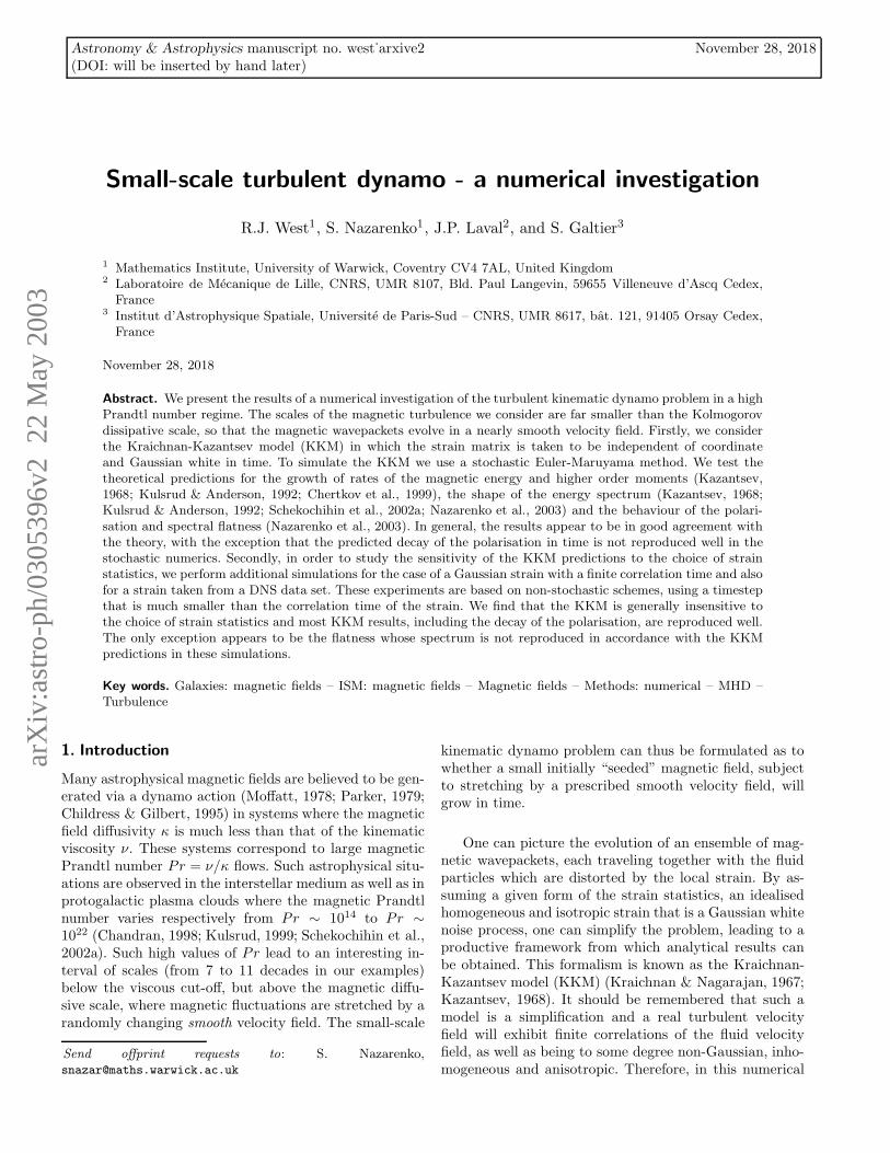
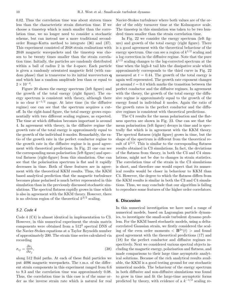
The higher order correlators S and T have been plot-ted in Fig. 17 for a time t = 6. We should note that theparticles here have been sorted into 100 bins. However,the axis in each graph has been re-scaled to take into ac-count the spectral cut-off. For small k, qualitatively thesefigures are in agreement with the large time asymptoticsolutions. However, as with the energy spectrum, theseresults seem to slightly hyper-diffusive. The final figurewe will consider is 18 which shows flatness F at t = 6.

3 The imaginary magnetic fields are qualitatively similar andhave therefore not been included.

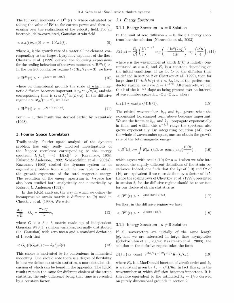
Again we observe good qualitative agreement with the-ory. In particular, one can observe a k3/2 scaling region forsmall k and a heightened flatness at larger k in agreementwith equation (30). This coincides with the analytical pre-diction that the inclusion of a finite diffusivity increasesthe flatness (and hence small-scale intermittency) at largek. The corresponding normalised mean polarisation spec-trum has not been included here as it is again flat, muchlike the perfect conductor regime (see Fig. 11) but witha spectral cut-off. As with the non-diffusive case, on av-erage the normalised polarisation appears Gaussian withP = 0.32. Again, it is interesting to consider the magneticfield of an ensemble of particles that have been subjectedto the same realisation of the strain matrix. Figure 19shows two such snapshots of an ensemble of 500 magneticparticles. These two figures should be compared with Fig.12 which show the same realisations but without diffusion.The right-hand figure in particular demonstrates why, inthe diffusive regime, an ellipsoid will cover k-space moresparsely due to the decay of its magnetic field at its tips.This is the reason why spectral flatness increases in thediffusive regime.

5. Numerical Investigations Beyond the KKM

The purpose of the stochastic codes outlined above was toinvestigate the small-scale dynamo system for the case of aGaussian white strain field. In contrast, the following twocodes were developed to test the universality of the ana-lytical KKM results summarised in section 3, when morerealistic representations of the velocity field are chosen.These simulations are based on the integration of the in-duction equation (1), which when written in a Lagrangianframe of reference in k-space4 takes the form

d

dtBm = σmiBi − κk2Bm, (36)

where d/dt ≡ ∂t + kj∂kjand

kj = −σijki. (37)

Numerically we consider an ensemble of particles(wavepackets), whose individual magnetic fields evolve ac-cording to (36) and wavevectors according to (37).

5.1. Code 3

In code 3 (C3), we consider a synthetic Gaussian strainfield with a finite correlation time. The r.m.s. of the dif-ferent strain components in this numerical experimentranged from 2.9 to 3.6 and the correlation time was

4 Strictly speaking, the Fourier transforms used in derivingthis equation must be taken over a box. The box size is greaterthan the characteristic length-scale of magnetic turbulence, butless than the characteristic length-scale of the velocity field. Inthis case, model (2) corresponds to ignoring the quadratic (inx) terms in the scale separation parameter. The strain here ismeasured along the fluid path.

10 R.J. West et al.: Small-scale turbulent dynamo

0.02. Thus the correlation time was about sixteen timesless than the characteristic strain distortion time. If wechoose a timestep which is much smaller than the corre-lation time, we no longer need to consider a stochasticscheme, but can instead use a more traditional second-order Runge-Kutta method to integrate (36) and (37).This experiment consisted of 2048 strain realisations with2048 magnetic wavepackets and the timestep was cho-sen to be twenty times smaller than the strain correla-tion time. Initially, the particles are randomly distributedwithin a ball of radius 2 in the k-space. Each particleis given a randomly orientated magnetic field (with ran-dom phase) that is transverse to its initial wavevectors qand which has a random amplitude less than or equal to2× 10−4.

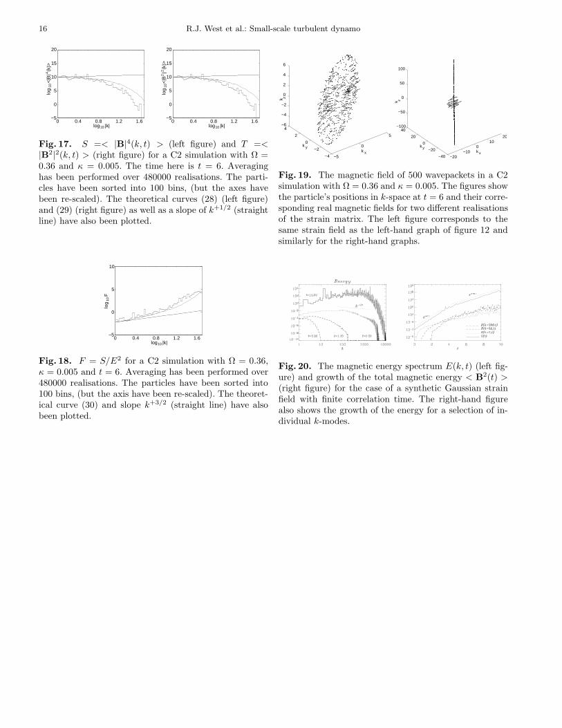
Figure 20 shows the energy spectrum (left figure) andthe growth of the total energy (right figure). The en-ergy spectrum is consistent with theory, although thereis no clear k−1/2 range. At later time (in the diffusiveregime) one can see that the spectrum acquires a cut-off. In the right-hand figure, the total energy grows expo-nentially with two different scaling regimes, as expected.The time at which diffusion becomes important is around4. In agreement with theory, in the diffusive regime thegrowth rate of the total energy is approximately equal tothe growth of the individual k-modes. Remarkably, the ra-tio of the growth rate in the perfect conductor regime tothe growth rate in the diffusive regime is in good agree-ment with theoretical predictions. In Fig. 21 one can seethe corresponding mean polarisation (left figure) and spec-tral flatness (right-figure) from this simulation. One cansee that the polarisation spectrum is flat and it rapidlydecreases in time. Both of these features are in agree-ment with the theoretical KKM results. Thus, the KKMbased analytical prediction that the magnetic turbulencebecomes plane polarised is much better represented in thissimulation than in the previously discussed stochastic sim-ulations. The spectral flatness rapidly grows in time whichis also in agreement with the KKM theory. However, thereis no obvious region of the theoretical k3/2 scaling.

5.2. Code 4

Code 4 (C4) is almost identical in implementation to C3.However, in this numerical experiment the strain matrixcomponents were obtained from a 5123 spectral DNS ofthe Navier-Stokes equations at a Taylor Reynolds numberof approximately 200. The strain time series calculated viarecording

σij =∂vi∂xj

, (38)

along 512 fluid paths. At each of these fluid particles weput 4096 magnetic wavepackets. The r.m.s. of the differ-ent strain components in this experiment ranged from 6.6to 9.3 and the correlation time was approximately 0.08.Thus, the correlation time in this case is of the same or-der as the inverse strain rate which is natural for real

Navier-Stokes turbulence where both values are of the or-der of the eddy turnover time at the Kolmogorov scale.The timestep in this simulation was taken to be two hun-dred times smaller than the strain correlation time.

In Fig. 22 we consider the energy spectrum (left fig-ure) and growth of the total energy (right figure). Thereis a good agreement with the theoretical behaviour of theenergy spectrum. One can see a region of k1/2 scaling anda log correction in the diffusive regime. Note that the purek1/2 scaling changes to the log-corrected spectrum at thetime when the high-k tail hits the dissipative scale whichapproximately corresponds to the third curve in Fig. 22measured at t = 0.44. The growth of the total energy isagain well represented. The growth rate exponent changesat around t = 0.4 which marks the transition between theperfect conductor and the diffusive regimes. In agreementwith the theory, the growth of the total energy the diffu-sive regime is approximately equal to the growth of theenergy found in individual k modes. Again the ratio ofthe growth rates in the perfect conductor and the diffu-sive regimes is consistent with theoretical predictions.

The C4 results for the mean polarisation and the flat-ness spectra are shown in Fig. 23. One can see that themean polarisation (left figure) decays in time and is spec-trally flat which is in agreement with the KKM theory.The spectral flatness (right figure) grows in time, but theshape of the spectrum is different from the theoretical re-sult of k3/2. This is similar to the corresponding flatnessresults obtained in C3 simulations. In fact, the deviationsof the flatness from theory, in both the C3 and C4 simu-lations, might not be due to changes in strain statistics.The correlation time of the strain in the C3 simulationsis short, and therefore one would expect that its numer-ical results would be closer in behaviour to KKM thanC4. However, the degree to which the flatness differs fromthe KKM results is similar in both the C3 and C4 simula-tions. Thus, we may conclude that our algorithm is failingto reproduce some features of the higher order correlators.

6. Discussion

In this numerical investigation we have used a range ofnumerical models, based on Lagrangian particle dynam-ics, to investigate the small-scale turbulent dynamo prob-lem. For the KKM based stochastic models, using a delta-correlated Gaussian strain, we firstly considered the scal-ing of the even order moments < B2n(t) > and foundgood agreement with the theoretical predictions (17) and(18) for the perfect conductor and diffusive regimes re-spectively. Next we considered various spectral objects in-cluding the magnetic energy, polarisation and flatness, andmade comparisons to their large time asymptotic analyt-ical solutions. Because of the rich analytical results avail-able, the KKM is a good testing ground for our stochasticnumerical models. The behaviour of the energy spectrumin both diffusive and non-diffusive simulations was foundto grow in time and fit the large-time asymptotic formspredicted by theory, with evidence of a k−1/2 scaling re-

R.J. West et al.: Small-scale turbulent dynamo 11

gion in each case. The fourth order correlators were alsoconsidered. Although noisier than the energy spectrum,these spectra also appeared consistent with the analyt-ical results. However, there was evidence of some hyper-diffusion in these numerical results are high wavenumbers.The new analytical objects, the mean polarisation andspectral flatness, were investigated. The flatness was wellbehaved with an observed k3/2 scaling and the growthrate in time in agreement with the analytical predictions.In contrast, the polarisation of the magnetic turbulencein these simulations was mis-represented. Although it wasspectrally flat, in agreement with the theory, it appearedto saturate at its Gaussian value of 1/3 rather than de-caying in time. However, on considering individual real-isations it was apparent that at least some of the pre-dicted decaying behaviour was observed qualitatively inthese simulations. This also provided us with a useful vi-sualisation of the dynamo system in terms of a cactus leafin k-space. The linear polarisation corresponds to the k-space alignment of the magnetic field “thorns” along thedirection of the smallest Lyapunov exponent, i.e. trans-verse to the cactus leaf pad. The flatness growth with kis directly linked to the fact that at larger k the cactusleaves will cover the k-space more sparsely. We also com-puted the Lyapunov exponents and found that the largestexponent was well represented which ensures the correctgrowth of the total magnetic energy. The behaviour of thesmallest exponent was badly reproduced, which may beconnected to the observed behaviour of the polarisation.

A second set of experiments was also performed totest the universality of the KKM based theoretical re-sults with respect to changes in the strain statistics. Thesetwo simulations, used a finite-correlated Gaussian and aDNS generated strain fields respectively. For the finite-correlated Gaussian strain based model, the energy spec-trum was found to be consistent with theory, although nok−1/2 scaling region could clearly be distinguished. Forthe DNS strain based model there was an agreement withtheory for both the growth rate of the total energy andthe k−1/2 scaling. Remarkably, these two numerical exper-iments demonstrated excellent agreement with the theo-retical behaviour of the polarisation, in each case beingboth spectrally flat and decaying in time. Also in agree-ment with the theory is the rapid time growth of the flat-ness. In contrast, the spectral shape of the flatness in thesesimulations was not as well represented as in the stochas-tic based results. For both the finite-correlated Gaussianand DNS strain based simulations the flatness spectrumwas far from the predicted k3/2 scaling. We believe thisdifference from theory is a numerical artifact from our al-gorithm, rather than directly due to changes in the formof the velocity field. We conclude that the gross featurespredicted by the KKM theory seem to be robust and in-sensitive to changes in the strain statistics.

Interestingly, Schekochihin et al. (2001, 2002b) re-cently investigated the behaviour of the real space cur-vature of the field C = b · ∇b where b = B/|B|. Theyfound that the curvature of the magnetic field is anti-

correlated with its strength, which corresponds to foldedand strongly stretched structures. This agrees with ourresult that the Fourier modes of the magnetic field tendto a state of plane polarisation. However, it should benoted that the Fourier polarisation gives more informationthan the curvature statistics. Indeed, the zero curvaturerequirement allows both layered and filamentary configu-rations. Further, layered magnetic field may vary its direc-tion as one passes from one layer to another. Our analysisnarrows down the choice and indicates that the magneticfield structures are layers in coordinate space, thus rulingout the existence of any filament structures. Further, theplane polarization result also eliminates the possibility ofany “twists” in the magnetic field between the individuallayers. That is, the sheet magnetic field is aligned alongthe same direction. Although the field in successive sheetscan be parallel or anti-parallel to each other. In fact, thepresence of one neutral direction in the Lagrangian defor-mations tells us that the layers have a finite width in onedirection and thus look, in coordinate space, like ribbonswith the magnetic field lying along these ribbons.

Acknowledgements. We would like to thank WarwickUniversity’s Fluid Dynamic Research Centre for the use oftheir computer facilities.

Apppendix

In general, the strain matrix can be defined as

< σij(t)σkl(0) >= (39)

C1(δikδjl + C2δijδkl − (1 + C2)δilδjk)δ(t),

where Ci are constants (see for example McComb (1990)).Written in this way the strain statistics automatically sat-isfy the incompressibility condition.

For our particular choice (12), we have,

< σij(t)σkl(0) >= Ω

(

δikδjl −1

3δijδkl

)

δ(t), (40)

giving C1 = Ω and C2 = −1/3. In contrast, the covari-ance chosen by Chertkov et al. (1999) and Falkovich et al.(2001) is

< σij(t)σkl(0) >=λ1

3(4δikδjl − δijδkl − δilδjk)δ(t), (41)

corresponding to C1 = 4λ1/3 and C2 = −1/4, where λ1

is the growth rate of a material line element in the flow.Setting i = k = α and j = l = β in both (40) and (41) wefind,

< σαβ(t)σαβ(0) >= 8Ωδ(t), (42)

< σαβ(t)σαβ(0) >= 10λ1δ(t). (43)

The latter expression is the previous statedChertkov et al. (1999) formalism (9) from section2.

12 R.J. West et al.: Small-scale turbulent dynamo

References

Balkovsky, E., & Fouxon, A. 1999, Phys. Rev. E, 60(4),4164

Batchelor, G.K. 1950, Proc. Roy. Soc, 202A, 405Batchelor, G.K. 1954, Proc. Roy. Soc, 2Chandran, B.D.G. 1998, ApJ, 492, 179Chertkov, M., Falkovich, G., Kolokolov, I., & Vergassola,M. 1999, Phys. Rev. Lett., 83(20), 4065

Childress, S., & Gilbert, A. 1995 Stretch, Twist, Fold: TheFast Dynamo (Berlin: Springer-Verlag)

Falkovich, G., Gawedzki, K., & Vergassola, M. 2001, Rev.Mod. Phys., 73, 913

Goldhirsch, I., Sulem, P.-L., & Orszag, S.A. 1987, PhysicaD, 27, 311

Kazantsev, A.P. 1968, Sov. Phys. JETP, 26, 1031Kloeden, P.E., Platen, E., & Schurz, H. 1997, NumericalSolution of SDE Through Computer Experiments(Berlin: Springer-Verlag)

Kraichnan, R.H., & Nagarajan, S. 1967, Phys. Fluids, 10,859

Kraichnan, R.H. 1974, J. Fluid Mech., 64, 737Kulsrud, R., & Anderson, S. 1992, ApJ, 396, 606Kulsrud, R. 1999, ARA&A, 37, 37McComb, W.D. 1990, The Physics of Fluid Turbulence(Oxford: Clarendon Press)

Moffatt, H.K. 1978, Magnetic Field Generation inElectrically Conducting Fluids (Cambridge: CambridgeUniversity Press)

Nazarenko, S.V., West, R.J., & Zaboronski, O. 2003, sub-mitted to Phys. Rev. E

Parker, E.N. 1979, Cosmic Magnetic Field, Their Originand Activity (Oxford: Clarendon Press)

Press,W.H., Falnnery, B.P., Teukolsky, S.A., & Vetterling,W.T. 1993, Numerical Recipes in C (Cambridge:Cambridge University Press)

Soward, A.M. 1994, Fast Dynamos, Lectures on Solarand Planetary Dynamos, Chap. 6, Proctor, M.R.E., &Gilbert, A.D. Eds (Cambridge: Cambridge UniversityPress)

Schekochihin, A.A., Cowley, S., & Maron, J.L. 2001, Phys.Rev. E., 65, 016305

Schekochihin, A.A., Boldyrev, S.A., & Kulsrud, R.M.2002a, ApJ, 567, 828

Schekochihin, A.A., Maron, J.L., Cowley, S., &McWilliams, J.C. 2002b, ApJ, 576, 806

Zel’dovich, Y.B., Ruzmaikan, A.A, Molchanov, S.A., &Sokoloff, D.D. 1984, J. Fluid Mech., 144, 1

0 5 10 150

1

2

3

4

5

6

7

8

9

t

log

< B

2>

0 5 10 150

5

10

15

20

25

t

log

< B

4>

Fig. 1. log < B2(t) > (left figure) and log < B4(t) >(right figure) for a C1 simulation, with Ω = 0.16 and κ =0. Averaging was performed over 600000 realisations. Thetheoretical solutions (17) have also been plotted (dashedlines).

−1 0 1 2 3 4 5 6−10

−8

−6

−4

−2

0

2

4

6

8

log10 |k|

log

10 <

|B|2

(k)>

−1 0 1 2 3 4 5 6−10

−8

−6

−4

−2

0

2

4

6

8

log10 |k|

log

10 <

|B|2

(k)>

Fig. 2. E =< B2(k, t) > for a C1 simulation with Ω =0.16 and κ = 0. Averaging has been performed over 600000realisations. The time is t = 9 (left figure) and t = 18(right figure). The particles have been sorted into 100 bins.The theoretical solution (14) (curve) and a slope of k−1/2

(straight line) have also been plotted.

0 1 2 3 4 5 6−10

−8

−6

−4

−2

0

2

4

6

8

log10 |k|

log

10 <

|B|2

(k)>

0 1 2 3 4 5 6−10

−8

−6

−4

−2

0

2

4

6

8

log10 |k|

log

10 <

|B|2

(k)>

Fig. 3. E =< B2(k, t) > for a C1 simulation with Ω =0.16 and κ = 0. Averaging has been performed over 600000realisations. The time is t = 27 (left figure) and t = 31.5(right figure). The particles have been sorted into 100 bins.The theoretical solution (14) (curve) and a slope of k−1/2

(straight line) have also been plotted.

R.J. West et al.: Small-scale turbulent dynamo 13

0 1 2 3 4 5 60

0.2

0.4

0.6

0.8

1

1.2

log10 |k|

Nor

mal

ised

N

0 1 2 3 4 5 60

0.2

0.4

0.6

0.8

1

1.2

log10 |k|

Nor

mal

ised

N

0 1 2 3 4 5 60

0.2

0.4

0.6

0.8

1

1.2

log10 |k|

Nor

mal

ised

N

0 1 2 3 4 5 60

0.2

0.4

0.6

0.8

1

1.2

log10 |k|

Nor

mal

ised

N

Fig. 4. Normalised particle distribution N(k, t) for a C1simulation with Ω = 0.16. Averaging has been performedover 120000 realisations. Snapshots are shown at t = 9(top left), t = 18 (top right), t = 27 (bottom left) andt = 35 (bottom right). The particles have been sorted into100 bins. A Gaussian curve has also been fitted to thedistribution.

0 1 2 3 4 5 6 7 8 9 100

1

2

3

4

5

6

7

8

t

log

< B

2>

0 2 4 6 8 10 120

5

10

15

20

25

30

t

log

< B

4>

Fig. 5. log < B2(t) > (left figure) and log < B4(t) >(right figure) for a C1 simulation, with Ω = 0.36, κ =0.005. Averaging was performed over 120000 realisations(left figure) and 480000 realisations (right figure). Thetheoretical slopes (17) and (18) have also been plotted(dashed lines).

0 2 4 6 8 10 120

5

10

15

20

25

30

35

40

45

t

log

< B

6>

0 2 4 6 8 10 120

10

20

30

40

50

60

70

t

log

< B

8>

Fig. 6. log < B6(t) > (left figure) and log < B8(t) >(right figure) for a C1 simulation with Ω = 0.36 andκ = 0.005. Averaging has been performed over 480000 re-alisations. The theoretical slopes (17) and (18) have alsobeen plotted (straight lines).

0 0.4 0.8 1.2 1.6 2−5

0

5

10

log10 |k|lo

g10

<|B

|2(k

)>0 0.4 0.8 1.2 1.6 2

−5

0

5

10

log10 |k|

log

10 <

|B|2

(k)>

Fig. 7. E =< B2(k, t) > for a C1 simulation with Ω =0.36 and κ = 0.005. Averaging has been performed over480000 realisations. The time here is t = 6 (left figure)and t = 12 (right figure). The particles have been sortedinto 100 bins. The theoretical solution (19) (curve) and aslope of k−1/2 (straight line) have also been plotted.

0 2 4 6 8 10 120

1

2

3

4

5

6

7

8

9

t

2 <

rho

1>

Fig. 8. < 2ρ1(t) > for a C1 simulation with Ω = 0.36.Averaging has been performed over 480000 realisations. Aslope of (8/5)Ωt has also been plotted (dashed line).

14 R.J. West et al.: Small-scale turbulent dynamo

0 2 4 6 8 10 12−0.02

0.02

0.06

0.1

0.14

t

2 <

rho

2>

0 2 4 6 8 10 12−7

−6

−5

−4

−3

−2

−1

0

t

2 <

rho

3>

Fig. 9. < 2ρ2(t) > (left figure) and < 2ρ3(t) > (rightfigure) for a C1 simulation with Ω = 0.36. Averaginghas been performed over 480000 realisations. A slope of−(8/5)Ωt (right arrow) has also been plotted (dashedline).

0 1 2 3 4 5 6−10

−8−6−4−202468

10

log10 |k|

log

10 <

|B|2

(k)>

0 1 2 3 4 5 6−5

0

5

10

15

20

log10 |k|

log

10 <

|B|4

(k)>

Fig. 10. E =< B2(k, t) > (left figure) and S =<|B|4(k, t) > (left figure) for a C2 simulation with Ω = 0.16and κ = 0. The time here is t = 35. Averaging has beenperformed over 600000 realisations. The particles havebeen sorted into 100 bins. The theoretical solution (14)(curve) and a slope of k−1/2 (straight line) have also beenplotted in the left figure. While the curve (22) and a slopeof k+1/2 (straight line) have also been plotted in the rightfigure.

0 1 2 3 4 5 6

−2

−1

0

1

log10 |k|

log

10 P

0 1 2 3 4 5 6−5

0

5

10

15

20

log10 |k|

log

10 F

Fig. 11. P = (S−T )/S (left figure) and F = S/E2 (rightfigure) for a C2 simulation with Ω = 0.16 and κ = 0. Thetime here is t = 35. Averaging has been performed over600000 realisations. The particles have been sorted into100 bins. In the right figure the theoretical curve (27) andslope k+3/2 (straight line) has also been plotted.

−5

0

5

−4

−2

0

2

4−6

−4

−2

0

2

4

6

8

k x

k y

k z

−20−10

010

20

−40

−20

0

20

40−100

−50

0

50

100

k x

k y

k z

Fig. 12. The magnetic field of 500 wavepackets in a C2simulation with Ω = 0.36 and κ = 0. The figures showthe particle’s positions in k-space at t = 6 and their cor-responding real magnetic fields. The left and right figurescorrespond to different realisations of the strain matrix.

R.J. West et al.: Small-scale turbulent dynamo 15

−5

0

5

−5

0

5−3

−2

−1

0

1

2

3

k x

k y

k z

−10−5

05

10

−10

−5

0

5

10−15

−10

−5

0

5

10

15

k x

k y

k z

Fig. 13. The magnetic field of 500 wavepackets in a C2simulation with Ω = 0.36 and κ = 0. The figures showthe particle’s positions in k-space and their correspondingreal magnetic fields at t = 2 (left figure) and t = 5 (rightfigure) for one realisation of the strain matrix. The strainfield is the same here as the realisation used in right-handgraph figure 12.

0 0.4 0.8 1.2 1.6 2−4

−3

−2

−1

0

1

t = 2

t = 5

t = 6

log10 |k|

log

10 P

Fig. 14. The polarisation P = Q/S of 500 wavepack-ets in a C2 simulation with Ω = 0.36 and κ = 0. Hereall the particles are subjected to the same realisation ofthe strain matrix. The graph shows the polarisation att = 2 (top line), t = 5 (middle line) and t = 6 (bottomline). The corresponding snapshots of the particle’s posi-tions and magnetic field can be found in figures 13 and 12respectively.

0 5 10 15 20 254.8

5.2

5.6

6

6.4

6.8

t

log 1

0 E(1

,t)

0 5 10 15 20 25

−4

−3

−2

−1

0

t

log 1

0 F(1

,t)

0 5 10 15 20 255

7

9

11

13

t

log 1

0 S(1

,t)

0 5 10 15 20 255

7

9

11

13

t

log 1

0 T(1

,t)

Fig. 15. Growth of E(k, t) (top left), F (k, t) (top right),S(k, t) (bottom left) and T (k, t) (bottom right) in timeat k = 1 for a C2 simulation with Ω = 0.36. The theo-retical growth for E, F , S and T , (14), (27), 22 and (23)respectively, have also been plotted (solid lines).

0 0.4 0.8 1.2 1.6−5

0

5

10

log10 |k|

log

10 <

|B|2

(k)>

0 0.4 0.8 1.2 1.6−5

0

5

10

log10 |k|lo

g10

<|B

|2(k

)>

Fig. 16. E =< B2(k, t) > for a C2 simulation with Ω =0.36 and κ = 0.005. Averaging has been performed over480000 realisations. The time here is t = 6 (left figure)and t = 12 (right figure). The particles have been sortedinto 100 bins. The theoretical solution (19) (curve) and aslope of k−1/2 (straight line) have also been plotted.

16 R.J. West et al.: Small-scale turbulent dynamo

0 0.4 0.8 1.2 1.6−5

0

5

10

15

20

log10 |k|

log

10 <

|B|4

(k)>

0 0.4 0.8 1.2 1.6−5

0

5

10

15

20

log10 |k|

log

10 <

|B2|2

(k)>

Fig. 17. S =< |B|4(k, t) > (left figure) and T =<|B2|2(k, t) > (right figure) for a C2 simulation with Ω =0.36 and κ = 0.005. The time here is t = 6. Averaginghas been performed over 480000 realisations. The parti-cles have been sorted into 100 bins, (but the axes havebeen re-scaled). The theoretical curves (28) (left figure)and (29) (right figure) as well as a slope of k+1/2 (straightline) have also been plotted.

0 0.4 0.8 1.2 1.6−5

0

5

10

log10 |k|

log

10 F

Fig. 18. F = S/E2 for a C2 simulation with Ω = 0.36,κ = 0.005 and t = 6. Averaging has been performed over480000 realisations. The particles have been sorted into100 bins, (but the axis have been re-scaled). The theoret-ical curve (30) and slope k+3/2 (straight line) have alsobeen plotted.

−5

0

5

−4

−2

0

2

4−6

−4

−2

0

2

4

6

k x

k y

k z

−20−10

010

20

−40

−20

0

20

40−100

−50

0

50

100

k x

k y

k z

Fig. 19. The magnetic field of 500 wavepackets in a C2simulation with Ω = 0.36 and κ = 0.005. The figures showthe particle’s positions in k-space at t = 6 and their corre-sponding real magnetic fields for two different realisationsof the strain matrix. The left figure corresponds to thesame strain field as the left-hand graph of figure 12 andsimilarly for the right-hand graphs.

Fig. 20. The magnetic energy spectrum E(k, t) (left fig-ure) and growth of the total magnetic energy < B2(t) >(right figure) for the case of a synthetic Gaussian strainfield with finite correlation time. The right-hand figurealso shows the growth of the energy for a selection of in-dividual k-modes.

R.J. West et al.: Small-scale turbulent dynamo 17

Fig. 21. The normalised mean polarisation (left figure)and spectral flatness (right figure) for the case of a syn-thetic Gaussian strain field with finite correlation time.

Fig. 22. The magnetic energy spectrum E(k, t) (left fig-ure) and growth of the total magnetic energy < B2(t) >(right figure) for the case of a strain obtained from a 5123

DNS. The right-hand figure also shows the growth of theenergy for a selection of individual k-modes.

Fig. 23. The normalised mean polarisation (left figure)and spectral flatness (right figure) for the case of a strainobtained from a 5123 DNS.