Calhoun: The NPS Institutional Archive

Theses and Dissertations Thesis Collection

2002-09

Smart antenna application in DS-CDMA mobile

communication system

Ng, Kok Keng.

Monterey, California. Naval Postgraduate School

http://hdl.handle.net/10945/4747

NAVAL POSTGRADUATE SCHOOL Monterey, California

THESIS

Approved for public release; distribution is unlimited.

SMART ANTENNA APPLICATION IN DS-CDMA MOBILE COMMUNICATION SYSTEM

by

Kok Keng Ng

September 2002

Thesis Advisor: Tri T. Ha Co-Advisor: Jovan Lebaric

ii

THIS PAGE INTENTIONALLY LEFT BLANK

i

REPORT DOCUMENTATION PAGE Form Approved OMB No. 0704-0188 Public reporting burden for this collection of information is estimated to average 1 hour per response, including the time for reviewing instruction, searching existing data sources, gathering and maintaining the data needed, and completing and reviewing the collection of information. Send comments regarding this burden estimate or any other aspect of this collection of information, including suggestions for reducing this burden, to Washington headquarters Services, Directorate for Information Operations and Reports, 1215 Jefferson Davis Highway, Suite 1204, Arlington, VA 22202-4302, and to the Office of Management and Budget, Paperwork Reduction Project (0704-0188) Washington DC 20503. 1. AGENCY USE ONLY

2. REPORT DATE September 2002

3. REPORT TYPE AND DATES COVERED Master’s Thesis

4. TITLE AND SUBTITLE: Smart Antenna Application in DS-CDMA Mobile Communication System 6. AUTHOR(S) Kok Keng Ng

5. FUNDING NUMBERS

7. PERFORMING ORGANIZATION NAME(S) AND ADDRESS(ES) Naval Postgraduate School Monterey, CA 93943-5000

8. PERFORMING ORGANIZATION REPORT NUMBER

9. SPONSORING /MONITORING AGENCY NAME(S) AND ADDRESS(ES) N/A

10. SPONSORING/MONITORING AGENCY REPORT NUMBER

11. SUPPLEMENTARY NOTES The views expressed in this thesis are those of the author and do not reflect the official policy or position of the Department of Defense or the U.S. Government. 12a. DISTRIBUTION / AVAILABILITY STATEMENT Approved for public release; distribution is unlimited.

12b. DISTRIBUTION CODE

13. ABSTRACT This thesis examine the use of an equally- spaced linear adaptive antenna array at the mobile station for a typical Direct

Sequence Code Division Multiple Access (DS-CDMA) cellular mobile communications system with forward error correction,

with soft decision decoding is studied. We analyze the performance of a randomly positioned mobile terminal with a randomly

orientated adaptive antenna array in the forward channel (base-station to mobile) of a multi-cell DS-CDMA system and

established four performance boundaries. Using the more conservative optimized array antenna performance boundary for the

2-, 3- and 4-element linear array, we compare the capacity and the performance of different cellular systems under a range of

shadowing conditions, with and without antenna sectoring at the base-station, and for various user capacities, using Monte

Carlo simulation.

We further apply tapped-delay line (transversal filter) to each antenna element channel, to allow frequency dependent

amplitude and phase adjustment for broadband signals. The performance of a DS-CDMA cellular system with a mobile

terminal equipped with a linear array and a tapped-delay line is analyzed. It has been demonstrated that the optimization

process has been extremely computationally expensive and hence minimum taps should be used for practical consideration.

The results illustrated that, in general, for a 2-element linear array system, a 3-tap delay line would be sufficient to equalize the

broadband signal while providing a similar performance level to that of a narrow-band adaptive array system. In the case of a

3-element linear array system, a 2-tap delay line would suffice.

15. NUMBER OF PAGES

83

14. SUBJECT TERMS Mobile Communications System, Adaptive Antenna, Linear Array, DS-CDMA, Cellular System, Tapped-Delay Line

16. PRICE CODE 17. SECURITY CLASSIFICATION OF REPORT

Unclassified

18. SECURITY CLASSIFICATION OF THIS PAGE

Unclassified

19. SECURITY CLASSIFICATION OF ABSTRACT

Unclassified

20. LIMITATION OF ABSTRACT

UL NSN 7540-01-280-5500 Standard Form 298 (Rev. 2-89) Prescribed by ANSI Std. 239-18

ii

THIS PAGE INTENTIONALLY LEFT BLANK

iii

Approved for public release; distribution is unlimited

SMART ANTENNA APPLICATION IN DS-CDMA MOBILE COMMUNICATION SYSTEM

Kok Keng Ng

Civilian, Ministry of Defense (Singapore) B.Eng (Hons), Nanyang Technological University, 1994 M.Sc (CCN),Nanyang Technological University, 1999

Submitted in partial fulfillment of the requirements for the degree of

MASTER OF SCIENCE IN ELECTRICAL ENGINEERING

from the

NAVAL POSTGRADUATE SCHOOL September 2002

Author: Kok Keng Ng

Approved by: Tri. T Ha

Thesis Advisor

Jovan Lebaric Co-Advisor

John Powers Chairman, Electrical and Computer Engineering Department

iv

THIS PAGE INTENTIONALLY LEFT BLANK

v

ABSTRACT

This thesis examine the use of an equally-spaced linear adaptive antenna array at the

mobile station for a typical Direct Sequence Code Division Multiple Access (DS-CDMA)

cellular mobile communications system with forward error correction, with soft decision

decoding is studied. We analyze the performance of a randomly positioned mobile

terminal with a randomly orientated adaptive antenna array in the forward channel (base-

station to mobile) of a multi-cell DS-CDMA system and established four performance

boundaries. Using the more conservative optimized array antenna performance boundary

for the 2-, 3- and 4-element linear array, we compare the capacity and the performance of

different cellular systems under a range of shadowing conditions, with and without

antenna sectoring at the base-station, and for various user capacities, using Monte Carlo

simulation.

We further apply tapped-delay line (transversal filter) to each antenna element channel, to

allow frequency dependent amplitude and phase adjustment for broadband signals. The

performance of a DS-CDMA cellular system with a mobile terminal equipped with a

linear array and a tapped-delay line is analyzed. It has been demonstrated that the

optimization process has been extremely computationally expensive and hence minimum

taps should be used for practical consideration. The results illustrated that, in general, for

a 2-element linear array system, a 3-tap delay line would be sufficient to equalize the

broadband signal while providing a similar performance level to that of a narrow-band

adaptive array system. In the case of a 3-element linear array system, a 2-tap delay line

would suffice.

vi

THIS PAGE INTENTIONALLY LEFT BLANK

vii

TABLE OF CONTENTS I. INTRODUCTION …………………………...…………………………………. ..1 II. SMART ANTENNA APPLICATION IN MOBILE COMMUNICATION …..…5

A. CO-CHANNEL INTERFERENCE ……………………………………... 5 B. SECTORING…………………………………………………………..… 6 C. SMART ANTENNA ………………………………………………….… 8 D. ADAPTIVE ANTENNA ARRAYS APPLICATION IN THE

FORWARD CHANNEL ………………………………………….……. 11 III. LINEAR ADAPTIVE ANTENNA …………………………………………….. 13

A. OPTIMAL WEIGHTS …………………………………………………. 14 B. LINEAR ARRAY CONSTRAINT ……………………………………. 17

1. Angular Spread and Null Depth ..……………………………… 17 2. Symmetry .……………………………………………………… 22 3. Orientation Limited ..…………………………………………… 23 IV. FORWARD CHANNEL PROPAGATION MODEL FOR CDMA SYSTEM… 25

A. MEDIUM PATH LOSS ………………………...……………………… 25 1. Hata Model …………………………………………………….. 26 2. Lognormal Shadowing …………………………………………. 28

B. FORWARD CHANNEL MODEL……………………………………… 28

V. PERFORMANCE ANALYSIS OF ADAPTIVE ANTENNA SYSTEM ………33 VI. PERFORMANCE ANAYSIS OF WIDEBAND ADAPTIVE ANTENNA

SYSTEM ……………………………………………………………………….. 53 VII. CONCLUSIONS AND FUTURE WORK …………………………………….. 61 LIST OF REFERENCES …………………………………….………………………… 63 INITIAL DISTRIBUTION LIST.……………………………………………………… 65

viii

THIS PAGE INTENTIONALLY LEFT BLANK

ix

LIST OF FIGURES

Figure 2.1 Geometry of a Cellular CDMA Mobile Communication Network …… 6 Figure 2.2 60◦ and 120◦ Cell Sectoring ..……………………………………...…… 7 Figure 2.3 Probability of Bit Error for DS-CDMA Using Sectoring σdB = 7 with

an SNR per Bit of 15 dB with Rate 1/2 Convolution Encoder with v=8 (From:4) ……………………………………………………………….. 7

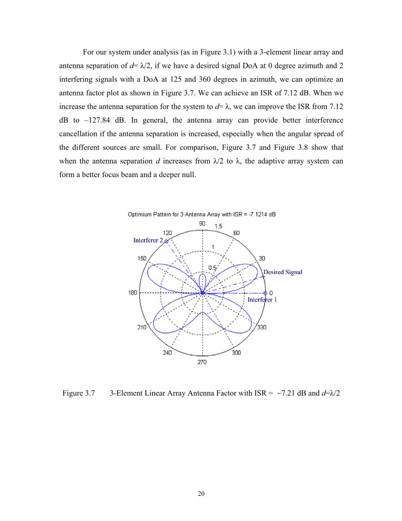
Figure 2.4 Block Diagram of an Adaptive Antenna System (from [5]).…..………. 10 Figure 3.1 Adaptive Antenna Array Systems..……………………………………. 13 Figure 3.2 4-Element Antenna Array Patterns...………………………………….. 15 Figure 3.3 A 2-Element Array.……………………………………………………. 17 Figure 3.4 Directional Pattern for d/λ=1/2.………………………………………… 18 Figure 3.5 Directional Pattern for d=λ.…………………………………………….. 19 Figure 3.6 Directional Pattern for d=2/λ.…………………………………………… 19 Figure 3.7 3-Element Linear Array Antenna Factor with ISR = −7.21 dB and

d=λ/2…………………………………………………………………… 20 Figure 3.8 3-Element Linear Array Antenna Factor with ISR = −127.84 dB and d

= λ……………………………………………………………………… 21 Figure 3.9 Symmetry Antenna Array Pattern……………………………………… 22 Figure 3.10 4-Element Linear Array Antenna Factor with ISR = −11.1 dB,

d=λ/2…………………………………………………………………… 23 Figure 3.11 4-Element Linear Array Antenna Factor with ISR = −47.8 dB, d=λ/2….

24 Figure 5.1 Area of Analysis within a Cell………………………………………… 35 Figure 5.2 Forward Channel Performance Boundaries for Our DS-CDMA System

with a 4-Element Linear Adaptive Array System (σdB=7, Rcc=1/2, v=8)……………………...………..………………....…………………. 36

Figure 5.3 BW Boundaries for a 4-Element Adaptive Array System (σdB =7,Rcc= ½, v=8)…..…………………………………………………….……….. 37

Figure 5.4 WB Performance Boundaries for our DS-CDMA System with a 2-Element Linear Adaptive Array System(σdB=7,Rcc=½,v=8)……...…... 38

Figure 5.5 WB Performance Boundaries for our DS-CDMA System with a 3-Element Linear Adaptive Array System(σdB =7,Rcc= ½, v=8)..………. 39

Figure 5.6 WB Performance Boundaries for our DS-CDMA System with a 4-Element Linear Adaptive Array System(σdB =7,Rcc= ½, v=8)……….. 39

Figure 5.7 Probability of Bit Error for DS-CDMA System with an SNR per Bit of 15 dB (σdB =7,Rcc= ½, v=8)…………………………………………... 41

Figure 5.8 Probability of Bit Error for a 2-Element Linear Adaptive Array DS-CDMA System Using Sectoring with a SNR per Bit of 15 dB (σdB =7,Rcc= ½, v=8)……………………………………………………….. 42

Figure 5.9 Probability of Bit Error for a 3-Element Linear Adaptive Array DS-CDMA System Using Sectoring with a SNR per Bit of 15 dB (σdB =7,Rcc= ½, v=8)……………………………………………………….. 42

x

Figure 5.10 Probability of Bit Error for a 2-Element Linear Adaptive Array DS-CDMA System Using Sectoring for σdB = 9 dB with a SNR per Bit of 15 dB (Rcc = 1/2 and v = 8)…………..……………………………….. 43

Figure 5.11 Probability of Bit Error for a 3-Element Linear Adaptive Array DS-CDMA System Using Sectoring for σdB = 9 dB with a SNR per Bit of 15 dB (Rcc = 1/2 and v = 8)…………...……………………………….. 44

Figure 5.12 Antenna Factor of the WW Case for a 4-Element Array Antenna with Path-Loss Ratio of 19.8476…………………………………………….. 45

Figure 5.13 Antenna Factor of the WW Case for a 4-Element Array Antenna at −1 Degree Offset with Path-Loss Ratio of 1.0877………..……………….. 46

Figure 5.14 Antenna Factor of the WW Case for a 4-Element Array Antenna with a Path-Loss Ratio of 185.6……..………….…………………………… 48

Figure 5.15 Antenna Factor of the WW Case for a 4-Element Array Antenna at +1 Degree Offset with a Path-Loss Ratio of 0.7950………..……………... 48

Figure 5.16 Antenna Factor of the WW Case for a 4-Element Array Antenna at −2 Degree Offset with a Path-Loss Ratio of 0.6293………..……….…….. 49

Figure 5.17 System Enhancement with +3 Degree of Orientation Offset at the Worst-Worst Case for a 2-Element Array (σdB =7,Rcc= ½, v=8).…….. 50

Figure 5.18 System Enhancement with -1 Degree of Orientation Offset at the Worst-Worst Case for a 3-Element Array (σdB =7,Rcc= ½, v=8).…….. 51

Figure 5.19 System Enhancement with +1 Degree of Orientation Offset at the Worst-Worst Case for a 4-Element Array (σdB =7,Rcc= ½, v=8)…...… 51

Figure 6.1 Wideband K-Element Array with a L-Tapped-Delay Line……...…….. 53 Figure 6.2 Transfer Functions of the Desired Signal (SBS) and Interference

Signal (IBS) of a 2-Element Array with a 2-Tapped-Delay Line System………………………………………………………………….. 56

Figure 6.3 Transfer Functions of the Desired Signal (SBS) and Interference Signal (IBS) of a 2-Element Array with a 3-Tapped-Delay Line System………………………………………………………………...... 56

Figure 6.4 Performance Comparison Using a 2-Element Array with a 2- and 3-Tapped-Delay Line for Broadband Signal (σdB =7,Rcc= ½, v=8)…....... 57

Figure 6.5 Transfer Functions of the Desired Signal (SBS) and Interference Signal (IBS) of a 3-Element Array with a 2-Tapped-Delay Line System………………………………………………………………….. 59

Figure 6.6 Transfer Function of the Desired Signal (SBS) and Interference Signal (IBS) of a 3-Element Array with a 3-Tapped-Delay Line System..…... 59

Figure 6.7 Performance Comparison using a 3-Element Array with a 2- and 3-Tapped-Delay Line for Broadband Signal (σdB =7,Rcc= ½, v=8)……... 60

xi

LIST OF TABLES

Table 5.1 3-Element Array Path-Loss Ratio Values for Different Orientation Offset at the WW Case………...………………………………………. 45

Table 5.2 Path-Loss Ratio Values of 2-, 3- and 4-Element Array with Different Orientation Offset at the WW Case……...…………………………..… 47

Table 5.3 Linear Array System Capacity Enhancement with ±5 Degree Freedom about the WW Case Position at BER 10-3 (σdB = 7 dB, Rcc = 1/2 and v = 8)……….…………………….…………………………………….. 50

xii

THIS PAGE INTENTIONALLY LEFT BLANK

xiii

ACKNOWLEDGMENTS

This thesis is dedicated to my family, especially my loving wife, Lian Choo, and

my adorable son, Ethan, both of whom endured my stress and absence during my

research here at the Naval Post graduate School. I am eternally indebted to them for their

love, understanding and unflagging support.

I also dedicate this thesis to my loving and supportive parents who taught me the

value of diligence, responsibility, and education.

I would like to express my sincere appreciation to my advisors, Professor Tri. Ha

and Professor Jovan Lebaric, and I would like to thank Ron Russell for his meticulous

editing of this thesis.

Last but not least, I must thank my sponsor Defence Science and Technology

Agency (DSTA) for providing the opportunity for me to pursue my work here in the

Naval Postgraduate School.

xiv

THIS PAGE INTENTIONALLY LEFT BLANK

xv

EXECUTIVE SUMMARY The third-generation (3G) cellular system employs Direct Sequence Code

Division Multiple Access (DS-CDMA) that allows simultaneous sharing of limited

available bandwidth. However, the DS-CDMA scheme limits the system’s capacity and

performance because it causes inter-cell co-channel interference and intra-cell

interference. In order to meet the growing demand of high data-rate services, various

techniques were explored to increase the system’s capacity.

This thesis analyses the performance of the base-station to the mobile channel

(forward channel) of a DS-CDMA system in a slow, flat Rayleigh fading and log-normal

shadowing environment. The forward channel is being studied because most data services

are asymmetric, with the downstream requiring a higher data rate. We explore the use of

an adaptive linear-array antenna at the mobile terminal to suppress the interferers. This is

achieved by steering an antenna null toward the interferer while forming an antenna beam

toward the desired signal continuously with time. This would minimize the Interference-

to-Signal Ratio, which improves the system’s performance and the system’s capacity.

Four performance boundaries of the DS-CDMA mobile communication system

with an adaptive array were established. The worst-case performance of the system was

compared with a DS-CDMA system without the smart antenna application. With the

Monte Carlo simulation, the results showed that the system’s capacity and performance

could be greatly improved with a smart antenna application. At BER of 10-3 or less, with

a 2-element or a 3-element linear array, an impressive capacity gain of 600% or 900%

can be achieved, respectively, in the worst-case scenario.

The thesis further explores the use of a wideband smart antenna (Tapped-Delay

Line) system. In the case of a 2-element and a 3-element linear array, we demonstrate

that 3- and 2-tap delay lines are sufficient to equalize and to compensate for the

frequency variation of a 4% bandwidth broadband signal.

xvi

The application of the smart antenna technology at the mobile terminal for the

third-generation DS-CDMA cellular system can be extended to the military mobile

communication systems. By doing so, the military mobile communication system will be

more robust since the mobile terminals are able to suppress possible interference by

steering the antenna null toward them. Similarly, the military mobile communication

system’s capacity and maximum data rates can also be improved using the smart antenna.

1

I INTRODUCTION

The third-generation (3G) cellular system employs a multiple-access technique

known as Direct Sequence Code Division Multiple Access (DS-CDMA. Simultaneous

multiple-user access in such a system provides efficient use of the limited bandwidth.

However, the DS-CDMA scheme used in the cellular system also creates problems in the

network, such as inter-cell co-channel interference and intra-cell interference. This thesis

analyzes the performance of the forward channel (base-station to mobile) of a DS-CDMA

system in a slow, flat Rayleigh fading and log-normal shadowing environment.

Generally, data services are symmetric, with the downstream requiring a high data rate.

The forward channel will be used to download data from sources, such as the Internet, at

a high data rate from the base-station to the mobile terminal.

With the ever-increasing demand to accommodate more users and higher data-rate

services within a limited available frequency spectrum, many researchers have explored

new options to improve the system’s capacity and performance. One of the most

promising techniques for increasing cellular system capacity is the use of smart antennas.

A mobile communication system often encounters co-channel interferers who occupy the

same channel as the desired user. This limits the system’s performance and capacity. The

most modern method of using dual diversity with Maximum Ratio Combining at the

receiver cannot reduce the high interference. This is true because the strategy of selecting

the strongest signal or extracting the maximum signal power from the antennas is not

appropriate. It will enhance the interferer signal rather than the desired signal. However,

if we could estimate the direction of arrival (DoA) of the interferers and the desired

signal, we could then use an adaptive antenna array to suppress the interference by

steering a null toward the interferer and forming a beam toward the desired signal

continuously with time. Therefore, the dynamic system performance can be improved.

Most of the performance analyses of the DS-CDMA cellular system have focused

on the reverse channel, such as in [6], even with the use of a smart antenna. However,

most of these performance analyses have only incorporated a subset of the channel

2

effects (fading and shadowing) and the benefits of forward error correction with soft

decision decoding.

In this thesis, we implemented an equally spaced linear antenna array with a

different number of elements at the mobile terminal. We analyzed the performance of a

randomly positioned mobile terminal with a randomly orientated adaptive antenna array

in a multi-cell DS-CDMA network and established four performance boundaries.

We select the tighter optimized array antenna boundary as our performance

reference, as it is more conservative and represents the worst-case situation. We then

combine the conservative optimized 2-, 3- and 4-element array antenna with the DS-

CDMA forward-channel received signal model developed in [4]. The model in [4], which

originally incorporated both log-normal shadowing and Rayleigh slow flat fading, now

includes the effect of the smart antenna. We further combined the benefit of forward error

correction with soft decision decoding to obtain the new system model. Finally we

compared the capacity and performance of different cellular systems under a range of

shadowing conditions, with and without antenna sectoring at the base-station and for

various user capacities using a Monte Carlo simulation.

All the previous analyses assumed that the system is a narrowband system. In [6]

the smart-antenna analysis was assumed to have an ideal wideband antenna. The presence

of a single, complex, adaptive weight in each element channel of an adaptive array is

sufficient for processing narrowband signals. However, processing broadband signals,

such as the forward channel of a 3G DS-CDMA network, requires that a tapped-delay

line (transversal filter) processing be employed in each element channel. In a practical

implementation, each channel is slightly different electrically. It will lead to channel

mismatching, which could significantly alter the frequency response characteristics from

channel to channel. This may severely degrade the antenna array performance. The

tapped-delay line permits frequency-dependent amplitude and phase adjustments to be

made, to equalize the frequency-varying effect on the antenna when receiving a

3

broadband signal. We also analyzed the performance of a DS-CDMA cellular system

with mobile terminal equipped with a linear array and tapped-delay line.

Now, there is a trend to adopt commercial off-the-shelves products for military

applications because this approach can be more cost effective. With slight modification

of the commercial mobile communication system, the modified system can be deployed

for military applications. Hence the performance analysis in the application of the smart

antenna technology at the mobile terminal for the third-generation DS-CDMA cellular

system can be valuable for military use.

In Chapter II, we will discuss the co-channel interference of a DS-CDMA system

and various methods to minimize the interference problem. And in Chapter III, we will

introduce the characteristics and constraints of an equally spaced linear adaptive array

system. This adaptive array will be used in our DS-CDMA system for analyzes. The

forward channel propagation model for DS-CDMA system will be introduced in Chapter

IV. Chapters V and VI discuss the performance of an adaptive antenna system in a

narrow-band and a wide-band DS-CDMA forward channel respectively.

4

THIS PAGE INTENTIONALLY LEFT BLANK

5

II SMART ANTENNA APPLICATION IN MOBILE

COMMUNICATION

In this chapter, we will discuss the main constraint of a DS-CDMA mobile

communication system and different methods to improve the system capacity and

performance. The main constraint of the DS-CDMA network is the co-channel

interference. Application of cell sectoring and smart antenna are the common methods

used to combat the co-channel interference.

A. CO-CHANNEL INTERFERENCE

In the CDMA cellular mobile communication network in which the radio-

frequency spectrum is shared, the multipath signal fading environment and the multiple

co-channel interferers limits the system’s performance. With the co-channel interference

as the major limiting factor for performance [7], the CDMA based network is hence an

interference-limited system. Consequently in order to improve the system’s performance

and capacity, minimizing the system interference would be most effective. However,

unlike thermal noise, which can be overcome by increasing the signal power, co-channel

interference cannot be overcome by increasing the signal power. Doing so increases

interference to the neighboring co-channel cells.

In a multi-cell cluster, such as a TDMA IS-54/GSM system, interference can be

suppressed by increasing the physical separation of co-channel cells until a sufficient

isolation is achieved due to the propagation loss. This can be achieved by increasing the

cluster size N. The Signal-to-Interference (SIR) Ratio, is defined in [7] as

SIR = ( )3

n

o

N

i (2.1)

where io is the number of interferer and n is the path loss exponent.

6

However in the case of a CDMA network in which the whole frequency spectrum

is shared and reused by all first-tier neighboring cells, the distance between the base-

station to any co-channel base-station is fixed at 3 R where R is the radius of the

hexagonal cell (Figure 2.1). Thus in the single-cell CDMA network, we do not have the

freedom to vary the cluster size N to reduce the co-channel interference.

1

2

35

4

6

BS

3R3R

R

Figure 2.1 Geometry of a Cellular CDMA Mobile Communication Network

Another method to reduce the co-channel interference must be explored in order

to improve the system performance. Two common methods to combat the co-channel

interference are by sectoring and by using smart antenna technology.

B. SECTORING

The co-channel interference in a cellular mobile communication system can be

reduced by replacing the omni-directional antenna at the base-station with several

directional antennas. The use of a directional antenna limits the number co-channel

interferers seen by any receiver within the cell. This is true because each directional

antenna only radiates within a desired sector. This technique is called sectoring. The scale

of the reduction of co-channel interference depends on the number of sectors used. A cell

is commonly partitioned into three 120-degree or six 60-degree sectors, as shown in

7

Figure 2.2. In the case with users evenly distributed within all cells, the amount of co-

channel interference is reduced to 1/3 or 1/6 of the omni-directional value if 120-degree

or 60-degree sectoring is used respectively.

BS BS

60

120

12060

60

Figure 2.2 60 and 120 Cell Sectoring

Many papers such as [4], which evaluated the forward channel performance in the

fading environment, evaluate and present the improved performance with the use of 6 and

3 sectors of 60 and 120 sectors, respectively, in a DS-CDMA cellular system operating

in a channel with Rayleigh fading and log-normal shadowing.

Figure 2.3 Probability of Bit Error for DS-CDMA Using Sectoring ( dBσ = 7) with an

SNR per Bit of 15 dB with Rate 1/2 Convolution Encoder with v=8. (From:[4])

8

C. SMART ANTENNA

A smart antenna system, which is an antenna array arranged in a certain

distributed configuration with a specialized signal processor, can be deployed in the

CDMA mobile communication system to improve the system’s performance and capacity

significantly by minimizing undesired co-channel interference. Most of the smart antenna

systems can form beams directed to a desired signal and form nulls toward undesired

interferer such as a co-channel base-station. This will enhance the signal-to-interference

(SIR) ratio because the received desired signal strength is maximized and the undesired

interference is minimized. Other benefits of a smart antenna include:

• increase in range or coverage arising from an increased signal strength due to

array gain,

• increase capacity arising in interference rejection,

• reject multi-path interference arising from inherent spatial diversity of the

array,

• reducing expense arising from lower transmission powers to the intended user

only.

A smart antenna system is commonly classified into three categories: switched

beam antennas, dynamic phased arrays and adaptive antennas. Although a multiple

antenna system is also commonly used at the receiver for L-fold diversity, which could

mitigate the harmful effects of fading by reducing the signal fluctuations when the signal

is sufficiently de-correlated, the multiple antennas cannot distinguish a co-channel signal.

This method of extracting the maximum signal power from the antennas is not

appropriate because it also enhances the co-channel interference together with the desired

signal.

A switched-beam antenna system consists of many highly directive, pre-defined

fixed beams formed with an antenna array. The system usually detects the maximum

received signal strength from the antenna beams and chooses to transmit the output signal

from one of the selected beams that gives the best performance. In some sense, a

9

switched beam antenna system is very much like an extension of a sectoring directional

antenna with multiple sub-sectors. Since the direction of the arrival information of the

desired signal is not explored, the desired signal may not fall onto the maximum of the

chosen beam because these beams are fixed. Hence switched beam antennas may not

provide the optimum SIR. In fact, in cases where a strong interfering signal is at or near

the center of the chosen beam, while the desired user is away from the center of the

chosen beam, the interfering signal can be enhanced far more than the desired signal,

which results in very poor SIR.

Dynamic phased arrays use the direction of arrival (DoA) information from the

desired signal and steer a beam maximum toward the desired signal direction. This

method when compared to switch-beam antenna, is far more superior in performance

because it tracks the desired user DoA continuously, using a tracking algorithm to steer

the beam toward the desired user. The tracking of the DoA enables the system to offer

optimal gain for the desired signal, while simultaneously minimizing the reception of the

interfering signal by directing the nulls to the interferer’s direction. Thus excellent SIR

can be achieved.

In the adaptive array, the weights are continuously adjusted to maximize the

signal-to-interference-plus-noise ratio (SINR) and to provide the maximum

discrimination against undesired interfering signals. If the interferer is absent and if only

noise is present, the adaptive antennas maximize the signal-to-noise ratio (SNR) and thus

behave as a Maximal Ratio Combiner (MRC). With the use of various signal-processing

algorithms at the receiver-adaptive antenna array system, this system can distinguish

between the desired signal and the interfering signals, and can then calculate their

direction of arrival continuously. This is done to minimize interference dynamically by

steering the nulls patterns toward these undesired sources and to form the maximum gain

pattern toward desired signal. Such algorithms are usually implemented by digital signal

processing software, which is relatively easy to implement and to enhance. By using

other algorithms for branch diversity techniques, the adaptive antenna array system can

process and can resolve separate multi-path signals, which can be combined with the

10

adaptive antenna system to maximize the SINR or SIR.

Figure 2.4 Block Diagram of an Adaptive Antenna System (from [5]).

An adaptive antenna array system may consist of N number of spatially

distributed antennas with an adaptive signal processor that generates the weight vectors

for optimum combining of the antenna array output. This can also be regarded as an N-

branch diversity scheme, providing more than the two diversity branches commonly

used. The received RF signals from the N-antenna elements are coherently down-

converted to a baseband/IF frequency, sufficiently low so that the adaptive array

processor can effectively digitalize the signals. The processor processes each digitized

input channel by multiplying the adjusted complex weights of each branch to form the

beam and the nulls. This results in the beam and null steering, which can be viewed as a

spatial filter having a pass and stop band created for the direction of the desired signal

and interference respectively. In general, with N-antenna elements in the adaptive array

system, generating (N-1) nulls in the array system radiation pattern toward (N-1)

interferer directions is possible. This will reduce the total interferer signal significantly,

thus reducing the interferer-to-signal ratio. By reducing the interference in the

interference limited system, performance and capacity can be improved.

11

D. ADAPTIVE ANTENNA ARRAYS APPLICATION IN THE

FORWARD CHANNEL

Unlike the base-station, where the physical space is the lesser of a constraint,

implementing a larger number of antenna elements with a large signal processor is

possible. However the mobile units do not have the luxury of the physical space of the

base-station. In today’s design of a mobile unit, reducing the physical size and weight is

always a prime consideration. Implementing a large number of antenna elements on the

mobile unit is not possible. In this thesis, we focus on the performance analysis with the

use of adaptive 2-, 3- and 4-element linear array system at the mobile user in the forward

channel, because they are likely to fit into a mobile terminal in a future communication

system.

For a 4-element (N=4) linear array system at the mobile in a CDMA mobile

communication network, the adaptive array processor at the mobile could form a beam

toward the desired base-station and up to 3 nulls toward the 3 co-channel interferer (first-

tier base-station). Such an adaptive antenna system usually performs null steering first,

which minimizes the signal-to-interference ratio (SINR) by suppressing as many

interferers as possible so that the desired signal is least distorted. Then the system will

use the remaining degrees of freedom to steer the desired beam toward the desired signal

direction of arrival to maximize the signal-to-noise ratio (SNR). With this strategy, the

system can improve the SINR for the mobile user maximally.

In this chapter, we have illustrated needs to combat the co-channel interference of

a DS-CDMA mobile communication system. With the application of the smart antenna,

we could maximize the SINR of the system. In the next chapter, we will discuss the

characteristics and constraints of an equally spaced linear adaptive array for our

application.

12

THIS PAGE INTENTIONALLY LEFT BLANK

13

III LINEAR ADAPTIVE ANTENNA ARRAY

As mentioned in the last chapter, a smart antenna system such as an adaptive

antenna array can be applied to a CDMA mobile communication system to maximize the

SINR of the system. This is accomplished by maximizing the suppression of the

interferers with null steering, and maximizing the SNR by beam steering toward the

desired signal. The elements of the adaptive antenna array can be arranged in different

configurations such as circular, linear equally spaced, triangular etc. This chapter presents

an equally spaced linear adaptive array system.

Desired Signal

Interferer 1

Interferer L

W1

W2

WN

.

.

.

.

∑0

1 T

T ∫

t=T

N-elementArray

SIGNALPROCESSOR

CONTROLALGORITHM

X1(t)

X2(t)

XN(t)

y(t)

Figure 3.1 Adaptive Antenna Array Systems

Figure 3.1 shows an adaptive antenna array having N elements with L interferers.

Let xk(t) be the received signal at the k-th antenna element output.

xk(t)= ks (t) + nk(t) , k= 1, 2, 3, …. N (3.1)

where ks (t) is the complex signal envelope of the signal and nk(t) is the noise

14

received by the k-th antenna element. Letting λ be the wavelength, d be the

element spacing, and θ be the incident angle with respect to bore sight, we have

= 2π (k-1)d

λi sinθks (t) s(t) e k= 1, 2, …, N (3.2)

The array output signal y(t) is the weighted sum of all xk(t).

.

∑N

T Tk k

k=1

1 1

2 2

N N

(t)= w x (t)= W X = X W .

w x (t)w x (t)

W = . , X = .. .w x (t)

y

(3.3)

The adaptive array system continuously adjusts the weights vector W by

the optimum control algorithm with criterion such as Minimum Mean Square

Error (MMSE) [5].

A. OPTIMAL WEIGHTS

In this thesis we intend to minimize the ISR as our algorithm to compute

the optimal weight for the adaptive antenna system. We assume a linear array

with 2-, 3- or 4-elements and with element spacing d. To illustrate, we use the

case of a 4-element array. The amplitudes are A1, A2, A3 and A4, and the phases

are ψ1 and ψ2, ψ3 and ψ4. The far-field antenna factor Farray is calculated to be

in the horizontal plane, hence the angle φ denotes the azimuth direction (the angle

of azimuth).

31 2 4

2 32 sin 2 sin 2 sin

1 2 3 4 .d d di i iii i i

arrayF A e A e e A e e A e eπ φ π φ π φψψ ψ ψλ λ λ

− − −= + + + (3.4)

15

Let the operating frequency be 2 GHz and the antenna element spacing d of λ/2,

we then normalize the total power (gain) to be equal to 1 by using a relationship of A12 +

A22 + A32 + A42= 1. We can generate any far field antenna factor in any of the 360-

degree azimuth. Figure 3.2 shows the antenna factors of a 4-element antenna array with

various phase shifts. We can see that the antenna factor changes significantly over 180

degrees phase shift.

0

30

6090

120

150

180

210

240

270

300

330

2

1

0

0 phase shift45 degree phase shift 90 degree phase shift135 degree phase shit180 degree phase shift

Figure 3.2 4-Element Antenna Array Patterns

The directions of arrival (DoA) of the desired signal bφ (base-station) and the

interference signals ( 1 2 3, ,i i iφ φ φ ) can be estimated. With these DoA estimated, if we take

the desired base-station signal as a reference, the complex gains of the array in the

16

direction of the desired signal barrayF , the three interferers (

1 2 3,

i i iarray array arrayF F F ) and ISR

can be defined as:

31 2

2 32 sin 2 sin 2 sin

1 2 3 4 .b b b

b

d d di i iii iarrayF A A e e A e e A e e

π φ π φ π φψψ ψλ λ λ− − −

= + + + (3.5)

1 1 131 2

1

2 32 sin 2 sin 2 sin

1 2 3 4 .i i i

i

d d di i iii iarrayF A A e e A e e A e e

π φ π φ π φψψ ψλ λ λ− − −

= + + + (3.6)

2 2 231 2

2

2 32 sin 2 sin 2 sin

1 2 3 4 .i i i

i

d d di i iii iarrayF A A e e A e e A e e

π φ π φ π φψψ ψλ λ λ− − −

= + + + (3.7)

3 3 331 2

3

2 32 sin 2 sin 2 sin

1 2 3 4 .i i i

i

d d di i iii iarrayF A A e e A e e A e e

π φ π φ π φψψ ψλ λ λ− − −

= + + + (3.8)

2 2 24 1 2 3 .A A A A= + + (3.9)

1 2 3

2 2 2

.i i i

b

array array array

array

F F FISR

F

+ += (3.10)

In order to optimize the complex weights that include both amplitude and phase

values and to minimize the interference, we performed constraint minimization of the

ISR by using minimization functions available from software tools such as MATLAB or

MATHCAD. These minimization functions allow one to search for optimized solutions

for a non-linear function with some guessing of the initial values. To ensure that the

weights amplitude conform to our normalization of gain power, we place a constraint of

0<A1,A2,A3<1.

In the case of the 4-element array, there would be 6 unknown variables

(A1,A2,A3, ψ1, ψ2, ψ3) to be optimized, which effectively performs the null steering for

the interferers. The most optimum strategy is to steer the null toward the interferer first

rather than trying to maximize the gain of the desired signal beam.

17

With the optimum weight values obtained after minimizing the ISR, these weights

are back-substituted into Equations (3.5) and (3.6) to compute the optimum ISR (ISRopt)

and to obtain the antenna factor values for all directions.

B. LINEAR ARRAY CONSTRAINTS

1. Angular Spread and Null Depth

X(t)Array

Normal

d

W1 W2

d sin Φ

Φ

ArrayOutput

Figure 3.3 A 2-Element Array

18

To illustrate the angular spread problem of a linear array, we make use of a 2-

element array as shown in Figure 3.3 with W1 and W2 =1 for simplicity and let the left

element output be x1(t) = x(t) as a reference, the output of the array

2

i=1= .

2πdj(i-1) sin λ

1 2y(t)= x (t)+ x (t) x(t)eφ

∑ (3.11)

The directional antenna pattern G( )φ can be defined as

[dB]φφ2A( )G( ) = 10 log

2 (3.12)

where 2

i=1= .

j(i-1)2π d sin( )λA( ) e

φ

φ ∑ (3.13)

If we take antenna separation of d = λ/2, d = λ and d = 2λ, we can plot the directional

pattern φG( ) versus φ as Figures 3.4 through 3.6.

Figure 3.4 Directional Pattern for d/λ=1/2

Φ

G ( )φ

φ

19

50 0 5040

30

20

10

0

Figure 3.5 Directional Pattern for d=λ

50 0 5040

30

20

10

0

Figure 3.6 Directional Pattern for d=2λ

If the angular spread between the desired signal and the interferer is small, the

antenna array may not be able to discriminate the interferer signal with deep nulls unless

the antenna separation is increased.

G( )φ

φ

φ

G( )φ

20

For our system under analysis (as in Figure 3.1) with a 3-element linear array and

antenna separation of d= λ/2, if we have a desired signal DoA at 0 degree azimuth and 2

interfering signals with a DoA at 125 and 360 degrees in azimuth, we can optimize an

antenna factor plot as shown in Figure 3.7. We can achieve an ISR of 7.12 dB. When we

increase the antenna separation for the system to d= λ, we can improve the ISR from 7.12

dB to –127.84 dB. In general, the antenna array can provide better interference

cancellation if the antenna separation is increased, especially when the angular spread of

the different sources are small. For comparison, Figure 3.7 and Figure 3.8 show that

when the antenna separation d increases from λ/2 to λ, the adaptive array system can

form a better focus beam and a deeper null.

Figure 3.7 3-Element Linear Array Antenna Factor with ISR = −7.21 dB and d=λ/2

21

Figure 3.8 3-Element Linear Array Antenna Factor with ISR = −127.84 dB and d = λ

However, in our scenario as a mobile user, increasing the antenna separation is

impossible in practice, because of the very limited real estate for the antenna site. For a

mobile terminal such as a laptop PC, we can fit up to a 4-element linear array in about 30

cm, the width of a typical laptop, with a antenna separation of d=λ/2 when we operate in

the frequency spectrum of 2 GHz. Doing this is impossible if we increase the antenna

separation to d= λ, which requires a width of more than 30 cm in practice.

22

2. Symmetry

Figure 3.9 Symmetry Antenna Array Pattern

Figure 3.9 shows that the antenna pattern is always symmetrical on two sides

from about 90 to 270 degrees axis. If the DoA of the desired signal and the interferer fall

on the opposite side, both antenna factor and gain will be the same. In a worst-case

situation in which the interferers are located in this symmetrical location and if the

interferers are equal distance or equal signal power to the mobile as the SBS signal, the

ISR will be close to zero which is not optimum. This situation occurs though it may be

rare. It can be overcome if we allow the mobile to change the array orientation by some

small value, which may improve the system’s performance significantly.

23

3. Orientation Limited

Figures 3.10 and 3.11 illustrated that the linear array performance is orientation

limited. Although the relative angular spread between the desired base-station and other

interfering sources are the same, the performance of the ISR can be significantly different

in both cases. This problem may be solved if the antenna array is rotated on the mobile

for optimum performance.

0

30

60

90

120

150

180

210

240

270

300

330

2

1.5

1

0.5

0

Optimum Antenna PatternSignal DoAInterferer 1 DoAInterferer 2 DoAInterferer 3 DoA

Figure 3.10 4-Element Linear Array Antenna Factor with ISR = −11.1 dB, d=λ/2

24

0

30

60

90

120

150

180

210

240

270

300

330

2

1.5

1

0.5

0

Optimum Antenna PatternSignal DoAInterferer 1 DoAInterferer 2 DoAInterferer 3 DoA

Figure 3.11 4-Element Linear Array Antenna Factor with ISR = −47.8 dB, d=λ/2

With the optimum complex weights determined for the adaptive antenna system,

we noted that the depth of the null steer for suppressing interference depends on the

geometry scenarios between the angular spread of the desired signal and interferers’

DoA, the antenna-array arrangement and separation, and the geometric orientation

between the array and all the other sources. All these factors contribute to the complexity

of the operating environment to ensure a minimum system performance

We have discussed characteristics and constraints of an equally spaced adaptive

array in this chapter. The orientation dependent linear array increases the complexity to

ensure a minimum performance level within the cell. In the next chapter, we will discuss

the forward channel model of the DS-CDMA system. This channel model will be used

with the linear antenna array discussed for our performance analysis in Chapter V.

25

IV FORWARD CHANNEL PROPAGATION MODEL FOR CDMA SYSTEM

The forward channel propagation model of a DS-CDMA mobile communication

system in a slow, flat Rayleigh fading and log-normal shadowing environment is

presented in this chapter. The forward channel is being studied because most data

services are asymmetric, with the downstream requiring a higher data rate.

A. MEDIUM PATH LOSS

In practice the mobile user can be located anywhere within the cell, with two

degrees of freedom because its position can be at R distance from its base-station and can

be at a particular angle to the base-station. Unlike an omni-directional antenna, the linear

antenna array has an orientation, which must be considered. This directional effect of the

linear antenna array increases the definition of the mobile position within the cell to a

third-order problem since the mobile can be randomly orientated in any direction.

In order to account for co-channel interference, both the distances from the

mobile to all 6 first-tier co-channel base-stations and their relative antenna array to base-

station angle must be estimated.

We defined the distance from the base-station in the center cell to the mobile user

as R, while the distance from the mobile user to the 1st tier co-channel base-station as Di

with the cell radius as D. The angle of the mobile from the base-station is A.

With the 6 first-tier hexagonal cells geometry fixed as their center base-station,

we could determine all 7 angles and distances from the mobile to all the 7 base-stations

when we define any position (R, A) in the center cell as a phasor representation of MS =

R ejA where ( 0 < R < 1 ) and ( 0 < A < 2π ).

26

The distance Di and the direction of arrival of the co-channel i-th base-station

(BS) θi can be determined by using vector algebra.

With a normalized cell radius of D = 1, the distance between the center of each

adjacent base-station is 3 and the angle from the center origin to each adjacent base-

station, θBSi,, is at (0, π /3, 2π /3, π , 4 π /3, 5 π /3, 2 π ) radians, we could determine all

the look angles and the distances from the mobile-station to all adjacent base-stations.

Di = Re| 3 j BSie θ - R ejA. | (4.1)

θBSi = (0, π /3, 2π /3, π , 4 π /3, 5 π /3, 2 π ) (4.2)

θi = ∠ ( 3 j BSie θ - R ejA. ) (4.3)

The azimuth and distance toward the desired center base-station is θBS = π + A (4.4)

DBS = R . (4.5)

These distances and angles are used to calculate the path loss for the desired

signal and co-channel interference using the Hata model, which is equivalent to an

average path loss Ln (D) [7] with a path loss exponent of n=4.

Ln(D)

∝

n

o

Dd

where do is the reference distance. (4.6)

1. Hata Model

The Hata model is one of the simplest and most accurate empirical models for

representing path loss of cellular systems as presented in [7]. It is based on Okumura

model’s graphical path loss data [1] using a standard formula for an urban operating area

and other areas with modified equations. The original Hata model matches the Okumura

27

model closely for distances greater than 1 km, and the extended model [2] further extends

to cover higher frequency ranges with distances of about 1 km. In this thesis, we use the

extended model as it better represents the operating environment of a 3G cellular system.

The extended Hata model, which predict the median path loss LH in dB as defined in [7]

by

LH = 46.3 + 33.9 log fc – 13.92 log hbase – a(hmobile) (4.7)

+ (44.9 – 6.55 log hbase) log d + CM

where

a(hmobile) = (1.1 log fc – 0.7) hmobile – (1.56 log fc ) (dB) (4.8)

and

CM = 0 dB, for medium sized city and suburban areas3 dB, for metropolitan areas.

Note that

fc : carrier frequency in MHz,

hbase : base-station antenna height in meters (m),

hmobile : mobile-station antenna height in meters (m), and

d : separation distance is measured in kilometers (km).

The extended Hata model is restricted to the following range of parameters:

fc : 1500 MHz to 2000 MHz

hbase : 30 m to 200 m

hmobile : 1 m to 10 m

28

d : 1 km to 20 km

We chose the mobile and base-station heights of 1 m and 30 m respectively with

an operating carrier frequency of 2000 MHz for all our research.

2. Log-normal Shadowing

Log-normal shadowing accounts for variation in the average large-scale

propagation fading for a given distance. The actual path loss for a mobile user in different

locations but with the same distance from the base-station varies due to the medium. This

happens because the terrain variations in a particular path can be significantly different

from the predicted average path loss. A Gaussian random variable X with zero-mean and

σdB standard deviation can be used to represent the shadowing of the average path loss

value. The path loss with shadowing accounted for is modeled by

LX (D) = LH (d) + X (dB) (4.9)

where

LH (D) is the average path loss at distance D km.

The above equation can be converted to a log-normal random variable LX as

defined in [4]

LX = LH X. (4.10)

The above log-normal random variable LX in (4.10), which accounts for the effect

of log-normal shadowing with the Hata model, can then be applied to the signal in the

forward channel of the DS-CDMA cellular system in a Rayleigh slow-flat fading

environment.

29

B. FORWARD CHANNEL MODEL

In [4], the above both large-scale and small-scale propagation effects are

combined into a single model. This combined Rayleigh-log-normal channel fading model

allows us to characterize the mobile radio channel accurately in a single unified model, in

which we can more completely analyze the mobile radio channel.

The Rayleigh-log-normal channel model is then applied to a typical DS-CDMA

cellular system consisting of traffic from a cell’s base-station to the mobile users in the

cell, which characterize the received signal of a mobile user. This received signal

includes both traffic intended for the mobile user from the Signal Base-Station (SBS),

traffic from other users in the cell (intra-cell interference), traffic for users in adjacent

cells (inter-cell interference) and additive white noise. The Signal-to-Noise plus

Interference Ratio (SNIR) and Bit Error Rate (BER) for the DS-CDMA forward channel

in the Rayleigh-lognormal fading channel were derived in [4].

Using the Forward Error Correction (FEC) the upper bound bit error probability

eΡ is defined in [4]:

21 ( )

free

e dd d

P dk

Ρ β∞

=

≤ ∑ . (4.11)

∞

−∞= ∫ d

d2 z d d

zP (d) Q P (z )dz

α( ) . (4.12)

2 2( ) 162

1 0

( )3 ( ) 2

λ σ

α−

= =

= +∑∑dB

iKoH

i j H i c

NL DeN L D E

. (from [4] equation (4.60)) (4.13)

= bc

kEEn

is the coded bit energy. (4.14)

30

ln1010

λ = . (4.15)

where P2(d) is the first-event error probability of the random variable Zd, which is the

sum of d multiplicative chi-square (with 2 degrees of freedom) log-normal random

variables. The details of the derivation and modeling of Zd are elaborated in [4]. dβ is

the total number of information bit errors that is associated with selecting a path of

distance d from the all-zero path, which can be calculated for a particular convolutional

code. dBσ is the log-normal shadowing random variable standard deviation in decibels

(dB).

However, when we incorporate the use of smart antenna in our case, the above

model must be modified to take into consideration the antenna gain factors for all 6 co-

channel interference base-stations (IBS). Hence our modified α becomes

2 2

162'

1 0

( )( )

3 ( ) 2

λ σ

α−

= =

= +∑∑dB

iKi oH

i j H i c

G NL DeN L D g E

. (4.16)

where Gi and g is the antenna gain factor for IBSi and Signal Base-Station (SBS),

respectively.

We required optimization of the linear antenna array over a 360-degree

orientation for any mobile user positions within the center cell of a 7-cell cluster. Since

the path loss from the various mobile positions to the different IBSs, the SBS and the

respective directions are different and we must derive an antenna-array optimization

constraint, which accounts for all the above possible variations. Simple optimization

using antenna factor interferer-signal-ratio (ISR) may not be appropriate because it did

not account for the different path loss values for the different interferers.

31

For simplicity, we assume all first-tier cells around the SBS’s center cell have the

same number of active users in each cell. We define the Path Loss Ratio (PLR) as the

optimization factor for determining if the particular orientation of a particular position is

the best or the worst in performance.

6

iH

i=1 H i

GL (D)PLR

L (D ) g=∑ . (4.17)

Note that 'α is proportional to PLR, where the former is the denominator in the Q

function of the first-event probability P2(d) in Equation (4.12). Thus, if PLR is smaller,

P2(d) will be smaller and since the probability of error Pe is also proportional to P2(d), as

defined in Equation (4.11), if P2(d) is smaller, Pe will show better performance.

Now we are ready to establish performance boundaries based on the PLR values

after the antenna array optimization. Due to the complexity of the above channel model,

we could not reasonably develop any analytical solutions. Instead a Monte Carlo

simulation was used to obtain the solutions for our performance analysis in Chapter V.

32

THIS PAGE INTENTIONALLY LEFT BLANK

33

V PERFORMANCE ANALYSIS OF ADAPTIVE ANTENNA

SYSTEM

In this chapter, we assess the performance on the forward channel with equally

spaced linear smart antenna arrays at the mobile user within the cell. Analyzing the

forward channel with an adaptive array is complex, as the channel is wireless, the

position of the user is mobile, and the orientation of the array is random. As discussed in

Chapter IV, we use the DS-CDMA forward channel model developed in [4], for a

received signal at the mobile user in a Rayleigh-lognormal channel. The BER

performance with different linear arrays was statistically simulated due to the complexity

of our channel model as no analytical solutions can be reasonably developed. Since

thousands of possible locations can exist within the cell, and since each position can have

random orientations that affect the linear antenna array ISR, evaluating the overall system

BER performance can be extremely computational expensive. Obtaining a good

representation of the result is also difficult because the BER performance at each location

may deviate significantly with a different orientation. Also the adaptive linear array may

encounter constraints, so it cannot effectively cancel the interferers, such as in the

situation mentioned in Chapter III where an interferer and desired signal are located in

the mirror symmetry position at an equal distance. We have adopted a 4-boundary

approach to better represent the adaptive-array system performance for our evaluation

and provide comparison with a system without using the smart antenna.

Initially, we analyze the performance boundary for a 2-, 3- and 4-element linear

array by positioning the Mobile Station (MS) randomly within the cell, with the MS

being rotated 360 degrees at each location. We perform the adaptive array optimization

for each random MS position at each orientation, with 1-degree resolution for the whole

360-degree orientation. For each of the optimized weights obtained for each 1-degree

orientation, we use the optimized weights to compute the antenna gain for all the 7

antenna-array factors, to determine the path loss ratio as defined in Chapter IV. We repeat

the process for 360 degrees. We then select the best and worst path-loss ratio that

correspond to the best and worst system performance for that single location.

34

We also repeat the whole optimization process to capture the best and the worst

performance by positioning the MS around the boundary of the cell within a 60-degree

sector, assuming the furthest distance from the signal BS has a normalized radius of 1 km

and the nearest distance of 0.1 km. We also confine the random position to fall within

the 60-degree sector, as the hexagonal cell is symmetrical in all such 60-degree sectors

and the performance analysis on one of the 60-degree sectors could apply to all the cells

without losing any generality.

We then sort each lot of the path-loss ratios by determining the largest and

smallest path-loss ratio values to obtain 4 path-loss ratio values. These 4 path-loss ratio

values are used to perform the Monte Carlo simulation on Equation (4.11) to obtain BER

performance boundaries for the DS-CDMA mobile communication system forward

channels of the mobile user with adaptive linear array with different operating scenarios.

The 4 boundaries are defined as:

1. Best of Best BER boundary (BB)

2. Worst of Best BER boundary (WB)

3. Worst of Worst BER boundary (WW)

4. Best of Worst BER boundary (BW)

35

IBS1

IBS2

IBS3IBS5

IBS4

IBS6

SBS

Figure 5.1 Area of Analysis within a Cell

Without losing generality, we can take the sector, as indicated in Figure 5.1, as the

area for analysis since all other sectors are symmetry. The system performance analyzed

for the selected sector is applicable to other sectors within the same cell. We can see that

of the 4 boundaries illustrated in Figure 5.2, the WW boundary, being far above the chart

of BER=10−1, is not visible. The Best of the Best (BB) boundary, representing the very

best performance, is the performance ceiling of the system as it cancels the dominant co-

channel interference extremely well. The location of this point is at the nearest point

within 10% of the normalized radius. For the 2-element array, the BB is at the azimuth

along the line between the SBS and the IBS. This is not surprising since the nearest IBS 1

interference is being attenuated by the null, which the adaptive-array system steers. In the

case of the 3- and 4-element array, the BB point is at 120 degrees and 90 degrees with

10% of the normalized radius. This indicates that all the nearest IBS co-channel

interferences are effectively cancelled. We can also look at this performance bound as

the achievable performance for a linear array is given 360 degrees of freedom.

36

0 5 10 15 20 25 30 3510-6

10-5

10-4

10-3

10-2

10-1

100

SNR per bit (dB)

Pe

Best of Best CaseWorst of Best CaseWorst of Worst CaseBest of Worst Case

Figure 5.2 Forward Channel Performance Boundaries for Our DS-CDMA System

with a 4-Element Linear Adaptive Array System (σdB=7, Rcc=1/2, v=8)

The Worst of the Worst (WW) case is a very pessimistic scenario in which the

interferer is not being suppressed or perhaps is being amplified by the adaptive array. The

constraints of the linear array, such as the symmetry of IBS and SBS locations or a poor

initial guess for minimizing the ISR ratio etc. might cause this. The performance of this

case is always above the usable limit of the BER of 10−2. The location of this case is near

the edge of the cell adjacent to the other co-channel IBS cell. For 2- and 4-element arrays,

the WW point is near the cell corner, adjacent to the two other IBS cells whereas for the

3-element array, the WW point is located at the mid-point between the SBS and IBS

lines. This boundary is not usable to represent the performance of the system reasonably.

We shall review the WW case in a later section, which indicates that the WW case indeed

is not as pessimistic as it appears, especially if we have some degree of freedom to adjust

or to rotate the antenna array. This bound can also be viewed as the worst performance

boundary if the linear array of the mobile unit is fixed in its orientation. This may not be

the case in a field system.

37

The Best of the Worst (BW) boundary is generally very much like the BB case

that is usually close to the ceiling performance boundary. The best result of any scenario

is located closest to the 10% radius of the SBS where the low path loss for the desired

signal dominates the interference signals generated by other IBS. The BER performance

for all scenarios for the BW case thus falls very close to the BB boundary, as in both

cases, the co-channel interferences are very effectively cancelled.

0 5 10 15 20 25 30 3510-6

10-5

10-4

10-3

10-2

10-1

100

SNR per bit (dB)

Pe

Users/cell=10Users/cell=20Users/cell=40Users/cell=60Users/cell=80Users/cell=100Users/cell=120Users/cell=140Users/cell=160

Figure 5.3 BW Boundaries for a 4-Element Adaptive Array System(σdB=7, Rcc= ½,

v=8)

The most representative boundary is the Worst of Best (WB) case as it indicates

system performance that is neither too pessimistic nor too optimistic. As in the usual

design of a mobile communication system in which we are interested in the minimum

assured performance, the WB boundary provides that minimum boundary. This WB

boundary indicates the worst case (the lowest limit) of the best performance achievable

by our system with a linear array with 360 degrees of freedom. The location of the WB

cases is at hexagon cell corner for a 2- and 3-element array and at the mid-point between

the IBS and the SBS line. The WB BER boundary is used in most of our analysis.

38

Figures 5.4, 5.5 and 5.6 illustrate the performance of the WB probability

boundaries for all three configurations against the average SNR per bit for a different

number of active mobile users. We can see that for a given level of BER and a given

number of active users, the corresponding average SNR per bit can be determined for

each configuration.

0 5 10 15 20 25 30 3510-6

10-5

10-4

10-3

10-2

10-1

100

SNR per bit (dB)

Pe

Users/cell=10Users/cell=20Users/cell=40Users/cell=60Users/cell=80Users/cell=100Users/cell=120Users/cell=140

Figure 5.4 WB Performance Boundaries for Our DS-CDMA System with a 2-

Element Linear Adaptive Array System (σdB=7, Rcc= ½, v=8)

39

0 5 10 15 20 25 30 3510-6

10-5

10-4

10-3

10-2

10-1

100

SNR per bit (dB)

Pe

Users/cell=10Users/cell=20Users/cell=40Users/cell=60Users/cell=80Users/cell=100Users/cell=120Users/cell=140Users/cell=160Users/cell=200

Figure 5.5 WB Performance Boundaries for Our DS-CDMA System with a 3-

Element Linear Adaptive Array System (σdB=7, Rcc= ½, v=8)

0 5 10 15 20 25 30 3510-6

10-5

10-4

10-3

10-2

10-1

100

SNR per bit (dB)

Pe

Users/cell=10Users/cell=20Users/cell=40Users/cell=60Users/cell=80Users/cell=100Users/cell=120Users/cell=140Users/cell=160Users/cell=200

Figure 5.6 WB Performance Boundaries for Our DS-CDMA System with a 4-

Element Linear Adaptive Array System (σdB=7, Rcc= ½, v=8)

40

It is interesting to note that the WB path-loss ratio obtained from the optimization

of a 3-element array is slightly smaller than the 4-element array and will provide better

BER performance than the 4-element array configuration. This may be possible due to

the non-linear ISR optimization, which steers the different nulls toward different

interferers. The optimized null depths, which depend on the initial guess values, the

number of interferers, and the relative MS/IBS/SBS orientation are very much algorithm

dependent. This illustrates the complexity of analyzing a system that depends on multiple

factors, each affecting its overall performance. Nevertheless, the antenna array with more

elements can suppress more interferers and generally offers better overall system

performance everywhere within the cells. However, the worst-case situation of a 4-

element array system here may not be better than a 3-element system.

We compare the performance of the DS-CDMA system with FEC in terms of the

number of users per cell that can be supported at a SNR per bit of 15 dB with a

shadowing of σdB =7 dB for a system with and without the linear array. When the number

of mobile user increases, the inter-cell interference increases and deteriorates the

probability of bit error. We could then determine the number of active users allowed in

order to ensure a desired level of probability of error for the given operating environment

and configuration.

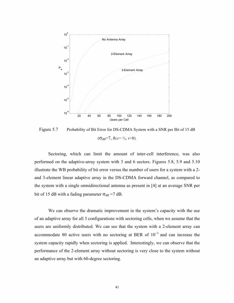
We can see that the system capacity with adaptive arrays can increase the number

of active mobile users for BER of 10−3 or less in a system without an array of 13 to 80

and 125 for a system with 2- and 3-element arrays in Figure 5.7. The capacity gained

from the use of a 2-element adaptive array is an impressive capacity gain of about 600%

over a system without an adaptive array. If a 3-element array is used, the gain in capacity

at the same BER performance is even higher (900%). This demonstrates the strength of

the adaptive-array application in a mobile communication system and its potential for

improving the system’s capacity.

41

20 40 60 80 100 120 140 160 180 20010-6

10-5

10-4

10-3

10-2

10-1

100

Users per Cell

Pe

No Antenna Array

2-Element Array

3-Element Array

Figure 5.7 Probability of Bit Error for DS-CDMA System with a SNR per Bit of 15 dB

(σdB=7, Rcc= ½, v=8).

Sectoring, which can limit the amount of inter-cell interference, was also

performed on the adaptive-array system with 3 and 6 sectors. Figures 5.8, 5.9 and 5.10

illustrate the WB probability of bit error versus the number of users for a system with a 2-

and 3-element linear adaptive array in the DS-CDMA forward channel, as compared to

the system with a single omnidirectional antenna as present in [4] at an average SNR per

bit of 15 dB with a fading parameter σdB =7 dB.

We can observe the dramatic improvement in the system’s capacity with the use

of an adaptive array for all 3 configurations with sectoring cells, when we assume that the

users are uniformly distributed. We can see that the system with a 2-element array can

accommodate 80 active users with no sectoring at BER of 10−3 and can increase the

system capacity rapidly when sectoring is applied. Interestingly, we can observe that the

performance of the 2-element array without sectoring is very close to the system without

an adaptive array but with 60-degree sectoring.

42

20 40 60 80 100 120 140 160 180 20010-8

10-7

10-6

10-5

10-4

10-3

10-2

10-1

100

Users per Cell

Pe

No Sectoring 120-degree Sectoring

60-degree Sectoring

No Sectoring with Array

120-degree Sectoring with Array

60-degree Sectoring with Array

Figure 5.8 Probability of Bit Error for a 2-Element Linear Adaptive Array DS-CDMA

System Using Sectoring with a SNR per Bit of 15 dB (σdB=7, Rcc= ½, v=8).

20 40 60 80 100 120 140 160 180 20010-8

10-7

10-6

10-5

10-4

10-3

10-2

10-1

100

Users per Cell

Pe

No Sectoring 120-degree Sectoring

60-degree Sectoring

No Sectoring with Array

120-degree Sectoring with Array

60-degree Sectoring with Array

Figure 5.9 Probability of Bit Error for a 3-Element Linear Adaptive Array DS-CDMA

System Using Sectoring with a SNR per Bit of 15 dB (σdB=7, Rcc= ½, v=8).

43

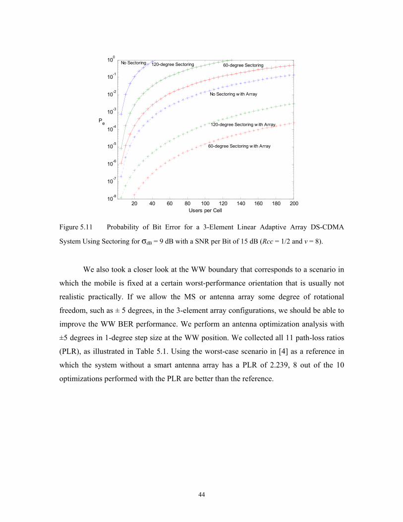
When the adaptive array is applied, the DS-CDMA system can provide good

performance because of interference suppression, which allows it to tolerate other

constraining factors, such as fade depth. If the shadowing parameter σdB is increased to 9

dB, which corresponds to an environment with a deeper fading variation, we can see that

the 2-element array system’s capacity without sectoring will reduce from 80 (σdB = 7) to

30 active users at BER of 10−3 (see Figure 5.10). This is close to a system without an

adaptive array, but with 120-degree sectoring at σdB = 7 dB. For the case of a 3-element

array system, when the shadowing parameter σdB is increased from 7 dB to 9 dB, the

maximum number of active users for the system at BER of 10−3 dropped from 120 to 48,

as in Figure 5.11.

20 40 60 80 100 120 140 160 180 20010-8

10-7

10-6

10-5

10-4

10-3

10-2

10-1

100

Users per Cell

Pe

No Sectoring 120-degree Sectoring 60-degree Sectoring

No Sectoring w ith Array

120-degree Sectoring w ith Array

60-degree Sectoring w ith Array

Figure 5.10 Probability of Bit Error for a 2-Element Linear Adaptive Array DS-CDMA

System Using Sectoring for σdB = 9 dB with a SNR per Bit of 15 dB (Rcc = 1/2 and v = 8).

44

20 40 60 80 100 120 140 160 180 20010-8

10-7

10-6

10-5

10-4

10-3

10-2

10-1

100

Users per Cell

Pe

No Sectoring 120-degree Sectoring 60-degree Sectoring

No Sectoring w ith Array

120-degree Sectoring w ith Array

60-degree Sectoring w ith Array

Figure 5.11 Probability of Bit Error for a 3-Element Linear Adaptive Array DS-CDMA

System Using Sectoring for σdB = 9 dB with a SNR per Bit of 15 dB (Rcc = 1/2 and v = 8).

We also took a closer look at the WW boundary that corresponds to a scenario in

which the mobile is fixed at a certain worst-performance orientation that is usually not

realistic practically. If we allow the MS or antenna array some degree of rotational

freedom, such as ± 5 degrees, in the 3-element array configurations, we should be able to

improve the WW BER performance. We perform an antenna optimization analysis with

±5 degrees in 1-degree step size at the WW position. We collected all 11 path-loss ratios

(PLR), as illustrated in Table 5.1. Using the worst-case scenario in [4] as a reference in

which the system without a smart antenna array has a PLR of 2.239, 8 out of the 10

optimizations performed with the PLR are better than the reference.

45

Table 5.1 3-Element Array Path-Loss Ratio Values for Different Orientation Offset

in the WW Case

0.5

1

1.5

30

210

60

240

90

270

120

300

150

330

180 0

SBS

IBS 1

IBS 6

Orientation Offset Path Loss Ratio

+5 1.3518

+4 1.3588

+3 1.4300

+2 9.2091

+1 10.6014

WW case 19.8476

−1 1.0877

−2 1.1107

−3 1.3611

−4 1.3560

−5 1.3532

46

Figure 5.12 Antenna Factor of the WW Case for a 3-Element Array Antenna with a

Path-Loss Ratio of 19.8476

0.5

1

1.5

2

30

210

60

240

90

270

120

300

150

330

180 0

SBS

IBS 6

IBS 1

Figure 5.13 Antenna Factor of the WW Case for a 4-Element Array Antenna at −1

Degree Offset with a Path-Loss Ratio of 1.0877

Figure 5.12 shows the antenna factor for the WW location (R =0.866, A=90

degree) at array orientation of 2 degrees for a 3-element linear array. Figure 5.13 shows

the antenna factor when the array is rotated for −1 degree. We can observe that the array

factor patterns are significantly different with just 1-degree difference in orientation. We

repeat the analysis process at the WW case position for the 2-element and 3-element

array. We observed similar characteristics where the WW-case Path-Loss Ratio is

reduced significantly within a small ±5 degree orientation offset, which is reasonable in a

practical implementation. Hence the Worst-Worst case BER performance can be

improved significantly with such a practical allowance. Table 5.2 shows that we can

obtain many path-loss ratios that are less than the worst-case situation for a DS-CDMA

system without a linear array of 2.239. Hence with the ± 5 degrees of orientation offset,

we can observe that the worst performance of a system with the linear array in practice

will always be better than a system without the smart antenna.

47

Table 5.2 Path-Loss Ratio Values of a 2-, 3- and 4-Element Array with a Different

Orientation Offset at the WW Case

In Figures 5.14 to Figure 5.16, we observe similar characteristics for a 4-element

array system with a few degrees of orientation offset in the WW case position. We can

see drastic changes in antenna factor patterns that allow the system to reduce the PLR

significantly from 185.6 when the array is rotated by +1 or –2 degrees to 0.795 and

0.6293 respectively.

Orientation Offset Path-Loss Ratio

2-Element Array 3-Element Array 4-Element Array

+5º 0.6147 1.3518 1.8762

+4º 0.5983 1.3588 2.0265

+3º 0.5826 1.4300 6.1393

+2º 0.8634 9.2091 7.8293

+1º 0.8634 10.6014 0.7950

WW case 661.2276 19.8476 185.6

−1º 6.3172 1.0877 12.8122

−2º 3.1465 1.1107 0.6293

−3º 2.0834 1.3611 5.4201

−4º 1.5512 1.3560 3.9677

−5º 1.2318 1.3532 3.0803

48

Figure 5.14 Antenna Factor of the WW Case for a 4-Element Array Antenna with a

Path-Loss Ratio of 185.6

Figure 5.15 Antenna Factor of the WW Case for a 4-Element Array Antenna at +1

Degree Offset with a Path-Loss Ratio of 0.7950

49

Figure 5.16 Antenna Factor of the WW Case for a 4-Element Array Antenna at

−2 Degree Offset with a Path-Loss Ratio of 0.6293

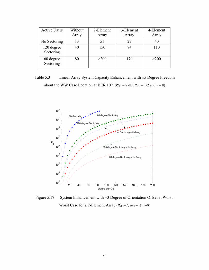
In Figures 5.17 to 5.19, the DS-CDMA system’s BER performance with a

different number of elements array within ±5 degrees of the WW case orientation is

illustrated. This is used to compare the worst-case performance of a system without an

array as in [4]. The comparisons demonstrate the strength of the optimization algorithm,

which allows the system to escape the WW case with good system performance with a

small change in the orientation angle. We can see that the practical worst case of a 4-

element array system without any sectoring has the same capacity as a system without an

array but with 120-degree sectoring. However when 120-degree sectoring is used in the

4-element array system, the system capacity of 110 active users exceeds the maximum

capacity of 80 active users of the system without an array but with 60-degree sectoring.

Table 5.3 summarized the simulation results.

50

Table 5.3 Linear Array System Capacity Enhancement with ±5 Degree Freedom

about the WW Case Location at BER 10−3 (σdB = 7 dB, Rcc = 1/2 and v = 8)

20 40 60 80 100 120 140 160 180 20010-8

10-7

10-6

10-5

10-4

10-3

10-2

10-1

100

Users per Cell

Pe

No Sectoring 60 degree Sectoring

120 degree Sectoring

No Sectoring w ithArray

120 degree Sectoring w ith Array

60 degree Sectoring w ith Array

Figure 5.17 System Enhancement with +3 Degree of Orientation Offset at Worst-

Worst Case for a 2-Element Array (σdB=7, Rcc= ½, v=8)

Active Users Without Array

2-Element Array

3-Element Array

4-Element Array

No Sectoring 13 51 27 40 120 degree Sectoring

40 150 84 110

60 degree Sectoring

80 >200 170 >200

51

20 40 60 80 100 120 140 160 180 20010-8

10-7

10-6

10-5

10-4

10-3

10-2

10-1

100

Users per cell

Pe

No Sectoring

120-degree Sectoring

60-degree Sectoring

No sectoring w ith Array

120-degree Sectoring w ith Array

60-degree Sectoring w ith Array

Users per Cell

Figure 5.18 System Enhancement with −1 Degree of Orientation Offset in the Worst-

Worst Case for a 3-Element Array (σdB=7, Rcc= ½, v=8)

20 40 60 80 100 120 140 160 180 20010-8

10-7

10-6

10-5

10-4

10-3

10-2

10-1

100

Users per Cell

Pe

No Sectoring 120-degree Sectoring

No Sectoring w ith Array

60-degree Sectoring

120-degree Sectoring w ith Array

60-degree Sectoring w ith Array

Figure 5.19 System Enhancement with +1 Degree of Orientation Offset in the Worst-

Worst Case for a 4-Element Array (σdB=7, Rcc= ½, v=8)

52

We have demonstrated that with 2- and 3-element linear arrays, we can improve the

maximum number of active users per cell at SNR per bit of 15 dB with a shadowing of

σdB =7 dB to 600% and 900% respectively, higher than a system without the linear array.

Different sectorings were also performed on the system, which can dramatically improve

the system’s capacity. Our analyses in this chapter assumed that the antenna perform

identically at all frequencies. This may be true for narrow–band channel. For a wide-band

channel, we would need the application of tapped-delay line (transversal filter) be

employed to equalize the frequency varying effect. Chapter VI presents the application

and performance analysis of the tapped-delay line in our DS-CDMA mobile

communication system.

53

VI PERFORMANCE ANALYSIS OF WIDEBAND ADAPTIVE ANTENNA

SYSTEM

Earlier we assumed that our DS-CDMA system under analysis is a narrowband

system. The presence of a single complex adaptive weight in each element channel of an

adaptive array is sufficient for processing narrowband signals. However, the processing

of broadband signals, such as the forward channel of a 3G DS-CDMA network, requires

that tapped-delay line (transversal filter) be employed in each element channel. In a

practical implementation, every channel is slightly different electrically, which leads to

channel mismatching. This mismatch could cause significant differences in frequency

response characteristics from channel to channel and may severely degrade the array

performance. Figure 6.1 shows the block diagram of the K-element antenna with L-

tapped-delay line system

1

K

X1(t)

W11*

WK1*

XK(t)

X1(t-(l-1)∆)

(L-1) Tap Point L TapPoint

W1l* W1(L-1)

* W1L*

X1(t-(L-1)∆) X1(t-L∆)

XK(t-(l-1)∆)

(L-1) Tap Point L TapPoint

WKl* WK(L-1)

* WKL*

XK(t-(L-1)∆) XK(t-L∆)

y(t)

Figure 6.1 Wideband K-Element Array with an L-Tapped-Delay Line

54

The output of array, y(t), is defined as:

∑∑L K

* *kl k

l=1 k=1(t)= w x (t -(l -1)∆)=W X(t)y (4.18)

where

.

(1)11 1L

(2)

(1) (L)

(L)K1 KL

W w wW . .

W = . , W = . , .... W = . . . .

w wW

(1)1 1

1(2)

(1) (2) (L)

(L)K K

X (t) x (t) x (t - ∆)x (t - (L - 1)∆)

X (t) . .

X(t)= . , X (t)= . ,X (t)= . , . . . . X (t)= . . .

x (t) x (t - ∆)X (t)

K

. .X (t - (L - 1)∆)

The transfer function H(f) can be defined by taking the Fourier transform of the above y(t).

∑ ∑ kl

L K* i2πf[(k -1)τ+(l-1)∆]

l=1 k=1

(f) = w eX(f)YH(f)= (4.19)

where

δ sin θτ =v

and ∆ is the inter-tap delay spacing (in our analysis using 2- and 3-tapped-delay line,

∆=λo/4), v is the speed of light and δ is the linear antenna array separation, and θ is the

direction of arrival of the signal (desired or interference).

We see that an array system with tapped-delay line may be able to equalize the

broadband signal, but we need a more complex algorithm and more computational power

to determine an optimized set of weights. In the case of a 3-element linear array, we need

55

to obtain 6 weight values whereas a 3-element, 3-tapped delay line system requires 18

weight values. We must note that the amount of time to determine a set of optimized

weights increases significantly with the number of taps, which is critical for

implementation. Hence the number of taps for a tapped-delay line implementation should

be minimized to conserve electrical power and evaluation time.

We now apply tapped-delay line (transversal filter) processing to each antenna

element channel to allow frequency-dependent amplitude and phase adjustments for the

broadband signals. The use of a tapped-delay line thereby provides the capability of

equalizing the frequency varying effect on the antenna array when the latter is receiving a

broadband signal. The performance of a DS-CDMA cellular system with a mobile-

terminal equipped with a linear array tapped-delay line was analyzed and performed.

We perform optimization by minimizing the ISR at the center nominal frequency

of the signals. The angle of arrival for the desired (SBS) signal and interference were

assumed to be known and is used to determine the optimized complex weight values for

the tapped-delay line. Figure 6.2 and Figure 6.3 show the optimized transfer functions

H(f) in (4.19) of a 2-element linear array with a 2- and 3-tapped delay line at 4%

bandwidth of the nominal center frequency. We can see that the optimized desired signal

base-station (SBS) remains flat over the 4% bandwidth width while the transfer functions

of the interference base-station (IBS) may fluctuate significantly over the same

bandwidth. Although at the nominal center frequency, we may achieve excellent ISR

suppression greater than –70 dB (3-tap case with IBS1 as the main suppressed interferer),

at the lower 4% band-edge we can only achieve about −16 dB of ISR.

56

1.96 1.97 1.98 1.99 2 2.01 2.02 2.03 2.04-30

-25

-20

-15

-10

-5

0

5

10

Frequency [GHz]

H(f) [dB]

SBS (Desired Signal)

IBS 3 IBS 4 IBS 5

IBS 6 IBS 1

IBS 2

Figure 6.2 Desired Signal (SBS) and Interference Signal (IBS) Transfer Functions of

a 2-Element Array with a 2-Tapped-Delay Line System and 4% Bandwidth

1.96 1.97 1.98 1.99 2 2.01 2.02 2.03 2.04-60

-50

-40

-30

-20

-10

0

10

Frequency [GHz]

H(f) [dB]

IBS 2..5

SBS

IBS 6

IBS 1

Figure 6.3 Desired Signal (SBS) and Interference Signal (IBS) Transfer Functions of

a 2-Element Array with a 3-Tapped-Delay Line System and 4% Bandwidth

57

20 40 60 80 100 120 140 160 180 20010-8

10-7

10-6

10-5

10-4

10-3

10-2

10-1

100

Users per Cell

Pe

Without Array

2-element Array (Narrow Band)

2-element Array with 2-Tap

2-element Array with 3-Tap

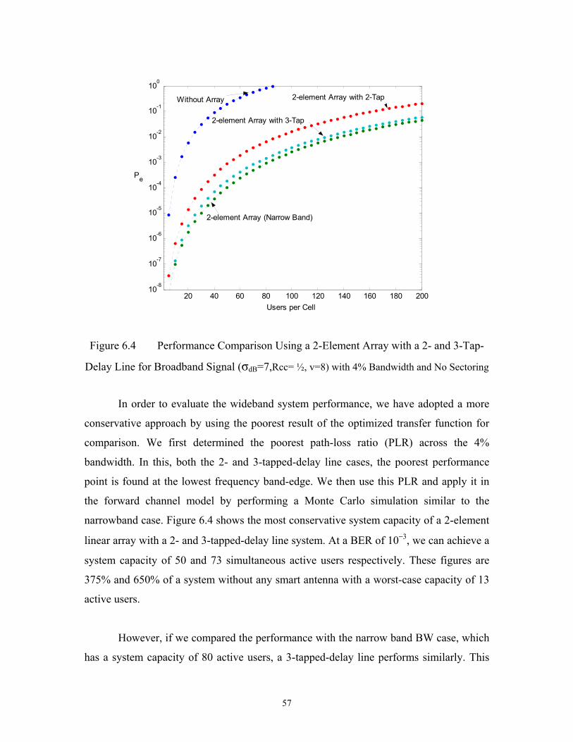
Figure 6.4 Performance Comparison Using a 2-Element Array with a 2- and 3-Tap-

Delay Line for Broadband Signal (σdB=7,Rcc= ½, v=8) with 4% Bandwidth and No Sectoring

In order to evaluate the wideband system performance, we have adopted a more

conservative approach by using the poorest result of the optimized transfer function for

comparison. We first determined the poorest path-loss ratio (PLR) across the 4%

bandwidth. In this, both the 2- and 3-tapped-delay line cases, the poorest performance

point is found at the lowest frequency band-edge. We then use this PLR and apply it in

the forward channel model by performing a Monte Carlo simulation similar to the

narrowband case. Figure 6.4 shows the most conservative system capacity of a 2-element

linear array with a 2- and 3-tapped-delay line system. At a BER of 10−3, we can achieve a

system capacity of 50 and 73 simultaneous active users respectively. These figures are

375% and 650% of a system without any smart antenna with a worst-case capacity of 13

active users.

However, if we compared the performance with the narrow band BW case, which

has a system capacity of 80 active users, a 3-tapped-delay line performs similarly. This

58

demonstrates that if we could obtain a set of optimized weights for the tapped-delay line

to equalize the broadband signal effectively, we could achieve a similar performance

level as those in the narrow-band adaptive antenna system. As the complexity to

determine the optimized weights of the adaptive tapped-delay line system increases

exponentially with the number of taps used, in the case of the 2-element array, a 3-

tapped-delay line may be sufficient to equalize the broadband signal while effectively

suppressing the interference.

We repeat the process to obtain the optimum transfer functions for the 3-element

array system with 2- and 3-tapped-delay line, as in Figures 6.5 and 6.6. In this 3-element

array system, we determine the most conservative PLR is at the lowest frequency band-

edge for a 2-tap case and at the highest frequency band-edge for a 3-tap case. Both PLR

computed in this case are fairly close to each other. Figure 6.7 illustrates the system

performance. We see that both 2- and 3-tap systems have similar performance, as their

optimized path-loss ratios are only slightly different in magnitude. We can also see that

both broadband cases outperform the narrowband case significantly (>200 active users).

In the broadband 3-element antenna case, a 2-tapped-delay line should suffice to equalize

the signal while providing superior system performance over the narrowband system. In this chapter, we have evaluated the performance of a tapped-delay line

application in a DS-CDMA mobile communication system. We are able to equalize the

frequency varying effect of the broadband signal using tapped-delay-line. In a 2-element

linear-array system, 3 taps would be sufficient to equalize the broadband signal while

providing a similar performance level of a narrowband adaptive-array system. In the case

of a 3-element linear-array system, 2 taps would suffice.

59

1.96 1.97 1.98 1.99 2 2.01 2.02 2.03 2.04-140

-120

-100

-80

-60

-40

-20

0

20

Frequency [GHz]

H(f) [dB]

SBS (Desired Signal)

IBS 3

IBS 1,IBS 2 IBS 4, IBS5, IBS 6

Figure 6.5 Desired Signal (SBS) and Interference Signal (IBS) Transfer Functions of

a 3-Element Array with a 2-Tapped-Delay Line System and 4% Bandwidth

1.96 1.97 1.98 1.99 2 2.01 2.02 2.03 2.04-140

-120

-100

-80

-60

-40

-20

0

20

Frequency [GHz]

H(f) [dB]

SBS (Desired Signal)

IBS 2 IBS 4

IBS 5 IBS 3

IBS 6 IBS 1

Figure 6.6 Desired Signal (SBS) and Interference Signal (IBS) Transfer Functions of

a 3-Element Array with a 3-Tapped-Delay Line System and 4% Bandwidth

60

20 40 60 80 100 120 140 160 180 20010-8

10-7

10-6

10-5

10-4

10-3

10-2

10-1

100

Users per Cell

Pe

Without Array

2-element Array (Narrow Band)

2-Element Array with 2-Taps

2-element Array with 3-Taps

Figure 6.7 Performance Comparison Using a 3-Element Array with a 2- and 3-

Tapped-Delay Line for Broadband Signal (σdB=7, Rcc= ½, v=8) with 4% Bandwidth and No

Sectoring

61

VII CONCLUSIONS AND FUTURE WORK

A. CONCLUSIONS

In this thesis, we have applied an adaptive linear array at the mobile user terminal

for a wideband DS-CDMA mobile communication system. A performance analysis was

performed with a focus on the forward channel of the DS-CDMA system in a log-normal

shadowing and Rayleigh slow flat-fading environment. The application of the adaptive

linear antenna array compounded the problem of obtaining a representative system

performance boundary because the mobile terminal can be randomly located anywhere in

the cell and the antenna array is orientation limited. Further, the performance of the array

may also vary significantly with a small change in orientation.

We used 2-, 3-, and 4-element linear arrays to evaluate the overall system’s

performance. Four performance boundaries (BB, WB, WW, BW) were established for

each number of the linear arrays to compare and to evaluate the system’s performance.

These boundaries were reviewed and we determined that for a worst-case performance

comparison, the WB case would be the tightest performance boundary for an array that

can be orientated 360 degrees. In the case of a 2- or 3-element array system, the number

of active users per cell that can be supported at SNR per bit of 15 dB with a shadowing of

σdB =7 dB is 600% and 900%, respectively, higher than a system without the linear array.

Different sectorings were also performed on the system, which can dramatically improve

the system’s capacity.

The application of the adaptive array has allowed the DS-CDMA system to

perform better because of its superior interference suppression and this allows it to

tolerate other constraining factors, such as higher fade depth.

To illustrate a practical implementation with ±5 degree freedom, when the array

cannot orientate 360 degrees freely, all 3 different element array systems can still assure a

system capacity enhancement of between 200% to 400% over the worst-case system

62

capacity for one that does not use any array. The adaptive array system has also

demonstrated its versatility in providing a dramatic array performance enhancement with

a small change of array orientation.

The performance of the adaptive-array system for a broadband signal is also

evaluated with the use of a tapped-delay line. It has been demonstrated that the

optimization process has been extremely computationally expensive and hence minimum

taps should be used for practical consideration. The result obtained also illustrated that,

in general, for a 2-element linear-array system, 3 taps would be sufficient to equalize the

broadband signal while providing a similar performance level of a narrowband adaptive-

array system. In the case of a 3-element linear-array system, 2 taps would suffice.

B. FUTURE WORK

As a future research subject, the DS-CDMA system performance analysis with an

adaptive array in a Rayleigh fading and log-normal slow fading environment can be

extended to a system with a circular array antenna. two-dimensional or even three-

dimensional time and an angle-of-arrival geometric model can also be incorporated into

the system’s performance analysis.

63

LIST OF REFERENCES

[1] Y. Okumura, "Field Strength and Its Variability in VHF and UHF Land Mobile Radio

Service,” Reviews of the Electrical Communications Laboratory (Japan), vol. 16, no. 9-

10. pp. 825-873, September-October 1968.

[2] COST 231,”Urban Transmission Loss Models for Mobile Radio in the 900 and 1800

MHz bands(Rev. 2),” COST 231 TD(90) 119 Rev. 2, The Hague, September 1991.

[3] John G. Proakis, Digital Communications, 4th Edition, McGraw Hill, 2001.

[4] J.E Tighe, “Modeling and Analysis of Cellular CDMA Forward Channel,” PhD

Dissertation, Naval Postgraduate School, Monterey, CA, March 2001.

[5] Ramakrishna Janaswamy, Radiowave Propagation and Smart Antennas for Wireless

Communications, Kluwer Academic 2001.

[6 ] Ayman F. Naguib “Adaptive Antennas for CDMA Wireless Networks,” PhD

Dissertation, Stanford University, CA, August 1996.

[7] Theodore S. Rappaport, Wireless Communications Principle and Practice, 2nd

Edition, Prentice Hall, 2002.

[8] Robert A. Monzingo and Thomas W. Miller, Introduction to Adaptive Arrays, New

York:Wiley, 1980.

[9] Kaiser Tan B.K., “Performance Analysis of Adaptive Antenna with Coding and

RAKE Receiver,” MSc Dissertation, Naval Postgraduate School, Monterey, CA, March

2002.

64

THIS PAGE INTENTIONALLY LEFT BLANK

65

INITIAL DISTRIBUTION LIST

1. Defense Technical Information Center

Ft. Belvoir, VA

2. Dudley Knox Library

Naval Postgraduate School

Monterey, CA

3. Chairman

Department of Electrical and Computing Engineering

Naval Postgraduate School

Monterey, CA

3. Professor Tri T. Ha

Department of Electrical and Computing Engineering

Naval Postgraduate School

Monterey, CA

4. Professor Jovan Lebaric

Department of Electrical and Computing Engineering

Naval Postgraduate School

Monterey, CA

5. Kok Keng Ng

Blk 285A Toh Guan Road, #15-56, #15-56. Singapore 601285