SMART CONTROL OF CANTILEVER STRUCTURES …ijssst.info/Vol-07/No-4-5/Paper7.pdf · as they may...

T.C. MANJUNATH and B. BANDYOPADHYAY : SMART CONTROL OF CANTILEVER STRUCTURES

I.J. of SIMULATION Vol. 7 No 4-5 51 ISSN 1473-804x online, 1473-8031 print

SMART CONTROL OF CANTILEVER STRUCTURES USING OUTPUT FEEDBACK

T.C. MANJUNATH, B. BANDYOPADHYAY

Interdisciplinary Programme in Systems & Control Engineering,

101 B, ACRE Building, Indian Institute of Technlogy Bombay, Powai, Mumbai - 400076, Maharashtra, India.

Email : [email protected] ; [email protected] URL : http://www.sc.iitb.ac.in/~tcmanju ; http://www.sc.iitb.ac.in/~bijnan

Phone : +91 22 25767884 ; +91 22 25767889 ; Fax : +91 22 25720057

Abstract : This paper features the modelling and design of a type of multirate output feedback based controller (Fast Output Sampling Feedback - FOS) to control the flexural vibrations of a smart flexible Timoshenko cantilever beam for a Single Input Single Output (SISO) case by retaining the first 2 dominant vibratory modes. Piezoelectric patches are bonded as sensor / actuator to the master structure at different finite element locations along the length of the beam. The beam structure is modelled in state space form using the concept of piezoelectric theory, the Timoshenko beam theory and the Finite Element Method (FEM) technique and by dividing the beam into 4 finite elements and placing the piezoelectric sensor / actuator at one discrete location as a collocated pair at a time, i.e., as surface mounted sensor / actuator, say, at FE position 1 or 2 or 3 or 4, thus giving rise to 4 SISO models of the same plant. FOS feedback controllers are designed for the above 4 models of the same plant. The piezo sensor / actuator pair is moved from the free end to the fixed end of the beam. The effect of placing the collocated sensor / actuator pair at various finite element locations along the length of the beam is observed and the conclusions are drawn for the best performance and for the smallest magnitude of the control input required to control the vibrations of the flexible beam. Keywords : Smart structure, Timoshenko, FOS, FEM, State space model, Vibration control, LMI. 1. INTRODUCTION Active vibration control is an important problem in structures. One of the ways to tackle this problem is to make the structure smart, intelligent, adaptive and self-controlling. The main objective of Active Vibration Control (AVC) is to reduce the vibration of a system by automatic modification of the system’s structural response. In many situations, it is important to minimize these structural vibrations, as they may affect the stability and performance of the structures. This obviates the need to strengthen the structure from dynamic forces and disturbances in order to minimize the effects of vibrations and enables the development of lighter, often-cheaper structures exhibiting superior performance. Thus, the vibration control of any system is always a formidable challenge for any system designer. Any AVC system consists of a plant, actuator, sensor and a controller. Sensors and actuators together integrated into the structure is what is called as a “Smart Structure”. The need for such intelligent structures called as smart structures [Culshaw, 1992] arises because of their high performances in numerous structural applications. Such intelligent structures incorporate smart materials called as actuators and sensors (based on Piezoelectrics, Magneto-Rheological

Fluids, Piezoceramics, Electro-Rheological Fluids, Shape Memory Alloys, PVDF, Optical fibers, etc.) that are highly integrated into the structure and have structural functionality, as well as highly integrated control logic, signal conditioning and power amplification electronics. These materials can be used to generate a secondary vibrational response in a mechanical system which has the potential to reduce the overall response of the system plant by the destructive interference with the original response of the system, caused by the primary source of vibration. Active control of vibrations in flexible structures through the smart structure concept is a developing area of research and has numerous applications, especially in the vibration control of structures (such as beams, plates, shells), in aerospace engineering, flexible robot manipulators, antennas, active noise control, shape control and in earthquakes. Research on smart structures is interdisciplinary because it involves materials, structural mechanics, electronics, signal processing, communication, mathematics and control. The goal of this multi-disciplinary research is to develop techniques to design, control, analyze, and visualize optimal or near optimal smart and adaptive structures using smart materials. A specific area discussed in this paper is particularly pertinent to the recent new research developments carried out

T. C. MANJUNATH and B. BANDYOPADHYAY : SMART CONTROL OF CANTILEVER STRUCTURES


by the authors in the field of modelling and control of smart structures (flexible Timoshenko cantilever beams with integrated surface mounted collocated sensors and actuators) in the institute. Considerable interest is focused on the modelling, control and implementation of smart structures using Euler-Bernoulli beam theory and Timoshenko Beam theory with integrated piezoelectric layers in the recent past. In Euler Bernoulli beam theory (classical beam model), the assumption made is, before and after bending, the plane cross section of the beam remains plane and normal to the neutral axis. Since the shear forces, axial displacement are neglected in Euler-Bernoulli theory, slightly inaccurate results may be obtained. Timoshenko Beam Theory is used to overcome the drawbacks of the Euler-Bernoulli beam theory by considering the effect of shear and axial displacements. In the Timoshenko beam theory, cross sections remains plane and rotate about the same neutral axis as the Euler-Bernoulli model, but do not remain normal to the deformed longitudinal axis. The deviation from normality is produced by a transverse shear that is assumed to be constant over the cross section. The total slope of the beam in this model consists of two parts, one due to bending θ, and the other due to shear β. Thus, the Timoshenko Beam model is superior to Euler-Bernoulli model in precisely predicting the beam response. Thus, this model corrects the classical beam model with first-order shear deformation effects. The following few paragraphs gives a deep insight into the research work done on the intelligent structures using the 2 types of theories so far. Culshaw [1992] discussed the concept of smart structure, its benefits and applications. Rao and Sunar [1994] explained the use of piezo materials as sensors and actuators in sensing vibrations in a survey paper. Baily and Hubbard [1985] have studied the application of piezoelectric materials as sensor / actuator for flexible structures. Hanagud et.al. [1992] developed a Finite Element Model (FEM) for a beam with many distributed piezoceramic sensors / actuators. Fanson et.al. [1990] performed some experiments on a beam with piezoelectrics using positive position feedback. Balas [1978] did extensive work on the feedback control of flexible structures. Experimental evaluation of piezoelectric actuation for the control of vibrations in a cantilever beam was presented by Burdess et.al. [1992]. Brenan et.al. [1999] performed some experiments on the beam for different actuator technologies. Yang and Lee [1993] studied the optimization of feedback gain in control system design for structures. Crawley and Luis [1987] presented the development of

piezoelectric sensor / actuator as elements of intelligent structures.

Hwang and Park [1993] presented a new finite element (FE) modelling technique for flexible beams. Continuous time and discrete time algorithms were proposed to control a thin piezoelectric structure by Bona, et.al. [1997]. Schiehlen and Schonerstedt [1998] reported the optimal control designs for the first few vibration modes of a cantilever beam using piezoelectric sensors / actuators. S. B. Choi et.al. [1995] have shown a design of position tracking sliding mode control for a smart structure. Distributed controllers for flexible structures can be seen in Forouza Pourki [1993]. Shiang Lee [1996] devised a new form of control strategy for vibration control of smart structures using neural networks. A passivity-based control for smart structures was designed by Gosavi and Kelkar [2004]. A self tuning active vibration control scheme in flexible beam structures was carried out by Tokhi [1994]. Active control of adaptive laminated structures with bonded piezoelectric sensors and actuators was investigated by Moita et.al. [2004]. Ulrich et. al. [2002] devised a optimal LQG control scheme to suppress the vibrations of a cantilever beam. Finite element simulation of smart structures using an optimal output feedback controller for vibration and noise control was performed by Young et.al. [1999]. Work on vibration suppression of flexible beams with bonded piezo-transducers using wave-absorbing controllers was done by Vukowich and Koma [2000]. Aldraihem et. al. [1997] have developed a laminated beam model using two theories; namely, Euler-Bernoulli beam theory and Timoshenko Beam theory. Abramovich [1998] has presented analytical formulation and closed form solutions of composite beams with piezoelectric actuators, which was based on Timoshenko beam theory. He also studied the effects of actuator location and number of patches on the actuator’s performance for various configurations of the piezo patches and boundary conditions under mechanical and / or electric loads. Using a higher-order shear deformation theory, Chandrashekhara and Varadarajan [1997] presented a finite element model of a composite beam to produce a desired deflection in beams with clamped-free, clamped-clamped and simply supported ends. Sun and Zhang [1995] suggested the idea of exploiting the shear mode to create transverse deflection in sandwich structures. Here, he proved that embedded shear actuators offer many advantages over surface mounted extension actuators. Aldraihem and Khdeir [2000] proposed analytical models and exact solutions for beams with shear and extension piezoelectric actuators and the



models were based on Timoshenko beam theory and higher-order beam theory. Exact solutions were obtained by using the state-space approach. Doschner and Enzmann [1998] designed a model-based controller for smart structures. Robust multivariable control of a double beam cantilever smart structure was implemented by Robin Scott et. al. [2003]. In a more recent work, Zhang and Sun [1996] formulated an analytical model of a sandwich beam with shear piezoelectric actuator that occupies the entire core. The model derivation was simplified by assuming that the face layers follow Euler-Bernoulli beam theory, whereas the core layer obeys Timoshenko beam theory. Furthermore, a closed form solution of the static deflection was presented for a cantilever beam. A new method of modeling and shape control of composite beams with embedded piezoelectric actuators was proposed by Donthireddy and Chandrashekhara [1996]. A model reference method of controlling the vibrations in flexible smart structures was shown by Murali et.al. [1995]. Thomas and Abbas [1975] explained some techniques of performing finite element methods for dynamic analysis of Timoshenko beams. A FEM approach was used by Benjeddou et al. [1999] to model a sandwich beam with shear and extension piezoelectric elements. The finite element model employed the displacement field of Zhang and Sun [1996]. It was shown that the finite element results agree quite well with the analytical results. Deflection analysis of beams with extension and shear PZT patches using discontinuity functions was proposed by Ahmed and Osama in [2001]. Raja et. al. [2002] extended the finite element model of Benjeddou’s research team to include a vibration control scheme. Azulay and Abramovich [2004] have presented analytical formulation and closed form solutions of composite beams with piezoelectric actuators. Abramovich and Lishvits [1994] did extensive work on cross-ply beams to control the free vibrations. An improved 2-node Timoshenko beam model incorporating the axial displacement and shear was presented by Kosmataka and Friedman [1993] which is used in our work for the controller design. The outline of the paper is as follows. A brief review of related literature about the types of beam models was given in the introductory section. Section 2 gives a overview into the modelling technique (sensor / actuator model, finite element model, state space model) of the smart cantilever beam modelled using Timoshenko beam theory. A brief review of the controlling technique, viz., the fast output sampling feedback control technique is presented in

section 3, followed by the design of controller for the first two vibratory modes for the 4 types of SISO models. The simulation results are presented in Section 5. Conclusions are drawn in Section 6 followed by the references.

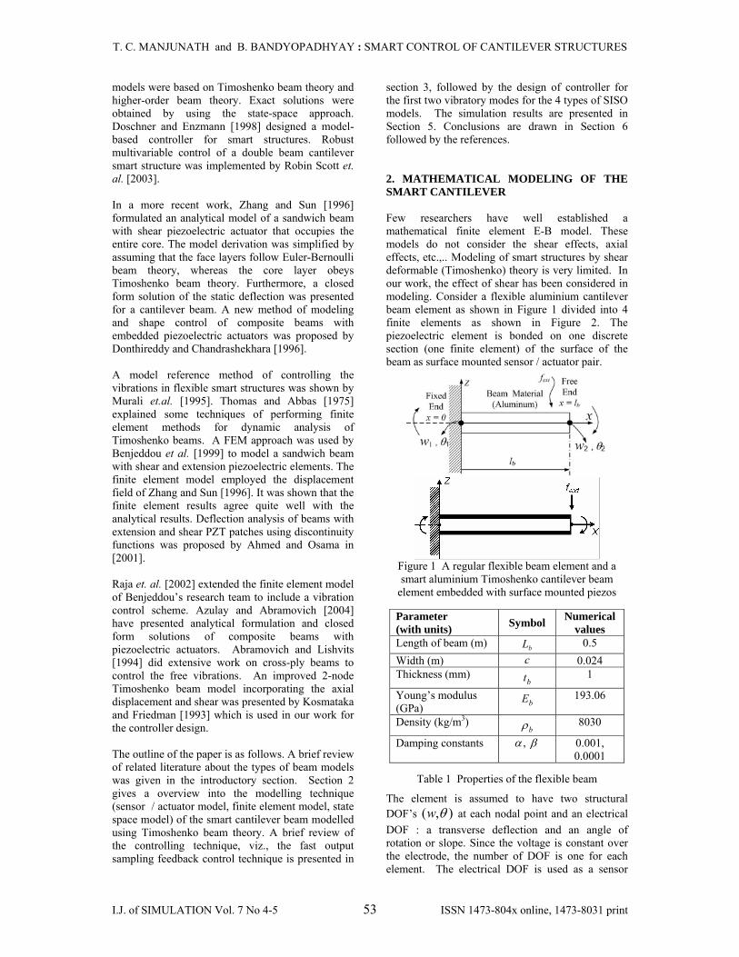
2. MATHEMATICAL MODELING OF THE SMART CANTILEVER Few researchers have well established a mathematical finite element E-B model. These models do not consider the shear effects, axial effects, etc.,.. Modeling of smart structures by shear deformable (Timoshenko) theory is very limited. In our work, the effect of shear has been considered in modeling. Consider a flexible aluminium cantilever beam element as shown in Figure 1 divided into 4 finite elements as shown in Figure 2. The piezoelectric element is bonded on one discrete section (one finite element) of the surface of the beam as surface mounted sensor / actuator pair.

Figure 1 A regular flexible beam element and a smart aluminium Timoshenko cantilever beam

element embedded with surface mounted piezos

Parameter (with units) Symbol Numerical

values Length of beam (m) bL 0.5 Width (m) c 0.024

Thickness (mm) bt 1

Young’s modulus (GPa) bE 193.06

Density (kg/m3) bρ 8030

Damping constants βα , 0.001, 0.0001

Table 1 Properties of the flexible beam

The element is assumed to have two structural DOF’s ),( θw at each nodal point and an electrical DOF : a transverse deflection and an angle of rotation or slope. Since the voltage is constant over the electrode, the number of DOF is one for each element. The electrical DOF is used as a sensor



voltage or actuator voltage. Corresponding to the two DOF’s, a bending moment acts at each nodal point, i.e., counteracting moments are induced by the piezoelectric patches. The bending moment resulting from the voltage applied to the actuator adds a positive finite element bending moment, which is the moment at node 1, while subtracting it at node 2.

Parameter (with units) Symbol Numerical

values Length (m)

pl 0.125

Width (m) b 0.024

Thickness (mm) sa tt , 0.5

Young’s modulus (GPa) pE 68

Density (kg/m3) pρ 7700

Piezo strain constant (m /V) 31d 1210125 −×

Table 2 Properties of the piezoelectric element

In modelling of the smart beam, the following assumptions are made. The mass and stiffness of the adhesive used to bond the sensor / actuator pair to the master structure is being neglected. The smart cantilever beam model is developed using 1 piezoelectric beam element, which includes sensor and actuator dynamics and remaining beam elements as regular beam elements based on Timoshenko beam theory assumptions. The cable capacitance between the piezo patches and the signal-conditioning device is considered negligible and the temperature effects are neglected. The signal conditioning device gain is assumed as 100. An external force input extf (impulse) is applied at the free end of the smart beam. The beam is subjected to vibrations and takes a lot of time for the vibrations to dampen out. These vibrations are suppressed quickly in no time by the closed loop action of the controller, sensor and actuator. Thus, there are two inputs to the plant. One is the external force input extf (impulse disturbance), which is taken as a load matrix of 1 unit in the simulation and the other input is the control input u to the actuator from the FOS controller. The dimensions and properties of the aluminium cantilever beam and piezoelectric sensor / actuator used are given in Tables 1 and 2 respectively. 2.1 Finite Element Modelling of The Regular Beam Element A regular beam element is shown in Figure 1. The longitudinal axis of the regular beam element lies along the X-axis. The beam element has constant moment of inertia, modulus of elasticity, mass

density and length. The displacement relations in the zyx and, directions of the beam can be written as [Friedman and Kosmataka, 1993], [Manjunath and Bandyopadhyay, 2005]

,)(),(),,,( ⎟⎠⎞

⎜⎝⎛ −∂∂

== xxwztxztzyxu βθ (1)

,0),,,( =tzyxv (2) ),,(),,,( txwtzyxw = (3)

Figure 2(a) Model 1 ( PZT placed at FE 1, root)

Figure 2(b) Model 2 ( PZT placed at FE 2)

Figure 2(c) Model 3 ( PZT placed at FE 3, free end)

Figure 2(d) Model 2 ( PZT placed at FE 4)

Figure 2 A SISO smart Timoshenko beam divided into 4 finite elements and the sensor / actuator pair

moved from fixed end to free end where w is the time dependent transverse displacement of the centroidal axis (along z -axis),θ is the time dependent rotation of the beam cross-section about y -axis, u is the axial displacement along the x -axis, v is the lateral displacement along the y -axis which is equal to zero. The total slope of the beam consists of two



parts, one due to bending, which is )(xθ and the other due to shear, which is )(xβ . The axial displacement of a point at a distance z from the centre line is only due to the bending slope and the shear slope has no contribution to this. The strain components of the beam are given as

,εx

zx

uxu

xx ∂∂

=∂∂

∂∂

=∂∂

=θθ

θ (4)

,ε 0=∂∂

=yv

yy (5)

,ε 0=∂∂

=zw

zz (6)

where , ,xx yy zzε ε ε are the longitudinal strains or the tensile strains in the 3 directions, i.e., in the

, ,x y z directions. The shear strains γ induced in the beam along the 3 directions (viz., along

, ,x y z directions) are given by

,21

21

⎥⎦⎤

⎢⎣⎡

∂∂

+=⎥⎦⎤

⎢⎣⎡

∂∂

+∂∂

=xw

xw

zu

xz θγ (7)

,021

=⎥⎦

⎤⎢⎣

⎡∂∂

+∂∂

=yw

zv

yzγ (8)

.021

=⎥⎦

⎤⎢⎣

⎡∂∂

+∂∂

=xv

yu

xyγ (9)

The effect of shear strains along y and z directions is equal to zero. Thus, the stresses in the beam element are given as

,x

zEE xxxx ∂∂

==θεσ (10)

,21

⎥⎦⎤

⎢⎣⎡ +∂∂

=⎥⎦⎤

⎢⎣⎡ +∂∂

== θθγσxwΚ

xwGG xzxz (11)

where E is the young’s modulus of the beam material, G is shear modulus (or modulus of rigidity) of the beam material, xzσ is the shear

stress, xxσ is the tensile stress and Κ is the shear coefficient [Cooper, 1966] which depends on the material definition and on the cross sectional geometry, usually taken equal to

65 . The strain

energy of the beam element depends upon the linear strain ε , the shear strain γ and is given by

22

2

1

2

1⎟⎠⎞

⎜⎝⎛ +∂∂

+⎟⎠⎞

⎜⎝⎛∂∂

= θθxwKGA

xIEU (12)

and the total strain energy is finally written as

,0

021

0

dx

xw

x

AGΚIE

xw

xU

T

bl

⎥⎥⎥⎥⎥

⎦

⎤

⎢⎢⎢⎢⎢

⎣

⎡

+∂∂

∂∂

⎥⎦

⎤⎢⎣

⎡

⎥⎥⎥⎥⎥

⎦

⎤

⎢⎢⎢⎢⎢

⎣

⎡

+∂∂

∂∂

= ∫θ

θ

θ

θ

(13)

where I is the mass moment of inertia of the beam element, A is the area of cross section of the beam

element and bl is the length of the beam element. The kinetic energy T of the beam element depends on the sum of the kinetic energy due to the linear velocity w& and due to the angular twist θ and is given by

22

21

21

⎟⎠⎞

⎜⎝⎛∂∂

+⎟⎠⎞

⎜⎝⎛∂∂

=t

ItwAT θρρ (14)

and the total kinetic energy is finally written as

,0

021

0

dx

t

tw

IA

t

tw

T

T

bl

⎥⎥⎥⎥⎥⎥

⎦

⎤

⎢⎢⎢⎢⎢⎢

⎣

⎡

∂∂

∂∂

⎥⎦

⎤⎢⎣

⎡

⎥⎥⎥⎥⎥⎥

⎦

⎤

⎢⎢⎢⎢⎢⎢

⎣

⎡

∂∂

∂∂

= ∫θρ

ρ

θ (15)

where ρ is the mass density of the beam material. The total work done due to the external forces in the system is given by

,0

dxmqw

W d

Tbl

e ⎥⎦

⎤⎢⎣

⎡⎥⎦

⎤⎢⎣

⎡= ∫ θ (16)

where dq represents distributed force at the tip of the beam (last FE) and m represents the moment along the length of the beam. The equation of motion is derived using the concept of the total strain energy being equal to the sum of the change in the kinetic energy and the work done due to the external forces (Hamilton’s principle) and is given by

( )∫ =−−=∏2

1

.0t

tdtWTU eδδδδ (17)

Here, TU δδ , and eWδ are the variations of the strain energy, the kinetic energy, work done due to the external forces and T is kinetic energy, U is strain energy, W is the external work done and t is the time. Substituting the values of strain energy from Eq. (13), kinetic energy from Eq. (15) and external work done from Eq. (16) in Eq. (17) and integrating by parts, we get the differential equations of motion of a general shaped beam modelled with Timoshenko beam theory as

2

2

twAq

xxwAGΚ

d∂∂

=+∂

⎭⎬⎫

⎩⎨⎧

⎟⎟⎠

⎞⎜⎜⎝

⎛+

∂∂

∂

ρθ

, (18)

2

2

tIm

xwAGΚ

xx

IE

∂∂

=+⎟⎟⎠

⎞⎜⎜⎝

⎛+

∂∂

−∂

⎭⎬⎫

⎩⎨⎧

∂∂

∂θρθ

θ

(19)

The R.H.S. of Eq. (18) is the time derivative of the linear momentum, whereas the R.H.S. of Eq. (19) is the time derivative of the moment of momentum. For the static case with no external force acting on



the beam, the differential equation of motion reduces to

0=∂

⎭⎬⎫

⎩⎨⎧

⎟⎟⎠

⎞⎜⎜⎝

⎛+

∂∂

∂

xxwAGΚ θ

(20)

and 0=⎟⎟⎠

⎞⎜⎜⎝

⎛+

∂∂

−∂

⎭⎬⎫

⎩⎨⎧

∂∂

∂θ

θ

xwAGΚ

xx

IE. (21)

From Eq. (21), it can be seen that this governing equation of the beam based on Timoshenko beam theory can only be satisfied if the polynomial order for w is selected one order higher than the polynomial order for θ . Let w be approximated by a cubic polynomial and θ be approximated by a quadratic polynomial as ,4

42

321 xaxaxaaw +++= (22)

2321 xbxbb ++=θ . (23)

Here, in (22) and (23), x is the distance of the finite element node from the fixed end of the beam, ia

and jb )( 4,3,2,1=i and )( 3,2,1=j are the unknown coefficients and are found out using the boundary conditions at the ends of the beam element

),0( blx = as at 0,,0 1 === θwwx (24)

and at 22 ,, θθ −=== wwlx b . (25) After applying boundary conditions from Eqs. (24), (25) on (22), (23), the unknown coefficients ia and

jb can be solved. Substituting the obtained unknown coefficients ia

and jb in Eqs. (22), (23) and writing them in matrix form, we get, the transverse displacement, the first spatial derivative of the transverse displacement, the second spatial derivative of the transverse displacement and the time derivative of Eq. (22) as [ ] [ ][ ]qwNtxw =),( , (26)

[ ] [ ] [ ]qθNtxw =′ ),( , (27)

[ ] [ ][ ]qaNtxw =′′ ),( , (28)

[ ] [ ] [ ]q&& wNtxw =),( , (29) where q is the vector of displacements and slopes, q& is the time derivative of the modal coordinate

vector, [ ]TwN , [ ]TNθ , [ ]TaN are the shape

functions (for displacement, rotations and accelerations) taking the shear related term φ into consideration and are given as

[ ]

( ) ( )

( )

( )

( ) ⎥⎥⎥⎥⎥⎥⎥⎥⎥⎥⎥⎥⎥⎥

⎦

⎤

⎢⎢⎢⎢⎢⎢⎢⎢⎢⎢⎢⎢⎢⎢

⎣

⎡

⎪⎭

⎪⎬⎫

⎪⎩

⎪⎨⎧

⎟⎟⎠

⎞⎜⎜⎝

⎛⎟⎠⎞

⎜⎝⎛−⎟

⎟⎠

⎞⎜⎜⎝

⎛⎟⎠⎞

⎜⎝⎛ −−⎟

⎟⎠

⎞⎜⎜⎝

⎛

+

⎪⎭

⎪⎬⎫

⎪⎩

⎪⎨⎧

⎟⎟⎠

⎞⎜⎜⎝

⎛−⎟

⎟⎠

⎞⎜⎜⎝

⎛−⎟

⎟⎠

⎞⎜⎜⎝

⎛

+−

⎪⎭

⎪⎬⎫

⎪⎩

⎪⎨⎧

⎟⎟⎠

⎞⎜⎜⎝

⎛⎟⎠⎞

⎜⎝⎛ ++⎟

⎟⎠

⎞⎜⎜⎝

⎛⎟⎠⎞

⎜⎝⎛ +−⎟

⎟⎠

⎞⎜⎜⎝

⎛

+

⎪⎭

⎪⎬⎫

⎪⎩

⎪⎨⎧

++⎟⎟⎠

⎞⎜⎜⎝

⎛−⎟

⎟⎠

⎞⎜⎜⎝

⎛−⎟

⎟⎠

⎞⎜⎜⎝

⎛

+

=

bbb

bbb

bbb

bbb

lx

lx

lxL

lx

lx

lx

lx

lx

lxL

lx

lx

lx

N Tw

221

1

321

1

21

22

1

1321

1

23

23

23

23

φφφ

φφ

φφφ

φφφ

(30)

[ ]

( )( )

( ) ( ) ( )

( )

( ) ( )

,

231

1

16

1431

1

61

16

2

2

2

2

⎥⎥⎥⎥⎥⎥⎥⎥⎥⎥⎥⎥⎥⎥

⎦

⎤

⎢⎢⎢⎢⎢⎢⎢⎢⎢⎢⎢⎢⎢⎢

⎣

⎡

⎪⎭

⎪⎬⎫

⎪⎩

⎪⎨⎧

⎟⎟⎠

⎞⎜⎜⎝

⎛−−⎟

⎟⎠

⎞⎜⎜⎝

⎛

+

⎪⎭

⎪⎬⎫

⎪⎩

⎪⎨⎧

⎟⎟⎠

⎞⎜⎜⎝

⎛−⎟

⎟⎠

⎞⎜⎜⎝

⎛

+−

⎪⎭

⎪⎬⎫

⎪⎩

⎪⎨⎧

++⎟⎟⎠

⎞⎜⎜⎝

⎛+−⎟

⎟⎠

⎞⎜⎜⎝

⎛

+

⎪⎭

⎪⎬⎫

⎪⎩

⎪⎨⎧ +

−⎟⎠⎞

⎜⎝⎛−⎟

⎟⎠

⎞⎜⎜⎝

⎛

+

=

bb

bbb

bb

bb

lx

lx

lx

lx

l

lx

lx

Lx

lx

l

NT

φφ

φ

φφφ

φφφ

θ(31)

[ ]

( )

( ) ( )

( )

( )

,

261

1

161

6

461

1

121

6

2

2

2

⎥⎥⎥⎥⎥⎥⎥⎥⎥⎥⎥⎥

⎦

⎤

⎢⎢⎢⎢⎢⎢⎢⎢⎢⎢⎢⎢

⎣

⎡

⎪⎭

⎪⎬⎫

⎪⎩

⎪⎨⎧

⎟⎟⎠

⎞⎜⎜⎝

⎛ −−

+

⎪⎭

⎪⎬⎫

⎪⎩

⎪⎨⎧

−+

−

⎪⎭

⎪⎬⎫

⎪⎩

⎪⎨⎧

+−+

⎪⎭

⎪⎬⎫

⎪⎩

⎪⎨⎧

−+

=

bb

bb

bb

bbb

a

llx

lLx

l

lx

l

llx

l

NT

φφ

φ

φφ

φ

(32)

where [ ] [ ]′= wNNθ , [ ] [ ]″= wa NN and φ is the ratio of the beam bending stiffness to shear stiffness and is given by

⎟⎟⎠

⎞⎜⎜⎝

⎛=

AGΚEI

lb2

12φ . (33)

The mass matrix of the regular beam element (also called as the local mass matrix) is the sum of the translational mass and the rotational mass and is given in matrix form as

[ ] [ ] [ ] .][

00][

0

dxNN

IA

l

NN

M w

yy

T

wb

b⎥⎦

⎤⎢⎣

⎡⎥⎦

⎤⎢⎣

⎡⎥⎦

⎤⎢⎣

⎡= ∫

θθ ρρ

(34)

Substituting the shape functions [ ]wN , [ ]θN into (34) and integrating, we get the mass matrix of the regular beam element as

[ ] [ ] [ ] ,IA MMM bρρ += (35)

where [ ]AM ρ and [ ]IM ρ in Eq. (35) is associated

with the translational inertia and rotary inertia as



[ ]

( ) ( )

( ) ( )( ) ( )

( ) ( )⎢⎢⎢⎢⎢⎢⎢⎢⎢⎢

⎣

⎡

++−++−

++++

++++

++++

+=

46147

4266335

4266335276335

48147

4447735

44477357814770

)1(210

222

22

222

22

2

bb

b

bb

b

A

ll

l

ll

l

IM

φφφφ

φφφφ

φφφφ

φφφφ

φρ

ρ

( ) ( )

( ) ( )( ) ( )

( ) ( )⎥⎥⎥⎥⎥⎥⎥⎥⎥⎥

⎦

⎤

++++−

++−++

++−++

++−++

48147

4447735

44477357814770

46147

4266335

4266335276335

222

22

222

22

bb

b

bb

b

ll

l

ll

l

φφφφ

φφφφ

φφφφ

φφφφ

(36)

[ ] ( )( )

( )⎢⎢⎢⎢⎢

⎣

⎡

−−++

−−

+=

b

b

b

bI

ll

l

lIM

3154510

31536

)1(30 222

φφφ

φ

φρ

ρ (37)

( )( )

( )( )

( )( ) ( )

( )( ) ( )

.

4510315

31536155315

31536

155

3154510

315

22

22

22

22

⎥⎥⎥⎥⎥

⎦

⎤

++−

−−−−

−−−

−−

−++

−−

bb

b

bb

b

b

b

b

b

lll

lll

ll

ll

φφφ

φφφφ

φ

φφ

φφφ

φ

The stiffness matrix [ ]bK of the regular beam element (also called as the local stiffness matrix) is the sum of the bending stiffness and the shear stiffness and is written in matrix form as

[ ][ ]

[ ] [ ]

[ ]

[ ] [ ].

00

0

dx

Nx

N

Nx

ΚGAIE

Nx

N

Nx

K

w

T

w

bb

l

⎥⎥⎥⎥⎥⎥

⎦

⎤

⎢⎢⎢⎢⎢⎢

⎣

⎡

∂∂

+

∂∂

⎥⎦

⎤⎢⎣

⎡

⎥⎥⎥⎥⎥⎥

⎦

⎤

⎢⎢⎢⎢⎢⎢

⎣

⎡

∂∂

+

∂∂

= ∫

θ

θ

θ

θ

(38)

Substituting the mode shape functions [ ]wN , [ ]θN into (38) and integrating, we get the stiffness matrix of the regular beam element as [ ]bK which is given by

[ ]( )

( ) ( )

( ) ( ) ⎥⎥⎥⎥⎥

⎦

⎤

⎢⎢⎢⎢⎢

⎣

⎡

+−−

−−−−−+

−

+=

22

22

4626612612

2646612612

1 3

bbb

bb

bbbb

b

b

b

lllllllll

l

lL

L

IEK

φφ

φφ

φ

(39)

Note that when φ is neglected, the mass matrix and the stiffness matrix reduce to the mass and stiffness matrix of a Euler-Bernoulli beam. 2.2 Finite Element Modelling of Piezoelectric Beam Element The regular beam elements with the piezoelectric patches are shown in Figure 2. The piezoelectric element is obtained by bonding the regular beam element with a layer of two piezoelectric patches, one above and the other below at one finite element position as a collocated pair. The bottom layer acts as the sensor and the top layer acts as an actuator. The element is assumed to have two structural degrees of freedom at each nodal point, which are, transverse deflection w , and an angle of rotation or slope θ and an electrical degree of freedom, i.e., the sensor voltage. The effect of shear is negligible in the piezoelectric patches, since they are very very thin and light as compared to the thickness of the beam. So the piezoelectric layers are modelled based on Euler-Bernoulli beam theory and the middle aluminium layer, i.e., the regular aluminium beam is modelled based on Timoshenko beam theory considering the effect of shear. The mass matrix of the piezoelectric element is finally given by

[ ] ,

422313221561354313422135422156

42022

22

⎥⎥⎥⎥⎥

⎦

⎤

⎢⎢⎢⎢⎢

⎣

⎡

−−−−−−

=

pppp

pp

pppp

pp

ppp

llllll

llllll

lAM p ρ

(40) where pρ is the mass density of piezoelectric beam

element, pA is the area of the piezoelectric patch =

cta2 , i.e., the area of the sensor as well as actuator, b being the width of the piezoelectric element and

pl is the length of the piezoelectric patch. Similarly,

we obtain the stiffness matrix [ ]piezoK of the piezoelectric element as

[ ]

⎥⎥⎥⎥⎥⎥⎥⎥⎥⎥

⎦

⎤

⎢⎢⎢⎢⎢⎢⎢⎢⎢⎢

⎣

⎡

−−−

−=

4626

612612

2646

612612

22

22

pp

pppp

pp

pppp

p

ppp

ll

llll

ll

llll

lIE

K

, (41)

where pE is the modulus of elasticity of piezo material, pI is the moment of inertia of the piezoelectric layer with respect to the neutral axis of the beam and given by



[ ] ( ) 23

2121

⎟⎠

⎞⎜⎝

⎛ ++= ba

aaptt

tctcI , (42)

where bt is the thickness of the beam and at is the thickness of the actuator also equal to the thickness of the sensor. It is assumed that there is continuity of shear stress at the interface of the patches and the substrate beam. 2.3 Mass And Stiffness of Beam Element With Piezo Patch The mass and stiffness matrix for the piezoelectric beam element (regular beam element with piezoelectric patches placed at the top and bottom surfaces) as a collocated pair is given by

[ ] [ ] [ ] [ ]pMMMM IA ++= ρρ (43)

and [ ] [ ] [ ]pb KKK += . (44) Assembly of the regular beam element and the piezoelectric element is done by adding the two matrices. It is assumed that the rotations and displacements are the same in all the layers of the structure. 2.4 Piezoelectric Sensors and Actuators The linear piezoelectric coupling between the elastic field and the electric field of a PZT material is expressed by the direct and converse piezoelectric constitutive equations as ,f

T EedD += σ (45)

,fE Eds += σε (46)

where σ is the stress, ε is the strain, fE is the

electric field, D is the dielectric displacement, e is the permittivity of the medium, Es is the compliance of the medium, and d is the piezoelectric constant [Rao and Sunar, 1994]. 2.4.1 Sensor Equation The direct piezoelectric equation is used to calculate the output charge produced by the strain in the structure. The total charge )(tQ developed on the sensor surface (due to the strain) is the spatial summation of all point charges developed on the sensor layer and the corresponding current generated is given by

dxNceztipl

Ta q&∫=

031)( , (47)

where ab t

tz +=

2, 31e is the piezoelectric stress /

charge constant and TaN is the second spatial

derivative of the mode shape function of the beam. This current is converted into the open circuit sensor voltage sV using a signal-conditioning device with gain

cG and applied to an actuator with the

controller gain cK . The sensor output voltage obtained is as

dxNczeGVpl

Tac

s q&∫=0

31 (48)

or can be expressed as qp &TtV s =)( , (49)

where Tp is a constant vector. The input voltage to

the actuator is )(tV a and is given by

∫=pl

dxNczeGKtV Tacc

a

0

31)( q& . (50)

Note that the sensor output is a function of the second spatial derivative of the mode shape. 2.4.2 Actuator equation The actuator strain is derived from the converse piezoelectric equation. The strain developed by the applied electric field Ef on the actuator layer is given by

a

a

fA ttVdEd )(

3131 ==ε . (51)

When the input to the actuator )(tV a is applied in the thickness direction, the stress developed is

.)(31

a

a

pA ttVdE=σ (52)

The resultant moment AM acting on the beam due to the stress is determined by integrating the stress through the structure thickness as )(31 tVzdEM a

pA = , (53)

where z , is the distance between the neutral axis of the beam and the piezoelectric layer. The bending moment results in the generation of the control force. Finally, the control force applied by the actuator is obtained as

)(31 tVdxNzcdE a

l

pctrl

p

∫= θf (54)

or can be expressed as

)(tV actrl hf = , (55)

where [ ]TNθ is the first spatial derivative of mode

shape function of the beam and Th is a constant vector which depends on the piezo characteristics and its location on the beam. If an external force



extf (impulse disturbance) acts on the beam, then, the total force vector becomes

ctrlextt fff += . (56)

2.5 Dynamic Equation of The Smart Structure The dynamic equation of the smart structure is obtained by using both the regular and piezoelectric beam elements (local matrices) given by (35), (39), (40), (41), (43) and (44). The mass and stiffness of the bonding or the adhesive between the master structure and the sensor / actuator pair is neglected. The mass and stiffness of the entire beam, which is divided into 4 finite elements with the piezo-patches placed at only one discrete location at a time is assembled using the FEM technique [Seshu, 2004] and the assembled matrices (global matrices), M and K are obtained. The equation of motion of the smart structure is finally given by [Umapathy and Bandyopadhyay, 2000]

tctrlext fffKqqM =+=+&& , (57)

where fffKM ,, tctrlext ,, are the global mass

matrix, global stiffness matrix of the smart beam, the external force applied to the beam, the controlling force from the actuator and the total force coefficient vector respectively. The generalized coordinates are introduced into Eq. (57) using a transformation gTq = in order to reduce it further such that the resultant equation represents the dynamics of the first two vibratory modes of the smart flexible cantilever beam. T is the modal matrix containing the eigen vectors representing the first two vibratory modes. This method is used to derive the uncoupled equations governing the motion of the free vibrations of the system in terms of principal coordinates by introducing a linear transformation between the generalized coordinates q and the principal coordinates g . Equation (57) now becomes

ctrlext ffgTKgTM +=+&& . (58)

Multiplying Eq. (58) by TT on both sides and further simplifying, we get

***ctrlext ffgKgM * +=+&& , (59)

where TMTM T=* , TKTK* T= ,

extT

ext fTf =* and ctrlT

ctrl fTf =* . Here, the various

parameters like *** ,,, ctrlext ffKM * in Eq. (59) represents the generalized mass matrix, the generalized stiffness matrix, the generalized external force vector and the generalized control force vector respectively. The generalized structural modal damping matrix *C is introduced into Eq. (59) by using

*** KMC βα += , (60) where α and β are the frictional damping constant

and the structural damping constant used in *C . The dynamic equation of the smart flexible cantilever beam developed is obtained as **

ctrlext ffgKgCgM *** +=++ &&& . (61) 2.6 State Space Model of The Smart Structure The state space model of the smart flexible cantilever beam is obtained as follows [Manjunath and Bandyopadhyay, 2006]. Let

⎥⎦

⎤⎢⎣

⎡=⎥⎦

⎤⎢⎣

⎡=⇒⎥

⎦

⎤⎢⎣

⎡=

4

3

2

1

2

1

xx

xx

xx

&

&&gg , (62)

Thus, 4231 , xxxx == && (63) and Eq. (61) now becomes

*****2

1

4

3

4

3ctrlextx

xxx

xx

ffKCM +=⎥⎦

⎤⎢⎣

⎡+⎥

⎦

⎤⎢⎣

⎡+⎥

⎦

⎤⎢⎣

⎡&

&,

(64) which can be further simplified as

.****

****

114

31

2

11

4

3

ctrlext

xx

xx

xx

fMfM

CMKM

−−

−−

++

⎥⎦

⎤⎢⎣

⎡−⎥

⎦

⎤⎢⎣

⎡−=⎥

⎦

⎤⎢⎣

⎡&

&

(65)

The generalized external force coefficient vector is ,)(* trfT

extT

ext TfTf == (66)

where )(tr is external force input (impulse disturbance) to the beam. The generalized control force coefficient vector is

)()(* tutV TaTctrl

Tctrl hThTfTf === (67)

where the voltage )(tV a is the input voltage to the actuator from the controller and is nothing but the control input )(tu to the actuator, h is a constant vector which depends on the actuator type, its characteristics and its position on the beam and is given by

[ ]

[ ]00........11

,00........11 18312

−=

−= ×

c

p

a

zbdEh (68)

for one piezoelectric actuator element (say, for the piezo patch placed at the finite element position numbering 2), where cp azbdE =31 being the actuator constant. So, using Eqs. (62), (63), (66) and (67) in Eq. (65), the state space equation for the smart beam for 2 vibratory modes is represented as [Umapathy and Bandyopadhyay, 2002]



)(0

)(0

0

11

4

3

2

1

11

4

3

2

1

**

****

trt

xxxx

I

xxxx

TT ⎥⎦

⎤⎢⎣

⎡+⎥

⎦

⎤⎢⎣

⎡

+

⎥⎥⎥⎥

⎦

⎤

⎢⎢⎢⎢

⎣

⎡

⎥⎦

⎤⎢⎣

⎡−−

=

⎥⎥⎥⎥

⎦

⎤

⎢⎢⎢⎢

⎣

⎡

−−

−−

fTMu

hTM

CMKM&

&

&

&

(69)

i.e., )()()( trtt EuBxAX ++=& . (70) The sensor voltage is taken as the output of the system and the output equation is obtained as ,)()( tytV Ts == qp & (71)

where Tp is a constant vector which depends on the piezoelectric sensor characteristics and on the position of the sensor location on the beam and is given by

[ ]

[ ],11........00

,11........00 81314

−=

−= ×

c

cT

S

bzeGp (72)

for the piezo-patch placed at finite element location 4 and cc SbzeG =31 is the sensor constant. Thus, the sensor output equation for a SISO case is given by

,4

3)( ⎥⎦

⎤⎢⎣

⎡===

xx

ty TTT TpgTpqp && (73)

which can be finally written as

[ ]⎥⎥⎥⎥

⎦

⎤

⎢⎢⎢⎢

⎣

⎡

=

4

3

2

1

0)(

xxxx

ty T Tp . (74)

i.e., ,)()()( ttty T uDxC += (75) which is the output equation. The single input single output state space model (state equation and the output equation) of the smart structure developed for the system in (70) and (75) thus, is given by

,)()()(

,)()()(

ttty

trttT uDxC

EuBxAx

+=

++=& (76)

with )44(

11 ****0

×−− ⎥

⎦

⎤⎢⎣

⎡−−

=CMKM

AI

,

B [ ]

,,0

,0

Matrix Null*)41(

)14(

1 ==

⎥⎥⎥

⎦

⎤

⎢⎢⎢

⎣

⎡×

×

− DpC

hTM

TT

T

)14(

1*0

×− ⎥

⎦

⎤⎢⎣

⎡=

fTME T , (77)

where r(t), u(t), A, B, C, D, E, x(t), y(t) represents the external force input, the control input, system matrix, input matrix, output matrix, transmission

matrix, external load matrix, state vector and the system output (sensor output). Since Timoshenko beam model [Friedman and Kosmataka, 1993] is closer to the actual model, it is used as the basis for controller design in our research work. The state space model in Eq. (76) is obtained for various sensor / actuator locations on the cantilever beam by using 3 regular beam elements and 1 piezo electric element at a time as a collocated pair as shown in Figure 2. By placing a piezo electric element as sensor / actuator at one finite element of the cantilever beam and making other elements as regular beam elements as shown in Figure 2 and by varying the position of the piezoelectric sensor / actuator from the fixed end to the free end, various SISO state space models are obtained with the inclusion of mass and stiffness of the sensor / actuator. Then, the control of these models is obtained using the FOS feedback control technique, which is considered, in the next section, thus, finally concluding the best model for vibration control. State space model of the smart cantilever beam with sensor / actuator pair at element 1 (fixed end), i.e., the SISO model 1 is represented by Eqn. (76) with

[ ],MatrixNull1

1

11

51

,2893.35469.000

,

7958.08136.000

,

0018.00015.000

,

0001.00000.08.80020000.00000.00.00050000.00.2341

00001.0000000001.000

10

=−−=

⎥⎥⎥⎥

⎦

⎤

⎢⎢⎢⎢

⎣

⎡

=

⎥⎥⎥⎥

⎦

⎤

⎢⎢⎢⎢

⎣

⎡

−=

⎥⎥⎥⎥

⎦

⎤

⎢⎢⎢⎢

⎣

⎡

−−−−−

=

DC

EB

A

T

(78)

Similarly, the state space models of the remaining 3 models and their characteristics are obtained.

3. CONTROL SYSTEM DESIGN In the following section, we develop the control strategy for the SISO representation of the developed smart structure model using the FOS feedback control law [Werner and Furuta, 1995], [Werner, 1998] with 1 actuator input u and 1 sensor output y .

4.1 A Brief Review of The Control Technique Much of the research work done in the area of smart structures is mainly concentrated in the modeling and control techniques such as state feedback, static output feedback [Levine and Athans, 1970] with too many design restrictions have been used for controller design. The problem with these control



techniques is that the state feedback controller needs the availability of the entire state vector or needs an estimator. However, it is known that though most of the practical systems are observable, all the system states are seldom measurable. Therefore, the above mentioned control algorithms may not be implementable in many cases as some states are not available. Hence, it is desirable to go for an output feedback design. The output of the system, however, is always a measurable quantity. Therefore, output feedback based control [Yan, et.al., 1998] algorithms are more practical compared to state feedback-based algorithms. Considerable amount of research has been performed in the field of developing control laws using static and dynamic output feedback. The output feedback requires only the measurement of the system output, but there is no guarantee of the stability of the closed loop system. Although the stability of the closed loop system can be guaranteed using the state feedback, the same is not true using static output feedback. The static output feedback problem [Syrmos et.al. 1997] is one of the most investigated problems in control theory and applications. One reason why the static output feedback has received so much attention is that it represents the simplest closed loop control that can be realized in practice. Another reason is that many problems consisting of synthesizing the dynamic controllers can be formulated as static output feedback problems involving augmented plants. However, it has been proved in many cases that closed loop stability may not be guaranteed by the use of static output feedback. Hence, the desired control law should incorporate the simplicity of a static output feedback [Yan, et.al., 1998], while at the same time assuring the stability [Geromel, et.al., 1994] and performance obtained by a state feedback. So, if for an example, smart cantilever beam, in this case, has to be stabilized using only output feedback (states may not be available for measurement), one can resort to multirate output feedback technique which is static in nature as well guarantees the closed loop stability. It has been shown that the closed loop stability and performance can be guaranteed by multirate output feedback if the system output or the control input is sampled at a rate faster than the other, a feature not assured by the static output feedback while retaining the structural simplicity of static output feedback. The former method of control being called as the fast output sampling (FOS) [Werner and Furuta, 1995], [Werner, 1998] and the latter being called as the periodic output feedback (POF) [Werner, 1997], [Chammas and Leondes, 1979]. A control can thus,

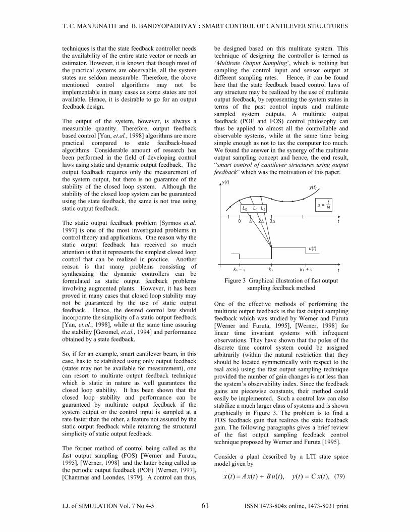
be designed based on this multirate system. This technique of designing the controller is termed as ‘Multirate Output Sampling’, which is nothing but sampling the control input and sensor output at different sampling rates. Hence, it can be found here that the state feedback based control laws of any structure may be realized by the use of multirate output feedback, by representing the system states in terms of the past control inputs and multirate sampled system outputs. A multirate output feedback (POF and FOS) control philosophy can thus be applied to almost all the controllable and observable systems, while at the same time being simple enough as not to tax the computer too much. We found the answer in the synergy of the multirate output sampling concept and hence, the end result, “smart control of cantilever structures using output feedback” which was the motivation of this paper.

y t( )

� =tN

t0 � 2� 3�

u t( )

tk +� �k�k� � �

y t( )

L0 L1 L2

Figure 3 Graphical illustration of fast output

sampling feedback method One of the effective methods of performing the multirate output feedback is the fast output sampling feedback which was studied by Werner and Furuta [Werner and Furuta, 1995], [Werner, 1998] for linear time invariant systems with infrequent observations. They have shown that the poles of the discrete time control system could be assigned arbitrarily (within the natural restriction that they should be located symmetrically with respect to the real axis) using the fast output sampling technique provided the number of gain changes is not less than the system’s observability index. Since the feedback gains are piecewise constants, their method could easily be implemented. Such a control law can also stabilize a much larger class of systems and is shown graphically in Figure 3. The problem is to find a FOS feedback gain that realizes the state feedback gain. The following paragraphs gives a brief review of the fast output sampling feedback control technique proposed by Werner and Furuta [1995]. Consider a plant described by a LTI state space model given by

),()(),()()(.

txCtytuBtxAtx =+= (79)



where nx ℜ∈ , mu ℜ∈ , py ℜ∈ , nnA ×ℜ∈ , mnB ×ℜ∈ , npC ×ℜ∈ , A , B , C , are constant

matrices of appropriate dimensions and it is assumed that the model is controllable and observable. Assume that output measurements are available at time instants τkt = , where ....,3,2,1,0=k Now, construct a discrete linear time invariant system from these output measurements at sampling rate τ/1 (sampling interval of τ secs) during which the control signal u is held constant. The system obtained so is called as the τ system and is given by

),()(

),()())1((ττ

τττ ττ

kxCkykukxkx

=Γ+Φ=+

(80)

where C,, ττ ΓΦ are constant matrices of appropriate dimensions. Assume that the plant is to be controlled by a digital computer, with sampling intervalτ and zero order hold and that a sampled data state feedback design has been carried out to find a state feedback gain F such that the closed loop system ( ) ( ) )( τττ ττ kxFkx Γ+Φ=+ (81)

has desirable properties. Let N/τ=∆ , where >N the observability index υ of the system. The

control signal u(k), which is applied during the interval ττ )1( +≤≤ ktk is then generated according to

[ ]

k

N

yLky

kyky

LLLk

=

⎥⎥⎥⎥⎥⎥

⎦

⎤

⎢⎢⎢⎢⎢⎢

⎣

⎡

∆−

∆+−−

= −

)(::

)()(

.....)( 110

τ

ττττ

u(82)

where the matrix blocks jL represent the output

feedback gains and the notation kyL , has been

introduced here for convenience. Note that τ/1 is the rate at which the loop is closed, whereas the output samples are taken at the times N - times faster rate ∆/1 . To show how a FOS controller in Eq. (82) can be designed to realize the given sampled data state feedback gain for a controllable and observable system, we construct a fictitious, lifted system for which the Eq. (82) can be interpreted as static output feedback [Syrmos et.al. 1997]. Let ( )C,,ΓΦ denote the system in Eq. (79)

sampled at the rate ∆/1 . Consider the discrete time system having at time τkt = , the input

)( τkuuk = , the state )( τkxxk = and the output

ky as

,, 0011 kkkkkk uxyuxx DC +=Γ+Φ= ++ ττ (83)

where

⎥⎥⎥⎥⎥⎥

⎦

⎤

⎢⎢⎢⎢⎢⎢

⎣

⎡

ΓΦ

Γ=

⎥⎥⎥⎥

⎦

⎤

⎢⎢⎢⎢

⎣

⎡

Φ

Φ=

∑−

=

−

2

0

0

1

0

0

,N

j

jN C

C

C

CC

MM

DC . (84)

Now, design a state feedback gain F such that ( )Fττ Γ+Φ has no eigen values at the origin and provides the desired closed loop behaviour. Then, assuming that in the interval )( τττ +≤≤ ktk , )()( τkxFtu = , (85) one can define the fictitious measurement matrix, ( )( ) 1

00),( −Γ+Φ+= FFNF ττDCC , (86) which satisfies the fictitious measurement equation kk xy C= . (87)

For L to realize the effect of F , it must satisfy the equation. F=LC . (88)

Let υ denote the observability index of ( )C,,ΓΦ . It can be shown that for υ≥N , generically C has full column rank, so that any state feedback gain can be realized by a fast output sampling gain L . If the initial state is unknown, there will be an error

kkk xFuu −=∆ in constructing the control signal under the state feedback; one can verify that the closed-loop dynamics are governed by

⎥⎦

⎤⎢⎣

⎡∆⎥

⎦

⎤⎢⎣

⎡Γ−

ΓΓ+Φ=⎥⎦

⎤⎢⎣

⎡∆ +

+

k

k

k

k

ux

FF

ux

τ

τττ

01

1

0 LD. (89)

The system in Eq. (83) is stable if F stabilizes and only if ( )ττ ΓΦ , and the matrix ( )τΓ− F0LD has all its Eigen values inside the unit circle. It is evident that the eigen values of the closed loop system under a FOS control law are those of ( )Fττ Γ+Φ together with those of

( )τΓ− F0LD . This suggests that the state

feedback F should be obtained so as to ensure the stability of both ( )Fττ Γ+Φ and ( )τΓ− F0LD . The problem with controllers obtained in this way is that, although they are stabilizing and achieve the desired closed loop behaviour in the output sampling instants, they may cause an excessive oscillation between sampling instants.



The fast output sampling feedback gains obtained may be very high. To reduce this effect, we relax the condition that L exactly satisfy the linear equation (88) and include a constraint on the gain L . Thus, we arrive at the following in Eqs. (90)-(91) as 1ρ<L 20 ρτ <Γ− FLD (90)

3ρ<− FLC (91)

where 1ρ to 3ρ represents the upper bounds on

the spectral norms of L , ( )τΓ− F0LD and

( )F−LC . This can be formulated in the form of Linear Matrix Inequalities as

,02

1 <⎥⎥⎦

⎤

⎢⎢⎣

⎡

−−

II

TLLρ

( )0

23 <

⎥⎥⎦

⎤

⎢⎢⎣

⎡

−−−−IFC

FCITL

Lρ (92)

( ),0

0

02

2 <⎥⎥⎦

⎤

⎢⎢⎣

⎡

−Γ−Γ−−

IFFI

Tτ

τρLD

LD (93)

In this form, the LMI control optimization toolbox is used for the synthesis of L [Geromel et.al., 1994], [Yan, et.al., 1998], [Gahinet, et.al., 1995]. Here, 1ρ means low noise sensitivity, 2ρ small means fast decay of observation error, and most importantly,

3ρ small means that the FOS controller with gain

L is a good approximation of the originally designed state feedback controller. If 03 =ρ , then

L is an exact solution. If suitable bounds 21 , ρρ are known, one can keep these bounds fixed and minimize 3ρ under these constraints. This requires a search for a FOS controller which gives the best approximation of the given state feedback designed under the constraints represented by 1ρ and 2ρ . It should be noted here that closed loop stability requires 12 <ρ , i.e., the eigen values which determine the error dynamics must lie within the unit disc. In this form, the function min cx( ) of the LMI control toolbox for MATLAB can be used to minimize a linear combination of 21 , ρρ and 3ρ . 4.2. Design of SISO Based FOS Controller The FEM and the state space model of the smart cantilever beam is developed in MATLAB using Timoshenko beam theory. The cantilever beam is divided into 4 finite elements and the sensor and actuator as a collocated pair are placed at finite element positions 1 or 2 or 3 or 4 respectively. A fourth order state space model of the system is obtained on retaining the first two modes of vibration of the system. Different state space models of the smart cantilever beam are obtained by

varying the sensor / actuator pair from the free end to the fixed end. The FOS control technique discussed above is used to design a controller to suppress the first 2 vibration modes of a cantilever beam through smart structure concept for the various models of the smart beam considering one sensor / actuator at a time (SISO system). Controllers are designed for the various models of the smart structure system using the developed state space models for the sensor / actuator locations at various positions along the length of the beam for the various models as given in Eq. (76) and its performance is evaluated for vibration control. Simulations are carried out in MATLAB. The first task in designing the FOS controller is the selection of the sampling interval τ . The maximum bandwidth for all the sensor / actuator locations on the beam are calculated (here, the 2nd vibratory mode of the plant) and then by using existing empirical rules for selecting the sampling interval based on bandwidth, approximately 10 times of the maximum 2nd vibration mode frequency of the system has been selected. The sampling interval used is 004.0=τ seconds. Let ( )C,, ττ ΓΦ be the discrete time systems (tau

system) of the systems in Figure 2 in Eqn. (76) sampled at a rate of τ/1 seconds respectively. It is found that the tau systems are controllable and observable. The ranks of the matrices are 4. The stabilizing state feedback gains are obtained for each of the tau systems such that the eigen values of ( )Fττ ΓΦ + lie inside the unit circle and the

response of the system has a good settling time. The impulse response of the system with the state feedback gain F is obtained. Let ( )C,,ΓΦ be the discrete time systems (delta system) of the system in Figure 2 in Eqn. (76) sampled at the rate ∆/1 secs respectively, where N/τ=∆ . The number of sub-intervals, N is chosen to be 4. An external force

extf of 1 Newton is applied for duration of 50 ms at the free end of the beam for all the 4 models of the Figure 2 and the open loop responses of the system are obtained as shown in Figures 4 to 7 respectively. Controllers based on the fast output sampling feedback control algorithm [Werner and Furuta, 1995], [Werner, 1998] has been designed to control the first 2 dominant modes of vibration of the smart cantilever beam for the 4 models of the smart beam. The fast output sampling feedback gain matrix L for the system given in Eq. (76) is obtained by solving

F≅LC using the LMI optimization method [Geromel et.al., 1994], [Yan, et.al., 1998], [Gahinet,



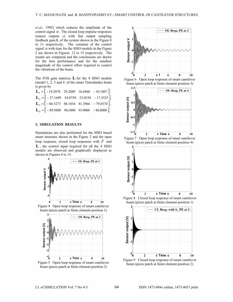
et.al., 1995] which reduces the amplitude of the control signal u . The closed loop impulse responses (sensor outputs y) with fast output sampling feedback gain L of the system shown in the Figure 8 to 11 respectively. The variation of the control signal u with time for the SISO models in the Figure 2 are shown in Figures. 12 to 15 respectively. The results are compared and the conclusions are drawn for the best performance and for the smallest magnitude of the control effort required to control the vibrations of the beam. The FOS gain matrices L for the 4 SISO models (model 1, 2, 3 and 4 of the smart Timoshenko beam is given by

[ ]1007.106960.162089.292078191 −−= .L .

[ ]5525.170538.338758.541699.372 −−=L .

[ ]0370.793966.811034.885273.863 −−=L .

[ ]8000869000911000965000894 .... −−=L . 5. SIMULATION RESULTS Simulations are also performed for the SISO based smart structure shown in the Figure 2 and the open loop response, closed loop responses with F and L , the control input required for all the 4 SISO models are observed and graphically displayed as shown in Figures 4 to 15.

Figure 4 Open loop response of smart cantilever

beam (piezo patch at finite element position 1)







Figure 8 Closed loop response of smart cantilever










Figure 12 Control effort required (piezo patch at

finite element position 1)






finite element position 4) 6. CONCLUSIONS Controllers are designed for the smart flexible cantilever beam using the FOS feedback control technique for the 4 SISO models of the smart beam to suppress the first 2 vibratory modes. The various responses are obtained for each of the SISO models. Here, the comparison and discussion of the simulation results of the vibration control for the smallest magnitude of the control effort u required to control the vibrations of the smart cantilever beam is presented. From the simulation results, it is observed that modeling a smart structure by including the sensor / actuator mass and stiffness and by varying its location on the beam from the free end to the fixed end introduces a considerable change in the system’s structural vibration characteristics. From the responses of the various SISO models, it is observed that when the piezoelectric element is placed near the clamped end, i.e., the fixed end, the sensor output voltage is greater. This is due to the heavy distribution of the bending moment near the fixed end for the fundamental mode, thus leading to a larger strain rate. The sensor voltage is very less when the sensor / actuator pair is located at the free end. The sensitivity of the sensor / actuator pair



depends on its location on the beam. From the output responses shown in the Figures 4 - 15, it is observed that the control effort u required from the controller gets reduced if the sensor / actuator placement location is moved towards the fixed end. A state feedback gain for each discrete model is obtained such that its poles are placed inside the unit circle and has a very good settling time. The individual models are compared to obtain the best performance. Comparing the 4 models, it is observed that as the smart beam is divided into 4 finite elements and the collocated pair at the fixed end, the vibration characteristics is the best. Hence, it can be concluded that, the best placement of the sensor / actuator pair is at the fixed end of the model 1. Comparing the responses of the various models of the smart beam as shown in Figure 2, model 1’s vibration response characteristics are the best for the vibration control of smart beam because of the following reasons. A small magnitude of control input u is required

to dampen out the vibrations compared to models 2, 3 and 4.

Also, the response characteristics with F and L are improved.

A state feedback gain for each of the 4 models is obtained such that its poles are placed inside the unit circle and the system has a very good settling time compared to model 2, 3 and 4.

Responses are simulated for the various models of the plant without control and is compared with the control to show the control effect. It was inferred that without control the transient response was predominant and with control, the vibrations are suppressed. The model 1 is more sensitive to the first mode as the bending moment is maximum, strain rate is higher, minimum tip deflection, better sensor output and less requirement of the control input u (control will be more effective), whereas when the piezo patch is placed at the free end of the smart beam system (model 4), because of the lesser strain rate and maximum deflection, more control effort is required to damp out the vibrations. The sensitivity to the higher modes depends not only on the collocation of the piezo pair, but also on many factors such as the gain of the amplifier used, location of the piezo pair at the nodal points and the number of finite elements. The time responses of the tip displacements for all the 4 SISO models were observed. It was seen that the tip displacement was well controlled and was within limits. Thus, an integrated finite element model to analyze the vibration suppression capability of a smart cantilever beam with surface mounted piezoelectric devices based on Timoshenko beam theory is presented in this paper. The limitations of Euler-

Bernoulli beam theory such as the neglection of the shear and axial displacements have been considered here. Timoshenko beam theory corrects the simplifying assumptions made in Euler-Bernoulli beam theory and the model obtained can be a exact one. It can be inferred from the simulation results that a FOS feedback controller applied to a smart cantilever beam model based on Timoshenko beam theory is able to satisfactorily control the modes of vibration of the smart cantilever beam. Also, the vibrations are damped out in a lesser time, which can be observed from the simulation results. Surface mounted piezoelectric sensors and actuators are usually placed at nearby the fixed end position of the structure to achieve most effective sensing and actuation. The designed FOS feedback controller requires constant gains and hence may be easier to implement in real time. REFERENCES Abramovich H., and Lishvits A., 1994, “Free

vibrations of non-symmetric cross-ply laminated composite beams,” Journal of Sound and Vibration, Vol. 176, No. 5, pp. 597 – 612.

Aldraihem O.J., Wetherhold R.C., and Singh T., 1997, “Distributed control of laminated beams : Timoshenko Vs. Euler-Bernoulli Theory,” J. of Intelligent Materials Systems and Structures, Vol. 8, pp. 149–157.

Abramovich H., 1998, “Deflection control of laminated composite beam with piezoceramic layers-Closed form solutions,” Composite Structures, Vol. 43, No. 3, pp. 217–131.

Aldraihem O.J., and Ahmed K.A., 2000, “Smart beams with extension and thickness-shear piezoelectric actuators,” Smart Materials and Structures, Vol. 9, No. 1, pp. 1–9.

Ahmed K., and Osama J.A., 2001, “Deflection analysis of beams with extension and shear piezoelectric patches using discontinuity functions” Smart Materials and Structures, Vol. 10, No. 1, pp. 212–220.

Azulay L.E., and Abramovich H., 2004, “Piezoelectric actuation and sensing mechanisms-Closed form solutions,” Composite Structures J., Vol. 64, pp. 443–453.

Baily T., and Hubbard Jr. J.E., 1985, “Distributed piezoelectric polymer active vibration control of a cantilever beam,” J. of Guidance, Control and Dynamics, Vol. 8, No.5, pp. 605–611.

Balas M.J., 1978, “Feedback control of flexible structures,” IEEE Trans. Automat. Contr., Vol. AC-23, No. 4, pp. 673-679.

Burdess J.S., and Fawcett J.N., 1992, “Experimental evaluation of piezoelectric actuator for the control of vibrations in a cantilever beam,” J. Syst. Control. Engg., Vol. 206, No. 12, pp. 99-106.



Brennan M.J., Bonito J.G., Elliot S. J., David A., and Pinnington R.J., 1999, “Experimental investigation of different actuator technologies for active vibration control,” Journal of Smart Materials and Structures, Vol. 8, pp. 145-153.

Bona B.M., Indri M., and Tornamble A., 1997, “Flexible piezoelectric structures-approximate motion equations, control algorithms,” IEEE Trans. Auto. Contr., Vol. 42, No. 1, pp. 94-101.

Benjeddou, Trindade M.A., and Ohayon R., 1999, “New shear actuated smart structure beam finite element,” AIAA J., Vol. 37, pp. 378–383.

Crawley E.F., and Luis J. De, 1987, “Use of piezoelectric actuators as elements of intelligent structures,” AIAA J., Vol. 25, pp. 1373–1385.

Chandrashekhara K., and Varadarajan S., 1997, “Adaptive shape control of composite beams with piezoelectric actuators,” J. of Intelligent Materials Systems and Structures, Vol. 8, pp. 112–124.

Culshaw B., 1992 , “Smart Structures : A concept or a reality,” J. of Systems and Control Engg., Vol. 26, No. 206, pp. 1–8.

Cooper C.R., 1966, “Shear coefficient in Timoshenko beam theory,” ASME J. of Applied Mechanics, Vol. 33, pp. 335–340.

Choi S.B., Cheong C., and Kini S., 1995, “Control of flexible structures by distributed piezo-film actuators and sensors,” J. of Intelligent Materials and Structures, Vol. 16, pp. 430–435.

Chammas B., and Leondes C.T., 1979, “Pole placement by piecewise constant output feedback,” Int. J. Contr., Vol. 29, pp. 31–38.

Doschner, and Enzmann M., 1998, “On model based controller design for smart structure,” Smart Mechanical Systems Adaptronics SAE International USA, pp. 157–166.

Donthireddy P., and Chandrashekhara K., 1996, “Modeling and shape control of composite beam with embedded piezoelectric actuators,” Comp. Structures, Vol. 35, No. 2, pp. 237–244.

Fanson J.L., and Caughey T.K., 1990, “Positive position feedback control for structures,” AIAA J., Vol. 18, No. 4, pp. 717–723.

Forouza P., 1993, “Distributed controllers for flexible structures using piezo-electric actuators / sensors,” Proc. the 32nd Conference on Decision and Control, Texas, pp. 1367-1369.

Geromel J.C., De Souza C.C., and Skeleton R.E., 1994, “LMI Numerical solution for output feedback stabilization,” Proc. American Contr. Conf., pp. 40–44.

Gosavi S.V., and Kelkar A.V., 2004, “Modeling, identification, and passivity-based robust control of piezo-actuated flexible beam,” Journal of Vibration and Acoustics, Vol. 129, pp. 260-271.

Gahinet P., Nemirovski A., Laub A.J., and Chilali M., 1995, “LMI Tool box for Matlab”, The Math works Inc., Natick MA.

Hanagud S., Obal M.W., and Callise A.J., 1992, “Optimal vibration control by the use of

piezoceramic sensors and actuators,” J. of Guidance, Control and Dyn., Vol. 15, No. 5, pp. 1199–1206.

Hwang W., and Park H.C., 1993, “Finite element modeling of piezoelectric sensors and actuators”, AIAA J., Vol. 31, No. 5, pp. 930–937.

Kosmataka J.B., and Friedman Z., 1993, “An improved two-node Timoshenko beam finite element”, Computers and Struct., Vol. 47, No. 3, pp. 473–481.

Levine W.S., and Athans M., 1970, “On the determination of the optimal constant output feedback gains for linear multivariable systems,” IEEE Trans. Auto. Contr., Vol. AC-15, pp. 44–48.

Manjunath T.C., and Bandyopadhyay B., 2006, “Multivariable control of smart Timoshenko beam structures using POF technique,” Proc. International Journal of Signal Processing, Vol. 3, No. 2, pp. 74 - 90.

Manjunath T.C. and Bandyopadhyay B., 2005, “Modeling and fast output sampling feedback control of a smart Timoshenko cantilever beam,” International Journal of Smart Structures and Systems, Vol. 1, No. 3, pp. 283-308.

Murali G., Pajunen G.A., 1995, “Model reference control of vibrations in flexible smart structures,” Proc. 34th Conference on Decision and Control, New Orleans, USA, pp. 3551-3556.

Moita J.S.M., Coreia I.F.P., Soares C.M.M., and Soares C.A.M., 2004, “Active control of adaptive laminated structures with bonded piezoelectric sensors and actuators,” Computers and Structures, Vol. 82, pp. 1349 - 1358.

Robin Scott, Michael Brown and Martin Levesley, 2003, “Robust multivariable control of a double beam cantilever smart structure,” J. of Smart Materials and Structures, Vol. 13, pp. 731-743.

Raja S., Prathap G., and Sinha P.K., 2002, “Active vibration control of composite sandwich beams with piezoelectric extension-bending and shear actuators,” Smart Materials and Structures, Vol. 11, No. 1, pp. 63–71.

Rao S., and Sunar M., 1994, “Piezoelectricity and its uses in disturbance sensing and control of flexible structures : A survey,” Applied Mechanics Rev., Vol. 47, No. 2, pp. 113–119.

Sun C.T., and Zhang X.D., 1995, “Use of thickness-shear mode in adaptive sandwich structures,” Smart Materials and Structures J., Vol. 3, No. 4, pp. 202–206.

Syrmos V.L., Abdallah P., Dorato P., and Grigoriadis K., 1997, “Static output feedback : A survey,” Automatica, Vol. 33, No. 2, pp. 125–137.

Schiehlen W., and Schonerstedt H., 1998, “Controller design for the active vibration damping of beam structure,” Smart Mechanical Systems Adaptronics SAE International, USA, pp. 137-146.



Seshu P., 2004, “Textbook of Finite Element Analysis,” 1st Ed. Prentice Hall of India, New Delhi.

Shiang Lee W., 1996, “System identification and control of smart structures using neural networks,” Automatica, Vol. 38, No. 4-8, pp. 269-276.

Thomas J., and Abbas B.A.H., 1975, “Finite Element Methods for dynamic analysis of Timoshenko beam,” J. of Sound and Vibration, Vol. 41, pp. 291–299.

Tokhi M.O., 1994, “Self tuning active vibration control in flexible beam structures,” Journal of Systems and Control Engineering - Proceedings of the Institute of Mechanical Engineers, Vol. 208, pp. 263-277.

Werner H., 1997, “Robust multivariable control of a turbo-generator by periodic output feedback,” Vol. 31, No. 4, pp. 395 - 411.

Umapathy M., and Bandyopadhyay B., 2000, “Vibration control of flexible beam through smart structure concept using periodic output feedback,” System Science Journal, Vol. 26, No. 1, pp.23 - 46.

Umapathy M., and Bandyopadhyay B., 2002, “Design of fast output sampling feedback control for smart structure model,” Proc. of SPIE 9th Annual Symposium / Conference on Smart Structures and Materials / NDE Joint Conference, San Diego, CA, USA, Vol. 4693, pp. 222-233.

Ulrich Gabbert1, Tamara Nestorović Trajkov1, and Heinz Köppel, 2002, “Modeling, control, simulation of piezoelectric smart structures using FEM and optimal LQ control,” Facta Universitatis Series: Mechanics, Auto. Control and Robotics, Vol. 3, No 12, pp. 417 - 430.

Vukovich G., and Koma A.Y., 2000, “Vibration suppression of flexible beams with bonded piezo-transducers using wave-absorbing controllers,” J. Guidance, Control and Dynamics, pp. 347-354.

Werner H., and Furuta K., 1995, “Simultaneous stabilization based on output measurements,” Kybernetika, Vol. 31, No. 4, pp. 395–411.

Werner H., 1998, “Multimodal robust control by fast output sampling-An LMI approach,” Automatica, Vol. 34, No. 12, pp. 1625-1630.

Young-Hun Lim, Senthil Gopinathan V., Vasundara Varadhan V., and Vijay Varadan K., 1999, “Finite element simulation of smart structures using an optimal output feedback controller for vibration and noise control,” Journal of Smart Materials and Structures, Vol. 8, pp. 324-337.

Yang S.M., and Lee Y.J., 1993, “Optimization of non-collocated sensor / actuator location and feedback gain in control systems,” Journal of Smart Materials Structures, Vol. 8, pp. 96-102.

Yan Y.C., Lam J., and Sun Y.X., 1998, “Static output feedback stabilization: An LMI approach,” Automatica, Vol. 34, No. 12, pp. 1641–1645.

Zhang X.D., and Sun C.T., 1996, “Formulation of an adaptive sandwich beam,” Smart Mater. and Struct., Vol. 5, No.6, pp. 814–823.

BIOGRAPHIES

T. C. Manjunath, born in Bangalore, Karnataka, India on Feb. 6, 1967 received the B.E. Degree in Electrical Engineering from the University of Bangalore in 1989 in First Class and M.E. in Automation and Control

Engineering with specialization in Automation, Control and Robotics from the University of Gujarat in 1995 in First Class with Distinction, respectively. He has got a teaching experience of 17 long years in various engineering colleges all over the country and is currently a Research Scholar doing Ph.D. in the Department of Systems and Control Engineering, Indian Institute of Technology Bombay, India in the field of modeling, simulation, control and implementation of smart flexible structures using DSpace and its applications.

B. Bandyopadhyay, born in Birbhum village, West Bengal, India, on 23rd August 1956 received his Bachelor's degree in Electronics and Communication Engineering from the University of Calcutta, Calcutta, India, and

Ph.D. in Electrical Engineering from the Indian Institute of Technology, Delhi, India in 1978 and 1986, respectively. In 1987, he joined the Interdisciplinary Programme in Systems and Control Engineering, Indian Institute of Technology Bombay, India, as a faculty member, where he is currently a Professor.

Date post:	09-Jun-2018
Category:	Documents
Upload:	vunhan
View:	220 times
Download:	0 times

SMART CONTROL OF CANTILEVER STRUCTURES …ijssst.info/Vol-07/No-4-5/Paper7.pdf · as they may...

Documents