36
Smart Metering Early Learning Project: Domestic Energy Consumption Analysis Report and Technical Annex [March 2015]
Smart Metering Early Learning Project:
Domestic Energy Consumption Analysis
Report and Technical Annex
[March 2015]

2
© Crown copyright [2015]
URN [15D/081]
You may re-use this information (not including logos) free of charge in any format or medium, under the terms of the Open Government Licence.
To view this licence, visit www.nationalarchives.gov.uk/doc/open-government-licence/ or write to the Information Policy Team, The National Archives, Kew, London TW9 4DU, or email: [email protected].
Any enquiries regarding this publication should be sent to us at [[email protected]].

3
Contents
Contents .................................................................................................................................... 3
1. Executive summary ............................................................................................................. 5
2. Introduction ........................................................................................................................ 7
2.1 Background ..................................................................................................................... 7
2.2 The Early Learning Project (ELP) ..................................................................................... 8
2.3 Aims of the Energy Consumption Analysis Project ....................................................... 8
2.4 Project Design and Method Development .................................................................... 9
3. Data Sources .................................................................................................................... 11
3.1 Energy Supplier Data .................................................................................................... 11
3.2 Elexon Load Profiling Data ........................................................................................... 11
3.3 Degree-day Data .......................................................................................................... 12
3.4 Experian Data ................................................................................................................ 12
4. Methodology .................................................................................................................... 13
4.1 Methodology Overview ................................................................................................ 13
4.2 Creating the Control Group ......................................................................................... 13
5. Implementing the Method ............................................................................................... 14
5.1 Project Steps ................................................................................................................. 14
5.2 Producing a Timeline of Energy Consumption ............................................................ 15
5.3 Controlling for Seasonal Effects ................................................................................... 15
5.4 Exclusion Criteria ........................................................................................................... 16
5.5 Stratifying the Control Group ....................................................................................... 17
5.6 Comparing Treatment and Control Group Distributions ............................................. 17
5.7 Sample Sizes ................................................................................................................. 18
6. Results .............................................................................................................................. 19
6.1 Findings ......................................................................................................................... 19
7. Discussion of Results ........................................................................................................ 20
7.1 Assumptions of the Analysis ........................................................................................ 20
7.2 Data Limitations ............................................................................................................ 21
8. Conclusions ...................................................................................................................... 22
8.1 Conclusions ................................................................................................................... 22

4
8.2 Recommendations for Future Research ....................................................................... 23
Annexes ................................................................................................................................... 25
Glossary of Terms .................................................................................................................... 34

5
1. Executive summary
The Energy Consumption Analysis Project is one of a number of research studies that form part of the Early Learning Project, with the overall aim of exploring the experiences and benefits of domestic consumers in the early stages of the Smart Metering Implementation Programme, prior to installation of meters at scale.
The aims of the Domestic Energy Consumption Analysis project were to develop and implement a robust methodology to quantify the impact of early smart-type meters on household energy consumption; and to feed in information on the early levels of energy saving to other elements of the Early Learning Project.
The first aim was achieved by adopting a difference-in-difference design that compared annual energy consumption levels between a treatment group (who received a smart-type meter) and a control group (who did not). The extent to which energy consumption within the treatment group fell by more than that of the control group provides an estimate of the impact of the installation of smart-type meters during this period.
Using a difference-in-difference analysis, the results showed that for electricity, smart-type meters enabled an average annual reduction compared to traditional meters of 2.3 per cent with 95 per cent confidence intervals between 1.6 per cent and 2.8 per cent, and for gas, an average annual reduction compared to traditional meters of 1.5 per cent with 95 per cent confidence intervals of 0.9 per cent and 2.1 per cent. These findings are statistically significant and provide evidence that smart-type meters installed during 2011 enabled energy saving benefits to be realised during this early stage in the Programme’s development.
This research report is one of five which have been published concurrently[1], containing the findings of DECC’s programme of ‘early learning’ smart meter research and small-scale trials. This was based on research with early recipients of smart and smart-type meters. It was aimed at extending the Government’s and stakeholders’ understanding of how best to deliver consumer benefits, and providing evidence from which to assess the need for any changes to the policy and regulatory framework.
A further Policy Conclusions report summarises DECC’s view of the key findings, and sets them in the context of further progress, since the research was conducted, to establish the delivery framework for smart metering. This report also provides the Government’s conclusions about future consumer engagement policy and delivery priorities, and the steps to implement them, working with Ofgem, Smart Energy GB, suppliers and other parties.
[1] https://www.gov.uk/government/publications/smart-metering-early-learning-project-and-small-scale-behaviour-
trials

6

7
2. Introduction
This section introduces the Smart Metering Implementation Programme (SMIP), outlines the aims and objectives of the Domestic Energy Consumption Analysis project and sets the work in the context of the broader Early Learning Project.
2.1 Background
Smart meters are the next generation of gas and electricity meters offering a range of intelligent functions. The Government’s vision is for every home and smaller business in Great Britain to have their existing meters replaced by smart electricity and gas meters by the end of 2020. The roll-out of smart meters will play an important role in Britain’s transition to a low carbon economy and help meet some of the long-term challenges faced in ensuring an affordable, secure and sustainable energy supply.
Smart meters are expected to deliver a range of benefits to consumers, which include bringing an end to estimated billing and providing consumers with near real- time information on their energy consumption through the use of an In-Home Display unit (IHD1) supplied with the smart meter. It is envisaged that this will provide consumers with better control over their energy use, help them to budget better and help make switching between suppliers smoother and faster.
The Smart Metering Implementation Programme is currently in Foundation Stage, which began in March 2011. The Government is working with the energy industry, consumer groups and other stakeholders to put commercial and regulatory frameworks in place to support smart metering, trial and test systems, learn lessons from early installations and enhance the consumer experience. Most householders will then have smart meters installed by their energy supplier during the Programme’s Main Installation Stage.
The definition of a ‘smart meter’ is one that is compliant with the Smart Meter Equipment Technical Specification (SMETS2) and has functionality such as being able to transmit meter readings to suppliers and receive data remotely. ‘Smart-type’ meters offer some of the functionality of SMETS and have been used to facilitate
early operational development for some suppliers as well as providing their
1 IHD’s allows consumers to see what energy they are using and how much it is costing in near real-
time, including information about the amount of energy used in the past day, week, month and year.
2 https://www.gov.uk/government/uploads/system/uploads/attachment_data/file/43087/6425-smart-
metering-equipment-technical-specifications-.pdf

8
customers with early access to some of the benefits of smart metering. This report uses data collected from ‘smart-type’ meters installed during 2011 and explores potential consumer benefits of these early recipients. Smart-type meters installed in domestic properties will need to be replaced with SMETS compliant smart meters by the end of 2020 in accordance with supplier roll-out obligations (see Annex 1 for meter definitions).
2.2 The Early Learning Project (ELP)
The Department for Energy and Climate Changes (DECC) initiated the Early Learning Project (ELP) in the second half of 2012, to explore the experiences of domestic consumers involved in the early part of the Foundation Stage and to investigate the outcomes they experienced. It fulfils a commitment in the Monitoring and Evaluation Strategy for smart metering3 to assess consumer benefits from smart metering at an early stage, in order to help assess whether suppliers’ engagement plans are likely to be sufficient to deliver the Programme objectives, and to inform subsequent policy decisions. Another objective of the project is to test and refine the methodology to ensure there is a robust approach to evaluating the Programme’s Main Installation Stage.
2.3 Aims of the Energy Consumption Analysis Project
The Government has undertaken to design and implement a framework for monitoring and evaluating the impacts of the Smart Meter Implementation Programme. This will enable Government to report on progress and the delivery of consumer and other benefits. Measuring consumer energy saving is an important part of our monitoring and evaluation activity.
There were two main aims of the Domestic Energy Consumption Analysis project. One was to develop a robust methodology to evaluate the impact of smart-type meters on household energy consumption. This aim included learning from the practical experience of collecting data from energy suppliers and administrative sources, and the processing, analysing and interpretation of smart-type meter energy consumption data. It is envisaged that this work will form the methodological foundations from which to develop a long term strategy for measuring consumer benefits during the Main Installation Stage of the Programme.
The other aim was to feed in information on the early levels of energy saving to other elements of the Early Learning Project. In particular, these results inform the synthesis project, which aims to build an overall analysis of requirements for
consumer engagement to optimise energy saving benefits, based on learning from the early Foundation Stage of the Programme and wider evidence.
3 https://www.gov.uk/government/uploads/system/uploads/attachment_data/file/43119/5454-strategy-
cons-smart-meters-monitor-eval.pdf
9
2.4 Project Design and Method Development
To develop a robust methodology for evaluating domestic energy consumption changes associated with the introduction of smart meters in Great Britain, identifying both a suitable design for the evaluation and data that could be used to implement it was necessary.
Design of the evaluation and data requirements was informed by a preparatory phase of work to develop the Programme’s overall evaluation strategy for monitoring consumer impacts, and to ensure that the Programme aligns with commitments published in the Monitoring and Evaluation Strategy (referenced in Section 2.2).
Preparation began in July 2011. This included a workshop with suppliers and stakeholders under the heading ‘Preparing for Evaluation4’, which considered general issues about evaluation design and implementation, as well as emerging
evidence from early smart-type meter trials through the Energy Demand Research Project5,6 that had just been published. The Energy Demand Research Project (EDRP) was a major set of trials, designed to help better understand how domestic consumers react to improved information about their energy consumption over the long term.
High level messages from this workshop included the importance of effective communication about the evaluation with suppliers so that they understand what is planned; and the need for DECC to plan the evaluation comprehensively in terms of what questions will be addressed and the data required.
Initial consideration was given to the possibility of using an experimental approach, e.g. using a randomised control trial (RCT) to randomly allocate a sample of households into two groups: an intervention group who then have a smart-type meter installed and a control group who do not. However this was rejected for two reasons. Firstly there would be practical difficulties in implementing such a design; and secondly, challenges due to the nature of the intervention.
On the first point, the smart meter roll-out is supplier-led (individual energy suppliers are responsible for deciding when consumers will be offered smart meters during the Main Installation Stage). It would therefore be difficult to pre-select groups of consumers who would, and would not, receive smart meters at specific dates for the purposes of evaluation.
On the second point, the element of consumer choice (whether consumers agree to have a smart meter installed) would make it difficult to conduct the evaluation as an experimental trial involving randomised assignment of consumers. While there are modified approaches such as ‘waiting list’ trials that involve recruiting a pool of
consumers and then assigning them randomly to intervention and control groups,
4 Smart meter evaluation: consumer benefits workshop report - Published September 2011
5 Smart meter evaluation: lessons from EDRP - Published August 2011
6 https://www.ofgem.gov.uk/ofgem-publications/59105/energy-demand-research-project-final-
analysis.pdf

10
recruitment itself is an intervention that is likely to affect energy consumption behaviour.
Another part of the preparation for consumer impact evaluation was the Smart Meters Evaluation Data Framework (Consumer Impacts) (SMED) project carried out for DECC by AECOM and UCL between Autumn 2011 and June 2012. The project’s aim was to identify indicators and existing data sources, highlight gaps where primary data collection may be required, and data collection methods for consumer impact evaluation. The SMED project informed the design of the Early Learning Project, including both the consumer experience survey and energy consumption analysis. In particular, SMED recommended (i) the adoption of a quasi-experimental methodology for evaluating energy consumption impacts of smart meters and (ii) the need for additional primary data from energy suppliers.
These preparatory investigations informed the design phase of the domestic energy consumption evaluation, on which DECC received further independent advice from the Office for National Statistics Methodology Advisory Service in the autumn of 2012. The Programme also engaged in bilateral discussions with two energy suppliers who had been early installers of smart-type meters, discussing the necessary data requirements and agreeing plans to carry out the analysis. A quasi-experimental design employing a ‘difference-in-difference’ methodology was recommended in the SMED report, as a means of dealing with the inherent variability of energy consumption over time (due to weather effects, energy prices and other external factors).
Evidence from these research findings helped inform the analysis and recommendations produced for DECC by the Office for National Statistics (ONS). A ‘difference-in-difference’ approach was confirmed as appropriate to this study, whereby change in the variable of interest (energy consumption) should be measured by comparing the difference in consumption change over a given period of time between an intervention group and a matched comparison group (established on the basis of relevant stratification variables).

11
3. Data Sources
The difference-in-difference analysis conducted for the Energy Consumption project required the manipulation of large data-sets containing domestic gas and electricity meter- and read-level data from suppliers. It also required Elexon Load Profiling and Degree-day data for extrapolation purposes, and Experian data to provide variables for stratification. These data sources are further discussed below and a process flow diagram illustrating when these data sources are incorporated in the analysis can be found in Annex 2.
3.1 Energy Supplier Data
As part of the SMED project, an assessment of data held within DECC concluded that data required for this project would need to be provided directly from energy suppliers. The Department approached two suppliers who had been early installers of smart-type meters to discuss the scope of the project and data required for analysis. This then formed the content of an information request as part of suppliers’ licence conditions. A data specification table outlining variables required for analysis can be found in Annex 3.
Key to the project was the provision of meter- and read-level data from energy suppliers. The data provided by each supplier contained an MPAN/MPRN (Meter-Point Administration/Reference Number) as a unique identifier, a flag and date indicating if and when a smart meter had been installed, and individual meter reads and read dates for the period of January 2010 to December 2012.
The structure of the data provided by suppliers for electricity and gas was very similar. The only difference was that all electricity reads were provided in kWhs (kilowatt hours) whereas gas data was received in a mix of kilowatt hours (kWh), cubic metres (m3) and hundreds of cubic feet (HCF). A variable was provided to indicate which of these units applied to which meter. A process of conversion was applied to standardise the measure to kWhs. This is described in Annex 4.
3.2 Elexon Load Profiling Data
An Electricity Load Profile represents the pattern of electricity usage by day and by year for the average domestic customer. For this project, Elexon Load Profiling data was used to extrapolate consumption from the nearest actual read available in the data to the date one year before and one year after installation. These two dates from herein are referred to as ‘t-1’ and ‘t+1’ (where ‘t’ represents the date of installation of a smart meter). More information on how Elexon Load Profiling was

12
employed in the project is discussed in Section 5.2 and Annex 5. More general information on Elexon Load Profiling can be found on their website7.
3.3 Degree-day Data
Degree-day data supplied by the UK Met Office was employed to extrapolate gas consumption. Most gas in the home is consumed for heating purposes and heating energy consumption depends largely on external (weather-related) temperatures. A degree-day is based on a composite weather variable applied to each day where the outside temperature falls below a base temperature. The base temperature is defined as the outside temperature above which the heating system in a building would not be required to operate. Published degree days in the UK are calculated to a base temperature of 15.5ºC for general use. Therefore any temperature below
15.5ºC would generate a degree-day coefficient for that particular day. For instance, 12.5oC would produce a coefficient of 3 as it is 3 degrees below the base temperature. The analysis selected a weather station in each Government Office Region and matched the location of each meter to the appropriate weather station degree-day data. This allowed us to apportion the correct amount of gas that would be consumed for any given day where there is not actual data. Further discussion on this can be found in Annex 5. More information on degree-day data can be found through Eurostat8.
3.4 Experian Data
The project obtained modelled household data from Experian9, which was linked to individual meters to provide a proxy for property and household characteristics. These characteristics were then used as additional stratifiers during the matching process (between control and treatment groups) to control for extraneous factors that may affect energy consumption levels. More detailed information on Experian variables employed can be found in Section 5.5 and Annex 6.
7 http://www.elexon.co.uk/reference/technical-operations/profiling/
8 http://epp.eurostat.ec.europa.eu/cache/ITY_SDDS/en/nrg_esdgr_esms.htm
13
4. Methodology
4.1 Methodology Overview
As described in Section 2, the method adopted for the project was a quasi-experimental design; specifically, a difference-in-difference approach. This approach is based on comparing changes in energy consumption over time for a ‘treatment’ and ‘control’ group of households. The treatment group was purposefully drawn from a sampling frame of households that had smart-type meters installed in 2011 only (the earlier part of the Programme’s Foundation Stage), while the control group consisted of households with similar characteristics (that had been matched) to the
treatment group but where no smart-type meter had been installed (as discussed below).
4.2 Creating the Control Group
The method employed four different ways of controlling for attributes and behaviours which may otherwise cause variation in consumption between the control and treatment groups.
Firstly, annual pre-installation consumption for smart-type and traditional meters was matched using 10 consumption bands (see Annex 6) to ensure that there was a very similar pre-installation consumption distribution across both treatment and control groups.
Second, the selection of ‘control’ households was matched on several variables to ‘treatment’ households so that, with respect to these selection variables, the comparison was like-with-like. In conjunction with consumption bands, these variables are used to stratify the control sample. The total array of stratifying variables (see Annex 6 for detailed breakdown) included;
annual pre-installation consumption band
aggregated regional geography (e.g. Scotland, North England,
Midlands, South of England)
energy supplier
residence type (e.g. Detached)
property size (Number of Bedrooms)
property age
household gross-income band.
Suppliers did not provide data on household characteristics. For the last four of these stratifying variables, meter-level data was matched via a Unique Property Reference Number (UPRN) to modelled Experian data to provide a proxy for household characteristics.

14
Thirdly, pre- and post-installation periods of energy consumption are the same between control and treatment households i.e. the installation month (and therefore annual pre- and post-installation period) for each smart-type meter is paired with that of a traditional meter. As meters in the control group do not have a comparison installation, an actual traditional meter read was attributed as a ‘dummy’ installation date from the same month. This has the impact of negating seasonal variation between the two groups.
Finally, the difference-in-difference calculation ensures that any residual differences in energy consumption between the control and treatment groups, whether systematically caused by factors which have not otherwise been controlled for, or by random variation between the two groups of households, is taken into account.
5. Implementing the Method
5.1 Project Steps
In order to implement this design, the analysis method passed through several steps (more detail can be found in the process diagram in Annex 2):
i. Deriving annual consumption figures for the year leading up to the installation
and year after installation of a smart-type meter.
ii. Allocation of a ‘dummy installation date’ for traditional meters in the control group
followed by the production of annual consumption figures.
iii. The removal of meters which did not meet the criteria.
iv. Attributing household characteristics variables to the data in the treatment and
control group.
v. Stratifying the control group so that the composition of the control sample in
terms of characteristics was the same as the treatment group.
vi. Comparing pre-installation distributions to ensure they were very similar in both
groups.
vii. Calculating the post-installation energy consumption difference between the two
groups.
These steps are discussed in more detail below.

15
5.2 Producing a Timeline of Energy Consumption
The analysis produced an annual time-line of pre- and post-installation consumption at meter level for both electricity and gas meters. Consumption figures are based on actual read data for each meter provided by suppliers. Annual pre-installation consumption figures therefore relate to the period ‘t-1’ to ‘t’, and similarly, post-installation annual consumption figures relate to the period ‘t’ to ‘t+1’ as illustrated in Figure 2.
Figure 2: Actual Meter Level Timeline
As actual reads rarely occur exactly one year before or after the installation date, the analysis selected the nearest actual read to ‘t-1’ for annual pre-installation consumption, (and similarly) ‘t+1’ for post-installation consumption. A small amount of extrapolation using Elexon Load Profiling for electricity meters and Degree-day data for gas meters was applied where necessary (see Sections 3.2, 3.3 and Annex 5 for further details on these data sources).
5.3 Controlling for Seasonal Effects
To negate any seasonal effect, it was important that the consumption of any given
smart-type meter was paired with a traditional meter in the control group over the same time period (e.g. month). As the control group consisted of meters where no smart-type meter installation had taken place, an actual read was randomly selected in 2011 to act as a ‘dummy’ installation date. The process in the previous paragraph was then implemented to produce pre- and post-installation annual consumption figures for meters in the control group. Later in the process, the installation months from both groups were paired.

16
5.4 Exclusion Criteria
Following the derivation of annual consumption figures for every meter, some meters were removed from the analysis based on the following exclusion criteria:
As there were no smart-type Economy 7 meters, all Economy 7 meters
were removed from the control group.
As there were no pre-payment meter (PPM) customers in the smart
meter group, PPM customers were removed from the control group
prior to matching.
Meters that did not have at least a year of post-installation reads were
removed as there would not be a long enough period to evaluate the
before and after effects of smart meter installations (and comparative
traditional meters) throughout all four seasons.
The method compared actual consumption reads between the two
groups. For greater accuracy, all estimated reads were removed.
The method ensured that the level of consumption extrapolation was
minimised. Meters in which there was no actual read within 90 days of
the ‘t-1’ and ‘t+1’ were removed.
Post-calculation analysis found that outliers (such as very high and low
consumption households) had an impact on results, and as the scope
of the project related to domestic properties, meters where annual
consumption were less than 1,000 kWh and greater than 12,000 kWh
for electricity meters, and less than 1,000 kWh and greater than 40,000
kWh for gas meters, were removed from both groups10.
Meters where the annual post-installation consumption was greater
than double or less than half of the annual pre-installation consumption
were removed, as these changes were deemed to be due to factors
outside of the smart meter intervention.
Meters that could not be allocated a geographic location through
matching were removed.
Match rates are presented in Annex 8.
10
Initial analysis was conducted on meters with annual consumption between 100kWH and
25,000kWh for electricity and 100kWh and 50,000kWh for gas. However, small sample sizes in the
tails of the distribution led to high variability in the estimates, and were therefore reduced to minimise
the impact.

17
5.5 Stratifying the Control Group
The method needed to control, as best as possible, for extraneous factors that were likely to have an effect on energy consumption change. To achieve this, each meter was matched to household variables using Experian data. These variables were;
residence type
property size
property age
household gross-income band.
In addition, other variables were derived that would form the total complement of variables used for the stratification process. These variables were;
pre-installation consumption band (see Annex 6)
the month of installation
energy supplier
geographic location.
Each meter in the treatment and control group therefore had valid values for all 8 of these appended variables. These were used for the stratification process (a full list of values can be found in Annex 6). The analysis then created an 8 to 10 digit code, which was a concatenation of valid values from each variable. For instance consumption band 1, installation date month 4, supplier 2, geographic location 4, residence type 2, property size 3, property age 3, income band 7, would give a code of 14242337. With each meter in both the treatment and control group having a code, we could then match meters from each group so that there was a control consisting of meters from households with the same characteristics as the treatment group. Where there were more meters in the control group than the treatment group with the same code, the traditional meter with the nearest pre-installation annual consumption was selected.
5.6 Comparing Treatment and Control Group Distributions
To ensure that that there were no significant biases between the stratified matched sample of treatment and control groups, Mann-Whitney U-statistics11 were run to
confirm (with 95 per cent confidence) that the average consumption of the control group before the installation period was the same as the equivalent treatment group. The result of the stratification process produced almost identical pre-installation consumption distributions for both the electricity sample (p=0.848) and the gas
11 Non-parametric tests were used rather than a two sample t-tests because consumption data is
positively skewed.

18
sample (p=0.978). This provided evidence that the stratification and timing variables (Degree-day and Elexon profiles) had been effective in removing sources of variation in energy consumption between the two groups, and provides a good like-for-like comparison.
As the average consumption distributions of pre-installation groups were similar, a difference-in-differences calculation was applied to test whether there had been any post-installation effect.
The pre- and post-installation annual consumption of each sample is compared and the extent to which energy consumption within the treatment group had fallen by more than that of the control group provides an estimated percentage change of the impact of the installation of smart meters. The calculation is given in the following equation:
Ratio = Σ (Annual post-installation consumption smart-type meters) /
Σ (Annual pre-installation consumption smart-type meters)
Σ (Annual post-installation consumption traditional meters) /
Σ (Annual pre-installation consumption traditional meters)
A standard transformation from ratio to percentage change is then applied (i.e. 1 minus the ratio, multiplied by 100).
5.7 Sample Sizes
Energy consumption reduction estimates are based on a stratified sample of meters. The sample sizes for this analysis was 6,070 for electricity estimates and 5,145 for gas estimates. The sample size for both electricity and gas was affected by three main factors:
The number of actual smart-type meter installations during 2011.
The number of meters in the data that contained a meter read within 90
days of ‘t-1 and ‘t+1’.
The number of smart-type meters that could be successfully matched
to a traditional meter (i.e. where a traditional meter contains the same
values in all stratifying variables).

19
6. Results
Annual energy consumption from the treatment and control groups was compared, and the extent to which energy consumption within the treatment group has fallen by more than that of the control group provided an estimate of the impact of the installation of smart-type meters. Electricity and gas meters were analysed separately.
As the analysis employed a sampling approach, 95 per cent confidence intervals were derived to demonstrate the robustness of the consumption change estimates. Confidence intervals are influenced by the size of the sample analysed and the variation of the distribution of results. Annex 7 provides detail on how these
confidence intervals were derived.
6.1 Findings
Energy consumption reduction results are based on the comparison of matched pairs of smart-type and traditional meters (n = 6,070 for electricity and n = 5,145 for gas). As illustrated in Figure 3, for electricity, smart-type meters enabled an average annual reduction of 2.3 per cent with 95 per cent confidence intervals of 1.6 per cent and 2.8 per cent over traditional meters. For gas, smart-type meters provided an average annual reduction of 1.5 per cent with 95 per cent confidence intervals of 0.9 per cent and 2.1 per cent over traditional meters.
Mann-Whitney U-statistics were also run post-installation to ascertain whether any differences in average energy consumption between the treatment and control groups were significant. The average reduction in energy consumption for both electricity and gas is statistically significant (p<0.01). This provides evidence that on average, we are seeing a statistically significant reduction in energy consumption after the installation of a smart-type meter during 2011, and that this is not just happening by chance.

20
*Statistically significant (p<0.05) reduction in annual consumption after installation of a smart-type meter
Figure 3: Impact of Smart-Type Meters on Energy Consumption Reduction
7. Discussion of Results
The Energy Consumption Analysis project has undergone a rigorous development and implementation process, engaging in internal and external review to ensure that the approach is methodologically robust. However, as with all pilot work, limitations have been identified, some of which require further investigation and are discussed below.
7.1 Assumptions of the Analysis
The project adopted a difference-in-difference methodology as presented in Section 4, and is based on the assumption that any residual differences in energy consumption between the control and treatment groups, caused by confounding factors (which have not been controlled for), are negated. However, through
2.3% 1.5%
0.0%
1.0%
2.0%
3.0%
4.0%
Electricity (n = 6,070) Gas (n = 5,145)
Per
cen
tage
Red
uct
ion
Supplier
*
*
upper95 = 2.8%
lower95 = 1.6%
upper95 = 2.1%
lower95 = 0.9%
21
implementing this work, several potential confounding variables have been identified and their assumptions listed below (although this is not necessarily a complete list):
Changes in the level of occupancy (and non-occupancy) between pre-
installation and post-installation periods are comparable in the
treatment and control groups.
Changes in household structure (arrival of children / teenagers leaving
for university / change of tenants) between pre-installation and post-
installation periods are comparable in the treatment and control groups.
The distribution of inherent error in modelled Experian data, used to
categorise households into stratifiers, occurs equally in both groups.
Differences in temperature from weather stations which form degree-
day calculations and the actual temperature at meter locations contain
equal error in both groups. An example of this might be a weather
station in the centre of a region (say the North East) where there are
houses at a coastal location in that region which may experience
slightly different temperatures.
7.2 Data Limitations
To ensure the method adopted was as robust as possible, given the data provided, a proportion of the initial pool of smart-type meters were eliminated from the sample when they failed to meet the analysis criteria (see Section 5.4). The largest proportion of this eliminated group was due to the absence of actual reads within the period of observation for this study (particularly within 90 days of t-1 and t+1). This was in part due to the large quantity of estimated reads in the pre-installation year.
To estimate the impact of a smart meter intervention, a minimum of two years consumption data is required (t-1 to t+1). As this study was carried out during the early Foundation Stage of the Programme, the research was limited by the sample size available (smart-type meter installation in 2011 only). Statistical power (0.8) and precision (0.05) for the reported analysis was achieved based on sample sizes of 6,070 and 5,145, but to enable any further analysis (such as distributional effects), a much larger sample would be required to maintain these levels of power and precision and ensure unbiased inference in the findings.
As reported in Section 5, the matching process used to derive the final sample of control and treatment groups resulted in very similar mean energy consumption pre- smart-type meter installation. These matching variables were chosen as they were readily available for use and relevant in the study context. However some of the stratifying variables used in this analysis are derived from modelled (estimated) Experian data, which carry an element of statistical uncertainty that we cannot control for. Other administrative and survey data sources are available as identified

22
in the SMED project12, and should be explored as an alternative to Experian data. There are also a number of additional variables suggested that should be considered for controlling variation in household energy consumption (such as socio-demographic information). We are considering extending this work to explore the distribution of smart meter energy saving benefits, but to enable this, a full analysis of relevant stratifying variables will need to be conducted.
As highlighted in the assumptions, using the data provided for this study, it was not possible to identify and exclude the following households during the analysis period; households that changed ownership, vacation periods in either the pre or post-year years but not both13 and structural changes to the building (i.e. extensions), especially if these unknown changes occurred during a period that is estimated using extrapolation. As we could not control for or eliminate these variables during the study, this is likely to have increased the variance in the estimates. Potential confounding variables are an area for further exploration / refinement when obtaining and processing future energy consumption data.
8. Conclusions
8.1 Conclusions
One aim of this research was to develop a robust methodology to quantify the impact of smart-type meters on household energy consumption. The project has successfully met this aim and has provided evidence that, on average, we are seeing a statistically significant reduction in energy consumption for smart-type meters installed in 2011 compared to traditional meters. The project has also contributed evidence to other elements of the Early Learning Project about how smart-type metering has enabled energy saving benefits to be realised at this early stage in the Programme’s development, meeting the second aim of the project.
The energy consumption analysis described in this report relates to smart-type meters installed in 2011 during the early Foundation Stage of the Programme. The impacts on energy consumption observed, reflect the commercial approach of
12 e.g. Homes Energy Efficiency Database (HEED), Valuation Office Agency (VOA) data, Energy
Performance Certificate (EPC), English Housing Survey (EHS), Family Expenditure Survey (FES),
British Household Panel Survey (BHPS) and others.
13 where there was a long period of non-occupancy in either the pre or post intervention year, records
could be identified and removed (cut-off point - less than 1,000 kWh of energy consumed in one of the
two time periods).
23
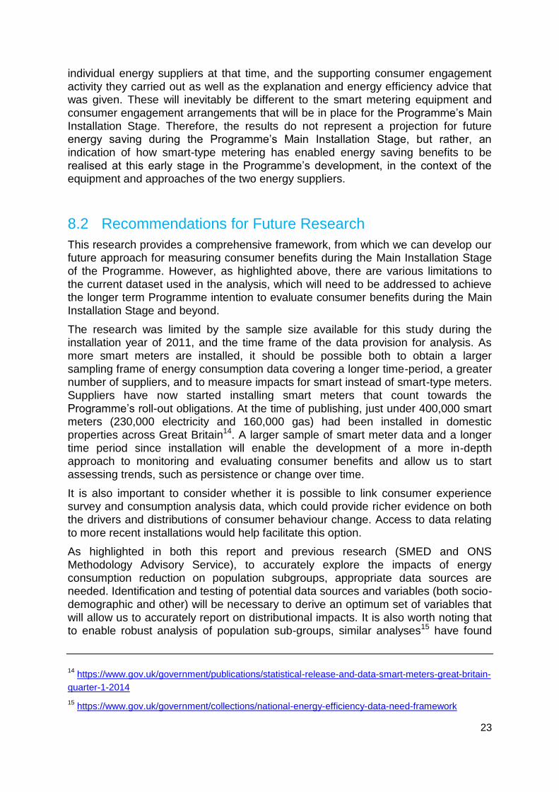
individual energy suppliers at that time, and the supporting consumer engagement activity they carried out as well as the explanation and energy efficiency advice that was given. These will inevitably be different to the smart metering equipment and consumer engagement arrangements that will be in place for the Programme’s Main Installation Stage. Therefore, the results do not represent a projection for future energy saving during the Programme’s Main Installation Stage, but rather, an indication of how smart-type metering has enabled energy saving benefits to be realised at this early stage in the Programme’s development, in the context of the equipment and approaches of the two energy suppliers.
8.2 Recommendations for Future Research
This research provides a comprehensive framework, from which we can develop our future approach for measuring consumer benefits during the Main Installation Stage
of the Programme. However, as highlighted above, there are various limitations to the current dataset used in the analysis, which will need to be addressed to achieve the longer term Programme intention to evaluate consumer benefits during the Main Installation Stage and beyond.
The research was limited by the sample size available for this study during the installation year of 2011, and the time frame of the data provision for analysis. As more smart meters are installed, it should be possible both to obtain a larger sampling frame of energy consumption data covering a longer time-period, a greater number of suppliers, and to measure impacts for smart instead of smart-type meters. Suppliers have now started installing smart meters that count towards the Programme’s roll-out obligations. At the time of publishing, just under 400,000 smart meters (230,000 electricity and 160,000 gas) had been installed in domestic properties across Great Britain14. A larger sample of smart meter data and a longer time period since installation will enable the development of a more in-depth approach to monitoring and evaluating consumer benefits and allow us to start assessing trends, such as persistence or change over time.
It is also important to consider whether it is possible to link consumer experience survey and consumption analysis data, which could provide richer evidence on both the drivers and distributions of consumer behaviour change. Access to data relating to more recent installations would help facilitate this option.
As highlighted in both this report and previous research (SMED and ONS Methodology Advisory Service), to accurately explore the impacts of energy consumption reduction on population subgroups, appropriate data sources are needed. Identification and testing of potential data sources and variables (both socio-demographic and other) will be necessary to derive an optimum set of variables that
will allow us to accurately report on distributional impacts. It is also worth noting that to enable robust analysis of population sub-groups, similar analyses15 have found
14 https://www.gov.uk/government/publications/statistical-release-and-data-smart-meters-great-britain-
quarter-1-2014
15 https://www.gov.uk/government/collections/national-energy-efficiency-data-need-framework
24
that the overall sample size for sub-group analysis of consumption data should ideally be greater than 12,000 to maintain an acceptable level of statistical power once data is disaggregated.
Finally, the use of a difference-in-difference approach was appropriate for the data sample available at the time of this study. However, consideration will need to be given to the context of a national roll-out where, over time, a representative control group will become more difficult to identify.

25
Annexes
Annex 1 - Meter Type Definitions
Smart meters
Smart meters are the next generation of gas and electricity meters and they can offer a range of intelligent functions. Consumers will have near real time information on their energy consumption to help them control and manage their energy use, save money and reduce emissions. Smart meters will also provide consumers with more
accurate information and bring an end to estimated billing.
A smart meter is compliant with the Smart Meter Equipment Technical Specification (SMETS) and has functionality such as being able to transmit meter readings to suppliers and receive data remotely. Energy suppliers are required to install SMETS compliant smart meters in domestic and smaller non-domestic sites by the end of 2020 (with the exception of some advanced metering being installed in smaller non-domestic sites). Each energy supplier reports the number of smart meters it has installed and is operating in smart mode to DECC and includes both meters that are SMETS compliant, and those they expect to upgrade to become fully SMETS compliant. Suppliers have indicated that most, if not all, of the smart meters currently installed will need to receive updates, which are expected to be delivered remotely, before they are fully SMETS compliant.
Smart-type meters
Some suppliers have chosen to make an early start by rolling out smart-type meters to domestic properties before smart meters were available. Smart-type meters offer some of the functionalities included in SMETS. Suppliers have learned lessons from installing and operating smart-type meters, which will benefit the smart meter roll-out, and given their customers early access to some of the benefits of smart metering. Nevertheless, smart-type meters installed in domestic properties will need to be replaced with SMETS compliant smart meters by the end of 2020 in accordance with suppliers’ roll-out obligations.
Traditional meters
Traditional meters are currently found in most homes and smaller non-domestic sites and do not have any smart capability. Traditional meters will be replaced by smart meters (and in some cases advanced meters in smaller non-domestic sites) during the smart meter roll-out.

26
ANNEX 2 - Project Process Flow
Download Supplier Meter Level and
Read Level and import into SAS Environment.
Validate Supplier data to ensure it meets data specification.
Download Elexon and Degree Day Profiling Data and Import into SAS.
Apply Exclusion Criteria
Match meter-level and read-level
data.
Match meters to Experian data.
Derive Installation Month.
Calculate Pre- and Post- Installation Consumption.
Create Smart Meter Pre-InstallationConsumption bands by Fuel Type.
Create Traditional Meter bands according to Smart Meter Consumption Bands for each Fuel
Stratify Traditional Meter sample according to Smart Meter sample.
Point-MatchTraditional meters to Smart meters based on closest Pre-Installation
CalculateConsumption
Reduction Percentage.
Non-parametric testing of pre-
installation data.
Calculate standard errors and confidence intervals via log
regression.
Input Results into Final Report.

27
ANNEX 3 – Supplier Data Specification
Meter-level data
Read-level data
Var Ref. Variable Description Variable Name (SM database) Example Valid ValuesM1* Unique Electricity meter ID (electricity meter file) MPAN Valid 21 digit MPAN
M2* Unique Gas meter ID (Gas meter file) MPRN Valid 10 digit MPRN
M3 Register ID (1) Register_ID Valid 10 digit
M3a Register ID (2 for E7 - if applicable) Register_ID_2 Valid 10 digit
M4 An arbitary unique identifier by property Unique_Property_ID 000000001 - 999999999
M5 An arbitary unique customer identifier Unique_Customer_ID 000000001 - 999999999
M6 Full postcode Postcode Valid postcode
M7 When became a customer Customer_date (dd/mm/yyyy)
M8 Whether customer has moved into property during analysis period House-move 1=(Yes) 0=(No)
M9 Whether on or off gas grid On_Off_Gas_Grid 1=(Yes) 0=(No)
M13 Electricity smart meter installation date SM_Elec_Instal_date (dd/mm/yyyy)
M13a Electricity non-smart meter installation date SM_Elec_Instal_date (dd/mm/yyyy)
M14 Gas smart meter installation date SM_Gas_Instal_date (dd/mm/yyyy)
M14a Gas non-smart meter installation date SM_Gas_Instal_date (dd/mm/yyyy)
M17 Fuel type Fuel_Type D=(Dual fuel) E=(Electricity)
G=(Gas)
M18 Customer payment type Pay_Type P=(Pre-payment) F=(Fixed
direct debit) V=(Variable
direct debit) E- economy 7
M19 Priority Service Register status PSR_Status Code 1-19
M20 Reason for smart meter installation Reason_Inst N=(New) R=(Replacement)
C=(Customer request)
S=(Supplier-led)
M21 In-home display installed IHD_Provided 1=(Yes) 0=(No)
M22 When IHD installed IHD_Instal_date V=(installation visit)
S=(separate to visit) N=(No
IHD installed)
M24 SMETS technical specification version SMETS_Comp 1=(Yes SMETS compliant)
0=(No, not SMETS compliant)
M26 Customer already taking part in supplier-led smart meter survey/research SM_research_cust 1=(Yes) 0=(No)
Var Ref. Variable Description Variable Name (SM database) Example Valid ValuesR1 Unique Identifier for an instance of a meter read Read_ID 10-20 digit code
R2a Register level ID Register ID Valid 10 digit code
R3* Electricity meter ID (for the electricity read file) MPAN Valid 21 digit MPAN
R4* Gas meter ID (for the gas read file) MPRN Valid 10 digit MPRN
R6 Date of read Read_date dd/mm/yyyy
R8
Current (latest) consumption read Current_Read kWH for electricity, m3 for gas
R11 Read type Read_Type A=(Actual) E=(Estimated)
R13 Meter reading unit Metric
KWH = (Kilowatt Hours)
FCU = (Cubic Feet)
MCU = (Cubic Meters)
R14 Volume conversion unit Conversion_Factor 0 -999999999
R15 Calorific value Calorific_value 0.00000 - 99999999

28
ANNEX 4 – Conversion of Gas Units
For gas, depending on the age of the meter, reads are recorded in various units; kilowatt hours (kWh), cubic metres (m3) or Hundred Cubic Feet (HCF). For consistency, volume gas data was converted into kWh using the calorific and conversion factor below:
1 HCF unit x 2.83 (to convert to cubic meters) x 1.02264 (conversion factor) x 39.3 (calorific value) / 3.6 (to kWh) = 31.6 kWh.
ANNEX 5 - Extrapolating with Elexon Load Profiling data for Electricity and Degree-day data for Gas
As the analysis derives annual consumption figures for each meter, and actual reads rarely occur exactly one year before or after the date of installation, it was necessary to extrapolate from the date of the nearest actual read to these t-1 or t+1 dates. This was done using a proxy variable to indicate the energy consumed between the actual read and the year-1 or year+1 dates.
For electricity, the energy consumption proxy variable was based on Elexon’s Load Profiling data. An Electricity Load Profile represents the pattern of electricity usage by day and by year for the average customer.
As can be seen in Figure 4 below, energy consumption is affected by the time of year. This is particularly prevalent with gas. For instance, for gas, consumption between the nearest read to ‘t-1’ and ‘t-1’ itself is dependent on the proportion of consumption expected for this period given the shape of the Degree-day curve.

29
Figure 4: Average Electricity and Gas Consumption Profile
For gas, the energy consumption proxy variable used was based on degree-day data supplied by the UK Met Office. Most gas in the home is consumed for heating purposes and heating energy consumption depends largely on external (weather-related) temperatures. A Degree-day is based on a composite weather variable applied to each day where the outside temperature falls below a base temperature. The base temperature is defined as the outside temperature above which the heating system in a building would not be required to operate. Published degree days in the UK are calculated to a base temperature of 15.5ºC for general use. Therefore any temperature below 15.5ºC would generate a degree-day coefficient for that day that takes into account the amount by which the actual temperature is below the base, and its duration. The analysis selected a weather station in each Government Office Region and matched the location of each meter to the appropriate weather station degree-day data. This allowed us to estimate the amount of gas that would be consumed for any given day where there is not actual data.
30
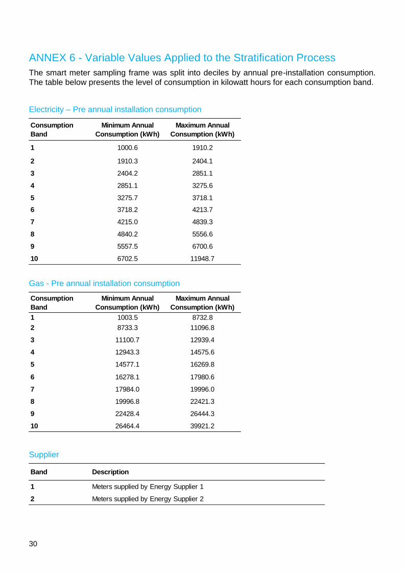
ANNEX 6 - Variable Values Applied to the Stratification Process
The smart meter sampling frame was split into deciles by annual pre-installation consumption. The table below presents the level of consumption in kilowatt hours for each consumption band.
Electricity – Pre annual installation consumption
Gas - Pre annual installation consumption
Supplier
Consumption
Band
Minimum Annual
Consumption (kWh)
Maximum Annual
Consumption (kWh)
1 1000.6 1910.2
2 1910.3 2404.1
3 2404.2 2851.1
4 2851.1 3275.6
5 3275.7 3718.1
6 3718.2 4213.7
7 4215.0 4839.3
8 4840.2 5556.6
9 5557.5 6700.6
10 6702.5 11948.7
Consumption
Band
Minimum Annual
Consumption (kWh)
Maximum Annual
Consumption (kWh)
1 1003.5 8732.8
2 8733.3 11096.8
3 11100.7 12939.4
4 12943.3 14575.6
5 14577.1 16269.8
6 16278.1 17980.6
7 17984.0 19996.0
8 19996.8 22421.3
9 22428.4 26444.3
10 26464.4 39921.2
Band Description
1 Meters supplied by Energy Supplier 1
2 Meters supplied by Energy Supplier 2

31
Geography
Residence Type – Experian Data
Size of Property (Number of Bedrooms) - Experian Data
Property Age - Experian Data
Household Income Group - Experian Data
Band Description
1 North (GOR North East, North West and Merseyside, Yorkshire and Humber)
2 Midlands (GOR East Midlands, West Midlands, East of England, Wales)
3 South (GOR South East, South West, London)
4 Scotland (GOR Scotland)
Band Description
1 Detached and Bungalow
2 Semi-Detached
3 Terraced and Flat
Band Description
1 1-2 bedrooms
2 3 bedrooms
3 4+ bedrooms
Band Description
1 Property built before and including 1954
2 Property built after 1954
Band Description
1 Less than £20,000 per annum
2 Between £20,000 and £40,000 per annum
3 Greater than £40,000 per annum

32
ANNEX 7 – Confidence Intervals
As the analysis employs a sampling approach, 95 per cent confidence intervals have been derived to demonstrate the robustness of consumption change estimates. Confidence intervals are influenced by the size of the sample analysed and the variation of the distribution of results. As Figure 3 illustrates, there is a significant reduction in consumption for smart meter customers for both electricity and gas but also showcases the uncertainty around these estimates. While the consumption reduction estimates have been obtained using the formulae in Section 5.6, which yields the percentage energy saving across every unit in the sample, the confidence intervals are deduced by fitting an Ordinary Least Squares log-linear model, that produces an estimate of the energy saving per household:
ln(𝑦𝑖𝑎 𝑦𝑖
𝑏) = 𝛼 + 𝛽𝐷𝑖 + 𝜀𝑖⁄ ,
where:
(𝑦𝑖𝑎 𝑦𝑖
𝑏⁄ ) is the ratio of energy consumption for each household (‘a’ represents the after
treatment, smart meter sample, and ‘b’ represents the before treatment (control group), traditional meter sample.)
𝛼 is the intercept term that returns an estimate of change in energy consumption
𝐷𝑖 is a dummy variable taking the value of 0 for a control group and 1 for the treatment group
𝛽 is an estimate for the impact of smart meters, and
𝜀𝑖 is the error term.
An array of calculations needs to be performed in order to fit the model described above. Each smart meter household in the sample has a variable that shows its pre-installation consumption and the post-installation consumption after a smart meter has been installed. Each traditional meter household has the same two variables but the pre- and post-installation consumption figures are set around an arbitrary installation date. The first step in fitting the model is to find the ratio of post-installation consumption over pre-installation consumption for each household in the smart and traditional meter household sample (this variable is known as ‘post_pre’). The next step is to take the natural log of this variable for each household, producing a new variable called ‘LnTrad’ for all traditional meters, and ‘LnSmart’ for all smart meter households. Taking the difference between these two items creates a new variable, ‘LnDiff’ which is the difference of ‘LnSmart’ minus ‘LnTrad’. The averages of the ‘lnTrad’ and ‘lnSmart’ variables are determined along with the variance of ‘Lndiff’. After these calculations, the model can be implemented.
To determine the estimate in the model, firstly, subtract the average of ‘LnSmart’ from the average of ‘LnTrad’ and then find the percentage change by applying the formula below:
%𝐶ℎ𝑎𝑛𝑔𝑒 = (𝑒(𝐴𝑣𝑒𝑟𝑎𝑔𝑒𝑜𝑓𝐿𝑛𝑇𝑟𝑎𝑑̅̅ ̅̅ ̅̅ ̅̅ ̅̅ ̅̅ ̅̅ ̅̅ ̅̅ ̅̅ ̅̅ ̅̅ ̅̅ ̅̅ −𝐴𝑣𝑒𝑟𝑎𝑔𝑒𝑜𝑓𝐿𝑛𝑆𝑚𝑎𝑟𝑡̅̅ ̅̅ ̅̅ ̅̅ ̅̅ ̅̅ ̅̅ ̅̅ ̅̅ ̅̅ ̅̅ ̅̅ ̅̅ ̅̅ ̅̅ ̅) − 1)× 100%
Secondly, calculate the standard errors by implementing the following:

33
log(𝑠. 𝑒. ) = √𝑉𝑎𝑟(𝐿𝑛𝐷𝑖𝑓𝑓)
𝑛
Finally, apply the standard formulae to determine the final confidence intervals:
𝐶𝑜𝑛𝑓.𝐼𝑛𝑡 = (𝑒(LnDiff±1.96×log(𝑠.𝑒.)) − 1)× 100%
ANNEX 8 – Address Match-rates
Smart Meter data was matched to NEED (National Energy Efficiency Database) in order to append a UPRN, which could then be matched to Experian data. The table below provides a match-rate summary.
Smart Electricity 97.32 Smart Electricity 97.58
Traditional Electricity 93.60 Traditional Electricity 95.64
Smart Gas 97.79 Smart Gas 98.14
Traditional Gas 93.96 Traditional Gas 94.31
Smart Electricity 97.32 Smart Electricity 97.58
Traditional Electricity 93.60 Traditional Electricity 95.64
Smart Gas 97.79 Smart Gas 98.14
Traditional Gas 93.96 Traditional Gas 94.31
Address Spine Match
Supplier 1 UPRN Match-rate percentage Supplier 2 UPRN Match-rate percentage
Experian Data Match
Supplier 1 UPRN Match-Rate percentage Supplier 2 UPRN Match-Rate percentage

34
Glossary of Terms
ACRONYM MEANING
AECOMArchitecture, Engineering, Consulting, Operations and
Maintenance Technology Corporation
CI Confidence Interval
DECC Department for Energy & Climate Change
EDRP Energy Demand Research Project
ELP Early Learning Project
GOR Government Office Region
HCF Hundred Cubic Feet
IA Impact Assessment
IHD In-home Display
kWh Kilowatt Hours
m3 Cubic meter
M&ES Monitoring and Evaluation Strategy
MPAN Meter Point Administration Number
MPRN Meter Point Reference Number
NEED National Energy Efficiency Data-Framework
ONS Office for National Statistics
PPM Pre-payment Customers
RCT Random Control Trial
SAS Statistical Analysis Software
SMED Smart Meter Evaluation Data Framework
SMETS Smart Meter Equipment Technical Specification
SMIP Smart Metering Implementation Programme
t , t -1, t+1The date of installation, one year prior to installation, one
year after installation
UCL University College London
UK United Kingdom
UPRN Unique Property Reference Number

35

© Crown copyright [2015]
Department of Energy & Climate Change
3 Whitehall Place
London SW1A 2AW
www.gov.uk/decc
URN 15D/081


