Smart Systems for Urban Water Demand Management Pantelis Sopasakis joint work with A.K. Sampathirao, P. Patrinos & A. Bemporad. IMT Institute for Advanced Studies Lucca Monte Verit´ a, Switzerland, 22-25 Aug 2016
Transcript
Smart Systems for Urban Water DemandManagement
Pantelis Sopasakisjoint work with A.K. Sampathirao, P. Patrinos & A. Bemporad.
IMT Institute for Advanced Studies LuccaMonte Verita, Switzerland, 22-25 Aug 2016
Today’s talk
We will learn how to:
I model water networks
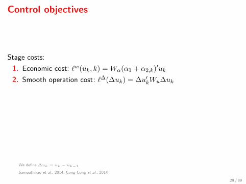
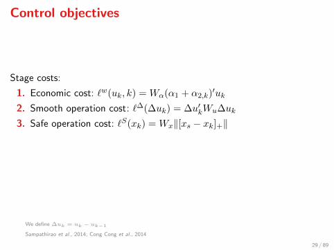
I identify control objectives
I make decisions under uncertainty
I formulate MPC problems
I devise algorithms to solve them
I parallelise them on GPUs
1 / 89
Introd
uctio
n
Con
trol
Alg
orith
ms
Simul
atio
ns
Wha
t to
mod
el
Lite
ratu
re o
verv
iew
Con
trol-o
rient
ed m
odel
s
Fore
cast
ing
The
MPC
con
cept
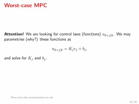
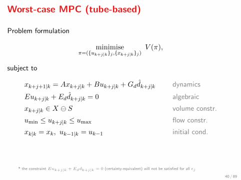
Wor
st-c
ase
MPC
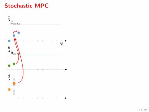
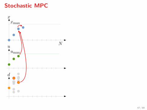
Stoc
hast
ic M
PCSc
enar
io-b
ased
MPC
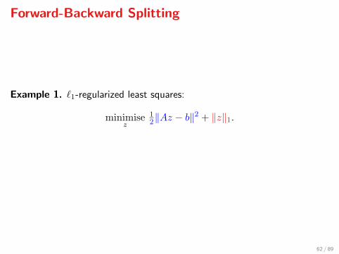
Prox
imal
ope
rato
r
Con
vex
conj
ugat
e
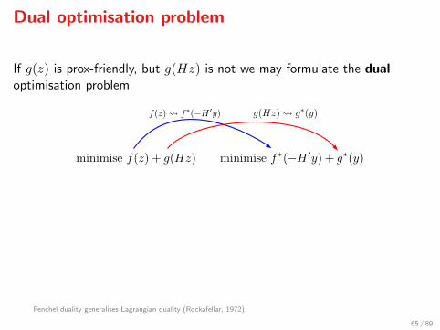
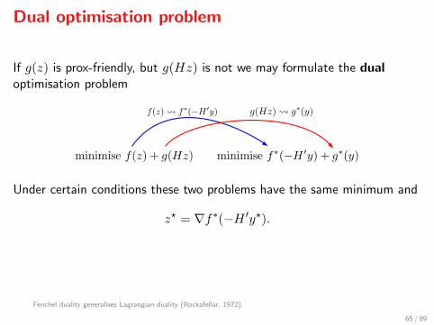
Dua
lity
APG
alg
orith
mD
WN
SM
PC p
robl
ems
Para
llelis
atio
n
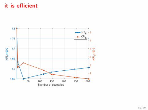
KPIs
Sim
ulat
ion
resu
ltsCon
clus
ions
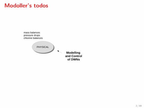
Modoller’s todos
Modelling and Control
of DWNs
PHYSICALPHYSICAL
mass balancespressure dropschlorine balances
2 / 89
Modoller’s todos
Modelling and Control
of DWNs
PHYSICALPHYSICAL
TIME SERIESTIME SERIES
mass balancespressure dropschlorine balances
seasonal ARIMABATS modelsneural networksSVM and other ML
3 / 89
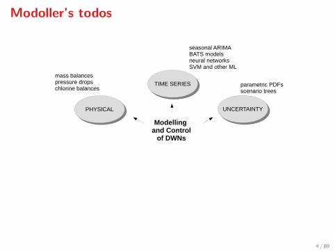
Modoller’s todos
Modelling and Control
of DWNs
PHYSICALPHYSICAL
TIME SERIESTIME SERIES
UNCERTAINTYUNCERTAINTY
mass balancespressure dropschlorine balances
seasonal ARIMABATS modelsneural networksSVM and other ML
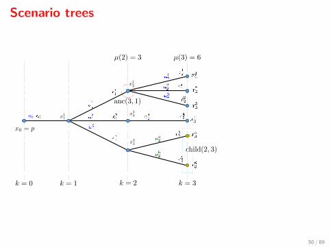
parametric PDFsscenario trees
4 / 89
Modoller’s todos
Modelling and Control
of DWNs
PHYSICALPHYSICAL
TIME SERIESTIME SERIES
UNCERTAINTYUNCERTAINTY
CONSTRAINTSCONSTRAINTS
mass balancespressure dropschlorine balances
seasonal ARIMABATS modelsneural networksSVM and other ML
parametric PDFsscenario trees
tanks pumps pressure drops
5 / 89
Modoller’s todos
Modelling and Control
of DWNs
PHYSICALPHYSICAL
TIME SERIESTIME SERIES
UNCERTAINTYUNCERTAINTY
CONSTRAINTSCONSTRAINTSOBJECTIVESOBJECTIVES
mass balancespressure dropschlorine balances
seasonal ARIMABATS modelsneural networksSVM and other ML
parametric PDFsscenario trees
tanks pumps pressure drops
energy consumptionoperating costsmoothness of actuationsafety storage
`
6 / 89
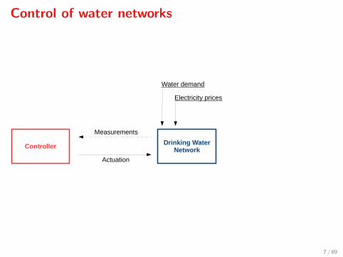
Control of water networks
ControllerDrinking Water
Network
Water demand
Electricity prices
Measurements
Actuation
7 / 89
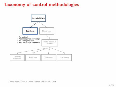
Taxonomy of control methodologies
Open Loop Closed Loop
CertaintyEquivalent Worst case Stochastic Risk-averse
Control of DWNs
● No feedback● Assumes perfect knowledge● No contingency plan● Requires human intervention Model Predictive
Control
Creasy 1998; Yu et al., 1994; Zessler and Shamir, 1989
8 / 89
Taxonomy of control methodologies
Open Loop Closed Loop
CertaintyEquivalent Worst case Stochastic Risk-averse
Control of DWNs
● Feedback compensates for modelling errors
Model Predictive Control
Creasy 1998; Yu et al., 1994; Zessler and Shamir, 1989
9 / 89
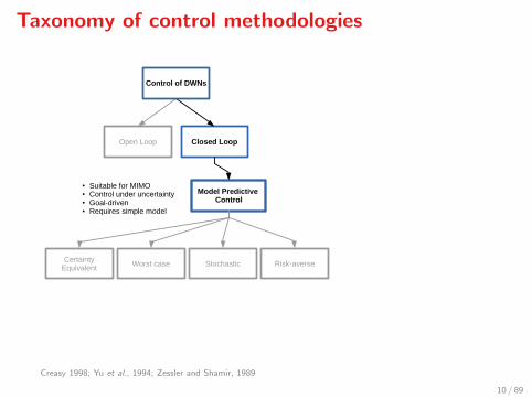
Taxonomy of control methodologies
Open Loop Closed Loop
Model Predictive Control
CertaintyEquivalent Worst case Stochastic Risk-averse
Control of DWNs
● Suitable for MIMO● Control under uncertainty● Goal-driven● Requires simple model
Creasy 1998; Yu et al., 1994; Zessler and Shamir, 1989
10 / 89
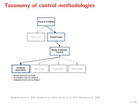
Taxonomy of control methodologies
Open Loop Closed Loop
CertaintyEquivalent Worst case Stochastic Risk-averse
Control of DWNs
● Model assumed accurate● Constraints may be violated● Suboptimal (we can do better)
Model Predictive Control
Sampathirao et al., 2014; Bakker et al., 2013; Leirens et al., 2010; Ocampo et al., 2009.
11 / 89
Taxonomy of control methodologies
Open Loop Closed Loop
CertaintyEquivalent Worst case Stochastic Risk-averse
Control of DWNs
● Pessimistic and conservative● Leads to small domain of attraction
Model Predictive Control
Ocampo et al., 2009 and 2010.
12 / 89
Taxonomy of control methodologies
Open Loop Closed Loop
CertaintyEquivalent Worst case Stochastic Risk-averse
Control of DWNs
● Makes use of probabilistic info● Less conservative, more realistic
Model Predictive Control
Sampathirao et al., 2014; Goryashko and Nemirovski, 2014; Tran and Brdys, 2009, Watkins and McKinney, 1997
13 / 89
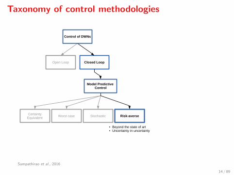
Taxonomy of control methodologies
Open Loop Closed Loop
CertaintyEquivalent Worst case Stochastic Risk-averse
Control of DWNs
● Beyond the state of art● Uncertainty in uncertainty
Model Predictive Control
Sampathirao et al., 2016
14 / 89
Objectives
To MODEL (water demands, hydraulics, uncertainty, etc), pose astochastic predictive CONTROL problem (define objectives, constraints)
and devise algorithms to SOLVE it numerically.
15 / 89
Intro
duct
ion
Con
trol
Alg
orith
ms
Simul
atio
ns
Wha
t to
mod
el
Lite
ratu
re o
verv
iew
Con
trol-o
rient
ed m
odel
s
Fore
cast
ing
The
MPC
con
cept
Wor
st-c
ase
MPC
Stoc
hast
ic M
PCSc
enar
io-b
ased
MPC
Prox
imal
ope
rato
r
Con
vex
conj
ugat
e
Dua
lity
APG
alg
orith
mD
WN
SM
PC p
robl
ems
Para
llelis
atio
n
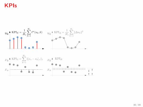
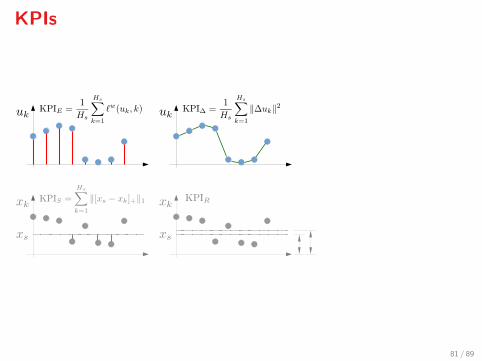
KPIs
Sim
ulat
ion
resu
ltsCon
clus
ions
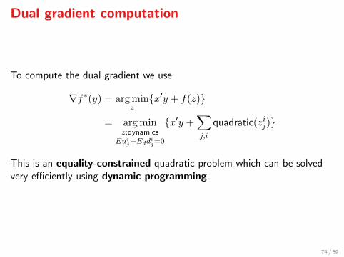
MPC
Control-oriented models
T1
T2
D1
T3
D2
16 / 89
Control-oriented models
T1
T2
D1
T3
D2
Actuation
17 / 89
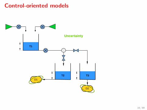
Control-oriented models
T1
T2
D1
T3
D2
Uncertainty
18 / 89
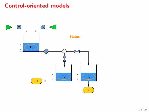
Control-oriented models
T1
T2
D1
T3
D2
States
19 / 89
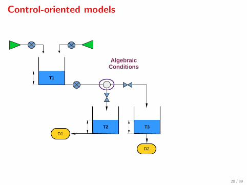
Control-oriented models
T1
T2
D1
T3
D2
Algebraic Conditions
20 / 89
Our case study
DWN of Barcelona: 63 tanks, 114 pumping stations and valves, 88 demand nodes & 17 pipe intersection nodes.
21 / 89
Control-oriented models
Simple mass balance equation (in discrete time)
xk+1 = Axk +Buk +Gddk,
0 = Euk + Eddk,
xk: tank volumes, uk: flows (controlled by pumping), dk: demands —along with the constraints
xmin ≤ xk ≤ xmax,
umin ≤ uk ≤ umax.
Sampathirao, Sopasakis et al., 2016, 2014; Wang et al., 2014; Ocampo et al., 2010; Ocampo et al., 2009.
22 / 89
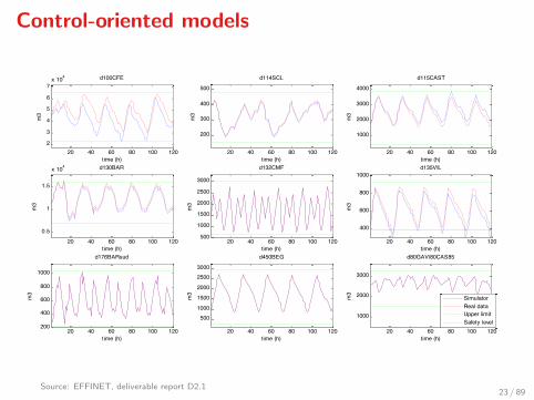
Control-oriented models
20 40 60 80 100 1202
3
4
5
6
7x 10⁴ d100CFE
time (h)
m3
20 40 60 80 100 120
200
300
400
500
d114SCL
time (h)
m3
20 40 60 80 100 120
1000
2000
3000
4000
d115CAST
time (h)
m3
20 40 60 80 100 120
0.5
1
1.5
x 104 d130BAR
time (h)
m3
20 40 60 80 100 120500
1000
1500
2000
2500
3000
d132CMF
time (h)
m3
20 40 60 80 100 120
400
600
800
1000d135VIL
time (h)
m3
20 40 60 80 100 120200
400
600
800
1000
d176BARsud
time (h)
m3
20 40 60 80 100 120
5001000
1500
2000
25003000
d450BEG
time (h)
m3
20 40 60 80 100 120
1000
2000
3000
d80GAVi80CAS85
time (h)m
3
SimulatorReal dataUpper limitSafety level
Source: EFFINET, deliverable report D2.123 / 89
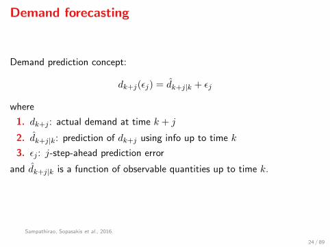
Demand forecasting
Demand prediction concept:
dk+j(εj) = dk+j|k + εj
where
1. dk+j : actual demand at time k + j
2. dk+j|k: prediction of dk+j using info up to time k
3. εj : j-step-ahead prediction error
and dk+j|k is a function of observable quantities up to time k.
Sampathirao, Sopasakis et al., 2016.
24 / 89
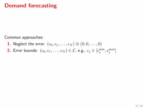
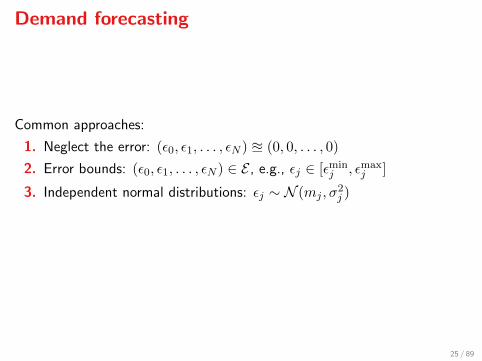
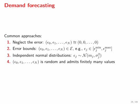
Demand forecasting
Common approaches:
1. Neglect the error: (ε0, ε1, . . . , εN ) u (0, 0, . . . , 0)
1. A. Sampathirao, P. Sopasakis, A. Bemporad, and P. Patrinos, “Fast parallelizable scenario-based stochasticoptimization,” EUCCO 2016, Leuven, Belgium, 2016.
2. A. Sampathirao, P. Sopasakis, A. Bemporad, and P. Patrinos, “GPU-accelerated stochastic predictive control of drinkingwater networks,” IEEE CST (submitted, provisionally accepted), 2016 (on arXiv).
3. A. Sampathirao, J. Grosso, P. Sopasakis, C. Ocampo-Martinez, A. Bemporad, and V. Puig, “Water demand forecastingfor the optimal operation of large-scale drinking water networks: The Barcelona case study,” 19th IFAC World Congress,pp. 10457–10462, 2014.
4. A. Sampathirao, P. Sopasakis, A. Bemporad, and P. Patrinos, “Distributed solution of stochastic optimal controlproblems on GPUs, 54th IEEE Conf. Decision and Control, (Osaka, Japan), Dec 2015.
5. A. Sampathirao, P. Sopasakis, A. Bemporad, and P. Patrinos, “Proximal Quasi-Newton Methods for Scenario-basedStochastic Optimal Control,” IFAC 2017 (submitted).
6. M. Bakker, J. H. G. Vreeburg, L. J. Palmen, V. Sperber, G. Bakker, and L. C. Rietveld, “Better water quality and higherenergy efficiency by using model predictive flow control at water supply systems,” J Wat Supply: Research &Technology – Aqua, 62(1), pp. 1–13, 2013.
7. S. Leirens, C. Zamora, R. Negenborn, and B. De Schutter, “Coordination in urban water supply networks usingdistributed model predictive control,” ACC 2010, (Baltimore, USA), pp. 3957–3962, 2010.
8. C. Ocampo-Martinez, V. Puig, G. Cembrano, R. Creus, and M. Minoves, “Improving water management efficiency byusing optimization-based control strategies: the barcelona case study,” Water Science and Technology: Water Supply,9(5), pp. 565–575, 2009.
9. C. Ocampo-Martinez, V. Fambrini, D. Barcelli, and V. Puig, “Model predictive control of drinking water networks: Ahierarchical and decentralized approach,” ACC 2010, (Baltimore, USA), pp. 3951–3956, 2010.
10. A. Goryashko and A. Nemirovski, “Robust energy cost optimization of water distribution system with uncertaindemand,” Automation and Remote Control 75(10), pp. 1754–1769, 2014.
11. U. Zessler and U. Shamir, “Optimal operation of water distribution systems,” J Wat Resour Plan & Mngmt, 115(6), pp.735–752, 1989.
88 / 89
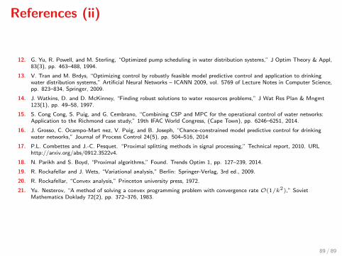
References (ii)
12. G. Yu, R. Powell, and M. Sterling, “Optimized pump scheduling in water distribution systems,” J Optim Theory & Appl,83(3), pp. 463–488, 1994.
13. V. Tran and M. Brdys, “Optimizing control by robustly feasible model predictive control and application to drinkingwater distribution systems,” Artificial Neural Networks – ICANN 2009, vol. 5769 of Lecture Notes in Computer Science,pp. 823–834, Springer, 2009.
14. J. Watkins, D. and D. McKinney, “Finding robust solutions to water resources problems,” J Wat Res Plan & Mngmt123(1), pp. 49–58, 1997.
15. S. Cong Cong, S. Puig, and G. Cembrano, “Combining CSP and MPC for the operational control of water networks:Application to the Richmond case study,” 19th IFAC World Congress, (Cape Town), pp. 6246–6251, 2014.
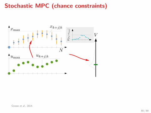
16. J. Grosso, C. Ocampo-Mart nez, V. Puig, and B. Joseph, “Chance-constrained model predictive control for drinkingwater networks,” Journal of Process Control 24(5), pp. 504–516, 2014
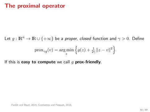
17. P.L. Combettes and J.-C. Pesquet. “Proximal splitting methods in signal processing,” Technical report, 2010. URLhttp://arxiv.org/abs/0912.3522v4.
18. N. Parikh and S. Boyd, “Proximal algorithms,” Found. Trends Optim 1, pp. 127–239, 2014.
19. R. Rockafellar and J. Wets, “Variational analysis,” Berlin: Springer-Verlag, 3rd ed., 2009.
20. R. Rockafellar, “Convex analysis,” Princeton university press, 1972.
21. Yu. Nesterov, “A method of solving a convex programming problem with convergence rate O(1/k2),” SovietMathematics Doklady 72(2), pp. 372–376, 1983.