Smart water management (SWM): flood control and water uses Filipa Henriques de Oliveira Caleiro Thesis for obtaining the Master of Science Degree in Civil Engineering Supervisor: Professor Helena Margarida Machado da Silva Ramos Examination Committee Chairperson: Professor António Alexandre Trigo Teixeira Supervisor: Professor Helena Margarida Machado da Silva Ramos Members of the Committee: António Jorge Silva Guerreiro Monteiro July 2016
Transcript
Smart water management (SWM): flood control and water
uses
Filipa Henriques de Oliveira Caleiro
Thesis for obtaining the Master of Science Degree in
Civil Engineering
Supervisor: Professor Helena Margarida Machado da Silva Ramos
Examination Committee
Chairperson: Professor António Alexandre Trigo Teixeira
Supervisor: Professor Helena Margarida Machado da Silva Ramos
Members of the Committee: António Jorge Silva Guerreiro Monteiro
July 2016
Smart water management (SWM): flood control and water uses
ii
Smart water management (SWM): flood control and water uses
iii
Acknowledgment
This dissertation is the final conclusion of this part of my academic life and is a result of great effort
and sacrifice not only on my part but also by those who supported me during this journey.
First of all I would like to thank to my MSc supervisor, Prof. Helena Ramos, for giving me the
opportunity to work in an area that interests me. She gave me all the flexibility to be independent and
creative and was very supportive, guiding and advising me throughout the entire process. I could
always rely on her to ask the questions that needed to be answered and point me in the right direction
so I could find the solution and eventually learn what questions I should be asking myself.
I also want to thank to Eng. Cecília Correia for providing the license of DHI’s MIKE SHE software
without which this investigation would be much more difficult and for all the interest and availability to
answer my questions.
I would also like to thank all other professors that I had the pleasure of taking classes from while at
Instituto Superior Técnico.
Lastly, and most importantly I would like to thank my family for providing continual support throughout
this journey and for all the sacrifices they made so I could finish my studies. I would especially like to
thank my fiancé, José Reis, for his understanding and patience dealing with long nights, weekends
and all the long hours studying. He has always been there for me and I look forward to be there for
him as well.
Smart water management (SWM): flood control and water uses
iv
Smart water management (SWM): flood control and water uses
v
Abstract
The main objective of this work is to analyse a study area, in Seixal, regarding flood risk and flood
mitigation techniques. This analysis was performed by computational modelling using DHI software,
MIKE SHE. Several scenarios were compared regarding flood risk and SUDS efficiency. To obtain a
more accurate analysis was also determined the economic viability of each technique. The flood
mitigation capacity of each type of SUDS technique was considered, as well as the community
acceptance to their construction and maintenance. Considering factors such as vulnerability to flood
and quantity of flooded area, the objective was to define the most efficient system to solve flood
situations in Seixal bay. The economic viability of the different scenarios was stablished in two ways:
the first one through life cost analysis and the second one taking into account the damages caused
by a certain type of flood.
Finally, it was concluded that the best scenario is the one who will minimize the effects of great
urbanization and consequently the increase of flood risk, which combines two different measures:
permeable pavement and detention basin. This alternative allows to fully explore the mitigation
capacity of each technique. The installation of this system proved to be viable, demonstrating a very
important improvement in the flood mitigation system in Seixal.
Smart water management (SWM): flood control and water uses
vi
Smart water management (SWM): flood control and water uses
vii
Resumo
O principal objetivo deste trabalho é analisar uma área de estudo, localizada no Seixal, relativamente
ao risco de cheia e formas de mitigação de cheia. Esta análise foi realizada por modelação
computacional com recurso ao software da DHI, MIKE SHE. Vários cenários foram comparados
quanto ao risco de inundação e eficiência na aplicação de sistemas de drenagem urbana sustentável,
bem como uma avaliação da viabilidade económica de cada sistema de drenagem aplicado em cada
cenário. A influência de cada tipo de sistema de drenagem na mitigação da cheia foi determinada,
assim como a análise de sensibilidade da comunidade relativamente à sua aplicação e manutenção
nos locais determinados. Tendo em conta fatores como a vulnerabilidade da zona de estudo e a
quantidade de zona inundada, o objetivo foi determinar qual o sistema mais eficiente para solucionar
situações de cheia. O estudo de viabilidade económica dos diferentes cenários foi abordado de duas
formas distintas, a primeira através da análise de custo de ciclo de vida, e a segunda tendo em conta
os danos causados por uma cheia tipo.
Por fim, verificou-se que para a área de estudo o cenário que melhor minimizará os efeitos
decorrentes da grande urbanização e consequente aumento do risco de cheia, passa pela conjugação
de diferentes medidas, nomeadamente aplicação de pavimento permeável e construção de uma bacia
de detenção, permitindo assim tirar o máximo partido das medidas mitigadoras. A instalação deste
sistema provou ser viável, o que significa um melhoramento futuro muito importante no sistema de
mitigação de cheia no Seixal.
Palavras-chave: Inundações urbanas, cheias, modelação, sistemas de drenagem urbana
sustentável, viabilidade económica.
Smart water management (SWM): flood control and water uses
viii
Smart water management (SWM): flood control and water uses
ix
Contents
Acknowledgment ............................................................................................................................... iii
Abstract ................................................................................................................................................ v
Resumo .............................................................................................................................................. vii
Contents .............................................................................................................................................. ix
List of Figures .................................................................................................................................... xi
List of tables ..................................................................................................................................... xiii
Abbreviations ................................................................................................................................... xiv
Table 6.8 - Total Cost ......................................................................................................................... 51
Table 6.9 - Weighting system ............................................................................................................. 52
Table 6.10 - Comparison between estimated damage costs for different simulated scenarios ......... 52
Smart water management (SWM): flood control and water uses
xiv
Abbreviations
APA
Agência Portuguesa do Ambiente
DHI
Danish hydrological institute
EEA
Europe Environmental Agency
EU
European Union
PoMs
Programmes of Measures
RBDs
River Basin Directives
RBMPs
River Basin Management Plans
SUDS Sustainable Urban Drainage System
UWM
Urban Water Management
WFD
Water Framework Directive
Smart water management (SWM): flood control and water uses
1
1. Introduction
1.1. Framework and motivation
Urban drainage systems are in transition from functioning simply as a transport system to becoming
an important element of urban flood protection measures (DHI, 2015).
Rapid urbanization combined with the implications of climate change is one of the major challenges
facing society nowadays and in the years to come. The increased concerns with water security and
ageing of existing drainage infrastructure, have created a valuable opportunity to address these water
challenges within cities and to improve urban water management.
Urban water management must ensure access to water and sanitation infrastructure and services,
manage rain, waste and storm water as well as runoff pollution, mitigate against floods, droughts and
water borne diseases, whilst prevent the resource from degradation. Urban water management takes
into consideration the water cycle, facilitates the integration of water factors early in the land planning
process and encourages all levels of government and industry to adopt water management and urban
planning practices that benefit the community, the economy and the environment.
Floods are the most common type of natural disaster in Europe (EEA, 2015). Flooding often occurs
as a result of high rainfall intensity in the catchment area, insufficient storm drainage capacity, river
overflows, storm surge or as a combination of these phenomena. The risks of flooding are amplified
by the expected effects of climate change and by the increase of impervious areas. The use of
sustainable urban drainage systems (SUDS) can reduce urban surface water flooding as well as the
pollution impact of urban discharges on receiving waters.
SUDS are more sustainable than conventional drainage techniques, offering benefits such as
attenuation of runoff prior to concentration, improvement of water quality, maintenance of groundwater
recharge rates through infiltration, minimization of flood impacts on the environment.
In the next few years, it is expected that cities will face resource distribution challenges associated
with an increase in population flow, energy issues due to the reduction of fossil fuel resources,
escalation maintenance and management costs due to aging infrastructure and improper land
resource utilization. Innovative and new sustainable systems are essential to minimize the impact of
these challenges.
Smart water management (SWM): flood control and water uses
2
1.2. Objectives
The main objectives of this work are to give an overview of urban water issues and smart water
management as well as the information about possible implementation of sustainable urban drainage
systems towards a more sustainable water management.
To achieve the proposed goals is performed an analysis of a case study assisted by a model simulation
software (MIKE SHE, by DHI) that allows to represent the benefits of these innovative and sustainable
systems. The current research work aims to demonstrate the susceptibility to flood of an area in the
old city center of Seixal, ways to prevent these extreme events in the area using sustainable urban
drainage systems and a cost/benefit analysis of its implementation.
1.3. Structure of the dissertation
The present dissertation is divided into seven chapters. The first chapter corresponds to the
introduction, where a scope to address the subject is made and the main objectives are presented. In
chapter 2 an overview of the Water Framework Directive and its implementation in Portugal is
presented. Also in this chapter is presented some information about floods and its influence in Europe
as well as particularities about sustainable urban drainage systems and criteria for selecting the
technique for each type of situation. The simulation model and theoretical fundaments of MIKE SHE
are presented in Chapter 3. The case study description and methodology are presented in Chapter 4,
describing the study area and the Tagus estuary characteristics. Chapter 5 presents the model testing
and validation, specifying all the used input data as well as the scenario simulations obtained for each
technique and also the assessment of the best scenario. Chapter 6 presents an economic analysis
concerning the viability of SUDS implementation in the case study in two different views: life cost
analysis and damage analysis. The last chapter (chapter 7) presents the general conclusions of this
thesis and some recommendations for future works.
Smart water management (SWM): flood control and water uses
3
2. State-of-the-art
2.1. Water Framework Directive and its implementation in Portugal
The Water Framework Directive (WFD) adopted in 2000 established an integrated approach for
European Union (EU) members action in the field of water policy. It is centered on the concept of river
basin management with the objective of achieving good status of all EU waters by 2015.
The main tools to implement the Directive are the River Basin Management Plans (RBMPs) and the
Programmes of Measures (PoMs), which are updated every six years. The River Basin Management
Plans and Programmes of Measures, adopted in 2009, are being updated and their final adoption will
be by the end of 2015. Examples of measures are: to reduce point source or diffuse pollution,
rehabilitation of hydromorphological conditions, protect water bodies, improve aquifer recharge,
measures addressing efficient water use, control on water abstraction and discharges. Measures are
presented by type (basic, supplementary, complementary and additional); by operational programme
(national programmes and plans); by theme (water quantity, monitoring and research); and by
responsible entity (Directive 2000/60/EC).
The EU Commission’s assessment shows that many Member States have planned their measures
based on ‘what is in place and/or in the pipeline already’ and ‘what is feasible’. Instead of designing
the most appropriate and cost-effective measures to ensure that their water achieves ‘good status’,
many Member States have often only estimated how far current measures will contribute to the
achievement of the WFD’s environmental objectives. This leads to a non-clear evaluation of whether
measures are taken to progress required by the Directive 2000/60/EC.
Excessive abstraction significantly affects 10 % of surface water bodies and 20 % of groundwater
bodies. Where there is already over-abstraction in river basins subject to intense water use, the WFD
requires Member States to put in place measures that restore the long-term sustainability of
abstraction such as revision of permits or better enforcement. The first RBMPs also showed that most
Member States have not addressed the water needs of nature. They often considered only the
minimum flows to be maintained in summer periods, without taking into account the different factors
that are critical for ecosystems to thrive and to deliver their full benefits. This means that the measures
implemented do not guarantee the achievement of ‘good status’ in many water bodies affected by
significant abstractions or flow regulation (e.g. for irrigation, hydropower, drinking water supply,
navigation). Changes to the flow and physical shape of water bodies are among the main factors
preventing the achievement of good water status but, in general, the first PoMs propose insufficient
actions to counter this. The changes are most often due to the development of grey infrastructure,
such as land drainage channels, dams for irrigation or hydropower, impoundments to facilitate
navigation, embankments or dykes for flood protection (Directive 2000/60/EC).
Smart water management (SWM): flood control and water uses
4
The Floods Directive of 2007 aims to reduce and manage the risks that floods pose to human health,
the environment, cultural heritage and economic activity. By 2015 flood risk management plans must
be drawn up for areas identified to be at risk. Unlike the WFD, the Floods Directive does not have a
precise calendar of public consultation, but many Member States will consult on the WFD and Flood
Plans at the same time, during the first semester of 2015. Natural water retention measures are an
example of measures that can contribute simultaneously to the achievement of objectives under the
WFD and the FD by strengthening and preserving the natural retention and storage capacity of
aquifers, soils and ecosystems. Measures such as the reconnection of the floodplain to the river, re-
meandering, and the restoration of wetlands can reduce or delay the arrival of flood peaks downstream
while improving water quality and availability, preserving habitats and increasing resilience to climate
change. Fluvial is the most common reported source of flooding in the EU, followed by pluvial and sea
water. The most commonly reported consequences are economic, followed by those for human health.
Only one third of Member States explicitly considered long-term developments in their assessment of
flood risk, although the flood losses in Europe have increased substantially in recent decades,
primarily due to socio-economic factors such as increasing wealth located in flood-prone areas, and
due to a changing climate. It was estimated that by 2007, at least 11 % of Europe's population and 17
% of its territory had been affected by water scarcity, putting the cost of droughts in Europe over the
past thirty years at EUR 100 billion. The EU Commission expects further deterioration of the water
situation in Europe if temperatures keep rising as a result of climate change. The Programmes of
Measures also confirm that incentives to use water efficiently and transparent water pricing are not
applied across all Member States and all water-using sectors, partly due to the lack of metering. In
order to implement incentive pricing, consumptive uses should by default be subject to volumetric
charges based on real use. This requires widespread metering, in particular for agriculture in basins
where irrigation is the main water user. Measures to ensure the recovery of environmental and
resource costs are limited and needed. There is an absence of cost recovery, including for
environmental, resource and infrastructure costs, which will affect those areas facing water scarcity
and failing water infrastructure. In this context, the EU Commission is carrying out an assessment of
Member States’ water pricing and cost recovery policies and requires action plans where deficiencies
are detected (Directive 2007/60/EC).
There are three different administrative jurisdictions governing the Water Framework Directive
implementation in Portugal: mainland Portugal (PTRH1 to PTRH8) governed by the Portuguese
Environmental Agency (APA), the Azores (PTRH9) and Madeira (PTRH10) governed by the
respective autonomous region environment authority. According to the RBDMPs, in terms of surface
waters, some water bodies are subject to significant pressures from diffuse source pollution. All RBDs
except Madeira have some water bodies subjected to water flow regulations and morphological
alterations. Most of the jurisdictions have some water bodies subjected to significant pressures from
water abstraction. Saltwater intrusion pressure is reported to be significant in Azores. In terms of status
of surface water, 57% of natural water bodies and 28% of heavily modified/artificial water bodies were
reported to be in good or better ecological status/potential, and 24% of natural surface water bodies
and 30% of heavily modified/artificial water bodies were at good chemical status. It is expected that
Smart water management (SWM): flood control and water uses
5
by 2015, about 60% of all water bodies will be in good or better status/potential. In terms of
groundwater in 2009, 82% of the groundwater bodies were reported to be at good chemical status and
98 % at good quantitative status. Nitrate was considered to be the most challenging factor. The
significant pressure is therefore agriculture and livestock. In 2015 it is expected that 85% of
groundwater will achieve good chemical status while the quantitative status is maintained at their very
high 2009 level. Overall RBDs reported by Portugal, 80% of basic measures were on-going and 20%
not started. No measures had been completed. In particular the Northern Regional Department have
not started the implementation of several types of measures. For some types of measures - e.g.
Prohibition of direct discharge of pollutants into groundwater - the RBD have changed their views
regarding applicability of the measures. Figure 2.1 shows the reported progress of basic measures in
Portugal so far (Report on the progress in implementation of the WFD PoMs).
Figure 2.1 - Reported progress with implementation of basic measures (WISE PoMs Aggregation Report 2-2 - Implementation of Other Basic Measures in 2012)
Further consultation with the water authority indicates that about 58% of the measures being
implemented in Portugal use EU Structural Funds, while 5% uses Rural Development Fund and 1%
uses Cohesion funds. About 39% of the measures are not using EU funds. (Report on the progress in
implementation of the WFD PoMs)
Supplementary Measures are those measures designed and implemented in addition to the Basic
Measures where they are necessary to achieve the environmental objectives of the WFD.
Supplementary Measures can include additional legislative powers, fiscal measures, research or
educational campaigns that go beyond the Basic Measures and are deemed necessary for the
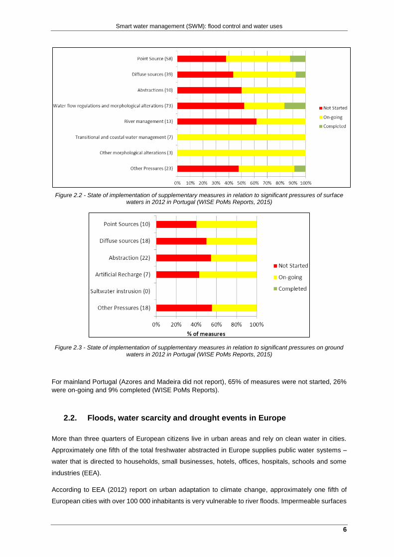
achievement of objectives. (Report on the progress in implementation of the WFD PoMs) Figure 2.2
and Figure 2.3, shows the progress of implementation of supplementary measures in Portugal, in
surface waters and ground water, respectively. Number in brackets is the number of supplementary
measures tackling the pressure. Note a measure may tackle more than one pressure.
Smart water management (SWM): flood control and water uses
6
Figure 2.2 - State of implementation of supplementary measures in relation to significant pressures of surface waters in 2012 in Portugal (WISE PoMs Reports, 2015)
Figure 2.3 - State of implementation of supplementary measures in relation to significant pressures on ground waters in 2012 in Portugal (WISE PoMs Reports, 2015)
For mainland Portugal (Azores and Madeira did not report), 65% of measures were not started, 26%
were on-going and 9% completed (WISE PoMs Reports).
2.2. Floods, water scarcity and drought events in Europe
More than three quarters of European citizens live in urban areas and rely on clean water in cities.
Approximately one fifth of the total freshwater abstracted in Europe supplies public water systems –
water that is directed to households, small businesses, hotels, offices, hospitals, schools and some
industries (EEA).
According to EEA (2012) report on urban adaptation to climate change, approximately one fifth of
European cities with over 100 000 inhabitants is very vulnerable to river floods. Impermeable surfaces
Smart water management (SWM): flood control and water uses
7
(‘soil sealing’) can prevent water from draining, leading to increased risk of flooding. However, it is
important to be aware that impermeable surfaces are only one factor contributing to increased risk of
urban flooding, the increase of temperature and extreme precipitation events could also explain this
changes.
The map in Figure 2.4, shows the average soil sealing degree inside of European core cities. Soil
sealing degrees are represented in colored dots. The city dots are overlaid onto a modelled map
displaying the change in annual number of days with heavy rainfall between the reference periods
1961-1990 and 2071-2100.
Figure 2.4 - Average soil sealing degree inside of European core cities (European Environment Agency, 2015)
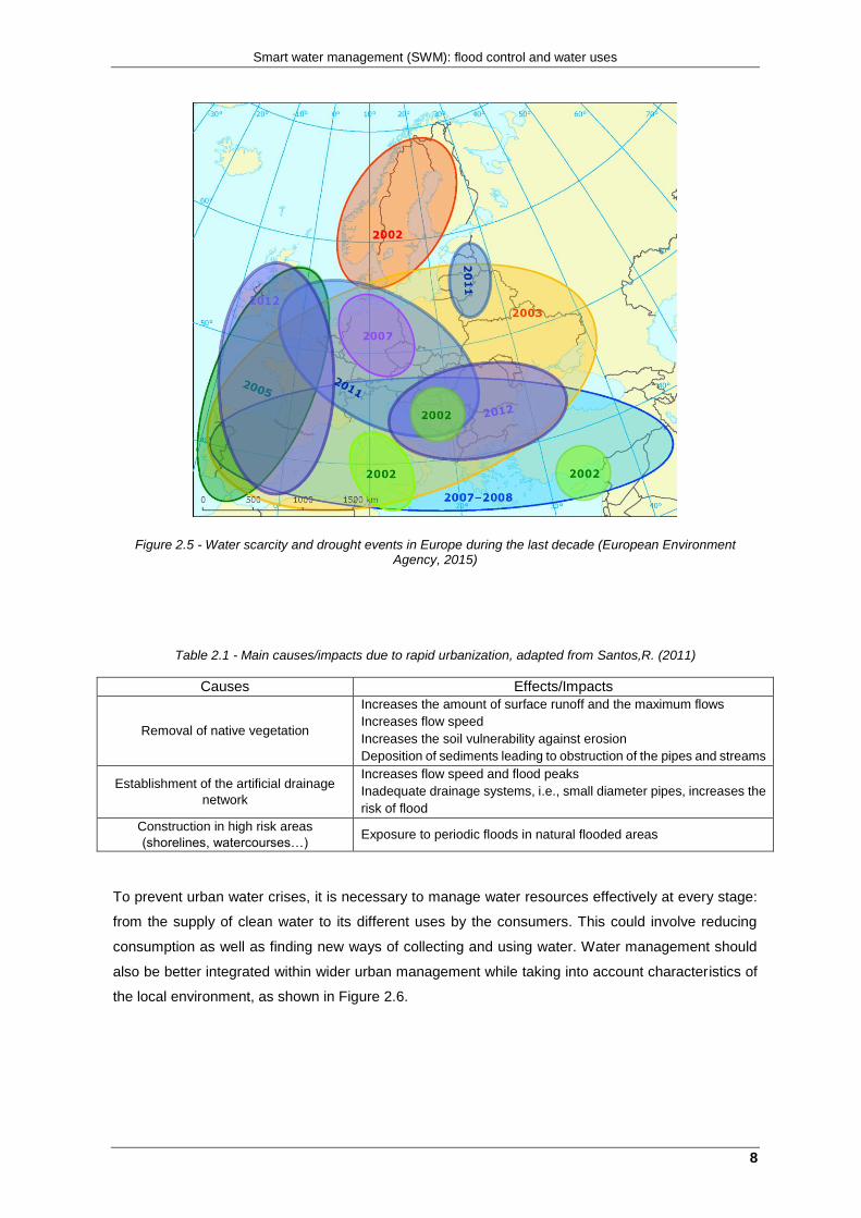
Regions most prone to an increase in drought hazard are southern and south-eastern Europe, but
minimum river flows will also decrease significantly in many other parts of the continent, especially in
summer, Figure 2.5.
Smart water management (SWM): flood control and water uses
8
Figure 2.5 - Water scarcity and drought events in Europe during the last decade (European Environment Agency, 2015)
Table 2.1 - Main causes/impacts due to rapid urbanization, adapted from Santos,R. (2011)
Causes Effects/Impacts
Removal of native vegetation
Increases the amount of surface runoff and the maximum flows
Increases flow speed
Increases the soil vulnerability against erosion
Deposition of sediments leading to obstruction of the pipes and streams
Establishment of the artificial drainage
network
Increases flow speed and flood peaks
Inadequate drainage systems, i.e., small diameter pipes, increases the
risk of flood
Construction in high risk areas
(shorelines, watercourses…) Exposure to periodic floods in natural flooded areas
To prevent urban water crises, it is necessary to manage water resources effectively at every stage:
from the supply of clean water to its different uses by the consumers. This could involve reducing
consumption as well as finding new ways of collecting and using water. Water management should
also be better integrated within wider urban management while taking into account characteristics of
the local environment, as shown in Figure 2.6.
Smart water management (SWM): flood control and water uses
9
Figure 2.6 - Effects of imperviousness on runoff and infiltration, adapted from US EPA (2015)
2.3. Flood types
A river flood typically occur in large basins and is the result of natural processes, in which the river
takes its larger bed. Usually caused by long periods of rain.
Storm surge is an abnormal rise in water level in coastal areas, over and above the regular
astronomical tide, caused by forces generated from a severe storm's wind, waves, and low
atmospheric pressure. Extreme flooding can occur in coastal areas particularly when storm surge
coincides with normal high tide.
Storm tide is a rise in local sea level caused by the combination of regular tides and a storm surge.
Inland flooding occurs when moderate precipitation accumulates over several days, intense
precipitation falls over a short period, or a river overflows because of an ice or debris jam or dam
failure.
A flash flood is caused by heavy or excessive rainfall in a short period of time, generally less than six
hours. They can occur within minutes or a few hours of excessive rainfall. This type of phenomenon
in urban areas is growing, which combined with surfaces unable to absorb large amounts of water in
such short period of time, increases the flow velocity and the destructive potential.
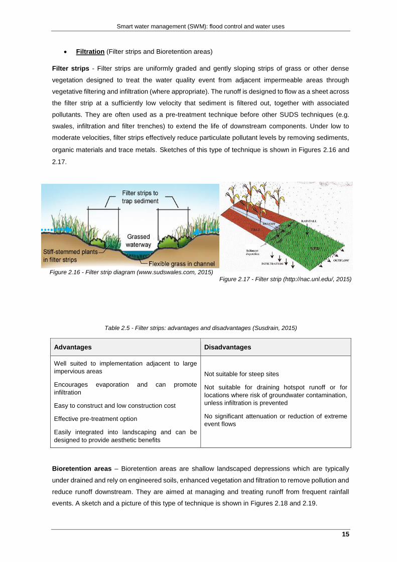
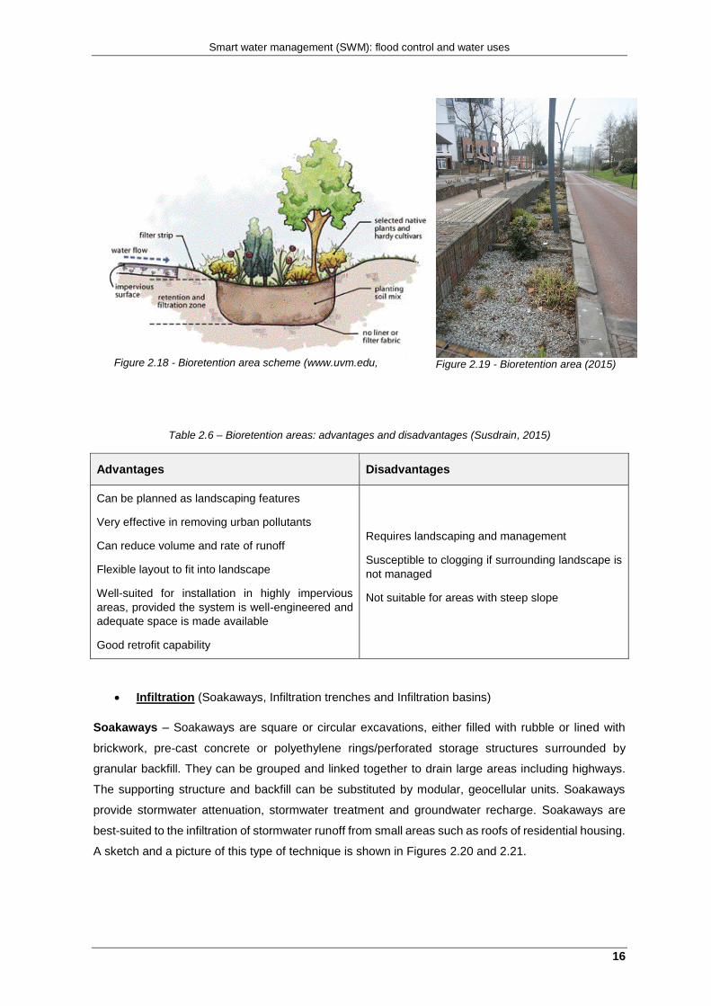
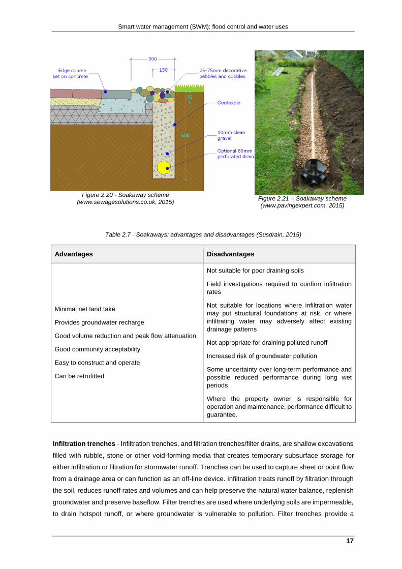
Table 2.12 - Wetlands: advantages and disadvantages (Susdrain, 2015)
Advantages Disadvantages
Good removal capability or urban pollutants
If lined, can be used where groundwater is
vulnerable
Good community acceptability
High potential ecological, aesthetic and amenity
benefits
May add value to local property.
Land take is high
Requires baseflow
Limited depth range for flow attenuation
May release nutrients during non-growing season
Little reduction in run volume
Not suitable for steep sites
Colonization by invasive species would increase
maintenance
Performance vulnerable to high sediment inflows.
Smart water management (SWM): flood control and water uses
23
3. Simulation model
3.1 MIKE SHE software
A hydrologic and hydrodynamic models are used to understand why a flow system is behaving in a
particular way and to predict how a flow system will behave in the future (Fetter, 2001). These two
uses, understanding observed flow and predicting future behavior, are integral in creating real world
infrastructure that will be able to sustainably exist within the hydrologic and hydraulic systems. Models
can be classified as physical, analog, or mathematical in nature. Mathematical models can be
represented in a number of ways depending on the input output relationships and what laws and
principles they abide by. A mathematical model can use theoretical equations that follow the laws of
nature and be classified as physically based, or the model can use experimental based relationships
to draw equations and be classified as empirically based. A model that spatially or temporally varies
the input parameters is a distributed model, in contrast to a lumped model, which has a spatially or
temporally uniform input parameter set. Models can also either be event based which simulate a
particular event of process for a short period; or a model can be continuous in nature and output
several years’ worth of data. The extent to which model parameters are determined can further classify
models. A deterministic model has every parameter fully determined by governing equations, a
stochastic or probabilistic model has incomplete determination and some variable are totally or
partially described by probability equations (DHI, 2004).
MIKE SHE is a fully integrated, physically based, distributed model, capable of both event based and
continuous simulations. The model is able to simulate hydrology in plot, field, and watershed scales,
particle tracking of solutes, and can be linked with MIKE 11 to simulate watershed-river relationships.
The MIKE SHE model was originally developed by three European organizations (Danish Hydraulic
Institute, British Institute of Hydrology, and a French consulting company SOGREAH) in 1977. DHI
has taken the lead in development and research of MIKE SHE for improvements and additions (DHI,
2004).
The physically based nature of the model lends inclusion of natural topography and watershed
characteristics such as vegetation, soil, and weather parameter sets. The distributed nature of the
model allows the user to spatially and temporally vary parameter sets such as soil profiles, land use
conditions, drainage practices, weather and evapotranspiration data sets, and overland flow values.
The spatial distribution is accomplished through an orthogonal grid network that allows for horizontal
or vertical discretization, as applicable within each parameter set (Abbot et al., 1986).
Temporal distribution allows users to either vary parameters by time step, or set constant values for
parameters for the entirety of the simulation period. The user can also change the complexity of the
model simulation by adjusting the modular setup of the model within the GUI (graphic user interface).
One can choose to include the modules such as Overland Flow (OF), Rivers and Lakes (OC),
Unsaturated Zone (UZ), Evapotranspiration (ET), and Saturated Flow (SF). If the saturated flow
Smart water management (SWM): flood control and water uses
24
module is included than the unsaturated zone and evapotranspiration modules must be included as
well.
3.2 MIKE SHE in drainage applications
A series of research studies (Al-Khudhairy, et al 1997, 1999, Thompson, et al 2004) investigated the
effects of changes in hydrology of marshland in Southeast England. The former two works address a
10 km2 area near the North Kent Marshes; the later paper by Thompson (2004) addresses the adjacent
8.7 km2 of the Elmey Marshes on the Isle of Sheppey. This marshland was drained for grazing in the
past century and the authors were investigating the effects that restoration of the ground to its former
state would have (Al-Khudhairy, 1997; Thompson, 2004). A pseudo-differential split sample was used
to assess the MIKE SHE predictions of the effects on hydrology of changes in land use. Coefficient of
correlation values for observed monthly flow reached 0.87 for the baseline model flow and 0.92 with
the baseline model with macropore flow. These results support Jayatilaka’s conclusion that shrink-
swell characteristics of soil profiles are important in describing preferential flow in the unsaturated
zone (Al-Khudhairy, 1999). Thompson (2004) found that the coupling MIKE SHE with MIKE 11 to
describe marshland piezometric head and surface water extent lead to a high degree of precision.
Observed head values at piezometer locations throughout the research area had coefficients of
correlation ranging from 0.41 to 0.78 for testing and 0.56 to 0.92 for validation. Thompson (2004)
concluded that the MIKE SHE model was sufficient to describe the water table elevation of marshland
in the Southeastern region of England and postulated that it may be sufficient to model marshland
area in other regions as well.
Several investigators have used MIKE SHE in dissimilar conditions to analyze and develop solutions
to hydrological problems within the parent region. In the mountainous regions of Hawaii, irrigation is
less of an issue than flash flooding resulting from short but intense rainfall events (Sahoo, 2004). The
study area investigated included two watersheds in the Manoa-Palolo stream system adding up to
27.28 km2 on the Hawaiian island of Oahu. Flow data was collected at 15 minute intervals in order to
accurately describe the sudden onset of flash flood events within the watershed. Deviations from other
investigations include unique topography (mountainous) and soil parameters (volcanic parent
material); horizontal saturated hydraulic conductivity Kh was 190 times greater than the vertical
saturated hydraulic conductivity Kv. It was concluded that MIKE SHE reached a correlation coefficient
of 0.70 with watershed discharge and could be used to predict the severity of flood events with a given
precipitation depth.
Smart water management (SWM): flood control and water uses
25
3.3 The MIKE SHE model
3.3.1 Brief introduction
This section will describe the model components used in this investigation and present the
mathematical basis for each module. The process starts with user input precipitation, a fraction of
which is intercepted by vegetation before it reaches the surface. This intercepted precipitation is either
stored on the plant material and later evaporated back into the atmosphere or detained on the soil
surface where it can undergo surface runoff or infiltration, depending on soil conditions. As infiltration
continues, the unsaturated zone will become saturated and after all surface storage areas are taken
up overland flow will begin downward from one cell to the next based on topographic data.
3.3.2 Mathematical Description
MIKE SHE is a physically based model, based on physical laws which are derived from forms of the
laws of conservation of mass, momentum and energy. The evapotranspiration model is calculated
using the Kristensen and Jensen methods, although user input reference ET can be calculated in
different ways. Channel flow is handled using one dimensional (1-D) diffusive wave Saint-Venant
equations and overland flow is calculated using two dimensional (2-D) diffusive wave Saint-Venant
equations. Water infiltrating into the unsaturated zone can be modeled using the 1-D Richards flow or
gravity flow. The saturated zone is modeled using a three dimensional (3-D) Boussinesq equation
which uses finite difference methods to solve the partial differential equations (PDE’s).
3.3.2.1 Overland Flow Components
There are two methods to determine overland flow in MIKE SHE; the first follows the physically-based
diffusive wave approximation of the Saint-Venant equations and the second is a simplified version of
overland flow routing which is a semi-distributed approach based on the Manning’s equation. Overland
flow depends on a variety of factors including topography (slope), soil properties, detention storage,
evaporation, and infiltration.
i. Diffusive Wave Approximation of the Saint-Venant Equations
The approximations of the fully dynamic Saint-Venant equations neglect the momentum losses due to
local and convective acceleration and lateral inflows perpendicular to the flow of the direction (Ramos,
1986). Therefore momentum equations in two dimensions are:
𝑆𝑓𝑥 = 𝑆0𝑥 − (𝜕ℎ
𝜕𝑥) − (
𝑢
𝑔
𝜕𝑢
𝜕𝑥) − (
1
𝑔
𝜕𝑢
𝜕𝑡) − (
𝑞𝑢
𝑔ℎ) ( 3.1)
𝑆𝑓𝑦 = 𝑆0𝑦 − (𝜕ℎ
𝜕𝑦) − (
𝑣
𝑔
𝜕𝑣
𝜕𝑦) − (
1
𝑔
𝜕𝑣
𝜕𝑡) − (
𝑞𝑣
𝑔ℎ) ( 3.2)
In the x direction this reduces to:
𝑆𝑓𝑥 = 𝑆0𝑥 − (𝜕ℎ
𝜕𝑥) ( 3.3)
Smart water management (SWM): flood control and water uses
26
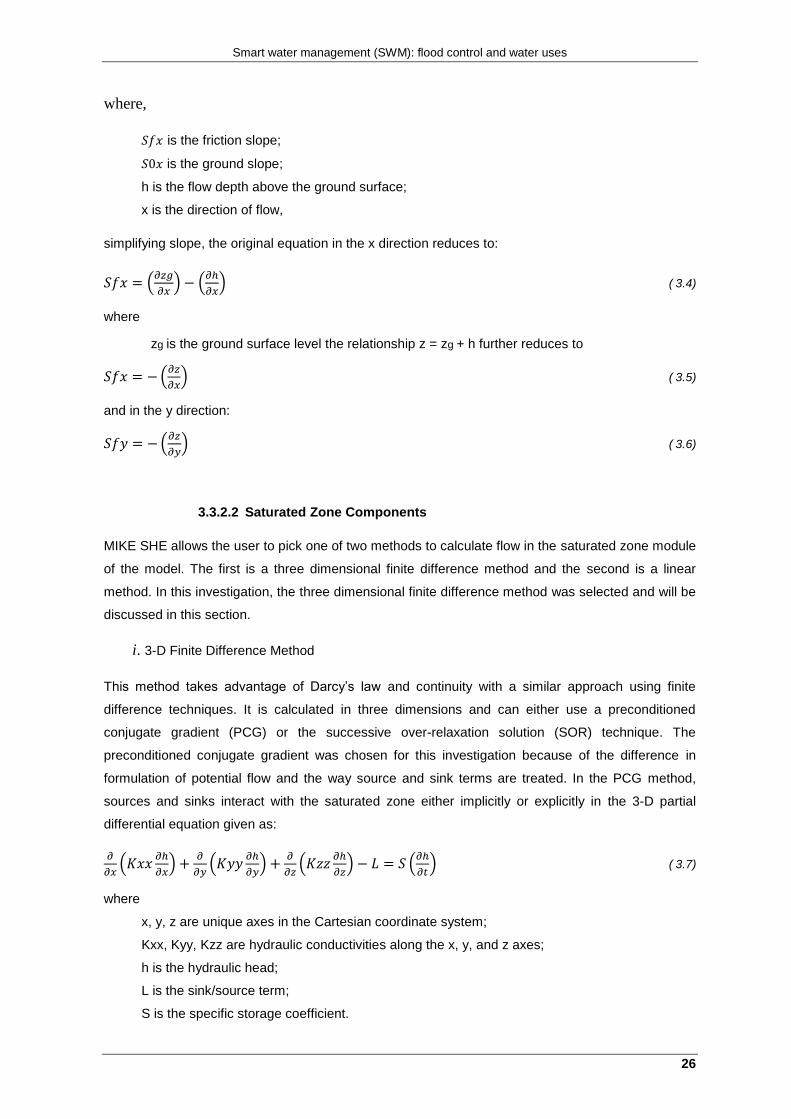
where,
𝑆𝑓𝑥 is the friction slope;
𝑆0𝑥 is the ground slope;
h is the flow depth above the ground surface;
x is the direction of flow,
simplifying slope, the original equation in the x direction reduces to:
𝑆𝑓𝑥 = (𝜕𝑧𝑔
𝜕𝑥) − (
𝜕ℎ
𝜕𝑥) ( 3.4)
where
zg is the ground surface level the relationship z = zg + h further reduces to
𝑆𝑓𝑥 = − (𝜕𝑧
𝜕𝑥) ( 3.5)
and in the y direction:
𝑆𝑓𝑦 = − (𝜕𝑧
𝜕𝑦) ( 3.6)
3.3.2.2 Saturated Zone Components
MIKE SHE allows the user to pick one of two methods to calculate flow in the saturated zone module
of the model. The first is a three dimensional finite difference method and the second is a linear
method. In this investigation, the three dimensional finite difference method was selected and will be
discussed in this section.
i. 3-D Finite Difference Method
This method takes advantage of Darcy’s law and continuity with a similar approach using finite
difference techniques. It is calculated in three dimensions and can either use a preconditioned
conjugate gradient (PCG) or the successive over-relaxation solution (SOR) technique. The
preconditioned conjugate gradient was chosen for this investigation because of the difference in
formulation of potential flow and the way source and sink terms are treated. In the PCG method,
sources and sinks interact with the saturated zone either implicitly or explicitly in the 3-D partial
differential equation given as:
𝜕
𝜕𝑥(𝐾𝑥𝑥
𝜕ℎ
𝜕𝑥) +
𝜕
𝜕𝑦(𝐾𝑦𝑦
𝜕ℎ
𝜕𝑦) +
𝜕
𝜕𝑧(𝐾𝑧𝑧
𝜕ℎ
𝜕𝑧) − 𝐿 = 𝑆 (
𝜕ℎ
𝜕𝑡) ( 3.7)
where
x, y, z are unique axes in the Cartesian coordinate system;
Kxx, Kyy, Kzz are hydraulic conductivities along the x, y, and z axes;
h is the hydraulic head;
L is the sink/source term;
S is the specific storage coefficient.
Smart water management (SWM): flood control and water uses
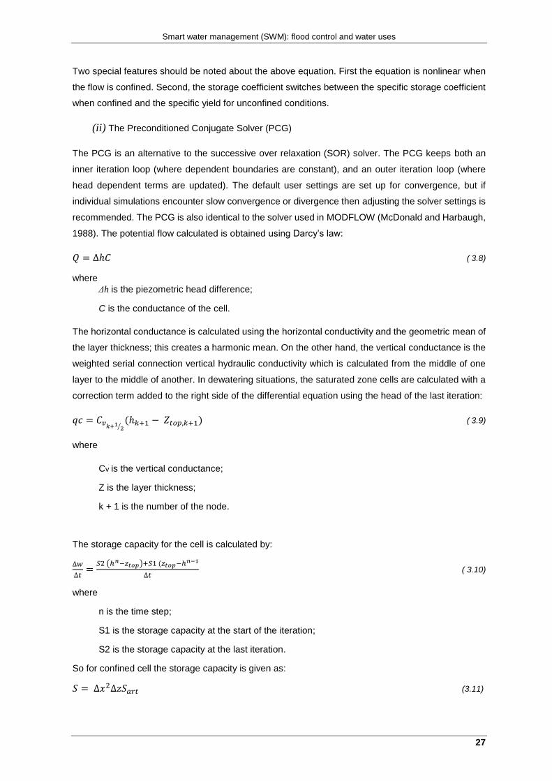
27
Two special features should be noted about the above equation. First the equation is nonlinear when
the flow is confined. Second, the storage coefficient switches between the specific storage coefficient
when confined and the specific yield for unconfined conditions.
(ii) The Preconditioned Conjugate Solver (PCG)
The PCG is an alternative to the successive over relaxation (SOR) solver. The PCG keeps both an
inner iteration loop (where dependent boundaries are constant), and an outer iteration loop (where
head dependent terms are updated). The default user settings are set up for convergence, but if
individual simulations encounter slow convergence or divergence then adjusting the solver settings is
recommended. The PCG is also identical to the solver used in MODFLOW (McDonald and Harbaugh,
1988). The potential flow calculated is obtained using Darcy’s law:
𝑄 = ∆ℎ𝐶 ( 3.8)
where
Δh is the piezometric head difference;
C is the conductance of the cell.
The horizontal conductance is calculated using the horizontal conductivity and the geometric mean of
the layer thickness; this creates a harmonic mean. On the other hand, the vertical conductance is the
weighted serial connection vertical hydraulic conductivity which is calculated from the middle of one
layer to the middle of another. In dewatering situations, the saturated zone cells are calculated with a
correction term added to the right side of the differential equation using the head of the last iteration:
𝑞𝑐 = 𝐶𝑣𝑘+12⁄(ℎ𝑘+1 − 𝑍𝑡𝑜𝑝,𝑘+1) ( 3.9)
where
Cv is the vertical conductance;
Z is the layer thickness;
k + 1 is the number of the node.
The storage capacity for the cell is calculated by:
∆𝑤
∆𝑡=
𝑆2 (ℎ𝑛−𝑧𝑡𝑜𝑝)+𝑆1 (𝑧𝑡𝑜𝑝−ℎ𝑛−1
∆𝑡 ( 3.10)
where
n is the time step;
S1 is the storage capacity at the start of the iteration;
S2 is the storage capacity at the last iteration.
So for confined cell the storage capacity is given as:
𝑆 = ∆𝑥2∆𝑧𝑆𝑎𝑟𝑡 (3.11)
Smart water management (SWM): flood control and water uses
28
where
Sart is storage capacity of the confined cell
and in unconfined aquifers the storage capacity is given as:
𝑆 = ∆𝑥2𝑆𝑓𝑟𝑒𝑒 (3.12)
where
Sfree is the storage capacity of an unconfined cell
Boundaries for this method are the ground surface (upper bound) and the water table (lower bound).
The lower boundary is generally a pressure boundary. The model is set up for hydrostatic initial
conditions (equilibrium, no flow).
Smart water management (SWM): flood control and water uses
29
4. Case study
4.1. Description
Estuaries are especially sensitive to changes since these areas experience different interactions
between multiple forcing factors and ecological systems. Floods in estuaries are associated to
particular climatological conditions, as the coincidence of very high tidal levels and large fresh-water
discharges, or of high tides and storm surge conditions (e.g. spatial distribution of floods in the Tagus
estuary is shown in Figure 4.1). In addition to these progressive phenomena, that are possible to
predict and react, episodes of very intense and concentrated in time rainfall can lead to urban flooding
in areas with insufficient drainage conditions and flash floods in small watersheds tributary to the
estuary. The effects of high water levels in estuaries can be exacerbated by human interventions in
the system, particularly in urban areas where drainage system behavior has to be considered. Rising
sea levels and more extreme climate conditions will increase the vulnerability to inundation of
estuarine margins (Project Molines). At the same time estuaries are ecologically important areas and
anthropic factors such as dense occupation of the estuarine fringe, land reclamation or salt marsh
degradation add complexity to the systems (e.g. Townend and Pethick, 2002; Gedan et al., 2009).
Figure 4.1 - Spatial distribution of database estuarine flood occurrences in the Tagus estuary (Rilo et al., 2015)
4.2. Study area
The Tagus estuary has a high potential to flooding from different sources along its margins, due to the
intense occupation. The estuary is included in the territorial unit of Lisbon and Tagus Valley, involving
18 municipalities in the metropolitan area of Lisbon, for which estimated a population exposed directly
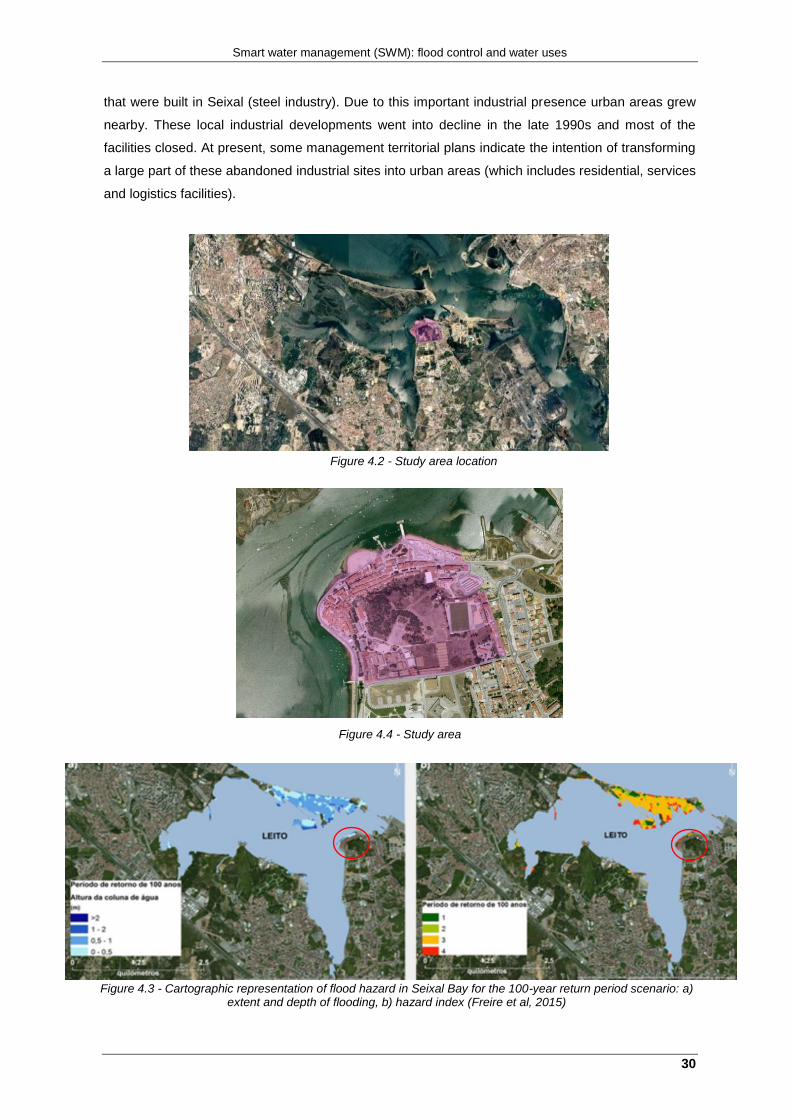
or indirectly of about 2.8 million inhabitants. This study was conducted in a restricted area (Figures
4.2, 4.3, 4.4 and 4.5) located in the southeastern margin of the estuary, that was selected due to past
record of flood episodes and relatively diverse land use occupation, with a total area of 491127m2 and
1170m of margin length. The territorial occupation of this area is associated to relevant industrial sites
Smart water management (SWM): flood control and water uses
30
that were built in Seixal (steel industry). Due to this important industrial presence urban areas grew
nearby. These local industrial developments went into decline in the late 1990s and most of the
facilities closed. At present, some management territorial plans indicate the intention of transforming
a large part of these abandoned industrial sites into urban areas (which includes residential, services
and logistics facilities).
Figure 4.4 - Study area
Figure 4.2 - Study area location
Figure 4.3 - Cartographic representation of flood hazard in Seixal Bay for the 100-year return period scenario: a) extent and depth of flooding, b) hazard index (Freire et al, 2015)
Smart water management (SWM): flood control and water uses
31
Figure 4.5 - Risk index in the Seixal municipality for a 100-year return period scenario (Project Molines)
4.3. The Tagus estuary
As one of the largest estuaries in Europe, the Tagus estuary covers 320 km2, with a deep, long and
narrow tidal inlet linking the Atlantic Ocean to a shallow, tide-dominated basin, with extensive tidal
flats and marshes that cover about 40% of the inner estuary (Figure 4.6 and Table 4.1). About 40 km
upstream, the estuary significantly narrows at the bay head. The saline tide reaches about 50 km
upstream from the mouth, near Vila Franca de Xira. The estuarine bottom is mainly composed of silt
and sand, of both fluvial and local origins; marine sands are confined to the mouth and inlet channel
(Freire et al., 2007).
Table 4.1 - Tagus estuary data
Extension up to the end of the
dynamical tide (Muge) 80 km
Extension up to the limit of salt
water intrusion (VFX) 50 km
Total area (up to VFX) 320 km2
Area between tides 40% of the
total area
Maximum width 15 km
Average width 4 km
Maximum depth 46 m
Average depth 11 m
Length of estuarine margin 360 km
Figure 4.6 - Geometry of Tagus estuary (Project Molines)
Smart water management (SWM): flood control and water uses
32
Tidal ranges vary between 0.55 and 3.86 m in the open coast (Cascais data) but resonance
significantly amplifies the semi-diurnal tidal constituents within the estuary (Fortunato et al., 1999).
Simultaneously, the estuary is strongly ebb-dominated due to the large extent of the tidal flats
(Fortunato et al., 1999).
The average river flow is 368 m3/s (Neves, 2010), and the estuary is usually well mixed. However,
stratification has been observed at high flow rates (Neves, 2010). River discharge may significantly
influence water levels, but only further than 40 km upstream of the mouth (Vargas et al., 2008).
Downstream, the levels are mainly controlled by tide and storm surges. Ocean waves do not penetrate
significantly in the estuary. However, the large extent (fetch) of the estuary allows locally-generated
waves to develop and rework the southern embankment (Freire & Andrade, 1999).
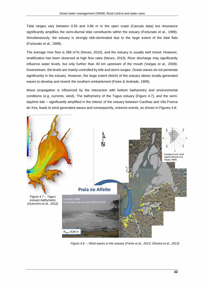
Wave propagation is influenced by the interaction with bottom bathymetry and environmental
conditions (e.g. currents, wind). The bathymetry of the Tagus estuary (Figure 4.7), and the semi-
daytime tide – significantly amplified in the interior of the estuary between Cacilhas and Vila Franca
de Xira, leads to wind generated waves and consequently, extreme events, as shown in Figures 4.8.
Figure 4.7 – Tagus estuary bathymetry
(Guerreiro et al., 2012)
Figure 4.8 – Wind waves in the estuary (Freire et al., 2013; Oliveira et al., 2013)
Smart water management (SWM): flood control and water uses
33
Tidal asymmetry is particularly relevant to sediment dynamics (Aldridge, 1997). Shorter ebbs promote
higher average flow velocities on ebb than on flood because the same volume of water flows in a
shorter period of time. Under those circumstances, the estuary is said to be ebb-dominant. Since the
sediment fluxes depend non-linearly on the velocity, an ebb-dominated estuary will tend to export
sediments. In contrast, a flood-dominant estuary will tend to silt-up more rapidly (Lanzoni & Seminara,
2002).
Studies confirm that the estuary is ebb-dominated in the 40 km reach upstream from the mouth
(Fortunato et al., 1999) and show that it switches to flood-dominated further upstream. The reduction
of the ebb-dominance from km 40 upstream is likely associated to the change in morphology, from a
wide bay with extensive tidal flats to deep and narrow channels. Sea level rise (SLR) will increase the
depth of the estuary, hence reducing the tidal amplitude to depth ratio. As a consequence, flood
dominance should increase. The extent of the tidal flats will decrease, further reducing ebb dominance:
the intertidal area in the Tagus estuary decreases by 40% for a SLR of 1.5 m. In summary, while SLR
will significantly reduce ebb-dominance in the Tagus estuary, sedimentation in the tidal flats will tend
to enhance it. The balance may tend either way, depending on the rate of SLR, the changing
sedimentation rates, and how the marginal areas are allowed to flood. The simulations carried out
show that SLR will have significant effects on estuarine hydrodynamics. In the case of the Tagus they
will be particularly significant due to the occurrence of resonance, which amplifies the semi-diurnal
constituents of the tide. SLR will trigger two major direct effects: Tidal asymmetry will decrease
significantly. The present ebb-dominance will be reduced, and the estuary may even become flood-
dominant. This behavior appears to be mostly due to a significant reduction of the intertidal areas
(roughly 40% for a 1.5 SLR) and will be partly compensated by sedimentation in the tidal flats. And
the resonance within the estuary will be strengthened, increasing the tidal amplification. As a result,
the maximum levels in the estuary will increase slightly faster than the SLR (Guerreiro et al, 2015).
4.4. Extreme water levels
Marginal flooding in the Tagus estuary can have adverse effects. Some urbanized marginal areas,
such as Seixal, are low-lying, so that the potential human and material costs of a flood are high. One
of the most severe historic episodes described was originated by the combination of extreme storm
surge levels and locally generated waves during the February 15, 1941, windstorm, causing high
human casualties and property damages along the estuarine margins (Muir-Wood, 2011).
Recently, the effects of the Xynthia windstorm, that reached the Portuguese coast on February 27,
2010, were also observed along the estuary margins, where significant damages in infrastructures
occurred. In the upper area of the estuary, with extensive agricultural areas, floods may induce
salinization and loss of fertile land. Raising the mean sea level (MSL) implies more frequent floods of
marine origin. In the particular case of the Tagus estuary, this problem will be exacerbated by the
increased tidal amplification due to resonance. The results point out that about 16.1% of the estuarine
Smart water management (SWM): flood control and water uses
34
marginal fringe will be vulnerable to flood for the 2050 scenario, rising up to 23.7% for the 2100
scenario. Urban and industrial areas are the most affected ones in both scenarios: 4.0% and 4.6%
(2050) and 6.0% and 7.8% (2100), respectively. The effects of high water levels in urban areas can
be exacerbated due to the drainage system behavior, which should be prepared for new baseline
conditions. In general, agriculture parcels and green spaces and leisure facilities would be the less
affected sites, given their low representativeness at the study area. However, the Alfeite sand spit, an
important recreational area that also contributes to the maintenance of Seixal bay ecosystem, will be
totally flooded in both scenarios. Vargas et al. (2008), analyzed the vulnerability of the Alfeite spit to
inundation using a combination of hydrodynamic and morphodynamic models under SLR effects and
predicted that in the worst case scenario almost all the spit would be flooded promoting the spit
migration to south. This fact might represent a significant morphological change at the Seixal bay that
can potentially modify the local hydrodynamic behavior leading to a significant change in natural
habitats, Figure 4.9, namely sandy beaches and salt marshes (Guerreiro et al, 2015).
Figure 4.9 - Impact of the urbanization in the tide line, Seixal, (Rilo et al., 2012)
The ongoing rise in sea level affects tidal propagation and circulation in estuaries, and these changes
can have far reaching consequences on the sediment dynamics, water quality and extreme water
levels. The increasing of population is also causing a major impact, the induced erosion may cause
accelerated siltation and the urbanization will increase the runoff. The consequences will be the growth
of water’s turbidity, the acceleration of sedimentation and the spread of silts, muds and clay throughout
the estuary, which leads to a major vulnerability of its margins as shown in Figures 4.10 and 4.11.
Smart water management (SWM): flood control and water uses
49
The above costs are provided as an indicative cost for each type of SUDS. Whilst they provide a range
of costs for each type of techniques used in the case study, the costs associated with any specific site
will depend on a number of factors such as: Scale and size of development; Hydraulic design criteria
(design event, volume of storage required and impermeable catchment area); Inlet/outlet infrastructure
design (volume and velocity of anticipated flows and the capacity of drainage system beyond site
boundary); Water quality design criteria; Soil types (permeability and depth of water table), porosity
and load bearing capacity; Materials availability; Specific utilities requirements; Proximity to receiving
watercourse; Amenity, public education and safety requirements.
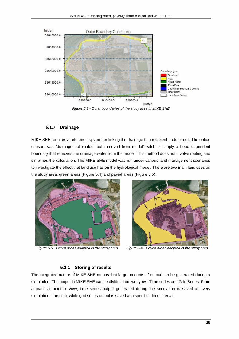
The installation of SUDS in new housing developments will not make a significant contribution to
reducing existing flood risk as these systems are designed to offset the impact of the developments
for a defined pluvial flood event. The ability to retrofit SUDS to existing developments has the potential
to reduce urban water quality and flooding problems through the disconnection of stormwater from the
normal drainage system and installing source control SUDS instead. The methods employed are
similar or the same as those already discussed, but the costs may differ due to the secondary costs
arising from disconnection and transfer of storm water from the existing systems. Previous studies
have assumed that the secondary costs are approximately 20% of the cost of the actual SUDS
construction (SNIFFER, 2006).
6.2.3 Operation and maintenance costs
Sustainable drainage systems require ongoing maintenance to ensure the system remains in good
working order and the design life of the system is extended as long as possible. Operation and
maintenance activities will include: monitoring and post-construction inspection, regular and planned
maintenance and repair maintenance. Costs associated with maintenance will depend on the
frequency of maintenance activities required. These frequencies may be specified by manufacturers
for specific asset types. In the absence of these, the following maintenance items and frequencies
(Table 6.3) have been based on material in the SUDS Manual (CIRIA, 2007).
Table 6.3 - Typical maintenance works and frequencies, CIRIA
Technique Annual or sub annual maintenance Intermittent
Infiltration trench
Monthly - litter and debris removal Annual - weed/root management Annual - removal and washing of exposed stones Annual - removal or sediment from pre-treatment devices
Replacement of filter material (20-25 years)
Detention basin
Monthly - litter and debris removal, grass cutting of landscaped areas Half yearly - grass cutting of meadow grass Annual - manage vegetation including cut of submerged and emergent aquatic plants and bank vegetation cutting
Remove sediment. Repair of erosion or other damage. Repair/rehabilitation of inlets, outlets and overflows
Permeable pavement
4 monthly - brushing and vacuuming
Stabilize and mow contributing areas, removal of weeds. Remedial work to any depressions or broken blocks. Rehabilitation of surface and upper sub-structure where significant clogging occurs. Replacement of filter material (20-25 years).
Smart water management (SWM): flood control and water uses
50
Table 6.4 indicates possible annual maintenance cost ranges, based on a review of literature and
some UK costs, undertaken in 2004 by HR Wallingford.
NEVES, M. 2005. ‘Some suggestions for water management in the Oporto region – in Portuguese, FEUP, Oporto. OECD (2012), Policies to Support Smart Water Systems. Lessons From Countries Experience,
Working Party on Biodiversity, Water and Ecosystems, OECD, Paris, France.
OGDEN, F., Meselhe, E., Niedzialek, J. & Smith, B. 2001. Physics-Based Distributed Rainfall-Runoff
Modeling of Urbanized Areas with CASC2D. Urban Drainage Modeling. American Society of Civil
Engineers.
PENNING-ROWSELL, E. Flood and Coastal Erosion Risk Management: A Manual for Economic
Appraisal.
RAINCYCLE (2005). Rainwater Harvesting Hydraulic Simulation and Whole Life Costing Tool v2.0.
User Manual. SUDS Solutions.
RAMOS, H., Teyssier, C., Energy recovery in SUDS towards smart water grids: A case study.
RAMOS, H., Borga, A. and Simão, M., Cost-effective energy production in water pipe systems:
theoretical analysis for new design solutions. 33rd IAHR Congress. Water Engineering for a
Smart water management (SWM): flood control and water uses
57
Sustainable Environment. Managed by EWRI of ASCE on behalf of IAHR. Vancouver, British
Columbia, Canada, August 9-14, 2009.
RAMOS, H., Covas, D., Pumped-storage solution towards energy efficiency and sustainability:
Portugal contribution and real case studies. Journal of Water Resource and Protection, 2014.
RAMOS, H., Vieira, F., Kenov, K., Environmentally friendly hybrid solutions to improve the energy and
hydraulic efficiency in water supply systems. Energy for Sustainable Development, 2011.
RAMOS, H..; Araujo, L.S.; Coelho, S.T. - Avaliação do desempenho de sistemas em pressão
integrados numa política de gestão sustentável dos recursos hídricos: Caso de estudo. 7º Congresso
da Água – 8 a 12 de Março, Lisboa, 2004.
RAMOS, Helena; 1986, Modelos matemáticos para simulação de escoamentos variáveis em canais.
RAWLINSON, S (2006). Sustainability – Green Roofs. Building Magazine 300606.
Report on the progress in implementation of the Water Framework Directive Programmes of
Measures; Report on the progress in implementation of the Floods Directive
RIBA 2007. Living with water: Visions of a Flooded Future. London: Building Futures.
RILO, A., Fortunato, A., Freire, P. , 2011, Suscetibilidade à inundação de margens estuarinas.
Aplicação à baía do Seixal (estuário do Tejo, Portugal).
RILO, A., Freire, P., Guerreiro, M., Burtorff, A., 2012, Estuarine margins vulnerability to floods for
different sea level rise and human occupation scenarios.
SAHOO, G.B, C. Ray, and E.H. De Carlo. 2006. Calibration and validation of a physically distributed
hydrological model, MIKE SHE, to predict streamflow at high frequency in a flashy mountainous Hawaii
stream. Journal of Contaminant Hydrology. In Press.
SANTOS, F. D; Miranda, P. (2006). Alterações Climáticas em Portugal: Cenários, Impactos e Medidas
de Adaptação. Projecto SIAM II. Lisboa, Gradiva.
SANTOS, R. (2011), Inundações urbanas e medidas construtivas para a sua mitigação, Dissertação
para obtenção do Grau de Mestre em Engenharia Civil, Instituto Superior Técnico.
SCHOLZ, M. & Kazemi Yazdi, S. 2008. Treatment of Road Runoff by a Combined Storm Water
Treatment, Detention and Infiltration System. Water, Air, and Soil Pollution.
SINGH, R., K. Subramanian, and J.C. Refsgaard. 1999. Hydrological modeling of a small watershed
using MIKE SHE for irrigation planning. Agricultural Water Management.
SNIFFER (2006). Retrofitting Sustainable Urban Water Solutions. Final Report, Project UE3(05)UW5.