SÉMINAIRE DE PROBABILITÉS (STRASBOURG)

DAVID J. ALDOUS

Random walks on finite groups and rapidlymixing Markov chains

Séminaire de probabilités (Strasbourg), tome 17 (1983), p. 243-297.

<http://www.numdam.org/item?id=SPS_1983__17__243_0>

© Springer-Verlag, Berlin Heidelberg New York, 1983, tous droits réservés.

L’accès aux archives du séminaire de probabilités (Strasbourg) (http://www-irma.u-strasbg.fr/irma/semproba/index.shtml), implique l’accord avec les conditions gé-nérales d’utilisation (http://www.numdam.org/legal.php). Toute utilisation commer-ciale ou impression systématique est constitutive d’une infraction pénale. Toutecopie ou impression de ce fichier doit contenir la présente mention de copyright.

Article numérisé dans le cadre du programmeNumérisation de documents anciens mathématiques

http://www.numdam.org/

RANDOM WALKS ON FINITE GROUPS AND RAPIDLY MIXING MARKOV CHAINS

by

David Aldous*

Department of StatisticsUniversity of California at Berkeley

1. Introduction

This paper is an expository account of some probabilistic techniques

which are useful in studying certain finite Markov chains, and in particular

random walks on finite groups. Although the type of problems we consider

and the form of our results are perhaps slightly novel, the mathematical

ideas are mostly easy and known: our purpose is to make them well-known!

We study two types of problems.

(A) Elementary theory says that under mild conditions the distribution

of a Markov chain converges to the stationary distribution. Consider the

(imprecise) question: how long does it take until the distribution is close

to the stationary distribution? One might try to answer this using

classical asymptotic theory, but we shall argue in Section 3 that this

answers the wrong question. Instead, we propose that the concept "time until

the distribution is close to stationary" should be formalized by a parameter

T, defined at (3.3). Since it is seldom possible to express distributions

of a chain at time t in tractable form, it is seldom possible to get T

exactly, but often T can be estimated by the coupling technique. One

situation where these problems arise naturally is in random card-shuffling,

where T can be interpreted as the number of random shuffles of a particular

kind needed to make a new deck well-shuffled. In Section 4 we illustrate

the coupling technique by analysing several card-shuffling schemes.

(B) Some chains have what we call the "rapid mixing" property: for a

random walk on a group G, this is the property that T is small comparedto #G, the size of the group. When this property holds, probabilistic

techniques give simple yet widely-applicable estimates for hitting time*

’

Research supported by National Science Foundation Grant MCS80-02698.

244

distributions. These are discussed in Section 7. The fundamental result

(7.1) (7.18) is that for a rapidly mixing random walk with uniform initial

distribution, the first hitting time on a single state is approximately

exponentially distributed with mean R#G. Here R, defined at (6.4), is a

parameter which can be interpreted as the mean number of visits to the

initial state in the short term. This result, and its analogue for rapidly

mixing Markov chains, has partial extensions to more complicated problems

involving hitting times on arbitrary sets of states, and hitting times from

arbitrary initial distributions.

This paper is about approximations, which may puzzle the reader: since

for finite Markov chains there are of course exact expressions for distri-

butions at time t and hitting time distributions in terms of the transition

matrix. However, we have in mind the case where the state space is large,

e.g., 52! in the case of card-shuffling. Exact results in terms of 52! x52!

matrices are seldom illuminating.

In principle, and sometimes in practice, random walks on groups can be

studied using group representation theory, the analogue of the familiar

Fourier theory in the real-valued case. Diaconis (1982) studies convergence

to stationarity, and Letac (1981) studies hitting times, using this theory.

Our arguments use only the Markov property; we are, so to speak, throwing

away the special random walk structure. So naturally our’results applied to

a particular random walk give less precise information than can be obtained

from the analytic study of that random walk, if such a study is feasible.

Instead, our results reveal some general properties, such as exponential

approximations for hitting times, which are not apparent from ad hoc analyses

of particular cases.

Finally, we should point out two limitations of our techniques. To

apply the Markov chain results it is usually necessary to know the stationary

distribution, at least approximately: one reason for concentrating on random

walk examples is that then the stationary distribution is uniform. Second,

the rapid mixing property on which our hitting time results depend seems

characteristic of complicated "high-dimensional" processes, rather than the

245

elementary one-dimensional examples of Markov chains, for which our techniques

give no useful information.

2. Notation

The general case we shall consider is that of a continuous-time

irreducible Markov process (Xt) on a finite state space G = {i,j,k,...}.

Let Q(I ,j ), j # I , be the transition rates, qi - ~ #. Q(i,j), and let’

j~

p..(t) = be the transition probabilities. By classical theory

there exists a unique stationary distribution ir, and

(2.1 ) pi ~j(t) ~~(j) as

(2.2) X = j)--~~r(j) a.s. as t-~~ ,

twhere timeSit: Xs =j) = is the random variable measuring the

amount of time before time t spent in state j.

The same results hold for a discrete-time chain (X ), except that for

the analogue of (2.1) we need aperiodicity:

(2.3) as provided X is aperiodic.

In Section 3 we study convergence to stationarity in the continuous-time

setting; the results hold in the discrete-time aperiodic setting with no

essential changes.

Given a discrete-time chain (X ) with transition matrix P(i,j) we can

define a corresponding continuous-time process (X*) with transition rates

= P(i,j), j # i. In fact we can represent explicitly as

(2.4) Xt = XN t

where Nt is a Poisson counting process of rate 1.

Let TA (resp. TA) be the first hitting time of X (resp. X*) on a set A

from some initial distribution. Then TA = by (2.4), and it is easyA

to see

(2.5) 1 as TA ~ ~ , °

In Section 7 we study hitting time distributions for continuous-time processes;

246

by (2.5) our results extend to discrete-time chains. It is important to

realise that even though the results in Section 7 use rapid mixing, they may

be used for periodic discrete-time chains by the observation (2.5) above,

since it is only required that the corresponding continuous-time process

be rapid mixing.

We shall illustrate our results by discussing the special case of random

walks on finite groups. Suppose G has a group structure, under the opera-

tion ®. Let p be a probability measure on G such that

(2.6) support(p) generates G.

The discrete-time random walk on G associated with p is the process

Xn+1 = Xn ® ~n+1 , where (~n) are independent with distribution p.

Equivalently, Xn is the Markov chain with transition matrix of the special

form

P(iJ) = u(i 1 ® J) . .

By (2.6) the chain is irreducible. The stationary distribution is the uniform

distribution TI(i) = 1/#G. As at (2.4) there is a corresponding continuous-

time random walk (Xt), and it is for this process that our general results

are stated, although in the examples we usually remain with the more natural

discrete-time random walks. The results in the general Markov case become

simpler to state when specialized to the random walk case, because of the

"symmetry" properties of the random walk. For example, ETITi’ the mean

first hitting time on i from the stationary distribution, is clearly not

dependent on i in the random walk case.

When stating the specializations in the random walk case we shall assume

(2.7) qi = 1 .

This is automatic if p assigns probability zero to the identity; otherwise

we need only change time scale by a constant factor to attain (2.7).

We shall avoid occasional uninteresting complications by assuming

247

(2.8) max i 03C0(i) ~ 1 2,which in the random walk case is merely the assumption that G is not the

trivial group.

We should make explicit our definition of hitting times:

TA = min{t >0:

as distinct from the first return times

(2.9) T~ - min{t>0:

Elementary theory gives

(2.10)

where we are using the convention a/bc = a/(bc).

For sequences (a ), (b ) of reals,

a - bn means lim = 1 ;

bn means lim sup an/bn ~ . .

Finally, the total variation distance between two probability measures on

G is

= max 1 .

AGG "- ’

3. The time to approach stationarity

In the general Markov case write

(3.1) di(t) = -~rN

for the total variation distance between the stationary distribution and the

distribution at time t for the process started at i. Let

d(t) = max d.(t) .i

’

248

Note that in the random walk case d.(t) does not depend on i, by symmetry,

so d(t) = di(t). In general the elementary limit theorem (2.1) implies

d ( t ) --~ 0 as

Moreover, classical Perron-Frobenius theory gives

d(t) - as some C>0, 0~1 . .

(In discrete time, a is the largest absolute value, excepting 1, of the

eigenvalues of the transition matrix.) Thus a describes the asymptotic

speed of convergence to stationarity. However, in our examples of rapidly

mixing random walks the function d(t) looks qualitatively like

That is, d(t) makes a fairly abrupt switch from near 1 to near 0. It seems

natural to use the time of this switch rather than the asymptotic behaviour

of d(t) to express the idea of "the time taken to approach uniformity".

Informally, think of this switch occurring at a time T. Formally, define

(3.2) T(e) = min{t:

(3.3) T = T(1/2e)

where the constant 1/2e is used merely for algebraic convenience; replacing

it by a different constant would merely alter other numerical constants in

the sequel.

249

The idea that d(t) makes an "abrupt switch" can be formalized by

considering a sequence of processes. For example, in applying a particular

shuffling scheme to an N-card deck we will get functions dN(t), TN(~).In some examples we can prove (and we believe it holds rather generally)

that there exist constants aN such that

(3.4) a N as for each 0e1 . .

In other words, the scaled total variation distance function dN(t/aN)converges to the step function for t 1 1. An example is shown in

Fig. 3.24.

The next lemma gives some elementary properties of d(t), which can

probably be traced back to Doeblin.

(3.5) LEMMA. Define

03C1i,j(t) = ~Pi(Xt ~.) - Pj(Xt ~.)~ ; 03C1(t) = max 03C1i,j(t) .

Then (a) 2d(t).

(b) p is submultiplicative : p(S+t) p(s)p(t).

(c) d(t) is decreasing.

Proof. Assertion (a) follows from the triangle inequality for the total

variation distance. The other assertions can be proved algebraically, but

the proof is more transparent when coupling ideas are used. The key idea is

the following fact, whose proof is easy.

(3.6) LEMMA. Let Z1, Z2 have dis tributions vl, v2. Then

°

Conversely, given vl, v2, we can construct such that

IIvl-v211 = P(Zl ~ Z2) ;

Zn has distribution vn ( n =1, 2 ) .

To prove (b), fix i., , i , s, t. Construct (Z1,Z2) such that

250

Z" has the distribution of X~ given X~=i~ ;(s).

s s 1’2

Then on the sets A. = construct such that

Z1s+t = Z2s+t

And on the sets Aj,k = {Z1s = j, Z2s = k} (j ~ k) construct (Z1s+t,Z2s+t) such

that

~.t~-~j~ = ~’t~ ’ ~~t~-!’j~ = ’kCt~-) ~

~~ ~~t~~t!~,k)=~j~’

~ pd) .

Now Z~ . (resp. Z~.) has the distribution of X~ given Xo = i~ (resp. i~),and so

by (3.7)

ip(t)p(s) .

To prove (c), use the same construction except for giving Z~ ~ the

stationary distribution and having =

d~ (s). Then

d,

This result is useful because it shows that an upper bound on p at a parti-

cular time t.. gives an upper bound for later times:

p(t) i

Translating this into an expression involving t explicitly,

p(t)i(p(tQ))~~0-~ .In particular the definition (3.3) of T makes and we obtain

the following bound, which we shall use extensively.

251

(3.8) COROLLARY. d(t) exp(1 - t/T) , t ~ 0.

REMARKS. (a) We are here stating results for continuous time; the same

results hold in the discrete time aperiodic case.

(b) Note that the exponential rate of convergence in finite state

processes is a simple consequence of the basic limit theorem (2.1). The

Perron-Frobenius theory is only needed if one wants an expression for the

asymptotic exponent.

(c) Corollary 3.8 can be rephrased as

T(E) T(1 0 e 1 .

As mentioned in the Introduction, it is seldom possible to get useful

exact expressions for p..(t), and hence for d(t) or r(E:). We shall

instead discuss how to get bounds. The basic way to get lower bounds on

d(t) and T(e) is to use the obvious inequality

d(t) ’_ I

for some A C G for which the right side may be conveniently estimated.

We should however mention another general method which gives effortless,

though usually rather weak, lower bounds. Recall that the entropy of a

distribution p is ent(p) = log u(i). In particular, the uniform

distribution n on G has ent(Tr) = log #G. We quote two straightforward

lemmas.

LEMMA. Let (X ) be the discrete-time random walk associated with u, and

let p be the distribution of Xn. lhen n

LEMMA. If v is a distribution on G such that e then

ent(v) > (1-e) log #G.

From these lemmas we immediately obtain the lower bounds

(3.9) > ; 03C4(~) ~ (1-~) log #G ent( )for discrete-time random walks.

252

Our next topic is the coupling method, which is a widely-applicable

method of getting upper bounds on T. We remark that for the applications

later to hitting time distributions we need only upper bounds on T; and

often rather crude upper bounds will suffice.

Let (Xt) be a Markov process. Fix states i, j. Suppose we can

construct a pair of processes such that

(3.10) Z~ (resp. Z2) is distributed as X given i (resp. j);

(3.11) Z1 - Z2 on {t > T} , where

T (= T~’J) = inf{t:

Call (Zl,Z2) a coupling, and T a coupling time. By Lemma 3.6

(3.12) P(T’~>t) . °

Thus from estimates of the tails of the distributions of coupling times we

can get estimates for d(t). A crude way is to take expectations. Suppose

we have constructed couplingsfor each pair i, j. Then

(3.13) where T = max

~ ~ 1 ,J

because by (3.12) p(t)

To summarize: to get good estimates of the time taken for the process

to approach stationarity, we seek to construct couplings for which the

coupling time is as small as possible.

We now outline the strategy we shall use in constructing couplings. It

is conceptually simpler to discuss the discrete-time case first. Suppose

we have a function f: GXG-~{0,1,2,...} such that f(i,j) = 0 iff i = j:

call f a distance function. Suppose that for each pair (i,j) there is

a joint distribution

6.. = such that

(3.14) ~

JC(V) = Pd,’); C(M) = P(j,-); V=W if i=j.

253

Then we can construct the bivariate Markov process (Z1,Z2) such that

P((Z1n+1,Z2n+1)~.|(Z1n,Z2n) = (i,j)) = 03B8i,j .This is plainly a coupling. Think of the process D = as measuring

the distance between the two processes; the coupling time is

T = min(n: Dn = 0) .

All our couplings will be of this Markovian form. To specify the coupling,

we need only specify the "one-step" distributions 6... Of course there

will be many possible choices for these joint distributions with prescribed

marginals: since our aim is to make Dn decrease it is natural to choose

the distribution (V,M) to minimize Ef(V,M), and indeed it is often

possible to arrange that f(V,W) f(i,j) with some positive probability of

a strict decrease. Once the coupling is specified, estimating the coupling

time (and hence T) is just estimating the time for the integer-valued

process Dn to hit 0. Note, however, that Dn need not be Markov.

In the continuous-time setting, we merely replace the joint transition

probabilities by joint transition rates i,j(k,l) such that

(3.15) 03A3 i,j(k,l) =

Q(i,k) ; 03A3 i,j(k,l) = Q(j,l) ; i,i(k,k) = Q(i,k) . ’

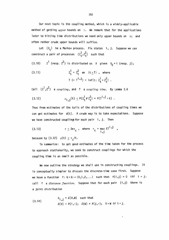
We should mention the useful trick of time-reversal. Suppose (X ) is

the random walk associated with p. Let p*(j) = u(j-1). Then the random

walk associated with p* is called the time-reversed process, because

of the easily-established properties

(a)

(b) when XD and X~ are given the uniform distribution,

(X~,X~,...,XK) ~ (X K ,X K-1 ,...,X ) . 0 °

The next lemma shows that when estimating d(n) we may replace the originalrandom walk with its time-reversal, if this is more convenient to work with.

(3.16) LEMMA. Le t d(n) fresp. d*( n ) ) be the total variation function fora random walk Xn (resp. the time-reversed walk X*n) . Then d(n) = d*(n). °

254

Proof. Writing i for the identity of G,

I

- ~ ~ Pj_1 (Xn = i ) -1/#G~ I by the random wal k property

= = i ) -1/#G~ I re-ordering the sumJ

j n

= 03A3|Pi(X*n = j) - 1/#G| by (a)

= d*(n) .

Of course it may happen that p = ~*, so the reversed process is the

same as the original process: call such a random walk reversible. In the

general continuous-time Markov setting, a process is reversible if it

satisfies the equivalent conditions

(3.17)~(~)p>>j(t) =

Although we lose the opportunity of taking advantage of our trick, reversible

processes do have some regularity properties not necessarily possessed by

non-reversible processes. For instance, another way to formalize the concept

of "the time to approach stationarity" is to consider the random walk with

X~ = i and consider stopping times S such that XS is uniform; let Tibe the infimum of E.S over all such stopping times, and let T = min Ti.It can be shown that T is equivalent to r for reversible processes, in

the following sense.

(3.18) PROPOSITION. There exist constants C1, C2 such that T C2Tfor all reversible Markov processes.

This and other results on reversible processes are given in Aldous (1982a).

The rest of this section is devoted to one example, in which there is

an exact analytic expression for d(t) which can be compared with coupling

estimates.

(3.19) EXAMPLE. Random on the N-dimensionaZ cube. The vertices of the

255

unit cube in N dimensions can be labelled as N-tuples i = (il,...,iN) of

0’s and 1’s, and form a group G under componentwise addition modulo 2.

There is a natural distance function f(i,j) = Write

0 = (0,...,0), (0,...,0,1,0,...,0) with 1 at coordinate r,

1 ~ r ~ N ,

p(j) = 0 otherwise.

The random walk associated with p is the natural "simple random walk" on

the cube, which jumps from a vertex to one of the neighboring vertices

chosen uniformly at random. The discrete-time random walk is periodic: we

shall consider the continuous-time process, though similar results would

hold for the discrete-time random walk modified to become aperiodic by

putting

= 1/(N+1) 1 r N= 1/(N+l)

We now describe a coupling, which will give an upper bound for T. Fix

i, j; let L = f(i,j) and let C = be the set of coordinates

c for which jc ~ i. . Define as follows.

= 1/N , c ~ C.

(if L>1) ll.. i ® ® 1 N 1

(interpret cL+1 as c1).(if L = 1 ) A..(i = = c E C.

Let be the associated coupling, i.e. the Markov process with tran-

sition rates It is plain that the distance process Dt = evolves as the Markov process on {O,l,...,N} with transition rates

Q(n,n-2) = n/N (2 n N), Q(1,0) = 2/N. It is not hard to deduce that the

coupling time T is stochastically dominated by the sum

T* = T*1 + T*3 + T*5 + ... + T*M ; M = N (N odd) ,

N-1 (N even),

256

where the summands are independent exponential random variables, T* m having -

mean N/m. To estimate the tail of the distribution of T* we calculate

ET* = N(1 +1/3+1/5+... +1/M) ~ ~! 1og(N)var(T*) = +(1/3)~ + ... +(1/M)~) -

So ~-,d(aN P(T*>aN 1og(N))

2014~0 as by Chebyshev’s inequality.

So we conclude

r(e) ~ 1og(N) ; 1 0 e 1 .

Me shall now show how to get an exact analytic formula for d(t). Write

the continuous-time random walk X. componentwise as (X’..,X’j. It is

easy to verify that the component processes are independent Markov

processes on {0,1} with transition rates Q(0,’!) = Q(1,0) = 1/N. So the

component processes have transition probabilities

Po(X~=0) =~{-!+exp(-2t/N)} , Po~"~ =~{1-exp(-2t/N)} .So the transition probabilities for the random walk are

(3.20) = 2’~{1 L = f(j,0) .

Thus we obtain the formula

(3.21) d(t) = 2~ ~ N .

L=0 ’-

Elementary but tedious calculus shows -

(3.22) lim 1og(N)) = 1 , t 1N "

= 0 , t > 1 ,

and hence

(3.23) r(e) - ~ 1og(N) , 0 e 1.

257

Thus we see that the upper bound for T derived by the coupling technique

gives the correct order of magnitude, though not the correct constant, in

this example.

Figure 3.24 shows computer-c,alculated graphs of d( t / log N) for

N = 8, 32, 128, 512, to illustrate the convergence in (3.22).

REMARK. Our use of total variation distance to measure how close a distribu-

tion is to the stationary distribution may seem an arbitrary choice. What if

we used another indicator, say entropy? In this example the entropy ~(t)of the distribution of Xt has the form

~(t) = Ncp(t/N)

for a certain Thus CPN(e) does not exhibit the "abrupt switch" of

for large N. So it is hard to see how to define a parameter analogous

to T in terms of entropy; and it is not clear that the hitting time approxi-

mations of Section 7 would be valid under some definition of "rapid mixing"which used entropy rather than total variation distance.

258

4. Card-shuffling models

Imagine a deck of N cards, labelled 1 to N. The state of the deck may

be described by a permutation ’n- of {1,...,N}, the card labelled i being

in position where position 1 is the top of the deck and position N

the bottom. So the card in position j is labelled A shuffle of

the deck may also be described by a permutation a, indicating that the

card at position i has moved to position 0(1). A probability distribution

p on the group GN of permutations describes the random shuffle in which

o is picked according to the distribution p. Write Xn(i) for the

position of the card labelled i after n independent such random shuffles.

Then Xn = (Xn(i)) is the random walk on the group GN associated with u.

Let n be the uniform distribution on GN. Imagine starting with a

new deck (i.e. with the card labelled i in position i). As in section 3

let d(n) be the total variation distance between the distribution of Xnand n. Think of the parameter T at (3.3) as measuring the number of

shuffles needed to get the deck well-shuffled. Our purpose in this section

is to estimate T for some specific shuffles p. More precisely, we shall

try to find the asymptotic behaviour of TN as the number of cards N tends

to infinity. We shall get upper bounds by coupling. To describe couplings,

we imagine two decks, in states ~r, a, say, and then specify dependent

random shuffles of the two decks, each Er having distribution ~.

The joint distribution 6 of is the transition matrix for

the coupled processes. One way of getting lower bounds is to consider the

motion of a particular card: this motion Yn = Xn(i), i fixed, forms the

Markov chain on {1,...,N} with transition matrix

(4.1) P(j,k) = b

the stationary distribution is uniform. Writing dy for the total variation

distance function for y , we have the obvious inequality

(4.2) d(n) > dy(n) .

We shall need three famous results from elementary probability theory,

259

which we now describe.

Given two decks, say a match occurs.whenever one position is occupied

by the same labelled card in both decks. Let {i : be

the number of matches between decks in states -n- and a. Then

(Feller (1968) p. 107)

(4.3) CARD-MATCHING LEMMA. For X uniform on (1)

as N

Note that f(7r,a) = the number of unmatched cards, is a natural 1

distance function on GN.Second, let Rn be the number of distinct cards obtained in n

uniform random draws with replacement from the deck. That is,

~n = #{C1,...,Cn}, where Ci are 1.1.d. uniform on {1,...,N}. Let

Lj = min{n: Rn =N-j}

be the number of draws needed to get all but some j cards. Then from

Feller (1968) pp. 225 and 239

(4.4) COUPON-COLLECTORS LEMMA. If 0 a 1 and if j = j(N) satisfies

0 1im 00, then 1-a zn In

for fixed j we have 1 in probabi Zi ty.

Third, consider again random draws with replacement, and let U be

the number of the first draw on which we obtain some previously-drawn card:

U = mi n {n : Cn = C i for some i n } .

(4.5) BIRTHDAY LEMMA. U/N 1/2 -+ V V, where 0 V ~.

We now describe and analyse some examples. Several of these are in

Diaconis (1982).

(4.6) EXAMPLE. "Top to random". Here we shuffle by removing the top card

and replacing it in a random position in the deck. For a formal description,

for 1 j . N define the permutation 03C0j by

260

’~~ ( i ) = i -1 , i j= i , i > j.

Then the random shuffle is rr , for J uniform on {1,...,N}. We shall

prove

(4.7) T(E) N N loq(N) ; 0e1 . .

To analyse this example it is convenient to use the time-reversed process,

as discussed in section 3. Here, the time-reversed process is "random to

top". That is, a card is chosen uniformly at random, and moved to the top

of the deck. To construct a coupling, consider two decks. Choose a label

C uniformly from {1,...,N} and in each deck move the card labelled C

to the top. Plainly this is a coupling. The coupling time T is the time

at which the decks are completely matched. Now matches, once created, are

not destroyed, so at the time La at which each label has been chosen at

least once, the decks are completely matched. So

By the Coupon-Collectors Lemma,

(4.8) d(aN as a > 1.

To get the lower bound, consider the set A. J of states ~r for which

the bottom j cards have increasing labels: that is,

1f-l(N-j+l) 1f-l(N-j+2) ... Suppose we start with a new deck.

Let L. be the number of shuffles until all but some j labels have been

chosen. If L. > n then the bottom j cards after n "random to top"

shuffles have never been chosen to be moved, so remain in their original

relative order with increasing labels. So P(Xn E Aj) > Since

= 1/ j ! ,

d(n) - > P(L. J >n) - l/j! .

Using the Coupon-Collectors Lemma, we find

261

d(aN 1 as N--~~ ; a l.

This and (4.8) establish (4.7).

In the example above the coupling is very simple. And in fact the

upper bound could be obtained without using coupling, by observing that the

order of the already-chosen cards in "random to top" shuffling is uniform.

But here is a minor modification for which the coupling argument is equally

trivial but where a direct argument seems hard. Diaconis (1982) records that

Borel proposed this shuffle.

(4.9) EXAMPLE. "Top to random, bottom to random". Here we alternate between

picking the top and the bottom card to be removed and replaced at random.

Again we get

T(e) - N log(N) ; 0 e 1,

using the obvious modifications of the arguments above (for the lower bound,

consider the set of states for which some j successive cards have

increasing labels).

(4.10) EXAMPLE. "Transposing neighbours". Here we pick at random a pair of

adjacent cards, and transpose them. To eliminate periodicity, we also allow

the possibility of doing nothing. Formally, let Tr be the identity

permutation, and 03C0j the permutation transposing j and j+1. Then the

random shuffle for J uniform on {0,...,N-1}. We shall prove

(4.11) T j

for constants Cl, C2.We need first some results about the motion (Yn) of a single card

under this shuffle. This motion is the Markov chain on {1,...,N} with

transitions

= = 1/N

P(j,j) = 1 - 2/N

P(1,1 ) = P(N,N) = 1 -1/N .

262

This is a symmetric random walk with reflecting boundaries. It is a

straightforward exercise in weak convergence theory to show that, suitably

normalised, this converges weakly to Brownian motion Bt on [0,1] with

reflecting boundaries:

N-1Y[2t/N3] ~ Bt .

The first assertion of the lemma below is now immediate, and the second is

not hard.

(4.12) LEMMA. Let S.. be the number of shuffles until the card initially

at the top reaches the position (i.e. the middle). ~hen

S 1 /N3 2 V, where V > 0.

Let 52 be the number of shuffles until the card in an arbitrary initial

position reaches the bottom. Then there exist constants K, S > 0, such

that

s O. N>1.

Suppose Yo = 1, and write dy(n) for the total variation distance between

the distribution of Yn and uniform. Then

_[N/2J) - CNl2JlNI I

~ 1 > n) -1 2and so

by the first assertion of Lemma 4.12. For small a the right is greater

than 1/2e, and so we get the lower bound T > aN .To get the upper bound, suppose we can produce a coupling (Xl,X2) with

the following two properties.

(a) Matches are not destroyed. That is, if X~(i) = X~(i) then

X~(i) = X2(i) for m > n.

(b) A card in one deck cannot jump over the same card in the other deck.

That is, if (resp. ) X2(i) then X~(i) ~ (resp. ) X2(i)

263

for n > 0.

Given such a coupling, the coupling time is T = max Ti’ where Ti is the ’

time until the cards labelled i are matched. But by (b) we have S2,the number of shuffles for the card labelled i to reach the bottom of the

deck (in the deck where this card is initially higher). So

log(N))

NKe-03B2C log(N) by Lemma 3.10

- -~ 0 provided C > 1/P,

and then T ~ CN3log(N).To exhibit a coupling satisfying (a) and (b), consider two decks in

states ~r, o. Let S be the set of j such that neither the cards in

position j are matched nor the cards in position j+1 are matched. List

S as {jl,...,jL} and add to S. Let J be uniform on

{0,...,N-1} and define J* by

J* = J if J f S= if J = jkES (interpreting as jo).

The coupling is produced by applying shuffle 03C0J to the first deck and 03C0J*to the second deck. This is a coupling, because J* is uniform. Property

(a) is immediate. And the only way in which (b) could fail is if the same

transposition 03C0j were applied to both decks when the card at position jin one deck had the same label as the card at position j+1 in the other

deck: and the coupling is designed so this cannot happen.

REMARKS. (a) This shuffle generates a reversible random walk.

(b) The lower bound obtained by considering entropy (3.9) gives T > CNin this example, which is rather crude.

(4.13) EXAMPLE. "Random transpos itions". Here we shuffle by transposing a

randomly chosen pair of cards. To avoid periodicity, we again allow the

pair to be identical. For the formal description, let 7r.. be theJl,J2

permutation transposing jl and j2. Then the shuffle is , where

264

J1 and J2 are independent, uniform on {1,...,N}. We shall prove

(4.14) ~N T ~ CN~ ; for some constant C.

Diaconis and Shahshahani (1981) use group representation techniques to

analyse this shuffle. From their results one can obtain the precise result

(4.15) T(E:) - ~I 2 1og(N) ; 0 E 1 .

To describe the coupling, note that the random shuffle may be described

as: pick a label C and a position J at random (independent, uniform),

and then transpose the card labelled C with the card at position J. Given

two decks in states 77, a, pick C and J and shuffle each deck as

described above. Plainly this is a coupling: let (Yl,Y2) be the states

of the decks after this shuffle. Then Y1(C) = Y2(C) = J. Thus we see

(a) if neither the cards labelled C were matched, nor the cards at

position J were matched, in the decks fr, a, then ,at least one

new match has been created, so M(Yl,Y2) > M(~,a) + 1;(b) otherwise the number of matches remains the same, M(Yl,Y2) =

Now the chance that the event in (a) happens is where

= is the number of unmatched cards. Let (Z1,Z2) be the

coupled process, and D = the number of unmatched cards in the

coupled process. By (a) and (b), the process Dn is stochastically dominated

by the Markov process Dn on ~0,1,...,N} with transition matrix

P(iJ-1) = (ilN)2 ; P(i,i) =

So the coupling time T is at most the first passage time T* of D~ from

N to 0. So

(N/i)2 CN2 ,i=1

and (3.13) gives the upper bound in (4.14).

To get the lower bound, suppose we start with a new deck (state ~D,

say). Let L. be the number of shuffles needed until the j last card has

265

been picked. By the Coupon-Collectors Lemma, recalling that two cards are

picked on each shuffle,

(4.16) P(L_>aN1og(N))-~1 ; a~. .Let A. J be the set of states -n- for which #{i: - > j. Then

if So

d(n) > P(XnEAj) - where X is uniform on GN- > P(L. J > n) - >j)

and (4.16) and the Card-Matching Lemma give

d(aN 1og(N)) --~ 1 ; a ~- . .

This establishes the lower bound in (4.14).

REMARKS. (a) This shuffle also is reversible.

(b) For this example the lower bound (3.9) obtained from entropy

considerations is T > CN.

(4.17) EXAMPLE. "Uniform riffle". We now want to model the riffle shuffle,

which is the way card-players actually shuffle cards: by cutting the deck

into two roughly equal piles, taking one pile in each hand, and merging the

two piles into one. If the top pile has L cards, this gives a permutation

7T such that

(4.18) ~r(2) ... and ~r(L+2) ... ~(N) .

Call a shuffle satisfying (4.18) for some L a riffle shuffle. Such a

shuffle can alternatively be described by a 0-1 valued sequence (b(1),...,b(N)),where b(j) = 0 (resp. 1) indicates that the card at position j after the

shuffle came from the top (resp. bottom) pile: formally,

~r(1) = min{j: b(j) =0}

7T(i) = b(j) =0} , i L = #{j: b(j) =0}

7r(L+1) = min{j: b(j)=l}

L+1 1 i N .

266

To model a random riffle shuffle we specify some probability measure p on

the set R of riffles. The easiest way is to take p uniform on R. In

terms of the second description, this means we take (B(1),...,B(N)) to be

independent, P(B(i) = 1) = P(B(i) = 0) = 1 2. Call this the uniform riffle.

This process has been investigated in detail by Reeds (1982) (see also

Diaconis (1982)), whose technique we shall use to prove

(4.19) 3 2log2N , 0 e 1 .

In actual riffle shuffles, successive cards tend to come from alternate

piles: see Diaconis (1982), Epstein (1977) for discussion. A more realistic

model would be to take (B(i), 1 ~i ~N) to be Markov, with transition

matrix P(0,1) = P(1,0) = e, say (Epstein suggests e = 8/9). The only

result known for this model is the lower bound given by entropy (3.9): for

fixed e,

as N--~~ ,

where &#x26;(e) = -e 1og28 -(1-e)log2(1-6). It is natural to conjecture

T(e) - C03B8log2N as N-+oo (e, e fixed) .

But the argument we shall use for the uniform riffle (8 = ~) 2 does not extend

to general 6, for which no reasonable upper bound is known.

The uniform riffle is another example for which it is easier to analyse

the time-reversed process. This reversed shuffle can be described as follows.

For each c write on the card labelled c the number Bl(c), where

(B1(c): are independent as before; form one pile consisting of the

cards with 0 written on them, in their original order, thereby leaving

another pile of cards with 1 written on them; and place the first pile on top

of the second pile. Imagine now doing this reverse shuffle again with

independent numbers B2(c); this will produce a deck with a sequence of

cards on top which have (Bl,B2) _ (0,0), followed by a sequence with

(1,0), followed by (0,1), followed by (1,1). Continuing, after n

reverse shuffles let D (c) = n 2m-1B (C), and then

267

(4.20a) the random variables (D (c): are independent, uniform

on {0, ... ,2n-1 } >

(4.20b) the order of the deck is such that Dn is increasing, and cards

with identical values of Dn are in their original relative order.

We shall now use this description to get bounds on the total variation

distance d(n). We first present a coupling argument for a crude upper bound.

Consider two decks, and apply the reverse shuffle to each using the same

(Bm(c)). Let Fn be the event that the numbers (Dn(c): are

distinct. Then the coupling time T satisfies T n on Fn, by (b). So

d(n) 1 - P(Fn). But the Birthday Lemma shows that P(Fn) -~1 1 when

in such a way that N/(2n)1/2~0, Hence d(a for a > 2,

which gives the crude upper bound 2 log2N.We turn now to the lower bound. For a deck in state Tr let be

the number of adjacent pairs of cards with increasing labels:

e(-rr) = #{j:

where a. J is the indicator function of Consider

first X uniform on GN. Then the random variables even (resp.

odd)} are independent, and we easily get

(4.21) , Ee(X) = (N-1)/2 ; var 6(X) N/2 .

Now imagine starting with a new deck, and performing n reverse shuffles,

leaving the deck in state X. Since D has at most 2n distinct values,

(b) implies e(Xn) > N - 2n. From this and (4.21) we can immediately get

T(e) N > log2N. However, a slightly more delicate analysis will improve this

bound. We first quote a straightforward variation of the Birthday Lemma.

(4.22) LEMMA. Let (Ci) ) be independent, uniform on ~1,...,M}. Let

UN = #{n N : Cn = C; for some i n } , If M - Na for some a > 1

then

EUM - ~I 1 2-a , , var(UM) - ~I 1 2-a .

268

Let If and M -- Na. for

some 03B1 > 3/2 then EVN ~ 0.Recall Xn is the state of the deck after n reverse shuffles. Let

Jn be the (random) set of positions j for which the cards at positions

j and j+1 after the shuffles have the same value of D :

Jn = {j: D n (X n 1(j))=D n (X n 1(j+1))} .Then, conditional on Jn,

(i) ;

(n) the random variables even (resp. odd)} are independent.

From this we can calculate

(4.23) (N-1)/2 + ~#J ; Now by (a) the distribution of #Jn is the same as the distribution of UNin Lemma 4.22, for M = 2n. So, putting

for some’!a?.Lemma 4.22 gives

* ~ S=2-a1 . .

So using (4.23)

(4.24) E6(X ) _ (N-1)/2 + v Nl/2 ; where var 8(X ) N/2 .

Chebyshev’s inequality applied to (4.21) and (4.24) gives

p(6(X) > (N-1)/2+~v Nl/2) -~ 0p(e(X ) > (N-1 )/2 +~ N1/2) -1 1

and so d (n) 1 , giving the lower bound in (4.19).

We shall now return to the upper bound. Fix a > 3, 2 n = 1 +[a log2N],so 2n > Na. Let X be the state of the deck, described at (4.20), after

269

n reverse shuffles starting with a new deck. The random variables

(D~(c) = 1 c N) define a random partition A. of the shuffled deck into

sets consisting of the positions of cards with common values of Dn- Thus if

the numbers Dn(c) are (15,2,8,15,15,2), then when put in increasing order,

they become (2,2,8,15,15,15), and this defines the partition {1,2}, {3},

{4,5,6}. Denote a partition by A = {A-.,A?,...}, and let lAir be the

number of sets with exactly r elements in the partition A. Let P be

the set of partitions consisting only of singletons and consecutive pairs.

Using Lemma 4.22

(4.25) E~A~ 2~ NZ°~’ as

(4.26) 1 as

And by conditioning on the set of distinct values taken by (Dn(c): 1 ~c N),we obtain

(4.27) for AEP the probability P(Ar= A) depends only on

Now for m > 0 let Wl,...,Wm be i.i.d. uniform on {1,...,N-1}, and let

A* be the collection of sets 1 j m. If these sets are

disjoint, extend A*m to a partition by including the remaining elements of

{1,...,N} as singletons. Given that A~ is such a partition, it is plainly

distributed uniformly over the partitions A ~ P with = m. So by

(4.27)

(4.28) A E P) = is a partition)

t P(A,m = A) , A E P .

Now let ~r be a state of the deck, and as before let e(7r) be the

number of successive pairs with increasing labels. Say a partition

A = {Al,A2,...} is consistent with ~r if 1 is increasing on each A..

Fix y, S such that y > > 2 > S > 2-a, y+S 1. J

(4.29) LEMMA. P(A~ is some partition consistent ~r) >

(1 2)m{1 - 03C8(03B8(03C0) - N/2 N03B3,m N03B2,N)}

270

where

PROOF. Given that the pairs are disjoint and

that 7T’ is increasing on each, there are at least e(’rr)-3(i-1) choices

for M. which have ’IT-1 increasing on and {W..M.+1} disjoint

from the previous pairs. So

P(A* is some partition consistent with ir) > n {03B8(03C0)-3(i-1) N-1}> (1 2)m {1 + 2xN03B3-1 - 6iN-1} , where x = 03B8(03C0) - N/2." "

1=1 N~

Calculus shows the product tends to 1 as x2014~0,

Me can express the distribution of X n

by conditioning on the partition

~ using description (4.20), as

N.P(X,=.)=~=A)(2!) !AL ’(3.) )AL ’"~(A consistent with.)!A!.

1(A consistent with ’IT)

= P(A~P( 03A3P(|A|2 = m|a~P)2m 03A3P(A=A||A|2 = m, A~P)

. (A consistent with ’IT)

(4.30) ~ P(~P)P(|A|2 = m|~P)(1-03C8(03B8(03C0)-N/2 N03B3,m N03B2,N)) ,

by (4.28) and Lemma 4.29.

By (.4.21) we can find such that the set F.. of states ’IT

such that |03B8(03C0) - N/2 N03B3| ~ ~N satisfies #FN/N! ~ 1.By (4.25) we can find such that Applying

these observations and (4.26) to (4.30) we obtain

N!P(X=-rr)~1-B., where ~N~~’

So the total variation distance d(n) between X n

and the uniform distribu-

tion satisfies d(n) ~ X..+(1 -M~-)2014~0, establishing the upper bound in

(4.19).

271

(4.31) EXAMPLE. "Overhand shuffle". Here is an example of a random shuffle

for which no good upper bound for T is known. Overhand shuffling is where

the deck is divided into a number of blocks, and the order of the blocks is

reversed. To make a model, let 2 K N/2 be a parameter which will

represent the mean length of the blocks. Let (Vi: N) be independent,

P(Vi = 1) = 1/K, and let V~ = VN = 1. Let

J1 - 0 ; Ji 1 = min{j > Ji-1: Vj = 1} ; {j: Ji j Ji+1 ~ .

Then B. represents the ith block, and the random shuffle is:

7T(j) = (N-Ji+1 ) + (j-Ji ) ~ I j

The only result known is the following lower bound, whose proof we shall

merely indicate. -

T > C max(K,(N/K) ) ; some constant C .

Note that the right side is minimized by K = N2/3, for which T > CN2/3.First, consider two cards which are initially adjacent. On each shuffle,

the chance they are separated is at most 2/K, and this leads to the

inequality T - > CK. Second, consider the motion Yn of a particular card

after n shuffles, where we measure its position from the top for even n

and from the bottom for odd n. Then Yn is a Markov process on ~1,...,N}

which, away from 1 and N, is approximately a random walk whose increments

have mean 0 and standard deviation 21/2K. It can be shown that Y hasn

standard deviation at most CKn1/2, and this leads to the other inequality.

.REMARK. One would like to conjecture that for any "reasonable" way of shuffling

cards, T is at most polynomial in N. But it is not clear what "reasonable"

means. Note that for our applications to hitting times, we only need T

small compared to N!

5. Rapidly mixing Markov chains

In this section we mention a few Markov chain examples, and discuss

informally the "rapid mixing" property.

272

(5.1) EXAMPLE. "Ehrenfest urn model". We discuss the continuous-time version,

which is the Markov process Yt on ~0,1,...,N} with transition rates

- Q(i,i+1) = 1 - ilN , Q(i,i-1) = i/N .

Think of N balls distributed among two boxes, with a Poisson (rate 1)

process of selections of balls chosen uniformly at random and transferred to

the other box; Yt describes the number of balls in a particular box at

time t. Now we can represent Yt as where Xt is the random walk

on the N-dimensional cube (Example 3.19), and f(i1,...,iN) = In fact,

the random walk describes the process of balls in boxes where the balls are

labelled 1,...,N, and state i = (il,...,iN) indicates that ball r is

in box i .

r

From this representation we see that the stationary distribution -n-

for Y is the Binomial (N,~-) distribution. And d(t) is the same for

Y as for X, so

(5.2) T(~) ~ ~I 4 log(N)

by (3.23).

(5.3) EXAMPLE. "Random subsets". Let 1 M N, N > 3, and let B be

the set of all subsets B of {1,2,...,N} with #B = M. Consider a random

subset B evolving by elements being deleted and replaced by outside

elements. Formally, consider the B-valued process Xt with transition rates

Q(B,B’) = ~ = M-1 1

=0 ; other B’ ~ B.

The stationary distribution is uniform on B. The reader may like to

construct a coupling argument similar to that of Example 3.19 to show

(5.4) T CN log(1 + min(M,N-M)) as for some constant C.

(5.5) EXAMPLE. "Sequences in coin-tossing". Let (~i) be independent,

= H) = 1/2, 1 =T) = 1/2, representing repeated tosses of a fair

273

coin. For fixed N > 1 the process Xn = (~n+1’’.’’~n+N) is a Markovchain on For this chain the stationary distribution is uniform and

(5.6) d(n) = 1 - (~)N n , ’ 0 n N

=0 , n ~ N.

(5.7) EXAMPLE. "Random walk in a d-dimensional box". We want to consider

the random walk on the d-dimensional integers restricted to a box of side

N by boundaries. Formally, let G = {i = (il,...,id) : 0 ir N} and consider

the Markov chain with transition matrix

P(i,j) = 1/(2d+1) for 1;

= 0 for other j ~ i;

P(i,i) = 1 - ~ P(i,j) ..# .

(We use 1/(2d+1) instead of 1/2d to avoid periodicity problems.) The

stationary distribution is uniform, and using the Central Limit Theorem we

see

(5.8) T - CdN2 as for fixed d.

(5.9) EXAMPLE. cube". One may consider the random walk on Rubic’s

cube obtained by choosing one of the 27 possible rotations at random at each

step. It would be interesting to estimate T for this random walk. Perhapsone of the algorithms to "solve" (i.e. reach a specific state of) the cube

could be used to construct a coupling. But this seems difficult.

We now introduce informally the "rapid mixing" proeprty. For a discrete-

time random walk, this is the property

(5.10) T is small compared to #G .

The intuitive idea here is that the distribution of the chain approaches

stationarity while only a small proportion of states have been visited. For

the general discrete-time chain, we measure "proportion of states" using the

stationary distribution, and so formulate the rapid mixing property as

274

(5.11) T is small compared to

For continuous-time processes we must take into account the rate at which

transitions occur. Recall q. = L Q(i,j) is the rate of leaving state i.’

j1iIn the general Markov case the rapid mixing property becomes

(5.12) T is small compared to

Recall (2.7) that in the random walk case we normalize to make q. 1 = 1, so

then (5.12) is the same as (5.10).

Almost all the examples mentioned have this rapid mixing property.

It is particularly noticeable in the card-shuffling examples, where #G = N!

but T is at most polynomial in N. An exception is the random walk in the

d-dimensional box for d = 1 or 2. Indeed, it is easy to see that the familiar

examples of l-dimensional Markov processes do not have the rapid ’mixing

property. For instance, consider the single server queue process on

{0,’!,...,N}, with transition rates

Q(iJ-1) = 1 ; Q(i,i+1) = a 1 ;

and stationary distribution = a~(1-~)/(1-~N+1). Very roughly, T must

be of the same order as the passage time from N to 0, which is of order

N/(1-a): to put it another way, the process starting at N must pass

through most states before approaching the stationary distribution.

We thus have a curious paradox: the rapid mixing property, which we use

in the sequel to get approximations for hitting times, seems characteristic

of complicated high-dimensional processes rather than simple one-dimensional

processes. A possible explanation is that rapid mixing is a kind of "local

transience" property, and we recall that mean zero random walks are transient

only in three or more dimensions. This analogy is pursued a little in the

next section.

6. The mean occupation function

In this section we discuss the mean occupation function Ri(t), which

275

plays a major role in the behaviour of rapidly mixing Markov processes. For

a Markov process (X ) and a state i define

t(6.1) R~(t) = 0 p..(s)ds

where time(s t: is the random variable indicating the amount of

time X spends at state 1 before time t.

In the next paragraph we describe informally the behaviour of Ri(t) in

a rapidly mixing process: the rest of the section contains lemmas formalizing

these assertions.

The function R.(t) looks roughly like

That is, R.(t) initially tends to increase to a value which must be at

least 1/q., the mean length of the initial sojourn in i (6.2). It then

starts to level off, and remains essentially constant over the interval of

t large compared to T but small compared to (6.5). So we can

define a parameter R; as the approximate value of Ri(t) on this interval.

Interpret Ri as the mean length of time (mean number of visits, in the

random walk case) spent at i in the short term. For another interpretation,

recall that in the infinite state space setting the condition is

equivalent to transience, and then = 1/qi(1-pi), where p. is the

probability of return to i. Analogously, in the rapid mixing case we may

think of R. as approximately where p* is the probability

276

of return to i in the short term (6.17). In particular, if is close

to 0 then Ri is close to 1/q.. Finally, note that in the random walk

case Ri and Ri(t) are quantities R and R(t) not dependent on i.

We now start the formalities. First, Pi ’ - > e-qis, so

(6.2) Ri(t) ~ t0 e-qis ds = q-1i(1-e-qit) .

Second, by integrating the inequality d(s) we get, for

ti i t2’

(6.3) ~ Ri (t2) - Ri (tl ) - (t2-tl )~r(i ) ~ I d(s)ds

2. T exp(1-tl/T) by (3.8).

So the limit

(6.4) R. = lim ~ t-+oo’

exists and is finite. This quantity occurs in the traditional analytic

treatment of Markov process theory; one reason for its significance will

become clear in the next section. To compute Ri directly would require

knowing p..(t), which is rarely available explicitly in practice. But

by (6.3) we see

(6.5)

If t is large compared to T then the second term on the right is small;

if t is small compared to i then the first term on the right is

small compared to 1/q.; in the rapidly mixing case we can find t satis-

fying both these conditions and then R.(t) approximates R.. This is the

informal description of R. 1 given earlier. Specifically, from (6.5) we get

(6.6) for T(1 - log

in general; and in the random walk case

(6.7) ~R- R(T*) I 2T*/#G ; for T* = T(1 + log #G) .

277

In Section 8 we shall see examples where R is estimated in this way.

Our informal discussion earlier suggested that for rapidly mixing

processes, R. should not be much smaller than 1/q.. Lemma 6.8 formalizes

this idea. To state such a result we introduce a notational device, to be

used extensively in the next section. Call a function ~(x) > 0, x > 0

vanishing if ~(x) -~ 0 as x --~0, and adopt the convention that a function

asserted to be vanishing is a "universal" function, that is to say the function

does not depend on the particular process under consideration. The symbol

~ will denote different functions in different assertions.

(6.8) LEMMA. Ri + q.T))}, for some vanishing &#x26;.

Specializing to the random walk case,

(6.9) R ~ 1 -V~(#Glog(1+T)) .Results like this could equivalently be formulated as limit theorems for

sequences of processes. For instance, Lemma 6.8 is equivalent to:

Let X be processes on state spaces G; let in E Gn; suppose

q~

then Rnin > .

Both formulations have the same interpretation:

If 7r(i) is small compared to 1/q.r log(1+qiT) then R.is not much less than 1/q..

The formulation involving vanishing functions seems to convey this idea more

directly.

PROOF OF LEMMA 6.8. By (6.2) and (6.5)

(6.10)

We want to evaluate this at a time t0 which is large compared to T log(1+q.T)

278

but small compared to To do so, define

(6.11) a =

t0 = 03B1-1/203C4 log(1+qi03C4) = 03B11/2/qi03C0(i) .

Note that d(t) ~ e-qit - 1 2 by assumption (2.8), so the

definition of T gives

(6.12) = -log(1 2 + 1 2e) > 0 .

Evaluating (6.10) at t = to’

(6.13) .

Now each of the functions

1og(1+c))

(6.14) 03B11/2

sup y>0

is a vanishing function of a, and the result follows.

We remark that for non-rapidly mixing processes there is the weaker

lower bound

(6.15) Ri ~ 1 2qiwhich cannot be improved: see Section 7. Of course for non-rapidly mixing

processes, Ri does not have the intuitive meaning described earlier. We

also remark that for reversible processes (6.15) can be improved. In a

reversible process the function is decreasing (in fact, completely

monotone: Keilson (1979)). So

t

R. i =

~ t00{e 1 -03C0(i)}ds , where e 1 = Tr(i)

(6.16) (Xt reversible).

279

Let F. , be the distribution function of the first return to i:

F. (t) = Pi(T+i ~ t) .(6.17) ) LEMMA. ~Riqi(1 - Fi(T )) - 1~ ~(1_F. T* ) ) ~here ~ is vanishing

and T* = T(1 -log

In other words, for rapidly mixing processes we can approximate Ri by

1/qi(1-Fi(T*)), as discussed informally earlier.

As a preliminary, we need

(6.18) LEMMA, (a) qiRi(t) ~ 1 1-Fi(t)(b) (1-e n) 1 1-{Fi(t)}n+1 1-Fi(t), n _ > 1.

PROOF. Let X - i. Let [U ,V ) be the nth sojourn interval at i. Then

~t)

= 03A3 q-1iP(Un~t)

~ q-1i 03A3 P(Um-Um-1~t; 1m~n)

= qi1 L ~ n>1

- q lfl - F.(t)} _ l, giving (a).

To prove (b),

n+1

~ E(Z An) L ~ t, 1 r m)

where Z has exponential (1) distribution, .

= ( 1_e_n ) ~ n+1 {Fi(t)} m_1 , giving (b).m=1

PROOF OF LEMMA 6.17. By Lemma 6.18(a) and (6.6),

1

280

giving one side of the inequality. For the other, write a = 1

and let n be the integer part of

a 1/2(1-F~ (’r*) ) 1 - a~(q~d))-’’ . .Note n > for some vanishing Setting t - n(T* + 1/q.),Lemma 6.18(b) gives

(1 - (1-e n)(1 - >(6.19)

1 ()

using the fact that {~(a)}’ 1 for some vanishing ~. Finally,

by (6.5) 61 + 82, say, where

81 = a

82 =

q.T*e exp(-nT*/T)°

which with (6.19) establishes the lower bound in Lemma 6.17.

Lemma 6.17 implies that if the process started at i is unlikely to

return in the short term, then Ri should be about 1/q.. Our final two

lemmas in this section give upper bounds in this situation. The first is

applicable if the transition rates into i from other states are all small.

(6.20) LEMMA. q.R. 1 +,~(a), where a = and

q* = max q 0 ..J~i ~’ 1

PROOF. Set t - a 1/2 Tlog(1+q.T), so and

Since the rate of return to i is at most q*, we have q*t. By

Lemma 6.18(a),

q.R.(t ) (1_q*t )-1 1 (1_al/2)-1 1 i 1 + 03C8(03B1) .i i 2 (l-q 2 ~ (l-a ) ~ 1 + W a .

And by (6.5)

281

qiT t2/T)_ al/2 + ~,(a) ,

The final lemma is applicable when there is a distance function f

such that f(Xt,i) tends to increase away from Xo = i.

(6.21) LEMMA. Let f be a distance function on G. Let 0 s 1.

Suppose c is a constant such that for each j # i,

c a k: I k~j

Then 0 t (1-s)/c.

PROOF. Fix i. Consider the process

f(X(tAT.),i) °

’

The definition of c ensures that Yt is a supermartingale. So for j ~ i,

s. But f(X(t^T.),i) = 0 on {T~ t}, so

This ies

Hence F.(t) s+ct, and the result follows from Lemma 6.18(a).

7. Hitting times

Mean hitting times EiTj, and more generally hitting distributions,have been studied for many years, but there is no single method which yieldstractable results in all cases. Kemeny and Snell (1959) give elementarymatrix results; Kemperman (1961) presents an array of classical analytic

techniques. Our purpose is to give approximations which are applicable to

rapidly mixing processes. Keilson (1979) gives a different style of

approximation which seems applicable to different classes of processes.

We first give two well-known exact results, which concern the case of

hitting a single state from the stationary initial distribution.

282

(7.1 ) PROPOSITION.

In the random walk case, = R#G.

(7.2) PROPOSITION.

Proposition 7.1 is useful because it shows we can estimate by

estimating Ri.. Proposition 7.2 is less useful, because estimating Fi(y)in practice may be hard. We shall give "probabilistic" proofs, quoting

renewal theory. First, a lemma about reward renewal processes. Informally,

if you are paid random amounts of money after random time intervals, then

your long-term average income per unit time should be

E(money paid per interval)/E(duration of interval).

(7.3) LEMMA. Let (Vn,Wn), n > l, be positive random variables. Let~ ~ ~

n n

Z(t) be an increasing process such that Z(~ 1 Vi) _ ~ 1 Wi’(a) If (Vn,Wn), n > 1, are i.i.d. and EVl = v, EW1 = w, then

lim = w/v a.s.

(b) Suppose sup EW2 ~, sup EVZ ~, and there exist constantsn n

v, w such that > v, w for aZZ n,

where ~ - Q(V ,W ; m n). Then lim inf > w/v a.s.n m m -

-

PROOF. In case (a), the strong law of large numbers says that a.s.

Vn = n-103A3Vi ~ v , Wn = Vn+1-Vn ~ 0 ,

and the result follows easily. In case (b) we can use the strong law for

square-integrable martingales (Stout (1974) Theorem 3.3.1) to show that a.s.

lim sup Vn v , ,lim inf Wn > w , ~ 0 ,

and again the result follows easily.

PROOF OF PROPOSITION J.1. Fix i, tl > 0, let p(.) =

1 E .) and let

U1 - min{t: i } .

283

Let Yn be the block of X over the interval that is,

YS =

X~ +S , 0 s °

The blocks (Yn), n > 1, are i.i.d. So we can apply Lemma 6.3(a) to

Vn = Un+1 _ Un

Wn = t i me ( s : Un+1, i )

Z(t) = time(s: Ul s t, Xs = i )

and the lemma shows

(7.4) lim = EV1/EW1 a.s.

Now EV1 - R.(t ), t 1Z(t) _ 03C0(i). Substitutinginto (7.4) and rearranging,

(7.5) > EpTi - {Ri (tl ) - 03C0(i)t1 }/03C0(i) .

Letti ng tl ~ ~, we have ~ 0, so E03C1Ti ~ E03C0Ti, and the resul t

follows.

PROOF OF PROPOSITION 7.2. Let XO = i. Let SO = 0,

S - time of nth return to i

Y(t) = min{Sn-t: Sn > t} .Then Y ( t ) has distribution (Ti E .), where pt

= E .). So

Y(t) ~ P (T. E . ) as

But are the epochs of a renewal process with inter-renewal

d i s tributi on E.), and for such a process (Karlin and Taylor (1915))

we have

Y(t) -~-~ Y ,

where P(YEdy) = Pi(T> The result follows from (2.10).

We can deduce a useful lower bound.

284

(7.6) COROLLARY. 1 ~(2q~(i))~ . .

PROOF. Fix c > 0. Consider the class C of distributions on [0,oo)

which have a decreasing density f(t) with f(0) = c. The distribution in

C with minimal mean is plainly the distribution uniform on [O,c 1]. So

every distribution in C has mean at least (2c)" . The result now follows

from Proposition 7.2.

In view of Proposition 7.1, the Corollary is equivalent to

(7.7) Ri > 1/2qi .

Inequalities (7.6) and (7.7) cannot be improved, even for the random walk

case: consider the cyclic motion Q(0,1) = Q(1,2) = ... = Q(N-1,N) = Q(N,0)

- l. Of course, in the rapidly mixing case R. is essentially at least

1/qi by Lemma 6.8.

We now start the approximation results. The first says that for

rapidly mixing processes the exact value of the mean hitting time

on i from the stationary distribution is an approximate upper bound for

the mean hitting time from an arbitrary initial distribution.

(7.8) PROPOSITION. For any state i and any initial distribution v,

where ~ is vanishing.

In the random walk case, this says i + ~(T/#G)}. In words, when

T is small compared to #G then the mean hitting time on a state from any

other state cannot be much more than R#G.

We need the following lemma.

(7.9) LEMMA. Fix t, pi = Then

max t + max

PROOF. First recall 1

285

(7.10) max E j T A .J

So

(7.11 ) > E Pi TA E03C0TA + d ( t) max But obviously EiTA t + ETA (giving the first inequality), so

max EiTA max by (7.10). Rearranging,

max

i i A - ~r A

Substituting into (7.11) gives the second inequality.

PROOF OF PROPOSITION 7.8. By Lemma 7.9,

1- 1

+ >( d(t)) (1 t > 0 .I

So by Proposition 7.1 and Corollary 7.6,

, t > 0 .

Evaluating the right side at t large compared to T, small compared to

we see from (3.8) that the right side is at most 1

Consider for fixed i how the mean hitting times vary with j.

Proposition 7.1 says that the 03C0-average of these hitting times is

Proposition 7.8 says that.each E.T. is not much more than these

imply that EjTi must be approximately equal to for j.

It is straightforward to formalize and prove such a result: let us just

state the random walk case.

( 7.12 ) COROLLARY. ~’here is a vanishing function ~ such that for random

walksE.T.

#ljt I > e} e#G , for ~ = V~(T/#G) .

So rapidly mixing processes have the property that is almost constant,

over most j. It can be shown that for reversible processes this property

is actually equivalent to rapid mixing, see Aldous (1982a).

286

Of course one cannot expect to have EjTi approximately equal to

for aZZ j, since there will often be states j such that the

process started at j is likely to hit i quickly.

We now consider the time to hit subsets of states, rather than single

states. Here even approximations are hard to find: let us give some lower

bounds on the mean time to hit a subset from the stationary initial distribution.

(7.13) PROPOSITION. Suppose qi ~ 1. Then

(a)

(b) E T > min R..~A 1 - log(1+T) )}, where ~ is vanishing.~r A - ~EA

i

PROOF. (a) By (2.5) it suffices to prove this for a discrete-time chain.

There, n) EA) _ ~r(A), and so n) Let

N = Then N

’- ~ n=1

N

> ~(1 -n~r(A))1

= N - 1 2N(N+1 )03C0(A)

- 1 03C0(A) - 1 - 1 2 1 03C0(A) (1 03C0(A) + 1)03C0(A)

giving (a).

The proof of (b) is similar to the proofs of Lemma 6.8 and Proposition

7.1. Analogously to the latter proof, fix tl and set

Ul - min{t: Xt ~ A}Un = mi n {t > Un-1+tl : Xt E A}

. vn - Un+1 - Un

Wn = time{s: Un s Un+1, Xs E~A}

Z(t) = time{s: Ul s t, Xs EA}

Fn = o( Xs : s Un+1 )pi(.) = Pi(Xt E.) . .

287

Then

max Ep.TA

Also Wn ~ t1; and max 2 because the state space is finite, so

max EV2 oo. So we can apply Lemma 7.3(b) to obtainn

n

7r(A) = 1im

Estimating v(t,) by Lemma 7.9 and rearranging,

(7.14)

We want to evaluate this at a time t, large compared to T log(1+T) but

small compared to So set

a = ir(A)T log(1+T)

t1 = a-1/2T log(l+T) = a1/2/n(A) .

Then, setting w = min R~,iEA

I + by (6.5)

~

and since w 2 > > by (7.7),

w(t )(7.15) ~ w - 1~ ~{a) .Also = a 1/2 /w

(7.16)

And by (3.8), Putting this, (7.16) and (7.15) into (7.14}gives the result.

In the rapidly mixing random walk case, Proposition 7.13 gives anapproximate lower bound of R#G/#A for E7TTA. If the subset A is "sparse"

288

in the sense that, starting at one element of A, the random walk is unlikely

to hit any different element of A in the short term, then this lower bound

is approximately the correct value of Such a result can be proved by

the techniques of Proposition 7.13: but since the conditions are hard to

check in practice, we shall merely state one form of this idea.

(7.17) PROPOSITION. There is a vanishing function 03C8 such that for randomwalks

#A - ~ 03C8(

#A +

where bA = max +2log #G)).

We shall now discuss the distribution of hitting times TA. At first

sight, the difficulty of estimating the mean for general A suggests

that one could say little about the distribution. But it turns out that,

in the rapidly mixing case, the hitting time distribution on A from a

stationary initial distribution is approximately exponential, provided 7r(A)

is sufficiently small.

(7.18) PROPOSITION. There is a vanishing function ~ such that

sup In other words, the distribution is approximately exponential provided E7TTAis large compared to T. In the random walk case, it is sufficient by

Proposition 7.13 that #A be small compared to #G/T. In particular, our

informal definition of "rapid mixing" (5.10) ensures that in a rapidly mixing

random walk the exponential approximation for the hitting time on a single

state will I be valid.

Proposition 7.18 is proved in Aldous (1982b), and we will not repeat

the details. The main idea is that the conditional distributions

Bh = must stay dose to ~r, because the tendency of vtto drift away from 7r (due to paths hitting A being eliminated) is

counteracted by the rapid mixing. So = (T A > s) is

289

approximately P,~(TA >s), and this makes TA be close to exponential.

We now discuss the distribution of TA for rapidly mixing processes

when the initial distribution v is arbitrary: our remarks are formalized

in Proposition 7.19 below. There is a certain probability p, say, that

the process hits A in the short term (compared to Given this does

not happen, the distribution of TA is approximately exponential, mean

In other words, the Pv-distribution of will be a mixture of a

distribution concentrated near 0 (with weight p) and a distribution close

to the exponential mean 1 distribution (with weight 1-p). So is

approximately So assuming is known, estimates of either

p or give estimates of the other.

Of course if p is close to l, these arguments tell us only that

EvTA is small compared to

( 7.19 ) PROPOSITION. For arbitrary v, A, Zet m = m = There

is a vanishing function ~ such that

sup > t) - m xp(-t/m) ~ I E

t>Em v m -

where ~ _

Analogously to (7.12), when A is a "small" subset in a rapidly mixing

process, then will be close to for "most" j, and so for

"most" j the Pj-distribution of TA will be approximately exponential.

PROOF OF PROPOSITION 7.19. Set a = T/m, and suppose a 1. Set

J = {j: P.(T t ) al/3} . °We assert

(7.20)

Indeed, by definition of J we have, for j ~ J,

Xnt0 = j ) 1 - al/3

290

and so P (min(T.,T.) >nt~) ~ (1-a~~)", giving

t~a’~ = a~~m .

Next we assert

(7.21) jej,

For , setting p, = P.(X. e.),

!P.(T.>t)-P (TA > t-t0)| ~ by definition of J;j ~ P~ ~ u 2014

~~(a) by (3.8);

~~(a) by Proposition 7.18;

= c~ .

Next, set tp = and let B be the event For

t ~t~,~~A’~-~A~’~~~A~~J~)

by (7.20)

(7.22) ~(a) .

And for t ~ t?,

mm P,(T.>t) P (TA > t|B) ~ max P,(T.>t-t.) ,

so from (7.21)

!P~(T~ > t ~(a) + t~/m~ ~(a) ; t ~ t~ .

Using (7.22),

(7.23)

It remains to estimate P(B). First,

t~+mmax ../. B by Lemma 7.9

(7.24)

291

Second, note the elementary inequality

(7.25)

Now for j E J and p = 0 G .

by (7.25)

~ d(t0) + 03B11/3

and so by (7.24)

> m(1-~V(a)) ; j E J .

Using (7.24) again,

(7.26)

Now from the definition of B,

. P(B) min EjTA ETAIB P(B){max

Combining this fact with (7.26),

(7.27)

Now 03A9 is covered by where

B~ = B2 =

So we estimate the contribution to the expectation of TA made over these

sets.

E03BDTAlB1 EiTA)

E.Tj by the argument for (7.22)

~ 03C8(03B1)m using (7.24)

E03BDTAlB2 ~ t2 = 03B11/4m .

292

Combining these with (7.27),

This estimate for P(B), substituted into (7.23), establishes the

Proposition.

REMARK. By applying Proposition 7.19 to the distribution v of the position

after the first jump out of state i, we see that in a rapidly mixing process

the distribution of T~, the return time to i, is approximately a mixture

of an exponential distribution and a distribution comparatively small.

Precisely, we obtain

(7.28) COROLLARY. sup |Pi(T+i > t) - exp{-t03C0(i)/Ri} qiRi | ~ ~

for e =

Then from Proposition 7.2 one can obtain estimates of the density

function of P (T. E.).It seems reasonable to hope that the ideas here will be useful in studying

properties of rapidly mixing processes other than first hitting time

distributions. Let us merely mention one slightly different result. Let

V = max Ti be the time taken for the process to visit every state. The

following result, proved in Aldous (1983), says that in the random walk case

V is approximately R#Glog #G provided log T is small compared to log #G.

(7.29) PROPOSITION. There is a vanishing function 03C8 such that for random

walks

E| V R#G log #G u og - 1| 03C8(log(1+03C4) log #G)

8. Hitting times - Examples

Here we apply the theory of Sections 6 and 7 to the examples described

previously.

EXAMPLE 3.19. Random ùJalk on the N-dimensional cube. In this example,

the explicit formula (3.20) for p..(t) gives an explicit formula for RK(t):1 , 1

293

Calculus gives

R~)-~ for t~-~-, t~/2~0 . °

Recalling from (3.23) that T - log N, we have from (6.7)

1 as

In other words, for large N there is only a small chance of the process

returning to its starting state in the short term.

We can now apply the results of Section 7. Proposition 7.1 says

EJ~ - 2~ as

Proposition 7.18 says that the P03C0-distribution of Ti/2N converges to

exponential as In this example, one could obtain this result

analytically. But Proposition 7.18 also says that for subsets AN such

that the of converges to

exponential; even in such a simple example analytic techniques do not

readily yield such results.

Donnelly (1982), in the context of a problem in genetics, compares the

exponential approximation with the exact distribution in several particular

cases: the approximation is rather good, even in low dimensions.

EXAMPLE 5.1. Ehrenfest urn model. Kemperman (1961) investigates this

example in detail by analytic techniques. Let us indicate how some of the

results are special cases of our general results.

Consider hitting times on iN’ where as Me

assert

(8.-!) R. ~ (1-2c)~ as

~N

The ’ that, starting (Xt) at the process behaves

initially like the simple random walk on Z with drift: Q(j,j-1) = c,

Q(JJ+’!) = 1-c. This transient process has R(oo) = (1-2c)’B and it is not

294

hard to justify (8.1).

Recall that 1f is Binomial (N,~) and T - log N. We can now

apply the results of Section 7. Proposition 7.1 says

(8.2) (1-2c) 12N/( N ) =

mN say,

and log N(log 2 + c log c + (1-c)lag(1-c)). Proposition 7.18 says

(8.3) the P -distribution of T. converges to exponential (1).

Moreover Proposition 7.8 shows max E.T. i mN(1+EN), where EN--~0. Sincej ~ N

E.T. N is plainly monotone in j > 1,., it follows that (8.2) holds also for

the process started at jN > N/2. Then Proposition 7.19 shows that (8.3)

also holds for the process started at jN > N/2. Finally, consider the

first return time T.. Corollary 7.28 shows

T+iN/mN Y ,

where P(Y = 0) = 2c, P(Y>t) = (1-2c)e t, t > 0.

Let us now consider the card-shuffling models. As explained at (2.5),

the continuous-time theory of Section 7 extends to discrete-time random

walks. In card-shuffling models it is often true that

(.8.4) RN --~ 1 as N --~ ~ ;

in other words when starting with a new deck one is unlikely to get back to

the new deck state in the short term. When (8.4) holds, Propositions 7.1 and

7.18 show that the P -distribution of Ti is asymptotically exponential with

mean N !, as

In the cases of the uniform riffle shuffle (4.17) and random transpositions

(4.13), assertion (8.4) is an immediate consequence of Lemma 6.21, since

(for uniform riffle) q* = 2 N , 03C4 ~ 3 2 1092N(for random transpositions) q* = 2/N2 , T -

Let us now prove (8.4) for the "transposing neighbours" shuffle (4.10), using

295

Lemma 6.21. Let #{i : ~r( i ) ~ Q( i ) } be the number of unmatched cards

in decks a. Fix fr, a and let m = Let Xl be the distribution

of the deck initially in state ~r after one shuffle, and let Y = f(X1,a).To apply Lemma 6.21 we need c, 0 s 1 such that

(8.5) ; m > 2 .

(Note m cannot equal 1.) So we want to estimate the distribution of Y.

Plainly m-2 Y m+2. And the number of successive pairs which are both

matched is at least N-1-2m. If such a pair is transposed, then two new

cards become unmatched. So P(Y=m+2) ~ 1 - (2m+1)/N. Hence we obtain

s~ ; m ~ 2

(8.6) ~L~ . (1 -~L)s~ ; ; 2 ~ m N/2 . .

Setting s = N 1/3 and [~(Nl/3-2)] we have, for m m ,

~ 0 after some algebra.

Thus (8.5) holds for c = . Applying Lemma 6.21,

R(t) {1 _

Applying this to T* = T(1 + log(N! )) N5, we have as N--,and so R(T*) --~ 1. ~ And (6.7) gives

~ R - R(T*) ~ I 2T*/N! --~ 0

establishing (8.4) for this model.

EXAMPLE 5.5. Sequences in coin-tossing. For a prescribed sequencei = (i1,...,iN) of Heads and Tails, let Ii be the number of tosses of a

fair coin until sequence i appears. Studying Ii i is a classical problemin elementary probability: see Feller (1968). We shall derive some known

results. As at (5.5) let Xn be the Markov chain of sequences of length N,with uniform initial distribution. Let T. 1 = X n = i} ’ and note

296

Ti + N. The discrete-time analogue of Proposition 7.1 is

n= Ri = lim 03A3 (pi,j(m)-03C0(i)) .n m=0 ’

In this example we have

( } = 2-N ,

P. , i(m} = 2_N , m > N

~ 1(i =i + , : 1qN-m} , 0 m N.q qm --

Hence we find

Ej =

2N{1 + S2-m1(iq=iq+m: 1 N-m } ’

This is well-known: see Li (1980) for recent extensions and references.

Proposition 7.18 says that as the distribution of Ti/ETi converges

to exponential: this fact is implicit in the generating function approach

to this problem (Gerber and Li (1981)) but seems not to have been explicitly

noted. Moreover, Li (1980) discusses the time TA until some one of a set

A of sequences of length N occurs: by Propositions 7.19 and 7.13 the

distribution of TA N /ETA N converges to exponential when

EXAMPLE 5.7. Random in a d-dimensional box. Fix d > 3. Consider

points x = xN in boxes of side N, which are away from the sides in the sense

min as For such points it is not difficult to see

that Rx ~ (1-Fd)-1, where Fd is the return probability for the

unrestricted d-dimensional simple random walk. Thus Proposition 7.1 implies

and Proposition 7.18 implies that the distribution of

Tx /ETx converges to exponential. .

297

References

ALDOUS, D. J. (1982a). Some inequalities for reversible Markov chains.J. London Math. Soc. 25 564-576.

ALDOUS, D. J. (1982b). Markov chains with almost exponential hitting times.Stochastic Processes Appl. 13, to appear.

ALDOUS, D. J. (1983). On the time taken by a random walk on a finite groupto visit every state. Zeitschrift fur Wahrscheinlichkeitstheorie.to appear.

DIACONIS, P. (1982). Group theory in statistics. Preprint.

DIACONIS, P. and SHAHSHAHANI, M. (1981). Generating a random permutationwith random transpositions. Zeitschrift fur Wahrscheinlichkeitstheorie57 159-179.

DONNELLY, K. (1982). The probability that a relationship between twoindividuals is detectable given complete genetic information.Theoretical Population Biology, to appear.

EPSTEIN, R. A. (1977). The Theory of Gambling and Statistical Logic (RevisedEdition). Academic Press.

FELLER, W. (1968). An Introduction to Probability Theory (3rd Edition).Wiley.

GERBER, H. U. and LI, S.-Y. R. (1981). The occurrence of sequence patternsin repeated experiments and hitting times in a Markov chain. StochasticProcesses Appl. 11 101-108.

KARLIN, S. and TAYLOR, H. M. (1975). A First Course in Stochastic Processes.Academic Press.

KEILSON, J. (1979). Markov Chain Models--Rarity and Exponentiality.Springer-Verlag.

KEMENY, J. G. and SNELL, J. L. (1959). Finite Markov Chains. Van Nostrand.

KEMPERMAN, J. (1961). The First Passage Problem for a Stationary MarkovChain. IMS Statistical Research Monograph 1.

LETAC, G. (1981). Problèmes classiques de probabilité sur un couple de Gelfand.Analytical Methods in Probability Theory, ed. D. Duglé et al. SpringerLecture Notes in Mathematics 861.

LI, S.-Y. R. (1980). A martingale approach to the study of occurrence ofsequence patterns in repeated experiments. Ann. Probability 8 1171-1176.

REEDS, J. (1982). Unpublished notes.

STOUT, W. F. (1974). Almost Sure Convergence. Academic Press.