Smith-chart diagnostics for multi-GHz time-domain-reflectometry dielectricspectroscopyN. E. Hager, R. C. Domszy, and M. R. Tofighi Citation: Rev. Sci. Instrum. 83, 025108 (2012); doi: 10.1063/1.3685248 View online: http://dx.doi.org/10.1063/1.3685248 View Table of Contents: http://rsi.aip.org/resource/1/RSINAK/v83/i2 Published by the American Institute of Physics. Related ArticlesSuperconducting low-inductance undulatory galvanometer microwave amplifier Appl. Phys. Lett. 100, 063503 (2012) Optical characterization of the quantum capacitance detector at 200μm Appl. Phys. Lett. 99, 173503 (2011) Reproducible electrochemical etching of silver probes with a radius of curvature of 20nm for tip-enhanced Ramanapplications Appl. Phys. Lett. 99, 143108 (2011) Microwave cavities for vapor cell frequency standards Rev. Sci. Instrum. 82, 074703 (2011) Simultaneous measurement of temperature and emissivity of lunar regolith simulant using dual-channelmillimeter-wave radiometry Rev. Sci. Instrum. 82, 054703 (2011) Additional information on Rev. Sci. Instrum.Journal Homepage: http://rsi.aip.org Journal Information: http://rsi.aip.org/about/about_the_journal Top downloads: http://rsi.aip.org/features/most_downloaded Information for Authors: http://rsi.aip.org/authors

REVIEW OF SCIENTIFIC INSTRUMENTS 83, 025108 (2012)

Smith-chart diagnostics for multi-GHz time-domain-reflectometrydielectric spectroscopy

N. E. Hager III,1,2,a) R. C. Domszy,1,2 and M. R. Tofighi31Department of Physics and Engineering, Elizabethtown College, Elizabethtown, Pennsylvania 17022, USA2Material Sensing & Instrumentation, Inc., 772 Dorsea Rd., Lancaster,Pennsylvania 17601, USA3Electrical Engineering, The Pennsylvania State University at Harrisburg, Middletown,Pennsylvania 17057, USA

(Received 14 December 2011; accepted 28 January 2012; published online 13 February 2012)

A time-domain-reflectometry Smith-chart display is demonstrated to be a valuable diagnostic tool ina variety of situations in time-domain-reflectometry dielectric spectroscopy. A relative reflection co-efficient is formed by dividing the Laplace transform of the reflected sample transient by the Laplacetransform of the empty-sensor transient and displaying in the complex plane, with the approximatesensor admittance read from susceptance and conductance circles. The Smith chart provides, as adiagnostic tool, an initial estimate of the dielectric behavior in the multi-GHz range and a means ofidentifying artifacts in acquisition and Laplace transform, in a way which does not require multiplesteps of calibration and is only one step removed from the direct transient. Results are presented fora simple 3.5-mm flat sensor immersed in various liquid media, showing variations in the Smith chartfor typical variations in sample permittivity, loss, and conductivity. Results are matched to vectornetwork analyzer (VNA) measurement over an identical frequency range, as well as to finite-elementfield simulation. Results are also presented for a 3.5-mm sensor with various terminating pin lengths,typically employed at low frequencies and low permittivity media to increase sensor capacitance.For an unshielded pin, the Smith chart detects reflections from sample boundaries and measures theeffectiveness of shielding used to eliminate these reflections. For a shielded pin, it characterizes theeffect of pin length on the susceptance variation and the onset of pin resonance at high frequenciesand high-permittivity values. The effect of artifacts appearing in the Smith chart on the actual cali-bration is shown by tracking them through the calibration process to the final result. Results are alsopresented for a 9-mm flat termination used for concrete hydration monitoring, showing effects oftransmission-line discontinuities within a terminating plug and the onset of waveguide-like modesin a surrounding shield, with results compared to VNA measurement. © 2012 American Institute ofPhysics. [http://dx.doi.org/10.1063/1.3685248]

I. INTRODUCTION

Time-domain-reflectometry (TDR) dielectricspectroscopy1 is a popular method for obtaining com-plex permittivity of materials at microwave frequencies.The sample is interrogated with a rapid voltage pulse, withthe returning reflection captured and converted to complexpermittivity by Laplace transform. Signals originating fromthe sample are separated from artifacts originating in theinstrument and connecting lines according to propagationdelay, providing an intuitive time-of-flight interface formaterials researchers not familiar with microwave tech-niques. Equipment costs are relatively low compared withconventional vector network analyzers (VNA).

A main limitation is the difficulty in obtaining reliableinformation at multi-GHz frequencies, particularly using in-expensive single-use sensors. Small instrumental artifacts canbe captured in the reflected signal along with dielectric re-sponse, which though not evident in the full-scale transient,become accentuated by the Laplace transform and differen-

a)Electronic mail: nehager@msi-sensing.com.

tial methods used in processing and calibration. Such artifactsmay originate from radiation from the sensor, reflections fromsample boundaries, resonance of the sensing pin, reflectionsfrom support spacers near the measurement plane, and cou-pling to waveguide modes in any shielding arrangement. Sen-sor radiation, for example, can reflect from sample bound-aries producing delayed artifacts; while a castle-nut shield,2

placed over the sensor tip, blocks radiation in the lateral di-rection and eliminates these artifacts. The shield works wellfor small-diameter sensors but not for large-diameter sensors(∼9 mm) intended to average volume inhomogeneities nearthe sensor in concrete hydration monitoring.2 For such largediameter sensors the required shield diameters are larger thanallowed to avoid waveguide modes, and the antenna reso-nance effect tends to shift to lower frequencies as the aperturesize increases. These problems are exacerbated by the use ofinexpensive disposable sensors in concrete hydration moni-toring, where variations may exist between sensors, as well asthe need to engineer sensors with different terminating capac-itances for different water/cement ratios. All of these prob-lems introduce small artifacts into the process which are notevident in the direct transient, but become so when Laplacetransform and multiple steps of calibration are performed. The

0034-6748/2012/83(2)/025108/11/$30.00 © 2012 American Institute of Physics83, 025108-1

025108-2 Hager III, Domszy, and Tofighi Rev. Sci. Instrum. 83, 025108 (2012)

result is a disconnect between input data and calibrated resultwhere errors are difficult to trace and correct.

In this paper we present a simple Smith-chart methodof assessing sensor behavior in the multi-GHz range, whichis obtained directly from the reflected transient and can di-agnose a variety of artifacts quickly before time-consumingcalibration is performed. A relative reflection coefficient isobtained from the sample and empty-sensor reflections anddisplayed in the complex Smith-chart plane, with the approx-imate sensor admittance read from the additional susceptanceand conductance circles. Large variations in sample permittiv-ity, loss, and conductivity all present unique signatures in theSmith chart diagram, so deviations from expected behaviorcan be identified and corrected. To demonstrate the merit ofthe Smith-chart display we evaluate the effect of different pinlengths, sensor diameters, and terminating plug thicknesses,as well as the effectiveness of any surrounding shield. Laplacetransform and display algorithms can be hard-coded, allowingthe user to toggle between transient and Smith-chart displayas different configurations are evaluated.

We begin with a simple 3.5-mm flat termination andsurvey responses of typical dielectric materials in the Smithchart diagram. Results are matched to VNA measurement foridentical sensor and materials, as well as to finite-elementfield simulation. We then consider several 3.5-mm protrud-ing pin configurations, typically used to extend measurementto lower frequencies and lower permittivity materials, and ex-plore variations in pin length and shielding and match resultsto field simulation in each case. The propagation of artifactsrevealed by the TDR Smith chart is traced through the bilin-ear calibration process, and their effect on the final calibratedpermittivity is shown. Finally, we consider a large-diameter9-mm sensor used in cement hydration monitoring, and ex-plore effects of the terminating plug thickness and the onsetto waveguide modes in the surrounding shield.

II. BACKGROUND

The expressions governing TDR dielectric spectroscopyare described in the literature.1 An incident voltage pulse vi(t)propagating along a transmission line of characteristic admit-tance Gc encounters a terminating capacitive sensor of ad-mittance Y producing a reflected pulse vr(t). The terminatingadmittance is the total current-to-voltage ratio Gc(vi −vr)/(vi

+ vr), where vi and vr are the Laplace transforms of the in-cident and reflected pulses, respectively. The terminating ad-mittance is related to sample permittivity ε by Y = iωεCo, sothe permittivity is written as

ε(ω) = Gc

iω Co

vi − vr

vi + vr, (1)

where Co is the geometric capacitance of the open terminatedsensor. It should be noted that Eq. (1) neglects radiation, aswell as any frequency dependence of the capacitance whichcould be significant at higher frequencies.3

To establish a common time reference, the incident volt-age is substituted by the empty sensor reflection, by writingEq. (1) for both empty sensor and sample reflections and ma-nipulating to eliminate vi. The result is a reflection function

ρ(ω) (referred to by Cole et al.1) of similar form

ρ(ω) = Gc

iω Co

vr,r − vr,x

vr,r + vr,x, (2)

where vr,r and vr,x are the reflected pulse’s Laplace transformsfor the empty sensor and sample reflections, respectively. Thepermittivity is then obtained from a differential expression,

ε(ω) = ρ + 1

1 − (ωCo/Gc)2 ρ, (3)

where ε(ω) approaches ρ(ω) + 1 in the low frequency limit,and the denominator represents the deviation from this rela-tion as the frequency increases.

Cole et al.1 notes that Eq. (3) is of similar form to the ad-mittance transform between input/output terminals of an arbi-trary 2-terminal device. The transform from reflection func-tion to permittivity is thus combined with the admittancetransform along the transmission line between the TDR inputand terminating sensor. Equation (3) is written in a bilinearform, where numerator and denominator terms are relaxed tounknown device parameters to be determined by calibration,thus removing transmission line and connector effects. Theequation thus becomes

ε(ω) = (1 + A) ρ + C

1 − Bρ, (4)

where complex parameters A, B, and C are determined usingcalibration with known reference standards. Parameters A andB are determined by writing each as their real and imaginarycomponents (A = A′ + iA′′, B = B′ + iB′′, ε = ε′ − iε′′, ρ

= ρ ′ − iρ ′′) multiplying out,1 and separating real and imagi-nary components of resulting equations. The result is

A′ + ε′ B ′ + ε′′ B ′′ =(

ε − C

ρ

)′− 1,

A′′ − ε′′ B ′ + ε′ B ′′ =(

ε − C

ρ

)′′.

(5)

A and B are found by performing two liquid calibrationsagainst common empty-sensor reference, generating four si-multaneous equations involving measured reflection functionsρcal,1(ω) and ρcal,2(ω) and known target permittivities εcal,1(ω)and εcal,2(ω). Real constant C is adjusted such that parametersA and B go to zero in the limit of low frequencies.

Equation (2) can also be written in terms of a complexreflection coefficient by dividing numerator and denominatorby vr,r to yield

ρ(ω) = Gc

iωCo

1 − �rel

1 + �rel, (6)

where �rel is the relative reflection coefficient of the unknownsignal relative to the empty sensor signal,

�rel = vr,x

vr,r= vr,x/vi

vr,r/vi= �x

�r, (7)

and �x and �r are the absolute reflection coefficients forthe sample and empty sensor reflections, respectively. Therelative reflection coefficient �rel thus approximates the ab-solute reflection coefficient �x, provided the empty-sensor

025108-3 Hager III, Domszy, and Tofighi Rev. Sci. Instrum. 83, 025108 (2012)

capacitance is small and empty-sensor reflection vr,r approxi-mates the incident pulse vi as an ideal open circuit.

Real and imaginary components of the relative reflectioncoefficient can now be plotted on the lower capacitive halfof the complex Smith chart as a function of frequency, withthe approximate sensor admittance read from the susceptanceand conductance circles. Since �rel is referenced to the empty-sensor reflection losses in the transmission line do not appear,and losses appearing on the Smith chart are due to samplelosses. An increasing real permittivity produces an increas-ing sensor susceptance, following a path around the lowerperimeter of the Smith chart, while an increasing sample lossproduces an increasing sensor conductance, following a pathwhich spirals inward on the Smith chart. Artifacts in acqui-sition and Laplace transform appear as deviations from thisexpected behavior, and since the reflection function ρ(ω) isderivable from the relative reflection coefficient in Eq. (6),anomalies appearing in �rel foreshadow anomalies appearingin the final bilinear calibration. The TDR Smith chart thusprovides a quick method for assessing sensor response andmaterial characteristics in the multi-GHz range, which re-quires no calibration and is only one computational step re-moved from the direct TDR transient.

III. PROCEDURES

Signals are acquired with an Agilent 54750 TDR os-cilloscope with a 54754A differential plug-in, which has a35-ps internal voltage step and a 20-GHz detection band-width. Reflected signals are captured non-uniformly onconsecutive linear time segments,4 starting at 10 ps/cm andincreasing to 500 μs/cm in an automated sequence. At thebeginning of the sequence the incident pulse is captured andused as a timing reference, with a feedback algorithm adjust-ing the timing of all later segments to provide drift control.Small jitter between segments is further minimized by scan-ning the entire sequence repetitively and averaging, thus min-imizing jitter between the incident and initial reflected pulsesduring sequencing. The incident pulse is captured with 2000points at 50 fs/point, with subsequent segments reduced insize and acquisition rate to 200 points per segment. Other set-tings are typically 12 time segments, with 32× signal aver-aging for each segment, and eight repetitions of the entire se-quence for a total acquisition time of 3-4 min. Since the scopeis ac-coupled, a vertical correction is applied to each segmentto remove dc offsets from electrochemical effects and spliceit smoothly with the preceding segment.

To reduce excessive computation and noise the linear seg-mented data is interpolated onto a logarithmic time scale priorto Laplace transform, using cubic-spline algorithms found inmost math software. Each segment is first run through a me-dian smoothing filter to minimize noise and provide addi-tional signal averaging. Then the smoothed data is interpo-lated linearly up to the peak of the reflected transient, andlogarithmically for all times thereafter. The linear interpola-tion is spaced at 5 ps per point, consistent with a 100 GHzNyquist sampling frequency which is well above the 20-GHzbandwidth of the scope. The logarithmic interpolation starts at

5 ps per point and increases at a rate of around 50–60 pointsper decade.5

The Laplace integration is performed over the interpo-lated data with the integration interval adjusted to the logarith-mic data spacing. To eliminate computational problems wherethe sinusoidal variation exceeds the data point spacing, a mod-ified trapezoidal rule is used where the data is integrated withthe sinusoidal variation over each 2-point interval analytically,and then summed over all 2-point intervals numerically. Theintegration is truncated at an integer number of analysis cycleswith a patch term added to extrapolate to the last analysis cy-cle exactly. In conducting materials where the transient doesnot decay to the open-circuit baseline by the end of the lastsegment an additional patch term is added: the last segmentis exponentially fit to the open-circuit baseline and the finalintegral contribution calculated analytically. Also, since theLaplace integration is done relative to the open-circuit base-line while Eq. (2) assumes the baseline preceding the reflec-tion, a term �v/iω is added to the Laplace output where �vis the offset between baselines. Further details of these proce-dures are found in Ref. 4.

VNA measurements are made with a HP model 8720CVNA over the frequency range of 50 MHz–20.05 GHz, at401 equally spaced frequency points. The VNA is first cali-brated using standard open, short, and matched load calibra-tions with the measurement reference plane set to the end ofthe VNA cable. Then the 3.5-mm coaxial sensor, ∼30 cmin length, is connected to the VNA cable. Artifacts associ-ated with the imperfect connection between the two cablesare removed by the well-known time gating method, appliedto the VNA data during post-processing utilizing MATLAB.6

A fifth-order Chebychev filter with 0.1 dB ripple and a timegate-width of 1.6 ns centered around the desired reflectedcomponent at 3.05 ns is used. The results for each liquidare then time-gated and divided by the time-gated responsefor the air-terminated sensor, in order to obtain the relativereflection coefficient. For the 9-mm line, which is about 4-5 times longer, the time-gate width and center are modifiedaccordingly.

The field simulation is performed using ANSOFT high-frequency structure simulator (HFSS), verson 12.1.0, whichsolves Maxwell’s equation using the finite element techniquein the frequency domain.The liquid is modeled as a cylindri-cal volume, with diameter and height of 75 mm, which is en-closed by absorbing boundary condition. The sensor is im-meresed in the volume at a depth of 40 mm. Simulation is runon a Dell Vostro 430 PC with an i7 2.8 GHz Quad Core CPUand 16 MByte of RAM, and takes about 160 min to completefor 110 frequency points from 0.1 MHz to 20 GHz.

IV. RESULTS

A. 3.5-mm sensor: Flat termination

Initial measurements are made using a simple open coax-ial termination into representative dielectric liquids of vary-ing permittivity, loss, and conductivity. Measurements aremade with a 30 cm length of 3.5-mm semirigid coaxial line(MicroCoax UT-141) with one end ground mechanically flat

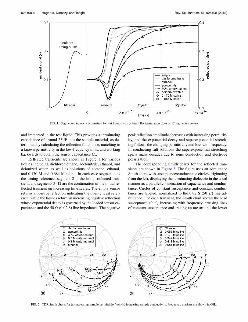
025108-4 Hager III, Domszy, and Tofighi Rev. Sci. Instrum. 83, 025108 (2012)

FIG. 1. Segmented transient acquisition for test liquids with 3.5-mm flat termination (four of 12 segments shown).

and immersed in the test liquid. This provides a terminatingcapacitance of around 25 fF into the sample material, as de-termined by calculating the reflection function ρ, matching toa known permittivity in the low-frequency limit, and workingbackwards to obtain the sensor capacitance Co.

Reflected transients are shown in Figure 1 for variousliquids including dichloromethane, acetonitrile, ethanol, anddeionized water, as well as solutions of acetone, ethanol,and 0.170 M and 0.684 M saline. In each case segment 1 isthe timing reference, segment 2 is the initial reflected tran-sient, and segments 3–12 are the continuation of the initial re-flected transient on increasing time scales. The empty sensorreturns a positive reflection indicating the open-circuit refer-ence, while the liquids return an increasing negative reflectionwhose exponential decay is governed by the loaded sensor ca-pacitance and the 50 � (0.02 S) line impedance. The negative

peak reflection amplitude decreases with increasing permittiv-ity, and the exponential decay and superexponential stretch-ing follows the changing permittivity and loss with frequency.In conducting salt solutions the superexponential stretchingspans many decades due to ionic conduction and electrodepolarization.

The corresponding Smith charts for the reflected tran-sients are shown in Figure 2. The figure uses an admittanceSmith chart, with susceptance/conductance circles originatingfrom the left, displaying the terminating dielectric in the usualmanner as a parallel combination of capacitance and conduc-tance. Circles of constant susceptance and constant conduc-tance are labeled, normalized to the 0.02 S (50 �) line ad-mittance. For each transient, the Smith chart shows the loadsusceptance ε′ωCo increasing with frequency, crossing linesof constant susceptance and tracing an arc around the lower

FIG. 2. TDR Smith charts for (a) increasing sample permittivity/loss (b) increasing sample conductivity. Frequency markers are shown in GHz.

025108-5 Hager III, Domszy, and Tofighi Rev. Sci. Instrum. 83, 025108 (2012)

FIG. 3. TDR Smith charts compared with (a) VNA measurement and (b) HFSS simulation. Frequency markers are shown in GHz.

perimeter of the chart. Select frequency points are labeled onthe diagram, starting at 1 GHz on the right and continuing to14 GHz on the left.

Figure 2 illustrates the Smith chart behavior for typi-cal variations in material properties. For an increasing realpermittivity the measured susceptance ε′ωCo increases morerapidly with frequency, showing a higher value at a given fre-quency and tracing a longer path around the lower perimeterof the diagram. This is clearly seen in Figure 2(a) for twolow-loss liquids, comparing high-permittivity acetonitrile (ε′

= 37.5) with low-permittivity dichloromethane (ε′ = 8.8).For an increasing loss, the conductance ε′′ ωCo also increaseswith frequency, tracing a path which spirals inward on thediagram crossing both circles of constant conductance andconstant susceptance. This is also seen in Figure 2(a), compar-ing liquids with increasing relaxation times τ such as acetoni-trile (τ = 2-3 ps), 30% water/acetone solution (τ = 10.1 ps)(Ref. 7) and 0.7 M and 0.4 M water/ethanol solution (τ= 45–85 ps),8 and pure ethanol (τ = 152 ps).8 For the ethanol,a peak representing the loss characteristics and sensor ca-pacitance is seen directly in the diagram around the relax-ation frequency of 1/2πτ . For an increasing ionic conduc-tivity, where the conductance remains constant over a widefrequency range,2 the trace follows a constant conductancecircle for each conductivity through the interior of the dia-gram. This is seen in Figure 2(b) for a series of water/saltsolutions with increasing salt concentration and ionic conduc-tivity. In addition, the very low frequency decrease in conduc-tivity with electrode polarization is seen in the slight “hook”appearing below 100 MHz.

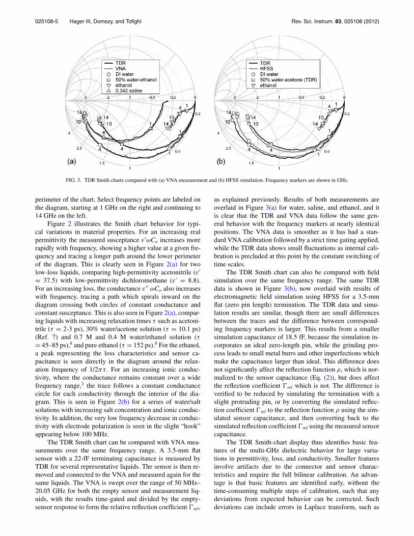
The TDR Smith chart can be compared with VNA mea-surements over the same frequency range. A 3.5-mm flatsensor with a 22-fF terminating capacitance is measured byTDR for several representative liquids. The sensor is then re-moved and connected to the VNA and measured again for thesame liquids. The VNA is swept over the range of 50 MHz–20.05 GHz for both the empty sensor and measurement liq-uids, with the results time-gated and divided by the empty-sensor response to form the relative reflection coefficient �rel,

as explained previously. Results of both measurements areoverlaid in Figure 3(a) for water, saline, and ethanol, and itis clear that the TDR and VNA data follow the same gen-eral behavior with the frequency markers at nearly identicalpositions. The VNA data is smoother as it has had a stan-dard VNA calibration followed by a strict time gating applied,while the TDR data shows small fluctuations as internal cali-bration is precluded at this point by the constant switching oftime scales.

The TDR Smith chart can also be compared with fieldsimulation over the same frequency range. The same TDRdata is shown in Figure 3(b), now overlaid with results ofelectromagnetic field simulation using HFSS for a 3.5-mmflat (zero pin length) termination. The TDR data and simu-lation results are similar, though there are small differencesbetween the traces and the difference between correspond-ing frequency markers is larger. This results from a smallersimulation capacitance of 18.5 fF, because the simulation in-corporates an ideal zero-length pin, while the grinding pro-cess leads to small metal burrs and other imperfections whichmake the capacitance larger than ideal. This difference doesnot significantly affect the reflection function ρ, which is nor-malized to the sensor capacitance (Eq. (2)), but does affectthe reflection coefficient �rel which is not. The difference isverified to be reduced by simulating the termination with aslight protruding pin, or by converting the simulated reflec-tion coefficient �rel to the reflection function ρ using the sim-ulated sensor capacitance, and then converting back to thesimulated reflection coefficient �rel using the measured sensorcapacitance.

The TDR Smith-chart display thus identifies basic fea-tures of the multi-GHz dielectric behavior for large varia-tions in permittivity, loss, and conductivity. Smaller featuresinvolve artifacts due to the connector and sensor charac-teristics and require the full bilinear calibration. An advan-tage is that basic features are identified early, without thetime-consuming multiple steps of calibration, such that anydeviations from expected behavior can be corrected. Suchdeviations can include errors in Laplace transform, such as

025108-6 Hager III, Domszy, and Tofighi Rev. Sci. Instrum. 83, 025108 (2012)

FIG. 4. TDR sensors for (a) 3.5-mm pin termination and (b) 9-mm flat ter-mination.

improper integration cursors and baseline settings, impropertruncation and tail fit settings, and excessive computation andnoise. They can also include errors in acquisition, such as tim-ing drift, segment mismatchs, connector artifacts, mechanicalsensor damage, and sensor design to be discussed next.

B. 3.5-mm sensor: Pin termination

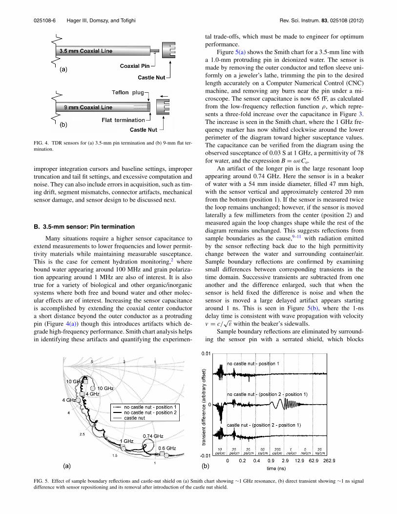
Many situations require a higher sensor capacitance toextend measurements to lower frequencies and lower permit-tivity materials while maintaining measurable susceptance.This is the case for cement hydration monitoring,2 wherebound water appearing around 100 MHz and grain polariza-tion appearing around 1 MHz are also of interest. It is alsotrue for a variety of biological and other organic/inorganicsystems where both free and bound water and other molec-ular effects are of interest. Increasing the sensor capacitanceis accomplished by extending the coaxial center conductora short distance beyond the outer conductor as a protrudingpin (Figure 4(a)) though this introduces artifacts which de-grade high-frequency performance. Smith chart analysis helpsin identifying these artifacts and quantifying the experimen-

tal trade-offs, which must be made to engineer for optimumperformance.

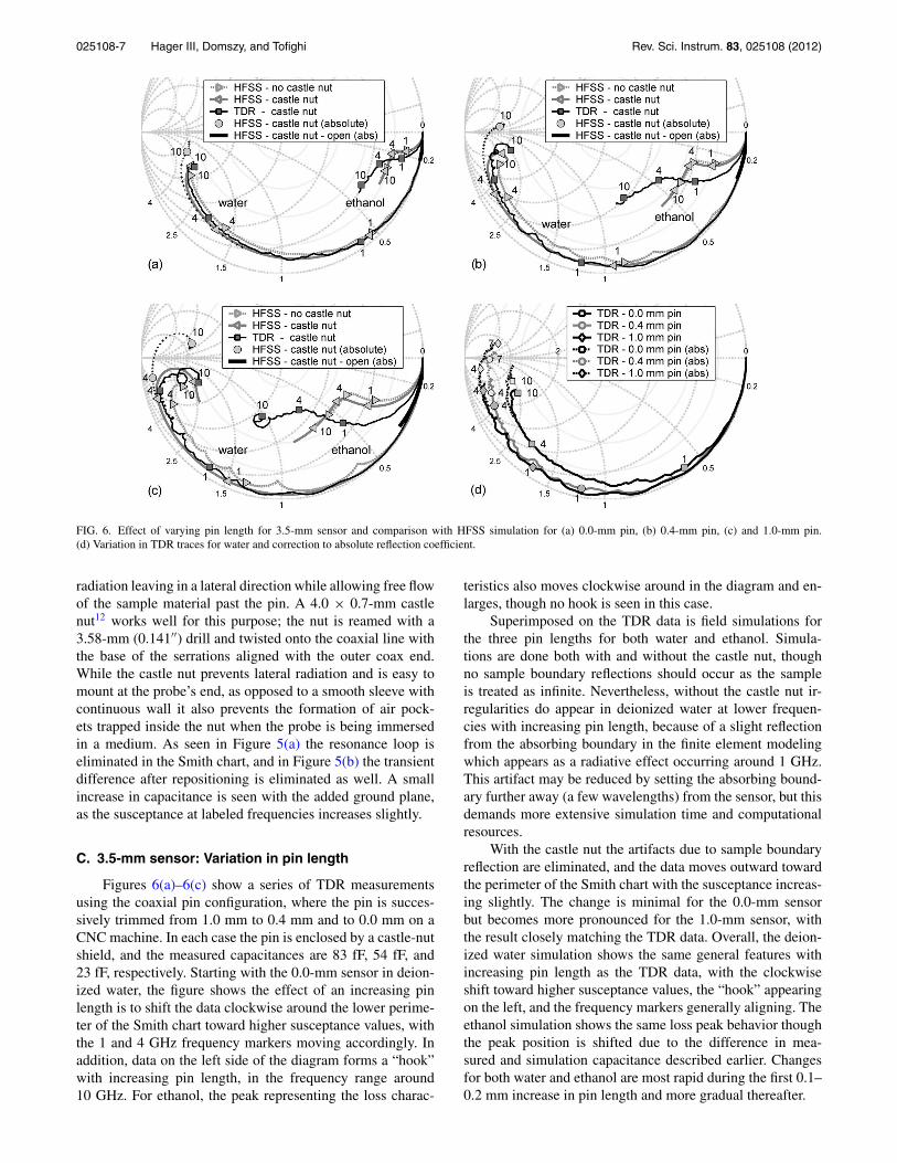
Figure 5(a) shows the Smith chart for a 3.5-mm line witha 1.0-mm protruding pin in deionized water. The sensor ismade by removing the outer conductor and teflon sleeve uni-formly on a jeweler’s lathe, trimming the pin to the desiredlength accurately on a Computer Numerical Control (CNC)machine, and removing any burrs near the pin under a mi-croscope. The sensor capacitance is now 65 fF, as calculatedfrom the low-frequency reflection function ρ, which repre-sents a three-fold increase over the capacitance in Figure 3.The increase is seen in the Smith chart, where the 1 GHz fre-quency marker has now shifted clockwise around the lowerperimeter of the diagram toward higher susceptance values.The capacitance can be verified from the diagram using theobserved susceptance of 0.03 S at 1 GHz, a permittivity of 78for water, and the expression B = ωεCo.

An artifact of the longer pin is the large resonant loopappearing around 0.74 GHz. Here the sensor is in a beakerof water with a 54 mm inside diameter, filled 47 mm high,with the sensor vertical and approximately centered 20 mmfrom the bottom (position 1). If the sensor is measured twicethe loop remains unchanged; however, if the sensor is movedlaterally a few millimeters from the center (position 2) andmeasured again the loop changes shape while the rest of thediagram remains unchanged. This suggests reflections fromsample boundaries as the cause,9–11 with radiation emittedby the sensor reflecting back due to the high permittivitychange between the water and surrounding container/air.Sample boundary reflections are confirmed by examiningsmall differences between corresponding transients in thetime domain. Successive transients are subtracted from oneanother and the difference enlarged, such that when thesensor is held fixed the difference is noise and when thesensor is moved a large delayed artifact appears startingaround 1 ns. This is seen in Figure 5(b), where the 1-nsdelay time is consistent with wave propagation with velocityv = c/

√ε within the beaker’s sidewalls.

Sample boundary reflections are eliminated by surround-ing the sensor pin with a serrated shield, which blocks

FIG. 5. Effect of sample boundary reflections and castle-nut shield on (a) Smith chart showing ∼1 GHz resonance, (b) direct transient showing ∼1 ns signaldifference with sensor repositioning and its removal after introduction of the castle nut shield.

025108-7 Hager III, Domszy, and Tofighi Rev. Sci. Instrum. 83, 025108 (2012)

FIG. 6. Effect of varying pin length for 3.5-mm sensor and comparison with HFSS simulation for (a) 0.0-mm pin, (b) 0.4-mm pin, (c) and 1.0-mm pin.(d) Variation in TDR traces for water and correction to absolute reflection coefficient.

radiation leaving in a lateral direction while allowing free flowof the sample material past the pin. A 4.0 × 0.7-mm castlenut12 works well for this purpose; the nut is reamed with a3.58-mm (0.141′′) drill and twisted onto the coaxial line withthe base of the serrations aligned with the outer coax end.While the castle nut prevents lateral radiation and is easy tomount at the probe’s end, as opposed to a smooth sleeve withcontinuous wall it also prevents the formation of air pock-ets trapped inside the nut when the probe is being immersedin a medium. As seen in Figure 5(a) the resonance loop iseliminated in the Smith chart, and in Figure 5(b) the transientdifference after repositioning is eliminated as well. A smallincrease in capacitance is seen with the added ground plane,as the susceptance at labeled frequencies increases slightly.

C. 3.5-mm sensor: Variation in pin length

Figures 6(a)–6(c) show a series of TDR measurementsusing the coaxial pin configuration, where the pin is succes-sively trimmed from 1.0 mm to 0.4 mm and to 0.0 mm on aCNC machine. In each case the pin is enclosed by a castle-nutshield, and the measured capacitances are 83 fF, 54 fF, and23 fF, respectively. Starting with the 0.0-mm sensor in deion-ized water, the figure shows the effect of an increasing pinlength is to shift the data clockwise around the lower perime-ter of the Smith chart toward higher susceptance values, withthe 1 and 4 GHz frequency markers moving accordingly. Inaddition, data on the left side of the diagram forms a “hook”with increasing pin length, in the frequency range around10 GHz. For ethanol, the peak representing the loss charac-

teristics also moves clockwise around in the diagram and en-larges, though no hook is seen in this case.

Superimposed on the TDR data is field simulations forthe three pin lengths for both water and ethanol. Simula-tions are done both with and without the castle nut, thoughno sample boundary reflections should occur as the sampleis treated as infinite. Nevertheless, without the castle nut ir-regularities do appear in deionized water at lower frequen-cies with increasing pin length, because of a slight reflectionfrom the absorbing boundary in the finite element modelingwhich appears as a radiative effect occurring around 1 GHz.This artifact may be reduced by setting the absorbing bound-ary further away (a few wavelengths) from the sensor, but thisdemands more extensive simulation time and computationalresources.

With the castle nut the artifacts due to sample boundaryreflection are eliminated, and the data moves outward towardthe perimeter of the Smith chart with the susceptance increas-ing slightly. The change is minimal for the 0.0-mm sensorbut becomes more pronounced for the 1.0-mm sensor, withthe result closely matching the TDR data. Overall, the deion-ized water simulation shows the same general features withincreasing pin length as the TDR data, with the clockwiseshift toward higher susceptance values, the “hook” appearingon the left, and the frequency markers generally aligning. Theethanol simulation shows the same loss peak behavior thoughthe peak position is shifted due to the difference in mea-sured and simulation capacitance described earlier. Changesfor both water and ethanol are most rapid during the first 0.1–0.2 mm increase in pin length and more gradual thereafter.

025108-8 Hager III, Domszy, and Tofighi Rev. Sci. Instrum. 83, 025108 (2012)

The “hook” appearing on the left in water is an artifact ofthe relative reflection coefficient �rel analysis, since the reflec-tion coefficient is calculated relative to the empty-sensor re-flection rather than the actual input stimulus. The input stim-ulus is not used in the TDR measurement since its timing isarbitrary relative to the sensor reflection, and since acquisitionof the input stimulus over the relevant time scales would nec-essarily include the reflected pulse. The hook is removed bymultiplying by the absolute reflection coefficient of the emptysensor, since the absolute reflection coefficient can be writtenas �x = �rel �r from Eq. (7). The absolute reflection coeffi-cient of the empty sensor can be obtained either by simulationor by solving Eq. (1) for �r with ε = 1,

�r = vr,r

vi= Gc − iωCo

Gc + iωCo. (8)

Figures 6(a)–6(c) also show the absolute reflection coefficientfor each pin length in water obtained by simulation. For the0.0-mm pin the deviation between relative and absolute reflec-tion coefficients is small, while for the 0.4- and 1.0-mm pinsit is much larger. The deviation becomes more pronouncedat higher frequencies starting around 4 GHz and above(depending on pin length), which coincides with the fre-quency range of the absolute reflection coefficient crossinginto the inductive region, showing resonance behavior withthe sensor acting as an antenna. For the TDR data, the ab-solute reflection coefficient is estimated by multiplying therelative reflection coefficient by the simulated reflection coef-ficient of the empty sensor or by Eq. (8), where the simulationis slightly more accurate as it incorporates radiation effects ofthe empty sensor at high frequencies.

The absolute reflection coefficients for the three pinlengths are shown in Figure 6(d), and it is clear for the0.4-mm and 1.0-mm pins that the data crosses into the induc-tive region in water in the 4–10 GHz range. For the 1.0-mmpin in water, the exact resonance frequency of the absolute re-flection coefficient (where its angle becomes −180◦) obtainedby HFSS is 5.2 GHz with the castle nut (Figure 6(c), where theabsolute reflection coefficient crosses the horizontal axis) and7.2 GHz without it (not shown), which compares well with thequarter wave resonance of an ideal 1.0-mm long monopoleantenna in water medium at about 8 GHz. For TDR Smith-chart display of the relative reflection coefficient, such a reso-nance is manifested by the presence of the mentioned hook inthe corresponding trace. In addition, if Eq. (1) is rewritten interms of the absolute reflection coefficient, similar to Eq. (6),the resulting real and imaginary components show rapid vari-ation around the resonance frequency (where angle of �abs

= −180◦) as expected for quarter-wave behavior.1

D. 3.5-mm sensor: Effect on bilinear calibration

Artifacts revealed by Smith chart analysis can be tracedthrough the bilinear calibration process to the final permit-tivity. For example, sample boundary reflections appearing inFigure 5 and pin artifacts appearing in Figure 6 enter into thereflection function ρ(ω) through Eq. (6). Two liquid measure-ments are required for each calibration, so artifacts appearingin ρcal,1(ω) and ρcal,2(ω) appear in the solution of simultane-

ous equations for A(ω) and B(ω) in Eq. (5). Artifacts appear-ing in A(ω) and B(ω) enter the unknown calibration throughEq. (4), and are compounded by similar artifacts appearingin the reflection function of the unknown ρunk(ω) in the finalresult.

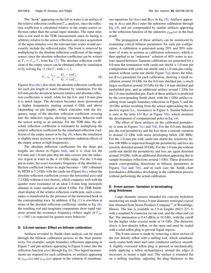
The propagation of these artifacts can be monitored byexamining critical bilinear parameters for each pin configu-ration. A calibration is generated using 20% and 50% solu-tions of water in acetone as calibration references, which isthen applied to an “unknown” solution of 40% water in ace-tone spaced between. Separate calibrations are generated for a0.0-mm flat termination with castle-nut shield, a 1.0-mm pinconfiguration with castle-nut shield, and a 1.0-mm pin config-uration without castle-nut shield. Figure 7(a) shows the bilin-ear B′(ω) parameter for each calibration, showing a small os-cillation around 10 GHz for the 0.0 mm shielded pin, a muchlarger oscillation around 10 GHz for the 1.0-mm shielded andunshielded pins, and an additional artifact around 1 GHz forthe 1.0-mm unshielded pin. Each of these artifacts is predictedby the corresponding Smith chart, with the 1 GHz artifact re-sulting from sample boundary reflections in Figure 5, and the10 GHz artifact resulting from the sensor approaching the in-ductive region (i.e., resonance) in Figure 6. Similar behavioris seen in the term 1/|1-Bρ| in Figure 7(b), which monitorsthe development of computational poles in Eq. (4).

The effect of these artifacts on the calibrated permittiv-ity is seen in Figures 7(c) and 7(d). For the 0.0-mm shieldedpin, the real permittivity and the loss show a smooth variationto around 12 GHz with noise developing below 100 MHz.For the 1.0-mm pin with castle-nut shield the sensitivity be-low 100 MHz is improved though the permittivity and loss areseverely distorted around 10 GHz. For the 1.0-mm pin withoutcastle-nut shield the permittivity and loss are again distortedaround 10 GHz, with an additional distortion appearing due tosample boundary reflections around 1 GHz. These distortionsmatch corresponding distortions in bilinear parameters inFigures 7(a) and 7(b), and in each case the Smith chartforeshadows difficulties developing in the calibration processwithout performing the actual calibration.

E. 9-mm sensor: Variation in terminatingplug thickness

Large diameter sensors intended for concrete hydrationmonitoring are made from a 9-mm diameter semirigid coaxialline obtained from Storm Products Company13 of Woodridge,Illinois. The line is available in 1.5-m lengths (#421-227-3)with a standard N connector on one end, and the other end cutflat. The attenuation is 0.43 dB/m at 10 GHz, with the cutofffor the higher order coaxial mode at 14 GHz. The dielectricsleeve is low-density teflon, so the open end must be sealedwith a solid teflon plug to prevent liquid ingress.

The 9-mm sensor is made by removing a short section ofthe low density teflon with a milling tool, which simultane-ously reams both inner and outer conductor surfaces smooth.A slightly oversized teflon plug is pressed in mechanically,while applying a teflon etchant/epoxy around the edges ifnecessary to insure a tight seal. The surface is trimmed flaton a milling machine, adjusting the plug thickness to the

025108-9 Hager III, Domszy, and Tofighi Rev. Sci. Instrum. 83, 025108 (2012)

FIG. 7. Effect of pin length and castle-nut shield on bilinear parameters (a) B′, (b) 1 / |1-Bρ |, and calibrated permittivity (c) ε′ and d) ε′′ (3.5-mm sensor in 40%water/acetone solution).

desired length. The line is connected to the TDR input with anN-to-SMA adapter, mechanically clamping in place to insureno strain on the TDR input. To insure a consistent measure-ment plane, the sensor is leak-tested in acetone by monitor-ing the signal to make sure it remains constant over a periodof time and returns to its original position when solvent isremoved. The resulting sensor provides ∼60-fF load capaci-tance as shown in Figure 4(b).

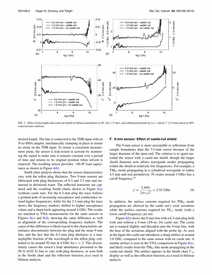
Smith chart analysis shows that the sensor characteristicsvary with the teflon plug thickness. Two 9-mm sensors arefabricated with plug thicknesses of 6.3 and 2.5 mm and im-mersed in deionized water. The reflected transients are cap-tured and the resulting Smith charts shown in Figure 8(a)(without castle nut). For the 6.3-mm plug the trace followsa gradual path of increasing susceptance and conductance to-ward higher frequencies, while for the 2.5-mm plug the traceshows the frequency markers shifted to higher susceptancevalues and a sharp hook appearing around 4 GHz. The resultsare matched to VNA measurements for the same sensors inFigures 8(c) and 8(d), showing the same difference as wellas alignment of the corresponding frequency markers. Thecause of this difference is likely traced to the characteristic ad-mittance discontinuity between the plug and the main 9-mmline, and the fact that the 6.3-mm plug thickness is a non-negligible fraction of the wavelength in the teflon plug, esti-mated to be around 50 mm at 4 GHz for ε = 2. This discon-tinuity causes the sensor’s load admittance presented to the50 � (0.02 S) line to vary with plug thickness, as seen bothin the Smith chart and the reflection function ρ(ω) used inbilinear analysis.

F. 9-mm sensor: Effect of castle-nut shield

The 9-mm sensor is more susceptible to reflections fromsample boundaries than the 3.5-mm sensor because of thelarger diameter of the open end. The solution is to again sur-round the sensor with a castle-nut shield, though the largershield diameter now allows waveguide modes propagatingwithin the shield at relatively low frequencies. For example, aTM01 mode propagating in a cylindrical waveguide or radius4.5 mm and real permittivity 76 (water around 3 GHz) has acutoff frequency:14

f = 2.405c

2πr√

ε′ = 2.92 GHz. (9)

In addition, the surface currents required for TM01 modepropagation are allowed by the castle nut’s axial serrationswhile the surface currents required for TE11 mode (with alower cutoff frequency) are not.

Figure 8(b) shows the 9-mm line with a 6.3-mm plug bothwith and without a 9-mm (3/8-in.-24) castle nut. The castlenut is reamed slightly and threaded onto the 9-mm line, withthe base of the serrations aligned with the probe tip. As seenin the figure the castle nut introduces a sharp artifact at around3.8 GHz, compared to the same sensor with no castle nut. Asimilar artifact is seen in the VNA comparison in Figure 8(e),and likely results from the TM01-like mode propagating in thecastle-nut shield. The artifact appears in the Smith chart �rel

display as well as the reflection function ρ(ω) used in bilinearanalysis.

025108-10 Hager III, Domszy, and Tofighi Rev. Sci. Instrum. 83, 025108 (2012)

FIG. 8. Effect of terminating plug thickness and castle-nut shield on 9-mm flat termination in water. (a) 6.3 vs. 2.5-mm plug without castle-nut shield,(b) 6.3-mm plug with/without castle-nut shield, (c) 2.5-mm plug without castle-nut shield compared with VNA, (d) 6.3-mm plug without castle-nut shieldcompared with VNA, and (e) 6.3-mm plug with castle-nut shield compared with VNA.

V. DISCUSSION

We have demonstrated a TDR Smith-chart display tobe a valuable diagnostic tool for a variety of situations inTDR dielectric spectroscopy. A relative reflection coefficientis formed by dividing the Laplace transform of the reflectedsample transient by the Laplace transform of the empty-sensor transient and displaying it in the complex plane, withthe approximate sensor admittance read from the suscep-tance and conductance circles. The Smith-chart display pro-vides an initial estimate of the dielectric behavior in themulti-GHz range, as well as a means of identifying arti-facts in acquisition or Laplace transform, in a way whichdoes not require multiple steps of calibration and is onlyone step removed from the direct transient. Since the rela-tive reflection coefficient is derived from the bilinear reflec-tion function ρ(ω), artifacts occurring in the relative reflec-tion coefficient foreshadow artifacts occurring in the bilinearcalibration.

Results were presented for a simple 3.5-mm flat termi-nation, showing variations in Smith chart behavior for typi-cal variations in sample permittivity, loss, and, conductivity.Results were matched to VNA measurement over an identi-cal frequency range, as well as to finite-element field simu-lation. Results were also presented for a 3.5-mm sensor withincreased terminating pin lengths, typically employed at lowfrequencies and low permittivity media to increase sensorcapacitance. Measurements were made as a function of pinlength and compared with simulation, for pin lengths between0.0 and 1.0 mm both with and without a surrounding shield.For an unshielded pin, the Smith chart analysis detects reflec-tions from sample boundaries and provides a means of mea-

suring the effectiveness of shielding used to eliminate thesereflections. For a shielded pin, the Smith chart characterizesthe effect of pin length on the susceptance variation and theadmittance’s approach toward resonance at high frequenciesand high permittivity samples. A “hook” appearing at highfrequencies at longer pin lengths was shown to be an artifactof the relative reflection coefficient, and a method for cor-recting it to an absolute reflection coefficient was explored.The effect of artifacts appearing in the Smith chart on theactual calibration was shown by tracking them through thecalibration process to the final result. Finally, results werepresented for a 9-mm flat termination used for concrete hy-dration monitoring, showing effects of the sensor’s terminat-ing admittance transformation within a terminating plug andthe onset of waveguide modes in a surrounding shield, withresults compared to VNA measurement.

It is well known that the admittance of an open-end sen-sor can deviate significantly from the simple air-terminatedcapacitance C0 at multi-GHz frequencies.3, 15 The sensor canact as a resonating antenna, with the terminating admit-tance moving from capacitive to inductive region as seen inFigure 6. This resonance can produce artifacts which appearin the calibrated sample permittivity in Figure 7, which isimpacted both by the choice of pin length and surroundingshield. Our preliminary studies suggest that an increase inpin length and the presence of a castle-nut shield lead to theresonance frequency moving to lower frequencies, and futurework will include a quantification of this resonance limit forboth the 3.5- and 9-mm sensors. Incorporation of the radiationmodel3, 15 in characterizing the unknown permittivity will bealso studied.

025108-11 Hager III, Domszy, and Tofighi Rev. Sci. Instrum. 83, 025108 (2012)

ACKNOWLEDGMENTS

This work was supported in part by the National ScienceFoundation (NSF) under Grant No. 0700699.

1R. H. Cole, J. G. Berberian, S. Mashimo, G. Chryssikos, A. Burns, andE. Tombari, J. Appl. Phys. 66, 793 (1989).

2N. E. Hager III and R. C. Domszy, J. Appl. Phys. 96, 5117 (2004).3D. Misra, M. Chabbra, B. R. Epstein, M. Mirotznik, and K. R. Foster, IEEETrans. Microwave Theory Tech. 38(1), 8 (1990).

4N. E. Hager III, Rev. Sci. Instrum. 65, 887 (1994).5F. 1. Mopsik, Rev. Sci. Instrum. 55, 79 (1985).6M. R. Tofighi and A. S. Daryoush, IEEE Trans. Instrum. Meas. 58(7), 2316,(2009).

7A. C. Kumbharkhane, S. N. Helambe, M. P. Lokhande, S. Doraiswamy,and S. H, Mehrotra, Pramana, J. Phys. 46(2), 91 (1996).

8S. Mashimo, T. Umehara, and H. Redlin, J. Chem. Phys. 95(9), 6257(1991).

9S. Evans and A. bin Azeman, Phys. Med. Biol. 43, 2817 (1998).10T. P. Marsland and S. Evans, IEE Proceedings H 134(4), 341 (1987).11D. M. Hagl, D. Popovic, S. C. Hagness, J. H. Booske, and M. Okoniewski,

IEEE Trans. Microwave Theory Tech. 51(4), 1194 (2003).12Metric & Multistandard Components Corp., Hawthorne, NY, Part #935.13Storm Products Company, Woodridge, Illinois, see

www.stormproducts.com.14S. Y. Liao, Microwave Devices and Circuits (Prentice-Hall, Englewood

Cliffs, NJ, 1980), p. 119.15A. Nyshadham, C. L. Sibbald, and S. S. Stuchly, IEEE Trans. Microwave

Theory Tech. 40(2), 305 (1992).