192
NIST Special Publication 1017-1 Smokeview (Version 6) - A Tool for Visualizing Fire Dynamics Simulation Data Volume I: User’s Guide Glenn P. Forney

NIST Special Publication 1017-1
Smokeview (Version 6) - A Tool for
Visualizing Fire Dynamics Simulation Data
Volume I: User’s Guide
Glenn P. Forney


NIST Special Publication 1017-1
Smokeview (Version 6) - A Tool for
Visualizing Fire Dynamics Simulation Data
Volume I: User’s Guide
Glenn P. Forney
Fire Research DivisionEnginnering Laboratory
June 20, 2012
Smokeview Version 6
SV NRepository Revision : 11111
UN
ITEDSTATES OF AMER
ICA
DEPA
RTMENT OF COMMERCE
U.S. Department of Commerce
John E. Bryson, Secretary
National Institute of Standards and Technology
Patrick D. Gallagher, Under Secretary of Commerce for Standards and Technology and Director

Certain commercial entities, equipment, or materials may be identified in this
document in order to describe an experimental procedure or concept adequately. Such
identification is not intended to imply recommendation or endorsement by the
National Institute of Standards and Technology, nor is it intended to imply that the
entities, materials, or equipment are necessarily the best available for the purpose.
National Institute of Standards and Technology Special Publication 1017-1Natl. Inst. Stand. Technol. Spec. Publ. 1017-1, 184 pages (July 2008)
CODEN: NSPUE2
U.S. GOVERNMENT PRINTING OFFICEWASHINGTON: 2007
For sale by the Superintendent of Documents, U.S. Government Printing OfficeInternet: bookstore.gpo.gov – Phone: (202) 512-1800 – Fax: (202) 512-2250
Mail: Stop SSOP, Washington, DC 20402-0001

Preface
Smokeview is a software tool designed to visualize numerical calculations generated by fire models such as
the Fire Dynamics Simulator (FDS), a computational fluid dynamics (CFD) model of fire-driven fluid flow
or CFAST, a zone fire model. Smokeview visualizes smoke and other attributes of the fire using traditional
scientific methods such as displaying tracer particle flow, 2D or 3D shaded contours of gas flow data such
as temperature and flow vectors showing flow direction and magnitude. Smokeview also visualizes fire
attributes realistically so that one can experience the fire. This is done by displaying a series of partially
transparent planes where the transparencies in each plane (at each grid node) are determined from soot
densities computed by FDS. Smokeview also visualizes static data at particular times again using 2D or 3D
contours of data such as temperature and flow vectors showing flow direction and magnitude.
Smokeview and associated documentation for Windows, Linux and Mac/OSX may be downloaded from
the web site http://fire.nist.gov/fds at no cost.
i

ii

About the Author
Glenn Forney is a computer scientist at the Engineering Laboratory of NIST. He received a bachelor of
science degree in mathematics from Salisbury State College in 1978 and a master of science and a
doctorate in mathematics at Clemson University in 1980 and 1984. He joined the NIST staff in 1986
(then the National Bureau of Standards) and has since worked on developing tools that provide a
better understanding of fire phenomena, most notably Smokeview, a software tool for visualizing Fire
Dynamics Simulation data.
iii

iv

Disclaimer
The US Department of Commerce makes no warranty, expressed or implied, to users of Smokeview, and
accepts no responsibility for its use. Users of Smokeview assume sole responsibility under Federal law for
determining the appropriateness of its use in any particular application; for any conclusions drawn from the
results of its use; and for any actions taken or not taken as a result of analysis performed using this tools.
Smokeview and the companion program FDS is intended for use only by those competent in the fields
of fluid dynamics, thermodynamics, combustion, and heat transfer, and is intended only to supplement the
informed judgment of the qualified user. These software packages may or may not have predictive capability
when applied to a specific set of factual circumstances. Lack of accurate predictions could lead to erroneous
conclusions with regard to fire safety. All results should be evaluated by an informed user.
Throughout this document, the mention of computer hardware or commercial software does not con-
stitute endorsement by NIST, nor does it indicate that the products are necessarily those best suited for the
intended purpose.
v

vi

Acknowledgements
A number of people have made significant contributions to the development of Smokeview. In trying to
acknowledge those that have contributed, we are inevitably going to miss a few people. Let us know and we
will include those missed in the next version of this guide.
The original version of Smokeview was inspired by Frames, a visualization program written by James
Sims for the Silicon Graphics workstation. This software was based on visualization software written by
Stuart Cramer for an Evans and Sutherland computer. Frames used tracer particles to visualize smoke flow
computed by a pre-cursor to FDS. Judy Devaney made the multi-screen eight foot Rave facility available
allowing a stereo version of Smokeview to be built that can display scenes in 3D. Both Steve Satterfield
and Tere Griffin on many occasions helped me demonstrate Smokeview cases on the Rave inspiring many
people to the possibility of using Smokeview as a virtual reality-like fire fighter training facility.
Many conversations with Nelson Bryner, Dave Evans, Anthony Hamins and Doug Walton were most
helpful in determining how Smokeview could be adapted for use in fire fighter training applications.
Smokeview would not be possible without the use of a number of software libraries developed by others.
Mark Kilgard while at Silicon Graphics developed GLUT, the basic tool kit for interfacing OpenGL with the
underlying operating system on multiple computer platforms. Paul Rademacher while a graduate student at
the University of North Carolina developed GLUI, the software library for implementing the user friendly
dialog boxes.
Significant contributions have been made by those that have used Smokeview to visualize complex
cases; cases that are used to perform both applied and basic research. The resulting feedback has improved
Smokeview as a result of their interaction with me, pushing the envelope and not accepting the status quo.
For applied research, Daniel Madrzykowski, Doug Walton and Robert Vettori of NIST have used
Smokeview to analyze fire incidents. Steve Kerber has used Smokeview to visualize flows resulting from
positive pressure ventilation (PPV) fans. David Stroup has used Smokeview to analyze cases for use in fire
fighter training scenarios. Conversations with Doug Walton have been particularly helpful in identifying
needed features and clarifying how best to make their implementation user friendly. David Evans, William
(Ruddy) Mell and Ronald Rehm used Smokeview to visualize urban-wildland interface fires. For basic
research, Greg Linteris has used Smokeview to visualize fire simulations involving the cone calorimeter.
Anthony Hamins has used Smokeview to visualize the structure of CH4/air flames undergoing the transi-
tion from normal to microgravity conditions and fire suppression in a compartment. Jiann Yang has used
Smokeview to visualize smoke or particle number density and saturation ratio of condensable vapor.
This user’s guide has improved through the many constructive comments of the reviewers Anthony
Hamins, Doug Walton, Ronald Rehm, and David Sheppard. Chuck Bouldin helped port Smokeview to the
Macintosh.
Many people have sent in multiple comments and feedback by email, in particular Adrian Brown, Scot
Deal, Charlie Fleischmann, Jason Floyd, Simo Hostikka, Bryan Klein, Davy Leroy, Dave McGill, Brian
McLaughlin, Derek Nolan, Steven Olenick, Stephen Priddy, Boris Stock, Jason Sutula, Javier Trelles, and
Christopher Wood.
Feedback is encouraged and may be sent to [email protected] .
vii

viii

Contents
Preface i
About the Author iii
Disclaimer v
I Using Smokeview 1
1 Introduction 31.1 Overview . . . . . . . . . . . . . . . . . . . . . . . . . . . . . . . . . . . . . . . . . . . . 3
1.2 Features . . . . . . . . . . . . . . . . . . . . . . . . . . . . . . . . . . . . . . . . . . . . . 4
1.2.1 Visualizing Data . . . . . . . . . . . . . . . . . . . . . . . . . . . . . . . . . . . . 5
1.2.2 Exploring Data . . . . . . . . . . . . . . . . . . . . . . . . . . . . . . . . . . . . . 6
1.2.3 Exploring the Scene . . . . . . . . . . . . . . . . . . . . . . . . . . . . . . . . . . 7
1.2.4 Customizing the Scene . . . . . . . . . . . . . . . . . . . . . . . . . . . . . . . . . 7
1.2.5 Automating the Visualization . . . . . . . . . . . . . . . . . . . . . . . . . . . . . 8
1.3 Getting Started . . . . . . . . . . . . . . . . . . . . . . . . . . . . . . . . . . . . . . . . . 8
1.3.1 Obtaining Smokeview . . . . . . . . . . . . . . . . . . . . . . . . . . . . . . . . . 8
1.3.2 Running Smokeview . . . . . . . . . . . . . . . . . . . . . . . . . . . . . . . . . . 8
2 Manipulating the Scene 112.1 World View . . . . . . . . . . . . . . . . . . . . . . . . . . . . . . . . . . . . . . . . . . . 11
2.2 Eye View . . . . . . . . . . . . . . . . . . . . . . . . . . . . . . . . . . . . . . . . . . . . 14
3 Visualizing Smoke 173.1 Tracers and Streaklines . . . . . . . . . . . . . . . . . . . . . . . . . . . . . . . . . . . . . 17
3.2 Realistic . . . . . . . . . . . . . . . . . . . . . . . . . . . . . . . . . . . . . . . . . . . . . 17
4 Visualizing Data Quantitatively 214.1 2D Shaded Contours and Vector Slices - Slice Files . . . . . . . . . . . . . . . . . . . . . . 21
4.1.1 Axis aligned slices . . . . . . . . . . . . . . . . . . . . . . . . . . . . . . . . . . . 21
4.1.2 3D slices . . . . . . . . . . . . . . . . . . . . . . . . . . . . . . . . . . . . . . . . 25
4.1.3 Fractional effective dose (FED) slices . . . . . . . . . . . . . . . . . . . . . . . . . 25
4.2 2D Shaded Contours on Solid Surfaces - Boundary Files . . . . . . . . . . . . . . . . . . . 27
4.3 3D Contours - Isosurface Files . . . . . . . . . . . . . . . . . . . . . . . . . . . . . . . . . 28
4.3.1 Isosurfaces for fractional effective dose data . . . . . . . . . . . . . . . . . . . . . . 32
4.4 Device data - .csv files . . . . . . . . . . . . . . . . . . . . . . . . . . . . . . . . . . . . . 32
ix

4.5 Static Data - Plot3D Files . . . . . . . . . . . . . . . . . . . . . . . . . . . . . . . . . . . . 32
5 Visualizing Zone Fire Data 37
II Controlling and Customizing Smokeview 41
6 Setting Options 436.1 Setting Data Bounds . . . . . . . . . . . . . . . . . . . . . . . . . . . . . . . . . . . . . . 43
6.2 3D Smoke Options . . . . . . . . . . . . . . . . . . . . . . . . . . . . . . . . . . . . . . . 43
6.3 Plot3D Viewing Options . . . . . . . . . . . . . . . . . . . . . . . . . . . . . . . . . . . . 48
6.3.1 2D contours . . . . . . . . . . . . . . . . . . . . . . . . . . . . . . . . . . . . . . . 48
6.3.2 Iso-Contours . . . . . . . . . . . . . . . . . . . . . . . . . . . . . . . . . . . . . . 48
6.3.3 Flow vectors . . . . . . . . . . . . . . . . . . . . . . . . . . . . . . . . . . . . . . 48
6.4 Display Options . . . . . . . . . . . . . . . . . . . . . . . . . . . . . . . . . . . . . . . . . 48
6.4.1 General . . . . . . . . . . . . . . . . . . . . . . . . . . . . . . . . . . . . . . . . . 48
6.4.2 Stereo . . . . . . . . . . . . . . . . . . . . . . . . . . . . . . . . . . . . . . . . . . 48
6.5 Clipping Scenes . . . . . . . . . . . . . . . . . . . . . . . . . . . . . . . . . . . . . . . . . 50
7 Creating Custom Objects 557.1 Object File Format . . . . . . . . . . . . . . . . . . . . . . . . . . . . . . . . . . . . . . . 55
7.2 Elementary Geometric Objects . . . . . . . . . . . . . . . . . . . . . . . . . . . . . . . . . 56
7.3 Visual Transformations . . . . . . . . . . . . . . . . . . . . . . . . . . . . . . . . . . . . . 63
7.4 Arithmetic Transformations . . . . . . . . . . . . . . . . . . . . . . . . . . . . . . . . . . . 64
7.5 Logical and Conditional Operators . . . . . . . . . . . . . . . . . . . . . . . . . . . . . . . 66
8 Manipulating the Scene Automatically - The Touring Option 698.1 Tour Settings . . . . . . . . . . . . . . . . . . . . . . . . . . . . . . . . . . . . . . . . . . 69
8.2 Keyframe Settings . . . . . . . . . . . . . . . . . . . . . . . . . . . . . . . . . . . . . . . . 69
8.3 Advanced Settings . . . . . . . . . . . . . . . . . . . . . . . . . . . . . . . . . . . . . . . 70
8.4 Setting up a tour . . . . . . . . . . . . . . . . . . . . . . . . . . . . . . . . . . . . . . . . . 72
9 Running Smokeview Automatically - The Scripting Option 759.1 Overview . . . . . . . . . . . . . . . . . . . . . . . . . . . . . . . . . . . . . . . . . . . . 75
9.2 Creating a Script . . . . . . . . . . . . . . . . . . . . . . . . . . . . . . . . . . . . . . . . 75
9.2.1 Example 1 . . . . . . . . . . . . . . . . . . . . . . . . . . . . . . . . . . . . . . . 75
9.2.2 Example 2 . . . . . . . . . . . . . . . . . . . . . . . . . . . . . . . . . . . . . . . 79
9.3 Script Glossary . . . . . . . . . . . . . . . . . . . . . . . . . . . . . . . . . . . . . . . . . 81
9.3.1 Loading and Unloading Files . . . . . . . . . . . . . . . . . . . . . . . . . . . . . . 82
9.3.2 Controlling the Scene . . . . . . . . . . . . . . . . . . . . . . . . . . . . . . . . . . 85
9.3.3 Rendering Images . . . . . . . . . . . . . . . . . . . . . . . . . . . . . . . . . . . 86
III Miscellaneous Topics 87
10 Coloring Data 8910.1 Overview . . . . . . . . . . . . . . . . . . . . . . . . . . . . . . . . . . . . . . . . . . . . 89
10.2 Using the Colorbar Editor . . . . . . . . . . . . . . . . . . . . . . . . . . . . . . . . . . . . 89
x

11 Smokeview - Demonstrator Mode 93
12 Texture Maps 95
13 Using Smokeview to Debug FDS Input Files 9713.1 Examining Blockages . . . . . . . . . . . . . . . . . . . . . . . . . . . . . . . . . . . . . . 98
14 Making Movies 99
15 Annotating the Scene 10115.1 Overview . . . . . . . . . . . . . . . . . . . . . . . . . . . . . . . . . . . . . . . . . . . . 101
15.2 User Ticks Settings Dialog Box . . . . . . . . . . . . . . . . . . . . . . . . . . . . . . . . . 101
15.3 TICKS and LABELS keywords . . . . . . . . . . . . . . . . . . . . . . . . . . . . . . . . 101
16 Utilities 10516.1 Compression - Using Smokezip to reduce FDS file sizes . . . . . . . . . . . . . . . . . . . 105
16.2 Differencing - Using Smokediff to compare two FDS cases . . . . . . . . . . . . . . . . . . 107
16.3 Background - A utility to run multiple Windows programs simultaneously . . . . . . . . . . 108
17 Summary 111
References 114
IV Appendices 115
Appendices 117
A Command Line Options 117
B Menu Options 119B.1 Main . . . . . . . . . . . . . . . . . . . . . . . . . . . . . . . . . . . . . . . . . . . . . . . 119
B.2 Load/Unload . . . . . . . . . . . . . . . . . . . . . . . . . . . . . . . . . . . . . . . . . . 119
B.3 Show/Hide . . . . . . . . . . . . . . . . . . . . . . . . . . . . . . . . . . . . . . . . . . . 122
B.3.1 Geometry Options . . . . . . . . . . . . . . . . . . . . . . . . . . . . . . . . . . . 122
B.3.2 Labels . . . . . . . . . . . . . . . . . . . . . . . . . . . . . . . . . . . . . . . . . . 123
B.3.3 Data coloring . . . . . . . . . . . . . . . . . . . . . . . . . . . . . . . . . . . . . . 123
B.3.4 Viewpoints . . . . . . . . . . . . . . . . . . . . . . . . . . . . . . . . . . . . . . . 123
B.3.5 Flip . . . . . . . . . . . . . . . . . . . . . . . . . . . . . . . . . . . . . . . . . . . 125
B.3.6 Animated Surface . . . . . . . . . . . . . . . . . . . . . . . . . . . . . . . . . . . . 125
B.3.7 Particles . . . . . . . . . . . . . . . . . . . . . . . . . . . . . . . . . . . . . . . . . 125
B.3.8 Boundary . . . . . . . . . . . . . . . . . . . . . . . . . . . . . . . . . . . . . . . . 125
B.3.9 Animated Vector Slice . . . . . . . . . . . . . . . . . . . . . . . . . . . . . . . . . 125
B.3.10 Animated Slice . . . . . . . . . . . . . . . . . . . . . . . . . . . . . . . . . . . . . 125
B.3.11 Plot3D . . . . . . . . . . . . . . . . . . . . . . . . . . . . . . . . . . . . . . . . . 125
B.3.12 Textures . . . . . . . . . . . . . . . . . . . . . . . . . . . . . . . . . . . . . . . . . 126
B.4 Options . . . . . . . . . . . . . . . . . . . . . . . . . . . . . . . . . . . . . . . . . . . . . 126
B.4.1 Units . . . . . . . . . . . . . . . . . . . . . . . . . . . . . . . . . . . . . . . . . . 126
B.4.2 Rotation . . . . . . . . . . . . . . . . . . . . . . . . . . . . . . . . . . . . . . . . . 126
B.4.3 Max Frame Rate . . . . . . . . . . . . . . . . . . . . . . . . . . . . . . . . . . . . 127
xi

B.4.4 Render . . . . . . . . . . . . . . . . . . . . . . . . . . . . . . . . . . . . . . . . . 127
B.4.5 Tours . . . . . . . . . . . . . . . . . . . . . . . . . . . . . . . . . . . . . . . . . . 129
B.4.6 Font Size . . . . . . . . . . . . . . . . . . . . . . . . . . . . . . . . . . . . . . . . 129
B.5 Dialogs . . . . . . . . . . . . . . . . . . . . . . . . . . . . . . . . . . . . . . . . . . . . . 129
C Keyboard Shortcuts 131C.1 alphanumeric shortcuts . . . . . . . . . . . . . . . . . . . . . . . . . . . . . . . . . . . . . 131
C.2 ALT shortcuts . . . . . . . . . . . . . . . . . . . . . . . . . . . . . . . . . . . . . . . . . . 132
C.3 Special character short cuts . . . . . . . . . . . . . . . . . . . . . . . . . . . . . . . . . . . 133
D File Formats and Extensions 135D.1 FDS and Smokeview File Extensions . . . . . . . . . . . . . . . . . . . . . . . . . . . . . . 135
D.1.1 FDS file extensions . . . . . . . . . . . . . . . . . . . . . . . . . . . . . . . . . . . 135
D.1.2 Smokeview file extensions . . . . . . . . . . . . . . . . . . . . . . . . . . . . . . . 135
D.2 Smokeview Bound File Format (.bini files) . . . . . . . . . . . . . . . . . . . . . . . . . . . 136
D.3 Smokeview Preference File Format (.ini files) . . . . . . . . . . . . . . . . . . . . . . . . . 136
D.3.1 Color parameters . . . . . . . . . . . . . . . . . . . . . . . . . . . . . . . . . . . . 137
D.3.2 Size parameters . . . . . . . . . . . . . . . . . . . . . . . . . . . . . . . . . . . . . 139
D.3.3 Time, Chop and value bound parameters . . . . . . . . . . . . . . . . . . . . . . . . 139
D.3.4 Data loading parameters . . . . . . . . . . . . . . . . . . . . . . . . . . . . . . . . 143
D.3.5 Viewing parameters . . . . . . . . . . . . . . . . . . . . . . . . . . . . . . . . . . . 144
D.3.6 Tour Parameters . . . . . . . . . . . . . . . . . . . . . . . . . . . . . . . . . . . . 149
D.3.7 Realistic Smoke Parameters . . . . . . . . . . . . . . . . . . . . . . . . . . . . . . 150
D.3.8 Zone Fire Modeling Parameters . . . . . . . . . . . . . . . . . . . . . . . . . . . . 151
D.4 Smokeview Parameter Input File (.smv file) . . . . . . . . . . . . . . . . . . . . . . . . . . 151
D.4.1 Geometry Keywords . . . . . . . . . . . . . . . . . . . . . . . . . . . . . . . . . . 151
D.4.2 File Keywords . . . . . . . . . . . . . . . . . . . . . . . . . . . . . . . . . . . . . 154
D.4.3 Device (sensor) Keywords . . . . . . . . . . . . . . . . . . . . . . . . . . . . . . . 156
D.4.4 Miscellaneous Keywords . . . . . . . . . . . . . . . . . . . . . . . . . . . . . . . . 158
D.5 CAD/GE1 file format . . . . . . . . . . . . . . . . . . . . . . . . . . . . . . . . . . . . . . 159
D.6 Objects.svo . . . . . . . . . . . . . . . . . . . . . . . . . . . . . . . . . . . . . . . . . . . 160
xii

List of Figures
1.1 FDS file overview . . . . . . . . . . . . . . . . . . . . . . . . . . . . . . . . . . . . . . . . 4
2.1 Motion/View/Render Dialog Box - Motion, Window Properties and Viewpoint Regions. . . . 12
2.2 Motion/View/Render Dialog Box - Render and Scaling/Depth regions. . . . . . . . . . . . . 13
3.1 Townhouse kitchen fire visualized using tracer particles. . . . . . . . . . . . . . . . . . . . 18
3.2 Townhouse kitchen fire visualized using streak lines. The pin heads shows flow conditions
at 10 s, the corresponding tails shows conditions 0.25 s. . . . . . . . . . . . . . . . . . . . . 19
3.3 Smoke3d file snapshots at various times in a simulation of a townhouse kitchen fire. . . . . 20
4.1 Slice file snapshots of shaded temperature contours. . . . . . . . . . . . . . . . . . . . . . . 22
4.2 Vector slice file snapshots of shaded vector plots. . . . . . . . . . . . . . . . . . . . . . . . 23
4.3 Slice file snapshots illustrating old and new method for coloring data. . . . . . . . . . . . . 24
4.4 Motion/View/Render Dialog Box - General slice regions. . . . . . . . . . . . . . . . . . . . 25
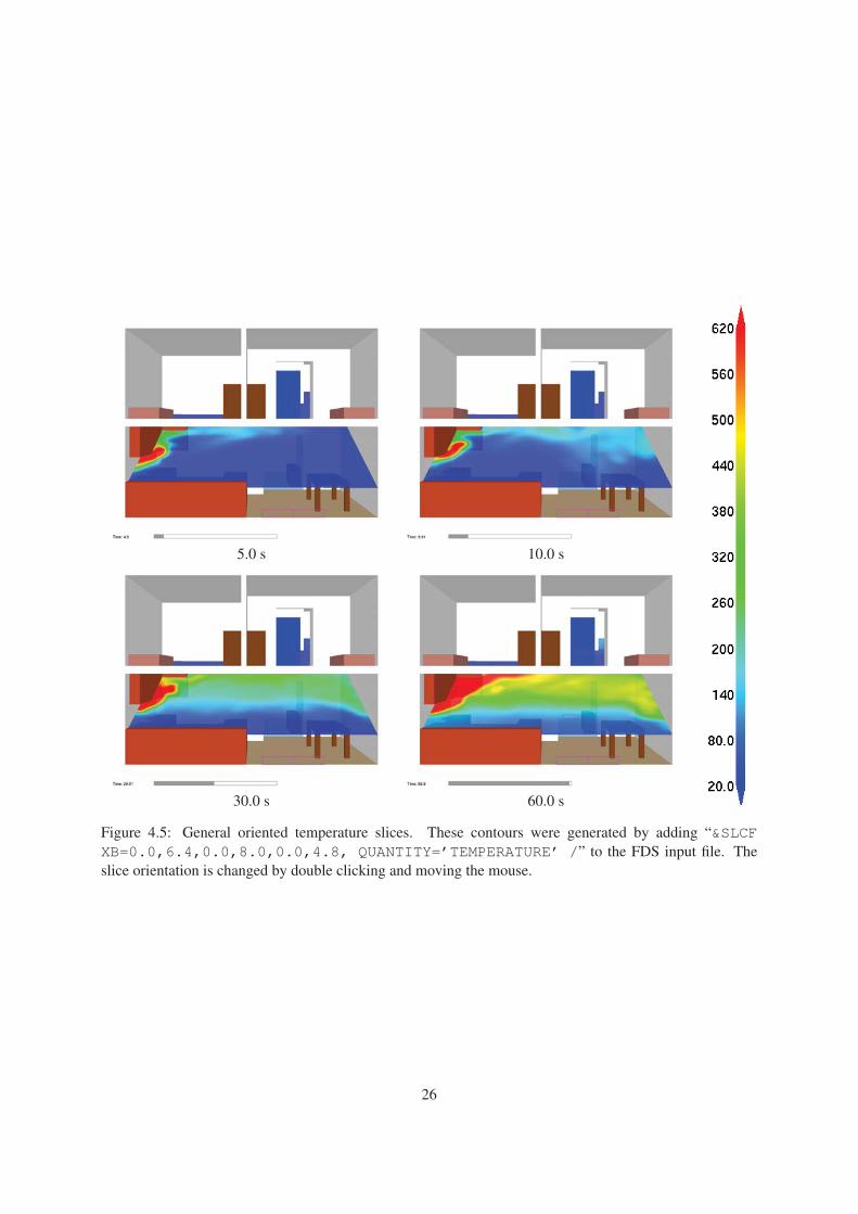
4.5 General oriented temperature slices. . . . . . . . . . . . . . . . . . . . . . . . . . . . . . . 26
4.6 FED slices. . . . . . . . . . . . . . . . . . . . . . . . . . . . . . . . . . . . . . . . . . . . 27
4.7 Boundary file snapshots of shaded wall temperatures contours (cell averaged data). . . . . . 28
4.8 Boundary file snapshots of truncated shaded wall temperatures contours (cell averaged data). 29
4.9 Boundary file snapshots of shaded wall temperatures contours (cell centered data). . . . . . 30
4.10 Isosurface file snapshots of temperature levels. . . . . . . . . . . . . . . . . . . . . . . . . 31
4.11 FED slices. . . . . . . . . . . . . . . . . . . . . . . . . . . . . . . . . . . . . . . . . . . . 33
4.12 Devices dialog box. . . . . . . . . . . . . . . . . . . . . . . . . . . . . . . . . . . . . . . . 33
4.13 Plot3D contour and vector plot examples. . . . . . . . . . . . . . . . . . . . . . . . . . . . 34
4.14 Plot3D isocontour example. . . . . . . . . . . . . . . . . . . . . . . . . . . . . . . . . . . . 35
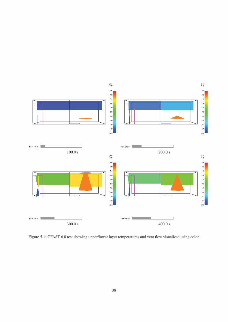
5.1 CFAST 6.0 test showing upper/lower layer temperatures and vent flow visualized using color. 38
5.2 CFAST 6.0 test showing upper/lower layer temperatures and vent flow. Layers are visualized
realistically and vent flow is visualized using color. . . . . . . . . . . . . . . . . . . . . . . 39
6.1 File/Bounds dialog box showing PLOT3D file options. . . . . . . . . . . . . . . . . . . . . 44
6.2 File/Bounds dialog box showing slice and boundary file options. . . . . . . . . . . . . . . . 45
6.3 Ceiling Jet Visualization. . . . . . . . . . . . . . . . . . . . . . . . . . . . . . . . . . . . . 46
6.4 Dialog Box for setting 3D smoke options . . . . . . . . . . . . . . . . . . . . . . . . . . . 47
6.5 Dialog Box for setting miscellaneous Smokeview scene properties. . . . . . . . . . . . . . . 49
6.6 Stereo pair view of a townhouse kitchen fire. . . . . . . . . . . . . . . . . . . . . . . . . . . 50
6.7 Red/blue stereo pair view of a townhouse kitchen fire. . . . . . . . . . . . . . . . . . . . . . 51
6.8 Red/cyan stereo pair view of a townhouse kitchen fire. . . . . . . . . . . . . . . . . . . . . 52
6.9 Dialog box for activating the stereo view option. . . . . . . . . . . . . . . . . . . . . . . . . 52
6.10 Clipping dialog box. . . . . . . . . . . . . . . . . . . . . . . . . . . . . . . . . . . . . . . 53
xiii

6.11 Clipping a scene. . . . . . . . . . . . . . . . . . . . . . . . . . . . . . . . . . . . . . . . . 54
7.1 Object file format. . . . . . . . . . . . . . . . . . . . . . . . . . . . . . . . . . . . . . . . . 57
7.2 Instructions for drawing a sensor along with the corresponding Smokeview view. . . . . . . 58
7.3 Instructions for drawing an inactive and active heat detector along with the corresponding
Smokeview view. . . . . . . . . . . . . . . . . . . . . . . . . . . . . . . . . . . . . . . . . 59
7.4 Instructions for drawing the dynamic object, ball, along with the corresponding FDS input
lines and the Smokeview view. . . . . . . . . . . . . . . . . . . . . . . . . . . . . . . . . . 60
7.5 Smokeview view of several objects defined the objects.svo file. . . . . . . . . . . . . . . . . 61
8.1 Overhead view of the townhouse example showing the default Circle tour and a user defined
tour. . . . . . . . . . . . . . . . . . . . . . . . . . . . . . . . . . . . . . . . . . . . . . . . 70
8.2 Touring dialog boxes. . . . . . . . . . . . . . . . . . . . . . . . . . . . . . . . . . . . . . . 71
8.3 Tutorial examples for Tour option. . . . . . . . . . . . . . . . . . . . . . . . . . . . . . . . 73
9.1 Script Dialog Box. . . . . . . . . . . . . . . . . . . . . . . . . . . . . . . . . . . . . . . . 76
9.2 Script commands generated using the Smokeview script recorder option. . . . . . . . . . . . 77
9.3 Smokeview images generated using script detailed in Figure 9.2 . . . . . . . . . . . . . . . 78
9.4 Script commands generated using the Smokeview script recorder option. . . . . . . . . . . . 81
9.5 Smokeview images generated using script detailed in Figure 9.4 . . . . . . . . . . . . . . . 82
10.1 Colorbar Examples . . . . . . . . . . . . . . . . . . . . . . . . . . . . . . . . . . . . . . . 90
10.2 Colorbar Editor dialog box. . . . . . . . . . . . . . . . . . . . . . . . . . . . . . . . . . . . 91
11.1 Demonstrator dialog box. . . . . . . . . . . . . . . . . . . . . . . . . . . . . . . . . . . . . 94
12.1 Texture map example. . . . . . . . . . . . . . . . . . . . . . . . . . . . . . . . . . . . . . . 96
13.1 Examine Blockages Dialog Box. . . . . . . . . . . . . . . . . . . . . . . . . . . . . . . . . 98
15.1 Ticks Dialog Box. . . . . . . . . . . . . . . . . . . . . . . . . . . . . . . . . . . . . . . . . 102
15.2 Annotation example using the Ticks dialog box . . . . . . . . . . . . . . . . . . . . . . . . 102
15.3 TICKS and LABEL commands used to create image in Figure 15.4 . . . . . . . . . . . . . 103
15.4 Annotation example using the TICKS and LABEL keyword. . . . . . . . . . . . . . . . . . 104
16.1 Compress Files and Autoload dialog box. . . . . . . . . . . . . . . . . . . . . . . . . . . . 106
B.1 Main Menu. . . . . . . . . . . . . . . . . . . . . . . . . . . . . . . . . . . . . . . . . . . . 120
B.2 Load/Unload Menu. . . . . . . . . . . . . . . . . . . . . . . . . . . . . . . . . . . . . . . . 120
B.3 Show/Hide Menu. . . . . . . . . . . . . . . . . . . . . . . . . . . . . . . . . . . . . . . . . 122
B.4 Geometry Menu. . . . . . . . . . . . . . . . . . . . . . . . . . . . . . . . . . . . . . . . . 122
B.5 Label Menu. . . . . . . . . . . . . . . . . . . . . . . . . . . . . . . . . . . . . . . . . . . . 124
B.6 Data Coloring Menu. . . . . . . . . . . . . . . . . . . . . . . . . . . . . . . . . . . . . . . 124
B.7 Option Menu. . . . . . . . . . . . . . . . . . . . . . . . . . . . . . . . . . . . . . . . . . . 127
B.8 Render Menu. . . . . . . . . . . . . . . . . . . . . . . . . . . . . . . . . . . . . . . . . . . 128
B.9 Tour Menu. . . . . . . . . . . . . . . . . . . . . . . . . . . . . . . . . . . . . . . . . . . . 129
B.10 Dialogs Menu. . . . . . . . . . . . . . . . . . . . . . . . . . . . . . . . . . . . . . . . . . . 130
D.1 Example Smokeview rendering using .fds and .GE1 files generated by DXF2FDS. Blockage
and CAD representation of the scene may be toggled by pressing the ‘q’ key. . . . . . . . . 159
xiv

List of Tables
2.1 Keyboard mappings for eye centered or first person scene movement. . . . . . . . . . . . . . 15
D.1 Descriptions of parameters used by the Smokeview OBST keyword. . . . . . . . . . . . . . 153
D.2 Descriptions of parameters used by the Smokeview VENT keyword. . . . . . . . . . . . . . 155
xv

xvi

Part I
Using Smokeview
1


Chapter 1
Introduction
1.1 Overview
Smokeview is a scientific software tool designed to visualize numerical predictions generated by fire models
such as the Fire Dynamics Simulator (FDS), a computational fluid dynamics (CFD) model of fire-driven
fluid flow [1] and CFAST, a zone model of compartment fire phenomena [2]. This report documents version
6 of Smokeview. For details on setting up and running FDS cases read the FDS User’s guide [3].
FDS and Smokeview are used to model and visualize time-varying fire phenomena. However, FDS
and Smokeview are not limited to fire simulation. For example, one may use FDS and Smokeview to
model other applications such as contaminant flow in a building. Smokeview performs this visualization
by displaying time dependent tracer particle flow, animated contour slices of computed gas variables and
surface data. Smokeview also presents contours and vector plots of static data anywhere within a simulation
scene at a fixed time. Several examples using these techniques to investigate fire incidents are documented
in Refs. [4, 5, 6, 7].
Smokeview is used before, during and after model runs. Smokeview is used in a post-processing step to
visualize FDS data after a calculation has been completed. Smokeview may also be used during a calculation
to monitor a simulation’s progress and before a calculation to setup FDS input files more quickly, one can
then use Smokeview to edit or create blockages by specifying the size, location and/or material properties.
Figure 1.1 gives an overview of how data files used by FDS, Smokeview and Smokezip, a program used
to compress FDS generated data files, are related. A typical procedure for using FDS and Smokeview is to:
1. Set up an FDS input file.
2. Run FDS. FDS then creates one or more output files interpreted by Smokeview to visualize the calcu-
lation results.
3. Run Smokeview to analyze the output files generated by step 2. by either double-clicking the file
named casename.smv with the mouse (on the PC) or by typing smokeview casename at a
command line. Smokeview may also be used to create new blockages and modify existing ones. The
blockage changes are saved in a new FDS input data file.
This publication documents step 3. Steps 1 and 2 are documented in the FDS User’s Guide [3].
Menus in Smokeview are activated by clicking the right mouse button anywhere within the Smokeview
window. Data files may be visualized by selecting the desired Load/Unload menu option. Other
menu options are discussed in Appendix B. Many menu commands have equivalent keyboard shortcuts.
These shortcuts are listed in Smokeview’s Help menu and are described in Appendix C. Visualization
3

SmokeviewInput (.smv) Smokezip
Config(.ini)
Boundary (.bf),3d smoke (.s3d),Particle (.prt5),
Slice/vector (.sf),Iso-surface (.iso)
Input(.fds)
Smokeview
FDS
Plot3D (.q)
Boundary (.bf.svz),3d smoke (.s3d.svz),Particle (.part.svz),
Slice/vector (.sf.svz),Iso-surface (.iso.svz)
Compressed
Display
devc (.csv)hrr (.csv)
Figure 1.1: Diagram illustrating files used and created by the Fire Dynamics Simulator (FDS), Smokezip
and Smokeview.
features not controllable through the menus may be customized by using the Smokeview preference file,
smokeview.ini , discussed in Appendix D.3.
Smokeview is written in C [8] and Fortran 90 [9] and consists of about 100,000 lines of code. The C por-
tion of Smokeview visualizes the data, while the Fortran 2003 portion reads in data generated by FDS (also
written in Fortran 2003). Smokeview uses the 3D graphics library OpenGL [10] and the Graphics Library
Utility Toolkit (GLUT) [11]. Smokeview uses the GLUT software library so that most of the development
effort can be spent implementing the visualizations rather than creating an elaborate user interface. Smoke-
view uses a number of auxiliary libraries to implement image capture (GD [12, 13], PNG [14], JPEG [15]),
image and general file compression (ZLIB [16]) and dialog creation (GLUI [17]). Each of these libraries is
portable running under UNIX, LINUX, OSX and Windows 9x/2000/XP/Vista allowing Smokeview to run
on these platforms as well.
1.2 Features
Smokeview is a program designed to visualize numerical calculations generated by the Fire Dynamics Sim-
ulator. The version of FDS used to run the cases illustrated in this report is given by:
Fire Dynamics Simulator
Version: 6.0.0; MPI Disabled; OpenMP DisabledSVN Revision Number: 10896Compile Date: Mon, 04 Jun 2012
4

Consult FDS Users Guide Chapter, Running FDS, for further instructions.
Hit Enter to Escape...
The version of Smokeview described here and used to generate most figures in this report is given by:
Smokeview 6.0.1 - Jun 20 2012
Version: 6.0.1Smokeview (64 bit) Revision Number: 11112Platform: WIN64 (MSVS C/C++)Build Date: Jun 20 2012Smokeview path: c:\Program Files\FDS\FDS5\bin\smokeview_win_64Smokezip path: c:\Program Files\FDS\FDS5\bin\smokezip_win_64.exe
1.2.1 Visualizing Data
Smokeview visualizes data primarily generated by FDS. Smokeview visualizes data that is both dynamic
and static. Dynamic data is visualized by animating particle flow (showing location and values of tracer
particles), 2D contour slices (both within the domain and on solid surfaces) and 3D iso surfaces. 2D contour
slices can also be drawn with colored vectors that use velocity data to show flow direction, speed and value.
Static data is visualized similarly by drawing 2D contours, vector plots and 3D level surfaces.
Particles
Lagrangian or moving particles can be used to visualize the flow field. Often these particles represent smoke
or water droplets.
Particle data may also be visualized as streak lines (a particle drawn where it has been for a short period
of time in the past). Streak lines are a good method for displaying motion with still pictures.
Slices - 2D contours
Animated 2D shaded color contour plots are used to visualize gas phase information, such as temperature
or density. The contour plots are drawn in horizontal or vertical planes along any coordinate direction.
Contours can also be drawn in shades of grey.
Animated 2D shaded color contour plots are also used to visualize solid phase quantities such as radia-
tive flux or heat release rate per unit area.
Vector slice files may be visualized if U, V and W velocity slice files are recorded. Though similar
to solidly shaded contour animations (the vector colors are the same as the corresponding contour colors),
vector animations are better than solid contour animations for highlighting flow features since vectors ac-
centuate the direction that flow is occuring.
A 3D region of data may be visualized using slice files. Slices may be moved from one plane to the next
just as with PLOT3D files (using up/down cursor keys or page up/page down keys). 3D slices may also be
rotated and/or translated by double clicking and moving the mouse. If the ALT key is also pressed, the slice
moves up and down. If the CTRL key is pressed the slice moves side to side. Otherwise, the slice rotates.
Data for 3D slice files are generated by specifying a 3D rather than a 2D region with the &SLCF keyword.
Data computed at cell centers rather than interpolated at cell nodes may be visualized. This is useful for
investigating numerical algorithms as the data visualized has not been interpolated before being seen.
5

Surfaces - 3D contours
Isosurface or 3D level surface animations may be used to represent flame boundaries, layer interfaces and
various other gas phase variables. Multiple isocontours may be stored in one file, allowing one to view
several isosurface levels simultaneously.
Volumetric - Realistic Smoke
Smoke and fire (heat release rate per unit volume) are displayed realistically using a series of partially
transparent planes. The smoke transparencies are determined by using smoke densities computed by FDS.
The fire and sprinkler spray transparencies are determined by using a heuristic based on heat release rate
and water density data, again computed by FDS. Various settings for the 3D smoke option may be set using
the 3D Smoke dialog box found in the Dialogs menu. The windows version of Smokeview uses the
graphical processing unit (GPU) on the video card to perform some of the calculations required to visualize
smoke.
1.2.2 Exploring Data
Data Mining
The user can analyze and examine the simulated data by altering its appearance to more easily identify
features and behaviors found in the simulation data. One may flip or reverse the order of colors in the
colorbar and also click in the colorbar and slide the mouse to highlight data values in the scene. These
options may be found under Options/Shades .
The user may click in the time bar and slide the mouse to change the simulation time displayed. One use
for the time bar and color bar selection modes might be to determine when smoke of a particular temperature
enters a room.
Data Filtering
The File/Bounds Settings... dialog box allows one to set bounds, to chop or hide data and in the case of
slice file data to time average. The data chopping feature is useful for highlighting data. A ceiling jet, for
example, may be visualized by hiding ambient temperature data, data below a prescribed temperature. Using
time averaging allows one to smooth noisy data over a user selectable time interval.
Data coloring
Multiple colorbars are available for displaying simulation data. New colorbars may be created using the
colorbar editor. Colorbars may then be adapted to best highlight the simulation data visualized. Regions in
the simulation with certain data values may be highlighted by clicking on the colorbar.
Data Compression
- An option has been added to the LOAD/UNLOAD menu to compress 3D smoke and boundary files. The
option shells out to the program smokezip which runs in the background enabling one to continue to use
Smokeview while files are compressing.
6

1.2.3 Exploring the Scene
Motion/View
The motion/view dialog box may be used to allow more precise control of scene movement and orienta-
tion. Cursor keys have been mapped to scene translation/rotation to allow easy navigation within the scene.
Viewpoints may be saved for later access.
The first person or eye view mode for moving allows one to move through a scene more realistically.
Using the cursor keys and the mouse, one can move through a scene virtually.
Scene Clipping
It is often difficult to visualize data in complicated geometries due to the number of obstructed surfaces.
Interior portions of the scene may be seen more easily by clipping part of the scene away.
Clipping discussed above occurs in 3D within the scene. A screenshot converted to a PNG or JPEG file
may also be clipped or cropped using the Render portion of the Motion/View/Render dialog box.
Stereo views
A method for displaying stereo/3D images has been implemented that does not require any specialized
equipment such as shuttered glasses or quad buffered enabled video cards. Stereo pair images are displayed
side by side after invoking the option with the Stereo dialog box or pressing the ”S” key (upper case). A 3D
view appears by relaxing the eyes, allowing the two images to merge into one. Pressing the ”S” key again
results in stereo views generated by displaying red and blue versions of the scene. Glasses with a red left
lens and a blue right lens are required to view the image.
1.2.4 Customizing the Scene
Objects
A method for drawing objects (an object being a heat detector, smoke detector, sprinkler sensor etc.) has
been implemented in Smokeview 5. These objects look more realistic. Objects are specified in a data file
rather than in Smokeview as C code. This allows one to customize the look and feel of the objects (to match
the types of detectors/sprinklers that are being used) without requiring code changes in Smokeview.
Annotating Cases
The LABEL keyword is used to help document Smokeview output. It allows one to place colored labels at
specified locations at specified times. A second keyword, TICK keyword places equally spaced tick marks
between specified bounds. These marks along with LABEL text may be used to specify length scales in the
scene.
The User Tick Settings tab of the Display dialog box provides an easier way to place ticks with length
annotations along coordinate axes.
Texture Mapping
JPEG or PNG image files may be applied to a blockage, vent or enclosure boundary. This is called texture
mapping. This allows Smokeview scenes to appear more realistic. These image files may be obtained from
the internet, a digital camera, a scanner or from any other source that generates these file formats. Image
files used for texture mapping should be seamless. A seamless texture as the name suggests is periodic in
7

both horizontal and vertical directions. This is an especially important requirement when textures are tiled
or repeated across a blockage surface.
1.2.5 Automating the Visualization
Scripting
Smokeview may be run in an unattended mode using instructions found in a script file. These instructions
direct Smokeview to load data files, load configuration files, set view points and time values in order to
document a case by rendering the Smokeview scene into one or more image files. The script file may be
created by Smokeview as a user performs various actions or may be created by editing a text file.
Virtual Tour
A series of checkpoints or key frames specifying position and view direction may be specified. A smooth
path is computed using Kochanek-Bartels splines [18] to go through these key frames so that one may
control the position and view direction of an observer as they move through the simulation. One can then
see the simulation as the observer would. This option is available under the Tour menu item. Existing
tours may be edited and new tours may be created using the Tour dialog box found in the Dialogs menu.
Tour settings are stored in the local configuration file (casename.ini).
1.3 Getting Started
1.3.1 Obtaining Smokeview
Smokeview is available at http://fire.nist.gov/fds . This site contains links to various instal-
lation packages for different operating systems. It also contains documentation for Smokeview and FDS,
sample FDS calculations, software updates and links for requesting feedback about the software.
After obtaining the setup program, install Smokeview on the PC by either entering the setup program
name from the Windows Start/Run... menu or by double-clicking the downloaded Smokeview setup pro-
gram. The setup program then steps through the program installation. It copies the FDS and Smokeview
executables, sample cases, documentation and the Smokeview preference file smokeview.ini to the a
default directory. The setup program also defines PATH variables and associates the .smv file extension
to the Smokeview program so that one may either type Smokeview at any command line prompt or dou-
ble click on any .smv file. Smokeview uses the OpenGL graphics library which is a part of all Windows
distributions.
Most computers purchased today are perfectly adequate for running Smokeview. For Smokeview it
is more important to obtain a fast graphics card than a fast CPU. If the computer will run both FDS and
Smokeview then it is important to obtain a fast CPU as well. For example, the townhouse case used for
many examples in this report consists of about 180000 grid cells and is used in many of the Figures in this
report, required about 1.2 CPU hours on a 2.0 GHZ Intel Core i7-2630QM Windows 7 system. Cases with
more grid cells and longer simulation times (the townhouse case simulated 300 s of smoke flow) would
clearly benefit from a faster CPU and more memory which are now relatively inexpensive.
1.3.2 Running Smokeview
Smokeview may be started on the PC by double-clicking the file named casename.smv where casename
is the name specified by the CHID keyword defined in the FDS input data file. Menus are accessed by
clicking with the right mouse button. The Load/Unload menu may be used to read in the data files
8

to be visualized. The Show/Hide menu may be used to change how the visualizations are presented.
For the most part, the menu choices are self explanatory. Menu items exist for showing and hiding various
simulation elements, creating screen dumps, obtaining help etc. Menu items are described in Appendix B.
To use Smokeview from a command line, open a command shell. Then change to the directory contain-
ing the FDS case to be viewed and type:
smokeview casename
where again casename is the name specified by the CHID keyword defined in the FDS input data file.
Data files may be loaded and options may be selected by clicking the right mouse button and picking the
appropriate menu item.
Smokeview opens two windows, one displays the scene and the other displays status information. Clos-
ing either window will end the Smokeview session. Multiple copies of Smokeview may be run simultane-
ously if the computer has adequate resources.
Normally Smokeview is run during an FDS run, after the run has completed and as an aid in setting up
FDS cases by visualizing geometric components such as blockages, vents, sensors, etc. One can then verify
that these modelling elements have been defined and located as intended. One may select the color of these
elements using color parameters in the smokeview.ini to help distinguish one element from another.
smokeview.ini file entries are described in section D.3.
Although specific video card brands cannot be recommended, they should be high-end due to Smoke-
view’s intensive graphics requirements. These requirements will only increase in the future as more features
are added. A video card designed to perform well for fancy computer games should do well for Smokeview.
Some apparent bugs in Smokeview have been found to be the result of problems found in video cards on
older computers.
9

10

Chapter 2
Manipulating the Scene
The scene may be manipulated from two points of view, a world or global view and a first person or eyeview. These views may be switched by pressing the “e” key or by selecting the appropriate radio button in
the Motion/View dialog box.
2.1 World View
The scene may be rotated or translated while in world view, either directly with the mouse or by using con-
trols contained in the Motion/View/Render dialog box. This dialog box is opened from the Dialogs>Motion/View/Render
menu item and is illustrated in Figure 2.1.
Clicking on the scene and dragging the mouse horizontally, vertically or a combination of both results
in scene rotation or translation depending upon whether the left, middle or right mouse button is depressed.
left mouse button horizontal and vertical mouse motion results in scene rotation.
middle mouse button Horizontal mouse movement when the middle mouse button is depressed results
in scene translation from side to side along the X axis. Vertical mouse movement results in
scene translation into and out of the computer screen along the Y axis. Alternatively, one can
depress the CTRL key and the left mouse button to achieve the same effect.
right mouse button Vertical mouse movement when the right mouse button is depressed results in verti-
cal scene translation along the Z axis. Horizontal mouse movement has no effect. Alternatively,
one can depress the ALT key and the left mouse button to achieve the same effect. Note that the
right mouse button is also used to display Smokeview menus. To switch this behavior to scene
movement, press the M key. Press the M key again to switch back to menu use.
The Motion/View/Render dialog box, illustrated in Figure 2.1 may be used to move the scene in a more
controlled manner. For example, buttons in the Motion region allows one to translate or rotate the scene.
The Horizontal button allows one to translate the scene horizontally in a left/right or in/out direction
while the Vertical button allows one to translate the scene in an up/down direction.
Controls in the Window Properties region of the Motion/View/Render dialog box allow one to change
the scene magnification or zoom factor and the projection method used to draw objects (perspective or size
preserving). These two projection methods differ in how objects are displayed at a distance. A perspective
projection for-shortens or draws an object smaller when drawn at a distance. An isometric or size preserving
projection on the other hand draws an objects the same size regardless of where it is drawn in the scene.
11

Figure 2.1: Motion/View Dialog/Render Box - Motion, Window Properties and Viewpoint Regions. Rotate
or translate the scene by clicking an arrow and dragging the mouse. The Motion/View/Render Dialog Box
is invoked by selecting Dialogs>Motion/View/Render .
12

Figure 2.2: Motion/View Dialog/Render Box. Render and Scaling/Depth regions.
13

Controls in the Render and Scaling Depth regions, as illustrated in Figure 2.2, allow one to render
images using either PNG or JPEG file formats and to scale the Smokeview scene (say for visualizing tunnel
scenarios) in any or all of the coordinate directions.
The zoom and aperture edit boxes allow one to change the magnification of the scene or equiva-
lently the angle of view across the scene. The relation between these two parameters is given by
zoom = tan(45◦/2)/ tan(aperture/2)
A default aperture of 45◦ is chosen so that Smokeview scenes have a normal perspective.
View may be used to reset the scene back to either an external, internal (to the scene), or previously
saved viewpoint.
Rotate about A pull down list appears in multi-mesh cases allowing one to change the rotation center.
Therefore one could rotate the scene about the center of the entire physical domain or about the
center of any one particular mesh. This is handy when meshes are defined far apart.
Rotation Buttons Rotation buttons are enabled or disabled as appropriate for the mode of scene motion.
For example, if about world center - level rotations has been selected, then the Rotate X
and Rotate eye buttons are disabled. A rotation button labeled 90 deg has been added
to allow one to rotate 90 degrees while in eye center mode. This is handy when one wishes to
move down a long corridor precisely parallel to one of the walls. The first click of 90 deg snaps
the view to the closest forward or side direction while each additional click rotates the view 90
degrees clockwise.
View Buttons A viewpoint is the combination of a location and a view direction. Several new buttons
have been added to this dialog box to save and restore viewpoints. The scene is manipulated to
the desired orientation then stored by pressing the Add button which adds the new viewpoint
or the Replace button which replaces this viewpoint with the currently selected one. To change
the view to a currently stored viewpoint, use the Select listbox to select the desired viewpoint.
The Delete button may be used to remove a viewpoint from the stored list. The View name text
box may be used to change the name or label for the selected viewpoint. The view at startupbutton is used to specify the viewpoint that should be set when Smokeview first starts up.
2.2 Eye View
Radio buttons in the Motion/View dialog box allow one to toggle between world, eye centered and world
level rotation scene movement modes. These modes may also be changed by using the “e” key. When in
eye center mode, several key mappings have been added, inspired by popular computer games, to allow for
easier movement within the scene. For example, the up and down cursor keys allow one to move forward
or backwards. The left and right cursor keys allow one to rotate left or right. Other keyboard mappings are
described in Table 2.1.
14

Table 2.1: Keyboard mappings for eye centered or first person scene movement.
Key Description
up/down cursormove forward/backward
w/s
ALT + left/right cursorslide left/right
a/dALT + up/down cursor move up/down
left/right cursor rotate left/right
Page Up/Down look up/down
Home look level
Pressing the SHIFT key while moving, sliding or rotating
results in a 4x speedup of these actions.
15

16

Chapter 3
Visualizing Smoke
3.1 Tracers and Streaklines
Particle files contain the locations of tracer particles used to visualize the flow field. Figure 3.1 shows several
snapshots of a developing kitchen fire visualized by using particles where particles are colored black. If
present, sprinkler water droplets would be colored blue. Particles are stored in files ending with the extension
.prt51 and are displayed by selecting the particle file entry from the Load/Unload menu.
Streaklines are a technique for showing motion in a still image. Figure 3.2 shows a snapshot of the same
kitchen fire using streak lines instead of particles. The streaks begin at 6 s and end at 10 s.
Particle file data may be converted to an isosurace using Smokezip. The isosurface location is defined in
terms of particle density and the isosurface color is defined in terms of averaged particle values. See Chapter
16.1 for more details on using Smokezip for generating isosurface files from particle files and Section ?? for
some examples.
3.2 Realistic
FDS generates several data files visualized by Smokeview. Each file type may be loaded or unloaded using
the Load/Unload menu described in Appendix B.2. Visualizations produced by these data files are
described in this and the following sections. The format used to store each of the data files is given in the
FDS User’s Guide [3].
Visualizing smoke realistically is a daunting challenge for at least three reasons. First, the storage
requirements for describing smoke can easily exceed the disk capacities of present 32 bit operating systems
such as Linux, i.e. file sizes can easily exceed 2 gigabytes. Second, the computation required both by the
CPU and the video card to display each frame can easily exceed 0.1 s, the time corresponding to a 10 frame/s
display rate. Third, the physics required to describe smoke and its interactions with itself and surrounding
light sources is complex and computationally intensive. Therefore, approximations and simplifications are
required to display smoke rapidly.
Smoke visualization techniques such as tracer particles or shaded 2D contours are useful for quantitative
analysis but not suitable for virtual reality applications, where displays need to be realistic and fast as well as
accurate. The approach taken by Smokeview is to display a series of parallel planes. Each plane is colored
black (for smoke) with transparency values pre-computed by FDS using time dependent soot densities also
computed by FDS corresponding to the grid spacings of the simulation. The transparencies are adjusted
1Particle files created with FDS version 4 and earlier use the .part extension
17

5.0 s 10.0 s
30.0 s 60.0 s
Figure 3.1: Townhouse kitchen fire visualized using tracer particles.
18

Figure 3.2: Townhouse kitchen fire visualized using streak lines. The pin heads shows flow conditions at
10 s, the corresponding tails shows conditions 0.25 s.
19

5.0 s 10.0 s
30.0 s 60.0 s
Figure 3.3: Smoke3d file snapshots at various times in a simulation of a townhouse kitchen fire.
in real time by Smokeview to account for differing path lengths through the smoke as the view direction
changes. The graphics hardware then combines the planes together to form one image.
Fire by default is colored a dark shade of orange wherever the computed heat release rate per unit volume
exceeds a user-defined cutoff value. The visual characteristics of fire are not automatically accounted for.
The user though may use the 3D Smoke dialog box to change both the color and transparency of the fire for
fires that have non-standard colors and opacities.
The windows version of Smokeview has the option of using the GPU or graphics programming unit to
perform some of the calculations required to visualize realistic smoke. These calculations consist of adjust-
ing the smoke opaqueness as pre-computed in FDS to account for off-axis viewing directions. The GPU
performs the computations in parallel while the former method using the CPU performs them sequentially.
For many (but not all) cases, the use of the GPU results in a smoke drawing speed up of 50 % or more. This
option is turned on or off by pressing the G key.
Figure 3.3 illustrates a visualization of realistic smoke.
20

Chapter 4
Visualizing Data Quantitatively
4.1 2D Shaded Contours and Vector Slices - Slice Files
4.1.1 Axis aligned slices
Slice files contain results recorded within a rectangular array of grid points at each recorded time step.
Continuously shaded contours are drawn for simulation quantities such as temperature, gas velocity and
heat release rate. Figure 4.1 shows several snapshots of a vertical animated slice where the slice is colored
according to gas temperature. Slice files have file names with extension .sf and are displayed by selecting
the desired entry from the Load/Unload menu.
To specify in FDS a vertical slice 1.5 m from the y = 0 boundary colored by temperature, use the line:
&SLCF PBY=1.5 QUANTITY=’TEMPERATURE’ /
A more complete list of output quantities may be found in Ref. [3].
Vector slices Animated vectors are displayed using data contained in two or more slice files. The direction
and length of the vectors are determined from the U , V and/or W velocity slice files. The vector colors are
determined from the file (such as temperature) selected from the Load/Unload menu. The length of
the vectors can be adjusted by pressing the ‘a’ key. For cases with a fine grid, the number of vectors may
be overwhelming. Vectors may be skipped by pressing the ‘s’ key. Figure 4.2 shows a sequence of vector
slices corresponding to the shaded temperature contours found in Figure 4.1.
To generate the extra velocity files needed to view vector animations, add VECTOR=.TRUE. to the
above &SLCF line to obtain:
&SLCF PBY=1.50,QUANTITY=’TEMPERATURE’,VECTOR=.TRUE. /
Data coloring Smokeview uses a 1D texture map for coloring data occurring in slice, boundary and
PLOT3D files. This is illustrated in Figure 4.3. The colors are now crisper and sharper, more accurately
representing the underlying data. This is most noticeable when selecting the colorbar with the mouse. As
before this causes a portion of the colorbar to turn black and the corresponding region in the scene to also
turn black. Now the black color is accurate to the pixel so this feature could be used to highlight regions of
interest. The improved accuracy is a result of the way color interpolations are performed. Colors are inter-
polated within the colorbar using a 1D texture map. Color interpolations with the former method occurred
within the color cube.
21

5.0 s 10.0 s
30.0 s 60.0 s
Figure 4.1: Slice file snapshots of shaded temperature contours at various times in a simulation. These
contours were generated by adding “&SLCF PBY=1.5, QUANTITY=’TEMPERATURE’ /” to the FDS
input file.
22

5.0 s 10.0 s
30.0 s 60.0 s
Figure 4.2: Vector slice file snapshots of shaded vector plots. These vector plots were generated by using
“&SLCF PBY=1.5,QUANTITY=’TEMPERATURE’,VECTOR=.TRUE. /”.
23

colors interpolated using a 3D color cube colors interpolated using a 1D texture color bar
Figure 4.3: Slice file snapshots illustrating old and new method for coloring data.
24

Figure 4.4: Motion/View/Render Dialog Box - General slice regions.
4.1.2 3D slices
The user may visualize a 3D region of data using slice files. To specify a cube of data from 1.0 to 2.0 in
each of the X, Y and Z directions in FDS , use the line:
&SLCF XB=1.0,2.0,1.0,2.0,1.0,2.0 QUANTITY=’TEMPERATURE’ /
A slice from the resulting slice file may be moved from one plane to the next just as with PLOT3D
files (using left/right, up/down cursor keys or page up/page down keys). 3D slices may also be oriented
arbitrarily (not aligned with a coordinate axis) as illustrated in Figure 4.5.
A slice may also be oriented in an arbitrary direction. double clicking within the scene. While holding
down the mouse after double clicking, move the mouse from side to side or up and down to rotate the general
slice. Double clicking and moving the mouse vertically while holding down the ALT key causes the center
of rotation for the general slice to move up and down. Double clicking and moving the mouse horizontally
and vertically while holding down the SHIFT key causes the center of rotation for the general slice to move
along the X and Y axis respectively.
General slices may also be oriented using the General slice motion region of the Motion/View/Render
dialog box as illustrated in Figure 4.4.
4.1.3 Fractional effective dose (FED) slices
The fractional effective dose (FED), developed by Purser [19], is a measure of human incapacitation due to
combustion gases. FED index data is computed by Smokeview using CO, CO2 and O2 gas concentration
data computed by FDS. This data is made available to Smokeview in the form of slice files. Smokeview
computes FED data using
FEDtot = FEDCO ×HVCO2+FEDO2
(4.1)
25
5.0 s 10.0 s
30.0 s 60.0 s
Figure 4.5: General oriented temperature slices. These contours were generated by adding “&SLCFXB=0.0,6.4,0.0,8.0,0.0,4.8, QUANTITY=’TEMPERATURE’ /” to the FDS input file. The
slice orientation is changed by double clicking and moving the mouse.
26

5.0 s 10.0 s
30.0 s 60.0 s
Figure 4.6: FED slices. These contours were generated using CO, CO2 and O2 data slices.
where FEDtot is the total FED, FEDCO is the FED due to CO, HVCO2is a hyper-ventilating factor applied to
CO and FEDO2is the FED due to CO2. The species data slices used to compute an FED slice needs to be
specified at the same location. In the following, an FED slice would be computed at y = 1.6.
&SLCF PBY=1.6,QUANTITY=’VOLUME FRACTION’ SPEC_ID=’CARBON DIOXIDE’ /&SLCF PBY=1.6,QUANTITY=’VOLUME FRACTION’ SPEC_ID=’CARBON MONOXIDE’ /&SLCF PBY=1.6,QUANTITY=’VOLUME FRACTION’ SPEC_ID=’OXYGEN’ /
FED computations are stored by Smokeview in slice files for subsequent use. Since this computation is
performed in Smokeview using data only found in the slices files, time step intervals should be chosen to
ensure accuracy. Figure 4.6 illustrates an FED slice file.
4.2 2D Shaded Contours on Solid Surfaces - Boundary Files
Boundary files contain simulation data recorded at blockage or wall surfaces. Continuously shaded con-
tours are drawn for quantities such as wall surface temperature, radiative flux, etc. Figure 4.9 shows sev-
eral snapshots of a boundary file animation where the surfaces are colored according to their temperature.
Boundary files have file names with extension .bf and are displayed by selecting the desired entry from
27

5.0 s 10.0 s
30.0 s 60.0 s
Figure 4.7: Boundary file snapshots of shaded wall temperatures (cell averaged data). These snapshots were
generated by using “&BNDF QUANTITY=’WALL TEMPERATURE’/”.
the Load/Unload menu. Figure 4.8 shows the same snapshots as in Figure 4.9 except that data below
200 ◦Cis chopped.
A boundary file containing wall temperature data may be generated by using:
&BNDF ’WALL_TEMPERATURE’ /
Loading a boundary file is a memory intensive operation. The entire boundary file is read in to determine
the minimum and maximum data values. These bounds are then used to convert four byte floats to one byte
color indices. To drastically reduce the memory requirements, simply specify the minimum and maximum
data bounds using the Set Bounds dialog box. This should be done before loading the boundary file data.
When this is done, memory for the boundary file data is allocated for only one time step rather than for all
time steps.
4.3 3D Contours - Isosurface Files
The surface where a quantity such as temperature attains a given value is called an isosurface. An isosurface
is also called a level surface or 3D contour. Isosurface files contain data specifying isosurface locations for
28

5.0 s 10.0 s
30.0 s 60.0 s
Figure 4.8: Boundary file snapshots of truncated shaded wall temperatures (cell averaged data). Data
values are truncated or chopped below 200 ◦C. These snapshots were generated by using “&BNDFQUANTITY=’WALL TEMPERATURE’/”.
29

5.0 s 10.0 s
30.0 s 60.0 s
Figure 4.9: Boundary file snapshots of shaded wall temperatures (cell centered data) These snapshots were
generated by using “&BNDF QUANTITY=’WALL TEMPERATURE’ CELL CENTERED=.TRUE. /”.
30

5.0 s 10.0 s
30.0 s 60.0 s
Figure 4.10:
Isosurface file snapshots of temperature levels. The orange surface is drawn where the air/smoke temperature
is 30 ◦C and the white surface is drawn where the air/smoke temperature is 100 ◦C. These snapshots were
generated by adding “&ISOF QUANTITY=’TEMPERATURE’,VALUE(1)=30.0,VALUE(2)=100.0/” to the FDS input file.
31

a given quantity at one or more levels. These surfaces are represented as triangles. Isosurface files have
file names with extension .iso and are displayed by selecting the desired entry from the Load/Unloadmenu.
Isosurfaces are specified in the FDS input file with the &ISOF keyword. To specify isosurfaces for
temperatures of 30◦C and 100◦C as illustrated in Figure 4.10 add the line:
&ISOF QUANTITY=’TEMPERATURE’, VALUE(1)=30.0, VALUE(2)=100.0 /
to the FDS input file. A complete list of isosurface quantities may be found in Ref. [3]
4.3.1 Isosurfaces for fractional effective dose data
As with 2D slices, Smokeview computes the fractional effective dose (FED) for isosurfaces if 3D slices for
CO2, CO and O2 are specified in the FDS input file. 3D slices are required to compute isosurfaces. Again,
these slices need to be specified at the same location as in
&SLCF XB=0.0,1.6,0.0,1.6,0.0,3.2,QUANTITY=’VOLUME FRACTION’ SPEC_ID=’CARBON DIOXIDE&SLCF XB=0.0,1.6,0.0,1.6,0.0,3.2,QUANTITY=’VOLUME FRACTION’ SPEC_ID=’CARBON MONOXID&SLCF XB=0.0,1.6,0.0,1.6,0.0,3.2,QUANTITY=’VOLUME FRACTION’ SPEC_ID=’OXYGEN’ /
Figure 4.11 illustrates an FED isosurfaces where the three levels are at 0.3 (blue), 1.0 (yellow) and 3.0 (red).
4.4 Device data - .csv files
Spreadsheet data, generated by either FDS or CFAST or imported from some other source, may be visualized
by Smokeview. Version 6 of both FDS and CFAST both generate spreadsheet files using the same file format
given by
unit1,unit2, ..., unitNlabel1,label2, ..., labelNdata11,data12, ..., data1Ndata21,data22, ..., data2N....datam1,datam2, ..., dataMN
where the unit and label entries are character strings and the data entries are floating point numbers.
FDS uses spreadsheet files to store device and heat release data. CFAST uses spreadsheet files to store
the results of the simulation (room pressures, layer heights, layer temperatures etc.). To view spreadsheet
data generated by FDS, open the Devices/Objects dialog box illustrated in Figure 4.12 and select the “Show
values” checkbox. If U, V and/or W velocity data is contained in the spreadsheet file then velocity vectors
may also be displayed.
4.5 Static Data - Plot3D Files
Data stored in Plot3D files use a format developed by NASA [20] and are used by many CFD programs for
representing simulation results. Plot3D files store five data values at each grid cell. FDS uses Plot3D files
to store temperature, three components of velocity (U, V, W) and heat release rate. Other quantities may be
stored if desired.
An FDS simulation will automatically create Plot3D files at several specified times throughout the sim-
ulation. Plot3D data is visualized in three ways: as 2D contours, vector plots and isosurfaces. Figure 4.13a
32

5.0 s 10.0 s
30.0 s 60.0 s
Figure 4.11: FED isosurfaces. These level surfaces were generated using CO, CO2 and O2 3D data slices.
The blue, yellow and red surfaces represent where the fed values are 0.3, 1.0 and 3.0 respectively.
Figure 4.12: Devices dialog box. This dialog box allows the user to display data values stored in FDS
spreadsheet files.
33

a) shaded 2D temperature contour plots in a
vertical plane through the fire
b) shaded temperature vector plot in a ver-
tical plane through the fire. The “a” key
may be depressed to alter the vector sizes.
The “s” key may be depressed to alter the
number of vectors displayed.
Figure 4.13: Plot3D contour and vector plot examples.
shows an example of a 2D Plot3D contour. Vector plots may be viewed if one or more of the U,V and W
velocity components are stored in the Plot3D file. The vector length and direction show the direction and
relative speed of the fluid flow. The vector colors show a scalar fluid quantity such as temperature. Figure
4.13b shows vectors. The vector lengths may be adjusted by depressing the “a” key. Figure 4.14 gives an
example of isosurfaces. Plot3D data are stored in files with extension .q .
34

a) temperature isosurface at 350 ◦C b) temperature isosurface at 530 ◦C
Figure 4.14: Plot3D isocontour example.
35

36

Chapter 5
Visualizing Zone Fire Data
Smokeview may be used to visualize data simulated by a zone fire model. The zone fire model, CFAST [2],
creates data files containing geometric information such as room dimensions and orientation, vent locations
etc.. It also outputs modeling quantities such as pressure, layer interface heights, and lower and upper
layer temperatures. Smokeview visualizes the geometric layout of the scenario. It also visualizes the layer
interface heights, upper layer temperature and vent flow. Vent flow is computed internally in Smokeview
using the same equations and data as used by CFAST. For a given room, pressures , Pi, are computed at a
number of elevations, hi using
Pi = Pf −ρLgmin(hi,yL)−ρU gmax(hi − yL,0)
where Pf is the pressure at the floor (relative to ambient), ρL and ρU are the lower and upper layer densities
computed from layer temperatures using the ideal gas law and g is the acceleration of gravity. When densities
vary continuously with height, this becomes Pi = Pf −∫ h
0 ρ(z)gdz. A pressure difference profile is then
determined using pressures computed on both sides of the given vent.
In the visualization, colors represent the gas temperature of the vent flow. The colors change because the
flow may come from either the lower (cooler) or upper (hotter) layer. The length and direction of the colored
vent flow region represents a vent flow speed and direction. Plumes are represented as inverted cones with
heights calculated in Smokeview using the same correlation as CFAST and heat release rate data computed
by CFAST. A Smokeview view of the one room sample case that comes with the CFAST installation is
illustrated in Figures 5.1 and 5.2.
37
100.0 s 200.0 s
300.0 s 400.0 s
Figure 5.1: CFAST 6.0 test showing upper/lower layer temperatures and vent flow visualized using color.
38

100.0 s 200.0 s
300.0 s 400.0 s
Figure 5.2: CFAST 6.0 test showing upper/lower layer temperatures and vent flow. Layers are visualized
realistically and vent flow is visualized using color.
39

40

Part II
Controlling and Customizing Smokeview
41


Chapter 6
Setting Options
6.1 Setting Data Bounds
Normally, Smokeview determines data bounds automatically when it loads data. Sometimes, however, it is
desirable to override Smokeview’s choice. This allows for consistent color shading when displaying several
data files simultaneously.
The File/Bounds... dialog box is opened from the Dialogs menu. Each file type in Figure 6.1 (slice,
particle, Plot3D etc) has a set of radio buttons for selecting the variable type that data bounds are to be
applied to. These variable types are determined from the files generated by FDS and are automatically
recorded in the .smv file. The data bounds are set in a pair of edit boxes. Radio buttons adjacent to the edit
boxes determine what type of bounds should be applied. The Update and Reload buttons are pressed
to make the new bounds take effect.
The Plot3D and Slice File portions of the File/Bounds dialog box have additional controls used
to chop or hide data. The settings used in Figure 6.2 were used to generate the ceiling jet visualized in
Figure 6.3. Data values less than 140 ◦C are chopped or not drawn in the figure.
Slice file data may be time averaged or smoothed over a user selectable time interval. This option is also
implemented from the Slice File section of the File/Bounds dialog box (see Figure 6.2.
The Boundary File portion of the File/Bounds dialog box has an Ignition checkbox which allows one
to visualize when and where the blockage temperature exceeds its ignition temperature.
The bounds dialog for PLOT3D display allows one to select between three different types of contour
plots: shaded, stepped and line contours.
6.2 3D Smoke Options
Figure 6.4 allows one to override Smokeview’s choice for several of the 3D smoke parameters. The user
may specify the color of the fire and the grey level of the smoke. A grey level of n where n ranges from 0 to 7
results in a color of (2n,2n,2n) where the three components represent red, green and blue contributions. The
hrrpuv cutoff input refers to the heat release rate required at a node before Smokeview will color the node
as fire rather than smoke. The 50% flame depth allows one to specify the transparency or optical thickness
of the fire (for visualization purposes only). A small value results in opaquely drawn fire while a large value
results in a transparently drawn fire. The Absorption Parameter setting refers to how the smoke slices are
drawn. The adjust off-center setting causes Smokeview to account for non-axis aligned paths. The adjustoff-center + zero at boundary accounts for off center path lengths and zeros smoke density at boundaries
in order to remove graphical artifacts.
43

Figure 6.1: File/Bounds dialog box showing PLOT3D file options. Select a variable and a bounds type checkbox/radio button, then enter a lower and/or upper bound. Data may be excluded from the plot by selecting a
Truncate bound. Select type of contour plot to be displayed. Press Reload... or Update for the new bounds
to take effect.
44

Figure 6.2: File/Bounds dialog box showing slice and boundary file options. Select a variable and a bounds
type check box/radio button, then enter a lower and/or upper bound. In the slice portion, data may be
excluded from the plot by selecting a Truncate bound. In the boundary portion, ignited materials may be
highlighted if a wall temperature boundary file has been saved. Press Reload... or Update for the new bounds
to take effect.
45

5.0 s 10.0 s
30.0 s 60.0 s
Figure 6.3: Ceiling jet visualization created by chopping data below 140 ◦C using the Bounds DialogBox as illustrated in Figure 6.2.
46

Figure 6.4: Dialog box for setting 3D smoke options.
47

6.3 Plot3D Viewing Options
Plot3D files are more complicated to visualize than time dependent files such as particle, slice or boundary
files. For example, only the transparency and color characteristics of a time file may be changed. With
Plot3D files however, many attributes may be changed. One may view 2D contours along the X, Y and/or
Z axis of up to six1 different simulated quantities, view flow vectors and iso or 3D contours. Plot3D file
visualization is initiated by selecting the desired entry from the Load/Unload Plot3D sub-menu and
as with time files one may change color and transparency characteristics.
6.3.1 2D contours
Smokeview displays a 2D contour slice midway along the Y axis by default when a Plot3D file is first loaded,
To step the contour slice up by one grid cell along the Y axis, depress the space bar. Similarly to step the
contour slice down by one grid cell along the Y axis, depress the “-” key. To view a contour along either the
X or Z axis, depress the x or z keys respectively. Depressing the x, y or z keys while the contour is visible
will cause it to be hidden. The Plot3D variable viewed may be changed by either depressing the “p” key or
by selecting the Solution Variable sub-menu of the Show/Hide menu.
6.3.2 Iso-Contours
Iso-contours also called 3D contours or level surfaces may be viewed by depressing the “i key or by select-
ing the Plot3D>3D Contours sub-menu of the Show/Hide menu.
6.3.3 Flow vectors
If at least one velocity component is present in the Plot3D file then the “v” key may be depressed in order to
view flow vectors. The length and direction of the vector indicates the flow direction and speed. The vector
color indicates the value of the currently displayed quantity. A small dot is drawn at the end of the line to
indicate flow direction. The vector lengths as drawn may be changed by depressing the “a” key. Vector
plots may be very dense when the grid is finely meshed. The “s” key may be depressed in order to skip
vectors. For example, all vectors are displayed by default. If the “s” is depressed then every other vector is
skipped.
6.4 Display Options
6.4.1 General
The Display dialog box, illustrated in Figure 6.5, allows one to set various options to control the display
or look of the Smokeview scene. It may be invoked by selecting the Dialogs>Display menu item. This
dialog box also allows one to show or hide loaded data files.
6.4.2 Stereo
Smokeview implements several methods for displaying scenes in stereo or 3D. Each method separates the
Smokeview scene in some way and sends a left version to your left eye and a right version to your right eye.
Each method then creates two versions of the scene, one version for each eye.
1The FDS software stores temperature, three components of velocity (denoted u, v and w) and heat release per unit volume. If
at least one velocity component is stored in a Plot3D file, then Smokeview adds speed to the Plot3D variable list.
48

Figure 6.5: Dialog Box for setting miscellaneous Smokeview scene properties.
The first method, denoted sequential stereo, works by displaying images for the left and right eye alter-
nately in time. Shuttered glasses synchronized with the monitor are used to ensure that only the left eye sees
the left image and only the right eye sees the right image. A monitor displaying this type of stereo should
have a refresh rate of at least 120 frames per second (60 frames per second for each eye) otherwise flicker-
ing is noticeable. Unfortunately, most of today’s LCD flat panel monitors typically do not have refresh rates
faster than 60 to 80 frames per second. This method (for Smokeview) requires a video card that supports
OpenGL QUAD buffering. This Smokeview stereo option may be enabled from the command line by using
the -stereo option.
The second method, denoted left/right stereo, displays the two images side by side. With practice, one
can merge both images without requiring specialized glasses (though they are available if desired) especially
if the images are small and not separated by a large angle. A trick for seeing the stereo effect is to place a
finger from each hand in the center of each picture. Then relax your eyes while trying to merge your two
fingers together. Figure 6.6 show an example of the left/right method for generating a stereo image. This
method can generate full colored images and requires no equipment (for most people) to view but results in
smaller images.
The third method, uses color to separate left and right images. One method denoted red/blue stereo,
displays red and blue versions of each image. Glasses with a red left lens and a blue right lens are required
to view the image. As with the shuttered glasses for sequential stereo, the colored glasses separate the
images enabling each eye to see only one image. Red/blue colored glasses may be obtained inexpensively.
They also may be made using using red and blue cellophane or by coloring clear plastic with read and blue
marking pens. Figure 6.7 uses the red/blue method for generating a stereo image. This method generates
full size images, requires only inexpensive glasses to view but can only display monochrome images. The
red/cyan method for displaying stereo images works similarly to the red/blue method. The main difference
is that since cyan is the made up of green and blue (the opposite in some sense of red), the combination of
red and cyan lenses allow all colors to pass to your eyes.
Figures 6.8 uses the red/cyan method for generating a stereo image. As with red/blue, this method
generates full size images. However, as stated earlier, this method allows Smokeview scenes to be displayed
in full color.
Figure 6.9 shows the dialog box used to configure the stereo option. If the -stereo command line option
was used and the video card supports shuttered stereo display then the shuttered checkbox in the dialog box
will be enabled.
49

Figure 6.6: Stereo pair view of a townhouse kitchen fire. To aid in viewing the stereo effect, place a finger
in front of each image. Relax your eyes allowing your two fingers and stereo pair images to merge into one.
6.5 Clipping Scenes
It is difficult to view the interior of a scene when modelling complicated geometries. To alleviate this
problem, portions of the scene may be hidden or clipped by setting up to six clipping planes. OpenGL
draws the scene on one side of a clipping plane but not the other. In general, a clipping plane may have any
orientation. Smokeview defines two clipping planes for each of the three coordinate axes. The two x axis
clipping planes clip regions with x coordinates smaller than an ‘xmin’ clipping value and larger than an ‘xmax’
value. The y axis and z axis clipping planes behave similarly. Clipping plane values are specified using the
Clipping dialog box which is opened by selecting the Dialogs>Clip Geometry menu item. Figure 6.10
shows this dialog box with the ymax plane active. Figure 6.11 shows three versions of a scene. Figure 6.11a
is drawn with no clipping. Figure 6.11b is drawn clipping just the geometry (blockages). Figure 6.11c is
drawn clipping both the geometry and the data.
50

Figure 6.7: Red/blue stereo pair view of a townhouse kitchen fire. Red/blue glasses are required to see the
3D stereo effect.
51

Figure 6.8: Red/cyan stereo pair view of a townhouse kitchen fire. Red/cyan glasses are required to see the
3D stereo effect.
Figure 6.9: Dialog box for activating the stereo view option.
52

Figure 6.10: Clipping dialog box. Minimum and maximum clip plane values for X, Y and Z planes are set
using the clipping dialog box. One has the option when clipping of hiding the geometry and data or just the
geometry.
53

a) no clipping
b) clip blockages
b) clip blockages and data
Figure 6.11: Three views of a scene. The first view is drawn without clipping, the second view shows the
scene clipping only the geometry (blockages), the third view shows the scene slipping both the geometry
and the data. 54

Chapter 7
Creating Custom Objects
Smokeview visualizes FDS devices such as heat and smoke detectors, sprinklers, sensors using instructions
contained in a data file named objects.svo. Smokeview also uses these instructions to represent people
(avatars) in FDS-EVAC simulations and to represent trees and shrubs in an FDS WUI simulations. The
Smokeview implementation of FDS devices is referred to as objects in this chapter.
The object instruction file is located in the directory where FDS and Smokeview are installed.1. The
instructions correspond to OpenGL library calls, the same type of calls Smokeview uses to visualize FDS
cases. Smokeview then acts as an interpreter executing OpenGL commands as specified in the object defini-
tion file. Efficiency is attained by compiling these instructions into display lists, terminology for an OpenGL
construct for storing and efficiently drawing collections of OpenGL commands. New objects may be de-
signed and drawn without requiring modifications to Smokeview and more importantly may be created by
someone other than the Smokeview developer.
The appearance of an object may be fixed or it may be altered based upon data specified in an FDS input
file. The sensor object is drawn as a small green sphere with a fixed diameter. Its appearance is the same
regardless of how an FDS input file is set up. The appearance of the tsphere object (t for texture) depends
on data specified in the FDS input file. One may specify the diameter of the sphere and an image to cover it
with ( the image is known as a texture map).
As with preference or .ini files, Smokeview looks for object definition files in three locations: in a
file named objects.svo in the FDS/Smokeview installation directory, in a file named objects.svo in
the casename directory and in a file named casename.svo also located in the casename directory where
casename is the name of the case being visualized.
This section describes how to create new objects. Though all of the examples are given for drawing
FDS devices, the intent of this procedure is to be more general allowing Smokeview to draw other types of
objects such as people walking.
7.1 Object File Format
The first statement in an object definition is the keyword OBJECTDEF (or AVATARDEF when defining a
person). The next statement is the name or label for the object. Following this are the instructions used for
creating the object. Each instruction consist of zero or more data values followed by a command. Comments
may be placed anywhere in the object definition file by adding text after a double slash ‘//‘.
Data from FDS may be optionally communicated to the object definition by placing a series of labels,
written as :var1 ... :varn, at the beginning of the definition. These data values may then be ac-
cessed later in the definition using $var1 to access data in :var1, $var2 to access data in :var2 etc..
1The current objects.svo file containing documentation and a listing of object definitions is listed in Appendix D.6
55

The data place in these :vari labels is specified in the FDS input file using the SMOKEVIEW PARAMETERSkeyword on the &PROP input line.
There are two types of instructions, instructions for drawing basic geometric objects such as cubes,
disks, spheres and instructions for manipulating these objects through transformations such as scaling, rota-
tion and translation. Collectively these instructions specify the type, location and orientation of objects used
to represent objects. The important feature of this process is that new objects may be designed and drawn
without the need to modify Smokeview.
Some examples of argument/instruction pairs are d drawsphere for drawing a sphere of diameter
d or x y z translate for translating an object by (x,y,z). The symbols d, x, y and z are specified
in the object file using a numerical constant such as 1.23 or using a reference such as $var to data located
elsewhere.
Transformation commands are cumulative, each command builds on the effects of the previous one. The
commands push and pop isolate these effects by saving and restoring the geometric state.
The format for an object definition file is given in more detail in Figure 7.1. Each object definition
consists of one or more frames. A frame is used to represent various states of the object. Objects such as
thermocouples which do not activate use just one frame. Other objects such as sprinklers or smoke detectors
which do activate use two frames, the first for normal conditions and the second for when the object has
activated.
Figure 7.2 illustrates a simple example of an object definition used to draw a sensor along with the
corresponding Smokeview view.. The definition uses just one frame. A sphere is drawn with color yellow
and diameter 0.038 m. Push and pop commands are not necessary because there is only one object and no
transformations are used.
The example illustrated in Figure 7.3 is more complicated. It shows a definition of a heat detector
along with a corresponding Smokeview view. The definition uses two frames. The first frame represents the
heat detector’s inactive state, the second frame represents the active state (commands after the NEWFRAMEkeyword). This definition uses disks, a truncated cone and spheres. The scale and translate commands are
used to draw these objects at the proper size. The translate command then positions them properly. Two
frames are defined for both the inactive and active (after the heat detector has activated.) states.
Figure 7.4 shows an example of a definition used to draw a scaled sphere using scalings obtained from
an FDS input file along with the corresponding Smokeview view. This definition is set up so that if the label
value ’D’ has a value greater than 0.0 then a sphere is drawn with diameter D otherwise an ellipsoid is drawn
with dimensions ’DX’, ’DY’ and ’DZ’. This definition uses just one frame. The scaled sphere/ellipsoid is
drawn using data specified on the SMOKEVIEW PARAMETERS keyword in the FDS input file.
Figure 7.5 gives Smokeview views for several objects defined in the objects.svo file. A more
complete list is found in the FDS User’s Guide [3]. The object’s origin is identified by two intersecting
tubes. The origin is placed where FDS records data for these objects.
7.2 Elementary Geometric Objects
The objects described in this section are the building blocks used to construct more complex objects. Each
command used to draw an elementary geometric object consists of one or more arguments followed by the
command, for example, the command sequence 0.3 drawsphere draws a sphere with diameter 0.3 (all
units as with FDS are in meters).
Some portion of the object is designated as the origin, i.e. with coordinate (0,0,0). The origin location is
indicated by the intersection two cylinders, a red cylinder indicating the up or (0,0,1) direction, and a green
cylinder indicating the orientation or (1,0,0) direction. The origin location and orientation and up directions
are used by the transformation commands described in the next section to assemble the elementary objects
56

// ************ object file format ********************
// 1. comments and blank lines may be placed anywhere// 2. any line not beginning with "//" is part of the definition.// 3. the first non-comment line after OBJECTDEF is the object name// 4. an object definition may contain, labels, numerical constants// a number), string constants (enclosed in " ") and/or// commands (beginning with a-z)// 5. a label begins with ’:’ as in :dx// 6. the label :dx may be accessed afterward using $dx// 7. An object may contain multiple frames or states. A new frame within// an object is defined using NEWFRAME
// OBJECTDEF // OBJECTDEF begins the object definition
// object_name // name or label for object// :var1 ... :varn // a series of labels may be specified for use by// // the object definition. Data is copied to these// // label locations using the SMOKEVIEW_PARAMETERS// // &PROP keyword or from a particle file. The data// // in :varn may be referenced elsewhere in the// // definition using $varn
// // A series of argument/command pairs are specified on one or// // more lines.
// arg1 ... argn command1 arg1 ... argn command2 ...
// // An argument may be a numerical constant (e.g. 2.37), a string// // (e.g. "SKYBLUE"), a label (e.g. :var1), or a reference to a// // label located elsewhere (e.g. $var1)
// NEWFRAME // beginning of next frame// more argument/command pairs for the next object frame// ....
Figure 7.1: Object file format.
57

OBJECTDEFsensor1.0 1.0 0.0 setcolor0.038 drawsphere
Figure 7.2: Instructions for drawing a sensor along with the corresponding Smokeview view.
described in this section so that more complex parts may be created.
60.0 0.25 0.50 drawarcdisk
DRAWARCDISK The command, a d h drawarcdisk, draws a portion
of circular disk with angle a, diameter d and height h. The origin is located at
the center of the disk’s base.
DRAWCIRCLE The command, d drawcircle , draws a circle with di-
ameter d. The origin is located at the center of the circle.
0.50 0.30 drawcone
DRAWCONE The command, d h drawcone, draws a right circular cone
where d is the diameter of the base and h is the height. The origin is located at
the center of the cone’s base.
0.25 drawcube
DRAWCUBE The command, s drawcube, draws a cube where s is the length
of the side. The origin is located at the center of the cube. An oblong box, a box
with different length sides, may be drawn by using scale along with drawcube.
For example, 1.0 2.0 4.0 scale 1.0 drawcube creates a box with di-
mensions 1×2×4.
58

Heat detector Instructions
OBJECTDEFheat_detector // label, name of object
// The heat detector has three parts// a disk, a truncated disk and a sphere.// The sphere changes color when activated.
0.8 0.8 0.8 setcolor // set color to off whitepush 0.0 0.0 -0.02 translate 0.127 0.04 drawdisk poppush 0.0 0.0 -0.04 translate 0.06 0.08 0.02 drawtrunccone pop0.0 1.0 0.0 setcolorpush 0.0 0.0 -0.03 translate 0.04 drawsphere pop// push and pop are not necessary in the last line// of a frame. Its a good idea though, to prevent// problems if parts are added later.
NEWFRAME // beginning of activated definition0.8 0.8 0.8 setcolorpush 0.0 0.0 -0.02 translate 0.127 0.04 drawdisk poppush 0.0 0.0 -0.04 translate 0.06 0.08 0.02 drawtrunccone pop1.0 0.0 0.0 setcolorpush 0.0 0.0 -0.03 translate 0.04 drawsphere pop
inactive active
Figure 7.3: Instructions for drawing an inactive and active heat detector along with the corresponding
Smokeview view.
59

OBJECTDEF // object for a general ballball:R=0 :G=0 :B=0 :DX :DY :DZ :D=-.1$D 0.0 :DGT0 GT$R $G $B setrgb$DGT0 IF$D drawsphereELSE$DX $DY $DZ scalexyz 1.0 drawsphereENDIFNO_OP
FDS input lines to create ball
The data labels (:R=0 :G=0 :B=0 :DX :DY :DZ :D=-.1) in the object filecorrespond to the SMOKEVIEW_PARAMETERS inputs in the FDS input filethough the order may be different.
&PROP ID=’ball’ SMOKEVIEW_PARAMETERS(1:5)=’R=0’,’G=0’,’B=255’,’DX=0.25’,’DY=.5’,’DZ=’1.0’ SMOKEVIEW_ID=’ball’ /
&DEVC XYZ=0.5,0.8,2.5, QUANTITY=’TEMPERATURE’ PROP_ID=’ball’ /
Figure 7.4: Instructions for drawing the dynamic object, ball, along with the corresponding FDS input lines
and the Smokeview view.
60

inactive up-right sprinkler active up-right sprinkler
inactive smoke detector active smoke detector
sensor target
Figure 7.5: Smokeview view of several objects defined in the objects.svo file. The object origin occurs at
the intersection of the thin (green) lines. This where FDS records data values for this object.
61

0.25 drawcubec
DRAWCUBEC The command, s drawcubec, is the same as s drawcubeexcept that the origin is located at the front, left, bottom corner of the cube rather
than at the cube center. An oblong box, a box with different length sides, may be
drawn by using scale along with drawcubec. For example, 1.0 2.0 4.0scale 1.0 drawcube creates a box with dimensions 1×2×4.
0.25 0.50 drawdisk
DRAWDISK The command, d h drawdisk, draws a circular disk with di-
ameter d and height h. The origin is located at the center of the disk’s base.
0.25 0.50 drawcdisk
DRAWCDISK The command, d h drawcdisk, draws a circular disk with
diameter d and height h. The origin is located at the center of the disk. This
command is a shortcut for h 2.0 :hd2 div $hd2 offsetz d h drawdisk.
0.5 0.25 drawhexdisk
DRAWHEXDISK The command, d h drawhexdisk, draws a hexagonal
disk with diameter d and height h. The origin is located at the center of the
hexagon’s base.
DRAWLINE The command, x1 y1 z1 x2 y2 z2 drawline, draws a line
between the points (x1,y1,z1) and (x2,y2,z2).
0.5 0.1 0.2 1 drawnotchplate 0.5 0.1 0.2 -1 drawnotchplate
DRAWNOTCHPLATE The command, d h nhdir drawnotchplate, draws a notched plate.
This object is used to represent a portion of a sprin-
kler where d is the plate diameter, h is the plate
height (not including notches), nh is the height of
the notches and dir indicates the notch orientation
(1 for vertical, -1 for horizontal). The origin is located at the center of the plate’s base.
DRAWPOINT The command, drawpoint, draws a point (small square). The command, s setpointsizemay be used to change the size of the point. The default size is 1.0 .
5 0.35 0.15 drawpolydisk
DRAWPOLYDISK The command, n d h drawpolydisk, draws an n-sided
polygonal disk with diameter d and height h. The origin is located at the center of
the polygonal disk’s base. The example to the left is a pentagonal disk.
0.3 0.5 0.1 drawring
DRAWRING The command, di do h drawring, draws a ring where diand do are the inner and outer ring diameters and h is the height of the ring. The
origin is located at the center of the ring’s base.
62

0.25 drawsphere
DRAWSPHERE The command, d drawsphere, draws a sphere with diam-
eter d. The origin is located at the center of the sphere. As with an oblong box,
an ellipsoid may be drawn by using scale along with drawsphere. For ex-
ample, 1.0 2.0 4.0 scale 1.0 drawsphere creates an ellipsoid with
semi-major axes of length 1, 2 and 4. This is how the ball at the bottom of the heat
detector in Figure 7.3a is drawn.
0.5 0.2 0.4 drawtrunccone
DRAWTRUNCCONE The command, d1 d2 h drawtrunccone, draws
a right circular truncated cone where d1 is the diameter of the base, d2 is the
diameter of the truncated portion of the cone and h is the height or distance
between the lower and upper portions of the truncated cone. The origin is located
at the center of the truncated cone’s base.
7.3 Visual Transformations
As with geometric commands, transformation commands consist of zero or more arguments followed by the
command. Transformation commands are used to directly or indirectly change how drawn objects appear.
Visual transformations make changes directly, changing the location and orientation of drawn objects, setting
drawing attributes such as point size, line width or object color or saving and restoring the geometric state.
Arithmetic transformations, described in the next section, make changes indirectly by operating on data
which in turn is used as inputs to various drawing commands.
Visual transformation commands map directly to counterparts in OpenGL. The rotate and translate
commands change the origin (translate) or orientation of the x,y,z axes (rotate). The offsetx, offsety and
offsetz commands translate objects along just one axis. The PUSH command is then used to save the origin
or axis orientation while the POP command is used to restore the origin and axis orientation.
GETTEXTUREINDEX The command
"texture_file" :texture_index GETTEXTUREINDEX
finds the index in an internal Smokeview table containing the entry texture file (a file containing
a texture map image). This index is used by other object drawing routines that support texture
mapping (presently drawtsphere).
GTRANSLATE The command, x y z gtranslate, translates objects in a global reference frame,
the same reference frame used to define FDS geometry. Objects drawn after the gtranslate
command are moved by x, y and z along the x, y and z cartesian axes respectively. Equivalently,
one can think of think of x y z gtranslate as translating the origin by (-x,-y,-z).
OFFSETX The command, x offsetx, translates objects drawn afterwards by x along the x axis.
OFFSETY The command, y offsety, translates objects drawn afterwards by y along the y axis.
OFFSETZ The command, z offsetz, translates objects drawn afterwards by z along the z axis.
63

POP The command, pop, restores the origin and axis orientation saved using a previous pop com-
mand. The total number of pop and push commands must be equal, otherwise a fatal error will
occur. Smokeview detects this problem and draws a red sphere instead of the errantly defined
object.
PUSH The command, push, saves the origin and axis orientation. (see above comment about number
of push and pop commands).
ROTATEAXIS The command, angle x y z rotateaxis, rotates objects drawn afterwards by
angle degrees about an axis defined by the vector (x,y,z).
ROTATEXYZ The command, x y z rotatexyz, rotates objects from the vector (0,0,1) to the
vector (x,y,z) . The axis of rotation computed internally by Smokeview is (0,0,1)× (x,y,z) =(−y,x,0) (a vector perpendicular to the plane formed by vectors (0,0,1) and (x,y,z)) . The
cosine of the angle of rotation is z/√
x2 + y2 + z2
ROTATEX The command, r rotatex, rotates objects drawn afterwards r degrees about the x axis.
ROTATEY The command, r rotatey, rotates objects drawn afterwards r degrees about the y axis.
ROTATEZ The command, r rotatez, rotates objects drawn afterwards r degrees about the z axis. A
cone or any object for that matter may be drawn upside down by adding a rotatez command
as in 180 rotatez 1.0 0.5 drawcone.
SCALEXYZ The command, x y z scalexyz, stretches objects drawn afterwards by x, y and z re-
spectively along the x, y and z axes. The scalexyz along with the drawsphere commands
would be used to draw an ellipsoid by stretching a sphere along one of the axes.
SCALE The command, xyz scale, stretches objects drawn afterwards xyz along each of the x, y
and z axes (equivalent to xyz xyz xyz scalexyz ).
SETBW The command, grey setbw, sets the red, green and blue components of color to grey
(equivalent to grey grey grey setcolor ). As with the setcolor command, setbw is only
required when the grey level changes, not for each object drawn.
SETCOLOR The command, "color name" setcolor, obtains sets the color to the red, green
and blue components of the FDS standard color color name.
SETLINEWIDTH The command, w setlinewidth sets the width of lines drawn with the drawlineand drawcircle commands.
SETPOINTSIZE The command, s setpointsize, sets the size of points drawn with the drawpointcommand.
SETRGB The command, r g b setrgb, sets the red, green and blue components of the current
color. Any objects drawn afterwards will be drawn with this color. This command is not re-
quired for each object part drawn. The color component values range from 0 to 255.
TRANSLATE The command, x y z translate, translates objects drawn afterwards by x, y and
z along x, y and z axes respectively relative to the current (local) reference frame.
7.4 Arithmetic Transformations
Arithmetic transformation commands allow one to indirectly change how objects are drawn using infor-
mation passed from FDS. This information is passed using the SMOKEVIEW PARAMETERS keyword on
the &PROP namelist statement. These commands transform data to change the inputs of subsequent object
commands.
64

ADD The command,
a b :val add,
is used to compute the value, val = a+ b, where a and b are either numerical constants or
references to previously defined data. The result, val is placed in the label :val accessible
later in the definition file using $val.
CLIP The command,
val in val min val max :val clipped clip,
is used to clip a value val in between val min and val max using
val clipped = max(val min,min(val in,val max))
The inputs, val in, val min and val max are either numerical constants or references to
previously defined data. The clipped result is placed in the label :val clipped accessible
later in the definition file using $val clipped.
DIV The command,
a b :val div,
is used to compute the value, val = a/b, where a and b are either numerical constants or refer-
ences to previously defined data. If the denominator, b, is zero then the result, val, returned is
zero. and is placed in the label :val accessible later in the definition file using $val.
EQ The command,
a b eq,
is used to copy data from the label b to a, ie performs the operation a=b.
GETT The command,
:time gett,
is used to obtain the current simulation time. The simulation time is placed in the label :timeaccessible later in the definition file using $time.
MIRRORCLIP The command,
val in val min val max :val clipped mirrorclip,
is used to clip a value val in between val min and val max using
val 1 = mod(val in−val min,2(val max−val min))
val clipped =
{val min+val 1 val 1 ≤ val max−val min
val max−val 1 val 1 > val max−val min
MULT The command,
65

a b :val mult,
is used to compute the value, val = ab, where a and b are either numerical constants or ref-
erences to previously defined data. The result, val is placed in the label :val accessible later
in the definition file using $val.
The inputs, val in, val min and val max are either numerical constants or references to
previously defined data. The clipped result is placed in the label :val clipped accessible
later in the definition file using $val clipped.
MULTIADDT The command,
a b :val multiaddt,
is used to compute the value, val = at + b, where t is the simulation time and a and b are
either numerical constants or references to previously defined data. The result, val is placed in
the label :val accessible later in the definition file using $val. This allows one to change how
an object appears as a function of time (changing its size, rotating it, changing its color etc.).The command, a b :val multiaddt, is a shortcut for
:time gett a $time :at mult $at b :val add
PERIODICCLIP The command,
val in val min val max :val clipped periodicclip,
is used to clip a value val in between val minand val max using
val clipped = val min+mod(val in−val min,val max−val min)
The inputs, val in, val min and val max are either numerical constants or references to
previously defined data. The clipped result is placed in the label :val clipped accessible
later in the definition file using $val clipped.
SUB The command,
a b :val sub,
is used to compute the value, val = a− b, where a and b are either numerical constants or
references to previously defined data. The result, val is placed in the label :val accessible
later in the definition file using $val.
7.5 Logical and Conditional Operators
Logical and conditional operators are used in conjunction to test values and execute portion of an object
definition depending on the results of the test. Logical operators return 1 if the test is true and 0 if the test is
false.
66

AND The command
a b :val AND
returns 1 in :val if both a and b are true (any value other than 0), otherwise it returns 0.
GT The command
a b :val GT
returns 1 in :val if a is greater than b, otherwise it returns 0.
GE The command
a b :val GE
returns 1 in :val if a is greater than or equal to b, otherwise it returns 0.
IF,ELSE,ENDIF Consider the object command sequence
$val IFarg1 arg2 command1 arg1 arg2 command2 ....
ELSEarg1 arg2 command3 arg1 arg2 command4 ....
ENDIF
The value $val is typically generated from a previous logical operation (ie with GE, LT etc.).The commands between the IF and ELSE operators are executed if $val is not 0 otherwise
the commands between ELSE and ENDIF are executed. The ELSE operator is optional.
LT The command
a b :val LT
returns 1 in :val if a is less than b, otherwise it returns 0.
LE The command
a b :val LE
in :val if a is less than or equal to b, otherwise it returns 0.
OR The command
a b :val OR
returns 1 in :val if either a or b are true (any value other than 0), otherwise it returns 0.
67

68

Chapter 8
Manipulating the Scene Automatically - TheTouring Option
The touring option allows one to specify arbitrary paths or tours through or around a Smokeview scene. One
may then view the scenario from the vantage point of an observer moving along one of these paths. A tour
may also be used to observe time dependent portions of the scenario such as blockage/vent openings and
closings. The default view direction is towards the direction of motion. The path tension and start and stop
times may be changed with the Advanced Settings dialog box illustrated in Figure 8.2b.
When Smokeview starts up it creates a tour, called the circle tour which surrounds the scene. The circletour and a user defined tour are illustrated in Figure 8.1. The circle tour is similar to the Tour menu
option found in earlier versions of Smokeview. The user may modify the circle tour or define their own
tours by using the Tour dialog box illustrated in Figure 8.2. The user places several points or keyframes in
or around the scene. Smokeview creates a smooth path going through these points.
8.1 Tour Settings
An existing tour may be modified by selecting it from the Select Tour: listbox found in the Edit Tour dialog
box illustrated in Figure 8.2a. A new tour may be created by clicking the New Tour button. A newly created
tour goes through the middle of the Smokeview scene starting at the front left and finishing at the back right.
A tour may also be modified by editing the text entries found in the local preference file, casename.ini under
the TOUR keyword.
The speed traversed along the tour is determined by the time value assigned to each keyframe. If the
Constant Speed checkbox is checked then these times are determined given the distance between keyframes
and the velocity required to traverse the entire path in the specified time as given by the start time and stoptime entries found in the Advanced Settings dialog box illustrated in Figure 8.2b.
Three different methods for viewing the scene may be selected. To view the scene from the point of
view of the selected tour, check the View From Tour Path checkbox. To view the scene from a keyframe
(to see the effect of editing changes), select the View From Selected Keyframe checkbox. Unchecking
these boxes returns control of scene movement to the user.
8.2 Keyframe Settings
A tour is created from a series of keyframes. Each keyframe is specified using time, position and view
direction. Smokeview interpolates between keyframes using cubic splines to generate the path or tour. An
69

Figure 8.1: Overhead view of townhouse example showing the default Circle tour and a user defined tour.
The square dots indicate the keyframe locations. Keyframes may be edited using the Touring or Advanced
Touring dialog boxes.
initial tour is created by pressing the Add Tour button. This tour has two keyframes located at opposite ends
of the Smokeview scene. Additional keyframes may be created by selected the Add button.
The position and viewpoint of a keyframe may be adjusted. First it must be selected. A keyframe may
be selected by either clicking it with the left mouse button or by moving through the keyframes using the
Next or Previous buttons. The active keyframe changes color from red to green. In Figure 8.1, the active or
selected keyframe is at time 40 s. Keyframe positions may then be modified by changing data in the t, X, Y
or Z edit boxes. A different view direction may also be set.
A new keyframe is created by clicking the Add button. It is formed by averaging the positions and view
directions of the current and next keyframes. If the selected keyframe is the last one in the tour then a new
keyframe is added beyond the last keyframe.
A keyframe may be deleted by clicking the Delete button. There is no Delete Tour button. A tour may
be deleted by either deleting all of its keyframes or by deleting its entry in the casename.ini file.
8.3 Advanced Settings
The Advanced Settings dialog box is only necessary if one wishes to override Smokeview’s choice of tension
settings. This dialog box is opened by clicking the Advanced Settings button contained in the Edit Toursdialog box.
A view direction may be defined at each keyframe by either setting direction angles relative to the path
(an azimuth and an elevation angle) or by setting a direction relative to the scene geometry (a cartesian
(X,Y,Z) view direction).
Path relative view directions are enabled by default. To define a cartesian view direction, select the
X,Y,Z View check box and edit the X, Y and Z View edit boxes to change the view location. To define an
70

a) basic options b) advanced options
Figure 8.2: The Touring dialog boxes may be used to select tours or keyframes, change the position or view
direction at each keyframe and change the tension of the tour path.
71

path relative view direction, uncheck the X,Y,Z View check box and edit the Azimuth and Elevation edit
boxes. Checking the View From Selected Keyframe checkbox in the Edit Tours dialog box allows one to
see the effects of the view changes from the keyframe being edited. To see the effect of a change in one
of the keyframe’s parameters, uncheck the View From Selected Keyframe checkbox and position the tour
locator (vertical and horizontal red lines) near the keyframe. The horizontal red line always points in the
view direction.
Spline tension settings may also be changed using the Advanced Settings dialog box, though normally
this is not necessary except when one wishes abrupt rather than smooth path changes. Kochanek-Bartels [18]
splines (piecewise cubic Hermite polynomials) are used to represent the tour paths.
The cubic Hermite polynomials for each interval are uniquely specified using a function and a derivative
at both endpoints of the interval (i.e. 4 data values). These derivatives are computed in terms of three
parameters referred to as bias, continuity and tension. Each of these parameters range from -1 to 1 with a
default value of 0. The tension value may be set for all keyframes at once (by checking the Global checkbox)
or for each keyframe separately. The bias and continuity values are set to zero internally by Smokeview. A
tension value of 0 is set by default, a value of 1 results in a linear spline.
8.4 Setting up a tour
The following steps give a simple example of setting up a tour in the townhouse scenario. The tour will
begin at the back of the house, go towards the front door and then end at the top of the stairs. These steps
are illustrated in Figure 8.3.
1. Start by clicking the Dialog>Tours... menu item which opens up the Edit Tours dialog box.
2. Click on the New Tour button in the Edit Tour dialog box. This creates a tour, illustrated in Figure
8.3a, starting at the front left of the scene and ending at the back right. This tour has two keyframes.
The elevation of each keyframe is halfway between the bottom and top of the scene.
3. Click on the Edit Tour Path checkbox. This activates buttons that allows the user to edit the
properties of each individual keyframe. Click on the square dot at the back of the townhouse. This is
the first keyframe. Change the “Z” value to 1.0. Click on the second dot and change its “Z” value to
1.0.
4. Click on the Add button, found inside the Edit Keyframe’s Position panel, three times. This will
add three more key frames to the tour which will be needed so that the path bends up the stairs. You
should now have five keyframes.
5. Move the first keyframe at the back of the townhouse near the double door by setting X, Y, Z posi-
tions to (3.8,-1.0,1.6). Move the last keyframe to the top of the steps by setting X, Y, Z positions to
(6.0,3.6,4.1). The path should now look like Figure 8.3b.
6. Move the second, third and fourth keyframes to positions (4.0,4.0,1.6), (4.0,6.8,1.6) and (6.0,6.8,1.6).
The path should now look like Figure 8.3c.
7. Click on the Advanced Settings button. Check the Global checkbox and set the All keyframesedit box to 0.5. This tightens up the spline curve reducing the dip near the stairs that occurs with the
tension=0.0 setting. The path should now look like Figure 8.3d.
8. Click on the Save Settings button to save the results of your editing changes.
72

a) Initial tour b) First and last step set with 5 keyframes
c) All keyframe positions set (tension=0.0) d) Tension set to 0.75
Figure 8.3: Tutorial examples for Tour option.
73

9. To see the results of the tour, click on the View From Tour Path check box.
The point of view of the observer on this path is towards the direction of motion. Next the view direction
will be changed to point to the side while the observer is on the first floor.
1. Click on the Advanced Settings button if it is not already open.
2. Uncheck the View From Tour Path checkbox in the tour dialog box and make sure that the X,Y,Z Viewcheckbox is unchecked.
3. Click on the dot representing the first keyframe. Then change Azimuth setting to 90 degrees. To see
the results of the change, go back and check the View From Tour Path checkbox.
4. Uncheck the View From Tour Path checkbox again. Now select the second and third keyframes and
change their azimuth settings to 90 degrees.
With this second set of changes, the observer will look to the side as they pass through the kitchen and
living room. The observer will look straight ahead as they go up the stairs.
74

Chapter 9
Running Smokeview Automatically - TheScripting Option
9.1 Overview
Smokeview may be run in an automatic or batch mode using instructions found in a text file. The intent
of the scripting option is to allow one to reproducibly document a case. A script may be re-run resulting
in newly generated images guaranteed to correspond properly with the previously generated ones whenever
changes occur in the FDS input file or in the FDS or Smokeview applications.
Script instructions direct Smokeview to perform actions such as loading data files, moving the scene to
a specified view point, setting the time and rendering the scene. Smokeview settings such as font sizes, file
bounds, label visibility etc. are set by using the script command LOADINI to load a custom named .ini file.
A simplified scripting language results by allowing most customizations to be performed through the use of
.ini files.
9.2 Creating a Script
Scripts may be created by Smokeview using the script recorder feature or may be created by editing a text
file using commands described in the glossary that follows. A script may be run using three methods. It
may be run from within Smokeview using the Load/Unload>Script Option menu or from the Scripts panel
of the File/Bounds dialog box illustrated in Figure ??. It may also be run from a Windows command shell
using the command
smokeview -runscript casename
where casename is the name specified by the CHID keyword defined in the FDS input data file.
The recorder is turned on using the Load/Unload>Script Option menu and selecting Start Recording.
After performing a sequence of steps, it is turned off and the script is saved. Typically steps involve loading
data files, setting view points, setting times and rendering images.
9.2.1 Example 1
This example describes the steps used to create a simple script. This script will load a slice file and then
display and render it at 10 s, 20 s, 30 s and 40 s. The script corresponding to the steps listed below is given
in Figure 9.2 and the resulting generated images are given in Figure 9.3. .
75

Figure 9.1: Script Dialog Box. The script dialog box allows one to setup and run smokeview scripts. The
Script Dialog Box is invoked by selecting Dialogs>File/Bounds .
76

RENDERDIR..\..\Manuals\SMV_User_Guide\SCRIPT_FIGURES
XSCENECLIP0 -0.001600 0 1.601600YSCENECLIP0 -0.001600 0 1.601600ZSCENECLIP0 -0.003200 0 3.203200SCENECLIP0LOADFILEscript_slice_test_05.sfSETTIMEVAL10.001744RENDERCLIP1 212 212 23 48RENDERONCEscript_slice_test_10SETTIMEVAL20.009329RENDERCLIP1 212 212 23 48RENDERONCEscript_slice_test_20SETTIMEVAL30.001192RENDERCLIP1 212 212 23 48RENDERONCEscript_slice_test_30SETTIMEVAL40.009205RENDERCLIP1 212 212 23 48RENDERONCEscript_slice_test_40
Figure 9.2: Script commands generated using the Smokeview script recorder option.
77

10.0 s 20.0 s
30.0 s 40.0 s
Figure 9.3: Smokeview images generated using script detailed in Figure 9.2
78

Note that the keyword, RENDERDIR, may used to direct that rendered images be placed in any directory
not just the current one. Also, the RENDERONCE keywords in this script have a blank line afterwards (put
there by default by the Smokeview script recorder). In this case, Smokeview uses the the default name for
the resulting rendered image file. If this line is not blank, it is then used for the file name.
1. Obtain the test case script slice test.fds from the Verification/Visualizationdirectory in the FDS−SMV repository.
2. Run the case with FDS
3. After opening the case in Smokeview, select the Load/Unload>Script Options>Start Recording menu
item.
4. Load a slice file (doesn’t matter which one).
5. Move the time bar to 10 s and then press the ‘r’ key. Repeat for 20 s, 30 s, and 40 s
6. Unload the slice file. (Not necessary, this step just makes the script action more obvious.)
7. Select the Load/Unload>Script Options>Stop Recording menu item. This is very important. The
script will not be saved if you exit Smokeview without selecting this option.
8. Run the script using the Load/Unload>Script Options menu .
9.2.2 Example 2
This example describes the steps used to create a script that is more involved. It is listed in Figure 9.4 which
in turn was used to create the images illustrated in Figure 9.5. The script built here will create three images,
a slice file viewed and clipped from the left at 5 s, the same slice file viewed from the center at 10 s, and
again the same slice file viewed and clipped from the right at 15 s. The center slice is not clipped.
Several preliminary steps need to be performed before script actions may be recorded. In particular a
left and right view point will be defined and an .ini file will be setup that contains clipping values for the left
and right slice file images.
Obtaining and setting up the example
1. Obtain the test case script test.fds from the Verification/Visualization directory
in the FDS−SMV repository. Copy this file to a separate directory if a local copy of the repository
already exists ( so that svn updates will not overwrite the script file generated in this example). Of
course, these steps may be repeated for any test case that have data files defined.
2. Run the case with FDS
3. Open the case in Smokeview
4. Open the Scripts/Config panel of the File/Bounds dialog box, the Clip Geometry dialog box and the
Viewpoints panel of the Motion/View dialog box.
79

Preliminary Steps - Setting up the viewpoints
1. Rotate the scene slightly to the right of center so that you can see the left side of the geometry. In
the Viewpoints panel of the Motion/View dialog change new view to left then click on the Addbutton.
2. Rotate the scene slightly to the left of center so that you can see the right side of the geometry. In
the Viewpoints panel of the Motion/View dialog change new view to right then click on the Addbutton.
3. Click the Save Settings button.
An .ini file has now been saved with two custom view points defined named left and right.
Preliminary Steps - Defining clip planes and creating additional .ini files
Defining the left clipping plane.
1. Click on the Clip Blockages + Data radio button,
2. change the Clip Lower x value 0.5 after checking the check box next to edit field.
3. Save an .ini file named script test left.ini by entering the text left in the suffix field of the Config
files section of the Scripts/Config dialog.
4. Click on the Set button then the Save script test left.ini button.
Defining the right clipping plane.
1. Click on the Clip Blockages + Data radio button,
2. change Clip Upper x value 1.0 after checking check box next to edit field.
3. Save an .ini file named script test right.ini by entering the text right in the suffix field of the Config
files section of the Scripts/Config dialog.
4. Click on the Set button then the Save script test right.ini button.
Two .ini files named scripts test left.ini and scripts test right.ini have now been
created.
Recording the Script
The script may be recorded now that the .ini files and viewpoints have been created. The following steps
reference the Scripts/Config dialog.
1. Click on the Start Recording button
2. Load the y = 0.8 temperature slice from the Load/Unload menu.
3. Generate the left image
(a) Select the script test left.ini file and click on Load
(b) Select the left view from the View menu.
80

// note: The RENDERDIR pathname has been changed to point// to where the Smokeview User guide script figures are keptRENDERDIR..\..\Manuals\SMV_User_Guide\SCRIPT_FIGURESLOADINIFILEscript_test.iniSETVIEWPOINTleftLOADFILEscript_test_05.sfSETTIMEVAL5.012974RENDERONCEscript_test_left_05SETVIEWPOINTcenterSETTIMEVAL10.006555RENDERONCEscript_test_center_10SETVIEWPOINTrightSETTIMEVAL15.006024RENDERONCEscript_test_right_15
Figure 9.4: Script commands generated using the Smokeview script recorder option.
(c) Set the time to 5.0
(d) Set the render suffix to left 05 and press the Render button
4. Generate the center image
(a) Select the script test.ini file and click on Load
(b) Select external from the View menu.
(c) Set the time to 10.0
(d) Set the render suffix to right 10 and press the Render button
5. Render the right image
(a) Select the script test right.ini file and click on the Load button
(b) Select the right view from the View menu.
(c) Set the time to 15.0
(d) Set the render suffix to right 15 and press the Render button
6. Click on the Stop Recording button
9.3 Script Glossary
This section contains documentations for the script commands. Commands fall into three logical categories.
Commands to load data files, commands to position the scene in both time and space and commands to
output the scene to image files.
81

Figure 9.5: Smokeview images generated using script detailed in Figure 9.4
9.3.1 Loading and Unloading Files
LOADFILE Use LOADFILE to load a particular file. Smokeview will determine what kind of file it is
(3d smoke, slice etc.) and call the appropriate routine to load the data.
Use other LOAD commands to load files of the specified type for all meshes. Usage:
LOADFILEfile (char)
LOADINIFILE Use LOADINIFILE to load a configuration of .ini file. Usage:
LOADINIFILEfile (char)
LOADVFILE Use LOADVFILE to load a particular vector slice file. Smokeview will load the file
specified along with the corresponding U, V and W velocity slice files if they are available.
Usage:
LOADVFILEfile (char)
LOADBOUNDARY Load a boundary file of a particular type. The type is the same as what Smokeview
displays in the Load menus for boundary files. Usage:
82

LOADBOUNDARYtype (char)
LOAD3DSMOKE soot mass fraction
LOAD3DSMOKE Load a 3D smoke file. Two types are supported soot mass fraction or
HRRPUV. Usage:
LOAD3DSMOKEtype (char)
LOADPARTICLES Load particle files. Only particle files created with FDS version 5 or later are
supported. Usage:
LOADPARTICLES
PARTCLASSCOLOR Show a particular particle class. Class names supported for a given run are
displayed in the Particle Class Smokeview menu. Usage:
PARTCLASSCOLORcolor (char)
PARTCLASSTYPE Show a particular particle type. Type names supported for a given run are dis-
played in the Particle Type Smokeview menu. Usage:
PARTCLASSTYPEtype (char)
LOADPLOT3D Load a plot3D file for a given mesh at a specified time. Usaage:
LOADPLOT3Dmesh number (an integer form 1 to the number of meshes) time (float)
PLOT3DPROPS Specifies PLOT3D plot properties that apply to all PLOT3D plots currently being
displayed. Usage:
PLOT3DPROPSplot3d type (int) showvector (0/1) (int) vector length index (int) plot3d
where
83

• plot3d type - is an integer from 1 to the number of PLOT3D file components (usually 5),
• showvector - is 1 to draw vectors, 0 otherwise
• vector length index, is an integer index from 0 to 6 pointing to an internal Smokeview
array used to determine vector size.
• plot3d display type - is 0 for stepped contours, 1 for line contours and 2 for continuous
contours
SHOWPLOT3DDATA Specifies a particular PLOT3D plot to be displayed (mesh number, whether
visible or not, orientation and position) Usage:
SHOWPLOT3DDATAmesh number (int) plane orientation (int) display show/hide (0/1) (int)
where
• mesh number - the mesh number (ranges from 1 to the number of meshes),
• orientation - direction or orientation of the plane being plotted, 1 for YZ planes, 2 for XZ
planes and 3 for XY planes
• display - 0 if PLOT3D plane is hidden, 1 if it is displayed
• position - position of PLOT3D plane
LOADISO Load an iso-surface file of a given type. The type is the same as what Smokeview displays
in the Load menus for iso-surface files. Usage:
LOADISOtype (char)
LOADSLICE Load a slice file of a given type. The type is the same as what Smokeview displays in the
Load menus for slice files. The plane orientation is specified by using 1 for x, 2 for y and 3 for
z. Usage:
LOADSLICEtype (char)1/2/3 (int) val (float)
LOADVSLICE Load a vector slice file of a given type. The type is the same as what Smokeview
displays in the Load menus for slice files. The plane orientation is specified by using 1 for x, 2
for y and 3 for z. Usage:
LOADVSLICEtype (char)1/2/3 (int) val (float)
UNLOADALL Unload all data files currently loaded. Usage:
84

UNLOADALL
9.3.2 Controlling the Scene
EXIT Cause Smokeview to quit. Usage:
EXIT
KEYBOARD Passes a keyboard character to Smokeview Usage:
KEYBOARDc
or
KEYBOARDALT c
where c is any keyboard character (recognized by Smokeview) and ALT is the ALT key.
LOADTOUR Load a tour of a given name. Usage:
LOADTOURtype (char)
SETTIMEVAL Set the time for displaying data to a specified value. Usage:
SETTIMEVALtime (float)
SETVIEWPOINT Set a view point . The view point must have been previously defined and saved in
an .ini file. Usage:
SETVIEWPOINTviewpoint (char)
UNLOADTOUR Unload a tour.
UNLOADTOUR
85

9.3.3 Rendering Images
RENDERCLIP Specify clip offsets in pixels when rendering a scene. Usage:
RENDERDIRflag left right bottom top
where clipping is turn on if flag is set to 1 and turned off if flag is set to 0.
RENDERDIR Specify a directory where rendered files should go. Usage:
RENDERDIRdirectory name
Smokeview automatically converts directory separators (‘/’ for Linux/Mac systems and ‘//’ for
Windows systems) to the separator appropriate for the host system.
RENDERONCE Render the current scene. Usage:
RENDERONCEfile name (optional)
Smokeview will assign the filename automatically if the entry after the RENDERONCE keyword
is blank.
RENDERDOUBLEONCE Render the current scene at double resolution. Usage:
RENDERDOUBLEONCEfile name (optional)
As with RENDERONCE, Smokeview will assign the filename automatically if the entry after the
RENDERDOUBLEONCE keyword is blank.
RENDERALL Renders a frame for each time step optionally skipping frames. Usage:
RENDERALLskip (integer)file name base (char) (or blank to use smokeview default)
86

Part III
Miscellaneous Topics
87


Chapter 10
Coloring Data
10.1 Overview
A colorbar is used to map data with color. A colorbar is normally visualized by displaying its color in
sequence forming a bar or rectangle. When designing a colorbar, it is convenient to also visualize it by
thinking of color spatially associating red, green and blue color components with x, y and z spatial coordi-
nates. A colorbar may then be thought of as a path within a cube where the lower left bottom cube corner
is colored black and the upper right top corner is colored white. Other corners are colored red, green, blue,
cyan, magenta and yellow depending on their color components present. Figure 10.1 gives several examples
of colorbars pre-defined by Smokeview. Each image was generated using the colorbar editor illustrated in
Figure 10.2.
A colorbar in Smokeview consists of a set of color nodes forming a path within a cube. This way
of visualizing it is helpful in defining new colorbars by allowing one to more easily judge changes in color
within the colorbar. Though most colorbars paths are continuous, a colorbar path need not be. Discontinuous
colorbars are useful for highlighting regions in a simulation with a particular property, for example where
the temperature exceeds the boiling point of water or in a topographic map where a shoreline (zero elevation)
occurs. Figure 10.1c gives an example of a colorbar with a break. This colorbar jumps in the middle from a
shade of cyan to a shade of yellow.
10.2 Using the Colorbar Editor
The Colorbar Editor dialog box is opened from the Dialogs > Customize Colorbar menu entry.
When this menu item is selected, a spatial representation of the currently selected colorbar is displayed
within the Smokeview scene along the Colorbar Editor dialog box. The FDS simulation scene is hidden by
default but may be shown along with the colorbar display by unchecking the Hide scene checkbox.
The colorbar is represented visually in two ways. First, as a series of colored nodes and lines. The nodes
and lines are a spatial representation of the colorbar where as stated earlier the r, g, b color components
are mapped to x, y, z spatial coordinates. Second, as a rectangle with a series of colored squares and
numbered indices displayed along side. (This rectangle is equivalent to the colorbar displayed beside a
regular Smokeview scene). The numbered indices indicate the position in the colorbar where the node color
occurs. Once the node indices and colors are defined, Smokeview interpolates to form a table of colors (256
rows, 3 columns).
The Colorbar Editor dialog box contains a list of colorbars pre-defined by Smokeview and others if
defined by the user. A new colorbar is created by selecting the New button . The new colorbar is created ini-
tially by making a copy of the currently selected colorbar. Once created, it may be altered by adding/deleting
89

a) rainbow b) blue->red
c) blue->red split d) white->black
Figure 10.1: Colorbar Examples. Several colorbars are presented both as a 1D strip of changing color, each
color corresponding to a different data value and as a 3D path where the x, y, z spatial locations of a color
node correspond to the red, green and blue components of the color at that node.
90

Figure 10.2: Colorbar Editor dialog box.
nodes with the Add/Delete buttons and altering color with the red, green, blue spinners. Note that only col-
orbars created by a user may be changed. The Add/Delete and other buttons for modifying colorbar charac-
teristics are only enabled for user defined colorbars. They are disabled for Smokeview predefined colorbars.
Colorbar definitions (only colorbars created by the user) are saved in the Smokeview configuration (.ini) file.
The bottom portion of the Colorbar Editor dialog box is used to define colors for extreme data. That is,
data occurring below the specified minimum or above the specified maximum. This data may be highlighted
by selecting the Highlight Extreme Data checkbox. The color used to highlight this data may also be
specified. The colors defined using this dialog box are shown in the triangular regions at the top and bottom
of the colorbar.
91

92

Chapter 11
Smokeview - Demonstrator Mode
A simplified version of Smokeview may be invoked in order to present a fire scenario for training or demon-
stration purposes. All actions are performed using one unified dialog box, illustrated in Figure 11.1. This
dialog box is opened for the user at startup and allows the user to select data to be viewed, tours to travel
along, viewpoints to observe and scene manipulation to perform. Smokeview loads data when it starts up.
The intent is to allow one not using Smokeview daily to more easily make use of Smokeview’s capabilities.
In order to setup this demonstration mode, several tasks need to be performed. The results of these tasks
are recorded in the casename.ini file. These tasks are detailed below.
1. Define one or more tours that give the user an overview of the data or that highlight important aspects
of the scenario. Tours are setup using the Touring dialog box.
2. Define one or more viewpoints that highlight some important aspect of the simulation scenario. The
viewpoint is defined by manipulating the scene as desired and then selecting the View¿Save menu
item. The viewpoint label may be changed by using the Motion/View dialog box.
3. Pick the data to be viewed from a set of temperature and oxygen slice files and a set of 3D smoke and
HRRPUV files.
(a) Load the desired files into Smokeview.
(b) Select these files for auto-loading by selecting the Auto Load Now panel in the File/Boundsdialog box and pressing the Save Auto Load File List button.
(c) Compress these files with Smokezip using the -auto option . This option will only compress
files selected with Smokeview for autoloading. Note that compression can either be performed at
a command line by typing smokezip -auto casename or by using the Load/Unload¿Compressionmenu item.
4. Save the settings and choices selected by saving a casename.ini configuration file for the case.
5. Create a .svd file by copying the casename.smv to casename.svd .
6. Copy all the compressed files and the files: casename.ini, casename.end and casename.svdfile to a separate directory. This directory is then is what one would distribute to be demonstrated.
The demonstrator mode of Smokeview is activated by double-clicking on casename.svd. Smoke-
view treats this file just like casename.smv except that it opens up the Demonstrator Mode dialog
box and hides the standard Smokeview menus. Smokeview then loads the selected slice, 3D smoke and
HRR files and opens the dialog box illustrated in Figure 11.1.
93

Figure 11.1: Demonstrator dialog box. This dialog box allows the user to 1) switch between tempera-
ture, oxygen and realistic views of the data, select tours and viewpoints and to manipulate the scene using
translations and rotations.
This dialog box is used to toggle the data viewed by pressing the Smoke/Fire, Temperatureor Oxygen buttons. The scene may be manipulated by clicking the mouse in one of the arrow buttons
and dragging. The scene may also be manipulated as before by pressing the mouse within the scene and
dragging. Views and/or tours may be selected using the corresponding pull down box.
94

Chapter 12
Texture Maps
Texture mapping is a technique used by Smokeview to make a scene appear more realistic by pasting im-
ages onto obstructions or vents. For example, to apply a wood paneling image to a wall, add the keywords
TEXTURE MAP=’paneling.jpg’, TEXTURE WIDTH=1., TEXTURE HEIGHT=2. to the &SURFline where paneling.jpg is the JPEG file containing the texture map (SGI users should use RGB files in-
stead of JPEG) and TEXTURE WIDTH and TEXTURE HEIGHT are the characteristic dimensions of
the texture map in meters. Note that the image will not appear when Smokeview first starts up. The user
must select the texture maps using the Show/Hide menu.
One can create texture maps using a digital camera or obtain them commercially. The maps should be
seamless so that no breaks or seams appear when the maps are tiled on a blockage or vent. This is important,
because Smokeview replicates the image as often as necessary to cover the blockage or vent.
When the texture does have a pattern, for example windows or bricks, the keyword TEXTURE ORIGINmay be used to specify where the pattern should begin. For example,
&OBST XB=1.0,2.0,3.0,4.0,5.0,7.0, SURF_ID=’wood paneling’,TEXTURE_ORIGIN=1.0,3.0,5.0 /
will apply paneling to an obstruction whose dimensions are 1 m by 1 m by 2 m, such that the image of the
paneling will be positioned at the point (1.0,3.0,5.0). The default value of TEXTURE ORIGIN is (0,0,0),
and the global default can be changed by added a TEXTURE ORIGIN statement to the MISC line.
Figure 12.1 shows a simple application of a texture applied to two different blockages and a vent. The
same jpeg file was used in two different &SURF lines so that the texture could be stretched by differing
amounts (using the TEXTURE WIDTH parameter.) The FDS data file used to create this Figure follows.
&HEAD CHID=’sillytexture’, TITLE=’Silly Test Case SVN $Revision: 7831 $’ /&MISC TEXTURE_ORIGIN=0.1,0.1,0.1 /
&MESH IJK=20,20,02, XB=0.0,1.0,0.0,1.0,0.0,1.0 /&TIME T_END=0. /&SURF ID = ’TEXTURE 1’
TEXTURE_MAP= ’nistleft.jpg’TEXTURE_WIDTH=0.6TEXTURE_HEIGHT=0.2 /
&SURF ID = ’TEXTURE 2’TEXTURE_MAP= ’nistleft.jpg’TEXTURE_WIDTH=0.4TEXTURE_HEIGHT=0.2 /
&OBST XB=0.1,0.3,0.1,0.7,0.1,0.3, SURF_ID=’TEXTURE 1’ /&OBST XB=0.5,0.9,0.3,0.7,0.1,0.5, SURF_ID=’TEXTURE 2’,
TEXTURE_ORIGIN=0.5,0.3,0.1 /
95

Figure 12.1: Texture map example. The same texture was applied to two different blockages and a vent
(with different widths) by assigning different TEXTURE WIDTH parameters in the input file.
&VENT XB=0.0,0.0,0.2,0.8,0.2,0.4, SURF_ID=’TEXTURE 1’,TEXTURE_ORIGIN=0.0,0.2,0.2 /
&VENT XB=0.3,0.9,0.0,0.0,0.3,0.5, SURF_ID=’TEXTURE 1’,TEXTURE_ORIGIN=0.9,0.0,0.3 /
&TAIL /
96

Chapter 13
Using Smokeview to Debug FDS Input Files
One of the most difficult tasks in setting up an FDS input file is defining the geometry (blockages, vent
locations etc) properly. Smokeview may be used to debug FDS input files by making short model runs
and observing whether blockages, vents and other geometric features of a model run are located correctly.
Blockages may then be created or changed using a text editor and location information provided by the
Examine Blockages dialog box called from the Dialogs menu.
The following is a general procedure for identifying problems in FDS input files. Assume that the FDS
input data file is named testcase1.fds.
1. In the FDS input file, set the stop time to 0.0 using TWFIN=0.0 on the &TIME line. This causes FDS
to read the input file and create a .smv file without performing lengthy startup calculations.
2. Run the FDS model (for details see the FDS User’s Guide [3])
FDS creates a file named testcase1.smv containing information that Smokeview uses to visual-
ize model.
3. To visualize the model, open testcase1.smv with Smokeview by either typing smokeviewtestcase1 at a command shell prompt or if on the PC by double-clicking the file testcase1.smv.
4. Make corrections to the FDS data file, if necessary. Using the COLOR or RGB option of the OBSTkeyword to more easily identify blockages to be edited. For example, to change a blockage’s color to
red use:
&OBST XB=0.0,1.0,0.0,1.0,0.0,1.0, COLOR=’RED’ /
or
&OBST XB=0.0,1.0,0.0,1.0,0.0,1.0 RGB=255,0,0 /
Save testcase1.fds file and go back to step 2.
5. If corrections are unnecessary, then change the TWFIN keyword back to the desired final simulation
time, remove any unnecessary FDS COLOR keywords and run the case.
97

Figure 13.1: Examine Blockages Dialog Box.
13.1 Examining Blockages
Blockages locations and SURF properties may be examined by selecting the menu item Examine Blockageswhich opens up the dialog box illustrated in Figure 13.1. Note, clipping planes need to be turned off when
using this dialog box. Associating unique colors with each surface allows the user to quickly determine
whether blockages are defined with the proper surfaces. One can then verify that these modeling elements
have been defined and positioned as intended. Position coordinates are displayed snapped to the nearest grid
line or as specified in the input file.
98
Chapter 14
Making Movies
A movie can be made of a Smokeview animation by converting the visualized scene into a series of PNG
or JPEG files, one file for each time step and then combining the individual images together into one movie
file. More specifically:
1. Set up Smokeview by orienting the scene and loading the desired data files.
2. Select the Options/Render menu and pick the desired frame skip value. The more frames you include
in the animation, the smoother it will look. Of course more frames result in larger file sizes. Choose
fewer frames if the movie is to appear on a web site.
3. Use a program such as the Antechinus Media Editor (http://www.c-point.com ), Apple Quick-
time Pro (http://www.quicktime.com ), or Adobe Premiere Pro (http://www.adobe.com), to assemble the JPEGS or PNGS rendered in the previous step into a movie file.
The default Smokeview image size is 640× 480 . This size is fine if the movie is to appear in a pre-
sentation located on a local hard disk. If the movie is to be placed on a web site then care needs to be
taken to insure that the generated movie file is a reasonable size. Two suggestions are to reduce the image
size to 320× 240 or smaller by modifying the WINDOWWIDTH and WINDOWHEIGHT smokeview.inikeywords and to reduce the number of frames to 300 or less by skipping intermediate frames via the
Options/Render menu.
Sometimes when copying or capturing a Smokeview scene it is desirable, or even necessary, to have
a margin around the scene. This is because the capturing system does not include the entire scene but
itself captures an indented portion of the scene. To indent the scene, either press the “h” key or select the
Option>Viewpoint>Offset Window menu item. The default indentation is 45 pixels. This may be changed
by adding/editing the WINDOW OFFSET keyword in the smokeview.ini file.
Note, the Smokeview animation must be running when the render command is selected or only one
frame will be saved instead of the entire image sequence.
99

100

Chapter 15
Annotating the Scene
15.1 Overview
Smokeview scenes may be annotated by using the User Ticks dialog box or by using the TICKS and LABEL
keywords. The User Ticks dialog box is easier to use but has limited flexibility in tick and label placement. A
user may use the TICKS and LABELS keywords to duplicate the functionality of the User Ticks dialog box
and also place text anywhere in the scene and at any time throughout the simulation. This added generality
makes it more difficult to exploit.
15.2 User Ticks Settings Dialog Box
The User Ticks Settings dialog box allows one to place ticks and labels along one or more orthogonal
coordinate axes. The user may specify tick spacing, number of sub-tick intervals and how far axes extend.
There is an automatic placement option that allows the tick axes to be placed based upon the orientation of
the scene. The user may specify which tick axes are visible if the automatic placement option is not invoked.
Figure 15.1 illustrates the User Ticks Settings dialog box. It is a panel of the Display dialog box. Figure
15.2 shows the ticks and labels resulting from the dialog box.
15.3 TICKS and LABELS keywords
Tick marks and label annotation can be also placed within the 3D scene using the TICKS and LABELS
keywords. FDS places tick marks and labels documenting the scene dimensions. To replace or customize
these annotations add the TICK keyword to a .smv file using the following format:
TICKSxb yb zb xe ye ze nticksticklength tickdir r g b tickwidth
where xb, yb, and zb are the x, y and z coordinates of the first tick; xe, ye and ze are the x, y and z
coordinates of the last tick and nticks is the number of ticks. The coordinate dimensions are in physical
units, the same units used to set up the FDS geometry. The parameter ticklength specifies the length
of the tick in physical units. The parameter tickdir specifies the tick direction. For example 1(-1) places
ticks in the positive(negative) x direction. Similarly, 2(-2) and 3(-3) place ticks in the positive(negative) y
and positive(negative) z directions.
101

Figure 15.1: Ticks Dialog Box. The Ticks Dialog Box is invoked by selecting Dialogs>Display .
Figure 15.2: Annotation example using the Ticks dialog box
102

TICKS0.0 0.0 0.0 8.0 0.0 0.0 50.5 -2.0 -1. -1.0 -1.0 4.0TICKS1.0 0.0 0.0 9.0 0.0 0.0 50.25 -2.0 -1. -1.0 -1.0 4.0TICKS0.0 0.0 0.0 0.0 0.0 2.0 30.5 -1.0 -1. -1.0 -1.0 4.0TICKS0.0 0.0 0.0 0.0 4.0 0.0 50.5 -1.0 -1. -1.0 -1.0 4.0LABEL0.0 -0.6 0.0 -1.0 0.0 0.0 0.0 20.00LABEL2.0 -0.6 0.0 -1.0 0.0 0.0 0.0 20.02LABEL4.0 -0.6 0.0 -1.0 0.0 0.0 0.0 20.04LABEL6.0 -0.6 0.0 -1.0 0.0 0.0 0.0 20.06LABEL8.0 -0.6 0.0 -1.0 0.0 0.0 0.0 20.08LABEL9.5 -0.6 0.0 -1.0 0.0 0.0 0.0 20.0m
Figure 15.3: TICKS and LABEL commands used to create image in Figure 15.4
The color parameters r, g and b are the red, green and blue components of the tick color each ranging
from 0.0 to 1.0. The foreground color (white by default) may be set by setting any or all of the r, g and
b components to a negative number. The tickwidth parameter specifies tick width in pixels. Fractional
widths may be specified.
The LABEL keyword allows a text string to be added within a Smokeview scene. The label color and
start and stop appearance time may also be specified. The format is given by
LABELSx y z r g b tstart tstoplabel
where (x, y, z) is the label location in cartesian coordinates and r, g, b are the red, green and blue
color components ranging from 0.0 to 1.0. Again, if a negative value is specified then the foreground color
will be used instead (white is the default). The parameters, tstart and tstop indicate the time interval
when the label is visible. The text string is specified on the next line (label).
Figure 15.3 shows how the TICKS and LABELS keywords can be used together to create a ruler with
major and minor tick marks illustrated in Figure 15.4.
103

Figure 15.4: Annotation example using the TICKS and LABEL keyword.
104

Chapter 16
Utilities
Several utilities are included with the FDS/Smokeview distribution allowing one to more easily analyze
and generate data. Smokezip may be used to compress FDS data files resulting in quicker load times in
Smokeview. Smokediff may be used to compare two FDS cases. Smokediff generates another .smv file and
a set of data files which can be viewed with Smokeview. Background may be used to take advantage of
multiple core computers by running more than one FDS case at a time. This is most useful when running a
long list of FDS cases. Background runs a case whenever the CPU load is below a specified level.
16.1 Compression - Using Smokezip to reduce FDS file sizes
3D smoke, boundary, isosurface and slice files may be compressed using the utility Smokezip. FDS data
files may also be compressed from within Smokeview using the compression menu item found in the
Load/Unload menu. File compression may also be activated from the Compressions, Autoload sec-
tion of the File Bounds dialog box illustrated in Figure 16.1. Compression is performed using the ZLIB
compression library (see http://www.zlib.org ). Smokeview compresses files in the background al-
lowing one to continue visualizing cases. Smokeview adds the label ZLIB to Load menu entries for any file
that has been compressed. Smokezip adds the extension .svz to any FDS data file that has been compressed.The usage for Smokezip (which may be obtained by typing smokezip -help at a command line) is
smokezip 1.4.3(10705) - Jun 6 2012
Compress FDS data files
smokezip_win_64 [options] casename
casename - Smokeview .smv file for case to be compressed
options:-c - cleans or removes all compressed files-t nthread - Compress nthread files at a time (up to 16)
overwrite options:-f - overwrites all compressed files-2 - overwrites 2d slice compressed files-3 - overwrites 3d smoke files-b - overwrites boundary compressed files-part2iso - generate isosurfaces from particle data
bound options:-bounds - estimate data bounds for all file types-bb - estimate data bounds for boundary files-bs - estimate data bounds for slice files-no_chop - do not chop or truncate slice data. Smokezip compresses
slice data truncating data above and below chop valuesspecified in the .ini file
105

Figure 16.1: File/Bounds dialog box showing compression and autoload options. 3D smoke, boundary and
slice files may be compressed using smokezip. All currently loaded files may be loaded automatically when
smokeview first starts by selecting the autoload checkbox.
106

compress options:-n3 - do not compress 3d smoke files-nb - do not compress boundary files-ns - do not compress slice files
output options:-auto - compress only files that are auto-loaded by Smokeview-d destdir - copies compressed files (and files needed by Smokeview
to view the case) to the directory destdir-s GLOBsourcedir - specifies directory containing source files-demo - Creates the files (compressed and .svd ) needed by the
Smokeview demonstrator mode. Compresses files that are autoloaded,uses (20.0,620.0) and (0.0,0.23) for temperature and oxygen boundsand creates the .svd file which activates the Smokeview demonstratormode.
-skip skipval - skip frames when compressing files
-h - display this message
Smokezip either determines data bounds itself (if the -bounds option was specified) or uses min and
max values found in the casename.ini file. These bounds are used to map four byte floating point data found
in FDS data files to one byte color indices used by Smokeview. The algorithms for determining the data
mappings used by Smokeview and Smokezip are identical so it should result in the same views.
Particle files may be converted to isosurface files using the -part2iso option as in smokezip-part2iso casename. The resulting isosurface file hilights particle boundaries (where particle density
is 0.5 particles per grid cell). These isosurface files are accessible in the .smv file named casename smvzip.smv.
16.2 Differencing - Using Smokediff to compare two FDS cases
Two FDS cases with the same geometry may be compared using the stand-alone program smokediff.
Smokediff examines two .smv files files looking for boundary, slice and plot3d files containing the same
type of data and located in the same region in space and/or time. Smokediff then subtracts the data in one
file from the corresponding data in the other generating a new .smv file and new differenced boundary, slice
and Plot3d data files. To compare the two .smv files, casename1.smv and casename2.smv one would
use the command
smokediff -smv casename1 casename2
which opens smokeview to examine the differenced data after smokediff completes. Smokediff subtracts the
data referenced in casename1 from the data referenced in casename2. For slice files, smokediff allows the
grid in casename2 to be refined by a factor of 2. Other usage options for smokediff are detailed below
smokediff [options] smv_case1 smv_case2version: 1.0.4 (revision 10653) - Jun 6 2012
smokediff compares two FDS cases by subtracting data referenced in smv_case2 fromcorresponding data referenced in smv_case1 (smv_case1 - smv_case2). Slice, PLOT3dand boundary files are supported. Differenced results may be viewed by openingsmv_case1_diff.smv in Smokeview or by using the -smv option when running smokediff.
Mesh bounds must be identical for corresponsing meshes. Mesh resolutions must beidentical when differencing boundary or PLOT3D files. The x, y, and/or z meshresolution in smv_case1 must be an integer multiple of the corresponding x, y, z meshresolution in smv_case2 when differencing slice files.
-h - display this message-v - display version information-s1 dir1 - directory containing case smv_case1.smv
107

-s2 dir2 - directory containing case smv_case2.smv-d dir - directory containing created differenced files-nb - do not difference boundary files-np - do not difference Plot3d files-ns - do not difference slice files-smv - view case in smokeview when differencing is complete-type label - difference only data of type label (in boundary and slice files)smv_case1,smv_case2 - Two smokeview cases to compare.
16.3 Background - A utility to run multiple Windows programs simultane-ously
This section explains the use of the utility named background.exe, what it is and how it might be useful
to FDS users. It is included with the Windows and Linux FDS/Smokeview bundles. The Windows startcommand can be used to run Windows programs in the background. background.exe has the additional
feature of checking the current CPU usage level and only starting new programs when the usage level is
below a specified level. This enables one to submit a long list of FDS cases without saturating the CPU,
since only a small number (depending on the maximum usage level specified) will be running at any one
time.
MPI is a message passing software library used to enable implement parallel processing at the program
i.e. FORTRAN source code level. This enables one to make use of multiple CPUs thereby speeding up a
calculation. background.exe allows parallel processing to occur at the program level. It is often the case that
one is doing a parameter study or running a long list of cases to verify the use of FDS. Typically you would
create a windows batch file (.bat) containing a list of commands like
fds5 casename_1.fds....fds5 casername_n.fds
On a Windows system, each entry in the above list will not start until the previous entry has completed,
even if the computer has multiple cores or CPUs.
Unix/Linux based systems have the capability of putting computer jobs in the background, meaning
that when a job is run, control returns immediately allowing the next job in the list to start running. With
computers that have multiple cores or CPUS, one can then run more than one job simultaneously.
Here is how one might use background with FDS
background -d 1.0 -u 90 fds5 casename.fds
This command runs ”fds5 casename.fds” after waiting 1 s and ensuring that the CPU usage is less
than 90 %. If the CPU usage happens to be more than 90 %, the program background waits to submit
the fds5 command until the usage drops below 90 % . Once this occurs, it runs the command, fds5casename.fds.
The purpose of the delay before submitting a job is to give windows a chance to update the usage level
from the previous invocations. This feature is a fail safe to ensure that a large number of jobs are not
submitted at once.
The background utility is designed to use in a windows batch file. For example, suppose you have a list
of 5 FDS jobs you want to run in a windows batch file. On a windows computer you would have a batch
file with the contents something like
108

fds5 case1.fdsfds5 case2.fdsfds5 case3.fdsfds5 case4.fdsfds5 case5.fds
Using background with a 2 second delay and 75 per cent maximum load level, you would change your
script to something like
background -d 2 -u 75 fds5 case1.fdsbackground -d 2 -u 75 fds5 case2.fdsbackground -d 2 -u 75 fds5 case3.fdsbackground -d 2 -u 75 fds5 case4.fdsbackground -d 2 -u 75 fds5 case5.fds
Help information for background may be obtained at the command line by typing background -hwhich gives:
background 1.0(10752) - Jun 6 2012Runs a program in the background when resources are available
Usage:
background [-d delay time (s) -h -u max_usage -v] prog [arguments]
where
-d dtime - wait dtime seconds before running prog in the background-debug - display debug messages-h - display this message-u max - wait to run prog until cpu usage is less than max (25-100%)-v - display version informationprog - program to run in the backgroundarguments - command line arguments of prog
Example:background -d 1.5 -u 50 prog arg1 arg2runs prog (with arguments arg1 and arg2) after 1.5 secondsand when the CPU usage drops below 50%
109

110

Chapter 17
Summary
Often fire modeling is looked upon with skepticism because of the perception that eye-catching images
shroud the underlying physics. However, if the visualization is done well, it can be used to assess the quality
of the simulation technique. The user of FDS chooses a numerical grid on which to discretize the governing
equations. The more grid cells, the better but more time-consuming the simulation. The payoff for investing
in faster computers and running bigger calculations is the proportional gain in calculation accuracy and
realism manifested by the images. There is no better way to demonstrate the quality of the calculation than
by showing the realistic behavior of the fire.
Up to now, most visualization techniques have provided useful ways of analyzing the output of a calcu-
lation, like contour and streamline plots, without much concern for realism. A rainbow-colored contour map
slicing down through the middle of a room is fine for researchers, but for those who are only accustomed to
looking at real smoke-filled rooms, it may not have as much meaning. Good visualization needs to provide
as much information as the rainbow contour map but in a way that speaks to modelers and non-modelers
alike. A good example is smoke visibility. Unlike temperature or species concentration, smoke visibility is
not a local quantity but rather depends on the viewpoint of the eye and the depth of field. Advanced simula-
tors and games create the illusion of smoke or fog in ways that are not unlike the techniques employed by
fire models to handle thermal radiation. The visualization of smoke and fire by Smokeview is an example
of the graphics hardware and software actually computing results rather than just drawing pretty pictures.
A common concern in the design of smoke control systems is whether or not building occupants will be
able to see exit signs at various stages of a fire. FDS can predict the amount of soot is located at any given
point, but that doesn’t answer the question. The harder task is to compute on the fly within the visualization
program what the occupant would see and not see. In this sense, Smokeview is not merely a post-processor,
but rather an integral part of the analysis.
The purpose of Smokeview is to help one gain insight into the results of fire modeling simulations.
Some areas of future work pertaining to the technical aspects of Smokeview include improving the visual
modeling of smoke and fire and improving Smokeview’s ability to handle larger cases. General strategies for
improving Smokeview’s ability to visualize cases and therefore to improve the understanding of computed
fire flow are discussed in more detail in the Smokeview Technical Guide [21].
111

112

Bibliography
[1] National Institute of Standards and Technology, Gaithersburg, Maryland, USA, and VTT Technical
Research Centre of Finland, Espoo, Finland. Fire Dynamics Simulator, Technical Reference Guide,
October 2007. NIST Special Publication 1018 (Four volume set). 3
[2] W. W. Jones, R. D. Peacock, G. P. Forney, and P. A. Reneke. CFAST, Consolidated Model of Fire
Growth and Smoke Transport (Version 5. technical reference guide. NIST Special Publication 1030,
National Institute of Standards and Technology, Gaithersburg, Maryland, October 2004. 3, 37
[3] K.B. McGrattan, S. Hostikka, and J.E. Floyd. Fire Dynamics Simulator, User’s Guide. NIST Special
Publication 1019, National Institute of Standards and Technology, Gaithersburg, Maryland, October
2007. 3, 17, 21, 32, 56, 97, 119
[4] D. Madrzykowski and R.L. Vettori. Simulation of the Dynamics of the Fire at 3146 Cherry Road NE,
Washington, DC May 30, 1999. Technical Report NISTIR 6510, Gaithersburg, Maryland, April 2000.
URL: http://fire.nist.gov/6510. 3
[5] D. Madrzykowski, G.P. Forney, and W.D. Walton. Simulation of the Dynamics of a Fire in a Two-Story
Duplex – Iowa, December 22, 1999. NISTIR 6854, National Institute of Standards and Technology,
Gaithersburg, Maryland, January 2002. 3
[6] R.L. Vettori, D. Madrzykowski, and W.D. Walton. Simulation of the Dynamics of a Fire in a One-Story
Restaurant – Texas, February 14, 2000. Technical Report NISTIR 6923, Gaithersburg, Maryland,
October 2002. 3
[7] R.G. Rehm, W.M. Pitts, Baum H.R., Evans D.D., K. Prasad, K.B. McGrattan, and G.P. Forney. Initial
Model for Fires in the World Trade Center Towers. Technical Report NISTIR 6879, Gaithersburg,
Maryland, May 2002. 3
[8] Brian W. Kernighan, Dennis Ritchie, and Dennis M. Ritchie. C Programming Language (2nd Edition).Prentice Hall PTR, March 1988. 4
[9] T. M. Ellis, Ivor R. PHilips, and Thomas M. Lahey. Fortran 90 Programming. Addison-Wesley, 1994.
4
[10] The Khronos OpenGL ARB Working Group Dave Shreiner. OpenGL Programming Guide - TheOfficial Guide to Learning OpenGL, Version 3.0 and 3.1. Addison-Wesley, Upper Saddle River, NJ, 7
edition, 2009. 4
[11] Mark J. Kilgard. OpenGL Programming for the X Window System. Addison-Wesley Developers Press,
Reading, Massachussets, 1996. 4, 119
113

[12] Thomas Boutell. CGI Programming in C & Perl. Addison-Wesley Publishing Company, Reading,
Massachussets, 1996. 4, 127
[13] Thomas Boutell. GD version 2.0.7, http://www.boutell.com/gd/, November 2002. 4
[14] Guy Eric Schalnat, Andreas Dilger, and Glenn Randers-Pehrson. libpng version 1.2.5,
http://www.libpng.org/pub/png/, November 2002. 4
[15] JPEG version 6b, http://www.ijg.org/. 4
[16] Jean loup Gailly and Mark Adler. zlib version 1.1.4, http://zlib.net/, November 2002. 4
[17] Paul Rademacher. GLUI version 2.1, http://www.cs.unc.edu/ rademach/glui/. 4
[18] Tomas Akenine-Moller and Eric Haines. Real-Time Rendering. A K Peters, Ltd., Natick, Mas-
sachusetts, 2nd edition, 2002. 8, 72
[19] D.A. Purser. SFPE Handbook of Fire Protection Engineering, chapter Toxicity Assessment of Com-
bustion Products. National Fire Protection Association, Quincy, Massachusetts, 3rd edition, 2002.
25
[20] Pamela P. Walatka and Pieter G. Buning. PLOT3D User’s Manual, version 3.5. NASA Technical
Memorandum 101067, NASA, 1989. 32
[21] G.P. Forney. Smokeview (Version 5), A Tool for Visualizing Fire Dynamics Simulation Data, Volume
II: Technical Reference Guide. NIST Special Publication 1017-2, National Institute of Standards and
Technology, Gaithersburg, Maryland, May 2009. 111
114

Part IV
Appendices
115


Appendix A
Command Line Options
Smokeview may be run from a command shell. Various command line options are available altering Smoke-
view’s startup behavior such as creating a configuration file, using stereo, using the demo mode or running
a script. To obtain a list of command line options, type:
smokeview -help
without any arguments which results in output similar to:
Smokeview 6.0.1 - Jun 20 2012Visualize fire/smoke flow simulations.
Usage: smokeview_win_64 [options] casenamewhere
casename - project id (file names without the extension)-build - show directives used in this build of Smokeview-demo - use demonstrator mode of Smokeview-help - display this message-ini - output default smokeview parameters to smokeview.ini-ng_ini - No graphics version of -ini.-runscript - run the script file casename.ssf-script scriptfile - run the script file scriptfile-stereo - activate stereo mode-update_bounds - calculate boundary file bounds and save to casename.bini-version - display version information
117

118

Appendix B
Menu Options
Smokeview’s menus are implemented using GLUT [11], the graphics library utility toolkit. The user inter-
acts with Smokeview using 1) menus (right clicking with the mouse), 2) keyboard shortcuts and 3) the pref-
erence file (smokeview.ini or casename.ini). The main menu, illustrated in Figure B.1 contains
Load/Unload Show/Hide , Options , Dialogs , Help and Quit menu items. Several of
these menu options have sub-menus. These menus are described in the following sections.
B.1 Main
Load/Unload This menu option allows one to load or unload data files generated by FDS or CFAST.
This menu may also be used to load and create preference files .ini files that save the
state of a Smokeview session. For more details see Appendix B.2.
Show/Hide This menu option allows one to show or hide loaded data files and to change various scene
attributes such as time/color bars, internal blockages etc. More details are given in Appendix
B.3.
Options This menu allows one to specify various smokeview options such as specifying frame rates,
rendering the screen to a PNG or JPEG file, changing font sizes, selecting dialog boxes etc.
Dialogs This menu allows one to open/close various dialog boxes for setting data bounds, controlling
the look of the 3D smoke, specifying clip planes etc.
Help This menu displays a list and explanation of keyboard equivalent commands and provides in-
ternet links to documentation and software updates. .
B.2 Load/Unload
The Load/Unload menu, illustrated in Figure B.2, is used to load or unload data files generated by FDS or
CFAST. File formats are described in the FDS User’s Guide [3]. A sub-menu is present under Load/Unloadfor each file type generated for the simulation. Selecting one of the files appearing in the sub-menu causes
it to be loaded and then displayed. The data may be unloaded or freed by selecting an Unload menu item
appearing under the file list. Selecting Unload All as expected will unload all files. To hide a data file,
select the Show/Hide menu option corresponding to the file type to be hidden.
119

Figure B.1: Main Menu.
Figure B.2: Load/Unload Menu.
120

The Smokeview .smv file contains information about all data files appearing in the Load/Unloadmenu item. The FDS field modelling software creates this file. (See Appendix D.4 for documentation on
the format of this file).
The character “*” occurring before a file nameindicates that the file has already been loaded. If the file
below is loaded but not visible, then use the appropriate Show/Hide option to make it visible.
3D Smoke File (.s3d) This menu item allows one to load soot opacity and hrrpuv (heat release per
unit volume) files. Smokeview uses the information contained in these files to visualize smoke
realistically .
Multi-Slice File (.sf) This menu item allows one to load all slices occurring in one plane (within a
grid cell) simultaneously. It also gives the option to unload the currently loaded multi-slices.
Multi-Vector Slice File (.sf) This menu item allows one to load all vector slices occurring in one
plane (within a grid cell) simultaneously. It also gives the option to unload the currently loaded
multi-slices.
Slice File (.sf) This menu item gives the name and location of all available slice files and also the
option to unload the currently loaded slice files.
Vector Slice File (.sf) This menu item gives the name of all slice files that have one or more associated
U, V and/or W velocity slice files. These slice files must be defined for the same region (or slice)
in the simulation.
Isosurface File (.iso) This menu item gives the name of all isosurface files and also the option to
unload the currently loaded isosurface file.
Boundary File (.bf) This menu item gives the name of all boundary files and also the option to unload
the currently loaded boundary file.
Particle File (.part) This menu item gives the name of all particle file and also the option to unload
the currently loaded particle file.
Plot3D File (.q) This menu item gives the name of all Plot3D files and also the option to unload the
currently loaded Plot3D file.
Configuration Files (.ini) The INI or preference file contains configuration parameters that may be
used to customize Smokeview’s appearance and behavior. This menu item allows one to create
(or overwrite) a preference file named either smokeview.ini or casename.ini. A pref-
erence file contains parameter settings for defining how Smokeview visualizes data. This file
may be edited and re-read while Smokeview is running.
Compression 3D smoke and boundary files may be compressed using this menu item.
Script options Smokeview scripts may be recorded or run using this menu.
Show File Names Load and Unload menus by default are specified using the location and type of visual
to be displayed. This menu item adds file names to the Load and Unload menus.
Reload This menu item allows one to reload files at immediately or at intervals of 1, 5 or 10 minutes.
The u key may used to reload files from the keyboard. This is useful when using Smokeview to
121

Figure B.3: Show/Hide Menu.
Figure B.4: Geometry Menu.
display a case that is currently running in FDS.
Unload All This option causes all data files to be unloaded.
B.3 Show/Hide
The Show/Hide menu item as illustrated in Figure B.3 allows one to show or hide various parts of the
simulation. These menu items only appear if they pertain to the simulation. For example the Particles
sub-menu only appears if a particle file has been loaded. Similarly, the Plot3D contouring sub-
menus only appear if a Plot3D file has been loaded. The “*” character is used to indicate whether the
visualization feature corresponding to the menu item is set or active.
B.3.1 Geometry Options
The Geometry menu is illustrated in Figure B.4. The geometry menu contains sub-menus for controlling
the visibility of obstacles, smokeview objects, surfaces and the grid.
Obstacles Obstacle sub-menus are divided into two groups. The first group allows the user to change
122

how blockage appear ( Defined in Input File , Normal , Outline , Hidden ).
The second group allows the user to change where blockages are located (actual or re-
quested). The Actual sub-menu positions blockages as computed by FDS (along grid lines).
The Requested sub-menu positions blockages at locations as specified in the input file.
If the dx2dxf conversion program was used to convert a CAD drawing to input compatible
with FDS and Smokeview then a third menu option appears, CAD . This option displays the
Smokeview scene in a form similar to the original CAD drawing.
Objects This option allows one to control the visibility of objects defined in the objects.svo file.
Surfaces This option allows one to control the visibility of surfaces, either open vents or external sur-
faces.
Grid This option allows one to visualize the grid used to perform the numerical calculations. One
selects xy plane , xz plane or yz plane to visualize a single plane or Show All ,
Hide All to show or hide all grids. (Keyboard shortcut: g)
Outline Show or hide the outline that frames the simulation scene.
Show All Show all geometric features described above.
Hide All Hide all geometric features described above.
B.3.2 Labels
The label menu, illustrated in Figure B.5, allows one to toggle the visibility of various scene elements such
as color bars, time bars, title, frame rate, etc.
B.3.3 Data coloring
The Data coloring menu is illustrated in Figure B.6. This menu contains the following sub-menus .
Colorbars A sub-menu which allows the user to choose and manipulate colorbars.
Highlight extreme data This sub-menu allows one to color data above the specified maximum or below
the specified minimum (extreme data) a different color. This color may be specified using the
Customize colorbar dialog box.
Shade Type This sub-menu allows one to change the way the colorbar is displayed between continuous,
stepped (solid blocks of color) and line.
Transparent Toggle contours between opaque and transparent. Transparent colors allow one to view the
scene behind the contours giving the user a better sense of scale. Transparent colors, however,
may make the scene look too confusing when the geometry is complex.
B.3.4 Viewpoints
Resets the simulation scene to an alternate view. The three choices are 1) exterior view, 2) interior view
or a 3) user defined view. A viewpoint may be saved by using this menu or by using the Viewpoint
sub-menu of the Options menu. If a time file is visible then two sub-menus occur allowing one to reset
the view back to the original position or the time bar back to the initial time.
123

Figure B.5: Label Menu.
Figure B.6: Data Coloring Menu.
124

B.3.5 Flip
Flip the background color between a dark and light shade. A dark background shade looks better on a
computer monitor while a light shade looks better on the printed page.
B.3.6 Animated Surface
This menu allows one to control the way isosurfaces are displayed. An isosurface is represented in Smoke-
view as a collection of triangles. Each triangle consists of three edges and three vertices.
Solid Display the isosurface by shading the triangles.
Outline Display the isosurface by only showing the triangle edges.
Points Display the isosurface by only showing the triangle vertices.
quantity levels Display the desired isosurface level (when more than one isosurface is stored in an iso-
surface file).
Smooth Display the isosurface using smoothed vertex normals.
B.3.7 Particles
Smoke (tracer) Toggle the visibility of the particles. If water/sprinkler droplets are present in the parti-
cle file then sub-menus exist for both smoke and water to allow one to show or hide smoke and
water droplets independently.
Sprinkler Toggle the visibility of sprinkler (water droplets).
B.3.8 Boundary
Exterior Show or hide all data contained in a boundary (.bf) file pertaining to the exterior walls.
Interior Show or hide all data contained in a boundary (.bf) file pertaining to interior blockages.
Front, Back, Left, Right, Up, Down Toggle the visibility of whatever exterior boundary surface is se-
lected. Note an exterior boundary menu option only appears if its data is present in the boundary
file.
B.3.9 Animated Vector Slice
Toggle the visibility of the animated vector slice file.
B.3.10 Animated Slice
Toggle the visibility of the animated slice file.
B.3.11 Plot3D
2D Contours
125

Solution Variables A Plot3D data file contains five solution variables. If one or more of the velocity
components denoted u, v and w are present in the Plot3D file then speed, calculated using√u2 + v2 +w2, appears in the menu. Any velocity components missing from the Plot3D file
are set to 0.0 when calculating speed. This menu item allows one to select the Plot3D solution
variable to be visualized. (Keyboard shortcut: p)
xy, xz, yz planes These three menu items, appearing beneath the Solution Variables menu item, allow
one to select which plane (xy, xz or yz) is displayed. (Applicable keyboard shortcuts: space bar,
-, left/right cursor, up/down cursor, page up/down, 1...9)
Flow vectors Toggle visibility of flow vectors. The magnitude and direction of the vectors are de-
termined by the U, V and W components of velocity. The vector color is determined by the
solution variable selected. (Applicable keyboard shortcuts: a, s, v)
Continuous Display contours as smooth continuous shades or as stepped constant shades. (Keyboard
shortcut: c)
Show All Show all three (xy, xz and yz) Plot3D planes at once.
Hide All Hide all three Plot3D planes.
Plot3D 3D Contours
Solution Variables Same as for 2D contours. This menu item allows one to select the solution variable
used to generate the 3D or iso-contour to be displayed.
Solution Value Select the 3D contour level to display. The axis label shown in red corresponds to the
3D contour level displayed.
Block Size To increase the drawing speed, adjacent grid cells may be combined when viewing 3D con-
tours. Selecting 1 will result in highly resolved contours but may take longer to draw. Selecting
5 will have the opposite effect.
Hide Hide the 3D contour.
B.3.12 Textures
Toggle the visibility of each or all textures.
B.4 Options
The option menu is illustrated in Figure B.7. The sub-menus are detailed below.
B.4.1 Units
Select alternate temperature or velocity units. The UNIT keyword described in Appendix D.3 may be used
to incorporate additional unit changes into Smokeview.
B.4.2 Rotation
Eye Centered Rotate and move the scene relative to the observer’s eye. Eye centered views make it
easier to move around within the scene itself as in modern computer games. (Keyboard shortcut:
126

Figure B.7: Option Menu.
e. The “e” keyboard shortcut toggles the view between an eye centered and a world centeredperspective.)
World Centered Rotate and move the scene relative to the scene’s center. (Keyboard shortcut: e.
The “e” keyboard shortcut toggles the view between an eye centered and a world centeredperspective.)
World Centered - Level Rotation As expected, this is the same as World Centered but with level
rotations.
B.4.3 Max Frame Rate
This option controls the rate at which image frames are displayed. The sub-menus allow one to specify a
maximum frame rate. The actual frame rate may be slower if the scene is complex and the graphics card is
unable to draw the scene sufficiently fast. The unlimited menu item allows one to display frames as
rapidly as the graphics hardware permits. The Real Time menu item allows one to draw frames so that the
simulation time matches real time. The step menu item allows one to step through the simulation one time
step at a time. This menu item may be used in concert with the Render menu item described below to
create images at the desired time and view orientation for inclusion into reports. This is how figures were
generated in this report.
B.4.4 Render
The Render menu, illustrated in Figure B.8, allows one to create PNG or JPEG image files of the currently
displayed scene. The graphics library, GD 2.0.15, was used to create the rendered versions. GD 1.0 is
documented in reference [12, Appendix 4]. GD 2.0.7 now creates images using full color allowing for more
realistic scene representations eliminating the color banding that occurred with the previous version because
of the limited number (256) of colors used to represent images. Due to patent disputes, GD 2.0.15 has
dropped support for the GIF file format and uses JPEG or PNG instead.
The Render sub-menus allow one to specify an integer between 1 and 20 indicating the number of
frames between rendered images. This allows one to generate images encompassing the entire time duration
of the simulation which in turn can be converted into movie files (mpeg, mov, avi etc) using software
available on the internet. Rendering may be stopped by selecting Cancel .
The keyboard shortcut for the render option is r.
127

Figure B.8: Render Menu.
128

Figure B.9: Tour Menu.
B.4.5 Tours
The Tour menu illustrated in Figure B.9 allows one to show and hide available tours.
Manual This menu item turns touring off, allowing the user to control the scene with the mouse.
Default This menu item activates the original tour used in previous versions of Smokeview.
List of tours Each tour defined in the .ini file is listed under the Tour menu. A circular tour is
defined automatically by Smokeview.
B.4.6 Font Size
This option allows one to display text in either a normal or a large font.
B.5 Dialogs
The Dialogs menu, illustrated in Figure B.10, allows one to select dialog boxes for setting various
Smokeview features.
Clip Geometry Open the dialog box for clipping the geometry allowing one to see past exterior portions
of the scene.
Compression/Smokezip Dialog box for compressing the FDS case being visualized using the external
program Smokezip.
Customize colorbars Dialog box for creating new and editing existing colorbars.
Device/Objects Dialog box for scaling smokeview objects and showing data values associated with
FDS devices.
Display Dialog box for setting various parameters that control how the Smokeview scene appears.
Examine blockages Dialog box for examining FDS blockages.
File/Bound/Script Settings Dialog box for specifying data bounds.
129

Figure B.10: Dialogs Menu.
Motion/View/Render Dialog box for controlling scene movement. To use the movement arrows, click
and hold the mouse in one of the arrows then move the mouse to achieve the desired movement.
Particle tracking Dialog box for releasing and viewing particles within the scene.
3D smoke Dialog box for specifying controlling the look of the 3D smoke.
Stereo parameters Provides stereo 3-D output on systems equipped with supported video cards. Stereo
3-D requires a computer graphics card, monitor, software drivers and shuttered glasses. This
option only appears if Smokeview is started from the command line using the -stereo com-
mand line option and if a video card supporting quad buffering (left and right front buffer, and
left and right back buffer) is supported.
Tours Dialog box for creating new tours and editing existing ones.
130

Appendix C
Keyboard Shortcuts
Many menu commands have equivalent keyboard shortcuts. These shortcuts are described here and are also
briefly described under the Help menu item from within Smokeview.
C.1 alphanumeric shortcuts
a Alter the arrow length used to display velocity vectors. When in in eye centered movement
mode, slide to the left.
A Toggle axis label smoothing on and off.
c Toggle 2D contour display between banded, continuously shaded and line contours.
C Toggle 3D smoke culling.
c Advance hilghted zone fire modeling compartment.
C Toggle zone fire modeling compartment highlighting.
d,D Slide right when in eye centered movement mode.
e,E Toggle how the scene is manipulated. In eye view scene motion is relative to the observer. In
world view scene motion is relative to the scene center.
F Toggle algorithm for hiding blockage overlaps.
g Toggle the grid visibility. When the grid display option is active, the x, y and z keys may be
used to show or hide the grid perpendicular to the x, y and z axes respectively.
G Toggle the use of the GPU (if present).
h Toggle window indentation, for use with window capturing.
H Toggle the visibility of slice and vector slice files.
i,I Toggle PLOT3D iso-contour visibility.
k,K Toggle time bar visibility.
L Unload most recently loaded slice file.
m,M Switch between meshes in multiple mesh cases.
o,O Switch between outline viewing modes. The modes are
1. outline of the current mesh
2. outline of the entire case
131

3. no outline
This option may be used with the m key to highlight all meshes in sequence of a case.
p Show the next variable in a Plot3D data set.
P The cursor keys and the page up/down keys are needed to both move grid and Plot3D planes
around the scene and to move through the scene while in eye centered mode. The upper case “P“
key is then used to switch the way these keys are used between grid/Plot3D movement mode
and scene movement mode.
q,Q Switch between blockage views. These views are blocks that are aligned on grid lines, blocks
as specified by the user (in the FDS input file) and blocks as generated by a CAD (computer
aided drawing) package.
r,R Render the current scene as a JPEG or a PNG file which can be viewed in a web browser or
inserted into a word processing document. If the upper case R key is selected then the scene is
rendered in with double the screen resolution.
s Increment the number of vectors skipped. This is useful for making vector displays more read-
able when grids are finely meshed.
s Move backwards when in eye centered movement mode.
S Change stereo modes (left/right, red/blue, none etc.)
t Toggle the time stepping mode. Time stepping mode allows one to step through the simulation
one time step at a time.
T Toggle the method for interpolating colors when drawing slice and boundary files.
u,U Reload files from the keyboard. This is useful when using Smokeview to display a case that is
currently running in FDS.
v Toggle vector visibility. This option is only active when there are U, V and/or W velocity
components present in the Plot3D data set.
V Toggle visibility of volume rendered smoke.
w Toggle visibility of 3D node centered general slice.
w,W Move forwards when in eye centered movement mode.
x,X y,Y, z,Z Toggle the visibility of the Plot3D data planes perpendicular to the x, y and z axes
respectively (parallel to the yz, xz and xy planes).
0 Reset a time dependent animation to the initial time.
1-9 Number of frames to skip when viewing an animation.
C.2 ALT shortcuts
ALT c Open the Clipping dialog box.
ALT d Open the Display dialog box.
ALT e Open the Blockage info dialog box.
ALT f Open the File/Bounds dialog box.
ALT m Open the Motion/View/Render dialog box.
132

ALT r Toggle research mode (research mode uses global min and max for coloring data and turns
off axis label smoothing when displaying it.)
ALT s Open the 3D Smoke dialog box.
ALT t Open the Edit Tours dialog box.
ALT u Toggle the option to draw a coarse portion of a 2D slice file within an imbedded mesh.
ALT v Toggle the projection method used to visualize a scene. The two projection methods are size
preserving and perspective.
ALT w Open the WUI dialog box
ALT x Close all dialog boxes.
ALT z Open the Compress Files portion of the File/Bounds dialog box.
C.3 Special character short cuts
! Snap scene to nearest 45 degree rotation angle.
@ Toggle display of FDS values (as floating point numbers) when viewing vector centered slice
files.
# Save configuration settings to the casename.ini file.
% Toggle single stepping mode. If activated, smokeview will execute a script one command at a
time.
ˆ When single stepping mode is activated, this key causes the next script command to be executed.
$ Toggle trainer or demonstrator mode. When active, displays a dialog box that provides a simple
set of controls for controlling the scene.
& Toggle line anti-aliasing. When active, this option draws line smoothly without jaggies.
* Hide all 3D slice planes (aligned with 3 coordinate axes and general slice planes).
( Toggle render clipping mode
Left/Right Cursor When the eyeview mode is eye centered then these keys rotate the scene to the
left or right otherwise they increment/decrement the Plot3D plane location displayed in the xz
plane.
Up/Down Cursor Increment/decrement the Plot3D plane location displayed in the yz plane.
Page Up, Page Down Increment/decrement the Plot3D plane location displayed in the xy plane.
- Decrement Plot3D data planes, Plot3D iso-contour levels or time step displayed.
space bar Increment Plot3D data planes, Plot3D iso-contour levels or time step displayed.
133

134

Appendix D
File Formats and Extensions
D.1 FDS and Smokeview File Extensions
D.1.1 FDS file extensions
.bf File containing boundary file data.
.end File containing endian information.
.fds File containing the FDS input file.
.iso File containing iso-surface data
.out File containing FDS output.
.prt File containing particle file data using FDS 4 and earlier.
.prt5 File containing particle file data using FDS 5 and later.
.q File containing PLOT3D data.
.sf File containing slice file data.
.s3d File containing 3D smoke, HRRPUV data.
D.1.2 Smokeview file extensions
.bini File containing percentile and global data bounds for boundary files in referenced casename.smv.
.ini File containing Smokeview configuration settings.
.smv File containing Smokeview keyword data.
.ssf File containing a Smokeview script.
.svz File containing compressed boundary, slice or 3D smoke/fire data. The .svz extension is ap-
pended to the .bf, .sf or .s3d extension respectively.
.sz File containing sizing information for uncompressed data files. The .sz files contain information
about each data frame used by Smokeview to allocate memory.
.szz File containing sizing information for compressed .svz files (files compressed with Smokezip
with a .svz extension).
135

D.2 Smokeview Bound File Format (.bini files)
The first time a user views a boundary file, Smokeview computes data bounds by inputting all boundary file
data of the same type. Smokeview records the bound computations result in a casename.bini file so that it
does not need to be performed a second time. The .bini file is then used in subsequent Smokeview sessions
for displaying boundary file data. The .bini file contains one or more B BOUNDARY keywords .
B BOUNDARY defines the global minimum and maximum and percentile minimum and maximum
boundary data bounds used to convert boundary data values to color indices. The B BOUNDARY keyword
also has a parameter allowing one to specify the data type. The format is given by
B_BOUNDARYglobal_min percentile_min percentile_max global_max data_type
D.3 Smokeview Preference File Format (.ini files)
Smokeview uses preference files to set input parameters not settable by using menus or the keyboard and
to save the state of a visualization. Smokeview looks for preference files in three locations in the following
order:
1. a file named smokeview.ini in a global directory defined by the SMOKEVIEWINI environment
variable. On the PC, the directory C:\Program Files\ FDS\FDS5\bin\smokeview.ini is
the default location for this preference file. The SMOKEVIEWINI environment variable may be de-
fined on the PC to specify the location of the smokeview.ini file. This step is performed automatically
by the Smokeview installation program.
This environment variable may be defined on a UNIX workstation by adding the line:
setenv SMOKEVIEWINI dir
to a .login or .cshrc start up file again where dir is the directory containing the global prefer-
ence file. Changes to this smokeview.ini file apply to all cases visualized on the computer unless
overridden by preference files named or located in directories named in steps 2. and 3.
2. a file named smokeview.ini in the directory containing the case being visualized. Changes
to this smokeview.ini file apply to all cases in the current directory unless overridden by the
casename.ini file contained in this directory.
3. a file named casename.ini in the directory containing the case being visualized where casename
is the name of the case.
The smokeview.ini file may be created by typing:
smokeview -ini
from the command line or by selecting the smokeview.ini menu item. The casename.ini prefer-
ence file can be created via the menus or by copying a previously created smokeview.ini file.
Smokeview reads the global smokeview.ini file first (step 1. above), followed by the local smokeview.inifile (step 2. above), followed by the casename.ini file. The global smokeview.ini file is used to
customize parameters for all Smokeview runs. The local smokeview.ini file is used to customize pa-
rameters for just those Smokeview runs contained in the local directory. The casename.ini file is used
to customize parameters for only those Smokeview runs with the prefix casename.
All preference file parameters unless otherwise noted consist of a KEYWORD followed by a value, as in:
136

KEYWORDvalue
D.3.1 Color parameters
All colors are specified using a 3-tuple: r g b where r, g and b are the red, green and blue components of the
color respectively. Each color component is a floating point number ranging from 0.0 to 1.0 where 0.0 is the
darkest shade and 1.0 is the lightest shade. For example the 3-tuple 1.0 0.0 0.0 is bright red, 0.0 0.0 0.0 is
black and 1.0 1.0 1.0 is white.
AMBIENTLIGHT Sets the color used for specifying ambient light. (default: 0.6 0.6 0.6)
BACKGROUNDCOLOR Sets the color used to visualize the scene background. (default: 0.0 0.00.0)
BLOCKCOLOR Sets the color used to visualize internal blockages. (default: 1.0 0.8 4.0)
BOUNDCOLOR Sets the color used to visualize floors, walls and ceilings. (default: 0.5 0.5 0.2)
COLORBAR Entries for the color palette in RGB (red, green, blue) format where each color compo-
nent ranges from 0.0 to 1.0 . The default values (rounded to 2 digits) are specified with:
COLORBAR120.00 0.00 1.000.00 0.28 0.960.00 0.54 0.840.00 0.76 0.650.00 0.91 0.410.00 0.99 0.140.14 0.99 0.000.41 0.91 0.000.65 0.76 0.000.84 0.54 0.000.96 0.28 0.001.00 0.00 0.00
COLOR2BAR Miscellaneous colors used by Smokeview. The default values are specified using:
COLOR2BAR81.0 1.0 1.0 :white1.0 1.0 0.0 :yellow0.0 0.0 1.0 :blue1.0 0.0 0.0 :red0.0 1.0 0.0 :green1.0 0.0 1.0 :magenta0.0 1.0 1.0 :cyan
137

0.0 0.0 0.0 :black
where the 8 indicates the number of colors defined and the character string after the ‘‘:’’ are
ignored.
COLORBAND The data is displayed using 256 levels. The colorbar consists of one color for each
level. The COLORBAND parameter specifies the width of the black region on the colorbar
highlighted when selected by the left mouse button. Currently the colorband width may be
either 1 level or 10. (default: 10)
COLORBARFLIP Specifies whether the colorbar is flipped (1) or not flipped (0) (default: 0).
DIFFUSELIGHT Sets the color for specifying diffuse light (default: 0.5 0.5 0.5).
FLIP Specifies whether to flip (1) or not to flip (0) the foreground and background colors. By default
the background color is black and the foreground color is white. Setting FLIP to 1 has the effect
of having a white background and black foreground. (default: 0).
FOREGROUNDCOLOR Sets the color used to visualize the scene foreground (such as text labels).
(default: 1.0 1.0 1.0)
HEATOFFCOLOR Sets the color used to visualize heat detectors before they activate. (default: 1.00.0 0.0)
HEATONCOLOR Sets the color used to visualize heat detectors after they activate. (default: 0.01.0 0.0)
ISOCOLORS Colors and parameters used to display animated isocontours. Default:
ISOCOLORS10.000000 0.800000 : shininess, transparency0.700000 0.700000 0.700000 : specular30.960000 0.280000 0.0000000.750000 0.800000 0.8000000.000000 0.960000 0.280000
SENSORCOLOR Sets the color used to visualize sensors. (default: 1.0 1.0 0.0)
SETBW The parameter used to set whether color shades (0) or shades of grey (1) are to used for coloring
contours and blockages. (default: 0)
SPRINKOFFCOLOR Sets the color used to visualize sprinklers before they activate. (default: 1.00.0 0.0)
SPRINKONCOLOR Sets the color used to visualize sprinklers after they activate. (default: 0.0 1.00.0)
STATICPARTCOLOR Sets the color used to visualize static particles (particles displayed in frame 0).
(default: 0.0 1.0 0.0).
TIMEBARCOLOR Sets the color used to visualize the timebar. (default: 0.6 0.6 0.6)
VENTCOLOR Sets the color used to visualize vents. (default: 1.0 0.0 1.0)
138

D.3.2 Size parameters
The parameters described in this section allow one to customize the size of various Smokeview scene ele-
ments.
ISOLINEWIDTH Defines the width in pixels of lines used to draw animated iso-surfaces in outline
mode. (default: 2.0)
ISOPOINTSIZE Defines the size in pixels of iso-surface particles. (default: 4.0)
LINEWIDTH Defines the width of lines1 in pixels. (default: 2.0)
PARTPOINTSIZE Defines the size in pixels of smoke or tracer particles. (default: 1.0)
PLOT3DLINEWIDTH Defines the width in pixels of lines used to draw PLOT3D iso-surfaces in out-
line mode. (default: 2.0)
PLOT3DPOINTSIZE Defines the size in pixels of PLOT3D iso-surface particles. (default: 4.0)
SENSORABSSIZE Defines the sensor size drawn by smokeview using the same units as used to specify
the grid coordinates. (default: 0.038)
SLICEOFFSET Defines an offset distance2 animated slices are drawn from adjacent solid surfaces.
(default: 0.10)
SMOOTHLINES Specifies whether lines should be drawn (1) or not drawn (0) using anti-aliasing
(default: 1).
SPRINKLERABSSIZE Defines the sprinkler size drawn by smokeview using the same units as used
to specify the grid coordinates. (default: 0.076)
STREAKLINEWIDTH Defines the width of a streak line. (default: 1.0)
VECTORLENGTH Defines the length of Plot3D vectors. A vector length of 1.0 fills one grid cell.
Vector lengths may also be changed from within Smokeview by depressing the “a” key. (de-
fault: 4.0)
VECTORPOINTSIZE Defines the size in pixels of the point that is drawn at the end of a Plot3D
vector. (default: 3.0)
VENTLINEWIDTH Defines the width of lines used to draw vents in pixels. (default: 2.0)
VENTOFFSET Defines a distance used to offset vents drawn from adjacent surfaces. (default: 0.10
(units of fraction of a grid cell width))
WINDOWHEIGHT Defines the initial window height in pixels. (default: 480)
WINDOWWIDTH Defines the initial window width in pixels. (default: 640)
WINDOWOFFSET Defines a margin offset around the Smokeview scene for use when capturing im-
ages to video. (default: 45)
D.3.3 Time, Chop and value bound parameters
This section describes parameters used by Smokeview to 1) modify the time intervals used to load data
(keywords beginning with T ), 2) eliminate or chop data from being displayed (beginning with C ) and
3) override the minimum and maximum data values (keywords beginning with V ) used to convert data to
1Except lines used to draw vents2distance is relative to the maximum grid cell width
139

color values. By default, Smokeview reads in data for all time values and does not override minimum and
maximum data values. Each time and data bound keyword (except for V PLOT3D) has the format:
KEYWORDminflag minvalue maxflag maxvalue
where minflag can be either 0 or 1. If it is 1 then, the subsequent number, minvalue is used by Smoke-
view to scale the data otherwise if minflag is 0 then minvalue is ignored. The next two parameters
maxflag and maxvalue are defined similarly. The V PLOT3D keyword contains data bound entries for
each variable in the Plot3D data file. If a Plot3D speed variable was constructed by Smokeview then the
V PLOT3D keyword will contain six entries instead of five.
C PARTICLES Defines the minimum and maximum values used to discard particle data in a visual-
ization. To drop particle data below 70◦C and above 200◦C use:
C_PARTICLES 1 70. 1 200.
C PLOT3D Defines the minimum and maximum data values used to drop or chop Plot3D. To cause
Smokeview to set the minimum and maximum chop values for the first PLOT3D quantity (usu-
ally temperature) to 100 and 300 use:
C_PLOT3D 51 1 100.0 1 300.02 0 1.0 0 0.03 0 1.0 0 0.04 0 1.0 0 0.05 0 1.0 0 0.0
The integer “1” occurring before the “100” or “300” causes Smokeview to use the next number
as a minimum or maximum chop value respectively.
C SLICE Defines the minimum and maximum values used to discard slice file data in a visualization.
To drop slice data below 70◦C and above 200◦C use:
C_SLICE 1 70. 1 200.
T BOUNDARY Defines the minimum and maximum times used to include boundary frames in a visu-
alization. To load boundary data between 20 and 150 seconds use:
T_BOUNDARY1 20. 1 150.
(default: 0 1.0 0 0.0)
140

T ISO Defines the minimum and maximum times used to include isosurface frames in a visualization.
To load isosurface data between 20 and 150 seconds use:
T_ISO1 20. 1 150.
T PARTICLES Defines the minimum and maximum times used to include particles in a visualization.
To load particle data between 20 and 150 seconds use:
T_PARTICLES1 20. 1 150.
T SLICE Defines the minimum and maximum times used to include slice frames in a visualization. To
load slice data between 20 and 150 seconds use:
T_SLICE1 20. 1 150.
(default: 0 1.0 0 0.0)
V BOUNDARY Defines the minimum and maximum data bounds used to convert boundary data values
to color indices. (default: 0 1.0 0 0.0)
The V BOUNDARY keyword has an optional parameter allowing one to specify to which
type of data the bounds should apply. For example, to specify boundary file bounds for temper-
ature (30.0 ◦C, 600.0 ◦C) use:
V_BOUNDARY1 30.000000 1 600.000000 TEMP
where TEMP is the Smokeview colorbar labels displayed when showing the boundary file.
These suffixes are added automatically when the Bounds dialog box is used to set data
bounds.
V PARTICLES Defines the minimum and maximum data bounds used to convert particle data values
to color indices. (default: 0 1.0 0 0.0)
V PLOT3D Defines the minimum and maximum data bounds used to convert Plot3D data values to
color indices. The default values are given by:
V_PLOT3D51 0 1.0 0 0.02 0 1.0 0 0.03 0 1.0 0 0.0
141

4 0 1.0 0 0.05 0 1.0 0 0.0
where the initial 5 indicates the number of subsequent entries, the first integer on each line
indicates the Plot3D data variable being specified and all other parameters on each line are
defined as above.
To cause Smokeview to set the minimum and maximum data values to for the first quantity
(usually temperature) to 20 and 600 use:
V_PLOT3D51 1 20.0 1 600.02 0 1.0 0 0.03 0 1.0 0 0.04 0 1.0 0 0.05 0 1.0 0 0.0
The integer “1” occurring before the “20” or “600” causes Smokeview to use the next number
as a minimum or maximum value respectively otherwise if “0” is specified then Smokeview
ignores the subsequent min/max value.
In addition to 0 and 1, the V PLOT3D keyword may use 2 as a bound indicator. In the
above example, if 2 rather than 1 is used to define Plot3D bounds, then Smokeview does not
draw contour3 levels smaller than 20 or contours greater than 600. The Plot3D bound line 12 360.0 1 420.0 indicates that temperatures below 360 ◦C are not drawn and that temper-
atures above 420 ◦C are drawn with the highest color (black in black and white mode, red in
color mode). This bound line could also be implemented with the File/Bounds dialog box as
illustrated in Figure ?? resulting in a contour plot as illustrated in Figure 6.3.
V SLICE Defines the minimum and maximum data bounds used to convert slice data values to color
indices. (default: 0 1.0 0 0.0)
The V SLICE keyword has an optional parameter allowing one to specify to which type of
data the bounds should apply. For example, to specify separate slice file bounds for temperature
(30.0 ◦C, 600.0 ◦C) and the U component of velocity (-1.0 m/s and 1.0 m/s) use:
V_SLICE1 30.000000 1 600.000000 TEMPV_SLICE1 -1.0 1 1.0 U-VEL
where TEMP and U-VEL are the Smokeview colorbar labels displayed when showing the slice
file.
These suffixes are added automatically when the File/Bounds dialog box is used to set data
bounds.
3This is true for stepped or discrete contours. If continuous contours are drawn, then “2” and “1” have the same effect.
142

D.3.4 Data loading parameters
The keywords in this section may be used to reduce the memory required to visualize FDS data. Keywords
exist for limiting particles and frames. Other keywords exist for compressing particle data and skipping
particles and frames.
BOUNDFRAMESTEP Defines the number of intervals or steps between loaded boundary file frames.
(default: 1)
EVACFRAMESTEP Specifies the interval or steps between loaded evacuation frames. An evacu-
ation frame consists of all the people loaded at one particular time step. For example, if
EVACFRAMESTEP is set to 3 then every 3rd evacuation frame is read in. (default: 1)
ISOFRAMESTEP Defines the number of intervals or steps between loaded isosurface file frames (de-
fault: 1)
ISOZIPSTEP Defines the number of intervals or steps between isosurface file frames when compressed
by smokezip. (default: 1)
MAXFRAMES Specifies the maximum number of particle frames that can be read in. (default: 501)
MAXPOINTS Specifies the maximum number of particle points that can be read in from a particle file.
(default: 5000000)
NOPART Indicates that a particle file should not (1) or should (0) be loaded when Smokeview starts
up. This option is used when one wants to look at other files besides the particle file. (default:
1)
PARTFRAMESTEP Specifies the interval or steps between loaded particle frames. A particle frame
is all the particles loaded at one particular time step. For example, if PARTFRAMESTEP is set
to 3 then every 3rd particle frame is read in. This and the PARTPOINTSTEP options may be
used together to dramatically reduce the memory required to view particle files. These options
should be used when displaying Smokeview files on computers with limited memory. (default:
1)
PARTPOINTCOMPRESS Specifies how Smokeview stores particle data. Each particle is represented
using three position coordinates and one data value. Using full precision (PARTPOINTCOMPRESSvalue of 0), Smokeview uses four bytes per position coordinate and one byte for the data value
or 13 bytes to represent each particle point. If this keyword is set to 1 then Smokeview uses one
byte per position coordinate and one byte for the data value or 4 bytes per particle point. Finally
if this keyword has value 2 then 2 bytes are used to store each position coordinate and one byte
for the data value or 7 bytes per particle point. The recommended value is 2. Using 0 results
in almost twice the memory usage without any extra precision in positioning particles. Using
1, though using less memory than the “2” option, results in granularity effects when displaying
particles which the user may find annoying. (default: 2)
PARTPOINTSTEP Specifies the interval or steps between loaded particle points. For example, if
PARTPOINTSTEP is set to 5 then every 5th particle or only 20 per cent of the particle file is
read in. (default: 1)
SCRIPTFILE Specifies the name of a script file either created by hand or created automatically by
Smokeview using the script recorder.
SLICEFRAMESTEP Specifies the number of intervals or steps between loaded slice file frames. (de-
fault: 1)
143

SLICEZIPSTEP Specifies the number of intervals or steps between slice frames when compressed by
smokezip. (default: 1)
SMOKE3DFRAMESTEP Specifies the number of interval or steps between loaded 3D smoke file
frames. (default: 1)
SMOKE3DZIPSTEPxxx
SLICEDATAOUT When set to 1 will output data corresponding to any loaded slice files whenever the
scene is rendered.
D.3.5 Viewing parameters
The keywords in this section define how a scene is viewed. Keywords exist for showing or hiding various
scene elements and for modifying how various scene elements appear.
APERTURE Specifies the viewing angle used to display a Smokeview scene. Viewing angles of 30,
45, 60, 75 and 90 degrees are displayed when APERTURE has the value of 0, 1, 2, 3 and 4
respectively. (default: 2)
AXISSMOOTH Specifies whether axis numerical labels should be smoothed (AXISSMOOTH setto 1) or not smoothed (AXISSMOOTH set to 0). (default: 1)
BLOCKLOCATION Specifies the location or method used to draw blockages. Blockages are drawn
either snapped to the nearest grid (5), drawn at locations as specified in the FDS input file (6)
or drawn as specified in a compatible CAD package (7)4. (default: 5)
CLIP Specifies the near and far clipping plane locations. Dimensions are relative to the longest side
of an FDS scene. (default: 0.001 3.000)
COLORBAND Specifies the width in pixels of the black colorband created when the colorbar is se-
lected by the mouse. (default: 1)
COMPRESSAUTO Specifies that files that are to be auto-loaded by Smokeview (and no other files)
should be compressed by smokezip.
CULLFACES Hide (1) or show (0) the back side of various surfaces.
EYEVIEW Specifies whether the scene should be rotated relative to the observer (EYEVIEW set to 1)
or the scene center (EYEVIEW=0). (default: 0)
EYEX, EYEY, EYEZ The parameters EYEX, EYEY, EYEZ specify the x, y and z location respec-
tively of the viewing origin (where your eyes are). (default: 0.5 -0.9 1.5)
FONTSIZE Specifies whether small (0) or large (1) fonts should be used to display text labels. (default:
0)
FRAMERATEVALUE Specifies the maximum rate (frames per second) that Smokeview should dis-
play frames. This value is an upper bound. Smokeview will not display frames faster than this
rate but may display frames at a slower rate if the scene to be visualized is complex. (default:
1000000 (essentially unlimited))
ISOTRANS Specifies transparency state for iso-surfaces. The choices are all iso-surface levels transpar-
ent (ALL TRANSPARENT=1), minimum iso-surface level solid (MIN SOLID=2), maximum
4There are various third party tools that have been developed to help process obstruction data for FDS. See the FDS/Smokeview
website, http://fire.nist.gov/fds/ , for details.
144

iso-surface level solid (MAX SOLID=3) and all iso-surface levels transparent (ALL TRANSPARENT=4)
(default: 3)
MSCALE Specifies how dimensions along the X, Y and/or Z axes should be scaled. (default: 1.0 1.0
1.0)
PROJECTION Specifies whether a perspective (0) or orthographic (1) projection is used to draw
Smokeview scenes. (default: 0)
P3CONT2D The parameter P3CONT2D may be set to 0, 1 or 2. If P3CONT2D is set to 0 then Plot3D
color contours are drawn by coloring each node and letting OpenGL interpolate colors be-
tween nodes. If P3CONT2D is set to 1 then discrete or stepped shaded contours are drawn. If
P3CONT2D is set to 2 then contour lines are drawn. (default: 1)
P3DSURFACETYPE Specifies how Plot3D isosurfaces should be drawn. If P3DSURFACETYPE is
set to 1 then Plot3D isosurfaces are drawn using shaded triangles. If P3DSURFACETYPE is
set to 2 or 3 then Plot3D isosurfaces are drawn using triangle outlines and points respectively.
(default: 1)
P3DSURFACESMOOTH When drawing Plot3D isosurfaces using shaded triangles, this option spec-
ifies whether the vertex normals should be averaged (P3DSURFACESMOOTH set to 1) re-
sulting in smooth isosurfaces or not averaged resulting in isosurfaces that have sharp edges
(P3DSURFACESMOOTH set to 0). (default: 1)
RENDERFILETYPE Specifies whether PNG (RENDERFILETYPE set to 0) or JPEG (RENDER-
FILETYPE set to 1) should be used to render images. (default: 1)
RENDEROPTION Records the option used to render images.
SBATSTART Specifies that if smooth blockages are present in a simulation that they should be smoothed
when Smokeview starts up.
SENSORRELSIZE Specifies a scaling factor that is applied when drawing all sensors. (default: 1.0)
SHOWAXISLABELS Specifies whether axis labels should be drawn (1) or not drawn (0) drawn. (de-
fault: 0)
SHOWBLOCKLABEL Specifies whether a label identifying the active mesh should be drawn (1) or
not drawn (0). (default: 1)
SHOWBLOCKS Specifies how a blockage should be drawn. A value of 0, 1 or 2 indicates that the
blockages are invisible, drawn normally or drawn as outlines respectively. (default: 1)
SHOWCADANDGRID
SHOWCEILING Specifies whether the ceiling (upper bounding surface) should be drawn (1) or not
drawn (0). (default: 0)
SHOWCOLORBARS Specifies whether the color bars should be drawn (1) or not drawn (0). (default:
1)
SHOWEXTREMEDATA Specifies whether data exceeding the maximum colorbar label value or less
than the minimum colorbar label value should be colored with a different color (black). If
SHOWEXTREMEDATA is set to 1 then extreme data is colored black, if SHOWEXTREME-
DATA is set to 0 then extreme data is colored as indicated by the maximum and minimum region
of the colorbar. (default: 0). .
SHOWFLOOR Specifies whether the floor (lower bounding surface) should be drawn (1) or not drawn
(0). (default: 1)
145

SHOWFRAME Specifies whether the frame surrounding the scene should be drawn (1) or not drawn
(0). (default: 1)
SHOWFRAMELABEL Specifies whether the frame number should be drawn (1) or not drawn (0).
(default: 1)
SHOWFRAMERATE Specifies whether the frame rate label should be drawn (1) or not drawn (0).
(default: 0)
SHOWGRIDLOC Specifies where grid location should be drawn (1) or not drawn (0). (default: 0)
SHOWHRRCUTOFF Specifies whether the HRRPUV cutoff label should be (1) or should not be (0)
displayed. (default: 0)
SHOWISO Specifies how an isosurface should be drawn: hidden (0), solid (1), outline (2) or with
points (3). (default: 1)
SHOWISONORMALS Specifies whether iso-surface normals are drawn (1) or not drawn (0). (default:
0)
SHOWIGNITION When drawing a temperature boundary file, this option specifies whether ignited
materials (regions exceeding the materials ignition temperature) should be drawn (1) or not
drawn (0). A second parameter specifies whether only the ignited regions should be drawn (1)
or both the ignited regions and other regions should be drawn (0). (default: 0 0)
SHOWLABELS Specifies whether labels should be drawn (1) or not drawn (0). Labels are specified
using the LABEL keyword described in subsection 15. (default: 0)
SHOWMEMLOAD Specifies (when run on a PC) whether a label giving the memory used should be
drawn (1) or not drawn (0). (default: 0)
SHOWNORMALWHENSMOOTH Specifies that smooth blocks should be drawn as normal blocks
(1) or drawn as smooth blocks (0). (default: 0)
SHOWOPENVENTS Specifies that open vents should be drawn (1) or not drawn (0). (default: 0)
SHOWDUMMYVENTS Specifies that dummy vents (vents created by FDS) should be drawn (1) or
not drawn (0). (default: 0)
SHOWSENSORS Specifies whether sensors should be drawn (1) or not drawn (0). A second parameter
specifies whether the sensor’s orientation or normal vector should be drawn (1) or not drawn
(0). (default: 1 0).
SHOWSLICEINOBST Specifies whether a slice file should be drawn (1) inside a blockage or not
drawn (0) inside a blockage. Normally a slice file is not drawn inside a blockage but one would
want to draw a slice file inside a blockage if the blockage disappears over the duration of a run.
(default: 0).
SHOWSMOKEPART Specifies whether smoke or trace particles should be drawn (1) or not drawn
(0). (default: 1)
SHOWSPRINKPART Specifies whether sprinkler droplet particles (if present in the particle file) should
be drawn (1) or not drawn (0). (default: 1)
SHOWSTREAK Specify parameters that define streak properties. This keyword has four integer pa-
rameters with format:
SHOWSTREAKstreak5show,streak5step,showstreakhead,streakindex
146

The streak5show parameter may be 0 or 1 and indicates whether a streak is not (0) or is (1)
shown. The streak5step parameter indicates number of streaks skipped or not displayed.
The showstreakhead parameter may be 0 or 1 and indicates whether a streak head is not
(0) or is (1) shown. The streakindex parameter indicates the length of the streak.
SHOWTERRAIN If terrain is present, specifies that terrain should be visualized as a warped sheet
rather than as a set of FDS blockages.
SHOWTICKS Specifies whether labels should be drawn (1) or not drawn (0). Ticks are specified using
the TICK keyword described in subsection 15. (default: 0)
SHOWTIMEBAR Specifies whether the timebar should be drawn (1) or not drawn (0). (default: 1)
SHOWTIMELABEL Specifies whether the time label should be drawn (1) or not drawn (0). (default:
1)
SHOWTRANSPARENTVENTS Specifies whether vents specified as being invisible should be shown
(1) or not shown (0). (default: 0)..
SHOWHMSTIMELABEL Specifies whether the time label should be drawn (1) or not drawn (0) using
the format “h:m:s” where “h” is hours, “m” is minutes and “s” is seconds. (default: 0)
SHOWTITLE Specifies whether the title should be drawn (1) or not drawn (0). (default: 1)
SHOWVENTS Specifies whether vents should be drawn (1) or not drawn (0). (default: 1)
SHOWALLTEXTURES If wall textures are defined in the input .smv file, this option specifies whether
to draw (1) or not to draw (0) wall textures. (default: 0)
SHOWWALLS Specifies whether the four walls (four vertical bounding surfaces) should be drawn (1)
or not drawn (0). (default: 1)
SMOKERTHICK When the GPU is used to visualize smoke, this parameter specifies a relative thick-
ness scaling factor.
SMOOTHBLOCKSOLID Specifies that smooth blockages should be drawn as regular rectangular
blockages: (default: 0)
STARTUPVIEW Used by Smokeview to record the view to be displayed at startup (as defined in a
previous Smokeview run).
SURFINC Smokeview allows one to display two Plot3D isosurfaces simultaneously. The SURFINC
parameter specifies the interval between displayed Plot3D surface values. (default: 0)
TERRAINPARMS Specifies various parameters used to characterize how terrain appears. The param-
eters are the color at the minimum depth, the color at the maximum depth and scaling factor
used to vertically exaggerate the scene.
TERRAINPARMSterrain_rgba_zmin[0],terrain_rgba_zmin[1],terrain_rgba_zmin[2];terrain_rgba_zmax[0],terrain_rgba_zmax[1],terrain_rgba_zmax[2];vertical_factor);
TIMEOFFSET Specifies that offset time in seconds added to the displayed simulation time. Along with
the SHOWHMSTIMELABEL keyword, the TIMEOFFSET keyword allows one to display
wall clock rather than simulation time. (default: 0.0)
TITLESAFE Amount in pixels to offset titles when displaying scene in title safe mode. (default: 0)
147

TRANSPARENT Specifies whether 2D and 3D contours should be drawn with solid colors (0) or
transparent colors(1). (default: 1)
TWOSIDEDVENTS Specifies whether to draw vents so that they are visible from both sides (1) or
visible from only one side (0). (default: 0)
USEGPU If the GPU is available, specifies whether it should be used. (default: 1)
VECLENGTH Specifies vector lengths.
VECTORSKIP Specifies what vectors to draw. For example, if this parameter is set to 2 then every
2nd vector is drawn when displaying vectors. (default: 1)
VIEWPOINT5 Specifies the internal Smokeview parameters used to record a scene’s viewpoint and
orientation. This parameter is set automatically by Smokeview when a .ini file is created. (de-
fault: none)
VIEWPOINT5eyeview,rotation_index,view_ideye\_x,eye\_y,eye\_z,zoom,zoomindexview_angle,direction_angle,elevation_angle,projection_typexcen,ycen,zcenangle_zx[0],angle_zx[1]mat[0],mat[1],mat[2],mat[3]mat[4],mat[5],mat[6],mat[7]mat[8],mat[9],mat[10],mat[11]mat[12],mat[13],mat[14],mat[15]xyz_clipplane,clip_x,clip_y,clip_z,clip_X,clip_Y,clip_Zclip_x_val,clip_y_val,clip_z_val,clip_X_val,clip_Y_valclip_Z_valname
• eyeview - view method type (0 - general rotations, 1 - first person movement, 2 - level
rotations
• eye - coordinates of viewing position
• xcen, ycen, zcen - coordinates of view direction
• mat - viewing transformation matrix
• xyz clipplane - global clipping flag (on=1, off=0)
• clip x, clip y, clip z - min clipping plane flag ((on=1, off=0)
• clip X, clip Y, clip Z - maxn clipping plane flag ((on=1, off=0)
• clip x val, clip y val, clip z val - min clipping plane values
• clip X val, clip Y val, clip Z val - max clipping plane values
• name - label appearing in Viewpoint menu
XYZCLIP Specifies clip planes in physical coordinates. There are six clipping planes, a minimum and
maximum X, a minimum and maximum Y, a minimum and maximum Z. Each clipping plane
may be used or not. The first parameter is 1 or 0 and specifies whether clipping is turned on or
off. The next three lines specify clipping parameters for the X, Y and Z axes. Each line has the
format
148

minflag min-clipval maxflag max-clipval
where the two flags, minflag and maxflag are 1 if turned on or 0 if turned off. Clipping is
specified with the Clipping dialog box found under the Options menu item. (default:
00 0.0 0 0.00 0.0 0 0.00 0.0 0 0.0
ZOOM Specifies the zoom amount used to display a Smokeview scene using two parameters, an in-
teger zoom index and a floating point zoom amount. If the zoom index is 0-¿4 then the zoom
amount is 0.25, 0.5, 1.0, 2.0 and 4.0 respectively. If the zoom index is negative then the second
parameter is used to specify the zoom amount. (default: 0 1.0)
D.3.6 Tour Parameters
GLOBALTENSION Specifies whether the tour spline tension parameter found in the dialog box should
(1) or should not (0) be used for ALL tour keyframes. (default: 1)
SHOWPATHNODES Specifies whether the path nodes should (1) or should not (0) be drawn. This is
a debugging parameter, not normally used. (default: 0)
SHOWTOURROUTE Specifies whether the tour route should (1) or should not (0) be drawn. (default:
0)
TOURS Keyword used to specify the tours. The format is
TOURSntours - number of tourslabel for tournkeyframes - number of keyframes for first tourtime xpos ypos zpos 1 az elev bias continuity tension zoom localspeedflag...time xpos ... for last keyframenkeyframes for 2nd tour......
If a cartesian view direction is specified then instead of 1 az elev above use 0 xview yview
zview where xview, yview, zview are the coordinates of the view direction. The Circle tour is
not stored in the .ini file unless it has been changed by the user. The tour entry created by using
the Add button in the Tour dialog box is given by
TOURS1
149

Added Tour 120.0 -1.0 -1.0 -1.0 0 0.0 0.0 0.0 0.0 0.0 1.0 0100.0 7.4 9.0 7.4 0 0.0 0.0 0.0 0.0 0.0 1.0 0
TOURCOLORS Keyword used to specify the tour colors. The colors as before consist of a red, green
and blue component ranging from 0.0 to 1.0 . One can override Smokeview’s choice for the
path, the path knots for both the selected and un-selected case. One may also specify the color
of the time labels and the location of the object or avatar on the tour at the current time. The
foreground color is used when a color component less than 0.0 is specified. Default:
TOURCOLORS1.000000 0.000000 0.000000 :selected path line1.000000 0.000000 0.000000 :selected path line knots0.000000 1.000000 0.000000 :selected knot-1.000000 -1.000000 -1.000000 :path line-1.000000 -1.000000 -1.000000 :path knots-1.000000 -1.000000 -1.000000 :text1.000000 0.000000 0.000000 :avatar
TOURCONSTANTVEL Specifies whether the avatar should (1) or should not (0) traverse the path
with a constant velocity. (default: 1)
VIEWALLTOURS Specifies whether all (1) tours should be drawn. (default: 0)
VIEWTOURFROM Specifies whether the scene should (1) or should not (0) be observed from the
selected tour.
VIEWTIMES Specifies the tour start time, tour stop time and number of points to specify a tour. (de-
fault: 0.0 100.0 1000)
D.3.7 Realistic Smoke Parameters
ADJUSTALPHA The ALPHA paramter in OpenGL/Smokeview is used to specify the transparency
of an object. The ALPHA’s are computed in FDS and adjusted in SMOKEVIEW according to
value of the ADJUSTALPHA keyword. If ADJUSTALPHA is zero, then no adjustments to AL-
PHA are made. If ADJUSTALHPA is one, then ALPHA’s are adjusted for non-orthogonal view
directions (ALPHA is increased to account for longer path lengths along non-orthogonal view
directions. If ADJUSTALPHA is two, then ALPHA’s are adjusted as in the ADJUSTALPHA=1
case and are also set to zero on wall at blockage boundaries (this reduces graphical artifacts).
(default: 1)
FIRECOLOR Specifies the color of the fire in red, green, blue coordinates. Each color component is
an integer ranging from 0 to 255. (default: 255, 128, 0)
FIREDEPTH Specifies the depth at which the fire is 50 percent transparent. (default: 2.0)
SMOKECULL Cull (or do not draw) smoke if it is outside of the viewing frustum. (default: 1)
SMOKESHADE Grey level of smoke, may range from 0 to 255. (default: 255)
150

SMOKESKIP To speed up smoke drawing, spatial frames may be skipped. Allowable parameters are
(0, 1, 2). (default: 0)
SMOKETHICK The ALPHA transparency parameter may be divided by a power of two (2SMOKETHICK)
to make the smoke thinner. Parameters may range from 0 to 7. (default: 0)
D.3.8 Zone Fire Modeling Parameters
SHOWHZONE Specifies whether upper layer temperatures should be (1) drawn horizontally or not
(0). (default: 0)
SHOWVZONE Specifies whether upper layer temperatures should be (1) drawn vertically or not (0).
(default: 1)
SHOWHAZARDCOLORS Specifies whether upper layer temperatures should be (1) drawn in terms
of hazard or drawn in terms of a standard color scale (0). (default: 0)
D.4 Smokeview Parameter Input File (.smv file)
The FDS software outputs simulation results into the Smokeview input file with extension .smv and various
output data files whose format is documented in the next section. A .smv file is a formatted ascii text file
consisting of a set of KEYWORDs followed by DATA describing the FDS case’s geometry, data file names
and contents, sensor information etc.
D.4.1 Geometry Keywords
GRID This keyword specifies the number of grid cells in the X, Y and Z directions. For example,
GRID10 20 30
specifies that there are 10, 20 and 30 grid cells in the X, Y and Z directions respectively.
OFFSET This keyword specifies signals to Smokeview that a new mesh has begun and also gives values
for the front, left bottom corner of the mesh. For example,
OFFSETxmin, ymin, zmin
Note that the xmin, ymin and zmin values must be identical to the corresponding values
given in the PDIM keyword. The OFFSET keyword cannot be eliminated from the .smv file
(it may seem logical to do this due to the presence of redundant data) because of its role in
signalling new meshes.
PDIM This keyword specifies the region where a mesh is located using the same convention as is used
in an FDS input file to specify a blockage location. PDIM also specifies a color to use for
drawing grids. For example,
151

PDIMxmin, xmax, ymin, ymax, zmin, zmax, r, g, b
where (xmin, ymin, ymax) and (xmax, ymax, zmax) represent opposite corners of
a mesh and r, g and b represent the red, green and blue components (0.0 to 1.0) of grids drawn
in the mesh.
Note that the xmin, ymin and zmin values must be identical to the values given in the
OFFSET keyword.
SHOW OBST(HIDE OBST) This keyword specifies when a blockage should be shown(hidden). For
example,
SHOW_OBST 210 120.1
specifies that the tenth blockage in mesh 2 should be opened at 120.1 seconds. This keyword is
automatically added to the .smv file by FDS.
OBST This keyword specifies internal blockages. A FORTRAN 90 code segment describing the for-
mat of OBST data is given by:
read(5,*)nbdo i = 1, nbread(5,*)x1(i),x2(i),y1(i),y2(i),z1(i),z2(i), id(i),
... s1(i),...,s6(i),tx(i),ty(i),tz(i)end dodo i = 1, nbread(5,*)ib1(i), ib2(i), jb1(i), jb2(i), kb1(i), kb2(i),
... colorindex(i) blocktype(i),
... red(i), green(i), blue(i), alpha(i)end do
where the parameters are defined in Table D.1. The arrays x1, ..., z2 and ib1, ...,kb2 are required. All other arrays are optional and may be omitted.
TOFFSET The TOFFSET keyword defines a default texture origin, (x0,y0,z0) . This origin may be
overridden with data provided with the OBST keyword. For example,
TOFFSET0.0 0.0 0.0
TRNX,TRNY,TRNZ The TRNX, TRNY, TRNZ keywords specify grid nodes in the X, Y, Z coor-
dinate directions. A FORTRAN 90 code segment describing the format of TRNX data is given
by:
152

Table D.1: Descriptions of parameters used by the Smokeview OBST keyword.
Variable(s) type Description
nb integer number of blockages or entries for the OBST keyword
x1, x2
y1,y2
z1,z2
float floating point blockage bounds
id integer blockage identifier
s1, s2
s3, s4
s5, s6
integer index of surface (SURF) used to draw blockage sides
tx, ty, tz float texture origin
ib1, ib2
jb1, jb2
kb1, kb2
integerIndices used to define blockage bounds in terms of grid
locations.
colorindex integer
Type of coloring used to color blockage.
-1 - default color
-2 - invisible
-3 - use red, green, blue and alpha to follow (values follow)
n>0 - use n’th color table entry
blocktype integer
Defines how the blockage is drawn.
-1 - use surface to obtain blocktype
0 - regular block
2 - outline
3 - smooth
red, green, blue
alphafloat
Each color value ranges from 0.0 to 1.0 . The alpha
color represents transparency, alpha=0.0 is transparent, al-
pha=1.0 is opaque.
153

read(5,*)nvdo i = 1, nvread(5,*)idummy
end dodo i = 1, nvread(5,*)xplt(i)
end do
TRNY and TRNZ data entries are defined similarly. The first nx data items are not required by
Smokeview.
VENT The keyword specifies vent coordinates. A FORTRAN 90 code segment describing the format
of VENT data is given by:
read(5,*)nvdo i = 1, nvread(5,*)xv1(i), xv2(i), yv1(i), yv2(i), zv1(i), zv2(i), id(i)
... s1(i), tx(i), ty(i), tz(i)end dodo i = 1, nvread(5,*)iv1(i), iv2(i), jv1(i), jv2(i), kv1(i), kv2(i)
end do
where the parameters are defined in Table D.2. The arrays xv1, ..., zv2 and iv1, ...,kv2 are required. All other arrays are optional and may be omitted.
OPEN VENT(CLOSE VENT) This keyword specifies when a vent should be opened(closed). For
example,
OPEN_VENT 23 15.6
specifies that the third vent in mesh 2 should be opened at 15.6 S.
XYZ The XYZ keyword defines the .xyz or Plot3D grid file name. A FORTRAN 90 code segment
describing the format of XYZ data is given by:
read(5,"(a)")xyzfilename
where xyzfilename is a character variable containing the name of the .xyz file.
D.4.2 File Keywords
BNDF The BNDF keyword defines the .bf file name along with character labels used to describe the
data contents of the boundary file.
154

Table D.2: Descriptions of parameters used by the Smokeview VENT keyword.
Variable(s) type Description
nv integer number of vents or entries for the VENT keyword
xv1, xv2
yv1,yv2
zv1,zv2
float floating point bounds
id integer vent identifier
s1 integer index of surface (SURF) used to draw vent
tx, ty, tz float texture origin
iv1, iv2
jv1, jv2
kv1, kv2
integerIndices used to define vent bounds in terms of grid loca-
tions.
ventindex integer
Type of coloring used to color vent.
-1 - default color
-99 of +99
-n of +n - use n’th palette color
< 0 - do not draw boundary file over vent
> 0 - draw boundary file over vent
venttype integer
Defines how the vent is drawn.
0 - solid surface
2 - outline
-2 - hidden
red, green, blue
alphafloat
Each color value ranges from 0.0 to 1.0 . The alpha
color represents transparency, alpha=0.0 is transparent, al-
pha=1.0 is opaque.
155

HRRPUVCUT The HRRPUVCUT keyword defines the heat release rate per unit volume cutoff value.
When displaying realistic smoke and fire, fire is displayed above this cutoff and smoke is dis-
played below.
INPF The INPF keyword specifies a file containing a copy of the FDS input file.
ISOF The ISOF keyword defines the .iso file name along with character labels used to describe the
data contents of the isosurface file.
PART,PRT5 The PART and PRT5 keywords define the .part file name along with character labels
used to describe the data contents of the particle file.
PL3D The PL3D keyword defines the .q file name along with character labels used to describe the
data contents for each Plot3D variable.
SLCF,SLCT The SLCF and SLCT keywords define the .sf file name along with character labels used
to describe the data contents of the slice file. The SLCT keyword is used for wildland urban
interface fire simulations performed over terrains. Smokeview allows one to visualize slice files
for these types of simulations that conform to the terrain.
D.4.3 Device (sensor) Keywords
DEVICE A device generalizes the notion of a sensor, sprinkler or heat detector. The DEVICE keyword
defines the device location and name. This name is used to access the set of instructions for
drawing the device. These instructions are contained in a file named objects.svo. The de-
fault location of this file on the PC is C:\Program Files\FDS\FDS5\bin\objects.svo . This file
may be customized by the user by adding instructions for devices of their own design (i.e. cus-
tom devices may be added to a Smokeview visualization without re-programming Smokeview).
See Chapter 7 for more information on how to do this. The format for the DEVICE keyword is
DEVICEdevice_namex y z xn yn zn 0 0 % PROP_ID
where device name is the entry in the objects.svo file used to draw the device and (x,y,z)and (xn,yn,zn) are the location and direction vector of the device. The label PROP ID (pre-
pended by a %) is the PROP entry used to list of other properties used for drawing the device
(see the PROP entry in this section for more details). Note, the two 0 0 numbers are used for
backwards compatibility.
DEVICE ACT The DEVICE ACT keyword defines the activation time for a particular device. The
format for the DEVICE ACT keyword is
DEVICE_ACTidevice time state
where time is the activation time of the idevice’th device. State is the state of the device, 0
for off or in-active and 1 for on or active. If the device may be drawn more than two ways then
more than 2 states may be used with this keyword.
156

HEAT The HEAT keyword defines heat detector location data. A FORTRAN 90 code segment describ-
ing the format of HEAT data is given by:
read(5,*)nheatdo i = 1, nheat
read(5,*)xheat(i),yheat(i),zheat(i)end do
where nheat is the number of heat detectors and xheat, yheat, zheat are the x, y,z coordinates of the heat detectors.
HEAT ACT The HEAT ACT keyword defines heat detector activation data. A FORTRAN 90 code
segment describing the format of HEAT ACT data is given by:
read(5,*)iheat, heat_time
where heat time is the activation time of the iheat’th heat detector.
PROP The PROP keyword specifies a list of general properties used by Smokeview to customize the
drawing of devices defined in the objects.svo file. The format of the PROP keyword is
PROPprop_id (character string)smokeview_id (character string)number of keyword/value pairs (integer)keyword1=value1 (character string)....keywordn=valuen (character string)number of texture files (integer) (0 or 1 for now)texture file 1......texture file n
SPRK The SPRK keyword defines sprinkler location data. A FORTRAN 90 code segment describing
the format of SPRK data is given by:
read(5,*)nsprinkdo i = 1, nsprink
read(5,*)xsprink(i),ysprink(i),zsprink(i)end do
where nsprink is the number of sprinklers and xsprink, ysprink, zsprink are the
157

x, y, z coordinates of the sprinklers.
SPRK ACT The SPRK ACT keyword defines sprinkler activation data. A FORTRAN 90 code segment
describing the format of SPRK ACT data is given by:
read(5,*)isprink, sprink_time
where sprink time is the activation time of the isprink’th sprinkler.
THCP The THCP keyword defines thermocouple location data. A FORTRAN 90 code segment de-
scribing the format of THCP data is given by:
read(5,*)nthermdo i = 1, ntherm
read(5,*)xtherm(i),ytherm(i),ztherm(i)end do
where ntherm is the number of thermocouples and xtherm, ytherm and ztherm are
the x, y and z coordinates of the thermocouples.
D.4.4 Miscellaneous Keywords
ALBEDO This keyword is not implemented yet. It will be used to specify the smoke albedo (0.0, 1.0).
ENDIAN The ENDIAN keyword defines whether a big or little endian5 system is used to represent the
data. The PC (both Windows and LINUX) uses the little endian system for representing num-
bers while most UNIX workstations use the big endian system. The PC version of Smokeview
uses this keyword to determine whether data should be converted between these two systems
before it is visualized. The valid ENDIAN parameters are BIG or LITTLE.
REVISION The REVISION keyword defines the SVN revision or build number for the version of
FDS that ran the case currently being visualized. The FDS build number is displayed in the
Help menu along with the Smokeview build number.
SYST The SYST keyword defines which system the FDS case was run on. The PC version of Smoke-
view uses this information (if the ENDIAN keyword is absent) to swap data bytes if the FDS
case was run on a computer with a different endian format than the PC.
TITLE1/TITLE2 The TITLE1 and TITLE2 keywords allow one to specify extra information docu-
menting a Smokeview case. These keywords and associated labels are added by hand to the
smokeview (.smv) file using the format:
TITLE1first line of descriptive text
5Big-endian and little-endian are terms that describe the order in which a sequence of bytes are stored in computer memory.
Big-endian is an order in which the big end (most significant value in the sequence) is stored first (at the lowest storage address).
Little-endian is an order in which the little end (least significant value in the sequence) is stored first. The terms big-endian and
little-endian are derived from the Lilliputians of Gulliver’s Travels, whose major political issue was whether soft-boiled eggs should
be opened on the big end or the little end.
158

Figure D.1: Example Smokeview rendering using .fds and .GE1 files generated by DXF2FDS. Blockage
and CAD representation of the scene may be toggled by pressing the ‘q’ key.
TITLE2second line of descriptive text
D.5 CAD/GE1 file format
A program called DXF2FDS, written by David Sheppard of the US Bureau of Alcohol, Tobacco and
Firearms (ATF), creates an FDS input file and a Smokeview geometric description file (.GE1) given a CAD
description of the building being modelled. The CAD description must be in a dxf format and created using
3DFACE commands. The .GE1 file has a simple text format and is described below. DXF2FDS specifies
that .GE1 filename on the &DUMP line in an FDS input file using the RENDER FILE keyword, as in
&DUMP RENDER_FILE=’Capecod.GE1’ /
Figure D.1 gives two views of a scene, a view used by FDS to perform computations and a CAD view.
The ‘q’ may be pressed to switch between an OBST view and a CAD view of the scene.
[APPEARANCE]nappearancesstring (material description)index r g b twidth, theight, alpha, shininess, tx0, ty0, tz0
159

tfile:: The above entry is repeated nappearances-1 more times:[FACES]nfacesx1 y1 z1 x2 y2 z2 x3 y3 z3 x4 y4 z4 indexThe above line is repeated nfaces-1 more times.
nappearances Number of appearance entries to follow Each appearance entry has 3 lines.
string A material description is written out by DX2FDS but is ignored by Smokeview.
index An index number starting at 0.
r, g, b Red green and blue components of the CAD face used when a texture is not drawn. The values
of r, g and b range from 0 to 255. If a color is not used then use -1 for each color component.
twidth, theight Textures are tiled or repeated. The characteristic width and length of the texture file is
twidth and theight respectively.
alpha Opaqueness value of the cad element being drawn. Values may range from 0.0 (completely
transparent) to 1.0 (completely opaque. (default: 1.0)
shininess Shininess value of the cad element being drawn. Values may be larger than 0.0 . (default:
800.0)
tx0, ty0, tz0 x, y and z values in physical coordinates of the offset used to apply a texture to a cad
element. (default: 0.0, 0.0, 0.0)
tfile The name of the texture file. If one is not used or available then leave this line blank.
nfaces Number of face entries to follow. Each face entry has one line.
x1/y1/z1/.../x4/y4/z4 x,y,z coordinates of a quadrilateral. The four corners of the quad must lie in a plane
or weird effects may result when Smokeview draws it. (This is a requirement of OpenGL). The
four points should be in counter-clockwise order.
index Points to a material in the [APPEARANCE] section.
D.6 Objects.svo// $Date: 2012-06-15 22:14:15 -0400 (Fri, 15 Jun 2012) $// $Revision: 11066 $// $Author: gforney $
// ************ object file format ********************
// 1. comments and blank lines may be placed anywhere// 2. any line not beginning with "//" is part of the definition.// 3. the first non-comment line after OBJECTDEF is the object name// 4. an object definition may contain, labels, numerical constants// a number), string constants (enclosed in " ") and/or// commands (beginning with a-z)// 5. a label begins with ’:’ as in :dx// 6. the label :dx may be accessed afterward using $dx// 7. An object may contain multiple frames or states. A new frame within// an object is defined using NEWFRAME
160

// OBJECTDEF // OBJECTDEF begins the object definition
// object_name // name or label for object// :var1 ... :varn // a series of labels may be specified for use by// // the object definition. Data is copied to these// // label locations using the SMOKEVIEW_PARAMETERS// // &PROP keyword or from a particle file. The data// // in :varn may be referenced elsewhere in the// // definition using $varn
// // A series of argument/command pairs are specified on one or// // more lines.
// arg1 ... argn command1 arg1 ... argn command2 ...
// // An argument may be a numerical constant (e.g. 2.37), a string// // (e.g. "SKYBLUE"), a label (e.g. :var1), or a reference to a// // label located elsewhere (e.g. $var1)
// NEWFRAME // beginning of next frame// more argument/command pairs for the next object frame// ....
// ************ static object definitions - single frame/state ********************
OBJECTDEFdebug_thermocouple"BLUE" setcolorpush 0.00625 0.00625 0.075 scalexyz 1.0 1.0 drawdisk pop push 0.0 0.0 0.0375 translate 0.008 drawsphere pop"RED" setcolorpush .075 0.00625 0.00625 scalexyz 1.0 1.0 drawdisk pop push 0.0375 0.0 0.0 translate 0.008 drawsphere pop"GREEN" setcolorpush 0.00625 0.075 0.00625 scalexyz 1.0 1.0 drawdisk pop push 0.0 0.0375 0.0 translate 0.008 drawsphere pop
0 0 0 setrgb90.0 rotatex0.005 0.005 0.005 scalexyz2.0 drawsphere153 153 153 setrgbpush 3.4 0.0 3.5 translate 90.0 rotatey 0.5 5.0 drawdisk poppush 45.0 rotatey 0.5 5.0 drawdisk poppush 3.4 0.0 -3.5 translate 90.0 rotatey 0.5 5.0 drawdisk poppush 135.0 rotatey 0.5 5.0 drawdisk pop
OBJECTDEFthermocouple0 0 0 setrgb90.0 rotatex0.005 0.005 0.005 scalexyz2.0 drawsphere153 153 153 setrgbpush 3.4 0.0 3.5 translate 90.0 rotatey 0.5 5.0 drawdisk poppush 45.0 rotatey 0.5 5.0 drawdisk poppush 3.4 0.0 -3.5 translate 90.0 rotatey 0.5 5.0 drawdisk poppush 135.0 rotatey 0.5 5.0 drawdisk pop
OBJECTDEFtarget153 153 153 setrgb0.0 0.0 -0.005 translate 0.2 0.01 drawdisk
OBJECTDEF // used by smokeview to display smoke thicknesssmokesensor"WHITE" setcolor0.15 drawsphere
OBJECTDEF // draw a plane intersecting through FDS meshes
161

plane"GREEN" setcolor0.038 drawsphere
// ************ static object definitions - multiple frames/states ********************
OBJECTDEFsensor"GREEN" setcolor0.01 SCALEAUTO 1.0 drawsphereNEWFRAME"RED" setcolor0.01 SCALEAUTO 1.0 drawsphereNEWFRAME"BLUE" setcolor0.01 SCALEAUTO 1.0 drawsphereNEWFRAME"WHITE" setcolor0.01 SCALEAUTO 1.0 drawsphere
OBJECTDEFheat_detector // label, name of object
// The heat detector has three parts// a disk, a truncated disk and a sphere.// The sphere changes color when activated.
204 204 204 setrgb // set color to off white180.0 rotatey 0.0 0.0 0.03 translatepush 0.0 0.0 -0.02 translate 0.127 0.04 drawdisk poppush 0.0 0.0 -0.04 translate0.06 0.08 0.02 drawtrunccone pop"GREEN" setcolorpush 0.0 0.0 -0.03 translate 0.04 drawsphere pop// push and pop are not necessary in the last line// of a frame. Its a good idea though to prevent// problems if parts are added later.NEWFRAME // beginning of activated definition204 204 204 setrgb180.0 rotatey 0.0 0.0 0.03 translatepush 0.0 0.0 -0.02 translate 0.127 0.04 drawdisk poppush 0.0 0.0 -0.04 translate0.06 0.08 0.02 drawtrunccone pop
"RED" setcolorpush 0.0 0.0 -0.03 translate0.04 drawsphere pop
OBJECTDEFsprinkler_upright180.0 rotatey 0.0 0.0 -0.04 translate"BRICK" setcolorpush 0.0 0.0 -0.015 translate 0.03 0.03 drawdisk poppush 0.0105 0.0 0.055 translate -22 rotatey0.0085 0.004 0.05 scalexyz 1.0 drawcube pop
push -0.0105 0.0 0.055 translate 22 rotatey0.0085 0.004 0.05 scalexyz 1.0 drawcube pop
push 0.019 0.0 0.02 translate0.0085 0.004 0.03 scalexyz 1.0 drawcube pop
push -0.019 0.0 0.02 translate0.0085 0.004 0.03 scalexyz 1.0 drawcube pop
push 0.0 0.0 0.07 translate0.010 0.017 0.020 drawtrunccone pop
push 0.0 0.0 0.089 translate0.064 0.002 0.004 -1.0 drawnotchplate pop
"GREEN" setcolorpush 0.00 0.0 0.04 translate0.4 0.4 1.0 scalexyz 0.03 drawsphere pop
NEWFRAME
162

"BRICK" setcolor180.0 rotatey 0.0 0.0 -0.04 translatepush 0.0 0.0 -0.015 translate 0.03 0.03 drawdisk poppush 0.0105 0.0 0.055 translate -22 rotatey0.0085 0.004 0.05 scalexyz 1.0 drawcube pop
push 0.0190 0.0 0.020 translate0.0085 0.004 0.03 scalexyz 1.0 drawcube pop
push -0.0105 0.0 0.055 translate 22 rotatey0.0085 0.004 0.05 scalexyz 1.0 drawcube pop
push -0.0190 0.0 0.020 translate0.0085 0.004 0.03 scalexyz 1.0 drawcube pop
push 0.0 0.0 0.07 translate0.01 0.017 0.02 drawtrunccone pop
push 0.0 0.0 0.089 translate0.064 0.002 0.004 -1.0 drawnotchplate pop
"BLUE" setcolorpush 0.0 0.0 0.015 translate 0.015 drawsphere pop
OBJECTDEFsprinkler_pendent"BRICK" setcolor0.0 0.0 -0.04 translatepush 0.0 0.0 -0.015 translate 0.03 0.03 drawdisk poppush 0.0105 0.0 0.055 translate -22 rotatey0.0085 0.004 0.05 scalexyz 1.0 drawcube pop
push 0.019 0.0 0.02 translate0.0085 0.004 0.03 scalexyz 1.0 drawcube pop
push -0.0105 0.0 0.055 translate 22 rotatey0.0085 0.004 0.05 scalexyz 1.0 drawcube pop
push -0.019 0.0 0.02 translate0.0085 0.004 0.03 scalexyz 1.0 drawcube pop
push 0.0 0.0 0.07 translate0.01 0.017 0.02 drawtrunccone pop
push 0.0 0.0 0.089 translate0.064 0.002 0.008 1.0 drawnotchplate pop
"GREEN" setcolorpush 0.00 0.0 0.04 translate0.4 0.4 1.0 scalexyz 0.03 drawsphere pop
NEWFRAME"BRICK" setcolorpush0.0 0.0 -0.04 translatepush 0.0 0.0 -0.015 translate 0.03 0.03 drawdisk poppush 0.0105 0.0 0.055 translate -22 rotatey0.0085 0.004 0.05 scalexyz 1.0 drawcube pop
push 0.019 0.0 0.02 translate0.0085 0.004 0.03 scalexyz 1.0 drawcube pop
push -0.0105 0.0 0.055 translate 22 rotatey0.0085 0.004 0.05 scalexyz 1.0 drawcube pop
push -0.019 0.0 0.02 translate0.0085 0.004 0.03 scalexyz 1.0 drawcube pop
push 0.0 0.0 0.07 translate0.01 0.017 0.02 drawtrunccone pop
push 0.0 0.0 0.089 translate0.064 0.002 0.008 1.0 drawnotchplate pop
"BLUE" setcolorpush 0.0 0.0 0.015 translate 0.015 drawsphere poppop
OBJECTDEFsmoke_detector204 204 204 setrgb180.0 rotatey 0.0 0.0 0.02 translatepush 0.0 0.0 -0.025 translate 0.127 0.05 drawdisk pop"GREEN" setcolorpush 0.0 0.0 -0.02 translate 0.04 drawsphere pop26 26 26 setrgbpush 0.0 0.0 -0.028 translate 0.10 0.11 0.02 drawring pop
163

push 0.0 0.0 -0.028 translate 0.07 0.08 0.02 drawring poppush 0.0 0.0 -0.028 translate 0.04 0.05 0.02 drawring popNEWFRAME204 204 204 setrgb180.0 rotatey 0.0 0.0 0.02 translatepush 0.0 0.0 -0.025 translate 0.127 0.05 drawdisk pop"RED" setcolorpush 0.0 0.0 -0.02 translate 0.04 drawsphere pop26 26 26 setrgbpush 0.0 0.0 -0.028 translate 0.10 0.11 0.02 drawring poppush 0.0 0.0 -0.028 translate 0.07 0.08 0.02 drawring poppush 0.0 0.0 -0.028 translate 0.04 0.05 0.02 drawring pop
OBJECTDEFnozzle0.0 0.0 -0.041402 translate"BRICK" setcolor0.022225 0.0127 drawhexdiskpush 0.0 0.0 0.0127 translate 0.01905 0.01905 drawdisk poppush 0.0 0.0 0.031751 translate 0.01905 0.009525 drawhexdisk pop204 204 204 setrgbpush 0.0 0.0 0.035052 translate 0.00635 0.00635 drawdisk popNEWFRAME0.0 0.0 -0.041402 translate"BRICK" setcolor0.022225 0.0127 drawhexdiskpush 0.0 0.0 0.0127 translate 0.01905 0.01905 drawdisk poppush 0.0 0.0 0.031751 translate 0.01905 0.009525 drawhexdisk pop"BLUE" setcolorpush 0.0 0.0 0.035052 translate 0.00635 0.00635 drawdisk poppush 0.0 0.0 0.035052 translate 0.00635 drawsphere poppush "BLUE" setcolor0.0 0.0 0.0414 translate 0.012 drawsphere pop
// ************ object definitions used for FDS-EVAC ********************
OBJECTDEFevacbox// draws a square "railings"// smv file: xyz is the (min_x, min_y, z) corner// orientation vector (0,0,1)// Red Green Blue width(x) depth(y) diameter:R=0 :G=0 :B=0 :DX :DY :D$R $G $B setrgbpush 0.0 0.0 0.0 translate -90.0 rotatex $D $D $DY scalexyz 1.0 1.0 drawdisk poppush $DX 0.0 0.0 translate -90.0 rotatex $D $D $DY scalexyz 1.0 1.0 drawdisk poppush 0.0 0.0 0.0 translate 90.0 rotatey $D $D $DX scalexyz 1.0 1.0 drawdisk poppush 0.0 $DY 0.0 translate 90.0 rotatey $D $D $DX scalexyz 1.0 1.0 drawdisk pop// push $DX 0.0 0.0 translate -90.0 rotatex $D $D $DY scalexyz 1.0 drawcubec pop
OBJECTDEFevacdoor // label, name of object:SX :SY :SZ :R=0 :G=0 :B=0 :DX :DY :DZ// Evacuation input: door or exit namelistpush $DX $DY $DZ translate -180.0 rotatex
34 139 3 setrgb 0.0 0.0 -0.6 translate 0.4 0.6 drawcone pop // draw an arrow-90.0 rotatez -90.0 rotatexpush $SX $SY $SZ scalexyz $R $G $B setrgb
0.0 -0.5 0.0 translate 1.0 drawcube pop // front half of door (user specified color)push $SX $SY $SZ scalexyz 34 139 3 setrgb
0.0 0.5 0.0 translate 1.0 drawcube pop // back half of door (forest green)NEWFRAME:SX :SY :SZ :R=0 :G=0 :B=0 :DX :DY :DZ-90.0 rotatez -90.0 rotatexpush $SX $SY $SZ scalexyz $R $G $B setrgb
0.0 -0.5 0.0 translate 1.0 drawcube pop // front half of door (user specified color)
164

push $SX $SY $SZ scalexyz "RED" setcolor0.0 0.5 0.0 translate 1.0 drawcube pop // back half of door (red)
OBJECTDEFevacincline // label, name of object:SX :SY :SZ :R=0 :G=0 :B=0// Evacuation input: evss namelist-90.0 rotatez -90.0 rotatexpush $SX $SY $SZ scalexyz $R $G $B setrgb
0.0 0.5 0.0 translate 1.0 drawcube pop // incline (user specified color)
OBJECTDEFevacentr // label, name of object:SX :SY :SZ :R=0 :G=0 :B=0// Evacuation input: entr namelist-90.0 rotatez -90.0 rotatexpush $SX $SY $SZ scalexyz $R $G $B setrgb
0.0 -0.5 0.0 translate 1.0 drawcube pop // front half of door (user specified color)push $SX $SY $SZ scalexyz 135 206 235 setrgb
0.0 0.5 0.0 translate 1.0 drawcube pop // back half of door (sky blue 135 206 235)NEWFRAME:SX :SY :SZ :R=0 :G=0 :B=0-90.0 rotatez -90.0 rotatexpush $SX $SY $SZ scalexyz $R $G $B setrgb
0.0 -0.5 0.0 translate 1.0 drawcube pop // front half of door (user specified color)push $SX $SY $SZ scalexyz "RED" setcolor
0.0 0.5 0.0 translate 1.0 drawcube pop // back half of door (red)
// ************ dynamic particle object definitions ********************// (modifable using data obtained from FDS)
OBJECTDEF // object for particle file spheresphere:R=0 :G=0 :B=0 :D=0.1$R $G $B setrgb$D drawsphere
OBJECTDEFbox:R=0 :G=0 :B=0 :DX :DY :DZ$R $G $B setrgb$DX $DY $DZ scalexyz 1.0 drawcubec
OBJECTDEF // object for particle file tubetube:R=0 :G=0 :B=0 :D=0.1 :L=0.1$R $G $B setrgb90.0 rotatey $D $L drawcdisk
OBJECTDEF // object for particle file tubecylinder:R=0 :G=0 :B=0 :D=0.1 :L=0.1$R $G $B setrgb90.0 rotatey $D $L drawcdisk
OBJECTDEF // object for particle "egg"egg:R=0 :G=0 :B=0 :D=0.1 :DX // data obtained from an FDS input file$R $G $B setrgb$DX $D $D scalexyz 1.0 drawsphere
OBJECTDEF // object for particle file tubeveltube:R=0 :G=0 :B=0 :D=0.1 :L=0.1 :U-VEL=1.0 :V-VEL=1.0 :W-VEL=1.0 :VELMIN=0.01 :VELMAX=0.2$R $G $B setrgb$U-VEL :UV abs $UV $VELMAX :U div $U 0.0 1.0 :CU clip$V-VEL :VV abs $VV $VELMAX :V div $V 0.0 1.0 :CV clip$W-VEL :WV abs $WV $VELMAX :W div $W 0.0 1.0 :CW clip
165

$CU $CV $CW rotatexyz $CU $CV $CW scalexyz $D $L drawcdisk
OBJECTDEF // color with FDS quantity, stretch with velocityvelegg:R=0 :G=0 :B=0 :D=1.0 :U-VEL=1.0 :V-VEL=1.0 :W-VEL=1.0 :VELMIN=0.01 :VELMAX=0.2 // data obtained from an FDS inp$R $G $B setrgb$U-VEL :UV abs $UV $VELMAX :U div $U 0.0 1.0 :CU clip$V-VEL :VV abs $VV $VELMAX :V div $V 0.0 1.0 :CV clip$W-VEL :WV abs $WV $VELMAX :W div $W 0.0 1.0 :CW clip$CU $CV $CW rotatexyz $CU $CV $CW scalexyz $D drawsphere
OBJECTDEF // object for particle "egg"tempegg:R=0 :G=0 :B=0 :D=0.1 :DX :temp :rot_rate // data obtained from an FDS input file$temp 700.0 :tempd28 div $tempd28 $G $B setrgb$rot_rate 0.0 :rotz multiaddt $rotz rotatez 0.2 $tempd28 0.2 scalexyz 1.0 drawsphere
OBJECTDEFblock:R=0 :G=0 :B=0 :DX=1.0 :DY=1.0 :DZ=1.0$R $G $B setrgb$DX $DY $DZ scalexyz 1.0 drawcubec
OBJECTDEFcablerack:R=105 :G=105 :B=105 :D=0.1016 :DX=1.8292 :DY=1.21920 :DZ=0.3048$R $G $B setrgb0.057 offsetxpush 0.0760 1.4478 0.6096 translate 1.8288 0.0762 0.0762 scalexyz 1.0 drawcubec poppush 0.0760 1.4478 2.1844 translate 1.8288 0.0762 0.0762 scalexyz 1.0 drawcubec poppush 0.0760 1.4478 3.4036 translate 1.8288 0.0762 0.0762 scalexyz 1.0 drawcubec poppush 0.0 1.2192 0.0 translate 0.1016 0.3048 3.6576 scalexyz 1.0 drawcubec poppush $DX 1.2192 0.0 translate 0.1016 0.3048 3.6576 scalexyz 1.0 drawcubec poppush -.057 0.0 0.0 translate 0.2286 1.6256 0.3048 scalexyz 1.0 drawcubec poppush 1.771 0.0 0.0 translate 0.2286 1.6256 0.3048 scalexyz 1.0 drawcubec pop0.4064 offsetzpush -1.19348 rotatex $D $DY $D scalexyz 1.0 drawcubec poppush $DX offsetx -1.19348 rotatex $D $DY $D scalexyz 1.0 drawcubec pop$DZ offsetzpush -1.19348 rotatex $D $DY $D scalexyz 1.0 drawcubec poppush $DX offsetx -1.19348 rotatex $D $DY $D scalexyz 1.0 drawcubec pop$DZ offsetzpush -1.19348 rotatex $D $DY $D scalexyz 1.0 drawcubec poppush $DX offsetx -1.19348 rotatex $D $DY $D scalexyz 1.0 drawcubec pop$DZ offsetzpush -1.19348 rotatex $D $DY $D scalexyz 1.0 drawcubec poppush $DX offsetx -1.19348 rotatex $D $DY $D scalexyz 1.0 drawcubec pop$DZ offsetzpush -1.19348 rotatex $D $DY $D scalexyz 1.0 drawcubec poppush $DX offsetx -1.19348 rotatex $D $DY $D scalexyz 1.0 drawcubec pop$DZ offsetzpush -1.19348 rotatex $D $DY $D scalexyz 1.0 drawcubec poppush $DX offsetx -1.19348 rotatex $D $DY $D scalexyz 1.0 drawcubec pop$DZ offsetzpush -1.19348 rotatex $D $DY $D scalexyz 1.0 drawcubec poppush $DX offsetx -1.19348 rotatex $D $DY $D scalexyz 1.0 drawcubec pop
OBJECTDEF // object for a general ballball:R=0 :G=0 :B=0 :DX :DY :DZ :D=-.1$D 0.0 :DGT0 GT$R $G $B setrgb$DGT0 IF$D drawsphereELSE$DX $DY $DZ scalexyz 1.0 drawsphereENDIFNO_OP
166

OBJECTDEFface_eye:R=0 :G=0 :B=0 :W :H$R $G $B setrgbrotateeye $W $H 1.0 scalexyz 1.0 drawsquare
OBJECTDEF // object for dynamic textured spheremovingsphere2:R=0 :G=0 :B=0 // sphere color:X0 :Y0 :Z0 // origin:VX :VY :VZ // velocity:axis_x=0.0 :axis_y=0.0 :axis_z=1.0 // axis of rotation:ROTATE_RATE // rotation rate:D=0.1 // sphere diameter:tfile // texture file$R $G $B setrgb$VX $X0 :vvx multiaddt$VY $Y0 :vvy multiaddt$VZ $Z0 :vvz multiaddt$vvx $vvy $vvz gtranslate $ROTATE_RATE 0.0 :rotz multiaddt$rotz $axis_x $axis_y $axis_z rotateaxis 180.0 rotatey $tfile :textureindex gettextureindex $textureindex $D dpush 255 0 0 setrgb 0.0 0.0 -1.0 translate 0.1 2.0 drawdisk pop
OBJECTDEF // object for dynamic textured spheremovingsphere:R=0 :G=0 :B=0 // sphere color:X0 :Y0 :Z0 // origin:VX :VY :VZ // velocity:ROTATE_RATE // rotation rate:D=0.1 // sphere diameter:tfile // texture file$R $G $B setrgb$VX $X0 :vvx multiaddt$VY $Y0 :vvy multiaddt$VZ $Z0 :vvz multiaddt$vvx $vvy $vvz translate $ROTATE_RATE 0.0 :rotz multiaddt$rotz rotatez 180.0 rotatey $tfile :textureindex gettextureindex $textureindex $D drawtsphere
OBJECTDEF // object for a moving boxmovingbox:R=0 :G=0 :B=0 // box color:X0 :Y0 :Z0 // lower left front box corner:VX :VY :VZ // box velocity:DX :DY :DZ // box size$R $G $B setrgb$VX $X0 :vvx multiaddt$VY $Y0 :vvy multiaddt$VZ $Z0 :vvz multiaddt$vvx $vvy $vvz gtranslate $DX $DY $DZ scalexyz 0.0 0.0 0.5 gtranslate 1.0 drawcube
OBJECTDEF // object for dynamic textured spheredemosphere:R=0 :G=0 :B=0 :X0 :Y0 :Z0 :VX :VY :VZ :ROTATE_RATE :D=0.1 :XMAX :YMAX :ZMAX :tfile$R $G $B setrgb$VX $X0 :vvx multiaddt $vvx 0.0 $XMAX :CLIPX mirrorclip$VY $Y0 :vvy multiaddt $vvy 0.0 $YMAX :CLIPY mirrorclip$VZ $Z0 :vvz multiaddt $vvz 0.0 $ZMAX :CLIPZ mirrorclip$CLIPX $CLIPY $CLIPZ translate $ROTATE_RATE 0.0 :rotz multiaddt$rotz rotatez 180.0 rotatey $tfile :textureindex gettextureindex $textureindex $D drawtsphere
OBJECTDEF // object for dynamic textured spherettest:texture_file$texture_file :textureindex gettextureindex $textureindex 1.0 drawtsphere
OBJECTDEF // object to test IF, LE, GT and AND operatorsconditional_ball
167

:DX :DY :DZ // parameters passed from FDS in SMOKEVIEW_PARAMETERS array:time gett // get the current time$time 3.0 :LE_L LE // is time .le. 3$time 3.0 :GE_L GT // is time .gt. 3$time 6.0 :LE_H LE // is time .le. 6$time 6.0 :GT_H GT // is time .gt 6$LE_L IF"RED" setcolor // set the color to red if t .le. 3.0
ENDIF$GE_L $LE_H :ANDTEST AND $ANDTEST IF"GREEN" setcolor // set the color to green if t .gt. 3.0 and t .le.6
ENDIF$GT_H IF
"BLUE" setcolor // set the color to blue if t > 6.0ENDIF$DX $DY $DZ scalexyz 1.0 drawsphere
OBJECTDEFfan:HUB_R=0 :HUB_G=0 :HUB_B=0 :HUB_D=0.1 :HUB_L=0.12:BLADE_R=128 :BLADE_G=64 :BLADE_B=32 :BLADE_ANGLE=30.0 :BLADE_D=0.5 :BLADE_H=0.09:ROTATION_RATE=360.0$HUB_L -2.0 :HUB_LD2 div$BLADE_H -2.0 :BLADE_HD2 div$HUB_R $HUB_G $HUB_B setrgb$ROTATION_RATE 0.0 :rotz multiaddt $rotz rotatezpush0.0 0.0 $HUB_LD2 translate$HUB_D $HUB_L drawdisk
poppush$BLADE_R $BLADE_G $BLADE_B setrgb0.0 0.0 $BLADE_HD2 translate$BLADE_ANGLE $BLADE_D $BLADE_H drawarcdisk
poppush120.0 rotatez0.0 0.0 $BLADE_HD2 translate$BLADE_ANGLE $BLADE_D $BLADE_H drawarcdiskpoppush240.0 rotatez0.0 0.0 $BLADE_HD2 translate$BLADE_ANGLE $BLADE_D $BLADE_H drawarcdiskpop
OBJECTDEFvent:R=0 :G=0 :B=0 :W :H :ROT=0.0$ROT rotatez $R $G $B setrgb$W $H 1.0 scalexyz 1.0 drawsquareNEWFRAME:R=0 :G=0 :B=0 :W :H :ROT=0.0$ROT rotatez $R $G $B setrgb$W $H drawvent
OBJECTDEFcone:R=0 :G=0 :B=0 :D=0.4 :H=0.6$R $G $B setrgb$D $H drawcone
OBJECTDEF // object for dynamic textured spheretsphere:R=0 :G=0 :B=0 :AX0 :ELEV0 :ROT0 :ROTATION_RATE :D=0.1 :tfile$R $G $B setrgb90.0 rotatey $AX0 rotatex $ELEV0 rotatey$ROTATION_RATE $ROT0 :rotz multiaddt $rotz rotatez
168

$tfile :textureindex gettextureindex $textureindex $D drawtsphere
// ************ dynamic tree object definitions ********************
OBJECTDEF // object for tree trunkTREE:TRUNK_D :TRUNK_H :TRUNK_BASE_H // trunk variables:TRUNK_R=138 :TRUNK_G=69 :TRUNK_B=18:CANOPY_D :CANOPY_H :CANOPY_BASE_H // canopy variables:CANOPY_R=25 :CANOPY_G=128 :CANOPY_B=0$TRUNK_R $TRUNK_G $TRUNK_B setrgbpush 0.0 0.0 $TRUNK_BASE_H translate $TRUNK_D $TRUNK_H drawdisk pop$CANOPY_R $CANOPY_G $CANOPY_B setrgb0.0 0.0 $CANOPY_BASE_H translate $CANOPY_D $CANOPY_H drawcone
OBJECTDEF // object for tree trunkTRUNK:TRUNK_BASE_H :TRUNK_D :TRUNK_H :R=138 :G=69 :B=18$R $G $B setrgb0.0 0.0 $TRUNK_BASE_H translate $TRUNK_D $TRUNK_H drawdisk
OBJECTDEF // object for tree canopyCANOPY:R=25 :G=128 :B=0 :CANOPY_BASE_H :CANOPY_D :CANOPY_H$R $G $B setrgb0.0 0.0 $CANOPY_BASE_H translate $CANOPY_D $CANOPY_H drawcone
OBJECTDEF // object for houseHOUSE:R=0 :G=255 :B=0 :LENGTH=0.2 :DEPTH=0.2 :HEIGHT1=0.1 :HEIGHT2=0.05$R $G $B setrgb$LENGTH $DEPTH 1.0 scalexyz push 1.0 1.0 $HEIGHT1 scalexyz 1.0 drawcubec pop 0.0 0.0 $HEIGHT1 translate 1.0 $HEI
OBJECTDEF // object for houseMHOUSE:LENGTH=0.2 :DEPTH=0.2 :HEIGHT1=0.1 :HEIGHT2=0.05255 0 0 setrgb$LENGTH $DEPTH 1.0 scalexyz push 1.0 1.0 $HEIGHT1 scalexyz 1.0 drawcubec pop 0.0 0.0 $HEIGHT1 translate 1.0 $HEINEWFRAME:LENGTH=0.2 :DEPTH=0.2 :HEIGHT1=0.1 :HEIGHT2=0.050 255 0 setrgb$LENGTH $DEPTH 1.0 scalexyz push 1.0 1.0 $HEIGHT1 scalexyz 1.0 drawcubec pop 0.0 0.0 $HEIGHT1 translate 1.0 $HEINEWFRAME:LENGTH=0.2 :DEPTH=0.2 :HEIGHT1=0.1 :HEIGHT2=0.050 0 0 setrgb$LENGTH $DEPTH 1.0 scalexyz push 1.0 1.0 $HEIGHT1 scalexyz 1.0 drawcubec pop 0.0 0.0 $HEIGHT1 translate 1.0 $HEINEWFRAME:LENGTH=0.2 :DEPTH=0.2 :HEIGHT1=0.1 :HEIGHT2=0.050 0 0 setrgb
OBJECTDEF // object for tree canopyMCANOPY:CANOPY_BASE_H :CANOPY_D :CANOPY_H25 128 0 setrgb0.0 0.0 $CANOPY_BASE_H translate $CANOPY_D $CANOPY_H drawconeNEWFRAME:CANOPY_BASE_H :CANOPY_D :CANOPY_H153 51 0 setrgb0.0 0.0 $CANOPY_BASE_H translate $CANOPY_D $CANOPY_H drawconeNEWFRAME:CANOPY_BASE_H :CANOPY_D :CANOPY_H153 153 153 setrgb0.0 0.0 $CANOPY_BASE_H translate $CANOPY_D $CANOPY_H drawconeNEWFRAME:CANOPY_BASE_H :CANOPY_D :CANOPY_H26 26 26 setrgb0.0 0.0 $CANOPY_BASE_H translate $CANOPY_D $CANOPY_H drawconeNEWFRAME
169

:CANOPY_BASE_H :CANOPY_D :CANOPY_H0 0 0 setrgb
// ************ avatar object definitions ********************
AVATARDEFhuman_fixed // label, name of avatar:DUM1 :DUM2 :DUM3 :W :D=0.1 :H1 :SX :SY :SZ :R=0 :G=0 :B=0 :HX :HY :HZ90.0 rotatez"TAN" setcolor // head color TAN 210 180 1400.3 0.3 0.3 scalexyz0.0 0.0 0.0 translatepush 0.0 0.0 5.2 translate 1.1 drawsphere"BLUE" setcolor // eye color BLUEpush -0.25 -0.4 0.05 translate 0.2 drawsphere pop // eyepush 0.25 -0.4 0.05 translate 0.2 drawsphere pop // eyepop // head
28 64 140 setrgb // body colorpush 0.0 0.0 3.55 translate 0.5 0.3 1.0 scalexyz 2.5 drawsphere pop // trunk"TAN" setcolor // arm color TAN 210 180 140push -0.9 0.0 3.5 translate 35.0 rotatey 0.2 0.2 1.0 scalexyz 3.0 drawsphere pop // armpush 0.9 0.0 3.5 translate -35.0 rotatey 0.2 0.2 1.0 scalexyz 3.0 drawsphere pop // arm39 64 139 setrgb // leg color ROYAL BLUE4: 39 64 139push -0.5 0.0 1.3 translate 30.0 rotatey 0.25 0.25 1.0 scalexyz 3.0 drawsphere pop // legpush 0.5 0.0 1.3 translate -30.0 rotatey 0.25 0.25 1.0 scalexyz 3.0 drawsphere pop // leg
AVATARDEFhuman_altered_with_data // label, name of avatar:DUM1 :DUM2 :DUM3 :W :D=0.1 :H1 :SX :SY :SZ :R=0 :G=0 :B=0 :HX :HY :HZ90.0 rotatez"TAN" setcolor // head color TAN 210 180 140$SX $SY $SZ scalexyz // scale by data height1.0 1.0 0.579 scalexyz0.3 0.3 0.3 scalexyzpush 0.0 0.0 5.2 translate 1.1 drawsphere"BLUE" setcolor // eye color BLUEpush -0.25 -0.4 0.05 translate 0.2 drawsphere pop // eyepush 0.25 -0.4 0.05 translate 0.2 drawsphere pop // eyepop // head
$R $G $B setrgb // body colorpush 0.0 0.0 3.55 translate $W $D $H1 scalexyz 1.334 1.33 1.0 scalexyz 2.5 drawsphere pop // trunk, scale by wi"TAN" setcolor // arm color TAN 210 180 140push -0.9 0.0 3.5 translate 35.0 rotatey 0.2 0.2 1.0 scalexyz 3.0 drawsphere pop // armpush 0.9 0.0 3.5 translate -35.0 rotatey 0.2 0.2 1.0 scalexyz 3.0 drawsphere pop // arm39 64 139 setrgb // leg color ROYAL BLUE4: 39 64 139push -0.5 0.0 1.3 translate 30.0 rotatey 0.25 0.25 1.0 scalexyz 3.0 drawsphere pop // legpush 0.5 0.0 1.3 translate -30.0 rotatey 0.25 0.25 1.0 scalexyz 3.0 drawsphere pop // leg
AVATARDEFellipsoid // label, name of object:DUM1 :DUM2 :DUM3 :W :D=0.1 :H1 :SX :SY :SZ :R=0 :G=0 :B=0 :HX :HY :HZ90.0 rotatez$HX $HY $HZ translate $SX $SY $SZ scalexyz $W $D $H1 scalexyzpush 0.0 -1.0 0.0 translate 1.0 5.0 0.5 scalexyz "BLUE" setcolor 0.4 drawsphere pop$R $G $B setrgb 1.0 drawsphere
AVATARDEFdisk // label, name of object:DUM1 :DUM2 :DUM3 :W :D=0.1 :H1 :SX :SY :SZ :R=0 :G=0 :B=0 :HX :HY :HZ90.0 rotatez0.0 0.0 1.0 translate $W $D $H1 scalexyzpush 0.0 -0.25 0.05 translate 0.3 2.5 0.3 scalexyz "CYAN" setcolor 0.2 drawsphere pop$R $G $B setrgb 1.0 0.05 drawdisk
AVATARDEFfire_fighter"TAN" setcolor // head color TAN 210 180 1400.3 0.3 0.3 scalexyz
170

0.0 0.0 0.0 translatepush 0.0 0.0 5.2 translate 1.1 drawsphere"BLUE" setcolor // eye color BLUEpush -0.25 -0.4 0.05 translate 0.2 drawsphere pop // eyepush 0.25 -0.4 0.05 translate 0.2 drawsphere pop // eyepop // head
"YELLOW" setcolor // body colorpush 0.0 0.0 3.55 translate 0.5 0.3 1.0 scalexyz 2.5 drawsphere pop // trunk"YELLOW" setcolor // arm colorpush -0.9 0.0 3.5 translate 35.0 rotatey 0.2 0.2 1.0 scalexyz 3.0 drawsphere pop // armpush 0.9 0.0 3.5 translate -35.0 rotatey 0.2 0.2 1.0 scalexyz 3.0 drawsphere pop // arm"BLUE" setcolor // leg colorpush -0.5 0.0 1.3 translate 30.0 rotatey 0.25 0.25 1.0 scalexyz 3.0 drawsphere pop // legpush 0.5 0.0 1.3 translate -30.0 rotatey 0.25 0.25 1.0 scalexyz 3.0 drawsphere pop // leg
OBJECTDEFairpack96 96 96 setrgbpush 180.0 rotatey 0.2 drawhsphere pop0.2 0.55 drawdisk0.0 0.0 0.55 translate 0.2 drawhsphereOBJECTDEF // used by smokeview to display smoke thicknesshelmit255 51 51 setrgb0.3 drawhsphere0.4 0.02 drawdiskAVATARDEFfire_fighter_with_gear // label, name of avatarpush "fire_fighter" include poppush 0.0 0.0 1.65 translate 1.0 1.0 1.0 scalexyz "helmit" include poppush 0.0 0.2 0.80 translate "airpack" include pop
// ************ Elementary object definitions ********************
// These definitions are used to illustrate the basic building blocks// used to create more complex objects
OBJECTDEFdrawaxisxyz"RED" setcolorpush 90.0 rotatey 0.05 0.05 0.4 scalexyz 1.0 1.0 drawdisk pop"GREEN" setcolorpush -90.0 rotatex 0.05 0.05 0.4 scalexyz 1.0 1.0 drawdisk pop"BLUE" setcolorpush 0.05 0.05 0.4 scalexyz 1.0 1.0 drawdisk pop
OBJECTDEFdrawaxis2"BLACK" setcolorpush 0.05 0.05 0.4 scalexyz 1.0 1.0 drawdisk pop"BLACK" setcolorpush 90.0 rotatey 0.05 0.05 0.6 scalexyz 1.0 1.0 drawdisk pop
OBJECTDEFdrawaxis"BLACK" setcolorpush 0.00625 0.00625 0.075 scalexyz 1.0 1.0 drawdisk pop"BLACK" setcolorpush 90.0 rotatey 0.00625 0.00625 0.075 scalexyz 1.0 1.0 drawdisk pop
OBJECTDEFdrawcone"BRICK" setcolor0.50 0.30 drawcone
OBJECTDEFdrawcube"BRICK" setcolor
171

0.25 drawcube
OBJECTDEFdrawdisk"BRICK" setcolor0.25 0.50 drawdisk
OBJECTDEFdrawcdisk"BRICK" setcolor0.25 0.50 drawcdisk
OBJECTDEFdrawhexdisk"BRICK" setcolor0.50 0.25 drawhexdisk
OBJECTDEFdrawnotchplate"BRICK" setcolor0.5 0.1 0.2 1 drawnotchplate
OBJECTDEFdrawnotchplate2"BRICK" setcolor0.5 0.1 0.2 -1 drawnotchplate
OBJECTDEFdrawpolydisk"BRICK" setcolor5 0.35 0.15 drawpolydisk
OBJECTDEFdrawring"BRICK" setcolor0.3 0.5 0.1 drawring
OBJECTDEFdrawsphere"BRICK" setcolor0.25 drawsphere
OBJECTDEFdrawtrunccone"BRICK" setcolor0.5 0.2 0.4 drawtrunccone
OBJECTDEFdrawarcdisk"BRICK" setcolor60.0 0.6 0.2 drawarcdisk
172

![Smokeview, A Tool for Visualizing Fire Dynamics Simulation ... · ume I, the Smokeview User’s Guide [1], describing technical details of how the visualizations are performed in](https://static.documents.pub/doc/80x56/5f65f914b20ecf37f25566bb/smokeview-a-tool-for-visualizing-fire-dynamics-simulation-ume-i-the-smokeview.jpg)


