36
Smoking, Drinking and Obesity Hung-Hao Chang* David R. Just Biing-Hwan Lin National Taiwan University Cornell University ERS, USDA Present at National Chun g-Cheng University March, 2007
| Date post: | 19-Dec-2015 |
| Category: |
Documents |
| View: | 214 times |
| Download: | 0 times |
Smoking, Drinking and Obesity
Hung-Hao Chang* David R. Just Biing-Hwan LinNational Taiwan University Cornell University ERS, USDA
Present at National Chung-Cheng University
March, 2007
Background
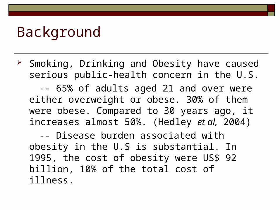
Smoking, Drinking and Obesity have caused serious public-health concern in the U.S.
-- 65% of adults aged 21 and over were either overweight or obese. 30% of them were obese. Compared to 30 years ago, it increases almost 50%. (Hedley et al, 2004)
-- Disease burden associated with obesity in the U.S is substantial. In 1995, the cost of obesity were US$ 92 billion, 10% of the total cost of illness.
In 2000, tobacco smoking caused more than 400,000 deaths. Smoking has been a leading preventable cause of mortality in the United States. Recently, anti-smoking has been an important policy in U.S.
Evidence from public health has shown that drinking may be associated with smoking behavior.
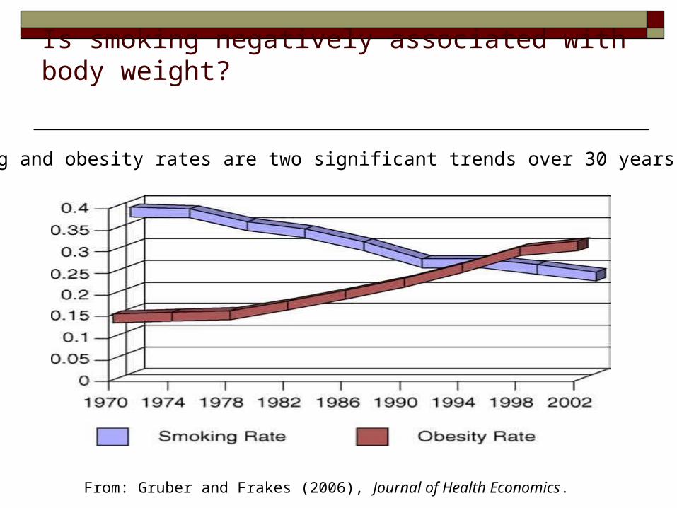
Is smoking negatively associated with body weight?
From: Gruber and Frakes (2006), Journal of Health Economics.
Smoking and obesity rates are two significant trends over 30 years in U.S

Literature Review
Study Data Method Conclusion
This Study CSFII 1994-1996 Quantile
Chen et al . (2007) CSFII 1994-1996 Censored Smoking has insignificant effect on BMI
Gruber and Frakes(2006)BRFSS 1984-2002 IV No evidence that smoking leads to weight gain
Ruidavets et al . (2002) France Survey OLS Positive of smoking and BMI
Chou et al. (2004) BRFSS 1984-2002 OLS Cigarette price (+); alcohol price (-) on BMI.
Lin et al. (2004) CSFII 1994-1996 OLS Smokers tend to be thinner than non-smokers
Wilson et al. (2004) St. Louis Survey Logit Smoking leads to low body weight
Jee et al. (2002) Korea Health Survey Logit Smoking leads to low body weight

What do we learn from previous studies?
Association between body weight and unhealthy decisions: The evidence whether the increased alcohol
consumption contributes to body weight is mixed. However, it may be important to distinct the effects of drinking beer and liquor.
Smoking tends to be negatively associated with body weight. However, the negative evidence has been re-investigated recently. (Chen et al, 2007. Gruber and Frakes 2006).

What may drive these inconclusive results?
Interrelationship between unhealthy decisions:
Smoking and drinking are highly correlated. Failing to control for one in estimation may lead to serious bias. (Kenkel and Wang 1999).
Conditional mean effect:
Most of the studies relied on the ordinary least squares (OLS). However, this method might not be sufficient in the context of obesity. (Kan and Tsai 2004).
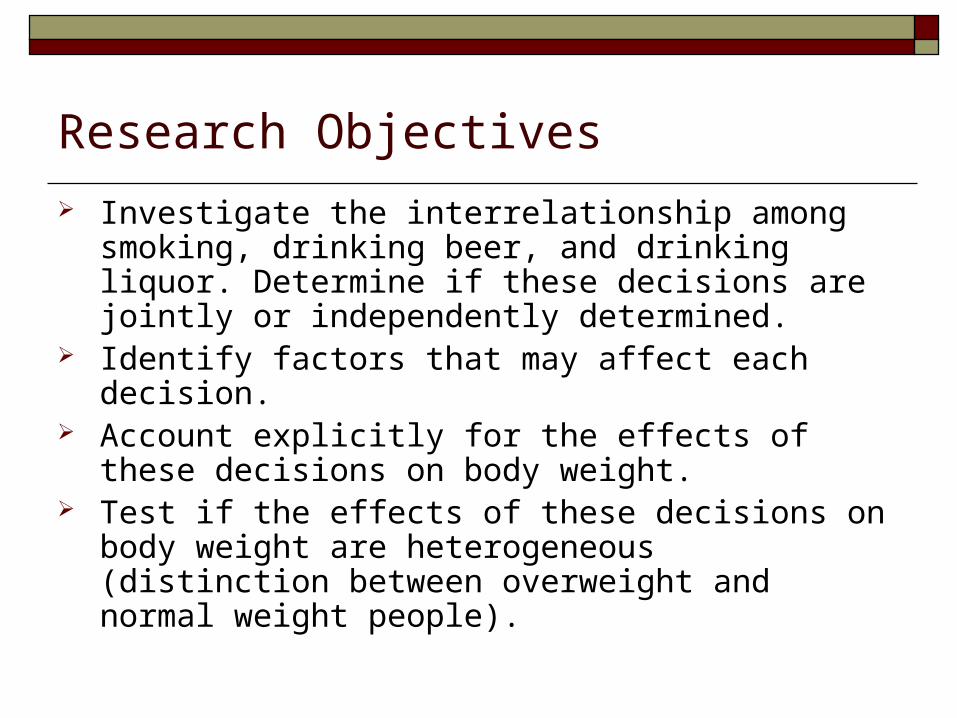
Research Objectives
Investigate the interrelationship among smoking, drinking beer, and drinking liquor. Determine if these decisions are jointly or independently determined.
Identify factors that may affect each decision. Account explicitly for the effects of these decisions
on body weight. Test if the effects of these decisions on body weight
are heterogeneous (distinction between overweight and normal weight people).

Data
Data from Continuing Survey of Food Intakes by Individuals (CSFII 1994-1996) is used. This data set is conducted by USDA.
We exclude individuals under 20 years-old. The final sample size includes 3,409 adult of this
survey. Body weight is measured as body mass index (BMI),
weight in kilograms divided by height in meters squared.

Distribution of BMI in our selected sample
Mean 26.5Std. Dev. 5.7Skewness 1.4Kurtosis 7.1
10% 20.420% 21.925% 22.530% 23.240% 24.4
45% 25.050% 25.660% 26.670% 28.375% 29.2
78% 30.080% 30.390% 33.7
Percentile
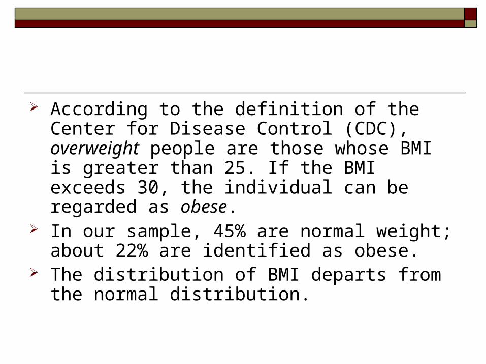
According to the definition of the Center for Disease Control (CDC), overweight people are those whose BMI is greater than 25. If the BMI exceeds 30, the individual can be regarded as obese.
In our sample, 45% are normal weight; about 22% are identified as obese.
The distribution of BMI departs from the normal distribution.
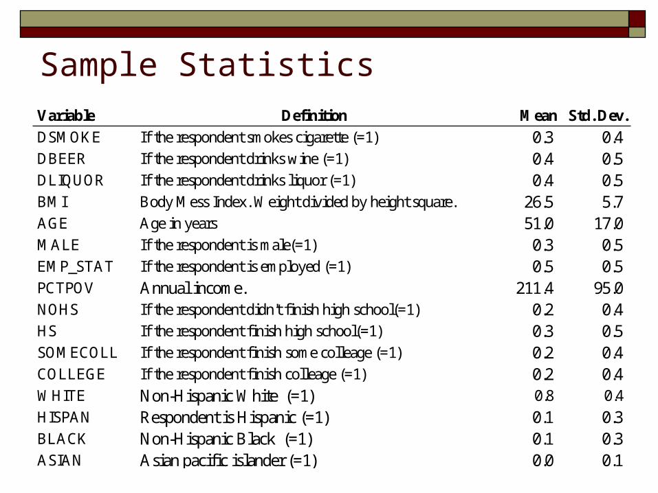
Sample StatisticsVariable Definition Mean Std. Dev.
DSMOKE If the respondent smokes cigarette (=1) 0.3 0.4DBEER If the respondent drinks wine (=1) 0.4 0.5DLIQUOR If the respondent drinks liquor (=1) 0.4 0.5BMI Body Mess Index. Weight divided by height square. 26.5 5.7AGE Age in years 51.0 17.0MALE If the respondent is male(=1) 0.3 0.5EMP_STAT If the respondent is employed (=1) 0.5 0.5PCTPOV Annual income. 211.4 95.0NOHS If the respondent didn't finish high school(=1) 0.2 0.4HS If the respondent finish high school(=1) 0.3 0.5SOMECOLL If the respondent finish some colleage (=1) 0.2 0.4COLLEGE If the respondent finish colleage (=1) 0.2 0.4WHITE Non-Hispanic White (=1) 0.8 0.4
HISPAN Respondent is Hispanic (=1) 0.1 0.3BLACK Non-Hispanic Black (=1) 0.1 0.3ASIAN Asian pacific islander (=1) 0.0 0.1
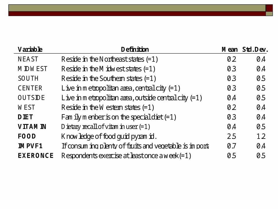
Variable Definition Mean Std. Dev.
NEAST Reside in the Northeast states (=1) 0.2 0.4MIDWEST Reside in the Midwest states (=1) 0.3 0.4SOUTH Reside in the Southern states (=1) 0.3 0.5CENTER Live in metropolitan area, central city (=1) 0.3 0.5OUTSIDE Live in metropolitan area, outside central city (=1) 0.4 0.5WEST Reside in the Western states (=1) 0.2 0.4DIET Family menber is on the special diet (=1) 0.3 0.4VITAMIN Dietary recall of vitamin user (=1) 0.4 0.5FOOD Knowledge of food guid pyramid. 2.5 1.2IMPVF1 If consuming plenty of fruits and vegetable is important (=1)0.7 0.4EXERONCE Respondents exercise at least once a week(=1) 0.5 0.5
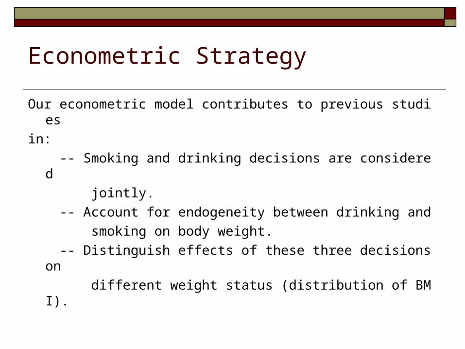
Econometric Strategy
Our econometric model contributes to previous studies
in:
-- Smoking and drinking decisions are considered
jointly.
-- Account for endogeneity between drinking and
smoking on body weight.
-- Distinguish effects of these three decisions on
different weight status (distribution of BMI).
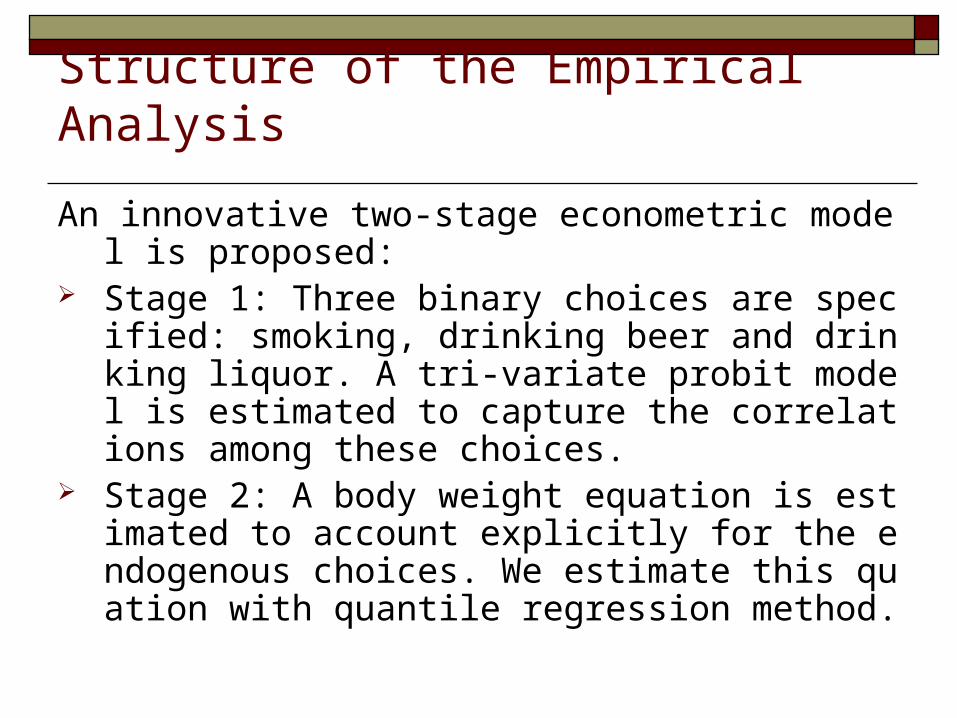
Structure of the Empirical Analysis
An innovative two-stage econometric model is proposed: Stage 1: Three binary choices are specified: smoking,
drinking beer and drinking liquor. A tri-variate probit model is estimated to capture the correlations among these choices.
Stage 2: A body weight equation is estimated to account explicitly for the endogenous choices. We estimate this quation with quantile regression method.

Stage 1: Modeling the joint decisions (trivariate probit model)
RHO (S,B)
RHO (S,W) RHO (W,B)
Smoking
Drinking Wine
Drinking Beer

Stage 1: (cont.)
1111 '* eXHI
2222 '* eXHI
3333 '* eXHI
Smoking Decision
Decision to drink beer
Decision to drink wine
)
1
1
1
;0,0,0(~),,(
3231
3221
3121
321
Neee

Estimate the discrete choice model (MLE)
The probability of regime (1,1,1):
Log likelihood function of the entire eight regimes:
],,,',','[loglog 2332133112213332221111
kkkkkkXHkXHkXHkLn
i
)',','Pr()1,1,1Pr( 33322211132111 XHeXHeXHeIIIP
),,,',','( 231312332211 XHXHXH
where k1=2I1-1, k2=2I2-1, k3=2I3-1
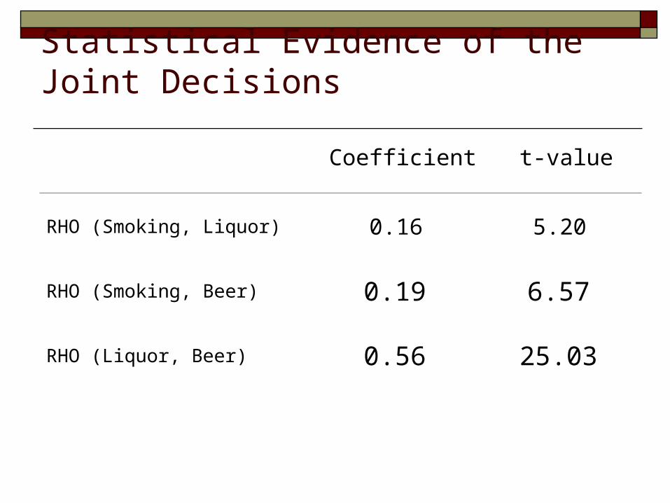
Statistical Evidence of the Joint Decisions
Coefficient t-value
RHO (Smoking, Liquor) 0.16 5.20
RHO (Smoking, Beer) 0.19 6.57
RHO (Liquor, Beer) 0.56 25.03

Correlations between smoking and drinking
Drinking beer and liquor is strongly associated (56%).
The decisions to smoke and to drink beer are significantly correlated (19%). In addition, the correlation between drinking liquor and smoking is 16%.
This is consistent with the evidence of public health in terms of the “gateway effect”.

Other Determinants of Smoking and Drinking
Variable Coef. t-value Coef. t-value Coef. t-value
FOOD -0.04 -1.96 0.01 0.54 0.03 1.52IMPVF1 -0.27 -4.90 -0.09 -1.58 -0.05 -0.91DIET -0.12 -2.04 -0.10 -1.91 -0.19 -3.58VITAMIN -0.13 -2.37 -0.03 -0.67 0.00 0.02EXERONCE -0.18 -3.45 -0.01 -0.23 0.16 3.42PCTPOV 0.00 -2.80 0.00 5.82 0.00 5.09AGE -0.01 -7.17 -0.01 -8.38 -0.02 -10.69MALE 0.13 2.48 0.23 4.57 0.80 15.50EMP_STAT 0.03 0.54 0.12 2.17 0.11 2.01NOHS1 0.59 6.76 -0.53 -6.30 -0.19 -2.37HS1 0.60 8.50 -0.28 -4.40 -0.16 -2.40SOMECOLL 0.39 5.06 -0.09 -1.29 -0.13 -1.90
Smoking Drinking Liquor Drinking Beer

Variable Coef. t-value Coef. t-value Coef. t-value
ASIAN -0.99 -3.24 -0.98 -4.01 -0.45 -2.17BLACK -0.06 -0.69 -0.10 -1.17 0.14 1.91HISPAN -0.30 -2.93 -0.43 -4.28 -0.06 -0.59OTHER 0.33 1.69 -0.19 -0.83 -0.05 -0.21WEST 0.22 2.67 -0.01 -0.17 0.10 1.33SOUTH 0.13 1.85 -0.43 -6.46 -0.16 -2.41MIDWEST 0.16 2.15 -0.10 -1.51 0.05 0.69CENTER 0.04 0.53 0.25 3.81 0.13 1.97OUTSIDE -0.03 -0.57 0.11 1.76 0.02 0.31
Smoking Drinking Liquor Drinking Beer

Empirical findings
Perception and knowledge of healthy food consumption decrease the likelihood to smoke.
Low education and income lead to high chance to smoke, but low chance to drink wine.
Male is more likely to smoke, and to drink beer. Job status increases the propensity to drink wine. Young generation has high probability to smoke. Other lifestyles also matter. If family members are
on diet, they are less likely to smoke, and to drink beer and liquor.

How much we believe in our model specification?-- Empirical results of statistical tests
Quantiles Test value#
Smoking 25% 10.14Drinking Liquor 50% 20.15Drinking Beer 75% 15.62
Quantiles Test-value##
Smoking 25% 2.73Drinking Liquor 50% 2.15Drinking Beer 75% 1.39* Ho: exogeneity
**Ho: additional varialbes are valid
# Critical value is F[3,3386]
## Critical value x 2 (0.95,3)=7.81
Overidentification Test**
Endogeneity Test*

Findings
If binary indicators are used, they are endogenous to the body weight. Therefore, there is a call for instruments (IV).
When instruments are used, statistical tests show that the added restrictions are not rejected. In other words, our selected instruments are not over-identified.

Stage 2: Body Weight Equation
The body weight equation is specified as:
To avoid endogeneity, predicted probabilities are
used as instruments for Ij. Quantile regression is
used to estimate this equation (Koenker and Bassett
1978).
eIdIdIdXBMI 332211 ***'
332211321 ***'),,,|( IdIdIdXIIIXBMIQ
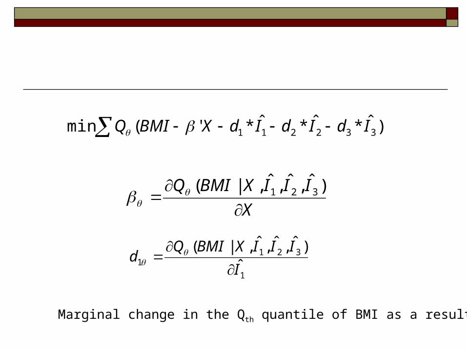
)ˆ*ˆ*ˆ*'(min 332211 IdIdIdXBMIQ
X
IIIXBMIQ
)ˆ,ˆ,ˆ,|( 321
1
3211 ˆ
)ˆ,ˆ,ˆ,|(
I
IIIXBMIQd
Marginal change in the Qth quantile of BMI as a result of change in X

Evidence of heterogeneous effects on BMI
Coef. t-value Coef. t-value Coef. t-value Coef. t-value
PSMOKE -4.8 -2.7 -1.4 -0.8 -2.7 -1.5 -4.7 -1.9PLIQUOR -8.7 -3.4 -3.5 -1.2 -7.0 -2.6 -10.8 -3.0PBEER 10.1 3.4 6.5 2.2 8.4 2.6 10.6 2.8
OLS 25% 50% 75%
F Test ** test p-value25% vs 50% 2.72 0.0125% vs 75% 21.43 0.0050% vs 75% 8.98 0.00

Effect of smoking on BMI distribution
-25
-20
-15
-10
-5
0
5
10
0.05 0.15 0.25 0.35 0.45 0.55 0.65 0.75 0.85 0.95
Percentiles
OLS
PSMOKE
PSMOKE_U
PSMOKE_L
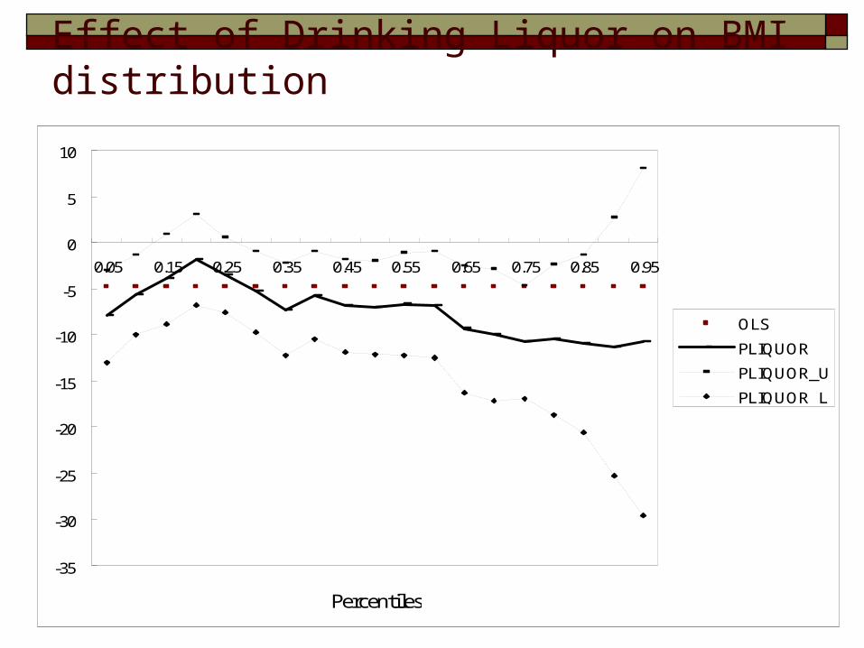
Effect of Drinking Liquor on BMI distribution
-35
-30
-25
-20
-15
-10
-5
0
5
10
0.05 0.15 0.25 0.35 0.45 0.55 0.65 0.75 0.85 0.95
Percentiles
OLS
PLIQUOR
PLIQUOR_U
PLIQUOR_L
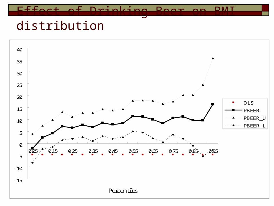
Effect of Drinking Beer on BMI distribution
-15
-10
-5
0
5
10
15
20
25
30
35
40
0.05 0.15 0.25 0.35 0.45 0.55 0.65 0.75 0.85 0.95
Percentiles
OLS
PBEER
PBEER_U
PBEER_L
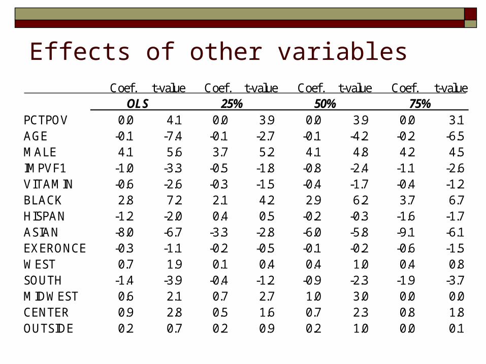
Effects of other variablesCoef. t-value Coef. t-value Coef. t-value Coef. t-value
PCTPOV 0.0 4.1 0.0 3.9 0.0 3.9 0.0 3.1AGE -0.1 -7.4 -0.1 -2.7 -0.1 -4.2 -0.2 -6.5MALE 4.1 5.6 3.7 5.2 4.1 4.8 4.2 4.5IMPVF1 -1.0 -3.3 -0.5 -1.8 -0.8 -2.4 -1.1 -2.6VITAMIN -0.6 -2.6 -0.3 -1.5 -0.4 -1.7 -0.4 -1.2BLACK 2.8 7.2 2.1 4.2 2.9 6.2 3.7 6.7HISPAN -1.2 -2.0 0.4 0.5 -0.2 -0.3 -1.6 -1.7ASIAN -8.0 -6.7 -3.3 -2.8 -6.0 -5.8 -9.1 -6.1EXERONCE -0.3 -1.1 -0.2 -0.5 -0.1 -0.2 -0.6 -1.5WEST 0.7 1.9 0.1 0.4 0.4 1.0 0.4 0.8SOUTH -1.4 -3.9 -0.4 -1.2 -0.9 -2.3 -1.9 -3.7MIDWEST 0.6 2.1 0.7 2.7 1.0 3.0 0.0 0.0CENTER 0.9 2.8 0.5 1.6 0.7 2.3 0.8 1.8OUTSIDE 0.2 0.7 0.2 0.9 0.2 1.0 0.0 0.1
OLS 25% 50% 75%
Empirical findings
A significant evidence supports the misspecification of using OLS. The effects are heterogeneous across the entire distribution of BMI.
Smoking tends to be negatively correlated with BMI. However, it is insignificant over the entire distribution of BMI.
Drinking beer tends to increase the body weight. However, this effect is not significant for obese people (above 85 percentile).

Drinking liquor is found negatively associated with body weight. In addition, the decreasing effect is significant for obese people (75 percentile).
Knowledge of healthy food consumption decreases the risk of being overweight.
Higher income leads to lower body weight. Race is also associated with body weight. Black
have heavy weight than others, on average; Asian are those with less weight.

Concluding and Policy Implications
The discussion of smoking, drinking and obesity should be interpreted with caution. We have shown:
-- strong correlations between smoking, drinking beer and drinking liquor.
-- heterogeneous effects of these decisions on BMI. The effect of smoking on body weight is found
insignificant. As such, anti-smoking may not be the critical factor driving the increasing trend of body weight over 30 years.
Drinking liquor is found negatively associated with body weight. Particularly, the effect is even stronger for normal weight people.
Drinking beer tends to increase body weight regardless of the weight status. Beer drinkers are those in a higher risk of being overweight.
Knowledge of healthy food consumption also have direct and indirect effects on body weight. A well-educated consumer has less likelihood of being overweight.


