179
User Manual
| Date post: | 12-Apr-2018 |
| Category: |
Documents |
| Upload: | teodora-cornea |
| View: | 260 times |
| Download: | 2 times |

7/21/2019 SOBEK - UserManual
http://slidepdf.com/reader/full/sobek-usermanual 1/179
User Manual
7/21/2019 SOBEK - UserManual
http://slidepdf.com/reader/full/sobek-usermanual 2/179
Table of Contents
User Manual___________________________________________________________________________________1
About Sobek 1Introduction.......................................................................................................................................................................1How is SOBEK organised?......................................... ............................ ............................. ............................ ................ 1When to use SOBEK and when not?...............................................................................................................................2The SOBEK manuals................................... ............................ ............................ ............................. ............................ ... 2The SOBEK user..............................................................................................................................................................3How to use this manual?..................................................................................................................................................3Hardware requirements....................................................................................................................................................3Product support..................................... ............................ ............................ ............................. ............................ .......... 3
Getting Started 4Working with SOBEK....................................................................................................................................................... 4Setting up of the model................................ ............................ ............................ ............................ ............................. ... 4Simulations.......................................................................................................................................................................6Analysis of results............................................................................................................................................................ 7Modelling with SOBEK-RE...............................................................................................................................................7
The Case Manager 12About the Case Manager................................... ............................ ............................ ............................ ........................ 12Projects and cases.........................................................................................................................................................12Project management options......................................................................................................................................... 13Working in a project........................................................................................................................................................ 14
Working in a project..................................... ............................. ............................ ............................ ......................... 14The Modelling Tasks..................................................................................................................................................16Colours.......................................................................................................................................................................16Activating a task.........................................................................................................................................................17Additional functions on task blocks............................................................................................................................17
Processes Library 17Processes Library Configuration Tool............................................................................................................................17
Processes Library Configuration Tool........................................................................................................................17The Selection of Active Substance Groups....................................... ............................. ............................ ............... 17
Selection of "State Variables" or "Substances" within a group..................................................................................18Selection of Water Quality Processes Affecting the State variables................................................ ......................... 19Specifying or Editing a Process........................................... ............................ ............................. ............................ . 20Extra Processes.........................................................................................................................................................22Saving the Configuration............................................................................................................................................22Processes Library Coefficient Editor..........................................................................................................................22
Sobek's User Interface 24Introduction on windows.................................................................................................................................................24Layout of windows..........................................................................................................................................................25Key shortcuts for buttons............................................................................................................................................... 25Buttons................................ ............................ ............................ ............................. ............................ .......................... 25Lists............................... ............................ ............................. ............................ ............................ ............................ .... 28Data fields...................................................................................................................................................................... 28Tables.............................................................................................................................................................................28Insensitive buttons and data fields.................................................................................................................................29Important windows......................................................................................................................................................... 29Formats............................... ............................ ............................ ............................. ............................ .......................... 29Default values.................................................................................................................................................................30Descriptions of windows.................................................................................................................................................30
Sobek Model Window 30Sobek-model window................................... ............................ ............................ ............................. ............................ . 30Model Attributes............................................................................................................................................................. 31Layers.............................................................................................................................................................................32
ii
7/21/2019 SOBEK - UserManual
http://slidepdf.com/reader/full/sobek-usermanual 3/179
Table of Contents
Topography........................................ ............................. ............................ ............................ ............................ ........... 33Topography....................................... ............................ ............................ ............................. ............................ ........ 33Nodes.........................................................................................................................................................................34Join of nodes..............................................................................................................................................................34Branches.......................................... ............................ ............................ ............................. ............................ ......... 35Splitting of a branch..................................... ............................. ............................ ............................ ......................... 37
Cross-Sections............................................... ............................. ............................ ............................ ........................... 38Cross-Sections...........................................................................................................................................................38Cross-Section Description......................................................................................................................................... 38Cross-sections Placement....................................... ............................. ............................ ............................ ............. 41
Structures....................................... ............................ ............................ ............................. ............................ ............... 42Structures...................................................................................................................................................................42Structure description...................................... ............................ ............................ ............................. ....................... 42Weir Description.........................................................................................................................................................43Advanced Weir Description........................................................................................................................................43General Structure Description................................................................................................................................... 44Pump Description.......................................................................................................................................................45Database Structure Description.................................................................................................................................45Structure Placement.................................................................................................................................................. 48
Controllers...................................... ............................ ............................ ............................. ............................ ............... 49Controllers..................................................................................................................................................................49Triggers...................................... ............................ ............................ ............................. ............................ ............... 53
Friction............................................................................................................................................................................54Friction....................................................................................................................................................................... 54Bed friction WF...........................................................................................................................................................54Wind friction WF.........................................................................................................................................................55Extra resistance......................................................................................................................................................... 55
Conditions...................................................................................................................................................................... 55Conditions................................... ............................ ............................ ............................. ............................ .............. 55Boundary conditions water flow.................................. ............................ ............................ ............................. .......... 56Discharge at branches............................................ ............................. ............................ ............................ .............. 56Conditions salt............................................................................................................................................................57Conditions sediment/morphology.............................................................................................................................. 58Conditions water quality.............................................................................................................................................59
Water quality at boundaries........................................... ............................ ............................. ............................ ....... 60Water quality flow at branches (!)................................... ............................ ............................. ............................ ...... 60Water quality at branches............................................. ............................ ............................ ............................. ........ 60Water quality conditions import options.....................................................................................................................60
Initial Conditions.................................... ............................ ............................ ............................. ............................ ........ 61Initial conditions.......................................................................................................................................................... 61Water flow.............................. ............................ ............................. ............................ ............................ ................... 61Salt............................. ............................. ............................ ............................ ............................ ............................. .. 61Morphodynamics........................................................................................................................................................61Water quality................................ ............................ ............................. ............................ ............................ ............. 62
Meteo Data.....................................................................................................................................................................62Meteo data............................. ............................ ............................. ............................ ............................ ................... 62
Dispersion...................................................................................................................................................................... 63Dispersion........................................ ............................ ............................ ............................ ............................. ......... 63
Grid.................................................................................................................................................................................64Grid definition............................... ............................. ............................ ............................ ............................ ............. 64Grid points..................................................................................................................................................................64WQ-Segments............................................................................................................................................................65
Runtime Data................................................................................................................................................................. 66Introduction Run time data.........................................................................................................................................66Time parameters........................................................................................................................................................67Numerical parameters................................................................................................................................................68Output f(x)................................... ............................ ............................ ............................. ............................ .............. 71Output f(t)............................... ............................. ............................ ............................ ............................ ................... 73
iii
7/21/2019 SOBEK - UserManual
http://slidepdf.com/reader/full/sobek-usermanual 4/179
User Manual
Transport Formula..........................................................................................................................................................74Transport formula.......................................................................................................................................................74
Groundwater...................................................................................................................................................................74Groundwater.............................................................................................................................................................. 74
Making calculations 75Making calculations........................................................................................................................................................75
Cutting and Combining of Schematisations 75Introduction cutting and combining schematisations......................................... ............................ ............................ .... 75How to cut a schematisation.................................... ............................ ............................ ............................ .................. 75How to combine two schematisations............................................................................................................................76
Application of Sobek 76General...........................................................................................................................................................................76River training.............................. ............................ ............................. ............................ ............................ ................... 77Dredging optimization.................................................................................................................................................... 77Water quality.................................................................................................................................................................. 77River bend cut-offs................................. ............................ ............................ ............................. ............................ ....... 77Water flow...................................................................................................................................................................... 78Regime changes............................................................................................................................................................ 78Flood risk........................................................................................................................................................................78Low water.................................. ............................ ............................. ............................ ............................ .................... 78Major limitations............................................................................................................................................................. 79
One-dimensional........................................................................................................................................................79Horizontal water surface...................................... ............................ ............................ ............................ .................. 79Sub-critical flow..........................................................................................................................................................79
Tutorial 79General...........................................................................................................................................................................79Setting up of the model................................ ............................ ............................ ............................ ............................. . 80Topography........................................ ............................. ............................ ............................ ............................ ........... 82Cross sections................................................................................................................................................................85Structures....................................... ............................ ............................ ............................. ............................ ............... 90Friction............................................................................................................................................................................92Conditions...................................................................................................................................................................... 93Initial conditions..............................................................................................................................................................97Grid definition............................. ............................ ............................. ............................ ............................ ................... 97
Run time data.................................. ............................ ............................. ............................ ............................ .............. 98 Appendix A (Installation & Authorization) 100
Installation on PC...................................... ............................. ............................ ............................ ............................ .. 100Directory Structure....................................................................................................................................................... 100Startup directory related to 'Import/export files'........................................................................................................... 100Software authorization................................................................................................................................................. 100FLEXlm on a Windows computer.................................................................................................................................100FLEXlm daemon on a Windows server........................................................................................................................101FLEXlm License Manager as a service....................................................................................................................... 101LMTools Utility..............................................................................................................................................................103
Appendix B (Messages) 103SOBEK Messages........................................................................................................................................................ 103Messages User Interface.............................. ............................ ............................ ............................. .......................... 103
Messages User Interface 0 - 999.............................................................................................................................103Messages User Interface 1000 - 1999..................................................................................................................... 104Messages User Interface 2000 - 2999..................................................................................................................... 105Messages User Interface 3000 - 3999..................................................................................................................... 107Messages User Interface 4000 - 4999..................................................................................................................... 108Messages User Interface 5000 - 5999..................................................................................................................... 108Messages User Interface 6000 - 6999..................................................................................................................... 108Messages User Interface 7000 - 7999..................................................................................................................... 109Messages User Interface 8000 - 8999..................................................................................................................... 109Messages User Interface 9000 - 9999..................................................................................................................... 109Messages User Interface 10000 - 10999................................................................................................................ 109
iv
7/21/2019 SOBEK - UserManual
http://slidepdf.com/reader/full/sobek-usermanual 5/179
Table of Contents
Messages User Interface 11000 - 11999................................................................................................................ 109Messages User Interface 12000 - 12999................................................................................................................ 110Messages User Interface 13000 - 13999................................................................................................................ 111Messages User Interface 14000 - 14999................................................................................................................ 112Messages User Interface 15000 - 15999................................................................................................................ 112Messages User Interface 16000 - 16999................................................................................................................ 112Messages User Interface 17000 - 17999................................................................................................................ 112Messages User Interface 18000 - 18999................................................................................................................ 113Messages User Interface 19000 - 19999................................................................................................................ 123Messages User Interface 20000 - 20999................................................................................................................ 124Messages User Interface 21000 - 21999................................................................................................................ 124Messages User Interface 22000 - 22999................................................................................................................ 125Messages User Interface 23000 - 23999................................................................................................................ 125Messages User Interface 24000 - 24999................................................................................................................ 125Messages User Interface 25000 - 25999................................................................................................................ 125
Other messages............................................. ............................. ............................ ............................ ......................... 126Messages computational core.................................... ............................ ............................ ............................. ........ 126Main module messages....................................... ............................ ............................ ............................. ............... 126Flow module messages.......................................... ............................ ............................. ............................ ............ 128Salt intrusion module messages..............................................................................................................................131Sediment transport module messages............................................ ............................ ............................ ................ 132Morphology module messages................................................................................................................................133Water quality interface module messages...............................................................................................................134Graded sediment messages....................................................................................................................................135
Appendix C (Import / Export) 136Import/Export of files.................................. ............................. ............................ ............................ ............................ . 136Reading tables from ASCII file............................. ............................. ............................ ............................ ................... 137Tables with header from ASCII file.............................................................................................................................. 137Importing cross section.................................... ............................. ............................ ............................ ....................... 138Importing Water Quality Conditions.................................... ............................ ............................. ............................ .... 140
Appendix D (Conversion) 141Step A: Preparing Conversion of Models.....................................................................................................................141Step B: Perform Conversion of Models........................................................................................................................142Step C: Importing your converted model into SOBEK 2..............................................................................................142
Appendix E (Restart) 142Restart of model calculation.........................................................................................................................................142
Appendix F (Introduction to water quality modelling with Sobek) 143Introduction...................................................................................................................................................................143
General.................................................................................................................................................................... 143What is a water quality model?................................................................................................................................144
Water quality modelling with Sobek......................................... ............................ ............................. ........................... 144Mass balance for pollutants.................................. ............................ ............................ ............................. .............. 144Integrated modelling of Channel Flow and Water Quality............................................... ............................ ............ 145Overview of input items............................................................................................................................................145
About schematisations.......................................... ............................. ............................ ............................ .................. 146Basic schematisation elements............................................................................................................................... 146Control volumes...................................... ............................ ............................ ............................ ............................. 146
Water balance...................................... ............................ ............................ ............................ ............................. ....... 146Water balance for control volumes....................................... ............................ ............................. .......................... 146Water balance check............................................................................................................................................... 147
Transport of pollutants in the channel flow network.....................................................................................................147Fraction computations..............................................................................................................................................147Transport over interfaces between 2 segments...................................................................................................... 148Transport of pollutants over open boundaries..................................... ............................ ............................ ............ 150Transport of pollutants from lateral discharges....................................................................................................... 150Evaporation....................................... ............................ ............................ ............................. ............................ ...... 151Transport of pollutants around structures................................................................................................................151
Modelling the substance specific source term.............................. ............................ ............................ ....................... 151
v
7/21/2019 SOBEK - UserManual
http://slidepdf.com/reader/full/sobek-usermanual 6/179
User Manual
The Delwaq Processes Library................................................................................................................................151Using the Delwaq Processes Library.......................................................................................................................152Numerical aspects................................................................................................................................................... 152
Appendix G (Delwaq Processes Library) 153Preface..................................... ............................ ............................ ............................. ............................ ................... 153Introduction of Processes Library and Editor...............................................................................................................154Setup of Processes Library and Editor........................................................................................................................ 154
Water Quality Modelling...........................................................................................................................................154Processes Library....................................... ............................ ............................. ............................ ........................ 155Processes Editor......................................................................................................................................................156
Application of Processes Library and Editor................................ ............................ ............................ ........................ 156Application of Processes Library and Editor............................................................................................................156Taihu Basin Oxygen Model......................................................................................................................................157Friesland Province Eutrophication Model................................ ............................ ............................ ........................ 157Dutch Coastal Waters Eutrophication Model...........................................................................................................158Scheldt Estuary: Oxygen, Eutrophication and Heavy Metals Model............................................ ........................... 159
Appendix H (Structure Control options in Sobek-RE) 160Structure Control Options incorporated in SOBEK River............................................................................................ 160General.........................................................................................................................................................................160Controlling Procedure Applied in SOBEK......................................... ............................ ............................ ................... 161Overview of Controllers Available in SOBEK...............................................................................................................162Controlles available in Sobek.......................................................................................................................................162
Time controller......................................................................................................................................................... 162Relative from Value Controller.................................................................................................................................164Hydraulic controller.................................. ............................ ............................ ............................ ............................ 165Interval controller..................................................................................................................................................... 166PID Controller...........................................................................................................................................................168
Triggers in Sobek...................................... ............................. ............................ ............................ ............................ .. 170Trigger Procedure Applied in SOBEK......................................................................................................................170
Index_______________________________________________________________________________________171
vi

7/21/2019 SOBEK - UserManual
http://slidepdf.com/reader/full/sobek-usermanual 7/179
User Manual
About Sobek
Introduction
SOBEK is the name of a highly sophisticated software package, which in concise technical terms is a one-dimensionalopen-channel dynamic numerical modelling system, equipped with the user shell and which is capable of solving theequations that describe unsteady water flow, salt intrusion, sediment transport, morphology and water quality.
In less technical terms SOBEK can be described as a flexible, powerful and reliable tool to simulate and solve problems inriver management, flood protection, design of canals, irrigation systems, water quality, navigation and dredging. A veryuser-friendly interface helps you schematise the problem and organise the required data into such a form that they can behandled by SOBEK's computational core. The interface also helps you in effective analysing and reporting of simulationresults. The user interface is operated through the keyboard and the mouse. The interface is organised in such a way,that you will have to do a minimum amount of typing and always get only those questions and selection options on thescreen that are relevant for the phenomena you wish to take into account. As an example: if the problem does not involvesediment transport, you tell SOBEK so at the start of the model preparation and after that the program won't refer to itanother time.
SOBEK was developed by WL | Delft Hydraulics in full partnership with the Institute for Inland Water Management andWaste Water Treatment (RIZA) of the Netherlands government. It is one of the core modelling systems of these twopartners, who guarantee continuing support and development of SOBEK.
And finally: SOBEK is named after the ancient Egyptian crocodile river god. Crocodiles were believed to have predictivepowers, as they were laying their eggs just above the level of the next Nile flood. We do not require you to have a likewisebelief in SOBEK. It has been thoroughly tested and what can be comforting to you: there are detailed validationdocuments that prove SOBEK's capabilities (available on request).
How is SOBEK organised?
SOBEK is capable of handling one-dimensional problems in open channel networks. Apart from steady or unsteady water flow, these problems can touch various other processes, like salt intrusion, sediment, morphology and water quality. Aseach type of problem may require its own solving methods, based on underlying theories and assumptions, SOBEKconsists of five modules. Each is related to one group of physical processes. Together they work as a fully integratedsoftware package. During the input phase you will make SOBEK aware of a specific problem and the program willautomatically select the related module. By properly defining the problem right from the start SOBEK will not bother youwith input screens that are not relevant to the application you will be building.
The modules of SOBEK-RE are, with their two-letter code used in the documentation:
• Water Flow - WF
• Salt Intrusion - SA
• Sediment Transport - ST
• Morphology - MO
• Water Quality - WQ
• Graded sediment - GS (Not Standard, there is a separate manual for Graded Sediment)
• Mozart - MZ (Not standard, for this water distribution model there is a separate manual)
• Groundwater Exchange - GW (Buffering of water in river banks)
Your selection of modules for a model can be changed in a later stage. SOBEK contains facilities for a correct processingof such a change. However, we recommend to make a correct selection of modules right at the start of making a newmodel, as including a certain process does not imply that you need to prepare all input data related to that process.
Apart from this problem-oriented approach SOBEK makes a distinction between the geophysical character of the network:
1
7/21/2019 SOBEK - UserManual
http://slidepdf.com/reader/full/sobek-usermanual 8/179
User Manual
• River
• Estuary
This distinction has more to do with the location of the problem than with the phenomena involved in the problem. If your system to be modelled is inland and far from tidal influence you select the "river" option. SOBEK will not bother you thenwith on-screen queries related to tides and to morphological matters that are typical for tidal (estuary) areas.
When to use SOBEK and when not?
As outlined earlier the modules of SOBEK cover a wide range of physical processes.
Typical applications of one or more of the available modules are:
• Flood protection studies
• Design of canal systems (e.g. for irrigation)
• Morphology related to dredging
• Salt intrusion in lower reaches of rivers
• River regulation
• Water quality studies in river basins and canal systems
• Sedimentation problems
SOBEK is a one-dimensional modelling system. This implies that SOBEK works with cross-sectional average values of parameters and variables. Some facilities to simulate two-dimensional effects in a rough way are available (likefloodplains in the cross-section, distinction between water quality processes in main channel and floodplain, and a methodfor quasi two-dimensional river morphology), but basically SOBEK cannot deal with questions and problems requiringdetailed insight into the two- or even three-dimensional flow field. For those problems other models are available(DELFT3D for two and three-dimensional problems).
Practice has shown that in cases when the flow system has a typical gully character, the basically two-dimensionalcharacter of the model area can be modelled quite acceptably with SOBEK's one-dimensional approach.
The maximum allowable size of your SOBEK model depends mainly on the memory capacity of the hardware. All bulkdata is stored dynamically meaning that it is impossible to say that a model on a 16Mb PC can have so many branchesand nodes. In practice, though, you will find that models with a hundred or even more branches will cause few problemson a PC with 16 Mb.
The SOBEK manuals
The SOBEK manual comes in two volumes:
• User ManualThis volume is in front of you. It provides ample information on the use of SOBEK: its installation, itsoperation via the user interface (preparation of input, simulation, processing of simulation results) andideas on how to catch your particular problem in a SOBEK application.
• Technical Reference Manual (TRM)This volume gives for each module an alphabetical list of keywords, with a brief explanation on itsmeaning in SOBEK and, when relevant, some background information and related formulas. The water quality part is not organised in keywords but has a process-oriented setup.
These manuals are also accessible on screen with the Help Menu Item and Help Key «F1».
2

7/21/2019 SOBEK - UserManual
http://slidepdf.com/reader/full/sobek-usermanual 9/179
User Manual
The SOBEK user
A prerequisite for a successful use of SOBEK is that the user has a basic knowledge of the phenomena covered by thevarious modules of SOBEK that the user wants to apply (water flow, sediment transport, density currents, water qualityand morphology). Although SOBEK has been made easy to handle and fairly "foolproof", it should always be applied witha fair insight into the problems and processes involved, and also keeping in mind whether the one-dimensional approachis acceptable. Despite much internal checking of the input, it is still possible that SOBEK accepts data beyond theapplication range for which it was prepared and will consequently generate calculation results that should be viewed withsuspicion. SOBEK will try to warn you as much as possible for doubtful elements in your input and data, but in the end thenotion " Garbage in, (more) garbage out " also holds for SOBEK!
Training in the use of SOBEK can be given by SOBEK suppliers, but we have tried to make the program so user-friendlythat it can be learnt almost intuitively.
How to use this manual?
To get the full benefit of SOBEK's capabilities in your applications you should spend ample time in studying this manualand running the tutorial. Before you start at the keyboard you should read Chapter 2 "Getting started", which explains thebasics of SOBEK: what are its elemental "building blocks" to make a network, how can structures be modelled, whatprocesses can you simulate in your application, what pictures of results can you get on your screen, and so on. Next youcan start SOBEK and work out a simple example to get a first impression on the look and feel of SOBEK's interface,through which all your communication with the computer takes place.
Depending on your earlier experience with computer models, in particular with predecessors of SOBEK, you can then firstrun the tutorial described in Chapter 5 or begin building a simple application yourself, and get further acquainted with theoperation of the user interface, with support of help key « F1 », the text of Chapter 3 and the Technical Reference Manual.
Type style conventions
In this manual the following conventions are used in type style:
Type style Used for
«Button» Buttons (on the screen or on the keyboard) that perform the indicated action or give access to a correspondingwindow. The text can be located on the button itself or next to the button.
"Window" Name of a window, shown in the name bar. Also used for sub windows, indicating a group of buttons and/or data fields.
'Text ' Text near data fields or item in a list.
Italic WF Parameters, formulas and terms that are a keyword in the Technical Reference Manual. The superscriptindicates the section. Usually it is placed only there where the term is printed for the firsttime.
The purpose of buttons, windows and data fields will become clear to you in the texts dealing with the interface.
Hardware requirements
SOBEK runs on personal computers under Microsoft Windows (2000, XP and Vista). The minimum requirement is aPentium processor and 512 Mb of internal memory. SOBEK needs also 20GB of free disk space to install theexecutables. Depending on the size of your models you need more disk space. The screen resolution should be at least800x600, and you have to use ‘small fonts’.
SOBEK can only run if a special software key has been installed. In this way unauthorised use of SOBEK is prevented.
Product support
If you have a question about SOBEK for which you cannot find the answer in the manual, you can contact SOBEK Supportat Deltares.
You should have the following information ready:
the version number of SOBEK (see headline of project or case manager);
3
7/21/2019 SOBEK - UserManual
http://slidepdf.com/reader/full/sobek-usermanual 10/179
User Manual
the type of hardware you are using, including network hardware if applicable;
the operating system you are using;
the exact wording of any message that appeared on your screen (write it down);
a description of what happened and what you were doing when the problem occurred;
a description of how you tried to solve the problem;
whether you are able to reproduce the problem by repeating what you did when the problem occurred?
You can contact SOBEK Support in the following ways:
Fax: +31 88 335 81 11
Phone: +31 88 335 85 00
E-mail: [email protected]
Getting Started
Working with SOBEK
We suppose that SOBEK has been installed on your computer system. Information how to install is described in Appendix Aof this manual. This Chapter explains the basics of SOBEK : what are its elemental "building blocks" to make a network, howcan structures be modelled, what processes can you simulate in your application, what pictures of results can you get onyour screen, and so on. After you start SOBEK you can go through a simple example to get a first impression on the lookand feel of SOBEK 's interface.
Chapter 1 gave you an overview of SOBEK 's potential field of applications. When you apply SOBEK for the solution of aproblem, you will usually work along the following lines. Your actions will fall into three main groups:
• Set up of the model
• Simulation
• Analysis of results
Setting up of the model
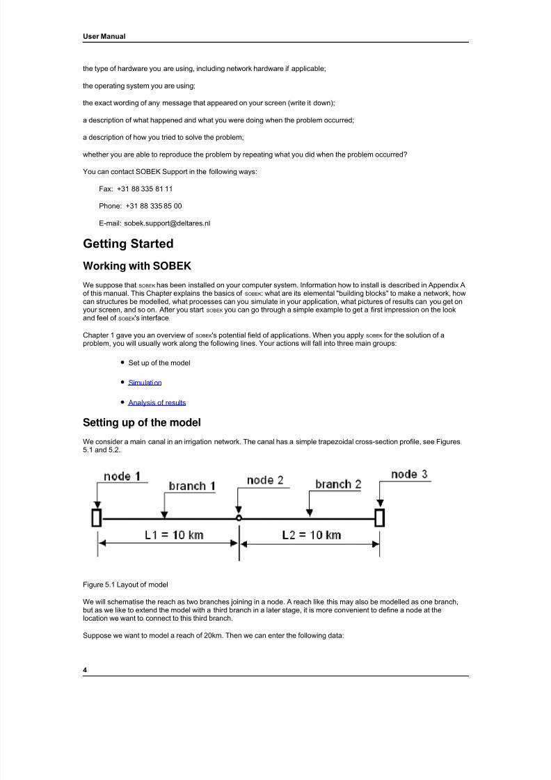
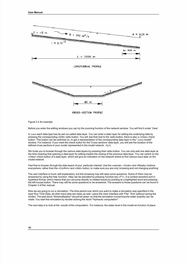
We consider a main canal in an irrigation network. The canal has a simple trapezoidal cross-section profile, see Figures5.1 and 5.2.
Figure 5.1 Layout of model
We will schematise the reach as two branches joining in a node. A reach like this may also be modelled as one branch,but as we like to extend the model with a third branch in a later stage, it is more convenient to define a node at thelocation we want to connect to this third branch.
Suppose we want to model a reach of 20km. Then we can enter the following data:
4
7/21/2019 SOBEK - UserManual
http://slidepdf.com/reader/full/sobek-usermanual 11/179
User Manual
Length of branch 1: 10000 m
Length of branch 2: 10000 m
Bed level slope: 2 10 -4
A positive slope means lower bed level in positive x-direction.
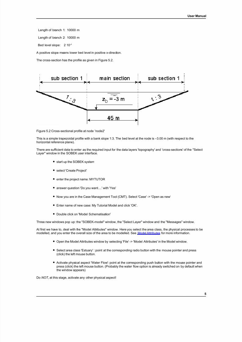
The cross-section has the profile as given in Figure 5.2.
Figure 5.2 Cross-sectional profile at node 'node2'
This is a simple trapezoidal profile with a bank slope 1:3. The bed level at the node is –3.00 m (with respect to thehorizontal reference plane).
There are sufficient data to enter as the required input for the data layers 'topography' and 'cross-sections' of the "SelectLayer" window in the SOBEK user interface.
• start up the SOBEK system
• select 'Create Project'
• enter the project name: MYTUTOR
• answer question 'Do you want....' with 'Yes'
• Now you are in the Case Management Tool (CMT). Select 'Case' -> 'Open as new'
• Enter name of new case: My Tutorial Model and click 'OK'.
• Double click on 'Model Schematisation'
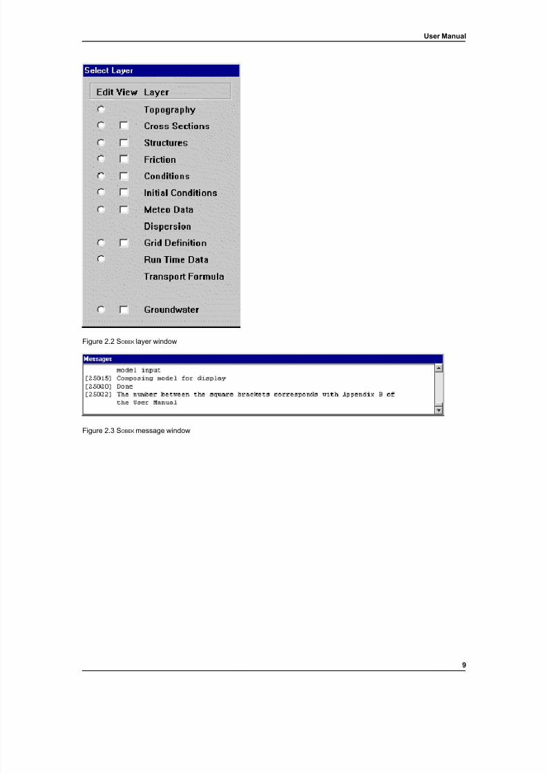
Three new windows pop up: the "SOBEK-model" window, the "Select Layer" window and the "Messages" window.
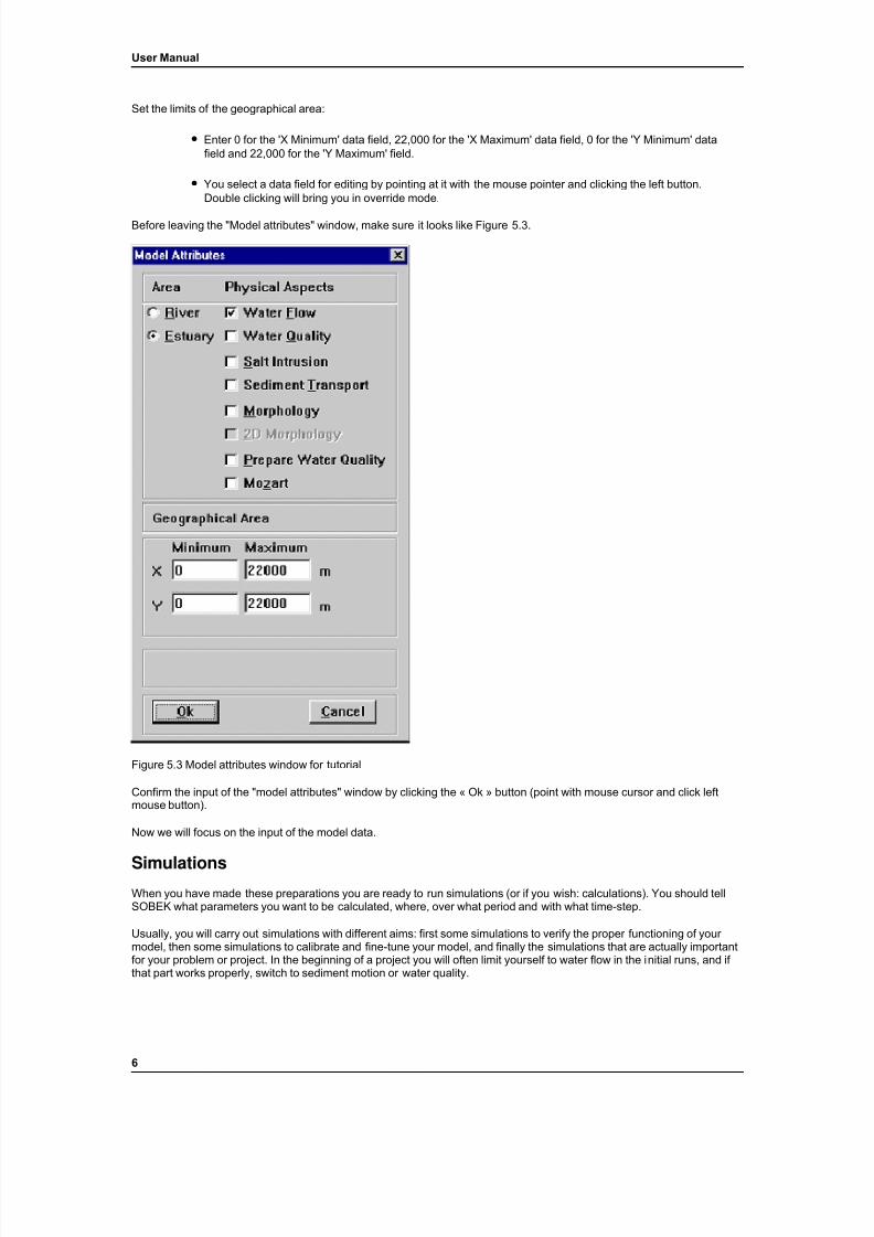
At first we have to, deal with the "Model Attributes" window. Here you select the area class, the physical processes to bemodelled, and you enter the overall size of the area to be modelled. See Model Attributes for more information.
• Open the Model Attributes window by selecting 'File' -> 'Model Attributes' in the Model window.
• Select area class 'Estuary' : point at the corresponding radio button with the mouse pointer and press(click) the left mouse button.
• Activate physical aspect 'Water Flow': point at the corresponding push button with the mouse pointer andpress (click) the left mouse button. (Probably the water flow option is already switched on by default whenthe window appears)
Do NOT , at this stage, activate any other physical aspect!
5
7/21/2019 SOBEK - UserManual
http://slidepdf.com/reader/full/sobek-usermanual 12/179
User Manual
Set the limits of the geographical area:
• Enter 0 for the 'X Minimum' data field, 22,000 for the 'X Maximum' data field, 0 for the 'Y Minimum' datafield and 22,000 for the 'Y Maximum' field.
• You select a data field for editing by pointing at it with the mouse pointer and clicking the left button.Double clicking will bring you in override mode.
Before leaving the "Model attributes" window, make sure it looks like Figure 5.3.
Figure 5.3 Model attributes window for tutorial
Confirm the input of the "model attributes" window by clicking the « Ok » button (point with mouse cursor and click leftmouse button).
Now we will focus on the input of the model data.
SimulationsWhen you have made these preparations you are ready to run simulations (or if you wish: calculations). You should tellSOBEK what parameters you want to be calculated, where, over what period and with what time-step.
Usually, you will carry out simulations with different aims: first some simulations to verify the proper functioning of your model, then some simulations to calibrate and fine-tune your model, and finally the simulations that are actually importantfor your problem or project. In the beginning of a project you will often limit yourself to water flow in the initial runs, and if that part works properly, switch to sediment motion or water quality.
6

7/21/2019 SOBEK - UserManual
http://slidepdf.com/reader/full/sobek-usermanual 13/179
User Manual
Analysis of results
After you have made a simulation you may wish to analyse the results. SOBEK can post process the computed results,which are written during the simulation to (binary) files. Graphs that are presented on screen and can easily be printed for further analysis and reporting. The postprocessor can also produce ASCII-files that can be read easily and further manipulated by other software like graphical presentation programs, spreadsheets, etc.
Modelling with SOBEK-RE After you have entered the project 'Tutorial' and opened the case ‘Example’, in the CMT, that comes with SOBEK , you startfurther working with that case by activating the task 'Schematisation'. Now three windows become visible:
• A window with the very basic network of the model .
• A layer window to access the layers of the model.
• A message window.
In the next section, you are invited to play around with the example model which is already open and ready for editing.
The example case (Figure 2.4 and 2.5) is extremely simple; it contains one branch only, but it has several optionsswitched on and incorporated.
Therefore it is very suitable to get a first impression of the edit function and meaning of data in SOBEK .
7

7/21/2019 SOBEK - UserManual
http://slidepdf.com/reader/full/sobek-usermanual 14/179
User Manual
Figure 2.1 S OBEK network window
8
7/21/2019 SOBEK - UserManual
http://slidepdf.com/reader/full/sobek-usermanual 15/179
User Manual
Figure 2.2 S OBEK layer window
Figure 2.3 S OBEK message window
9
7/21/2019 SOBEK - UserManual
http://slidepdf.com/reader/full/sobek-usermanual 16/179
User Manual
Figure 2.4 An example
Before you enter the editing windows you can try the zooming function of the network window. You will find it under ‘View’.
In SOBEK each data type has its own so-called data layer. You can enter a data layer for editing the underlying data bypressing the corresponding «Edit» radio button. You will see that next to the radio button, there is also a «View» checkbutton. This button can be switched on, to get a representation of the corresponding data layer in the " SOBEK -model"window. For instance: if you mark the check button for the 'Cross sections' data layer, you will see the location of thedefined cross sections in your model represented in the model network : try it.
We invite you to browse through the various data layers by pressing their radio button. You can only edit one data layer atthe time meaning that opening a data layer for editing implies the closing of the previous data layer. You can switch on the«View» check button of a data layer, which will give an indication on the network where to find various input data on themodel network.
Feel free to browse through the data layers of your particular interest. Use the «cancel», «Undo» and «Ready» buttonseverywhere, rather than the «Confirm» and «Add» button, to make sure you are only browsing and not changing anything.
The user interface is much self-explanatory, but this browsing may still raise some questions. Some of them may beanswered by using the help function. Help can be activated by pressing function key «F1». It is context-sensitive and inhypertext format, which means that you can jump directly to related issues by pointing at a highlighted word and pressingthe left mouse button. There may still be some questions to be answered. The answers to those questions can be found in
Chapter 3 of this manual.
Now we are going to run a simulation. The time period over which you want to make a simulation was specified in thelayer Run Time Data; all other input data are ready as well. Leave the User Interface with 'File', 'Exit' (without saving themodel). The task block "Schematisation" should be green so that the simulation concerning the water quantity can bemade. You start this simulation by double-clicking the block "Hydraulic computation".
The next step is to look at the results of the computation . For instance, the water level in the model as function of place.
10
7/21/2019 SOBEK - UserManual
http://slidepdf.com/reader/full/sobek-usermanual 17/179
User Manual
Before you start a simulation you define which parameters have to be calculated, at what places and with what timeinterval. After the completion of the simulation you can start the analysis of the computation results by clicking one of thetask blocks "Results in Charts". As you made only a hydraulic computation you select the block linked to "Hydrauliccomputation".
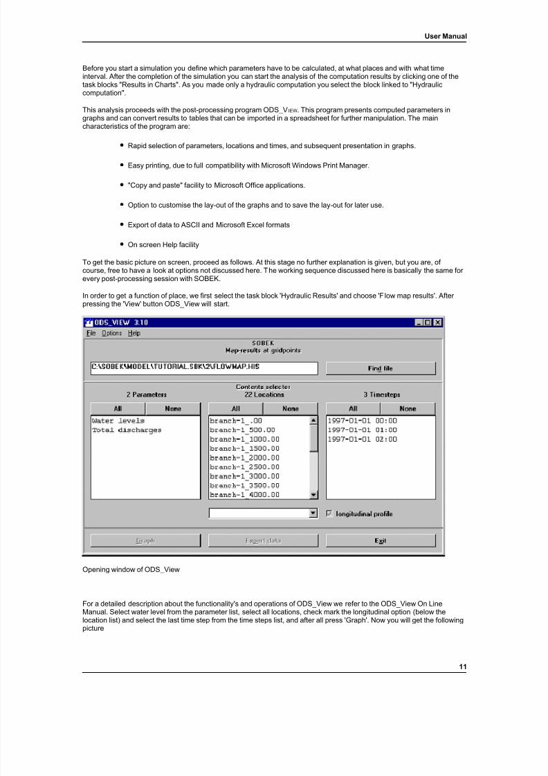
This analysis proceeds with the post-processing program ODS_V IEW. This program presents computed parameters ingraphs and can convert results to tables that can be imported in a spreadsheet for further manipulation. The maincharacteristics of the program are:
• Rapid selection of parameters, locations and times, and subsequent presentation in graphs.
• Easy printing, due to full compatibility with Microsoft Windows Print Manager.
• "Copy and paste" facility to Microsoft Office applications.
• Option to customise the lay-out of the graphs and to save the lay-out for later use.
• Export of data to ASCII and Microsoft Excel formats
• On screen Help facility
To get the basic picture on screen, proceed as follows. At this stage no further explanation is given, but you are, of
course, free to have a look at options not discussed here. The working sequence discussed here is basically the same for every post-processing session with SOBEK.
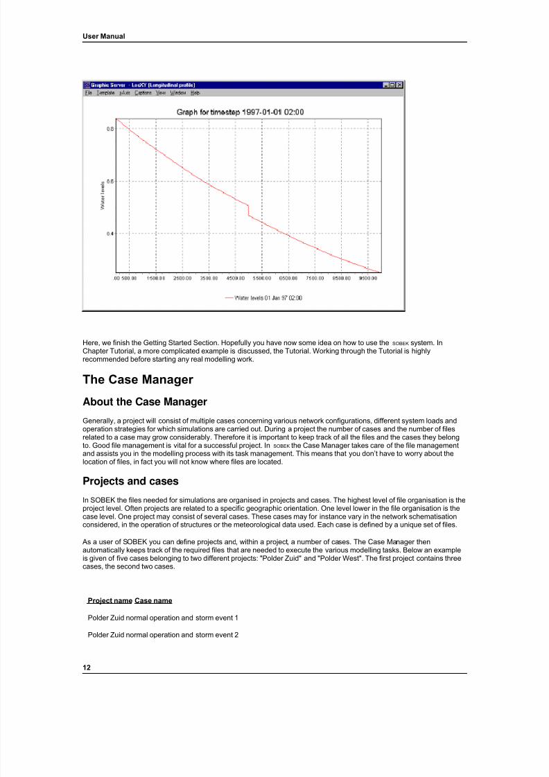
In order to get a function of place, we first select the task block 'Hydraulic Results' and choose 'F low map results'. After pressing the 'View' button ODS_View will start.
Opening window of ODS_View
For a detailed description about the functionality's and operations of ODS_View we refer to the ODS_View On LineManual. Select water level from the parameter list, select all locations, check mark the longitudinal option (below thelocation list) and select the last time step from the time steps list, and after all press 'Graph'. Now you will get the followingpicture
11
7/21/2019 SOBEK - UserManual
http://slidepdf.com/reader/full/sobek-usermanual 18/179
User Manual
Here, we finish the Getting Started Section. Hopefully you have now some idea on how to use the SOBEK system. InChapter Tutorial, a more complicated example is discussed, the Tutorial. Working through the Tutorial is highlyrecommended before starting any real modelling work.
The Case Manager
About the Case Manager
Generally, a project will consist of multiple cases concerning various network configurations, different system loads andoperation strategies for which simulations are carried out. During a project the number of cases and the number of filesrelated to a case may grow considerably. Therefore it is important to keep track of all the files and the cases they belongto. Good file management is vital for a successful project. In SOBEK the Case Manager takes care of the file managementand assists you in the modelling process with its task management. This means that you don’t have to worry about thelocation of files, in fact you will not know where files are located.
Projects and cases
In SOBEK the files needed for simulations are organised in projects and cases. The highest level of file organisation is theproject level. Often projects are related to a specific geographic orientation. One level lower in the file organisation is thecase level. One project may consist of several cases. These cases may for instance vary in the network schematisationconsidered, in the operation of structures or the meteorological data used. Each case is defined by a unique set of files.
As a user of SOBEK you can define projects and, within a project, a number of cases. The Case Manager thenautomatically keeps track of the required files that are needed to execute the various modelling tasks. Below an exampleis given of five cases belonging to two different projects: "Polder Zuid" and "Polder West". The first project contains threecases, the second two cases.
Project name Case name
Polder Zuid normal operation and storm event 1
Polder Zuid normal operation and storm event 2
12

7/21/2019 SOBEK - UserManual
http://slidepdf.com/reader/full/sobek-usermanual 19/179
User Manual
Polder Zuid adapted operation and storm event 1
Polder West normal operation and storm event 1
Polder West adapted operation and storm event 1
Project management options
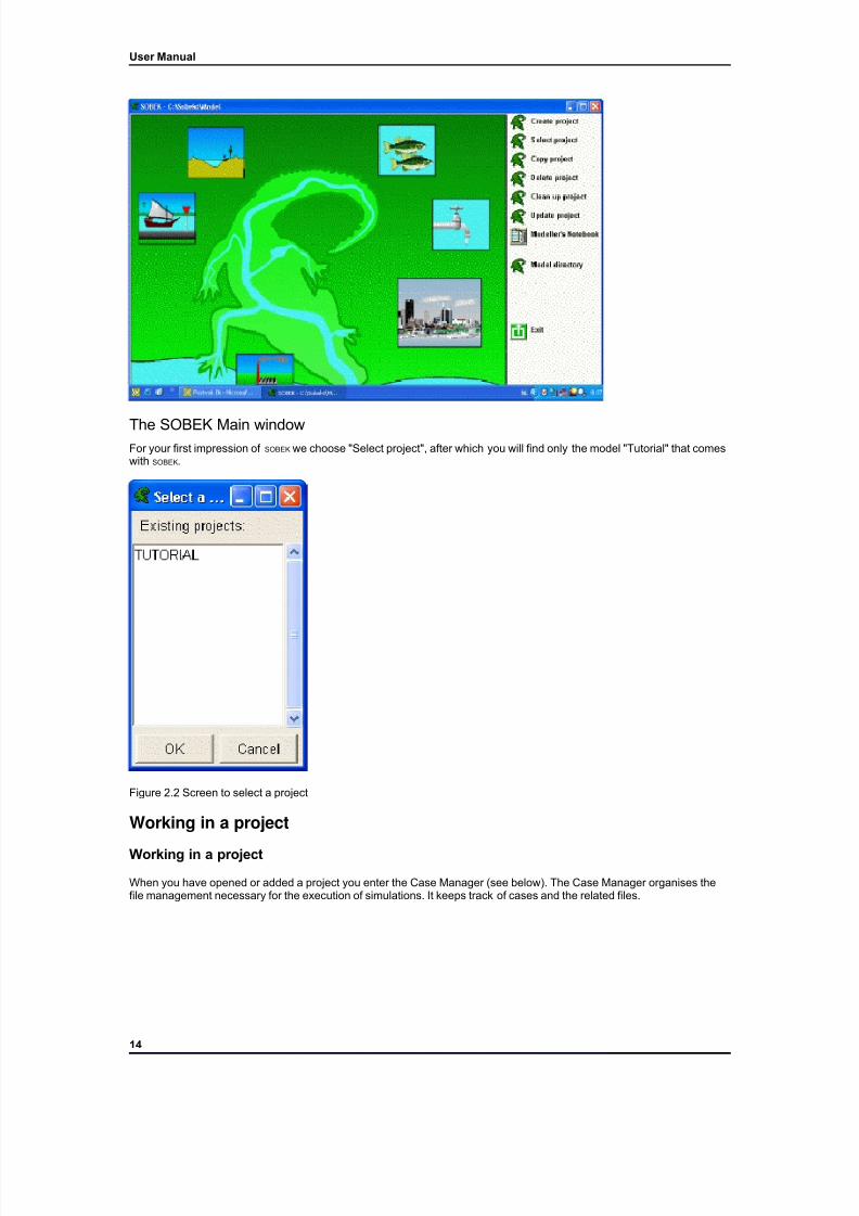
Let's start SOBEK now by double-clicking the SOBEK icon. The opening screen will look like Figure 2.1; the picture willpossibly have been adapted to your situation. In the right part of the screen you find nine icons, which represent thefollowing options:
‘Create Project ’ creates a new project on the basis of default values. You have to enter a project name of no more than 8characters. The new name is added to the project list.
‘Select Project ’ selects a project from the project list. If the list does not contain any project names first a new projectshould be created with the consists is still empty.
‘Copy Project ’ copies a project form the project list.
‘Delete Project ’ deletes a project form the project list.
‘Clean up project ’ will remove all output files from all cases of a project; a very useful option before archiving your project.
'Update Project ' updates a project from another installation. This option is used to update a complete *.SBK directorywhich has been copied from another SOBEK-installation. This option facilitates the exchange of models between differentcomputers.
Note : Update Project only works for models in version 2.50 or higher and is not downwards compatible. Soupdating from e.g. version 2.51.001 to version 2.50.039 will not work well.
‘Modellers Notebook ’ allows you to enter information on your modelling activities on the projects. It can serve as a tool toexchange information between different users working on the same projects.
‘Model directory ’ allows the user to switch from default directory for projects to load, save, update and clean up. Theselected directory is shown in the upper left corner of the window.
Note: Do not use a model directory containing a project.ini directory belonging to a different version of Sobek-RE; if you do use such a directory, you will be confronted with different versions of the User Interface, the computationalkernel, etc.
‘Exit ’ will close the SOBEK program.
The drop-down menu 'Files' at the menu-bar has only the choice 'Exit Sobek' to exit SOBEK
13
7/21/2019 SOBEK - UserManual
http://slidepdf.com/reader/full/sobek-usermanual 20/179
User Manual
The SOBEK Main windowFor your first impression of SOBEK we choose "Select project", after which you will find only the model "Tutorial" that comeswith SOBEK .
Figure 2.2 Screen to select a project
Working in a project
Working in a project
When you have opened or added a project you enter the Case Manager (see below). The Case Manager organises thefile management necessary for the execution of simulations. It keeps track of cases and the related files.
14
7/21/2019 SOBEK - UserManual
http://slidepdf.com/reader/full/sobek-usermanual 21/179
User Manual
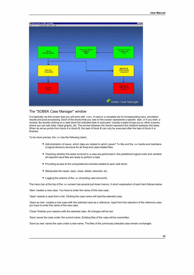
The "SOBEK Case Manager" windowIt is basically via this screen that you will work with SOBEK . A case is a complete set of corresponding input, simulationresults and post-processing. Each of the blocks that you see on the screen represents a specific task , or if you wish, amodule . By double-clicking on a task block the indicated task is executed. Usually a tasks brings you to other screens,where you can edit data, make graphs, etc. The arrows between the blocks represent the relations between the tasks.When an arrow points from block A to block B, the task of block B can only be executed after the task of block A isfinished.
To be more precise, the CMT has the following tasks:
• Administration of cases: which data are related to which cases? To this end the CMT builds and maintainsa logical directory structure for all fixed and case-related files.
• Checking whether the tasks involved in a case are performed in the predefined logical order and whether all required input files are ready to perform a task.
• Providing access to the computational modules related to each task block.
• Manipulate the cases: open, close, delete, describe, etc.
• Logging the actions of the CMT (including view and print).
The menu bar at the top of the CMT-screen has several pull-down menus. A short explanation of each item follows below.
‘New’ creates a new case. You have to enter the name of this new case.
‘Open’ selects a case from a list. Clicking the case name will load the selected case.
‘Open as new’ creates a new case with the selected case as a reference. Apart form the selection of the reference caseyou have to enter the name of the new case.
‘Close’ finishes your session with the selected case. All changes will be lost.
‘Save’ saves the case under the current name. Existing files of the case will be overwritten.
‘Save as new’ saves the case under a new name. The files of the previously selected case remain unchanged.
15
7/21/2019 SOBEK - UserManual
http://slidepdf.com/reader/full/sobek-usermanual 22/179
User Manual
‘Delete’ deletes a selected case.
‘Edit case info’ allows the user to link a "long" case description to a case.
The ‘Define Batch / Start batch’ command enables you to run a number of computations as a batch. To define a batch youmust do the following:
• Close the present case (otherwise the option Define batch is not enabled);
• Choose the option Define batch;
• Choose one or more cases from the list;
• Select the task Start model simulation;
• Choose the option Run batch from the Case menu.
The ‘Export’ command enables you to export a case to a different project.
The ‘Import’ command enables you to import a case from a different project.
The ‘Exit’ command terminates the CMT. If you want to save your work, first use ‘Save’ or ‘Save as’.
Select a menu item by clicking with the mouse, or by using the Alt-key with the underlined letter. For example, use [Alt]+[C] for Case. The Case menu provides options to operate with different cases. Some menu options may not be available.Inactive options are shown dimmed (grey).
The Modelling Tasks
Once you have defined a case, through the options mentioned above (or by clicking on one of the task blocks), your modelling work is structured in tasks which have to be carried out in a certain order. The tasks are:
• Process Library Configuration Tool :definition of processes for water quality
• Process Library Configuration Editor :definition of parameters for water quality
• Model Schematisation:via this block you get access to all screens that are needed to enter your input and to give control data for the computations to make.
• Hydraulic computation:the computation of water flow, salinity, sediment and morphology ( depending on which of thephenomena you take into account).
• Hydraulic Results:graphs and export into files of result data
• Hydraulic and Water Quality computation.
• Hydraulic & Water Quality Results:
graphs and export into files of result data
Colours
The Case Manager keeps track of the task status and shows the status of each task by means of the following colours:
grey: no case selected or defined yet;
yellow: the task can be executed;
purple: the task is running;
16
7/21/2019 SOBEK - UserManual
http://slidepdf.com/reader/full/sobek-usermanual 23/179
User Manual
green: the task has been executed at least once and can be executed again;
red: the task cannot be executed until the preceding task has been executed.
So when you enter the CMT-screen all blocks will be grey until you have selected a case.
Activating a task
To activate any task block, you first have to open a case via the menu bar (under ‘Case’). You can also double-click oneof the grey task blocks and select a case from the list that pops up. To execute a task (yellow or green) you double-clickits block, after which this becomes purple and finally green.
Additional functions on task blocks
By clicking on a task block with the right-hand mouse button you get access to help screens, logging files produced duringthe execution of a task and in some cases special functions. Logging files can only be addressed when the task is finished(green).
The 'Model Schematisation' task has the following additional functions:
• Help: to get the SOBEK-RE Help (Also possible by Help on the CMT-Menu).
• Cut Schematisation : to start cutting schematisation.
• Show Cut Messages: to view to message files from the cutting
• Combine Schematisation : to combine to schematisations together.
• Show Combine Messages: to view to message files from the merge
• Graded sediment Input File: to edit the Graded Sediment Input File. For Graded Sediment there is aspecial manual available.
The 'Hydraulic and Water Quality Computation' task has the following additional functions:
• Help: to get the SOBEK-RE Help (Also possible by Help on the CMT-Menu).
• Copy restart Files: for the use of this see the Appendix about Restart
• Activate Graded Sediment: to switch on Graded Sediment calculations (See Graded Sediment manual)
• Deactivate Graded Sediment: to switch off Graded Sediment calculations (See Graded Sediment manual)
In case of the 'Hydraulic and Water Quality Computation' Tasks you also get the option 'Copy restart Files'.
Processes Library
Processes Library Configuration Tool
Processes Library Configuration Tool
You can set or change the configuration of the Processes Library with the help of the Processes Library ConfigurationTool (also called "PLCT"). The PLCT will need some time to load its input tables. Next, you will see the "Water Quality"window and the "Substance Groups" window appear. The configuration of the Processes Library is arranged in differentsteps.
The Selection of Active Substance Groups
This is done in the "Substance Groups" window (Figure 2.1).
17
7/21/2019 SOBEK - UserManual
http://slidepdf.com/reader/full/sobek-usermanual 24/179
User Manual
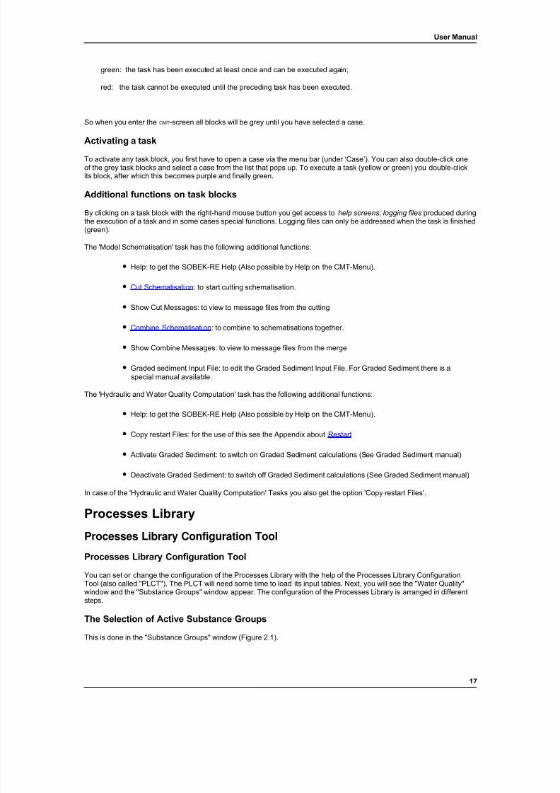
Figure 2.1: The "Substance Groups" window.
• Click an item in the "Available Substance Groups" list to place it on the "Selected Substance Groups" list.
• Click a selected item in the "Available Substance Groups" list while holding the [Ctrl] key to remove it fromthe "Selected Substance Groups" list.
• Click an unselected item in the "Available Substance Groups" list while holding the [Ctrl] key to add it tothe "Selected Substance Groups" list.
Selection of "State Variables" or "Substances" within a group
• Click an item in the "Selected Substance Groups" list. The "Select Substances" window appears (Figure2.2).
18
7/21/2019 SOBEK - UserManual
http://slidepdf.com/reader/full/sobek-usermanual 25/179
User Manual
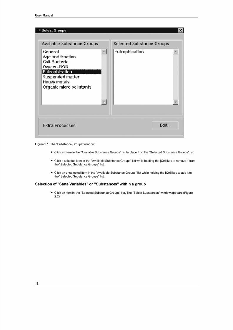
Figure 2.2: The "Select Substances" window.
• Click an item in the "Available Substances" list to place it on the "Selected Substances" list.
• Click a selected item in the "Available Substances" list while holding the [Ctrl] key to remove it from the"Selected Substances" list.
• Click an unselected item in the "Available Substances" list while holding the [Ctrl] key to add it to the"Selected Substances" list.
• Click <Ready> to return to the "Substances Groups" window.
Selection of Water Quality Processes Affecting the State variables
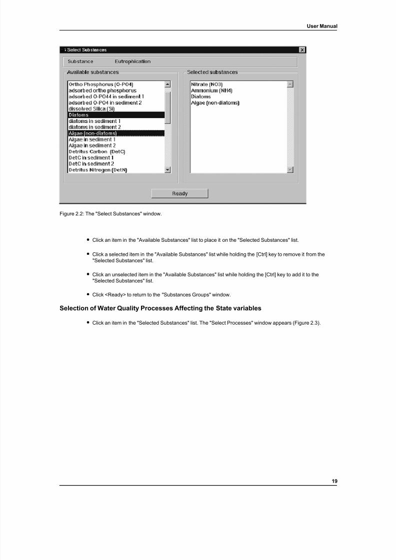
• Click an item in the "Selected Substances" list. The "Select Processes" window appears (Figure 2.3).
19
7/21/2019 SOBEK - UserManual
http://slidepdf.com/reader/full/sobek-usermanual 26/179
User Manual
Figure 2.3: The "Select Processes" window.
The "Select Processes" window lists all processes which directly affect a state variable.
• Click on the tick box(es) corresponding to the desired process(es) to activate them. An <Edit> or <Specify> button appears. <Edit> indicates an optional further specification of that process, whereas<Specify> indicates an obligatory action.
Specifying or Editing a Process
• Click on the <Edit> or <Specify> button behind an activated process. The "Specify Process" windowappears (Figure 2.4).
20

7/21/2019 SOBEK - UserManual
http://slidepdf.com/reader/full/sobek-usermanual 27/179
User Manual
Figure 2.4: The "Specify Process" window.
The "Specify Process" window lists all input and output parameters of the process. For the input parameters the followingpossibilities exist:
• The item is "modeled": this holds for the active state variables, the meteo functions (radiation, windvelocity, temperature) and the hydraulical functions (horizontal surface, width, Chézy coefficient and
stream flow velocity). No actions are needed/possible.
• The item is "constant" with a default value:
• use the list box to see if the item can be produced by another process, and to switch the item to "process";
• click the "Editable" tick box to optionally include it in the list of process parameters you are going to editlater on;
• click the "Output" tick box to optionally include it in the water quality model output files.
• The item is "constant" with "no default" available:
• use the list box to see if the item can be produced by another process, and to switch the item to "process";
• click the "Editable" tick box to include it in the list of process parameters you are going to edit later on(obligatory!!);
• click the "Output" tick box to optionally include it in the water quality model output files.
• The item is the output from another "process":
• use the list box to switch the item to "constant";
• click the "Output" tick box to optionally include it in the water quality model output files.
For the output parameters:
21
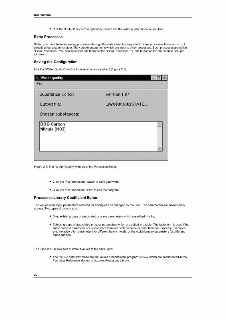
7/21/2019 SOBEK - UserManual
http://slidepdf.com/reader/full/sobek-usermanual 28/179
User Manual
• click the "Output" tick box to optionally include it in the water quality model output files.
Extra Processes
So far, you have been accessing processes through the state variables they affect. Some processes however, do notdirectly affect a state variable. They create output items which are input to other processes. Such processes are called"Extra Processes". You can specify or edit them via the "Extra Processes:" <Edit> button on the "Substance Groups"window.
Saving the Configuration
Use the "Water Quality" window to save your work and exit (Figure 2.5).
Figure 2.5: The "Water Quality" window of the Processes Editor.
• Click the "File" menu and "Save" to save your work.
• Click the "File" menu and "Exit" to end the program.
Processes Library Coefficient Editor
The values of all input parameters selected for editing can be changed by the user. The parameters are presented ingroups. Two types of groups exist:
• Simple lists: groups of associated process parameters which are edited in a list.
• Tables: groups of associated process parameters which are edited in a table. The table form is used if thesame process parameter occurs for more than one state variable or more than one process. Examplesare: the adsorption parameters for different heavy metals, or the stoichiometry parameters for differentalgae species.
The user can use two sets of default values to fall back upon:
• The " DELWAQ defaults": these are the values present in the program DELWAQ , which are documented in theTechnical Reference Manual of DELWAQ ’s Processes Library.
22
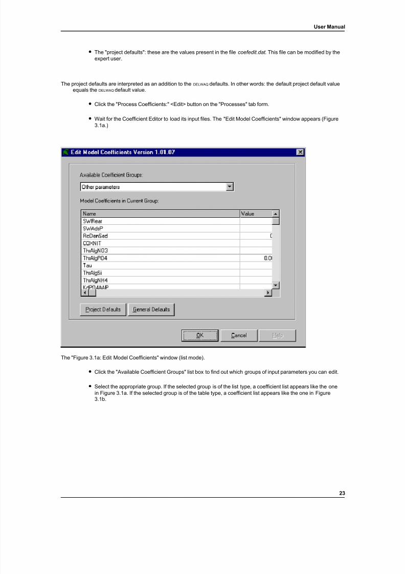
7/21/2019 SOBEK - UserManual
http://slidepdf.com/reader/full/sobek-usermanual 29/179
User Manual
• The "project defaults": these are the values present in the file coefedit.dat . This file can be modified by theexpert user.
The project defaults are interpreted as an addition to the DELWAQ defaults. In other words: the default project default valueequals the DELWAQ default value.
• Click the "Process Coefficients:" <Edit> button on the "Processes" tab form.
• Wait for the Coefficient Editor to load its input files. The "Edit Model Coefficients" window appears (Figure3.1a.)
The "Figure 3.1a: Edit Model Coefficients" window (list mode).
• Click the "Available Coefficient Groups" list box to find out which groups of input parameters you can edit.
• Select the appropriate group. If the selected group is of the list type, a coefficient list appears like the onein Figure 3.1a. If the selected group is of the table type, a coefficient list appears like the one in Figure3.1b.
23
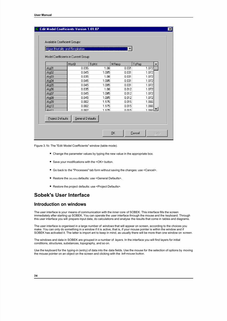
7/21/2019 SOBEK - UserManual
http://slidepdf.com/reader/full/sobek-usermanual 30/179
User Manual
Figure 3.1b: The "Edit Model Coefficients" window (table mode).
• Change the parameter values by typing the new value in the appropriate box.
• Save your modifications with the <OK> button.
• Go back to the "Processes" tab form without saving the changes: use <Cancel>.
• Restore the DELWAQ defaults: use <General Defaults>.
• Restore the project defaults: use <Project Defaults>.
Sobek's User Interface
Introduction on windows
The user interface is your means of communication with the inner core of SOBEK. This interface fills the screenimmediately after starting up SOBEK. You can operate the user interface through the mouse and the keyboard. Throughthis user interface you will prepare input data, do calculations and analyse the results that come in tables and diagrams.
The user interface is organised in a large number of windows that will appear on screen, according to the choices youmake. You can only do something in a window if it is active, that is, if your mouse pointer is within the window and if SOBEK has activated it. The latter is import ant to keep in mind, as usually there will be more than one window on screen.
The windows and data in SOBEK are grouped in a number of layers . In the interface you will find layers for initialconditions, structures, substances, topography, and so on.
Use the keyboard for the typing-in (entry) of data into the data fields. Use the mouse for the selection of options by movingthe mouse pointer on an object on the screen and clicking with the left mouse button.
24
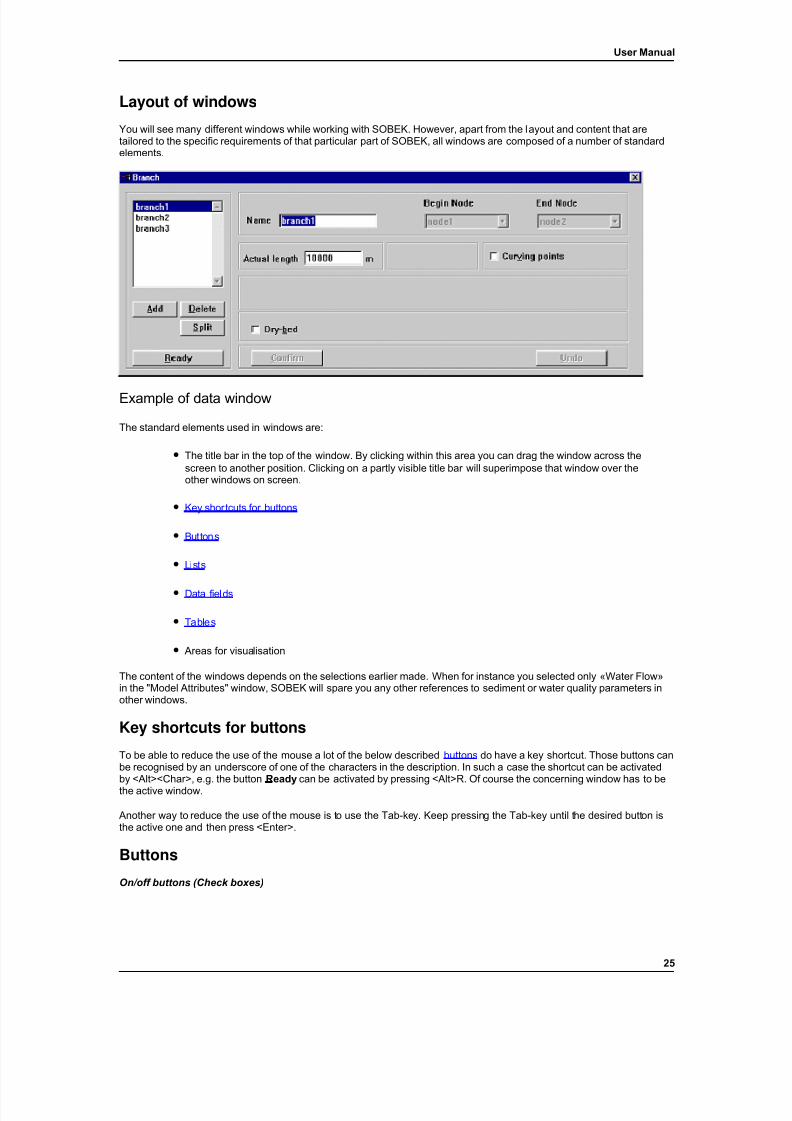
7/21/2019 SOBEK - UserManual
http://slidepdf.com/reader/full/sobek-usermanual 31/179
User Manual
Layout of windows
You will see many different windows while working with SOBEK. However, apart from the layout and content that aretailored to the specific requirements of that particular part of SOBEK, all windows are composed of a number of standardelements.
Example of data window
The standard elements used in windows are:
• The title bar in the top of the window. By clicking within this area you can drag the window across thescreen to another position. Clicking on a partly visible title bar will superimpose that window over theother windows on screen.
• Key shortcuts for buttons
• Buttons
• Lists
• Data fields
• Tables
• Areas for visualisation
The content of the windows depends on the selections earlier made. When for instance you selected only «Water Flow»in the "Model Attributes" window, SOBEK will spare you any other references to sediment or water quality parameters inother windows.
Key shortcuts for buttons
To be able to reduce the use of the mouse a lot of the below described buttons do have a key shortcut. Those buttons canbe recognised by an underscore of one of the characters in the description. In such a case the shortcut can be activatedby <Alt><Char>, e.g. the button Ready can be activated by pressing <Alt>R. Of course the concerning window has to bethe active window.
Another way to reduce the use of the mouse is to use the Tab-key. Keep pressing the Tab-key until the desired button isthe active one and then press <Enter>.
Buttons
On/off buttons (Check boxes)
25
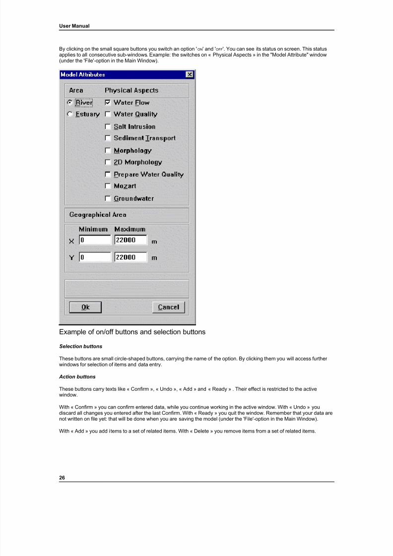
7/21/2019 SOBEK - UserManual
http://slidepdf.com/reader/full/sobek-usermanual 32/179
User Manual
By clicking on the small square buttons you switch an option ' ON ' and ' OFF '. You can see its status on screen. This statusapplies to all consecutive sub-windows. Example: the switches on « Physical Aspects » in the "Model Attribute" window(under the 'File'-option in the Main Window).
Example of on/off buttons and selection buttons
Selection buttons
These buttons are small circle-shaped buttons, carrying the name of the option. By clicking them you will access further windows for selection of items and data entry.
Action buttons
These buttons carry texts like « Confirm », « Undo », « Add » and « Ready » . Their effect is restricted to the activewindow.
With « Confirm » you can confirm entered data, while you continue working in the active window. With « Undo » youdiscard all changes you entered after the last Confirm. With « Ready » you quit the window. Remember that your data arenot written on file yet: that will be done when you are saving the model (under the 'File'-option in the Main Window).
With « Add » you add i tems to a set of related items. With « Delete » you remove items from a set of related items.
26
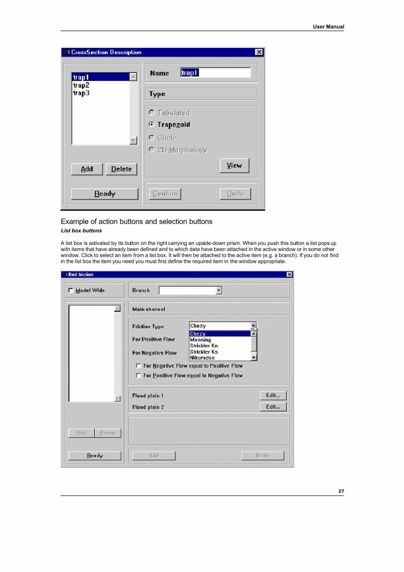
7/21/2019 SOBEK - UserManual
http://slidepdf.com/reader/full/sobek-usermanual 33/179
User Manual
Example of action buttons and selection buttonsList box buttons
A list box is activated by its button on the right carrying an upside-down prism. When you push this button a list pops upwith items that have already been defined and to which data have been attached in the active window or in some other window. Click to select an item from a list box. It will then be attached to the active item (e.g. a branch). If you do not findin the list box the item you need you must first define the required item in the window appropriate.
27
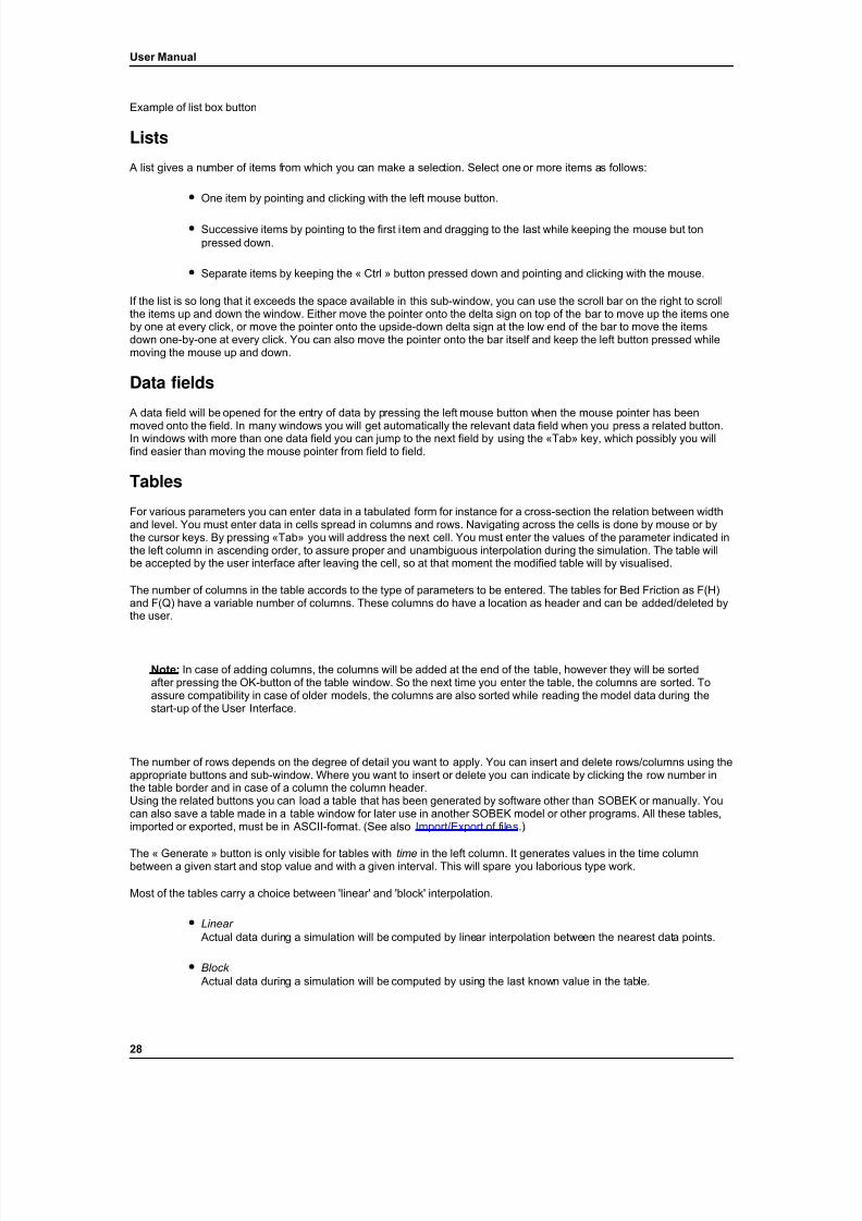
7/21/2019 SOBEK - UserManual
http://slidepdf.com/reader/full/sobek-usermanual 34/179
User Manual
Example of list box button
Lists
A list gives a number of items from which you can make a selection. Select one or more items as follows:
• One item by pointing and clicking with the left mouse button.
• Successive items by pointing to the first item and dragging to the last while keeping the mouse but tonpressed down.
• Separate items by keeping the « Ctrl » button pressed down and pointing and clicking with the mouse.
If the list is so long that it exceeds the space available in this sub-window, you can use the scroll bar on the right to scrollthe items up and down the window. Either move the pointer onto the delta sign on top of the bar to move up the items oneby one at every click, or move the pointer onto the upside-down delta sign at the low end of the bar to move the itemsdown one-by-one at every click. You can also move the pointer onto the bar itself and keep the left button pressed whilemoving the mouse up and down.
Data fields
A data field will be opened for the entry of data by pressing the left mouse button when the mouse pointer has been
moved onto the field. In many windows you will get automatically the relevant data field when you press a related button.In windows with more than one data field you can jump to the next field by using the «Tab» key, which possibly you willfind easier than moving the mouse pointer from field to field.
Tables
For various parameters you can enter data in a tabulated form for instance for a cross-section the relation between widthand level. You must enter data in cells spread in columns and rows. Navigating across the cells is done by mouse or bythe cursor keys. By pressing «Tab» you will address the next cell. You must enter the values of the parameter indicated inthe left column in ascending order, to assure proper and unambiguous interpolation during the simulation. The table willbe accepted by the user interface after leaving the cell, so at that moment the modified table will by visualised.
The number of columns in the table accords to the type of parameters to be entered. The tables for Bed Friction as F(H)and F(Q) have a variable number of columns. These columns do have a location as header and can be added/deleted bythe user.
Note: In case of adding columns, the columns will be added at the end of the table, however they will be sortedafter pressing the OK-button of the table window. So the next time you enter the table, the columns are sorted. Toassure compatibility in case of older models, the columns are also sorted while reading the model data during thestart-up of the User Interface.
The number of rows depends on the degree of detail you want to apply. You can insert and delete rows/columns using theappropriate buttons and sub-window. Where you want to insert or delete you can indicate by clicking the row number inthe table border and in case of a column the column header.Using the related buttons you can load a table that has been generated by software other than SOBEK or manually. Youcan also save a table made in a table window for later use in another SOBEK model or other programs. All these tables,imported or exported, must be in ASCII-format. (See also Import/Export of files .)
The « Generate » button is only visible for tables with time in the left column. It generates values in the time columnbetween a given start and stop value and with a given interval. This will spare you laborious type work.
Most of the tables carry a choice between 'linear' and 'block' interpolation.
• Linear Actual data during a simulation will be computed by linear interpolation between the nearest data points.
• Block Actual data during a simulation will be computed by using the last known value in the table.
28
7/21/2019 SOBEK - UserManual
http://slidepdf.com/reader/full/sobek-usermanual 35/179
User Manual
Besides interpolation, extrapolation is sometimes necessary. For instance a timetable with lateral inflow may cover aperiod less than the computational period. In that case the table is extrapolated by keeping the last/first given value. Thisprinciple also applies for tables that are place or height related instead of time-related.
Insensitive buttons and data fields
You can only use buttons and data fields when their use is logical within SOBEK. When for instance you are enteringdata for a cross-section you have no access to another cross-section before you finish the active one by « add »,« confirm » (or « undo »). Some buttons and data fields are made insensitive by SOBEK. They do not react when youtry to access them with the mouse. You can see which parts of a window are insensitive by their shaded appearance.Remember: SOBEK does this for your convenience. It keeps track of your actions and thus presents the appropriateoptions only.
Important windows
The "SOBEK-model" window is on screen as long as you are working in the SOBEK User Interface. It appears after youhave activated the 'Schematisation Task' of the Case Management Tool and begin building a new model, or modifyingexisting model. It shows a continuously updated model network.
The second window that is always on screen is the "Layer" window. By clicking the Radio Buttons the user can selectwhich layer he wants to work with. With the Check Boxes the layer items can be visualised in the Model Window. In this
way it can be seen if data for a certain layer in a node/branch is given.
The third window that is always on screen is the "Message" window. It shows messages, warnings and errors during aSOBEK session.
The other windows vary with the physical processes and the options that are switched on. Their content is described inthe remainder of this chapter.
Formats
Numeric format
The numeric format of data to be entered is free as far as the number of digits after the decimal point is concerned.Remember: In the English language one uses the decimal point, not the decimal comma. Scientific notation is accepted.
Be careful that you use the units that are indicated to the right of a data field.
Date and time
Date and time have to be indicated with the format as in the following example (note the ' ;' between date and time):
1995/12/20;18:12:00
which represents 1995, December 20, twelve past six in the afternoon.
The date can be omitted. Note the format, which is year/month/date . The time must comprise the complete formathours:minutes:seconds.
In tables you do not need to type the complete format in every entry. After you entered the first value in full format you cancontinue with following entries by typing only a part of the full format. SOBEK uses the following interpretation (with theabove entry as reference):
Type: 15: You get the next 'minute' value: 1995/12/20;18:15:00
Type: 19:00: You get the next 'hour' value: 1995/12/20;19:12:00
Type: 21;00:00: You get the next 'day' value: 1995/12/21;18:12:00
29
7/21/2019 SOBEK - UserManual
http://slidepdf.com/reader/full/sobek-usermanual 36/179
User Manual
Default values
For various parameters SOBEK places default values in the corresponding data screen or data table. They representcommonly accepted values or plausible first guesses for those parameters. However, you may change them if you thinkthey are not appropriate for the situation in your model. For several data, e.g. friction, initial condition, sediment transportformulae and meteo data you can define defaults for your model by using the « Model Wide » option.
Descriptions of windowsBelow you find the descriptions of the principal windows of the interface. They are grouped as follows:
• SOBEK-model window.
• Windows related to each of the data layers in the user interface. The text is related to the full content of awindow, that is, as if all physical aspects are switched on.
• Post-processing.
Sobek Model Window
Sobek-model window
The "SOBEK-model" window appears after starting the SOBEK User Interface. A model is an application of SOBEK: itcontains the network of nodes and branches, the hydraulic structures, cross-sections, related data, etc, that together formthe computer simulation of a real situation.
The "SOBEK-model" window is split in two parts. The upper part is a menu bar and offers the following main choices:
• File
• With 'Save Model' you save the modified Model Data.
• Under ' Model Attributes ' you determine what physical aspects you want to include. This window isdescribed separately below.
• With 'Exit' you leave the Schematisation Task. When you exit the Schematisation Task without previouslyhaving saved the model, a special window will appear to Save the model, to Discard the modifications or toCancel the Exit.
• Settings
• By clicking on 'Lists in Alphabetical Order' you can change the order in which the items in the choice listsare presented. When the check mark is on the lists are presented in alphabetical order, otherwise indatabase order. The current setting is stored when the SOBEK-Model window is closed.
• View
• With 'Zoom' you can enlarge a part of the displayed network by pointing to the upper left corner of thezoomed area and, while keeping the left mouse button pressed, move to the lower right corner of the areaand release the mouse button. With 'Reset' you return to the initial display size.
• Operations
• 'Validate model ' checks the consistency of the model and if it is complete. Messages are displayed in the"Special messages" window.
• 'Select Schematisation ' is used to select a part of the model schematisation for cutting .
• 'Remove prefixes ' removes prefixes of SOBEK Data Object names. This option can be used to remove theprefix 'P_' (default) which is put before the names during combining models . During the removal of theprefix it is checked if the name without the prefix is still unique and if not the prefix will not be removed.
After the removal a report is shown with the results of the removal action. By selecting the text andpressing <Ctrl>C (Copy) the report text can be put into the Clipboard for later use, e.g. saving into a textfile for later use.
30

7/21/2019 SOBEK - UserManual
http://slidepdf.com/reader/full/sobek-usermanual 37/179
User Manual
• Help
• With 'Contents' you get the "SOBEK help" window. By clicking and scrolling you can access the list of keywords and contents of the Reference Manual. If you want to know how to use the SOBEK help functionyou can either use the «F1» function key from here or choose the 'How to use Help' option from the menu.
The lower part displays the actual lay-out of the network. What more it can show than the basic network of nodes and
branches, depends on the layers you have switched on in the window "Select Layers". In the displayed network you canpoint and click with the mouse on nodes, branches and structures. If the corresponding window is active you get all datarelated to the clicked object in the data fields of that window. As long as you are in that window you can also drag objects(a structure for instance) to a new position by clicking the new position with the right hand mouse button and then click «Confirm » in the related active window.
Model Attributes
Before you start a new model you must select some basic items in the « Model Attributes » screen. The item that youselect in the field « Area Class » and « Physical Aspects » determines the options that you will see and have access to inthe remaining screens. If you select for instance « River », « Water Flow » and « Morphology » only those options will beavailable in windows that are relevant to a river morphology problem.
You will notice that some options are coupled and switched on automatically. Morphology for instance cannot be activewithout Sediment Transport and Water Flow, Salt Intrusion not without Water Flow.
Water Quality can not be active without Prepare Water Quality and Water Flow.
Once you have started a model the selected physical aspects can be changed. If you change the set of physical aspectsyou want to take into account, this will have an influence on the layer structure , and on the simulations that you ran for theoriginal layer structure.
You are warned against loss of data while changing the set of physical aspects in the window "Layer version informationloss". This window pops up when you save a version of the model with a modified layer version.
Under "Geographical Area" you specify the boundary co-ordinates (in m) of the window showing the layout of the model.
31
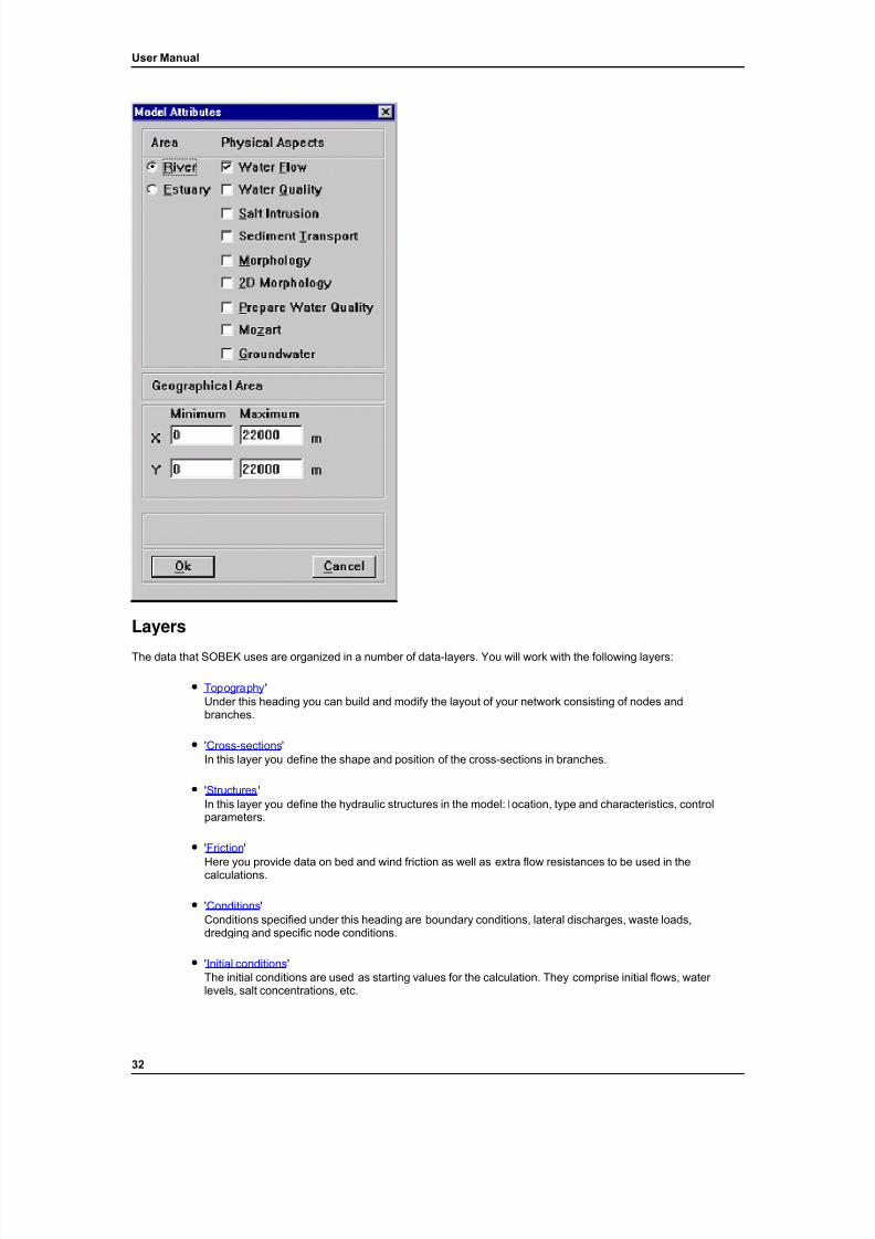
7/21/2019 SOBEK - UserManual
http://slidepdf.com/reader/full/sobek-usermanual 38/179
User Manual
Layers
The data that SOBEK uses are organized in a number of data-layers. You will work with the following layers:
• Topography 'Under this heading you can build and modify the layout of your network consisting of nodes andbranches.
• 'Cross-sections 'In this layer you define the shape and position of the cross-sections in branches.
• 'Structures 'In this layer you define the hydraulic structures in the model: location, type and characteristics, controlparameters.
• 'Friction 'Here you provide data on bed and wind friction as well as extra flow resistances to be used in thecalculations.
• 'Conditions 'Conditions specified under this heading are boundary conditions, lateral discharges, waste loads,dredging and specific node conditions.
• 'Initial conditions 'The initial conditions are used as starting values for the calculation. They comprise initial flows, water levels, salt concentrations, etc.
32
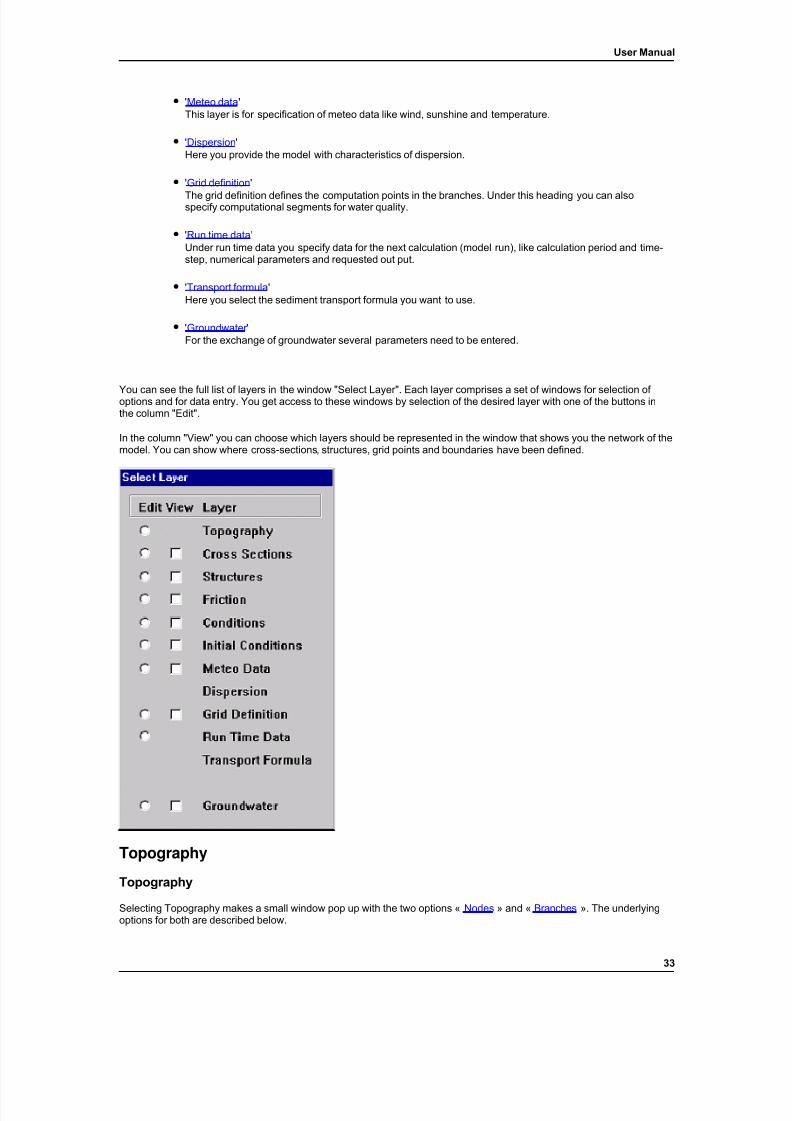
7/21/2019 SOBEK - UserManual
http://slidepdf.com/reader/full/sobek-usermanual 39/179
User Manual
• 'Meteo data 'This layer is for specification of meteo data like wind, sunshine and temperature.
• 'Dispersion 'Here you provide the model with characteristics of dispersion.
• 'Grid definition '
The grid definition defines the computation points in the branches. Under this heading you can alsospecify computational segments for water quality.
• 'Run time data 'Under run time data you specify data for the next calculation (model run), like calculation period and time-step, numerical parameters and requested out put.
• 'Transport formula 'Here you select the sediment transport formula you want to use.
• 'Groundwater 'For the exchange of groundwater several parameters need to be entered.
You can see the full list of layers in the window "Select Layer". Each layer comprises a set of windows for selection of options and for data entry. You get access to these windows by selection of the desired layer with one of the buttons inthe column "Edit".
In the column "View" you can choose which layers should be represented in the window that shows you the network of themodel. You can show where cross-sections, structures, grid points and boundaries have been defined.
Topography
Topography
Selecting Topography makes a small window pop up with the two options « Nodes » and « Branches ». The underlyingoptions for both are described below.
33
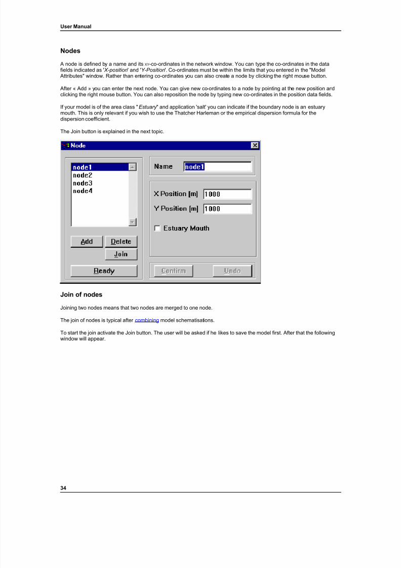
7/21/2019 SOBEK - UserManual
http://slidepdf.com/reader/full/sobek-usermanual 40/179
User Manual
Nodes
A node is defined by a name and its XY-co-ordinates in the network window. You can type the co-ordinates in the datafields indicated as ' X-position ' and ' Y-Position '. Co-ordinates must be within the limits that you entered in the "Model
Attributes" window. Rather than entering co-ordinates you can also create a node by clicking the right mouse button.
After « Add » you can enter the next node. You can give new co-ordinates to a node by pointing at the new position andclicking the right mouse button. You can also reposition the node by typing new co-ordinates in the position data fields.
If your model is of the area class " Estuary " and application 'salt' you can indicate if the boundary node is an estuarymouth. This is only relevant if you wish to use the Thatcher Harleman or the empirical dispersion formula for thedispersion coefficient.
The Join button is explained in the next topic.
Join of nodes
Joining two nodes means that two nodes are merged to one node.
The join of nodes is typical after combining model schematisations.
To start the join activate the Join button. The user will be asked if he likes to save the model first. After that the followingwindow will appear.
34
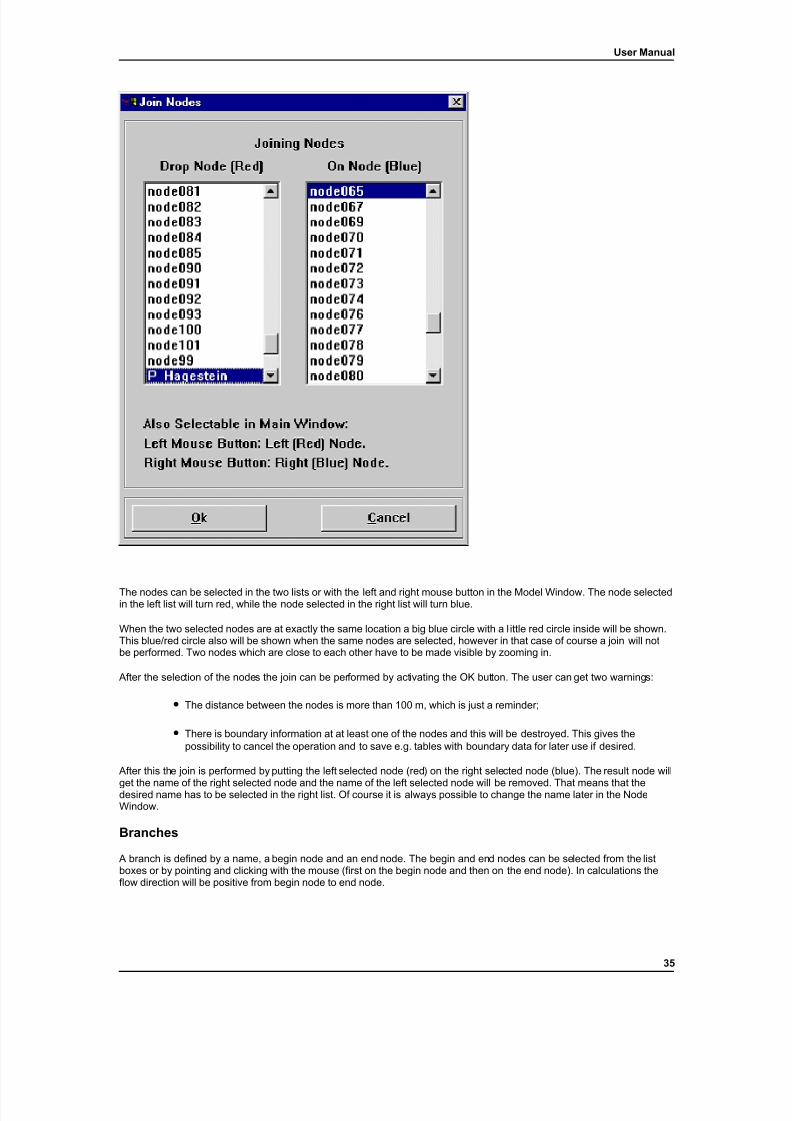
7/21/2019 SOBEK - UserManual
http://slidepdf.com/reader/full/sobek-usermanual 41/179
User Manual
The nodes can be selected in the two lists or with the left and right mouse button in the Model Window. The node selectedin the left list will turn red, while the node selected in the right list will turn blue.
When the two selected nodes are at exactly the same location a big blue circle with a l ittle red circle inside will be shown.This blue/red circle also will be shown when the same nodes are selected, however in that case of course a join will notbe performed. Two nodes which are close to each other have to be made visible by zooming in.
After the selection of the nodes the join can be performed by activating the OK button. The user can get two warnings:
• The distance between the nodes is more than 100 m, which is just a reminder;
• There is boundary information at at least one of the nodes and this will be destroyed. This gives thepossibility to cancel the operation and to save e.g. tables with boundary data for later use if desired.
After this the join is performed by putting the left selected node (red) on the right selected node (blue). The result node will
get the name of the right selected node and the name of the left selected node will be removed. That means that thedesired name has to be selected in the right list. Of course it is always possible to change the name later in the NodeWindow.
Branches
A branch is defined by a name, a begin node and an end node. The begin and end nodes can be selected from the listboxes or by pointing and clicking with the mouse (first on the begin node and then on the end node). In calculations theflow direction will be positive from begin node to end node.
35
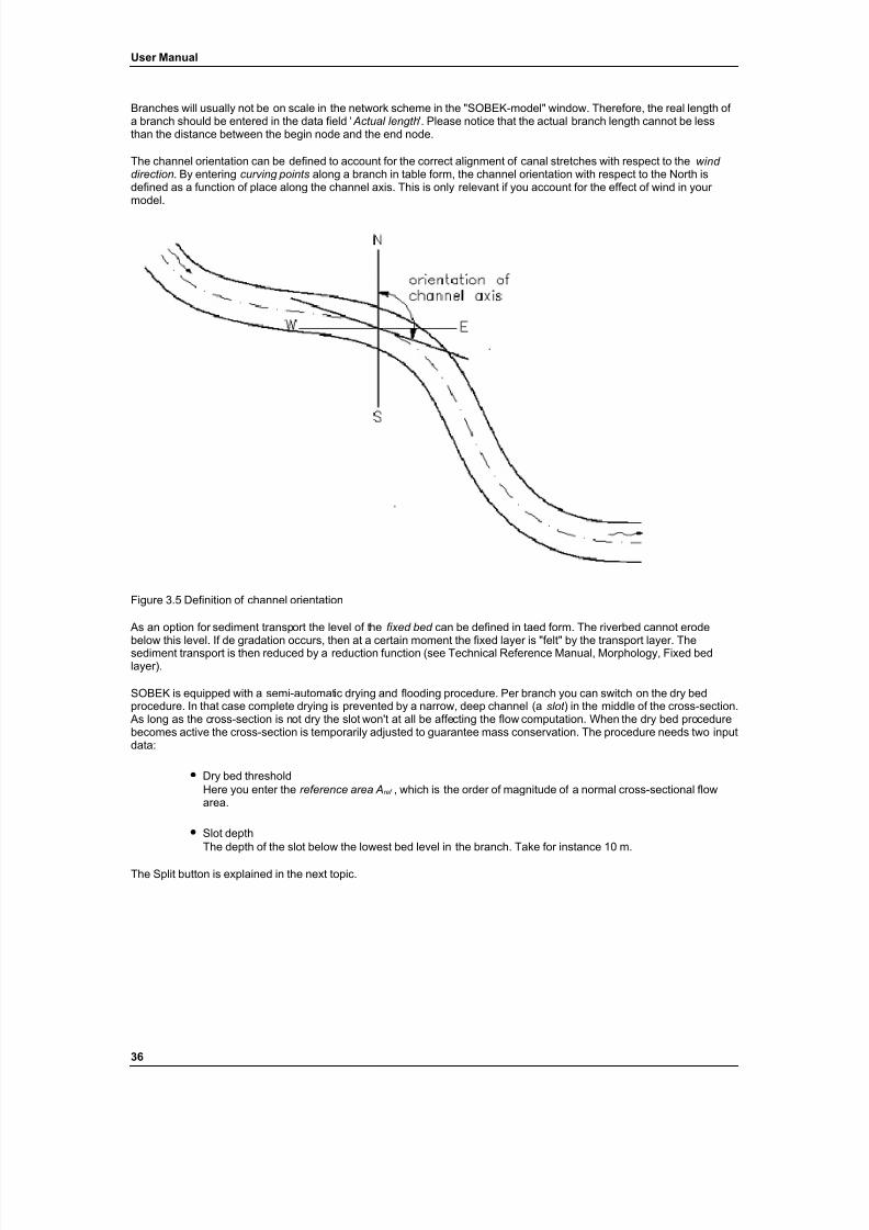
7/21/2019 SOBEK - UserManual
http://slidepdf.com/reader/full/sobek-usermanual 42/179
User Manual
Branches will usually not be on scale in the network scheme in the "SOBEK-model" window. Therefore, the real length of a branch should be entered in the data field ' Actual length '. Please notice that the actual branch length cannot be lessthan the distance between the begin node and the end node.
The channel orientation can be defined to account for the correct alignment of canal stretches with respect to the wind direction . By entering curving points along a branch in table form, the channel orientation with respect to the North isdefined as a function of place along the channel axis. This is only relevant if you account for the effect of wind in your model.
Figure 3.5 Definition of channel orientation
As an option for sediment transport the level of the fixed bed can be defined in taed form. The riverbed cannot erodebelow this level. If de gradation occurs, then at a certain moment the fixed layer is "felt" by the transport layer. Thesediment transport is then reduced by a reduction function (see Technical Reference Manual, Morphology, Fixed bedlayer).
SOBEK is equipped with a semi-automatic drying and flooding procedure. Per branch you can switch on the dry bedprocedure. In that case complete drying is prevented by a narrow, deep channel (a slot ) in the middle of the cross-section.
As long as the cross-section is not dry the slot won't at all be affecting the flow computation. When the dry bed procedurebecomes active the cross-section is temporarily adjusted to guarantee mass conservation. The procedure needs two inputdata:
• Dry bed thresholdHere you enter the reference area A ref , which is the order of magnitude of a normal cross-sectional flowarea.
• Slot depthThe depth of the slot below the lowest bed level in the branch. Take for instance 10 m.
The Split button is explained in the next topic.
36
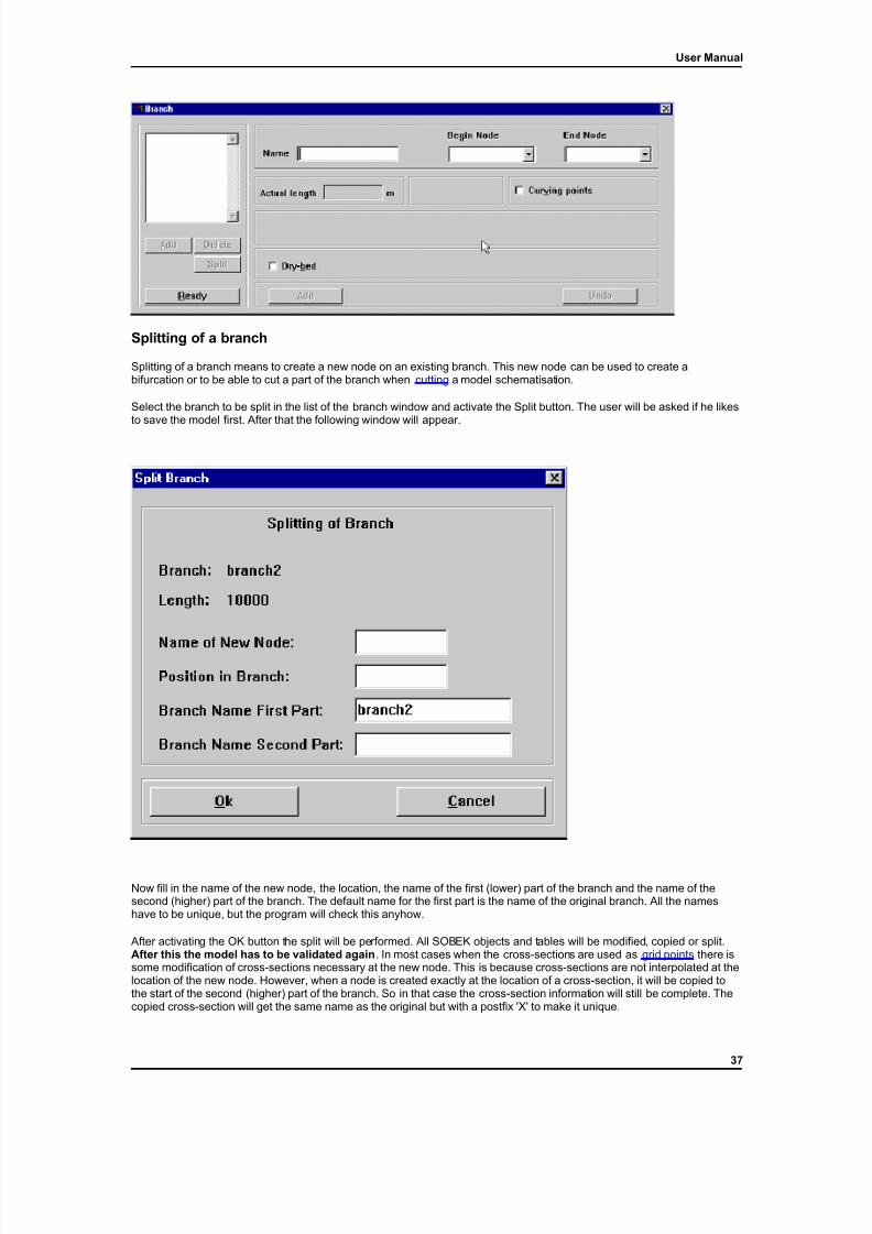
7/21/2019 SOBEK - UserManual
http://slidepdf.com/reader/full/sobek-usermanual 43/179
User Manual
Splitting of a branch
Splitting of a branch means to create a new node on an existing branch. This new node can be used to create abifurcation or to be able to cut a part of the branch when cutting a model schematisation.
Select the branch to be split in the list of the branch window and activate the Split button. The user will be asked if he likesto save the model first. After that the following window will appear.
Now fill in the name of the new node, the location, the name of the first (lower) part of the branch and the name of thesecond (higher) part of the branch. The default name for the first part is the name of the original branch. All the nameshave to be unique, but the program will check this anyhow.
After activating the OK button the split will be performed. All SOBEK objects and tables will be modified, copied or split.After this the model has to be validated again . In most cases when the cross-sections are used as grid points there issome modification of cross-sections necessary at the new node. This is because cross-sections are not interpolated at thelocation of the new node. However, when a node is created exactly at the location of a cross-section, it will be copied tothe start of the second (higher) part of the branch. So in that case the cross-section information will still be complete. Thecopied cross-section will get the same name as the original but with a postfix 'X' to make it unique.
37
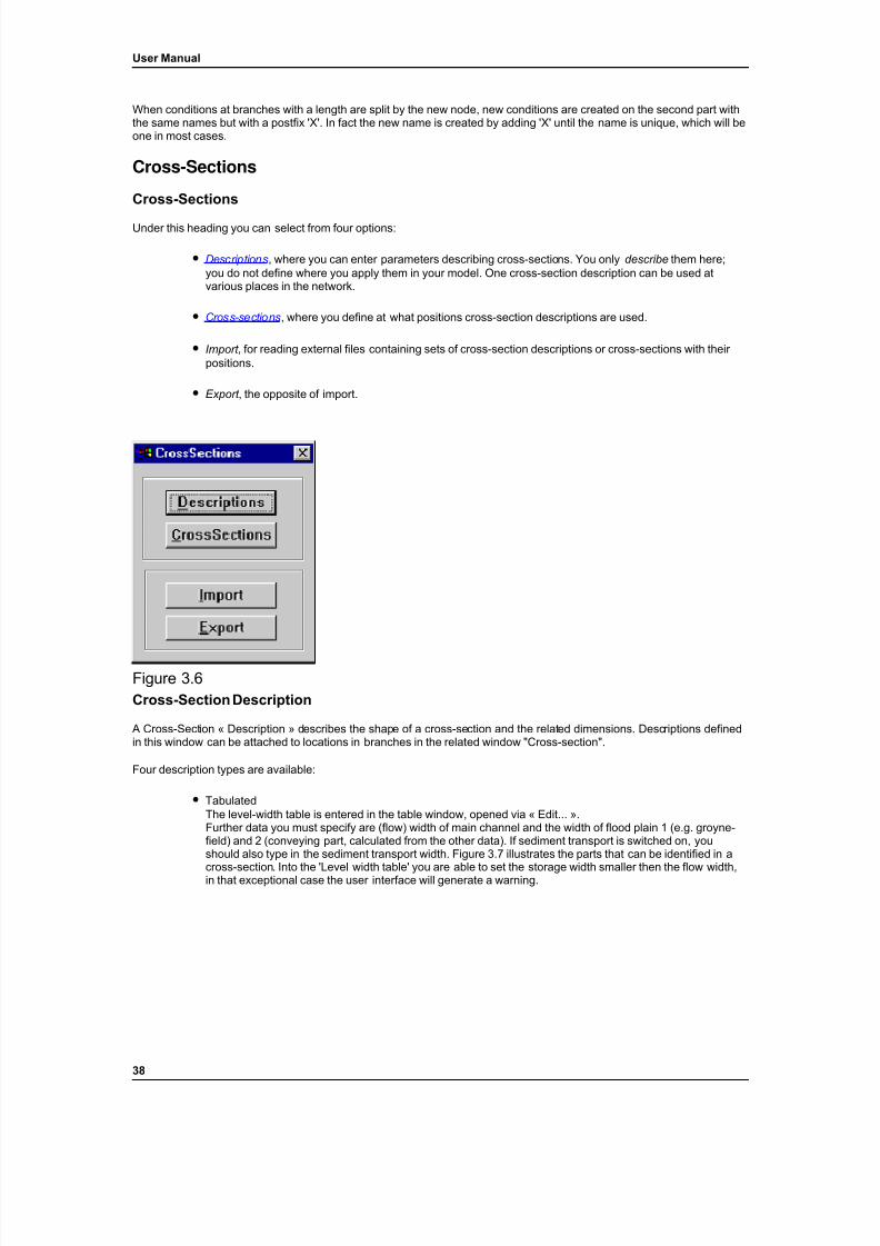
7/21/2019 SOBEK - UserManual
http://slidepdf.com/reader/full/sobek-usermanual 44/179
User Manual
When conditions at branches with a length are split by the new node, new conditions are created on the second part withthe same names but with a postfix 'X'. In fact the new name is created by adding 'X' until the name is unique, which will beone in most cases.
Cross-Sections
Cross-Sections
Under this heading you can select from four options:
• Descriptions , where you can enter parameters describing cross-sections. You only describe them here;you do not define where you apply them in your model. One cross-section description can be used atvarious places in the network.
• Cross-sections , where you define at what positions cross-section descriptions are used.
• Import , for reading external files containing sets of cross-section descriptions or cross-sections with their positions.
• Export , the opposite of import.
Figure 3.6Cross-Section Description
A Cross-Section « Description » describes the shape of a cross-section and the related dimensions. Descriptions definedin this window can be attached to locations in branches in the related window "Cross-section".
Four description types are available:
• TabulatedThe level-width table is entered in the table window, opened via « Edit... ».Further data you must specify are (flow) width of main channel and the width of flood plain 1 (e.g. groyne-field) and 2 (conveying part, calculated from the other data). If sediment transport is switched on, youshould also type in the sediment transport width. Figure 3.7 illustrates the parts that can be identified in across-section. Into the 'Level width table' you are able to set the storage width smaller then the flow width,in that exceptional case the user interface will generate a warning.
38

7/21/2019 SOBEK - UserManual
http://slidepdf.com/reader/full/sobek-usermanual 45/179
User Manual
Figure 3.7aWhen you chose the option ' Summer dike ' you can enter the information needed for the cross section of a river segment
with a summer dike WF , the dike crest level (m), the floodplain base level (m), the total and the flow area behindthe dike (m 2).
39
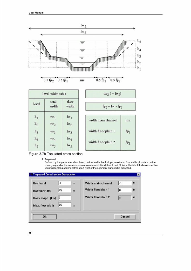
7/21/2019 SOBEK - UserManual
http://slidepdf.com/reader/full/sobek-usermanual 46/179
User Manual
Figure 3.7b Tabulated cross section• Trapezoid
Defined by the parameters bed level, bottom width, bank slope, maximum flow width, plus data on theconveying part of the cross-section (main channel, floodplain 1 and 2). As in the tabulated cross-sectionyou must enter a sediment transport width if the sediment transport is activated.
40
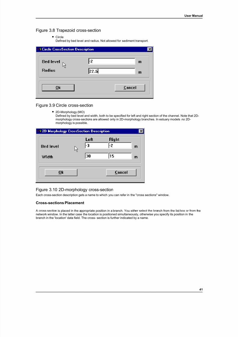
7/21/2019 SOBEK - UserManual
http://slidepdf.com/reader/full/sobek-usermanual 47/179
User Manual
Figure 3.8 Trapezoid cross-section• Circle
Defined by bed level and radius. Not allowed for sediment transport.
Figure 3.9 Circle cross-section• 2D-Morphology (MO)
Defined by bed level and width, both to be specified for left and right section of the channel. Note that 2D-morphology cross-sections are allowed only in 2D-morphology branches. In estuary models no 2D-morphology is possible.
Figure 3.10 2D-morphology cross-sectionEach cross-section description gets a name to which you can refer in the "cross sections" window.
Cross-sections Placement
A cross-section is placed in the appropriate position in a branch. You either select the branch from the list box or from thenetwork window. In the latter case the location is positioned simultaneously, otherwise you specify its position in thebranch in the 'location' data field. The cross- section is further indicated by a name.
41
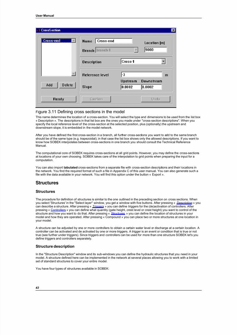
7/21/2019 SOBEK - UserManual
http://slidepdf.com/reader/full/sobek-usermanual 48/179
User Manual
Figure 3.11 Defining cross sections in the model
This name determines the location of a cross-section. You will select the type and dimensions to be used from the list box« Description ». The descriptions in that list box are the ones you made under "cross-section descriptions". When youspecify the local reference level of the cross-section at the selected position, plus (optionally) the upstream anddownstream slope, it is embedded in the model network.
After you have defined the first cross-section in a branch, all further cross-sections you want to add to the same branchshould be of the same type (e.g. trapezoidal); in that case the list box shows only the allowed descriptions. If you want toknow how SOBEK interpolates between cross-sections in one branch you should consult the Technical ReferenceManual.
The computational core of SOBEK requires cross-sections at all grid points. However, you may define the cross-sectionsat locations of your own choosing. SOBEK takes care of the interpolation to grid points when preparing the input for acomputation.
You can also import tabulated cross-sections from a separate file with cross-section descriptions and their locations inthe network. You find the required format of such a file in Appendix C of this user manual. You can also generate such a
file with the data available in your network. You will find this option under the button « Export ».
Structures
Structures
The procedure for definition of structures is similar to the one outlined in the preceding section on cross sections. Whenyou select 'Structures' in the "Select layer" window, you get a window with five buttons. After pressing « Description » youcan describe a structure. After pressing « Triggers » you can define triggers for the (de)activation of controllers. After pressing « Controllers » you can define what quantity (gate height, crest level or crest height) you want to control of thestructure and how you want to do that. After pressing « Structures » you can define the location of structures in your model and how they are operated. After pressing « Compound » you can place two or more structures at one location inyour model.
A structure can be adjusted by one or more controllers to obtain a certain water level or discharge at a certain location. Acontroller can be activated and de activated by one or more triggers. A trigger is an event or condition that is true or nottrue (see further under triggers). Since triggers and controllers can be used for more than one structure SOBEK let's youdefine triggers and controllers separately.
Structure description
In the "Structure Description" window and its sub-windows you can define the hydraulic structures that you need in your model. A structure defined here can be implemented in the network at several places allowing you to work with a limitedset of standard structures to cover your entire model.
You have four types of structures available in SOBEK:
42
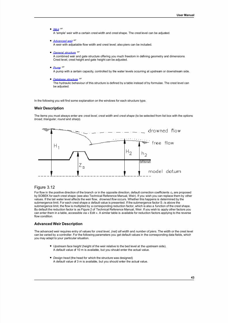
7/21/2019 SOBEK - UserManual
http://slidepdf.com/reader/full/sobek-usermanual 49/179
User Manual
• Weir WF
A 'simple' weir with a certain crest width and crest shape. The crest level can be adjusted.
• Advanced weir WF
A weir with adjustable flow width and crest level; also piers can be included.
• General structure WF
A combined weir and gate structure offering you much freedom in defining geometry and dimensions.Crest level, crest height and gate height can be adjusted.
• Pump WF
A pump with a certain capacity, controlled by the water levels occurring at upstream or downstream side.
• Database structure WF
The hydraulic behaviour of this structure is defined by a table instead of by formulae. The crest level canbe adjusted.
In the following you will find some explanation on the windows for each structure type.
Weir Description
The items you must always enter are crest level, crest width and crest shape (to be selected from list box with the options:broad, triangular, round and sharp ).
Figure 3.12For flow in the positive direction of the branch or in the opposite direction, default correction coefficients c w are proposedby SOBEK for each crest shape (see also Technical Reference Manual, Weir). If you wish you can replace them by other values. If the tail water level affects the weir flow, drowned flow occurs. Whether this happens is determined by thesubmergence limit. For each crest shape a default value is presented. If the submergence factor S f is above thesubmergence limit, the flow is multiplied by a corresponding reduction factor, which is also a function of the crest shape.By default the reduction factor is as Figure 2 of Technical Reference Manual, Weir. If you wish to apply other factors youcan enter them in a table, accessible via « Edit ». A similar table is available for reduction factors applying to the reverseflow condition.
Advanced Weir Description
The advanced weir requires entry of values for crest level , (net) sill width and number of piers . The width or the crest levelcan be varied by a controller. For the following parameters you get default values in the corresponding data fields, whichyou may adapt to your particular situation.
• Upstream face height (height of the weir relative to the bed level at the upstream side). A default value of 10 m is available, but you should enter the actual value.
• Design head (the head for which the structure was designed) A default value of 3 m is available, but you should enter the actual value.
43
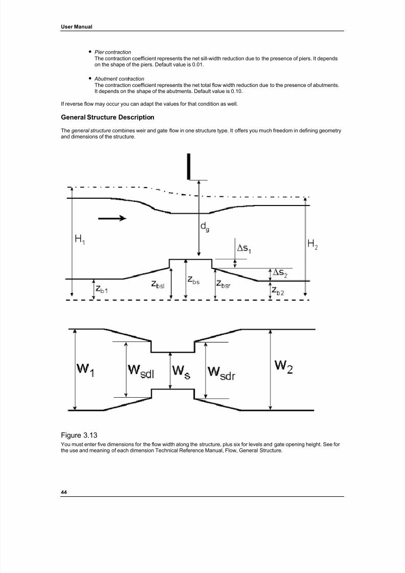
7/21/2019 SOBEK - UserManual
http://slidepdf.com/reader/full/sobek-usermanual 50/179
User Manual
• Pier contractionThe contraction coefficient represents the net sill-width reduction due to the presence of piers. It dependson the shape of the piers. Default value is 0.01.
• Abutment contractionThe contraction coefficient represents the net total flow width reduction due to the presence of abutments.It depends on the shape of the abutments. Default value is 0.10.
If reverse flow may occur you can adapt the values for that condition as well.
General Structure Description
The general structure combines weir and gate flow in one structure type. It offers you much freedom in defining geometryand dimensions of the structure.
Figure 3.13You must enter five dimensions for the flow width along the structure, plus six for levels and gate opening height. See for the use and meaning of each dimension Technical Reference Manual, Flow, General Structure.
44
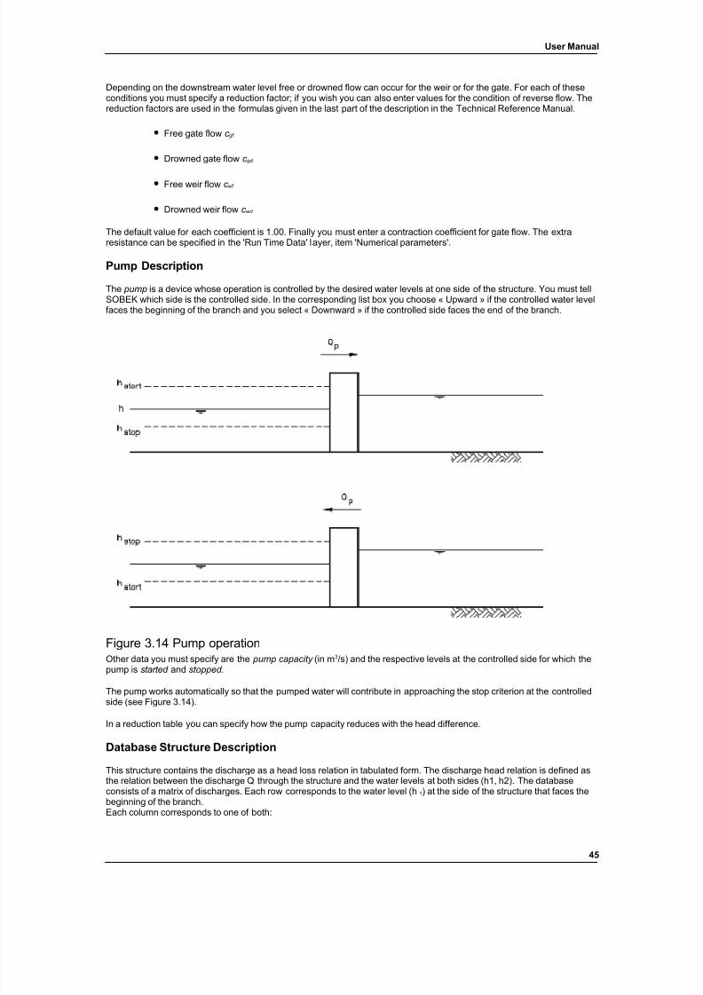
7/21/2019 SOBEK - UserManual
http://slidepdf.com/reader/full/sobek-usermanual 51/179
User Manual
Depending on the downstream water level free or drowned flow can occur for the weir or for the gate. For each of theseconditions you must specify a reduction factor; if you wish you can also enter values for the condition of reverse flow. Thereduction factors are used in the formulas given in the last part of the description in the Technical Reference Manual.
• Free gate flow c gf
• Drowned gate flow c gd
• Free weir flow c wf
• Drowned weir flow c wd
The default value for each coefficient is 1.00. Finally you must enter a contraction coefficient for gate flow. The extraresistance can be specified in the 'Run Time Data' layer, item 'Numerical parameters'.
Pump Description
The pump is a device whose operation is controlled by the desired water levels at one side of the structure. You must tellSOBEK which side is the controlled side. In the corresponding list box you choose « Upward » if the controlled water levelfaces the beginning of the branch and you select « Downward » if the controlled side faces the end of the branch.
Figure 3.14 Pump operationOther data you must specify are the pump capacity (in m 3/s) and the respective levels at the controlled side for which thepump is started and stopped .
The pump works automatically so that the pumped water will contribute in approaching the stop criterion at the controlledside (see Figure 3.14).
In a reduction table you can specify how the pump capacity reduces with the head difference.
Database Structure Description
This structure contains the discharge as a head loss relation in tabulated form. The discharge head relation is defined asthe relation between the discharge Q through the structure and the water levels at both sides (h1, h2). The databaseconsists of a matrix of discharges. Each row corresponds to the water level (h 1) at the side of the structure that faces thebeginning of the branch.Each column corresponds to one of both:
45
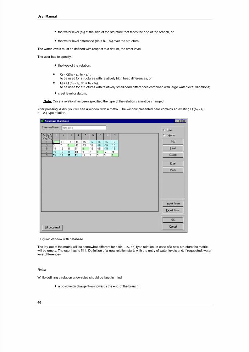
7/21/2019 SOBEK - UserManual
http://slidepdf.com/reader/full/sobek-usermanual 52/179
User Manual
• the water level (h 2) at the side of the structure that faces the end of the branch, or
• the water level difference (dh = h 1 h 2) over the structure.
The water levels must be defined with respect to a datum, the crest level.
The user has to specify:
• the type of the relation:
• Q = Q(h 1 - z s , h 2 - z s) ,to be used for structures with relatively high head differences, or
• Q = Q (h 1 - z s , dh = h 1 - h 2),to be used for structures with relatively small head differences combined with large water level variations;
• crest level or datum.
Note: Once a relation has been specified the type of the relation cannot be changed.
After pressing «Edit» you will see a window with a matrix. The window presented here contains an existing Q (h 1 - z s ,h 2 - z s) type relation.
Figure: Window with database
The lay-out of the matrix will be somewhat different for a f(h 1 - z s , dh) type relation. In case of a new structure the matrixwill be empty. The user has to fill it. Definition of a new relation starts with the entry of water levels and, if requested, water level differences.
Rules
While defining a relation a few rules should be kept in mind.
• a positive discharge flows towards the end of the branch;
46
7/21/2019 SOBEK - UserManual
http://slidepdf.com/reader/full/sobek-usermanual 53/179
User Manual
• a higher water level difference (h 1-h 2) should give a higher discharge;
• water levels and water level differences must increase if the row or column number increases;
• not all fields of the matrix need to be filled by the user. I.e. discharges corresponding to high headdifferences which will probably not be used in the computation can be omitted. These missing dischargeswill be generated by the program.;
• if during the simulation water levels occur that are outside the domain of the matrix (too high values)extrapolation will take place. At the end of the simulation messages will be given if at some time asolution was obtained outside the matrix;
• if the specified datum is a crest level the discharges in the matrix should be zero if the upstream water level is zero. A negative value (water level below crest) during simulation will result in a zero discharge;
• if the discharges in the matrix are not zero at zero upstream water levels or water level zero is not part of the matrix there is no crest level but just a datum. Then, in case water levels are too low to fit in the matrixduring simulation, extrapolation will take place.
Field color
• green fields indicate positions where the flow is supposed to be zero. This value will be insertedautomatically when adding/inserting a new row or column, on a position where h 1 - z s equals h 2 - z s or dhequals 0;
• blue fields indicate positions of values not specified by the user. These are generated automaticallywhenever the user clicks at «Fill Undefined» or «OK»;
• white fields are values specified by the user.
Edit buttons
After clicking at one of these buttons an action will be performed on either columns or rows, depending of the selected
radio button as follows:
• «Add», a number of rows or columns is added to the bottom/right of the matrix. Their title values (h 1 - z s ,h 2 - z s or dh) are asked for (and are checked for validity);
• «Insert», one row or column is inserted just before the current cell. If more than one cell (a block) wasselected, the function is canceled. The title value (h 1 - z s, h 2 - z s or dh) is asked for (and is checked for validity);
• «Delete», the row or column of the active cell is deleted; if more than one cell (a block) was selected, thefunction is canceled. If only two rows or columns are left, deletion is denied;
• «Copy», the data values (discharges, not the header value) of the row or column of the active cell arecopied to the Clipboard; if more than one cell (a block) was selected, that selection is copied to theClipboard. NB: Multiple rows or columns can be selected very easily by selecting the corresponding
header cells. The selection will automatically be downsized by excluding the header values;
• «Paste», the contents of the Clipboard is pasted into the selected data area of the matrix. If the contentsof the Clipboard does not fit the selected area, a warning message is displayed allowing the user to pasteanyway or cancel the operation. Pasting a smaller amount of data into the selected area will leave thebottom/right part of the selected area unchanged.
Import/Export buttons
47
7/21/2019 SOBEK - UserManual
http://slidepdf.com/reader/full/sobek-usermanual 54/179
User Manual
• «Export», at any time a matrix can be exported to an ASCII-text file;
• «Import», a matrix that was saved with the export command can be imported again.
Exported text files can be edited before importing as long as the structure of the file is not changed, i.e. the number of entries per row should be the same for each row (although the number of rows and columns can be changed). All enteredvalues should be valid real numbers. Note that ‘undefined’ values are represented by -9999.99 in this file.
Note: Only a valid matrix can be saved, but export can also be done for an invalid matrix. In contrast with saving,exporting cannot be cancelled.
OK/Cancel buttons
• clicking «Cancel» closes the matrix window and discards all changes made to this matrix;
• clicking «OK» results in checking the validity of the matrix. If the data is not found valid, an indicationabout the nature of the incorrectness will be displayed and control is returned to the user in order tocorrect the matrix. If the data is found valid the matrix is saved and the window is closed.
Special functions button
Depending on the type of the relation or state of the process of entering data some special functions are available. Thesefunctions can be selected by the appropriate button in the lower left corner of the window:
• «Check Grid», in case of a f(h 1 - z s , dh) relation validity checks will be performed.
In case of a f(h 1 - z s , h 2 - z s) relation there are two different functions available:
• «Copy h1 to h2», copy the header row values (h 1 - z s) to header column values (h 2 z s). This function willbe used when creating a new matrix only and will be available for as long as there are no data columnsdefined;
• «Fill undefined», replace the ‘undefined’ values in the matrix grid with calculated values (including validitychecks). This function will be available only if the matrix contains data.
Structure Placement
In the "Structure" window you can define in what branch(es), where and under what name you wish to apply a certainhydraulic structure. Either select the location in the ' Branch ' list box, with detailed co-ordinates entered in the ' Location 'field, or position with the mouse (right button), followed by « Confirm ».
A structure can not be placed on the node of a branch. Select one of the earlier described structures in the list box'Description '.
If and how a structure should be operated you can determine by clicking « Edit » in the Controller(s) box. You can thenselect up to four controllers from the list box containing the previously defined controllers.
When you take salt into account you will see a list box ' Salt concentration ' showing the following options (see for detailsand formulas Technical Reference Manual, Salinity Hydraulic structures):
• Equal The salt concentration is equal on both sides of the structure.
• SimpleVia « Edit... » you get a window where you can enter the upstream (' Left ') and downstream (' Right ') valueof the effective structure length ' Gamma ' (γ s).
• Complex Similar to the above option you enter the upstream (' Left ') and downstream (' Right ') value of the 'effective'structure length ' Gamma ' (γ s), plus the corresponding values for ' Gamma 1 ' (γ 1,l or r ) and ' Gamma 2 ' (γ 2,l or r ).
48
7/21/2019 SOBEK - UserManual
http://slidepdf.com/reader/full/sobek-usermanual 55/179
User Manual
Controllers
Controllers
Besides in this chapter the controllers are also more in detail described in Appendix G: Structure Control OptionsIncorporated in SOBEK River
A controller WF
is linked to a hydraulic structure. The action of the controller (which adjusts for instance a gate opening)has the aim to hold the water level or discharge at a specified location in the model on a user defined value. Of coursethat location should be within the direct control range of the structure. Some controllers can also set directly the controlledparameter of a structure (gate height) to user defined values.
Each controller can be switched on or off by a trigger WF .
In the main window "Structures" you can click the button « Edit... » in the box
Controller(s). Here you can select how many and which controllers you want to use. More than one controller can operateon the same hydraulic structure . However, a specific control parameter can be operated by just one controller at a time. ItI also possible to prescribe for instance the gate heights of a set of structures by only one controller if the heights areidentical.
In the window "Controller" you specify the following:
• Control updateThis defines how often the controller function should be updated. Normally this will be every time-step,but can also be an interval of more time steps. When you enter 1, the controller will be updated everytime-step; for 2 it will be updated every second time-step, and so on.For hydraulic controllers only, it is also allowed to specify a control update of zero. In that case thecontroller value will only be determined at the start of the active period and kept constant during the activeperiod (e.g. a half tide).Default is 1.
• Control parameter This parameter depends on the type of structure.
For pumps the operation is controlled by the start and stop level specified in the pump window.
For the weir, advanced weir and database structure the control parameter is the crest level.
For the general structure there is a choice of three parameters:
• crest level
• crest width
• gate height
Note: The discharge head relation which is schematised by the database of a database structure does not alter when the crest level changes. The user should be aware of this fact. However, in specific cases the deviations maybe relatively small.
• Parameter ‘dvalue/dt’ This parameter defines the maximum speed of increase or decrease of the control parameter. It providessome physical damping, to prevent that instabilities arise due to sudden changes in the structure opening.The parameter is only needed for controller types ‘Time’, ‘Relative Time’ and Relative from Value’. Withthe default 'dvalue/dt=0' the speed of opening or closing of a structure is unlimited (instantaneous). Withfor instance a value of ‘dvalue=0.1’, the speed of opening or closing of a gate is 0.1 m/s (e.g., 1 m changeof gate height in a computational time step of 10 s).
There are six controller types available for control of the structure parameters above:
• interval controller
• PID-controller
49
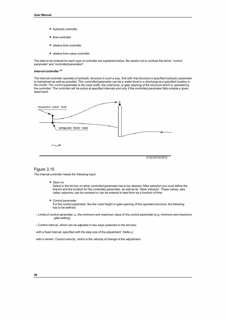
7/21/2019 SOBEK - UserManual
http://slidepdf.com/reader/full/sobek-usermanual 56/179
User Manual
• hydraulic controller
• time controller
• relative time controller
• relative from value controller
The data to be entered for each type of controller are explained below. Be careful not to confuse the terms ' control parameter' and ' controlled parameter'!
Interval controller WF
The interval controller operates a hydraulic structure in such a way, that with that structure a specified hydraulic parameter is maintained as well as possible. This controlled parameter can be a water-level or a discharge at a specified location inthe model. The control parameter is the crest width, the crest level, or gate opening of the structure which is operated bythe controller. The controller will be active at specified intervals and only if the controlled parameter falls outside a givendead band.
Figure 3.15The interval controller needs the following input:
• Steer onSelect in the list box on what controlled parameter has to be steered. After selection you must define thebranch and the location for the controlled parameter, as well as its ' Steer Value(s) '. These values, alsocalled setpoints , can be constant or can be entered in taed form as a function of time.
• Control parameter For the control parameter, like the crest height or gate opening of the operated structure, the followinghas to be defined:
– Limits of control parameter u s: the minimum and maximum value of the control parameter (e.g. minimum and maximumgate setting).
– Control interval, which can be adjusted in two ways (selected in the list box):
· with a fixed interval, specified with the step size of the adjustment ' Delta u s '
· with a certain ' Control velocity ', which is the velocity of change of the adjustment.
50
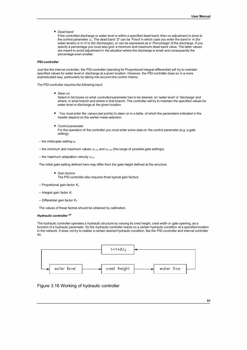
7/21/2019 SOBEK - UserManual
http://slidepdf.com/reader/full/sobek-usermanual 57/179
User Manual
• Dead band If the controlled discharge or water level is within a specified dead band, then no adjustment is done tothe control parameter u s . The dead band ' D' can be ' Fixed ' in which case you enter the band in m (for water-levels) or in m 3/s (for discharges), or can be expressed as a ' Percentage ' of the discharge. If youspecify a percentage you must also give a minimum and maximum dead band value. The latter valuesare meant to avoid adjustment in the situation where the discharge is small and consequently thepercentage even smaller.
PID-controller
Just like the interval controller, the PID-controller (standing for Proportional Integral differential) will try to maintainspecified values for water level or discharge at a given location. However, the PID-controller does so in a moresophisticated way, particularly by taking into account the control history.
The PID-controller requires the following input:
• Steer onSelect in list boxes on what controlled parameter has to be steered, on 'water level' or 'discharge' andwhere: in what branch and where in that branch. The controller will try to maintain the specified values for water level or discharge at the given location.
• You must enter the values (set points) to steer on in a table, of which the parameters indicated in theheader depend on the earlier made selection.
• Control parameter For the operation of the controller you must enter some data on the control parameter (e.g. a gatesetting):
– the initial gate setting u 0
– the minimum and maximum values u s min and u s max (the range of possible gate settings)
– the maximum adaptation velocity v max
The initial gate setting defined here may differ from the gate height defined at the structure.
• Gain factorsThe PID-controller also requires three typical gain factors:
– Proportional gain factor K p
– Integral gain factor K i
– Differential gain factor K d
The values of these factors should be obtained by calibration.
Hydraulic controller WF
The hydraulic controller operates a hydraulic structure by varying its crest height, crest width or gate opening, as afunction of a hydraulic parameter. So the hydraulic controller reacts on a certain hydraulic condition at a specified locationin the network. It does not try to realise a certain desired hydraulic condition, like the PID-controller and interval controller do.
Figure 3.16 Working of hydraulic controller
51
7/21/2019 SOBEK - UserManual
http://slidepdf.com/reader/full/sobek-usermanual 58/179
User Manual
Select the parameter that determines the operation of the structure, from the list box « Control Parameter ». The followingparameters can be selected:
• Water level Select a branch in the list box and define the location within that branch with the water level to be used for control of the structure.
• Velocity Select a branch in the list box and define the location within that branch with the flow velocity to be usedfor control of the structure.
• Flow directionSelect a branch in the list box and define the location within that branch with the flow direction to be usedfor control of the structure.
• DischargeHere you can select up to five branches in separate list boxes, with corresponding locations within thebranches. The total of the discharges of the branches is used for control of the structure.
• Head differenceSelect a structure in the list box of which the head difference is to be used for control of the structure. Theselected structure can be another one than the controlled structure!
• Pressure differenceSelect a structure in the li st box of which the pressure difference is to be used for control of the structure.The selected structure can be another one than the controlled structure!
The relation between the value of the hydraulic parameter (selected in this window) and the control parameter (of thecontrolled structure) is specified in tabulated form by editing in the « Control Table ». Header and number of columns areadapted to the selections made above.
The control parameter is, except in the case of a discharge, a function of the value of the hydraulic parameter at theprevious time step.
In case of discharge , the control parameter is a function of the discharge at the specified location(s) at a time , specifiedby the time lag , before the current time. A zero time lag means to use the discharge at the previous time step. Specifyingthe time lag for other parameters does not have any effect.
Time controller WF
Data for the time controller are entered in a table that pops up when you select ' Time ' in the main window "Controlparameters" under « Control type ». Using the time controller means that the crest level, gate setting or crest width is afunction of time, given in a tabulated form.
Relative time controller WF
The relative time controller can be used to specify the control parameter as a function of time, where the time (in seconds)is given relative to the moment that the controller is activated by a trigger. When the controller is turned on it starts at thetop of the table and continues downward until it is turned off by the trigger. When it reaches the end of the table the valueof the control parameter is kept constant at the last value.
The controller can start at the first value of the table over and over again. This will happen when the related triggers areactive again and the previous start was at least an amount of time ago specified by <<Start period>>.
Relative from value controller WF
The relative from value controller is also a time controller. It can be used when a control parameter has to be changed in agiven manner, but it is not known what value it will have when the controller is activated. Again the control parameter isspecified as a function of time, where the time (in seconds) is given relative to the moment that the controller is activatedby a trigger. When the controller is turned on it starts at the current value of the control parameter and continuesdownward until it is turned off by the trigger. When it reaches the end of the table the value of the control parameter iskept constant at the last value.
52

7/21/2019 SOBEK - UserManual
http://slidepdf.com/reader/full/sobek-usermanual 59/179
User Manual
The controller can start at the current value of the table over and over again. This will happen when the related triggersare active again and the previous start at the current value was at least an amount of time ago specified by « Startperiod ».
Note: A special point of consideration is the autostart option (Initial Conditions). At the start of the computationSOBEK will check for every structure if there is more than one controller active. A common error is that two time-controllers are defined; one for closing and one for opening a structure. In the timetable of these controllers adate/time is used lying somewhere before or at the start of the computation. To switch between these controllers,
triggers are used to make sure that only one controller is active. The problem arises when the autostart option isused, the state of the triggers i s not defined and SOBEK will detect two active time-controllers for one structureresulting in a error message. There is however a simple solution to this problem: use a relative time-controller instead of a normal time-controller. A relative time-controller is not active at the start of the computation, so noproblem occurs.
Triggers
A trigger determines whether a controller must be activated or de-activated, and can have the status ON or OFF. Under what conditions or at what events a trigger is ON or OFF is defined by a trigger parameter.
In the main window "Controllers" you can select how many and which triggers you want to use. If you have selected morethen one trigger the status of each trigger is an operand in a trigger expression. Then you have to specify the operator which can be OR or AND. The value or status of the trigger expression can be ON or OFF meaning active or deactive therelated trigger.
Up to four triggers can be part of a trigger expression. The expression will be evaluated according to the usual logicalrules. This means that AND has precedence above OR.
There are three types of trigger:
• Time trigger
• Hydraulic trigger
• Combined trigger (time and hydraulic)
Time trigger WF
The tresholds for switching of the status of a time trigger is defined in the trigger table . In the trigger table you can enter atime table and toggle in the right hand column between ON and OFF status by using the space bar.
Note: The trigger 'controls' the controller, rather than the hydraulic structure itself. When the trigger is ON, thecontroller comes into action.
Hydraulic trigger WF
The status of a hydraulic trigger depends on the value of either of the two following hydraulic parameters:
• the water level at a specified location
• the head difference over a specified hydraulic structure
• the discharge at a specified location
• the gate height of a specified structure
• the crest level of a specified structure
• the crest width of a specified structure
• the water level in retention area
• the pressure difference over a specified hydraulic structure
53
7/21/2019 SOBEK - UserManual
http://slidepdf.com/reader/full/sobek-usermanual 60/179
User Manual
What values are used as thresholds for the switch between ON and OFF is entered in the corresponding trigger table.You can toggle between > and < with the space bar. The operations > or < mean you check the criteria "larger than"threshold or "smaller than" threshold. This means you get criteria like: trigger is ON when the water level in branch i atlocation x is below y meter, otherwise trigger is OFF. If the gate height, crest level or crest width is chosen you can, instead of checking the ‘value’ against a threshold, also check if the value is increasing or decreasing (‘direction’).
The trigger table also contains a date/time column. This column gives the possibility to vary the trigger in time. The trigger is active from the first specified date/time. If the first given date/time is after the start of the simulation, the trigger will be
OFF until the specified date/time.
Note: To specify an Hydraulic Trigger which is constant for the complete simulation, just specify one row in whichthe date/time is equal or earlier than the start of the simulation.
Combined trigger WF
In the trigger table you specify values of threshold parameters for both time and a hydraulic parameter like water level or head difference. In the corresponding trigger table tou toggle the criteria and indicate whether you use the trigger in ANDor OR mode, meaning you want to check on either both criteria or at least on one. This allows criteria like trigger is ONwhen the water level in branch i at location x is below y meter AND the time is between 07:00 AM and 21:00 PM . If theoperator AND or OR remains constant the user can also define a combined trigger as a trigger expression of twooperands if he wishes.
Friction
Friction
Flowing water causes friction between the channel bed and the water. Often this effect causes (in rivers for sure) a veryimportant force acting on the flowing water. To simulate this force, you have to define bed roughness parameters.
On the water surface a wind shear stress can be accounted for (optional).
Bed friction WF
Bed roughness can be defined with one default value for the whole model with the « Model Wide » option. If the button isnot active then you must enter for each branch the roughness parameters (may be a function of place in each branch). If you want different values for some branches only, you can first define model-wide and then modify the few for which youwant different values. In other words, the «Model Wide» option sets the default roughness parameters for the currentmodel.
What parameters you must enter depends on the roughness formula you want to apply. Under «Friction Type» you find inthe list button the following options, each with the indicated parameters (see for exact formulas Technical ReferenceManual-WF).
• Chézy To be entered as a constant value (' Flow Coefficient ') or via « Edit... » as a taed function of water-level ,total discharge and/or place. If you did select water level par example and click <<edit>> an empty tablewith one column for the water level appears. Then you have to specify a location. This results in a extraempty column to be filled with Chézy values. The specification of another location results in a newcolumn, etc. The Chézy value in every grid point will be obtained by linear interpolation as a function of place and water level.
• Manning With the Manning coefficient nm a corresponding, to be entered as a constant or as a tabulated function of water-level , total discharge and/or place, Chézy value is calculated.
• Strickler KnWith the Nikuradse roughness coefficient k n a corresponding, to be entered as a constant or as atabulated function of water-level , total discharge and/or place, Chézy value is calculated.
• Strickler KsWith the Strickler coefficient k s a corresponding, to be entered as a constant or as a tabulated function of water-level , total discharge and/or place, Chézy value is calculated.
54
7/21/2019 SOBEK - UserManual
http://slidepdf.com/reader/full/sobek-usermanual 61/179
User Manual
• NikuradseVia the roughness coefficient k n a corresponding, to be entered as a constant or as a tabulated function of water-level , total discharge and/or place, Chézy value is calculated according to the White-Colebrookformula.
• Engelund The Chézy coefficient is calculated with the entered data on:'D90 Grain Size ', the grain size exceeded by 90 volume % of the grains'Global Engelund Parameters ', to be specified in a separate sub window via the parameters (for fullinformation see Technical Reference Manual-Flow: Roughness predictor):
• Delta D, the relative density of the bed material
• Theta Engelund
• Values for as 11 , as 21 , as 31 , as 12 , as 22 and as 32 which determine the Shields parameter of the occurring flowcondition.
For the flood-plain part of a cross-section you can specify separate roughness values. Furthermore you are able to set thebed friction for negative flow equal to positive flow or the bed friction for positive flow equal to negative flow (related to thebranch orientation). The same options can be applied for the flood plains.
Note: If the user has specified different tables for both flow directions and he makes the roughness of one directionequal to the roughness of the other direction by clicking at the appropriate button the previous defined table will be
overwritten.
Wind friction WF
Under this heading you specify wind friction coefficients and wind shielding factors. The wind data themselves (direction,speed) are in the layer ' Meteo data '. The geographical orientation of the channels is specified in the ' Branch ' windows.
The wind friction can be defined « Model Wide » or per branch, similar to the bed friction.
In the latter case you can take into account the effect of wind shielding . The default value for the wind shielding factor is 1,which stands for no shielding. There are two options:
• Constant over the whole branch.
• As a tabulated function of place
The "Global wind friction" window lets you define the other factors that are needed in the wind-shear stress formula: a 1, a 2
and ρ air (density of air).
Extra resistance
You can define local resistances ( head loss WF ) in addition to the loss caused by structures and bed and wind friction.Such a local resistance is defined by a dimensionless coefficient h, to be entered in tabulated form for each branch inwhich you want to include such a loss.
The parameter η figures in the momentum equation WF in the extra head loss term: g A f η or g A f ξ Q|Q| (with dimension m 3/s 2).
The head loss ∆h will effectively be ∆ h = η ∆ x or ∆ h = ξ Q|Q|
Note that the first option ( η) the head loss will depend on the local grid size ∆ x and for the second ( ξ) on the discharge.
Conditions
Conditions
Conditions can be seen as 'interface' between your model and the outside world. Conditions can be defined atboundaries, nodes and branches of the model. Depending on the physical aspects that are switched on in the "Model
Attributes" window, you can specify conditions for:
• Water flow
55
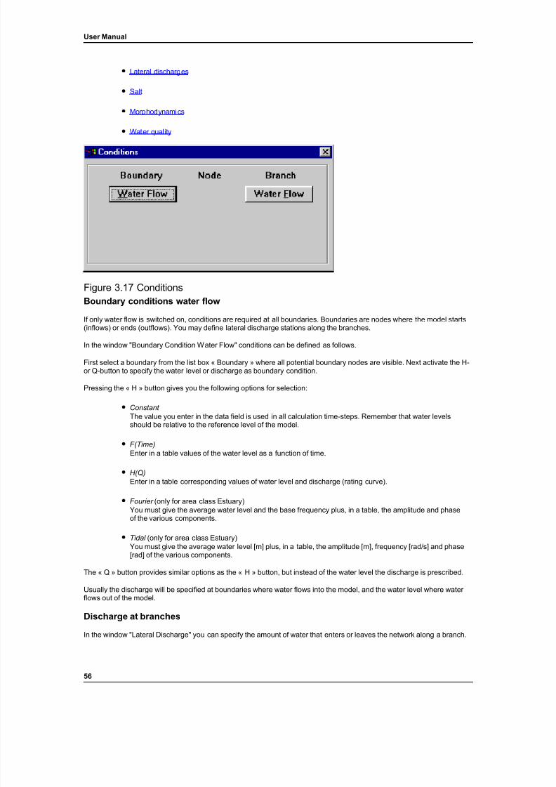
7/21/2019 SOBEK - UserManual
http://slidepdf.com/reader/full/sobek-usermanual 62/179
User Manual
• Lateral discharges
• Salt
• Morphodynamics
• Water quality
Figure 3.17 ConditionsBoundary conditions water flow
If only water flow is switched on, conditions are required at all boundaries. Boundaries are nodes where the model starts(inflows) or ends (outflows). You may define lateral discharge stations along the branches.
In the window "Boundary Condition Water Flow" conditions can be defined as follows.
First select a boundary from the list box « Boundary » where all potential boundary nodes are visible. Next activate the H-or Q-button to specify the water level or discharge as boundary condition.
Pressing the « H » button gives you the following options for selection:
• Constant The value you enter in the data field is used in all calculation time-steps. Remember that water levelsshould be relative to the reference level of the model.
• F(Time)Enter in a table values of the water level as a function of time.
• H(Q)Enter in a table corresponding values of water level and discharge (rating curve).
• Fourier (only for area class Estuary)You must give the average water level and the base frequency plus, in a table, the amplitude and phaseof the various components.
• Tidal (only for area class Estuary)You must give the average water level [m] plus, in a table, the amplitude [m], frequency [rad/s] and phase[rad] of the various components.
The « Q » button provides similar options as the « H » button, but instead of the water level the discharge is prescribed.
Usually the discharge will be specified at boundaries where water flows into the model, and the water level where water flows out of the model.
Discharge at branches
In the window "Lateral Discharge" you can specify the amount of water that enters or leaves the network along a branch.
56
7/21/2019 SOBEK - UserManual
http://slidepdf.com/reader/full/sobek-usermanual 63/179
User Manual
Under ' Specification ' you can define the type and magnitude of the lateral discharge. depending on the type you chooseyou get access to further data fields and list boxes
• Constant A constant in- or outflow (+ or –) can be entered, either as point source (in m 3/s) or as flow over a certainlength (in m 3/s/m 1). Length '0' implies a point source. Positive lateral discharge defines water entering themodel.
• F(Time)This option defines in tabulated form a lateral discharge as a function of time (point source (in m 3/s) or spread over a certain length (in m 3/s/m 1)).
• F(H)This option defines in tabulated form a lateral discharge as a function of the water- level at the (central)location of the lateral discharge (point source (in m 3/s) or spread over a certain length (in m 3/s/m 1)).
• StructureHere you can select a weir or general structure and specify a water level outside (with respect to themodel) the structure.
• Second StationYou can link a lateral discharge to another lateral discharge station. In that case a positive lateraldischarge at one station results in a negative lateral discharge of the same magnitude at the other station.This option transfers water from one location in your model to another.
• RetentionDefinition of lateral discharge from or to a retention area controlled by one or two structures.
Note: The discharge for a point source is given in m3/s and the discharge across a reach must be given inm3/s/m1.
Conditions salt
Conditions about the salt concentration can be specified for boundaries and at lateral discharge stations.
Salt at boundaries
See for full information the keyword Boundary conditions SA in the Technical Reference Manual, Salinity.
By pointing and clicking or by selecting in the list box ' Boundary ' (which shows all boundary nodes) you select a boundaryfor which you wish to enter salt conditions. In the list box ' Type ' you get two options:
• ConcentrationThe salt concentration (in kg/m 3) can be entered as a constant value or as a function of time in tabulatedform. The specified concentration will be used during inflow. In case of outflow an outflow condition will beused. For a (tidal) sea boundary in a model with Estuary as « Area class », where the water flow willalternately be out of and into the model, you can apply the Thatcher-Harleman time lag SA (in seconds).
• Zero Flux : representing a zero salt flux condition as, for instance, at a closed boundary.
Salt at branches
Salt can be discharged to the model at specified locations along branches. You must enter the following data:
• Name of the salt load.
• Branch on which the salt discharge takes place (selected from the list box) and the location in the branch(measured from the origin of the branch).
There are two options for the ' Type ' of load.
57
7/21/2019 SOBEK - UserManual
http://slidepdf.com/reader/full/sobek-usermanual 64/179
User Manual
• Dry load In this case the salt is discharged as powder or grains (mass). No water enters the system andconsequently the load does not figure in the water balance of the system. The salt can be dischargedover a certain length of the selected branch. For length '0' the discharge is a point load. You can enter thesalt load as a constant value or as a tabulated function of time.
• ConcentrationIf you select this option you get in the list box ' Lateral Discharge ' a list with lateral discharges that youdefined in the windows for water flow conditions. Here you can link a salt concentration ([kg/m 3]) to thelateral water flow. The salt concentration can be constant or a tabulated function of time. When water leaves the model, the local salt concentration in the model will be used.
Conditions sediment/morphology
The continuity equation MO for sediment requires a boundary condition at inflow boundaries. No conditions are required for outflow boundaries. Additional information is needed for nodes where three branches meet (confluences, bifurcations) andfor dredging and sediment supply. For each of these items you will find separate windows. They are described below.
Morphology at boundaries
For each inflow boundary (to be selected in the corresponding list box) you must specify one of the following items:
• Load
The sediment load at the inflow boundary can be specified in the following forms:
– Constant
– As a tabulated function of time
– As a tabulated function of the (water) inflow Q in the main section.
If you take into account quasi two-dimensional morphology you must enter values for the left and right part of the river cross-section.
• Bed level
The bed level at the inflow boundary can be specified as follows:
– Constant
– As a tabulated function of time
As with the load option you can specify values for the left and right parts of the cross-section if 2D-morphology isswitched on.
Morphology at nodes (with three or more branches)
As far as morphological aspects are concerned, bifurcations ST in a one-dimensional model are by definition problematic.Usually the sediment distribution over the outgoing branches is not directly governed by the water distribution, but rather by the local two- or three-dimensional flow pattern.
There are three options for the sediment distribution over the branch pairs that leave the node that you selected in the listbox:
• Proportional The sediment transport distribution is proportional to the water discharge distribution over the outflowingbranches.
• Linear The sediment transport distribution is a linear function of the water discharge distribution. The function isdefined by the coefficients a s and ß s , which can be entered in tabulated form.
58
7/21/2019 SOBEK - UserManual
http://slidepdf.com/reader/full/sobek-usermanual 65/179
User Manual
• RatioThe sediment transport and water distribution over a branch pair are expressed as ratios S 1 /S 2 and Q 1 /Q 2 .The relation between the ratios i s entered in tabulated form.
Remarks:
• The discharges used for the sediment distributions are the total discharges in the branch.
• The linear and ratio distribution method are only applicable in case of 2 outflowing branches.
Morphology at branches (dredging and sediment supply)
Sediment can be discharged to the model or taken out (dredged) at specified locations along branches. You must enter the following data:
• Name of the supply or dredging.
• Branch on which the supply or dredging takes place (to be selected in the list box) and the location in thebranch (measured from the origin of the branch).
There are two options for the ' Type ' of supply or dredging.
• Dry load In this case the sediment is discharged as mass only. No water enters the system and consequently theload does not figure in the water balance of the system.
• The sediment can be discharged or dredged over a certain length of the selected branch. For length '0'the discharge is a point load. The sediment load or dredging can be entered as a constant or as atabulated function of time.
• ConcentrationIf you select this option you get in the list box ' Lateral Discharge ' a list with lateral discharges (+ or –) thatyou defined in the windows for water flow conditions.
• Here you can link a sediment concentration to the lateral water flow. The concentration is entered as a
constant or as a tabulated function of time.
When you take 2D-morphology into account, you should provide under ' Section ' data for the left and right channel of across-section.
Conditions water quality
Under 'Conditions' you should specify the amount of pollutants entering the model area. At this point, the list of substances or state variables included in the water quality model, should already be defined. That can be done in the'Processes Library Configuration Tool' task. If the list of substances has not been defined yet, you will not be able to enter data for specific substances under Conditions.
You specify the amount of pollutants entering the model area in three ways:
• by defining the concentrations of the substances on the model boundaries;
• by defining the concentrations of the substances in the lateral discharges;
• by defining additional "dry" discharges of substances, outside of the modelled water balance.
The first two are only relevant for so-called "Active Substances": substances which are dissolved or suspended in thewater column and thus transported by the moving water. The last is also relevant for "Inactive Substances": substanceswhich are present in the sediment layer, and therefore NOT transported by the moving water.
59
7/21/2019 SOBEK - UserManual
http://slidepdf.com/reader/full/sobek-usermanual 66/179
User Manual
Water quality at boundaries
You specify the substance concentrations in the water entering the model area over flow boundaries in the window "Water Quality at Boundary Conditions". The water flow itself you must specify as a boundary condition in the similar windowunder « Water flow ».
The window asks for the following input:
• The boundary in question, to be selected from the list.
• The concentration per substance. You can select 'Constant' or 'F(time)', a tabulated function of time. For the time table option you will specify the times here. Enter the related substance concentrations under thenext option.
• For each active substance in the list shown you must specify a concentration. If the concentration variesin time you enter the values in a table. In the left column of that table you will find the times as entered inthe previous option.
Water quality flow at branches (!)
Under this heading you can optionally specify the concentrations of the substances in the lateral discharges. In addition tothe items already specified under « Water flow », you can specify here:
• The presence of substances in the lateral discharge in question, by ticking the corresponding tick box.Not ticking it means: all concentrations are zero. If you tick, you push the <Edit> button to proceed.
• The 'Waste Load Values' window allows you to enter active substance concentrations. If thecorresponding lateral discharge is time dependent, you have the option to make the concentrations timedependent as well.
Note that in this case the current version of Sobek does support distributed lateral discharges with an associated water quality substances load!
Water quality at branches
Under this heading you can specify "dry" waste loads (loads defined without a connection to the modelled water balance).Notice that these loads are specified as masses per time unit. In the window "Dry waste loads" you can specify thefollowing items:
• Name of the waste load.
• Branch in which the waste discharge is situated (to be selected in the list box) and the location in thebranch (measured from the origin of the branch).
• Section: the part of the cross-section in which the load is discharged (main channel, flood plain, .....)
• Length over which the load is discharged (for '0' you suppose a point load, the current version of Sobek does not support distributed dry loads, and thus neglects any number different from 0 ).
• Dry load function. You can select a constant value or a tabulated function of time. Here you can specify
the times for the time table option. Enter the related substance loads under the next options.
• Active substances. For each substance in the list shown you must enter a value in the corresponding datafield for the substance load.
• Non-active substances. Again, for each substance in the list shown you must enter a value in thecorresponding data field for the substance load.
Water quality conditions import options
You have two options to import the water quality conditions from a file on disk:
60
7/21/2019 SOBEK - UserManual
http://slidepdf.com/reader/full/sobek-usermanual 67/179
User Manual
• At the boundary/lateral discharge/dry waste load level you can use the <Import...> button to load a timeseries for all selected substances at once. The associated file format with headers is defined in AppendixC.
• At the level of individual substances you can use the <Load Table> button to load a time series for onesubstances at a time. The associated file format is the one without headers defined in Appendix C. Notethat the time points must be the same for all substances. For this reason, there is a separate form to editthem.
Initial Conditions
Initial conditions
Initial conditions define the starting situation for a calculation with SOBEK. Depending on the physical aspects you haveswitched on in the "Model Attributes" window you must specify initial conditions for:
• Water flow
• Salt
• Morphodynamics
• Water quality
First some general remarks on initial conditions. SOBEK will calculate the flows, sediment transport, etc, for thesubsequent time-steps of a simulation, while imposing the conditions specified in SOBEK's input windows under "Conditions". If you have perfect information on the initial conditions at your disposal, there will be no discrepancybetween the initial conditions and the actual situation at the beginning of the simulation. However, usually you will nothave such detailed information. In that case the model will need a number of time-steps for adaptation to the imposedconditions. The better the initial conditions fit into the conditions imposed on the first-time steps of the calculation, theshorter the adaptation period will be. This applies to the water flow computations as well as to salt, and water quality.
In the window "Initial conditions" you will see some special options for water flow and salt. Apart from « User Conditions »,which you specify for each physical aspect in data windows described below, you have the following option available:
Auto-startFor water flow this option lets SOBEK prepare itself a steady state condition at the begin time of the simulation
In each of the data windows described below you will find the option « Model Wide ». This option lets you defineparameter values that will be valid all over the model, unless you specify particular local values. So in this way you create'default ' values for the model.
Water flow
You can enter the initial water flow conditions in the model model-wide or per branch . Enter them in the form of discharges, and water depths or water levels (relative to model reference level).
Specify discharges and depths (or levels) as a constant or as a tabulated function of the location in a branch.
If you select « Model Wide » the initial conditions, specified discharge and water level (or water depth) will be used asinitial condition in all branches of the network. You may start for instance with flows at 0 m 3/s and all water depths at 1 m.However, you must realise that by entering values that are more plausible for the 'scale' of your model, you can drasticallyreduce the adaptation time.
Salt
You can enter the initial salt conditions in the model model-wide or per branch . For specification per branch (to select inthe list box) you can select under 'Type' for ' Salt ' or ' Chloride '. Either choice is then specified as constant concentration or as a concentration in a tabulated function of the location in the corresponding branch.
Morphodynamics
You enter the initial morphological conditions in the model model-wide or per branch . For specification per branch (toselect in the list box) you can select under 'Type' for constant parameters or a tabulated function of the location in thecorresponding branch.
61

7/21/2019 SOBEK - UserManual
http://slidepdf.com/reader/full/sobek-usermanual 68/179
User Manual
You enter the parameters in the form of characteristic sediment size, such as D35 , D50 , Dmedium and D90 . Which indicationsare needed depends on the transport formula that you apply to the entire model or to the considered branch (in the layer "Transport Formulas "). The window asks automatically for the correct data. If you did not yet select a transport formulayou get a likewise message. You may continue entering all asked grain size diameters.
What is not needed after the later selection of the transport formula will be neglected.
If 2D-morphology is accounted for, the characteristic diameters must be entered for the ' Left ' and ' Right ' channel.
Water quality
You can provide initial water quality conditions in the model in three ways:
• homogeneous initial conditions (" Model-Wide ");
• space dependent initial conditions;
• initial conditions from a restart file made in a previous simulation ( not supported by the current version ).
In the space dependent case you can define the initial conditions only at the branch level, but NOT at the WQ-segmentlevel, even if a branch contains more than one water quality segment.
At this point, the list of substances or state variables included in the water quality model, should already be defined. Thatcan be done in the 'Processes Library Configuration Tool' task. If the list of substances has not been defined yet, you willnot be able to enter data for specific substances under Initial Conditions.
To specify the initial conditions per branch you select a branch in the branch list. Via <Edit> you can provide data for "Active Substances" and "Inactive Substances". "Active Substances" are dissolved or suspended in the water column andthus transported by the moving water. You define initial conditions as a concentration (mass/volume). "InactiveSubstances" are present in the sediment layer, and therefore NOT transported by the moving water. In this case, youdefine initial conditions as a mass!! (This implies that the initial condition depends on the horizontal area of the segment,which is highly unpractical!)
Meteo Data
Meteo data
You can make the data specified under this heading valid « Model Wide » or valid per branch. For the data the following
categories are identified:
• Wind : direction in degrees (with wind blowing from the north = 0°, east = 90°, etc.) and velocity in m/s.
• Solar irradiance : expressed in W/m 2
• Water temperature : in °C.
You can specify all categories as a constant value or as a tabulated function of time.
Note: If you run the Water Quality module, you have to make sure that these meteorological parameters are indeeddefined. The program does not provide defaults, nor does it check whether or not those parameters have beendefined. If they are omitted, the water quality module will not work correctly!
Solar irradianceSolar irradiance plays a role in different types of water quality models:
• It is a driving force for the growth of algae, which typically use the irradiance inside the visual part of thespectrum (380-800 nm).
• It also determines the mortality of coliform bacteria. In that case, especially the ultra-violet range of thespectrum counts.
62
7/21/2019 SOBEK - UserManual
http://slidepdf.com/reader/full/sobek-usermanual 69/179
User Manual
Meteorological services often provide data for 'global i rradiance', which means all irradiance including the invisible parts of the spectrum in the infra-red and ultra-violet ranges. Make sure that you specify the right sort of irradiance data,depending on the water quality problem at hand. A typical conversion factor from 'global irradiance' to the visual spectrumirradiance is 0.45.
Dispersion
DispersionIf you have salt and/or water quality in your model you have to define a dispersion coefficient . There are four optionsavailable in SOBEK. They are listed in the main window "Dispersion".
• Option 1This option supposes a dispersion coefficient which is a function of place or time (or a constant)In the Water Quality model only this option is supported, and only as a constant (not a function in time or space).
• Option 2 This option supposes a linear dependency on the concentration gradient, specified by two functionsF1(x,t) and F2(x,t) , where (x,t) stands for a function of x or t .
• Thatcher-Harleman (only for salt application)This formula requires input of the following parameters: F1(x,t), F3(x,t) and F4(x,t) . All other requiredparameters are calculated by SOBEK itself, mainly from the water flow computation. Also here (x,t)stands for a function of x or t . See the Technical Reference Manual (Salinity) for full details.
• Empirical (only for salt application) An empirical dispersion formula based on the Thatcher-Harleman formula and requiring similar data asrequired there. See the Technical Reference Manual (Salinity) for full details.
In the list box « Type » you select whether the dispersion coefficient is constant, a function of time or a function of place.
In the sub-window "Dispersion coefficient" you enter the constant values of F1, F2, F3 and/or F4 , depending on theselected option and supposing you selected ' Constant ' in the list box « Type ».
If you did select ‘function of time’ and press << edit >> a table appears. Dependent on the selected option you have to fillF1, F2, etc in the table.
If you did select ‘function of place’ the sub window "Dispersion location" appears. Here you can define per branch aconstant or a table. Then you enter the values of F1, F2, F3 and/or F4, depending on the selected option and supposingyou selected ' Constant ' in the list box « Type ».
If you select in the main window « Thatcher-Harleman » or « Empirical » you get respective windows for:
• Fresh Water Discharge (only selection empirical)Defines a fresh water discharge in a branch (with a specified name and location in the branch), either positive (inflow) or negative (outflow).
• Mouth ParametersDepending on the selected dispersion formula, the following data are asked for all boundary nodes thatare part of an ' Estuary mouth ', the mouth to be selected in the list box « Mouth »:
– Reference water depth
– Reference salt concentration
– Characteristic flood velocity
– Seawater density ( ρ )
– Initial fresh water discharge
The following parameters are only required for the option dispersion type 'Empirical':
- P 0 , P 1, U 0 , U 1 (see Technical Reference Manual, Salinity)
63
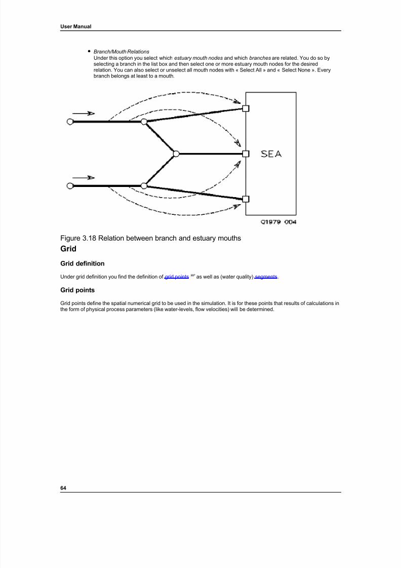
7/21/2019 SOBEK - UserManual
http://slidepdf.com/reader/full/sobek-usermanual 70/179
User Manual
• Branch/Mouth RelationsUnder this option you select which estuary mouth nodes and which branches are related. You do so byselecting a branch in the list box and then select one or more estuary mouth nodes for the desiredrelation. You can also select or unselect all mouth nodes with « Select All » and « Select None ». Everybranch belongs at least to a mouth.
Figure 3.18 Relation between branch and estuary mouths
Grid
Grid definition
Under grid definition you find the definition of grid points WF as well as (water quality) segments .
Grid points
Grid points define the spatial numerical grid to be used in the simulation. It is for these points that results of calculations inthe form of physical process parameters (like water-levels, flow velocities) will be determined.
64
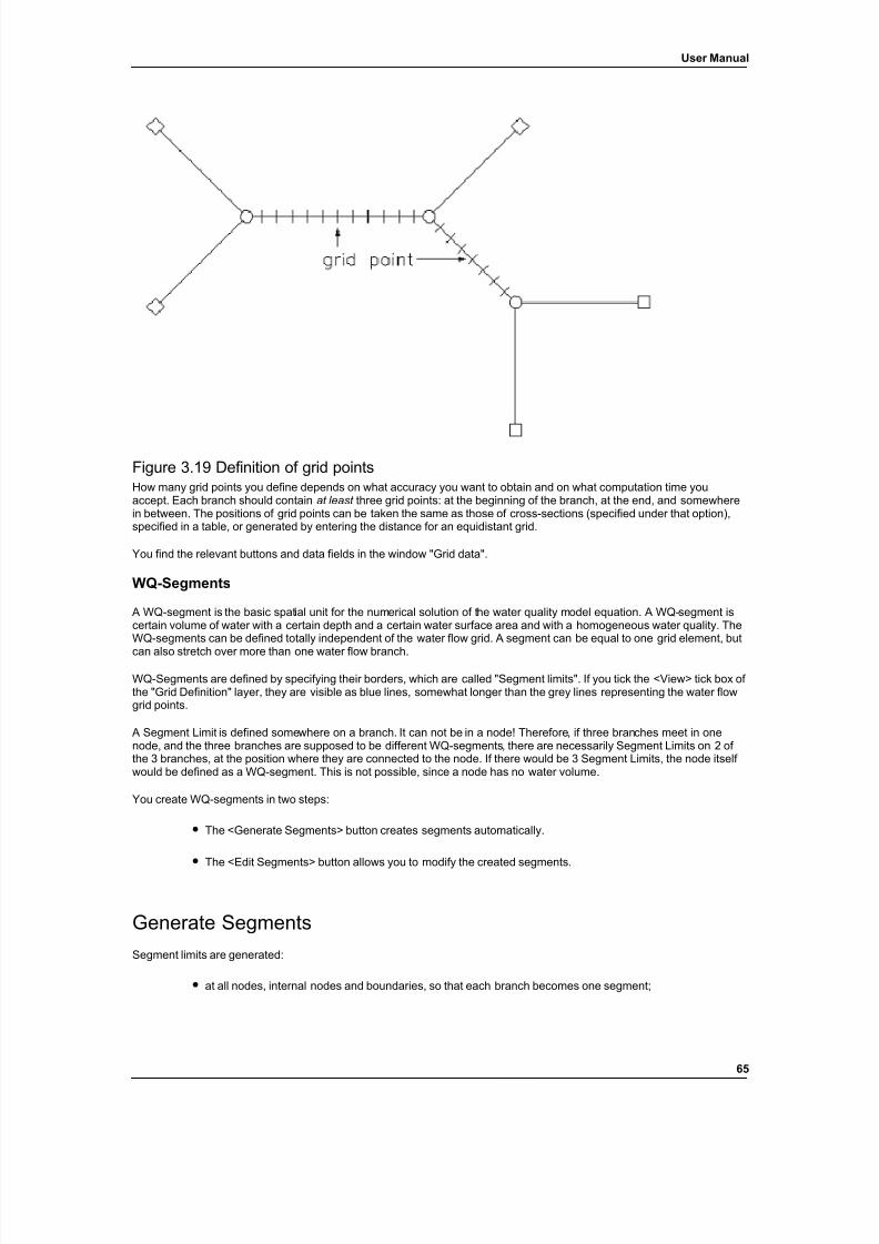
7/21/2019 SOBEK - UserManual
http://slidepdf.com/reader/full/sobek-usermanual 71/179
User Manual
Figure 3.19 Definition of grid pointsHow many grid points you define depends on what accuracy you want to obtain and on what computation time youaccept. Each branch should contain at least three grid points: at the beginning of the branch, at the end, and somewherein between. The positions of grid points can be taken the same as those of cross-sections (specified under that option),specified in a table, or generated by entering the distance for an equidistant grid.
You find the relevant buttons and data fields in the window "Grid data".
WQ-Segments
A WQ-segment is the basic spatial unit for the numerical solution of the water quality model equation. A WQ-segment iscertain volume of water with a certain depth and a certain water surface area and with a homogeneous water quality. TheWQ-segments can be defined totally independent of the water flow grid. A segment can be equal to one grid element, but
can also stretch over more than one water flow branch.
WQ-Segments are defined by specifying their borders, which are called "Segment limits". If you tick the <View> tick box of the "Grid Definition" layer, they are visible as blue lines, somewhat longer than the grey lines representing the water flowgrid points.
A Segment Limit is defined somewhere on a branch. It can not be in a node! Therefore, if three branches meet in onenode, and the three branches are supposed to be different WQ-segments, there are necessarily Segment Limits on 2 of the 3 branches, at the position where they are connected to the node. If there would be 3 Segment Limits, the node itself would be defined as a WQ-segment. This is not possible, since a node has no water volume.
You create WQ-segments in two steps:
• The <Generate Segments> button creates segments automatically.
• The <Edit Segments> button allows you to modify the created segments.
Generate SegmentsSegment limits are generated:
• at all nodes, internal nodes and boundaries, so that each branch becomes one segment;
65
7/21/2019 SOBEK - UserManual
http://slidepdf.com/reader/full/sobek-usermanual 72/179
User Manual
• at a lateral discharge, so that the segment on the branch is split in two parts upstream and downstream of the lateral discharge;
• at a structure, so that the segment on the branch is split in two parts upstream and downstream of thestructure.
Edit SegmentsBoth the windows "Limits" and "Segments" are used to edit the segments. They are strongly related and they pop upsimultaneously.
You can create additional segments by adding an additional limit, thus splitting an existing segment in two. You will see awindow popping up with fields to type names for the 2 new segments (indicated in red and blue in the model window). Thenew segments are added to the list 'Segments' in the window "Segments".
You can reduce the number of segments by deleting a segment limit, thus joining two existing segments in one. You willsee a window popping up which allows you to retain the name of one of the old segments for the new one. The removedsegment is deleted from the li st 'Segments' in the window "Segments".
You can move the position of a limit by clicking it and dragging it to its new position, or by typing the new position in theLimits window.
The fields 'Related segments' and 'State' in the window "Limits" keep you informed on what you have exactly defined. Youcannot change these fields yourself. The field 'State' can indicate 'Limit' (for 'normal' limits), 'Boundary' (a limit at aboundary node) or 'Redundant' (a limit that does not function as a separation between segments).
Note: Although the User Interface allows you to position segment limits anywhere in the network (and does soitself!) we advise you strongly to make the segment limits coincide with grid points from the hydrodynamic model. Inparticular, you have to make sure that you do not create 2 segment limits between the same 2 hydrodynamic gridpoints. This will surely cause the water quality model to crash.
Parallel segmentsTicking the tick box "Parallel Segments" makes the Water Quality module split the related segment in 3 parts: MainSection, Floodplain1 and Floodplain2 plus the storage part of the cross section. The names of the parallel segments areidentical to the mother segment name, with the last 4 characters replaced by "MAIN", "SUB1" and "SUB2".
Note: Lateral discharges and dry waste loads are always assumed to be positioned in the "MAIN" parallel segment.
Runtime Data
Introduction Run time data
Under run time data you specify matters like start and end time of the computation, time step size and some numericalparameters that have a specific influence on the calculation of flow, salt intrusion, morphology or water quality.
You also specify which parameters you want to be calculated by SOBEK.
In the main window "Run Time Data" there are buttons for the four main groups of data:
• Time parameters
• Numerical parameters
66
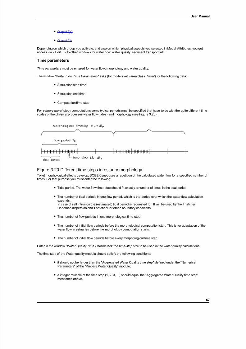
7/21/2019 SOBEK - UserManual
http://slidepdf.com/reader/full/sobek-usermanual 73/179
User Manual
• Output f(x)
• Output f(t)
Depending on which group you activate, and also on which physical aspects you selected in Model Attributes, you getaccess via « Edit... » to other windows for water flow, water quality, sediment transport, etc.
Time parametersTime parameters must be entered for water flow, morphology and water quality.
The window "Water Flow Time Parameters" asks (for models with area class ' River ') for the following data:
• Simulation start time
• Simulation end time
• Computation time-step
For estuary morphology computations some typical periods must be specified that have to do with the quite different timescales of the physical processes water flow (tides) and morphology (see Figure 3.20).
Figure 3.20 Different time steps in estuary morphologyTo let morphological effects develop, SOBEK supposes a repetition of the calculated water flow for a specified number of times. For that purpose you must enter the following:
• Tidal period. The water flow time-step should fit exactly a number of times in the tidal period.
• The number of tidal periods in one flow period, which is the period over which the water flow calculationexpands.In case of salt intrusion the (estimated) tidal period is requested for. It will be used by the Thatcher Harleman dispersion and Thatcher Harleman boundary conditions.
• The number of flow periods in one morphological time-step.
• The number of initial flow periods before the morphological computation start. This is for adaptation of thewater flow in estuaries before the morphology computation starts.
• The number of initial flow periods before every morphological time step.
Enter in the window "Water Quality Time Parameters" the time-step size to be used in the water quality calculations.
The time step of the Water quality module should satisfy the following conditions:
• it should not be larger than the "Aggregated Water Quality time step" defined under the "NumericalParameters" of the "Prepare Water Quality" module;
• a integer multiple of the time step (1, 2, 3, ...) should equal the "Aggregated Water Quality time step"mentioned above.
67
7/21/2019 SOBEK - UserManual
http://slidepdf.com/reader/full/sobek-usermanual 74/179
User Manual
Numerical parameters
In the window "Numerical Parameters for Water Flow" you can enter values for the parameters that SOBEK offers tocontrol the numerical computation of the water flow. Each parameter has a default value that is suitable for a wide rangeof applications. However, if a computation gives problems or when it is desired to decrease computation time, theadjustment of some of these parameters may be worthwhile. In the following we describe the use of the variousparameters.
• g: acceleration of gravity (9.81 m 2/s)
• Theta: weight factor used in the time discretisation of the Preissmann four-point scheme. The defaultvalue is 0.55, the minimum value is 0.5 (marginal stability), the maximum value 1.00 (which is in fact usedfor steady flow computations). Our advise is NOT to leave the default value too soon. Increasing the valueto 0.6 or 0.65 may in rare cases be necessary to provide the necessary dissipation for a successfulcomputation.
• Psi: weight factor used in the space discretisation of the Preissmann scheme. The default value is 0.5. ALWAYS USE THIS DEFAULT VALUE .
• Rho_w: density of fresh water (1000 kg/m 3)
• Pseudo Courant number recommended default: 0, this means automatic adaptation during simulation
(see TRM-WF
)
• Under relaxation parameter of the momentum equation: to maximise the convergence speed of flowcalculations, all terms of the SOBEK flow equations have been linearised. However, for a few coefficientslinearisation is not feasible. Underrelaxation is used instead, and the value of this parameter should be inthe range 0.2 - 0.5. A larger value (up to 0.9) may sometimes be possible, but will hardly improve theconvergence speed. On the other hand, a lower value is seldomly necessary, and is usually an indicationof an imperfection in the SOBEK schematisation. We recommend the use of a value of 0.3; for ̀ easy'problems a higher value may be possible, but for ̀ difficult' problems a lower value may be necessary, atthe expense of some loss of performance. Since it is not possible to give general guidelines of how todetermine the degree of complexity of a model, some experimentation with the value of the relaxationparameter is usually required.
• Under relaxation parameter for structures: relaxation of structure formulas is required because the appliedlinearisation may sometimes give rise to slightly incorrect solution updates, especially when the dischargethrough a structure is very small (this is inherent to the way that structures are modelled). The same rules
apply as for the relaxation parameter of the momentum equation, i.e., typical values are in the range 0.2 -0.5, depending on the degree of difficulty of the specified structure(s).
• Calculation mode: unsteady or steady flow.
• If no convergence on non-linearity: stop or continue . If after the maximum number of iteration steps stillno convergence has been achieved, by default the simulation stops. The user can choose to continue thesimulation. This can be useful if the truncation errors are only at a few time steps larger then the stopcriteria and yet relatively small. Inspect file 'Residu' in that case for the size of the truncation errors.
• Maximum number of iteration steps: in most cases the number of iteration steps needed will be less thanapproximately 10 (unsteady flow) or 50 (steady flow). Setting the maximum number of iteration steps at avalue of 100 (default) is therefore reasonable. However, for models with strongly varying cross-sectionsor when very small truncation criteria are specified, a higher value may be needed. When the flowcomputation has not converged to the given truncation criteria within the maximum number of iterationsteps (at each time step!), the computation terminates with a `no convergence' message.
• Stop Criterion for Nodal Administration Matrix: the Nodal Administration Matrix is solved by an iterativemethod (see TRM- WF). This iteration stops as soon as the truncation criterion is reached, the default valueis 10 -7. It is advised to leave this value unchanged. Taking a higher value will only marginally reduce thecomputational time, but may have a negative effect on the accuracy of the NAM solution. On the other hand, using a smaller value leads to insignificant increase of accuracy.
• Maximum number of iterations for Nodal Administration Matrix: the number of required iteration steps isusually limited to 25, so the maximum number can safely be set at a value of 50.
68
7/21/2019 SOBEK - UserManual
http://slidepdf.com/reader/full/sobek-usermanual 75/179
User Manual
• Stop criteria for variation in water level and discharge: for both the water level and the discharge atruncation criterion must be specified. Two aspects are of importance for the selection of proper values.Firstly, there should be a link with the accuracy you expect and require and secondly, you should keep inmind that the criteria must be small enough to avoid growing inaccuracies during the computation. Growthof inaccuracies may occur both in space and in time. For example, when you are doing a series of steady-state solutions, each new steady-state computation uses the previous steady-state solution asinitial condition. This initial guess may differ strongly from the steady-state solution that you want to obtainnext. Therefore, when at a certain moment the truncation criteria are satisfied at all grid points, there maybe a cumulative convergence error effect when the discharge and water level errors have the same signin (nearly) every grid point. As a result, the true convergence error may locally be O( N ) times larger thanthe specified truncation criteria, with N the largest number of grid points between any two boundarypoints.
• So this effect will especially be noticeable when your model consists of a number of consecutive branchesusing a total of several hundreds of grid points. Notice however that such a loss of accuracy occursmainly when the convergence speed is low, i.e., when a relatively low, fixed value of the Pseudo Courantnumber (see TRM- WF) is used. In unsteady calculations, (small) convergence errors are introduced eachtime step in the physical solution. Normally this does not pose any problem, since physical and numericaldissipation mechanisms take care of their damping. However, when too large truncation criteria are used,the accumulation of convergence errors may outweigh their dissipation, causing a larger and larger perturbation of the solution that finally leads to a break-down of the calculation. Again, this problem ismore likely to occur with very large models. It is easy to verify whether sufficiently small values for thetruncation criteria have been used. Simply rerun the calculation with values that are 2 to 5 times smaller,or higher. When the results of both calculations show no significant difference, then the largest set of
truncation criteria values was apparently small enough. It is in general a good idea to do this verificationfor at least one calculation out of a series of similar calculations.
• Extra resistance in general structure: default is zero.
• Numerical differentiation parameter for structures: because of the complexity of structure formulas,linearisation of structures is by means of numerical differentiation. A smaller value of the numericaldifferentiation parameter will therefore in crease the accuracy of this linearisation, up to the point thatcomputer round-off errors become significant. Safe values are in the range 0.001 - 0.00001; werecommend the use of the smallest value (i.e., 0.00001), which is the default (see also Numericalsolution WF). The same parameter is also used to smoothen the behaviour of general structures when thedischarge through such a structure is very small, as this could otherwise give rise to convergenceproblems. If you experience such problems, we advise you to use a higher value, up to 0.001 in order toavoid too much loss of accuracy.
•Transition height for summer dikes: the water level relative to the crest level of the summer dike at whichthe flood plain becomes completely filled up (see Summer dike WF)
The window "Numerical Parameters for Salt" asks for and ' Estuary length ' (in m). The above parameters are only askedfor area class ' Estuary '. The ' Estuary length ' is used only by the dispersion formulations 'Thatcher-Harleman' and'Empirical'.
The window "Numerical Parameters for Sediment" asks for the following parameters:
• Kinematic Viscosity : default is available for a temperature of about 20 °C: 1.00* 10 6 [m2/s]
• Relative density of the sediment, usually indicated by D. A normal value for sand is 1.65.
• Packing factor e = the pore fraction of the sediment, usually about 0.4. SOBEK computes the sedimenttransport inclusive of this pore volume.
• Alluvial layer factor a: determines a fictive layer with thickness d a , where the sediment transport "feels" anon-erodible layer. The layer thickness d a is a times the water depth (see Technical Reference Manual,Morphology, Fixed bed layer).
69
7/21/2019 SOBEK - UserManual
http://slidepdf.com/reader/full/sobek-usermanual 76/179
User Manual
• Reduction parameter for actual sediment transport width. The total sediment transport is obtained bymultiplying the actual transport width with the transport per unit width. If the actual flow width in thesimulation is less than the sediment transport width as given in the cross-section, the actual transportwidth will be the flow width multiplied by this reduction parameter.
The window "Numerical Parameters for Morphology" asks for the following.
Cross-sections can be modified in either « Equally over Transport Width » or « Proportional to Local Water Depth ».
You must further specify two parameters:
• Maximum number of time step reductions.
• Stability factor a c to prevent non-linear instability in the morphology computation. The default value is 1.01(see Technical Reference Manual, Morphology: Time integral).
The window "Numerical Parameters for Preparing Water Quality" asks for an ' Aggregation Time-Step Factor ', whichdetermines how many water flow time-steps should be aggregated to one "Aggregated Water Quality time-step".
The window "Numerical Parameters for Water Quality" provides a number of options to be used in the computation of thewater quality. See Technical Reference Manual, Water quality for details.
Main integration options
• Backward in space and time
• Modified 2nd order Runge Kutta
• 2nd order Lax Wendroff
• Alternating direction implicit
• Modified flux corrected transport
• Fully implicit integration
Sub integration options
• Use flows and dispersion as specified
• Use dispersion only if flow is not zero
• Use flows and dispersion as specified, but no dispersion over open boundaries
• Use dispersion only if flow is not zero, but no dispersion over open boundaries
• Use flow concentration transport over open boundaries
• Use higher order approximation of some numerical schemes
The sub-integration options are intended to allow the user to control:
• the automatic switching off of dispersion, if there is no advection (for those cases that the dispersionphenomenon is driven by advection);
• the automatic switching off of dispersion over open boundaries, to avoid the undesired influence of adownstream boundary condition on the solution;
70
7/21/2019 SOBEK - UserManual
http://slidepdf.com/reader/full/sobek-usermanual 77/179
User Manual
• the automatic adoption of an upwind spatial discretisation of the advection term over open boundaries, toavoid the undesired influence of a downstream boundary condition on the solution in numerical methodswhich use a central spatial discretisation of the advection term.
For further details, see " Introduction to water quality modelling with sobek " and " Transport Modelling and NumericalMethods ".
The window "Groundwater Numerical Parameters" asks for the following:
• Delta h : older water levels are discarded when the change in water level between two time steps is lessthen delta h
• Period Recent Water Levels : number of time steps for period of most recent water levels
• Period Less Recent Water Levels : number of time steps for period of less recent water levels
• Period Averaged Water Levels : in the period of less recent water levels all levels are averaged for thisnumber of time steps
• Period Older Water Levels : after the less recent water levels which are averaged, the older water levels
are checked with the delta h
• Period Initialisation : period after which groundwater calculation starts
Output f(x)
This option refers to the preparation of files containing the values of parameters as a function of place: per branch over aselected time stretch and for selected time intervals. For each physical aspect (water flow, salt, ...) there is a separatewindow where you can specify which parameters you want to be calculated and included in the output.
The common part of the windows is a sub-window in which you enter (see Figure 3.21):
• Report start time (date and time)
• Report end time (date and time)
• Report time step (frequency in number of time steps with which output is written to file).
Remember that the given times and time step for output may be different from those entered for the simulation. However,the output times should fall within the simulation period.
For each physical aspect you can activate options as listed below.
Water flow
Total Flow Main Flood Flood
Area Channel Plain 1 Plain2
Water level X
Discharge X X X X
Chezy coefficient X X X X
Area X X X X X
Width X X X X X
Average depth X X X X X
71
7/21/2019 SOBEK - UserManual
http://slidepdf.com/reader/full/sobek-usermanual 78/179
User Manual
Hydraulic radius X X X X
Average velocity X X X X
Froude number X
The various parts of the cross-section in the header of the table above refer to the following:
• Total : total cross-section, which may consist of a conveying part and a storage part.
• Flow area : the conveying part of the total cross-section, in which the following parts can be identified:
– Main channel
– Flood plain 1, e.g. the groyne-field part of the cross-section.
– Flood plain 2, e.g. the (conveying) floodplain part of the cross-section.
Besides the user selected parameters also the resulting maximum and minimum water levels during the simulation areincluded into the output.
Salt
Parameters that can be switched on for inclusion in the output are:
• Salt concentration
• Salinity
• Chloride concentration
• Density
• Dispersion coefficient
Sediment
Parameters that can be switched on for the output are:
• Sediment transport
• Dimensionless transport parameter
• Sediment transport in left channel (in case of 2D-morphology)
• Sediment transport in right channel (in case of 2D-morphology)
• Sediment transport exchange between left and right part of the river (in case of 2D-morphology)
Note :The selection of ‘Dimensionless transport parameter’ results in the output of two dimensionless parameters,namely the Shields parameter and the transport parameter.
Morphology
Parameters that can be switched on for the output are:
72
7/21/2019 SOBEK - UserManual
http://slidepdf.com/reader/full/sobek-usermanual 79/179
User Manual
• Bed level
• Increase of bed level with respect to start of run
• Mean bed level of main Channel
• Adapted cross-sections (according to the method in Technical Reference Manual, Morphology:Morphological changes of cross-sections)
• Increase of cross-sectional area (m 2) with respect to start of run
• Integrated sediment transport (integrated over time)
Water Quality
For water quality only the common window for entering start time and stop time plus time- step is shown.
The F(x) output will include all state variables but no extra output items . Consequently, extra items can not be selectedfrom a list box in the "Water Quality Map Reports" window.
Output f(t)
This option refers to output containing the values of specified variables as a function of time , for selected locations. For the active physical phenomena the same variables can be put in the output as can be done under the f(x) option;however, now as a function of time instead of location. The windows for each physical phenomenon show the sameselection opportunities as the f(x) output windows. You should specify a branch and location for output.
In addition reports can be made of the history of variables related to structures and lateral discharges .The output of lateral discharges is always in m 3/s, despite the fact that lateral input along a stretch is given in m 2/s.
For structures you can choose from a list for which structures you want a history report of discharge or an adjustableparameter (like e.g. gate openings).
Tidal analyses
Tidal analyses can be performed on some variables concerning flow and salt intrusion. Analysis of variables results in atable with characteristic values per variable for every tidal cycle. A characteristic value can be the maximum value within atidal cycle (high tide in case of water levels). For all characteristics that are calculated see TRM-WF.
Tidal analysis can be activated by selecting this option in the window where parameters can be selected for output as afunction of time. The user can select on which variables and at which places the analysis has to be performed. Flowmodule variables that can be analysed are:
• water level;
• discharge in total flow area, main channel or flood plains;
• average velocity in total flow area, main channel or flood plains.
On variables which are selected from this list to calculate output as a function of time, tidal analyses will be done if switched on. Analyses only takes place at the selected output locations.
Tidal analyses in the salt intrusion model will be done on the chloride concentration if that parameter is selected. If thisparameter is not selected but salinity or salt concentration, analyses will be performed on one of those parameters.
To be able to determine the start and end of every tidal cycle the user should specify an estimated tidal period. When tidalanalyses is switched on in either flow or salt module a pop up menu appears.
73
7/21/2019 SOBEK - UserManual
http://slidepdf.com/reader/full/sobek-usermanual 80/179
User Manual
Water Quality
The output locations are WQ-segments, to be selected from a list box in the "Water Quality History Reports" window.
The F(t) output will include all state variables plus extra output items . These extra items are no longer selected from a listbox in the "Water Quality History Reports" window. In stead, they are selected in the 'Processes Library ConfigurationTool' task.
Transport Formula
Transport formula
In the layer window you select 'Transport Formula' to tell SOBEK which sediment transport formula you want to apply ineach branch or model wide .
Next, in the corresponding "Transport Formula" window you select branches from the list
box, select the type of formula that you want to apply to the branch and add the branch to the list in the left sub-window.You have a choice from the following formulas:
• Engelund & Hansen
• Meyer-Peter & Müller
• Ackers & White
• Van Rijn
• Parker & Klingeman
• User-defined formula
You will find full details on these formulas in the Technical Reference Manual, section on sediment transport (ST).Parameters to be used in the transport formulas depend on local conditions and are derived by SOBEK from thecalculated water motion and also taken from the data windows specified under the « Morphodynamic » option in the layer 'Initial conditions' .
The user-defined formula is a general purpose transport formula. If you want to use the general formula you must define itby entering a number of parameters in the present window. They are indicated as Alpha_u, Beta_u, Gamma_u andTheta_c . The ripple factor can be supplied as a constant value or computed as done for the Meyer-Peter & Müller formula.The parameters can be adjusted in such a way, that the computed sediment transport matches your measured sedimenttransport.
The coefficients E1 to E7 refer to branches with 2D-morphology and should be calibrated for each model application with2D morphology. Default values are available.
Groundwater
Groundwater
In the "Groundwater Data" window you can define the groundwater parameters for the whole model with the << ModelWide >> option. If you want different values for some branches only, you can first define model-wide and then modify thefew for which you want different values. In other words , the << Model Wide >> option sets the default value for thegroundwater parameters for the current model.
You don’t have to supply groundwater parameters for the whole model area, branches for which you do not expect anyexchange with the aquifer can be left out. Of course you then must not use the model-wide option or set all values model-wide to zero.
When entering the parameters per branch, you can select a constant value for the whole branch, or enter a placedependent table.
74
7/21/2019 SOBEK - UserManual
http://slidepdf.com/reader/full/sobek-usermanual 81/179
User Manual
The parameters of the groundwater layer are:
• Storage coefficient : parameter to describe the capacity of the soil to carry water
• Hydraulic conductivity : indicator of the possible flow velocity through the aquifer
• Entrance resistance : parameter to describe the transport resistance of water from or to the aquifer.
• Initial groundwater level : the initial groundwater level in the aquifer
Making calculations
Making calculations
To make a calculation with SOBEK you select first 'Save' the model and then leave the Model Window with 'Exit'. Whenafter this the Schematisation Task is green and the Computation Task is yellow, the calculation can be started by clickingthe Computation Task.
During the computation first the PARSER will be executed in a DOS-Window. When the PARSER ends without any errorsSOBEKSIM will be started (also in a DOS-Window) to perform the actual calculations. During the calculation the progressis indicated by a progress bar.
Cutting and Combining of Schematisations
Introduction cutting and combining schematisations
Cutting and combining schematisations gives the ability to take parts of existing model schematisations and combinethem to a new schematisation. Of course it is also possible to connect two existing model schematisations without cuttingfirst.
After combining the concerning nodes have to be joined.
In 'How to cut a schematisation ' and ' How to combine schematisations ' all the necessary actions are explained.
How to cut a schematisation
Cutting is done from the active case:
• Open the case from which you want to select and cut a piece.
• Start the task block ‘Schematisation’
• In the SOBEK-Model Window select the menu i tem‘Operations’ -> ‘Select Schematisation’.
• Using ‘Start Polygon’, and by clicking points, and the ‘Finish Polygon’ button you can draw a polygon(maybe very complex). In between you are allowed to zoom in, but you are not allowed to edit a datalayer.
• The selected nodes inside the polygon will turn green.
• By clicking on the nodes, using the right mouse button you can see the name of the node in the list whilethe node is turn red. By clicking the left mouse button in the list with node names the node with theselected name is turned red. To remove the red node indication click with the right mouse button in emptyspace of the Model Window.
• Using the ‘Store selected nodes’ button the list of selected nodes is saved. You will be reminded to 'Save'the model before leaving the schematisation.
• If you are not satisfied and want to change the selection, just do it again; each time you save the list of selected nodes, the file containing the selected nodes is overwritten.
75
7/21/2019 SOBEK - UserManual
http://slidepdf.com/reader/full/sobek-usermanual 82/179
User Manual
• Save the model (Is necessary for the CMT to perform ok afterwards!)
• Exit the Schematisation and return into the CMT
• Use the Right mouse button to click on the Schematisation block and select ‘Cut Schematisation’ in thepop up menu
• Now it is checked if all the necessary files are available in the right place. If not you will get a message.When all the files are found the cutting will be performed and you will get a message when it is finished.
• To check the cutting messages use the Right mouse button to click on the Schematisation block andselect ‘Show Cut Messages’ in the pop up menu
• Use ‘Save as’ to save the case under a new name
• Continue working with the new case, and making the cut schematisation correct. You will certainly needto validate the model again, since cutting may have introduced new boundaries in the schematisation.You can also use the new schematisation in combining it with other schematisations.
How to combine two schematisations
Combining is done by adding a selected schematisation to the active case:
• Open the case or create a new case with 'Open As New' which contains the schematisation you want tocombine with another
• Go into the task block ‘Schematisation’, Save the model and Exit. This necessary for the CMT toperform ok afterwards.
• Use the Right mouse button to click on the Schematisation block and select ‘Combine Schematisation’ inthe pop up menu. If you did not save the model as described above you will get a warning with therequest to do so.
• Select the case you want to add to the active case.
• Specify a (dx, dy, dz) shift for the selected schematisation to be added. Default is (0,0,0), but the co-ordinate system of the two schematisations could be different. The co-ordinates of nodes (dx,dy) in theadded schematisation are shifted with dx and dy. The vertical shift (dz) is only applied in Initial water level(constant only) and Cross-sections.
• All SOBEK data objects in the added schematisation will get the prefix 'P_' before their original names.
• To check the messages use the Right mouse button to click on the Schematisation block and select‘Show Combine Messages’ in the pop up menu.
Note: Model wide definitions/settings of the 'receiving' prevail over model wide definitions/settings of the 'adapted'model.
Continue working with the new case, and making the newly created schematisation correct. You will definitely need to joinnodes to connect the two parts together and validate the model again.
If desired the prefixes can be removed with Operations->Remove Prefix menu option in the SOBEK Model Window .
Application of Sobek
General
SOBEK is typically used for studying a wide range of subjects related to water channel systems.
The physical phenomena are modelled in one dimension (along the river or channel axis), giving the user insight into thecross-sectional average value of several parameters in the water system.
76

7/21/2019 SOBEK - UserManual
http://slidepdf.com/reader/full/sobek-usermanual 83/179
User Manual
To give some idea of the wide range of SOBEK applications, in the following sub-sections some specific subjects aredescribed, in which SOBEK can play a role.
The given applications are examples only, not restricting the use for other related subjects.
In the last sub-sections the major limitations of the SOBEK system are described. For a more formal description of theSOBEK limitations we refer to the SOBEK validation document. This document will be sent to you upon request.
River trainingRiver training are measures imposed by man to change the behaviour of a river or river system. Typical river trainingmeasures can be: embankments, groynes, reducing or increasing the river width, hydraulic structures. By applying river training works, we try to force the river to behave more according to our preferences.
The SOBEK system can be used to study the effect of proposed river training works on the river and allows the user tooptimise the design of the river training.
The following SOBEK modules can be used to study the indicated effects:
flow module water levels, flow velocities, inundation time and frequencies, discharge distribution over the channel network
sediment transport module initial aggradation and degradation
morphology module long-term morphodynamic effects: changes of bed levels, water levels and discharge distribution
River canalisation is the extreme form of river training: the river is forced into a sharply defined behaviour. The use of SOBEK in river canalisation studies is the same as for river training.
Dredging optimization
Dredging is an expensive method to make or keep a river navigable. It is worthwhile to keep the amount of material to bedredged as small as possible, and to reduce the necessary dredging frequency to an absolute minimum.
One-dimensional modelling systems are excellent tools to prepare and optimize a dredging schedule for a river reach or channel network. When you know the requirements for the least water depth, the best dredging scheme with respect tocosts and effect can be selected.
The following SOBEK modules can be used to study the indicated effects:
flow module water depths, flow velocities
sediment transport module indication of aggradation and degradation reaches
morphology module in combination with the flow module: water depths in relation to proposed dredging activities.
Water quality
The quality of water is of major importance for various rea sons: the water may be used for drinking purposes; ecology(biological diversity); aesthetics (a strongly polluted river may look and smell quite unpleasant); reasons of a judicialnature, and so on.
Therefore, water quality simulations are carried out so as to predict the effects of accidental spills, to determine the criteriafor discharge permits, to verify whether companies and other organisations along the river behave correctly.
The following SOBEK modules can be used to study the indicated effects:
flow module water depths, flow velocities, discharges to be used as input for the water quality simulation
water quality module concentrations of modelled substances, balances of various substances
River bend cut-offs
Many of the low-land rivers show a meandering channel pattern. There may be reason to reduce the total length of a river by removing meander loops: reduction of the navigation length between two locations, reduction of the amount of river training works, increase of the discharge capacity for flood relief and so on.
77
7/21/2019 SOBEK - UserManual
http://slidepdf.com/reader/full/sobek-usermanual 84/179
User Manual
As these bend cut-offs may have a direct serious effect, or worse, an effect in the long run, they should be studiedthoroughly before they are actually constructed.
The following SOBEK modules can be used to study the indicated effects:
flow module water levels and depths, flow velocities
sediment transport module indication of aggradation and degradation reaches
morphology module in combination with the flow module: water levels and depths, in particular upstream of the bend cut-off.
Water flow
You can enter the initial water flow conditions in the model model-wide or per branch . Enter them in the form of discharges, and water depths or water levels (relative to model reference level).
Specify discharges and depths (or levels) as a constant or as a tabulated function of the location in a branch.
If you select « Model Wide » the initial conditions, specified discharge and water level (or water depth) will be used asinitial condition in all branches of the network. You may start for instance with flows at 0 m 3/s and all water depths at 1 m.However, you must realise that by entering values that are more plausible for the 'scale' of your model, you can drasticallyreduce the adaptation time.
Regime changes
The regime (long-term discharge distribution in the river system over a hydrological year) of a river may change in thecourse of time. This change can be the result of natural causes, such as climatological changes or the result of humaninterference, such as reservoir operation.
In the case of climatological changes, various scenarios can be easily simulated using SOBEK to study future changes inthe river regime. In the case of reservoirs, various operation strategies can be simulated to optimise the reservoir operation.
The following SOBEK modules can be used to study the indicated effects:
flow module future water levels and discharges
water quality module water quality as a consequence of the regime changes
morphology module long-term bed-level changes, effect of sediment-transport block age caused by the reservoir.
Flood risk
One-dimensional modelling systems are very suitable for computing accurate water-level predictions in rivers. This makesthese systems excellent tools in flood-risk studies.
Present flooding risks can be estimated by carrying out computations with a calibrated model under the presentconditions. Further, the effect of flood-risk mitigating measures can be assessed.
The following SOBEK modules can be used to study the indicated effects:
flow module flooding frequency analysis, maximum water level prediction
sediment transport module sediment-transport prediction during high discharge
morphology module long-term bed-level changes (and their effect on the water levels).
Low water
Comparable to the flood-level studies are low-water studies. Low-water studies are particularly important for navigationand for water-intake structures.
Overall design of the navigation channel, and determination of the design level of an intake structure can be carried outwith the SOBEK system.
78

7/21/2019 SOBEK - UserManual
http://slidepdf.com/reader/full/sobek-usermanual 85/179
User Manual
The following SOBEK modules can be used to study the indicated effects:
flow module least available depth and water level at locations and along reaches, available discharge
morphology module life-time of the designed navigation channel, future water levels in the water intake.
Major limitations
One-dimensional
SOBEK is a one-dimensional modelling system. This implies, that problems in which two- and three dimensional floweffects are of importance, the application of SOBEK is not without risk. In particular if the subject of the study is directlygoverned by those multi-dimension al effects.
In fact, most of the other major limitations follow from the assumptions made for a one dimensional approach.
example
the distribution of non-cohesive sediment transport at river bifurcations is strongly governed by the local two- and threedimensional flow pattern. This makes a one dimensional modelling approach unsuitable to study measures to change thissediment transport distribution. On the other hand, this does not imply that it is impossible to make a one dimensionalmorphological model with bifurcations.
end of example
Horizontal water surface
The water level in a cross section is horizontal in the direction perpendicular to the channel axis. This means that in verywide channels or flood plains errors may be introduced. In particular the filling and emptying process of a modelled floodplain may become unrealistic.
Sub-critical flow
SOBEK has been designed to give optimal performance and reliability for sub-critical flow conditions, which means aFroude number smaller than 1 (one).
In case the Froude number exceeds 1 during computation this computation will terminate.
A module for super-critical flow for SOBEK is envisaged for the near future.
Tutorial
General
With the tutorial in this Section we will take you by the hand and guide you through various SOBEK options and facilities.However, the tutorial will not show you everything. That would be an impossible task because of the enormous range of options, selections and other possibilities.
Let us see what this tutorial has in stock for you:
1. the setting up of a model consisting of two branches
2. expansion of this model to three branches
3. boundary conditions (constant conditions and time functions)
4. lateral inflow
5. hydraulic structure
6. alluvial roughness
7. run time data
8. the creation of results and how to present them in tables and diagrams
79

7/21/2019 SOBEK - UserManual
http://slidepdf.com/reader/full/sobek-usermanual 86/179
User Manual
The tutorial will also not explain all options in all windows appearing during a session. Once you get the hang-and-feel of the system, you may wish to browse through the options not dealt with in the tutorial. To make sure the tutorial will lead toa successful computation, we advise you to stick to the procedure as described.
Setting up of the model
We consider a main canal in an irrigation network. The canal has a simple trapezoidal cross-section profile, see Figures5.1 and 5.2.
Figure 5.1 Layout of model
We will schematise the reach as two branches joining in a node. A reach like this may also be modelled as one branch,but as we like to extend the model with a third branch in a later stage, it is more convenient to define a node at thelocation we want to connect to this third branch.
Suppose we want to model a reach of 20km. Then we can enter the following data:
Length of branch 1: 10000 m
Length of branch 2: 10000 m
Bed level slope: 2 10 -4
A positive slope means lower bed level in positive x-direction.
The cross-section has the profile as given in Figure 5.2.
Figure 5.2 Cross-sectional profile at node 'node2'
This is a simple trapezoidal profile with a bank slope 1:3. The bed level at the node is –3.00 m (with respect to thehorizontal reference plane).
There are sufficient data to enter as the required input for the data layers 'topography' and 'cross-sections' of the "SelectLayer" window in the SOBEK user interface.
• start up the SOBEK system
80

7/21/2019 SOBEK - UserManual
http://slidepdf.com/reader/full/sobek-usermanual 87/179
User Manual
• select 'Create Project'
• enter the project name: MYTUTOR
• answer question 'Do you want....' with 'Yes'
• Now you are in the Case Management Tool (CMT). Select 'Case' -> 'Open as new'
• Enter name of new case: My Tutorial Model and click 'OK'.
• Double click on 'Model Schematisation'
Three new windows pop up: the "SOBEK-model" window, the "Select Layer" window and the "Messages" window.
At first we have to, deal with the "Model Attributes" window. Here you select the area class, the physical processes to bemodelled, and you enter the overall size of the area to be modelled. See Model Attributes for more information.
• Open the Model Attributes window by selecting 'File' -> 'Model Attributes' in the Model window.
• Select area class 'Estuary' : point at the corresponding radio button with the mouse pointer and press(click) the left mouse button.
• Activate physical aspect 'Water Flow': point at the corresponding push button with the mouse pointer andpress (click) the left mouse button. (Probably the water flow option is already switched on by default whenthe window appears)
Do NOT , at this stage, activate any other physical aspect!
Set the limits of the geographical area:
• Enter 0 for the 'X Minimum' data field, 22,000 for the 'X Maximum' data field, 0 for the 'Y Minimum' datafield and 22,000 for the 'Y Maximum' field.
• You select a data field for editing by pointing at it with the mouse pointer and clicking the left button.Double clicking will bring you in override mode.
Before leaving the "Model attributes" window, make sure it looks like Figure 5.3.
81
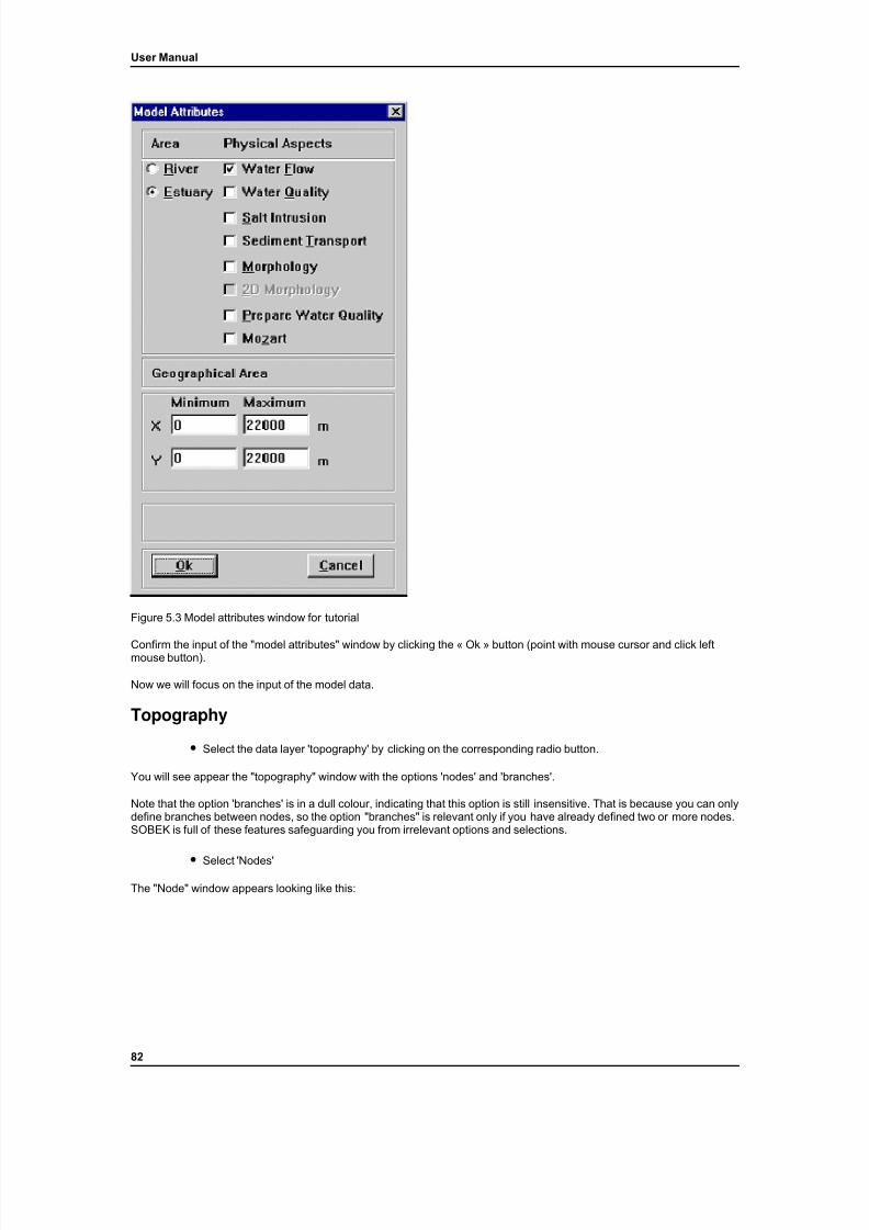
7/21/2019 SOBEK - UserManual
http://slidepdf.com/reader/full/sobek-usermanual 88/179
User Manual
Figure 5.3 Model attributes window for tutorial
Confirm the input of the "model attributes" window by clicking the « Ok » button (point with mouse cursor and click leftmouse button).
Now we will focus on the input of the model data.
Topography
• Select the data layer 'topography' by clicking on the corresponding radio button.
You will see appear the "topography" window with the options 'nodes' and 'branches'.
Note that the option 'branches' is in a dull colour, indicating that this option is still insensitive. That is because you can onlydefine branches between nodes, so the option "branches" is relevant only if you have already defined two or more nodes.SOBEK is full of these features safeguarding you from irrelevant options and selections.
• Select 'Nodes'
The "Node" window appears looking like this:
82
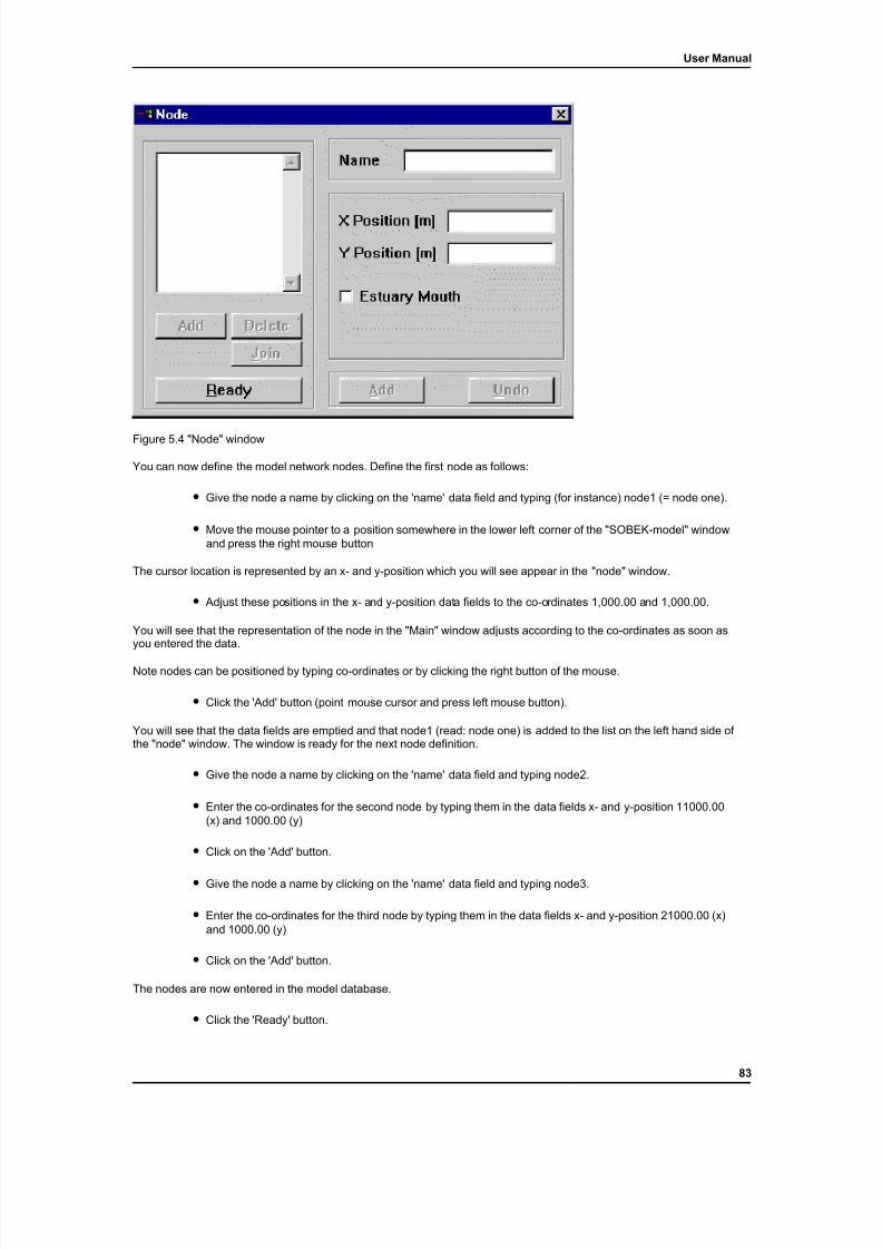
7/21/2019 SOBEK - UserManual
http://slidepdf.com/reader/full/sobek-usermanual 89/179
User Manual
Figure 5.4 "Node" window
You can now define the model network nodes. Define the first node as follows:
• Give the node a name by clicking on the 'name' data field and typing (for instance) node1 (= node one).
• Move the mouse pointer to a position somewhere in the lower left corner of the "SOBEK-model" windowand press the right mouse button
The cursor location is represented by an x- and y-position which you will see appear in the "node" window.
• Adjust these positions in the x- and y-position data fields to the co-ordinates 1,000.00 and 1,000.00.
You will see that the representation of the node in the "Main" window adjusts according to the co-ordinates as soon asyou entered the data.
Note nodes can be positioned by typing co-ordinates or by clicking the right button of the mouse.
• Click the 'Add' button (point mouse cursor and press left mouse button).
You will see that the data fields are emptied and that node1 (read: node one) is added to the list on the left hand side of the "node" window. The window is ready for the next node definition.
• Give the node a name by clicking on the 'name' data field and typing node2.
• Enter the co-ordinates for the second node by typing them in the data fields x- and y-position 11000.00(x) and 1000.00 (y)
• Click on the 'Add' button.
• Give the node a name by clicking on the 'name' data field and typing node3.
• Enter the co-ordinates for the third node by typing them in the data fields x- and y-position 21000.00 (x)and 1000.00 (y)
• Click on the 'Add' button.
The nodes are now entered in the model database.
• Click the 'Ready' button.
83
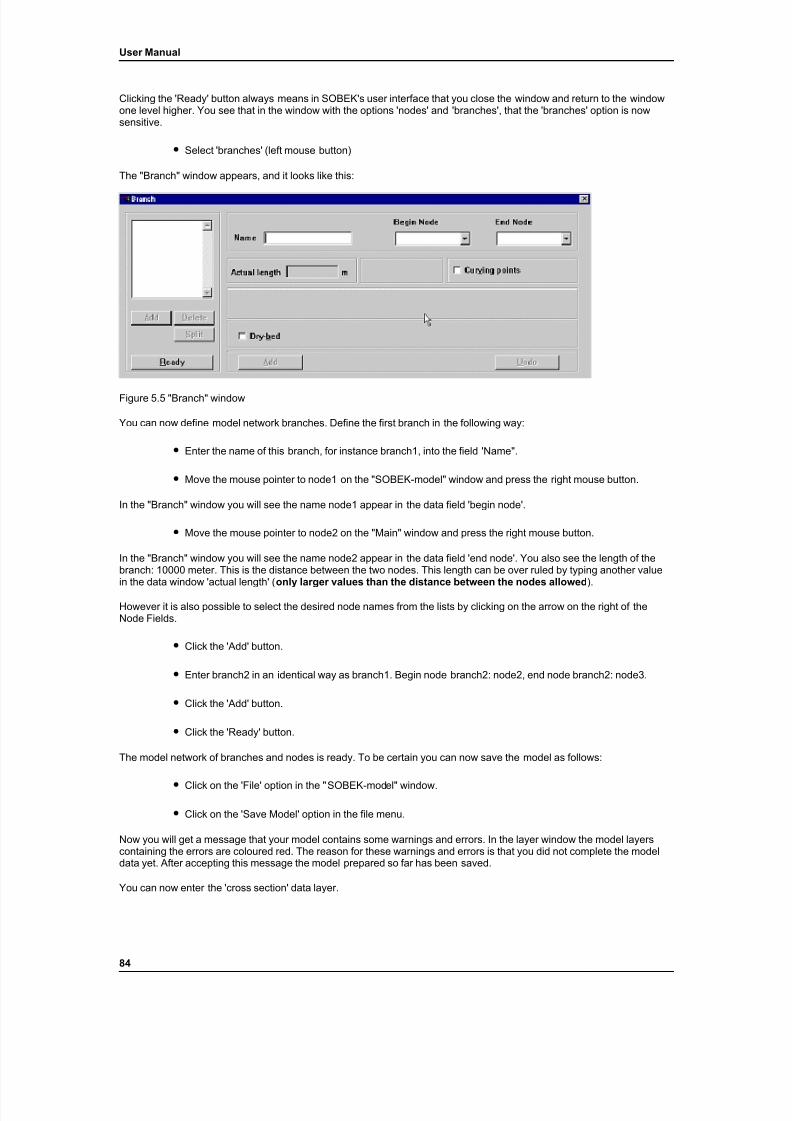
7/21/2019 SOBEK - UserManual
http://slidepdf.com/reader/full/sobek-usermanual 90/179
User Manual
Clicking the 'Ready' button always means in SOBEK's user interface that you close the window and return to the windowone level higher. You see that in the window with the options 'nodes' and 'branches', that the 'branches' option is nowsensitive.
• Select 'branches' (left mouse button)
The "Branch" window appears, and it looks like this:
Figure 5.5 "Branch" window
You can now define model network branches. Define the first branch in the following way:
• Enter the name of this branch, for instance branch1, into the field 'Name".
• Move the mouse pointer to node1 on the "SOBEK-model" window and press the right mouse button.
In the "Branch" window you will see the name node1 appear in the data field 'begin node'.
• Move the mouse pointer to node2 on the "Main" window and press the right mouse button.
In the "Branch" window you will see the name node2 appear in the data field 'end node'. You also see the length of thebranch: 10000 meter. This is the distance between the two nodes. This length can be over ruled by typing another valuein the data window 'actual length' ( only larger values than the distance between the nodes allowed ).
However it is also possible to select the desired node names from the lists by clicking on the arrow on the right of theNode Fields.
• Click the 'Add' button.
• Enter branch2 in an identical way as branch1. Begin node branch2: node2, end node branch2: node3.
• Click the 'Add' button.
• Click the 'Ready' button.
The model network of branches and nodes is ready. To be certain you can now save the model as follows:
• Click on the 'File' option in the "SOBEK-model" window.
• Click on the 'Save Model' option in the file menu.
Now you will get a message that your model contains some warnings and errors. In the layer window the model layerscontaining the errors are coloured red. The reason for these warnings and errors is that you did not complete the modeldata yet. After accepting this message the model prepared so far has been saved.
You can now enter the 'cross section' data layer.
84

7/21/2019 SOBEK - UserManual
http://slidepdf.com/reader/full/sobek-usermanual 91/179
User Manual
Cross sections
• Select the data layer 'cross sections' by clicking the corresponding radio button in the 'Select Layer'window (edit button).
A window pops up with two options: 'Descriptions' and 'Cross Sections'. The cross section definition in SOBEK is dividedin two parts: under 'descriptions' you define the shape of each cross section and make a list of cross section descriptions
and under 'cross sections' you define cross sections in your model by giving them a co-ordinate in the model network andselecting one of the descriptions made under the 'descriptions' option.
You will see that the option 'cross sections' is insensitive, because no descriptions have yet been made.
Note that the "topography" window disappears. Remember: you can only edit one data layer at the time. This restrictionhas been implemented for your convenience: if it would be released there could be a great risk that the user soon losestrack of what he is doing.
• Select 'descriptions' (left mouse button)
The data window "cross section description" appears. Note the similarity to the "nodes" and "branches" windows. Thisappearance of data windows will come back several times.
Now, you are going to define the cross section as given in Figure 5.2.
• Click the radio button 'Trapezoid'
You should type the appropriate data into the various data fields. You can jump from one data field to another by pressingthe « TAB » key on the keyboard, or by moving the mouse pointer to the next field and pressing the left mouse button.
• Enter the 'Bed level': –3 m and press « TAB »
• Enter the 'Bottom width': 45 m and press « TAB »
• Enter the 'Bank slope': 3 (this gives a bank slope 1:3 on both sides of the channel) and press « TAB »
• Enter the 'Maximum flow width': 75 m and press « TAB »
The maximum flow width indicates the extension of the bank slopes. If during a simulation the water level would rise
above the level corresponding with a width of 75 metres, SOBEK assumes vertical bounds from that level onward.
• Enter the 'Width of the main channel': 45 m and press « TAB »
• Enter the 'Width of floodplain 1': 30 m and press « TAB »
Note that in this case floodplain 1 is not actually a floodplain, it is only a part of the cross section with a differentroughness.
The width of floodplain 2 is computed by the program. In this case it will be zero.
At this moment the window should look like this:
85
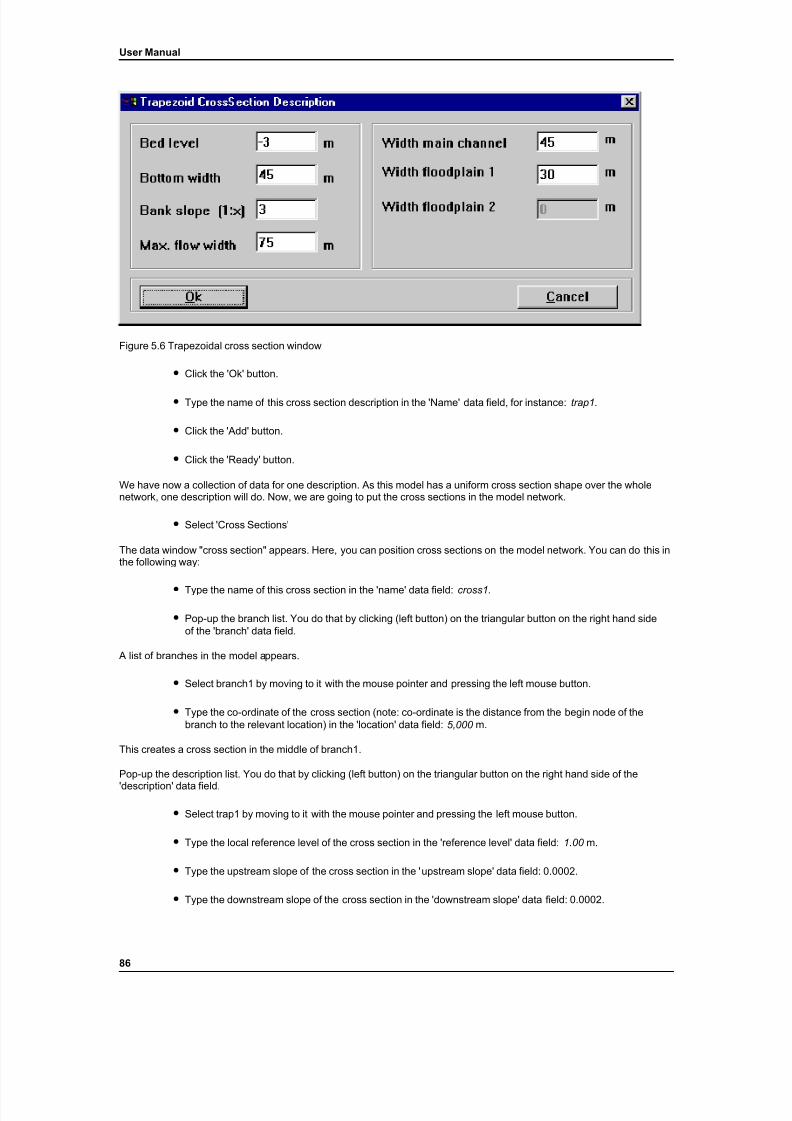
7/21/2019 SOBEK - UserManual
http://slidepdf.com/reader/full/sobek-usermanual 92/179
User Manual
Figure 5.6 Trapezoidal cross section window
• Click the 'Ok' button.
• Type the name of this cross section description in the 'Name' data field, for instance: trap1 .
• Click the 'Add' button.
• Click the 'Ready' button.
We have now a collection of data for one description. As this model has a uniform cross section shape over the wholenetwork, one description will do. Now, we are going to put the cross sections in the model network.
• Select 'Cross Sections'
The data window "cross section" appears. Here, you can position cross sections on the model network. You can do this inthe following way:
• Type the name of this cross section in the 'name' data field: cross1 .
• Pop-up the branch list. You do that by clicking (left button) on the triangular button on the right hand sideof the 'branch' data field.
A list of branches in the model appears.
• Select branch1 by moving to it with the mouse pointer and pressing the left mouse button.
• Type the co-ordinate of the cross section (note: co-ordinate is the distance from the begin node of thebranch to the relevant location) in the 'location' data field: 5,000 m.
This creates a cross section in the middle of branch1.
Pop-up the description list. You do that by clicking (left button) on the triangular button on the right hand side of the
'description' data field.
• Select trap1 by moving to it with the mouse pointer and pressing the left mouse button.
• Type the local reference level of the cross section in the 'reference level' data field: 1.00 m.
• Type the upstream slope of the cross section in the 'upstream slope' data field: 0.0002.
• Type the downstream slope of the cross section in the 'downstream slope' data field: 0.0002.
86
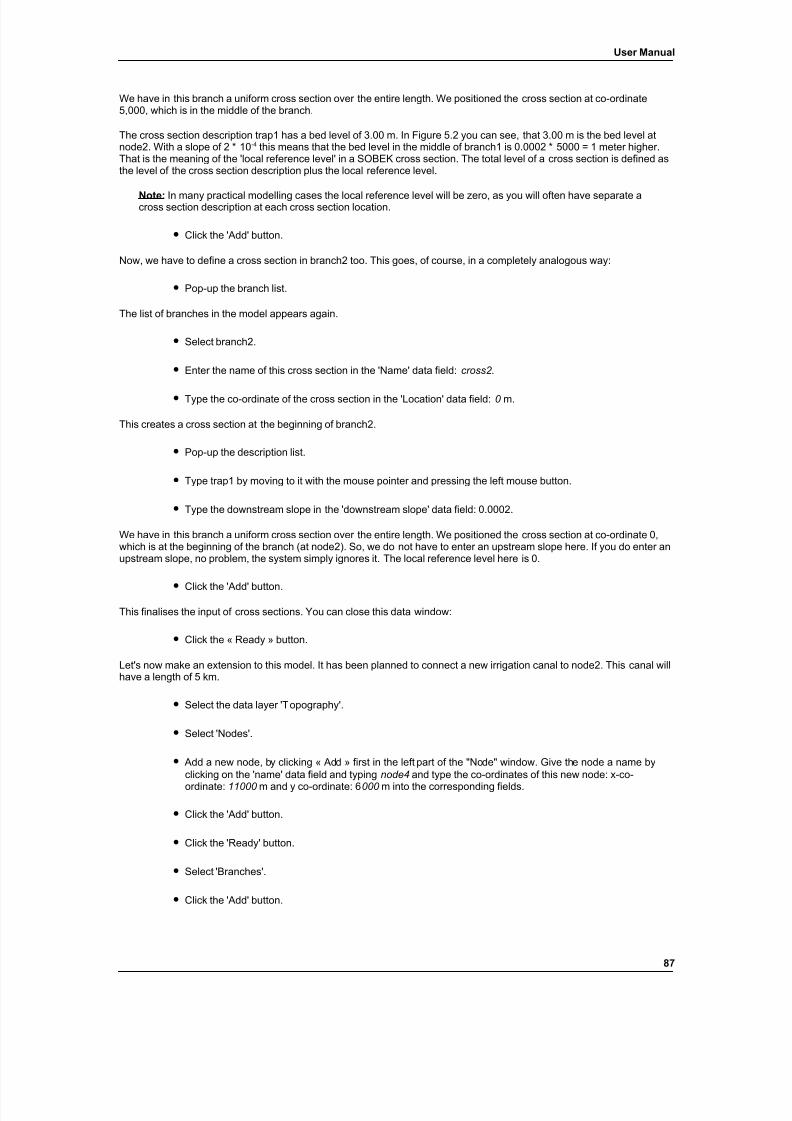
7/21/2019 SOBEK - UserManual
http://slidepdf.com/reader/full/sobek-usermanual 93/179
User Manual
We have in this branch a uniform cross section over the entire length. We positioned the cross section at co-ordinate5,000, which is in the middle of the branch.
The cross section description trap1 has a bed level of 3.00 m. In Figure 5.2 you can see, that 3.00 m is the bed level atnode2. With a slope of 2 * 10 -4 this means that the bed level in the middle of branch1 is 0.0002 * 5000 = 1 meter higher.That is the meaning of the 'local reference level' in a SOBEK cross section. The total level of a cross section is defined asthe level of the cross section description plus the local reference level.
Note: In many practical modelling cases the local reference level will be zero, as you will often have separate across section description at each cross section location.
• Click the 'Add' button.
Now, we have to define a cross section in branch2 too. This goes, of course, in a completely analogous way:
• Pop-up the branch list.
The list of branches in the model appears again.
• Select branch2.
• Enter the name of this cross section in the 'Name' data field: cross2 .
• Type the co-ordinate of the cross section in the 'Location' data field: 0 m.
This creates a cross section at the beginning of branch2.
• Pop-up the description list.
• Type trap1 by moving to it with the mouse pointer and pressing the left mouse button.
• Type the downstream slope in the 'downstream slope' data field: 0.0002.
We have in this branch a uniform cross section over the entire length. We positioned the cross section at co-ordinate 0,which is at the beginning of the branch (at node2). So, we do not have to enter an upstream slope here. If you do enter anupstream slope, no problem, the system simply ignores it. The local reference level here is 0.
• Click the 'Add' button.
This finalises the input of cross sections. You can close this data window:
• Click the « Ready » button.
Let's now make an extension to this model. It has been planned to connect a new irrigation canal to node2. This canal willhave a length of 5 km.
• Select the data layer 'Topography'.
• Select 'Nodes'.
• Add a new node, by clicking « Add » first in the left part of the "Node" window. Give the node a name byclicking on the 'name' data field and typing node4 and type the co-ordinates of this new node: x-co-ordinate: 11000 m and y co-ordinate: 6 000 m into the corresponding fields.
• Click the 'Add' button.
• Click the 'Ready' button.
• Select 'Branches'.
• Click the 'Add' button.
87
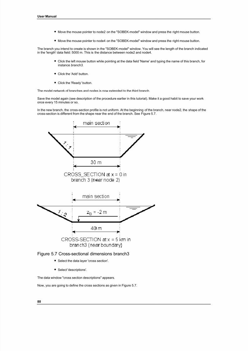
7/21/2019 SOBEK - UserManual
http://slidepdf.com/reader/full/sobek-usermanual 94/179
User Manual
• Move the mouse pointer to node2 on the "SOBEK-model" window and press the right mouse button.
• Move the mouse pointer to node4 on the "SOBEK-model" window and press the right mouse button.
The branch you intend to create is shown in the "SOBEK-model" window. You will see the length of the branch indicatedin the 'length' data field: 5000 m. This is the distance between node2 and node4.
• Click the left mouse button while pointing at the data field 'Name' and typing the name of this branch, for instance branch3 .
• Click the 'Add' button.
• Click the 'Ready' button.
The model network of branches and nodes is now extended to the third branch.
Save the model again (see description of the procedure earlier in this tutorial). Make it a good habit to save your workonce every 15 minutes or so.
In the new branch, the cross-section profile is not uniform. At the beginning of the branch, near node2, the shape of thecross-section is different from the shape near the end of the branch. See Figure 5.7.
Figure 5.7 Cross-sectional dimensions branch3• Select the data layer 'cross section'.
• Select 'descriptions'.
The data window "cross section descriptions" appears.
Now, you are going to define the cross sections as given in Figure 5.7.
88
7/21/2019 SOBEK - UserManual
http://slidepdf.com/reader/full/sobek-usermanual 95/179
User Manual
• Click the « Add » button on the left side of the "Cross section descriptions" window.
• Type the name of this description in the 'name' data field, for instance: trap2 .
• Click the radio button 'Trapezoid'
• Type the 'Bed level': –2 m and press « TAB »
• Type the 'Bottom width': 30 m and press « TAB »
• Type the 'Bank slope': 1 (this gives a slope 1:1) and press « TAB »
• Type the 'Maximum flow width': 40 m and press « TAB »
• Type the 'Width of the main stream': 30 m and press « TAB »
• Type the 'Width of floodplain 1': 10 m and press « TAB »
The width of floodplain 2 is computed by the program. In this case it will be zero.
• Click the 'Ok' button.
• Click the 'Add' button.
• Type the name of this description in the 'Name' data field, for instance: trap3 .
• Click the radio button 'Trapezoid'
• Type the 'Bed level': -2 m and press « TAB »
• Type the 'Bottom width': 40 m and press « TAB »
• Type the 'Bank slope': 2 (this gives a slope 1:2) and press « TAB »
• Type the 'Maximum flow width': 60 m and press « TAB »
• Type the 'Width of the main stream': 40 m and press « TAB »
• Type the 'Width of floodplain 1': 20 m and press « TAB »
• Click the 'Ok' button.
• Click the 'Add' button.
• Click the 'Ready' button.
We now have extended the collection of cross section descriptions to a total number of three.
• Select 'Cross sections'.
• Click the « Add » button on the left side of the "Cross sections" window.
• Type the name of this cross section in the 'name' data field: cross3.
• Pop-up the branch list.
A list of branches in the model appears. This list now contains three branches.
89
7/21/2019 SOBEK - UserManual
http://slidepdf.com/reader/full/sobek-usermanual 96/179
User Manual
• Select branch3 by moving to it with the mouse pointer and pressing the left mouse button.
• Type the co-ordinate of the cross section in the 'Location' data field: 0 m.
This creates a cross section at the beginning of branch3.
• Pop-up the description list.
• Select trap2.
We do not have to enter an upstream or downstream slope here: at the end of the branch we will define another crosssection and the system will interpolate between these two to generate cross-sections in the branch.
• Click the 'Add' button.
• Type the name of this cross section in the 'Name' data field: cross4 .
• Pop up the branch list.
• Select branch3.
• Type the co-ordinate of the cross section in the 'Location' data field: 5,000 m.
This creates a cross section at the end of branch3.
• Pop-up the description list.
• Select trap3.
• Click the 'Add' button.
• Click the « Ready » button.
The next step is entering the boundary conditions for the model. This is not compulsory: you can also first enter bedroughness ('Friction' layer), hydraulics structures or any other data you prefer. The sequence of entry is up to you!
Next, we are going to define a hydraulic structure in branch3, the new canal. The discharge in this canal is controlled by agate.
Structures
• Select 'structures' from the "Select layer" window (radio button).
A window appears with five options: 'descriptions', 'controllers', 'triggers', 'structures' and 'compound'. The procedure isfully analogous to the cross sections. First you define one or more hydraulic structure descriptions and then you can usethese structures everywhere in your model.
• Select 'Descriptions'.
The "Structure description" window pops up.
• Type the name, for instance gate1 in the 'name' data field.
• Select 'General' by clicking the corresponding radio button.
The "General structure description" window appears with some data fields to define the dimensions of the structure. SeeFigure 5.12.
90

7/21/2019 SOBEK - UserManual
http://slidepdf.com/reader/full/sobek-usermanual 97/179
User Manual
Figure 5.12 Gate in branch3The crest level is –1.00 m and the crest width is 15 m. The gate opening is 1.5 m.
• Type the crest width in the 'W1, Wsdl, Ws, Wsdr and W2' data fields: 15m.
• Give the gate opening: 1.50 m.
• Type the crest level in the 'zb1, zbsl, zbs, zbsr and zb2' data fields: –1.00 m.
• Give all the discharge coefficients for Flow and Reverse Flow a value of 1.0.
Note: T he general structure offers more complicated geometry. Here we apply a structure with very simplegeometry, which forces us to enter the same width and level a few times (see TRM-General Structure)
• Click the « Ok » button.
• Click the « Add » button.
• Click the « Ready » button.
Now enter the 'structures' option and put the structure at its proper location.
• Select 'structures'.
The data window "Structures" appears. Here, you can position hydraulic structures on the model network. You can do thisas follows (note: this is fully analogous to the cross sections procedure!):
• Enter the name of this structure in the 'Name' data field: gate branch3 .
91
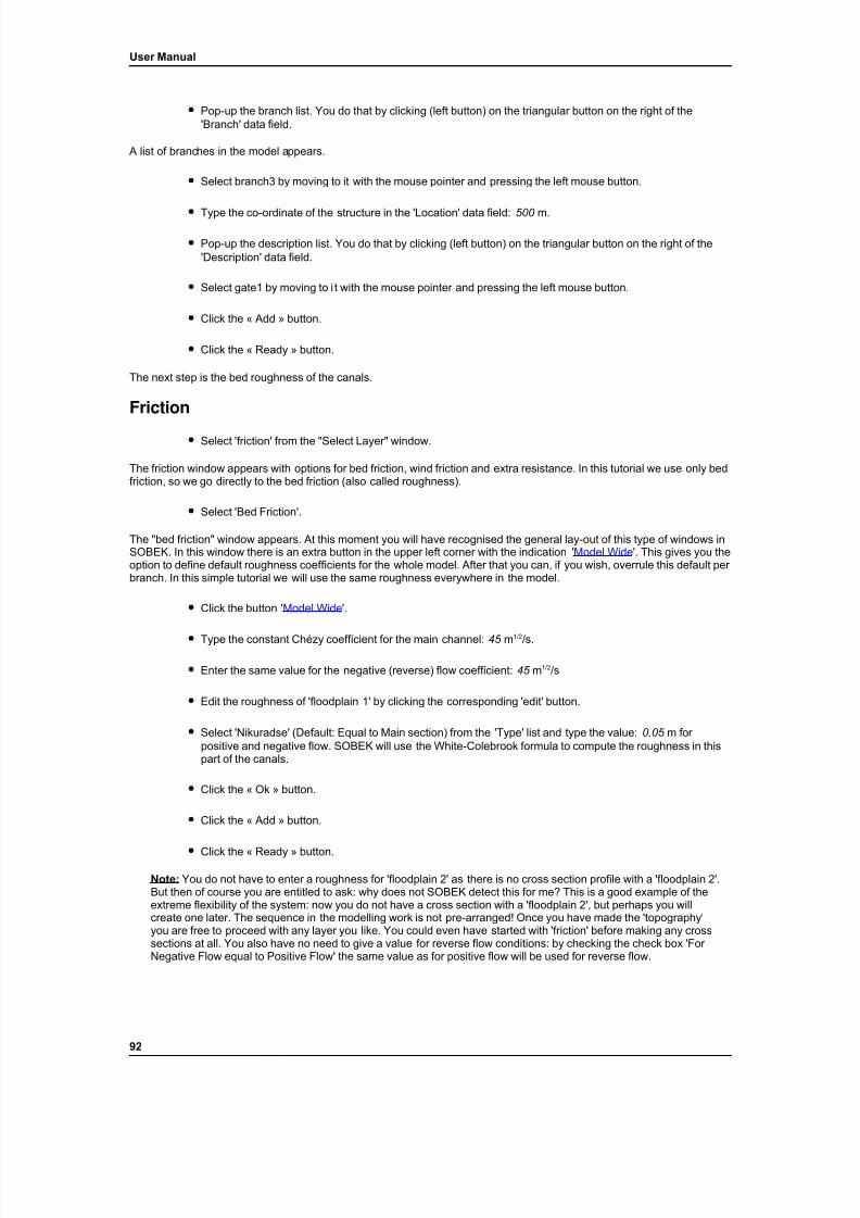
7/21/2019 SOBEK - UserManual
http://slidepdf.com/reader/full/sobek-usermanual 98/179
User Manual
• Pop-up the branch list. You do that by clicking (left button) on the triangular button on the right of the'Branch' data field.
A list of branches in the model appears.
• Select branch3 by moving to it with the mouse pointer and pressing the left mouse button.
• Type the co-ordinate of the structure in the 'Location' data field: 500 m.
• Pop-up the description list. You do that by clicking (left button) on the triangular button on the right of the'Description' data field.
• Select gate1 by moving to i t with the mouse pointer and pressing the left mouse button.
• Click the « Add » button.
• Click the « Ready » button.
The next step is the bed roughness of the canals.
Friction
• Select 'friction' from the "Select Layer" window.
The friction window appears with options for bed friction, wind friction and extra resistance. In this tutorial we use only bedfriction, so we go directly to the bed friction (also called roughness).
• Select 'Bed Friction'.
The "bed friction" window appears. At this moment you will have recognised the general lay-out of this type of windows inSOBEK. In this window there is an extra button in the upper left corner with the indication 'Model Wide '. This gives you theoption to define default roughness coefficients for the whole model. After that you can, if you wish, overrule this default per branch. In this simple tutorial we will use the same roughness everywhere in the model.
• Click the button 'Model Wide '.
• Type the constant Chézy coefficient for the main channel: 45 m1/2
/s.
• Enter the same value for the negative (reverse) flow coefficient: 45 m 1/2 /s
• Edit the roughness of 'floodplain 1' by clicking the corresponding 'edit' button.
• Select 'Nikuradse' (Default: Equal to Main section) from the 'Type' list and type the value: 0.05 m for positive and negative flow. SOBEK will use the White-Colebrook formula to compute the roughness in thispart of the canals.
• Click the « Ok » button.
• Click the « Add » button.
• Click the « Ready » button.
Note: You do not have to enter a roughness for 'floodplain 2' as there is no cross section profile with a 'floodplain 2'.But then of course you are entitled to ask: why does not SOBEK detect this for me? This is a good example of theextreme flexibility of the system: now you do not have a cross section with a 'floodplain 2', but perhaps you willcreate one later. The sequence in the modelling work is not pre-arranged! Once you have made the 'topography'you are free to proceed with any layer you like. You could even have started with 'friction' before making any crosssections at all. You also have no need to give a value for reverse flow conditions: by checking the check box 'For Negative Flow equal to Positive Flow' the same value as for positive flow will be used for reverse flow.
92
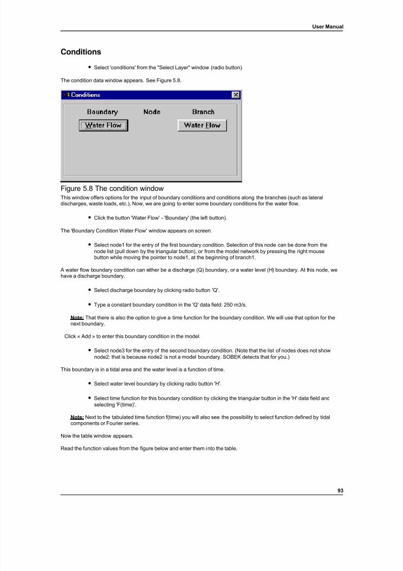
7/21/2019 SOBEK - UserManual
http://slidepdf.com/reader/full/sobek-usermanual 99/179
User Manual
Conditions
• Select 'conditions' from the "Select Layer" window (radio button).
The condition data window appears. See Figure 5.8.
Figure 5.8 The condition window
This window offers options for the input of boundary conditions and conditions along the branches (such as lateraldischarges, waste loads, etc.). Now, we are going to enter some boundary conditions for the water flow.
• Click the button 'Water Flow' - 'Boundary' (the left button).
The 'Boundary Condition Water Flow' window appears on screen.
• Select node1 for the entry of the first boundary condition. Selection of this node can be done from thenode list (pull down by the triangular button), or from the model network by pressing the right mousebutton while moving the pointer to node1, at the beginning of branch1.
A water flow boundary condition can either be a discharge (Q) boundary, or a water level (H) boundary. At this node, wehave a discharge boundary.
• Select discharge boundary by clicking radio button 'Q'.
• Type a constant boundary condition in the 'Q' data field: 250 m3/s.
Note: That there is also the option to give a time function for the boundary condition. We will use that option for thenext boundary.
Click « Add » to enter this boundary condition in the model.
• Select node3 for the entry of the second boundary condition. (Note that the list of nodes does not shownode2: that is because node2 is not a model boundary. SOBEK detects that for you.)
This boundary is in a tidal area and the water level is a function of time.
• Select water level boundary by clicking radio button 'H'.
• Select time function for this boundary condition by clicking the triangular button in the 'H' data field andselecting 'F(time)'.
Note: Next to the tabulated time function f(time) you will also see the possibility to select function defined by tidalcomponents or Fourier series.
Now the table window appears.
Read the function values from the figure below and enter them into the table.
93
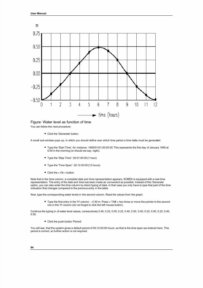
7/21/2019 SOBEK - UserManual
http://slidepdf.com/reader/full/sobek-usermanual 100/179
User Manual
Figure: Water level as function of timeYou can follow the next procedure:
• Click the 'Generate' button.
A small sub-window pops up, in which you should define over which time period a time table must be generated.
• Type the 'Start Time', for instance: 1995/01/01;00:00:00 . This represents the first day of January 1995 at
0:00 in the morning (or should we say: night).
• Type the 'Step Time': 00;01:00:00 (1 hour)
• Type the 'Time Span': 00;12:00:00 (12 hours)
• Click the « Ok » button.
Note that in the time column, a complete date and time representation appears. SOBEK is equipped with a real-timerepresentation. The entry of the date and time has been made as convenient as possible. Instead of this 'Generate'option, you can also enter the time column by direct typing of data. In that case you only have to type that part of the timeindication that changes compared to the previous entry in the table.
Now, type the corresponding water levels in the second column. Read the values from the graph.
• Type the first entry in the 'H' column: –0.50 m. Press « TAB » two times or move the pointer to the secondrow in the 'H' column (do not forget to click the left mouse button).
Continue the typing in of water level values, consecutively 0.40, 0.22, 0.00, 0.22, 0.40, 0.50, 0.40, 0.22, 0.00, 0.22, 0.40,0.50.
• Click the push-button 'Period'.
You will see, that the system gives a default period of 00;12:00:00 hours, as that is the time span we entered here. Thisperiod is correct, so further action i s not required.
94
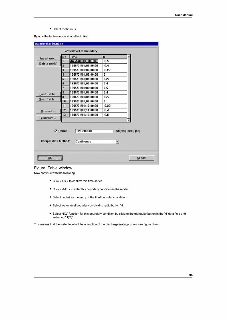
7/21/2019 SOBEK - UserManual
http://slidepdf.com/reader/full/sobek-usermanual 101/179
User Manual
• Select continuous
By now the table window should look like:
Figure: Table windowNow continue with the following:
• Click « Ok » to confirm this time series.
• Click « Add » to enter this boundary condition in the model.
• Select node4 for the entry of the third boundary condition.
• Select water level boundary by clicking radio button 'H'.
• Select H(Q) function for this boundary condition by clicking the triangular button in the 'H' data field andselecting 'H(Q)'.
This means that the water level will be a function of the discharge (rating curve), see figure blow.
95
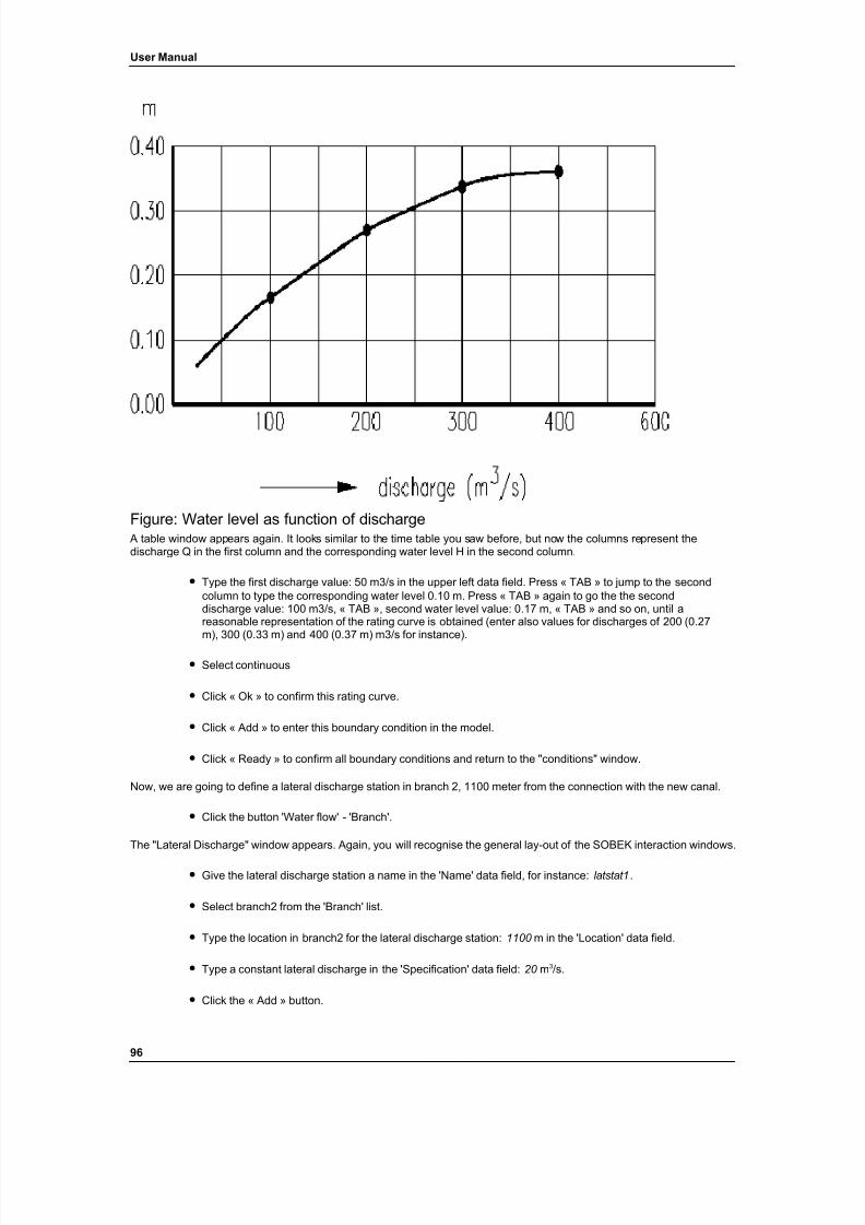
7/21/2019 SOBEK - UserManual
http://slidepdf.com/reader/full/sobek-usermanual 102/179
User Manual
Figure: Water level as function of discharge A table window appears again. It looks similar to the time table you saw before, but now the columns represent thedischarge Q in the first column and the corresponding water level H in the second column.
• Type the first discharge value: 50 m3/s in the upper left data field. Press « TAB » to jump to the secondcolumn to type the corresponding water level 0.10 m. Press « TAB » again to go the the seconddischarge value: 100 m3/s, « TAB », second water level value: 0.17 m, « TAB » and so on, until areasonable representation of the rating curve is obtained (enter also values for discharges of 200 (0.27m), 300 (0.33 m) and 400 (0.37 m) m3/s for instance).
• Select continuous
• Click « Ok » to confirm this rating curve.
• Click « Add » to enter this boundary condition in the model.
• Click « Ready » to confirm all boundary conditions and return to the "conditions" window.
Now, we are going to define a lateral discharge station in branch 2, 1100 meter from the connection with the new canal.
• Click the button 'Water flow' - 'Branch'.
The "Lateral Discharge" window appears. Again, you will recognise the general lay-out of the SOBEK interaction windows.
• Give the lateral discharge station a name in the 'Name' data field, for instance: latstat1 .
• Select branch2 from the 'Branch' list.
• Type the location in branch2 for the lateral discharge station: 1100 m in the 'Location' data field.
• Type a constant lateral discharge in the 'Specification' data field: 20 m 3/s.
• Click the « Add » button.
96
7/21/2019 SOBEK - UserManual
http://slidepdf.com/reader/full/sobek-usermanual 103/179
User Manual
• Click the « Ready » button.
There is now a constant discharge into the model of a magnitude of 20 m 3/s.
Initial conditions
• Select 'initial conditions' from the "Select layer" window (radio button).
The "Initial Condition" window appears with options to use the 'User Conditions' and 'Auto-start', for the tutorial we choose'Auto-start'.
Grid definition
We have now entered all physical data for a computation: cross sections, boundary conditions, roughness, a hydraulicstructure and the lateral discharge station. What more do we need for a water flow computation? We still need acomputational grid. Make such grid with space increments of 500 m in each branch.
• Select 'Grid Definition' from the "Select Layer" window.
• Select 'Water Flow Grid' from the "Grid Main" window.
The "Grid Data" window appears, in which you can enter a computational grid for all branches.
• Select branch1 from the 'Branch' list (you know the procedure).
• Enter the equidistant grid step in the 'Distance' data field: 500 m.
• Click the button « Generate ».
This generates an equidistant grid with increments of 500 meters in branch 1. No further action is required here, but byclicking « Edit » you can have a look at the grid steps in a table where they can be edited if required.
• Click the « Add » button to add the grid of branch1 to the grid definition.
• Now repeat the procedure for branch2 and branch3:
• Select branch2 from the 'Branch' list.
• Enter the equidistant grid step in the 'Distance' data field: 500 m. (The value is already in the data field, asit is maintained from the previous branch).
• Click the button « Generate ».
• Click the « Add » button.
• Select branch3 from the 'Branch' list.
• Type the equidistant grid step in the 'Distance' data field: 500 m. (The value is already in the data field, asit is maintained from the previous branch).
• Click the button « Generate ».
• Click the « Add » button.
• Click the « Ready » button.
97
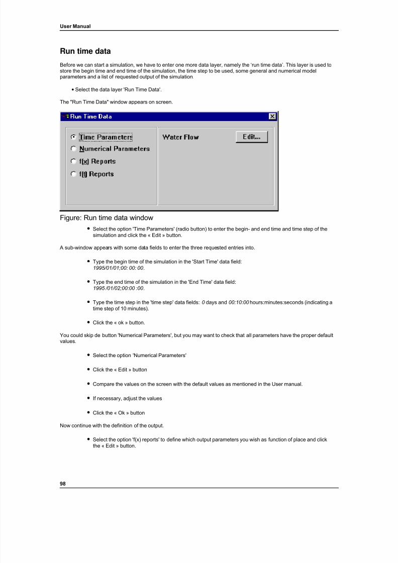
7/21/2019 SOBEK - UserManual
http://slidepdf.com/reader/full/sobek-usermanual 104/179
User Manual
Run time data
Before we can start a simulation, we have to enter one more data layer, namely the ‘run time data’. This layer is used tostore the begin time and end time of the simulation, the time step to be used, some general and numerical modelparameters and a list of requested output of the simulation.
• Select the data layer 'Run Time Data'.
The "Run Time Data" window appears on screen.
Figure: Run time data window• Select the option 'Time Parameters' (radio button) to enter the begin- and end time and time step of the
simulation and click the « Edit » button.
A sub-window appears with some data fields to enter the three requested entries into.
• Type the begin time of the simulation in the 'Start Time' data field:1995/01/01;00: 00: 00 .
• Type the end time of the simulation in the 'End Time' data field:1995 /01/02;00:00 :00 .
• Type the time step in the 'time step' data fields: 0 days and 00:10:00 hours:minutes:seconds (indicating atime step of 10 minutes).
• Click the « ok » button.
You could skip de button 'Numerical Parameters', but you may want to check that all parameters have the proper defaultvalues.
• Select the option 'Numerical Parameters'
• Click the « Edit » button
• Compare the values on the screen with the default values as mentioned in the User manual.
• If necessary, adjust the values
• Click the « Ok » button
Now continue with the definition of the output.
• Select the option 'f(x) reports' to define which output parameters you wish as function of place and clickthe « Edit » button.
98
7/21/2019 SOBEK - UserManual
http://slidepdf.com/reader/full/sobek-usermanual 105/179
User Manual
A window appears with several push buttons to activate and de-activate various output parameters. Note that, in additionto the parameters listed here, the post-processing unit will also be able to present derived information (such as the flowvelocity: discharge divided by flow area).
Next to the push buttons you will see also 'Start Time' and 'Time Step' data fields.
• Select (at least) the following quantities for output: water level and discharge by checking the concerningcheck boxes.
• If not filled in yet, enter the begin time for writing results in the 'Start Time' data field:1995/01/01;00 :00:00 (which is the beginning of the simulation).
• If not filled in yet, enter the end time for writing results in the 'End Time' data field: 1995/01/02;00:00(which is the end time of the simulation).
• Enter the time interval for writing f(x) results: 6 (this will give output every six time steps, whichcorresponds with output every hour, as the time step is 10 minutes).
• Click the « Ok » button.
Now, we are going to select the output we wish as function of time.
• Select the option 'f(t) reports' and click the « Edit » button.
A similar window to the f(x) results window appears with several push buttons to activate and de-activate various outputparameters. Next to the push buttons you also see a 'branch/location' data field.
• Select (at least) the following quantities for output: water level and discharge by checking the concerningcheck boxes.
• Add the following branch/locations for output (click the « Edit » button 'branch/locations'):
1. branch: branch1 , location: 9000 m, click « Add » button2. branch: branch2 , location: 1000 m, click « Add » button3. branch: branch3 , location: 1000 m, click « Add » button
• Click the « Ready » button.
Note, that the current window also provides options for selecting time series of parameters at structures and lateraldischarge stations. We will not use them now.
• Click the « Ok » button.
• Select the Operations->Validate option from the SOBEK Model Window to validate the model. If everything was done properly so far you will get the message 'No consistency errors found.' If not you willhave to check the data.
• Now you can save the model and leave the SOBEK Model Window.
• Run the model by double clicking the 'Hydraulic Computation' Task.
• View at the results by double clicking the 'Hydraulic Results' Task
• Save the Case by selecting 'Case' -> 'Save'.
• Leave the Case Management Tool by selecting 'Case' -> 'Exit'
• Leave SOBEK by clicking 'Exit SOBEK'.
99
7/21/2019 SOBEK - UserManual
http://slidepdf.com/reader/full/sobek-usermanual 106/179
User Manual
Appendix A (Installation & Authorization)
Installation on PC
SOBEK can be installed on computers running under the Windows-2000, Windows-XP or Windows Vista operatingsystems. The SOBEK software is available on a CD-ROM. Insert the CD-ROM and start the program SETUP.EXEavailable on this CD-ROM. Follow the instructions which will be displayed on screen.
Note: During installation under Windows 2000, XP or Vista you have to be logged on to Windows as Administrator or as a user with administrator rights. If not, you will not have the permission to install some drivers.
If the installation program encounters serious problems the installation will be terminated and a message will be issuedstating that installation is not completed. It often helps to terminate all running applications under Windows before startingthe installation program.
After installation, the following directory structure will be made for SOBEK.
x:\sobek\programs this directory contains all SOBEK softwarex:\sobek\model this directory contains the model datax:\sobek\temp this directory is for temporary files
After installing the license file (See Software Authorisation) you can start-up the SOBEK-RE system with the Start Menu.
Directory Structure
SOBEK stores the users's models in the directory %SOBEKHOME%/model.
The model directory consists of directories, one for every project.
An overview of the directory-tree is ( italics indicates user defined names):
%SOBEKHOME%\model\default.sbk (default project for initializing projects)
\project.ini (with initialization files)
\tutorial.sbk (the tutorial examle)
\ userproj. sbk (user defined project(s)
Startup directory related to 'Import/export files'
SOBEK provides the facility to import/export files (tables, cross-sections). These files are selected by the standard fileselector. The default directory in this file-selector will be the directory from which SOBEK was started.
Software authorization
This version of SOBEK can use a software key instead of a hardware key (dongle) to protect the software againstunauthorised use. The program SOBEK uses FLEXlm as license manager, which is a platform independent licensemanager. The use of a software key has the advantage that there will be no supply of a hardware key and there is noconflict with other programs which use a hardware key. Also network versions of SOBEK can be delivered. To useFLEXlm as license manager for the software, SOBEK Support will supply a license file.
FLEXlm on a Windows computer
To generate a license file we need the ethernet address (MAC-address) of the ethernet-card on the computer on whichSOBEK shall be run. The ethernet-address can be found with the program lmtools.exe which is on the %SOBEK%\Programs\License directory or through the Start ->Sobek-RE menu if Sobek-RE is already installed. Select the TAB"System Settings" . In the given list, the ethernet address is given.
100

7/21/2019 SOBEK - UserManual
http://slidepdf.com/reader/full/sobek-usermanual 107/179
User Manual
The license-file will be sent to you after it is generated and will be read by the license manager.
The default directory for license files is C:\Program Files\DS_Flex
FLEXlm daemon on a Windows server
To generate a license file we need the ethernet address (MAC-address) of the ethernet-card on the computer on whichthe Flexlm license manager is installed. The ethernet-address can be found with the program lmtools.exe which is on theC:\Program Files\DS_Flex directory or through the Start ->Sobek-RE menu if Sobek-RE is already installed. Select theTAB "System Settings" . In the given list, the ethernet address is given.
The license-file will be sent to you after it is generated and will be read by SOBEK. The place of the license file must beset by the environment variable LM_LICENSE_FILE.
The license manager and vendor daemon are placed on the directory %SOBEK%/license. Before you can use SOBEKyou have to start the license manager with the command:
%SOBEK%/license/lmgrd.exe -app.
Note: Every time the machine goes down the daemon should be restarted before it is possible to use SOBEK. Sowe advise you to install the flexlm license manager as a service (see next section).
Example:
SET SOBEK=d:\sbkSET LM_LICENSE_FILE=%SOBEK%\license\license.dat%SOBEK%/license/lmgrd.exe -app
FLEXlm License Manager as a service
To generate a license file we need the ethernet address (MAC-address) of the ethernet-card on the computer on whichthe Flexlm license manager is installed. The ethernet-address can be found with the program lmtools.exe which is on theC:|Program Files\DS_Flexe directory or through the Start ->Sobek-RE menu if Sobek-RE is already installed. Select theTAB "System Settings" . In the given list, the ethernet address is given.
The license-file will be sent to you after it is generated and will be read by SOBEK. The place of the license file must beset by the environment variable LM_LICENSE_FILE.
LMGRD .EXE can be started as an application from the Windows Server console as described in the previous section. Alternatively, LMGRD .EXE can be installed as a service on a Windows Server system so that it can be managed fromthe control panel. When using LMGRD .EXE as a service under Windows, it is sufficient to place only the licensesoftware on the Windows-Server machine.
The Sobek Helpdesk can supply you with the most recent version of the Flexlm license manager software. Install thissoftware on your Windows Server using the setup program. After installation a DS_Flex directory (defaultC:\Program Files\DS_Flex) is created . Copy the vendor deamon (dwldelft.exe) and the provided license file tothis directory.
Start the Flexlm License Manager Control, the following window will appear:
101
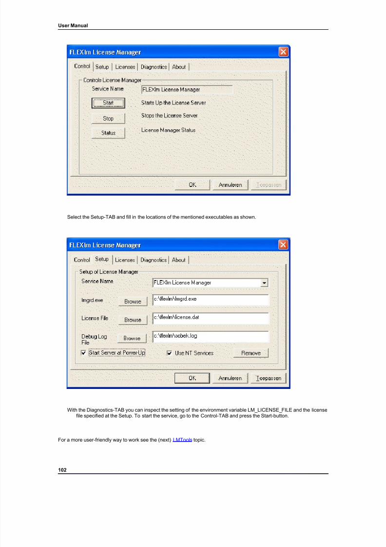
7/21/2019 SOBEK - UserManual
http://slidepdf.com/reader/full/sobek-usermanual 108/179
User Manual
Select the Setup-TAB and fill in the locations of the mentioned executables as shown.
With the Diagnostics-TAB you can inspect the setting of the environment variable LM_LICENSE_FILE and the licensefile specified at the Setup. To start the service, go to the Control-TAB and press the Start-button.
For a more user-friendly way to work see the (next) LMTools topic.
102
7/21/2019 SOBEK - UserManual
http://slidepdf.com/reader/full/sobek-usermanual 109/179
User Manual
LMTools Utility
A more user-friendly alternative to work with the FLEXlm License Manager is to use the LMTools Utility which is found inStart -> Programs ->Delft Hydraulics -> DHS License Manager (#installation type#) -> LMTools.
With this Utility you can control the license manager and also retrieve all kinds of status information like e.g. the Host-Id's.
Appendix B (Messages)SOBEK Messages
The SOBEK system may produce messages (errors and warning) on several windows. Three different message windowsare distinguished:
1. The SOBEK message window, in which regular messages appear while working with the user interface of SOBEK .
2. The SOBEK special messages window, in which messages appear after you use the 'validate model' optionor while you are working with the substances and processes definition (water quality).
3. The message window for errors and warning generated by the computational core of SOBEK . This windowis present in the 'simulation control' window.
In the following, first the user interface messages are treated. After that, the messages of the computational core arediscussed. If possible, we give a suggestion how to proceed or how to solve the problem.
Messages User Interface
Messages User Interface 0 - 999
00002 I/O error: cannot open file .....
SOBEK is not able to open the selected file. Please verify if the selected file is of the right format (e.g. ASCII or binary) and present in the proper directory.
00003 The current location is not on the branch. It is now reset to a location on the branch closest to the location youentered.
If you enter a location which is outside the length of a branch, SOBEK moves the object to the nearest by position in thebranch.
00004 You did not specify the required .... data.
The system expects you to type in data. You should specify the data or click the <<cancel>> or <<undo>> button toleave the window.
00006 I/O error: cannot create directory .....
SOBEK is not able to create the directory. It is possible that SOBEK has not been installed properly or that the directory already exists.
00007 File .... exists, overwrite this file ?
You want to save a file, but a file with the specified name already exists on the current directory. You can choose tooverwrite this old file or give the new file another na me.
00008 The .. of the Geographical Area is less then or equal to zero
The xmax value should be larger than the xmin value (the same counts for ymax and ymin).
00009 Please make sure that .. are closed.
Warning to close your post-processing or simulation window first.
00010 No cross section levels defined yet
103
7/21/2019 SOBEK - UserManual
http://slidepdf.com/reader/full/sobek-usermanual 110/179
User Manual
You press the <<view>> button, but you did not yet define the cross section description.
00011 You can visualise only .. items at the same time
The maximum number of cross sections in one graph is limited.
00012 Option Equal to main in ... not allowed
If Resistance Type is CHEZY and at least one coefficient is given as F(Q) or F(H):'EQUAL TO MAIN' not possible for Sub-Plaines.
00013 I/O error: cannot open file .... in mode .... (maybe it is write-protected?)
No further comment.
00014 I/O error: error [code] when writing file (maybe the file system is full?)
No further comment.
00016 I/O error: cannot create file ....
Maybe file already exists.
00017 I/O error: cannot save file .... as ....
Source file not found or target file already exists.
00018 I/O error: cannot create backup file .... for file ....
Source file not found or target backup file already exists.
00019 I/O error: cannot remove file ....
File does not exist or no permission to delete.
00020 When selecting F(Q) for one direction, the other must be F(Q) or Constant
When a variable for one direction is defined as F(Q), it has to be defined as F(Q) for the other direction as well or as aconstant.
00022 When selecting F(h) for one direction, the other must be F(h) or Constant
When a variable for one direction is defined as F(h), it has to be defined as F(h) for the other direction as well or as aconstant.
Messages User Interface 1000 - 1999
01000 A branch may not have the same begin and end node.
The begin node of a branch may never be the same one as the end node of that branch: the computational core of SOBEK can not deal with that. So please specify another node as begin or end node.
01002 You cannot delete node ...., it is begin/end node of a branch
SOBEK does not allow you to delete this node, because it figures as a begin or end node of at least one branch. Deleting the node would leave the branch with an incomplete definition. Delete the connected branch before deleting thenode.
01003 Branch "…." (….) is < the distance betweenits begin- and end node (here: ….)
The distance between the begin- and end node of a branch is computed based on the x- and y-position of both nodes.This is allowed, just be aware of this.
01004 You cannot move an existing branch
104
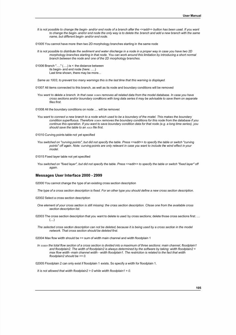
7/21/2019 SOBEK - UserManual
http://slidepdf.com/reader/full/sobek-usermanual 111/179
User Manual
It is not possible to change the begin- and/or end node of a branch after the <<add>> button has been used. If you want to change the begin- and/or end node the only way is to delete the branch and add a new branch with the samename, but different begin- and/or end node.
01005 You cannot have more then two 2D morphology branches starting in the same node
It is not possible to distribute the sediment and water discharge in a node in a proper way in case you have two 2Dmorphology branches starting in that node. You can work around this limitation by introducing a short normal
branch between the node and one of the 2D morphology branches.
01006 Branch "…." (….) is < the distance betweenits begin- and end node (here: ….)Last time shown, there may be more...
Same as 1003, to prevent too many warnings this is the last time that this warning is displayed.
01007 All items connected to this branch, as well as its node and boundary conditions will be removed
You want to delete a branch. In that case SOBEK removes all related data from the model database. In case you havecross sections and/or boundary conditions with long data series it may be advisable to save them on separatefiles first.
01008 All the boundary conditions on node .... will be removed
You want to connect a new branch to a node which used to be a boundary of the model. This makes the boundary condition superfluous. Therefore SOBEK removes the boundary conditions for this node from the database if youcontinue this operation. If you want to save boundary condition data for that node (e.g. a long time series), youshould save the table to an ASCII file first.
01010 Curving points table not yet specified
You switched on "curving points", but did not specify the table. Press <<edit>> to specify the table or switch "curving points" off again. Note: curving points are only relevant in case you want to include the wind effect in your model.
01015 Fixed layer table not yet specified
You switched on "fixed layer", but did not specify the table. Press <<edit>> to specify the table or switch "fixed layer" off again.
Messages User Interface 2000 - 299902000 You cannot change the type of an existing cross section description
The type of a cross section description is fixed. For an other type you should define a new cross section description.
02002 Select a cross section description
One element of your cross section i s still missing: the cross section description. Chose one from the available crosssection description list.
02003 The cross section description that you want to delete is used by cross sections; delete those cross sections first: ....(....)
The selected cross section description can not be deleted, because it is being used by a cross section in the model network. That cross section should be deleted first.
02004 Max flow width should be >= sum of width main channel and width floodplain 1
In SOBEK the total flow section of a cross section is divided into a maximum of three sections: main channel, floodplain1and floodplain2. The width of floodplain2 is always determined by the software by taking: width floodplain2 =max flow width -main channel width - width floodplain1. The restriction is related to the fact that widthfloodplain2 should be >= 0.
02005 Floodplain 2 can only exist if floodplain 1 exists. So specify a width for floodplain 1.
It is not allowed that width floodplain2 > 0 while width floodplain1 = 0.
105
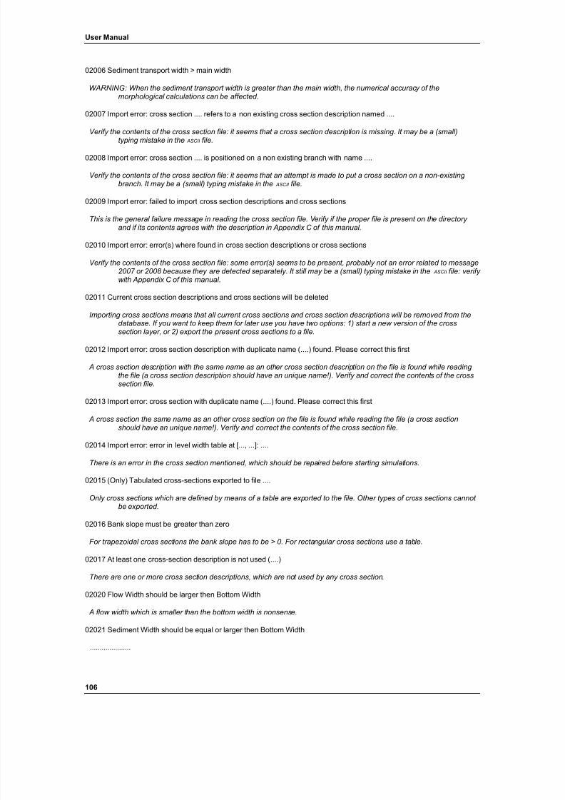
7/21/2019 SOBEK - UserManual
http://slidepdf.com/reader/full/sobek-usermanual 112/179
User Manual
02006 Sediment transport width > main width
WARNING: When the sediment transport width is greater than the main width, the numerical accuracy of themorphological calculations can be affected.
02007 Import error: cross section .... refers to a non existing cross section description named ....
Verify the contents of the cross section file: it seems that a cross section description is missing. It may be a (small)
typing mistake in the ASCII file.
02008 Import error: cross section .... is positioned on a non existing branch with name ....
Verify the contents of the cross section file: it seems that an attempt is made to put a cross section on a non-existing branch. It may be a (small) typing mistake in the ASCII file.
02009 Import error: failed to import cross section descriptions and cross sections
This is the general failure message in reading the cross section file. Verify if the proper file is present on the directory and if its contents agrees with the description in Appendix C of this manual.
02010 Import error: error(s) where found in cross section descriptions or cross sections
Verify the contents of the cross section file: some error(s) seems to be present, probably not an error related to message2007 or 2008 because they are detected separately. It still may be a (small) typing mistake in the ASCII file: verify
with Appendix C of this manual.
02011 Current cross section descriptions and cross sections will be deleted
Importing cross sections means that all current cross sections and cross section descriptions will be removed from thedatabase. If you want to keep them for later use you have two options: 1) start a new version of the crosssection layer, or 2) export the present cross sections to a file.
02012 Import error: cross section description with duplicate name (....) found. Please correct this first
A cross section description with the same name as an other cross section description on the file is found while reading the file (a cross section description should have an unique name!). Verify and correct the contents of the crosssection file.
02013 Import error: cross section with duplicate name (....) found. Please correct this first
A cross section the same name as an other cross section on the file is found while reading the file (a cross sectionshould have an unique name!). Verify and correct the contents of the cross section file.
02014 Import error: error in level width table at [..., ...]: ....
There is an error in the cross section mentioned, which should be repaired before starting simulations.
02015 (Only) Tabulated cross-sections exported to file ....
Only cross sections which are defined by means of a table are exported to the file. Other types of cross sections cannot be exported.
02016 Bank slope must be greater than zero
For trapezoidal cross sections the bank slope has to be > 0. For rectangular cross sections use a table.
02017 At least one cross-section description is not used (....)
There are one or more cross section descriptions, which are not used by any cross section.
02020 Flow Width should be larger then Bottom Width
A flow width which is smaller than the bottom width is nonsense.
02021 Sediment Width should be equal or larger then Bottom Width
.....................
106
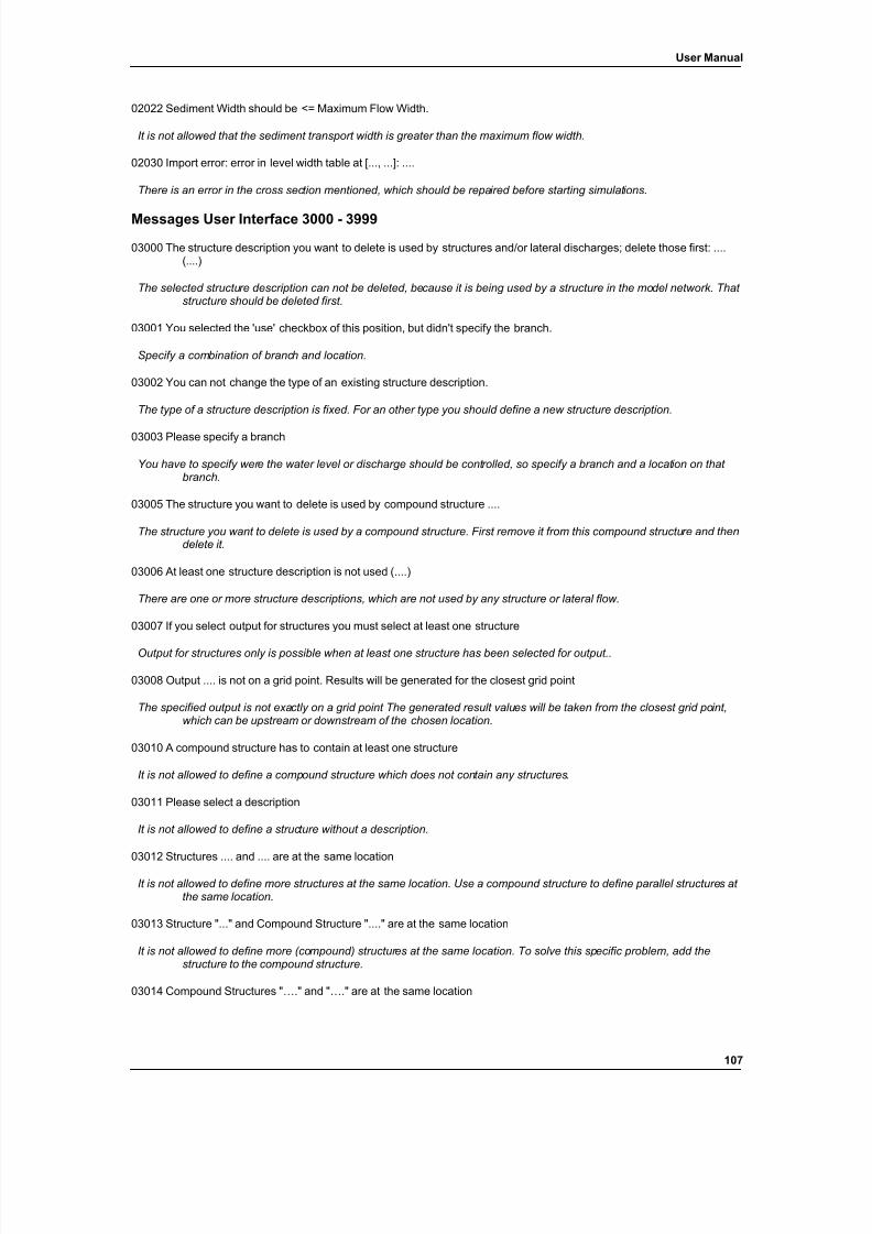
7/21/2019 SOBEK - UserManual
http://slidepdf.com/reader/full/sobek-usermanual 113/179
User Manual
02022 Sediment Width should be <= Maximum Flow Width.
It is not allowed that the sediment transport width is greater than the maximum flow width.
02030 Import error: error in level width table at [..., ...]: ....
There is an error in the cross section mentioned, which should be repaired before starting simulations.
Messages User Interface 3000 - 3999
03000 The structure description you want to delete is used by structures and/or lateral discharges; delete those first: ....(....)
The selected structure description can not be deleted, because it is being used by a structure in the model network. That structure should be deleted first.
03001 You selected the 'use' checkbox of this position, but didn't specify the branch.
Specify a combination of branch and location.
03002 You can not change the type of an existing structure description.
The type of a structure description is fixed. For an other type you should define a new structure description.
03003 Please specify a branch
You have to specify were the water level or discharge should be controlled, so specify a branch and a location on that branch.
03005 The structure you want to delete is used by compound structure ....
The structure you want to delete is used by a compound structure. First remove it from this compound structure and thendelete it.
03006 At least one structure description is not used (....)
There are one or more structure descriptions, which are not used by any structure or lateral flow.
03007 If you select output for structures you must select at least one structure
Output for structures only is possible when at least one structure has been selected for output..
03008 Output .... is not on a grid point. Results will be generated for the closest grid point
The specified output is not exactly on a grid point The generated result values will be taken from the closest grid point,which can be upstream or downstream of the chosen location.
03010 A compound structure has to contain at least one structure
It is not allowed to define a compound structure which does not contain any structures.
03011 Please select a description
It is not allowed to define a structure without a description.
03012 Structures .... and .... are at the same location
It is not allowed to define more structures at the same location. Use a compound structure to define parallel structures at the same location.
03013 Structure "..." and Compound Structure "...." are at the same location
It is not allowed to define more (compound) structures at the same location. To solve this specific problem, add thestructure to the compound structure.
03014 Compound Structures "…." and "…." are at the same location
107
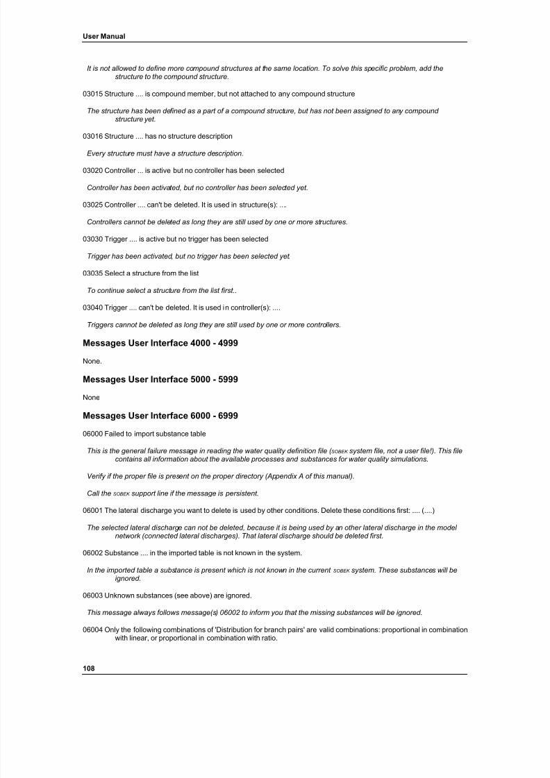
7/21/2019 SOBEK - UserManual
http://slidepdf.com/reader/full/sobek-usermanual 114/179
User Manual
It is not allowed to define more compound structures at the same location. To solve this specific problem, add thestructure to the compound structure.
03015 Structure .... is compound member, but not attached to any compound structure
The structure has been defined as a part of a compound structure, but has not been assigned to any compound structure yet.
03016 Structure .... has no structure description
Every structure must have a structure description.
03020 Controller ... is active but no controller has been selected
Controller has been activated, but no controller has been selected yet.
03025 Controller .... can't be deleted. It is used in structure(s): ....
Controllers cannot be deleted as long they are still used by one or more structures.
03030 Trigger .... is active but no trigger has been selected
Trigger has been activated, but no trigger has been selected yet.
03035 Select a structure from the list
To continue select a structure from the list first..
03040 Trigger .... can't be deleted. It is used in controller(s): ....
Triggers cannot be deleted as long they are still used by one or more controllers.
Messages User Interface 4000 - 4999
None.
Messages User Interface 5000 - 5999
None
Messages User Interface 6000 - 6999
06000 Failed to import substance table
This is the general failure message in reading the water quality definition file ( SOBEK system file, not a user file!). This filecontains all information about the available processes and substances for water quality simulations.
Verify if the proper file is present on the proper directory (Appendix A of this manual).
Call the SOBEK support line if the message is persistent.
06001 The lateral discharge you want to delete is used by other conditions. Delete these conditions first: .... (....)
The selected lateral discharge can not be deleted, because it is being used by an other lateral discharge in the model network (connected lateral discharges). That lateral discharge should be deleted first.
06002 Substance .... in the imported table is not known in the system.
In the imported table a substance is present which is not known in the current SOBEK system. These substances will beignored.
06003 Unknown substances (see above) are ignored.
This message always follows message(s) 06002 to inform you that the missing substances will be ignored.
06004 Only the following combinations of 'Distribution for branch pairs' are valid combinations: proportional in combinationwith linear, or proportional in combination with ratio.
108
7/21/2019 SOBEK - UserManual
http://slidepdf.com/reader/full/sobek-usermanual 115/179
User Manual
Distribution of the sediment transport at bifurcation can be defined in several ways in SOBEK , see the Technical ReferenceManual. When different possible bifurcating branches are possible in a node, not all possible combinations of distribution functions are possible.
06005 Failed to import water quality at boundary table
Please check the contents of the import file.
06006 Failed to import water quality at branch table
Please check the contents of the import file.
Messages User Interface 7000 - 7999
07000 You did not choose a Transport Formula for branch .... yet. Remem ber that not all grain size data D** are relevantfor each transport formu la.
When you enter the grain size curves here, and select a transport formula in a later stage, you may have typed superfluous data. For instance the Engelund and Hansen transport formula uses the D50 only and possibleinput for the other fractions is ignored. If you select the transport formula first, only the relevant grain fraction isshowed here.
07001 You did not choose a transport formula for branch ….Grain sizes according to the model wide transport formulae will be requested.
……………….
Messages User Interface 8000 - 8999
None.
Messages User Interface 9000 - 9999
None.
Messages User Interface 10000 - 10999
10000 You switched to option ...., while you defined at least one table with option ..... All the tables you defined for thisoption will be removed and will have to be re defined for the new option you chose.
This is a warning that tables defined for an old option will be removed from the model database. You can prevent that by defining a new version of this data layer and save the original option and its table in the old version of this datalayer.
Messages User Interface 11000 - 11999
11000 First select a branch to generate grid points
Grid point are defined per branch, so you should select a branch first from the list box or the model network.
11001 The distance you entered (....) exceeds the length of branch .... (....)
The location outside the length of the branch: please specify a location on the branch. You can verify the actual length of the branch in the branch window of the topography data layer.
11002 You did not enter the grid distance
A simulation can only start when a computational grid is defined for all branches first.
11003 You changed the branch. The grid points you defined earlier are of no use any more on the new branch. Delete thegrid points you defined?
All grid points have a location on a branch. As soon as you change the length of the branch, the grid of that branch may become inadequate. To make sure all branches have a proper grid, the present grid will be removed and youare requested to re-define it.
109
7/21/2019 SOBEK - UserManual
http://slidepdf.com/reader/full/sobek-usermanual 116/179
User Manual
11004 Please change 'New Segment Name' into a meaningful name
After adding a segment limit, a new segment is introduced, which gets the default name 'new segment name', which is,of course, not a very meaningful name. For that reason SOBEK asks you to give a relevant name for the new segment.
11005 You already defined grid points on this branch. Overwrite these grid points?
A simple warning that you are about to delete the old grid definition for the selected branch. You can prevent that by defining a new version of the grid layer and save the original grid in the old version of this data layer.
11006 You are about to generate several new segment limits. Do you want to REPLACE the existing limits or ADD thenew limits?
SOBEK detects an action (for instance the creation of a new branch), which will lead to a new specification of the water quality segments. In that case you can chose to throw away all the old segments or add a few new limits to theexisting set of segment limits.
11008 A segment with volume zero was detected. The new limit has been removed.
Segments without any volume/length are not allowed.
11009 Could not find segment. Try to repair with 'Generate Segments'.
No further comment..
11010 On 2D-morphology branches you have to generate the grid first.
No further comment..
11012 On morphology branch ….you must have at least three grid points in a branch, between each node and the nextstructure, and between structures.
These points are necessary for the numerical calculation scheme.
11014 At least two grid point locations should be provided.
No further comment..
11015 At least three grid point locations should be provided for a morphology branch.
These points are necessary for the numerical calculation scheme.
11016 A segment with volume zero was detected. Please remove this first.
Segments without any volume/length are not allowed
11020 One or more grid points are outside branch ……
One or more specified grid points do have a location outside the branch.
Messages User Interface 12000 - 12999
12000 You did not select any item for the report.
Message means that you left the f(place) or f(time) report window with the button <<ok>>, but did not select any output at all.
12001 You were already editing ..... First close that window.
You may only edit the locations of history functions of one module at the same time.
12002 .. is/are not specified yet.
You did not yet specify the indicated parameter(s) in the run time data layer. These parameters are necessary to start asimulation.
110
7/21/2019 SOBEK - UserManual
http://slidepdf.com/reader/full/sobek-usermanual 117/179

7/21/2019 SOBEK - UserManual
http://slidepdf.com/reader/full/sobek-usermanual 118/179
User Manual
SOBEK warn you that the data entered is not yet complete. You can only proceed by clicking the <<cancel>> button, or first specify all required data.
13011 This process is also used as input for the following input parameters: ....
SOBEK informs you of the fact that the process also plays a role in the input for some other processes.
13012 Specify all extra Processes to be able to close the window
The water quality module checks if you entered all necessary parameters for the selected processes and substances.
Messages User Interface 14000 - 14999
None
Messages User Interface 15000 - 15999
None
Messages User Interface 16000 - 16999
None
Messages User Interface 17000 - 17999
17000 Using module .... implies using module ....
You selected a module to be activated in the 'model attributes' window. The module you switched on needs thefunctionality of another module too. That module has been switched on automatically. (This is only a messagethat SOBEK did that for you).
17001 Using module 'Prepare Water Quality' implies using module 'Water Flow' or module 'Water Quality'
You selected the module 'prepare water quality' to be activated in the 'model attributes' wind ow. This module impliesthat you also need 'water flow' and/or 'water quality'. Please switch on one or both.
17002 You can not use module .... and module .... at the same time.
The requested combination of modules is not possible.
17003 Failed to create a copy of the temporary DataBase Structure Definition for MatrixEditor.
File handling of DataBase Structure went wrong. Please try again, if no success contact SOBEK Help Desk.
17004 Update of DataBase Structure Definition failed; Changes to "…" probably lost!
Updating of DataBase Structure went wrong. Please try again, if no success contact SOBEK Help Desk.
17005 No DataBase Structure Definition file found
No DataBase Structure Definition file found. Please try again, if no success contact SOBEK Help Desk.
17006 First close your data window
The data window should be closed before you proceed. Only one data layer may be edited at the same time.
17007 Errors occurred while opening the model
One of the data layers in the model database was not correct or complete. Please check the contents of the data layers.
17008 You have selected the sediment module. All cross sections that have a cross section description of type circle willbe removed.
Cross sections of the type circle are not allowed in a model with sediment transport. SOBEK removes all cross sectionswith a description of the type circle from the database. The description itself will not be removed.
112

7/21/2019 SOBEK - UserManual
http://slidepdf.com/reader/full/sobek-usermanual 119/179
User Manual
17009 Model contains 2D morphology branches. 2D morphology application can not be switched off.
2D-morphology is an option with very special cross section descriptions. When you want to switch-off the 2D-morphology module you have to remove all 2D morphology branches from the model and replace them withnormal branches with normal cross sections.
Messages User Interface 18000 - 18999
18000 A .... must have a unique name
The data field named 'name' is empty or contains the name of an already existing element (branch, node, structure etc.).Please specify a name for the current element. Note: if you want to edit an element instead of add a new element, you should select the element to be edited from the list on the left in the data window.
18004 Select a carrier from the list
You should choose an element from the list.
18005 Enter a location
You should enter a location on the selected branch in the 'location' data field.
18006 No .... table defined or contents empty: define contents by pressing Edit...
You defined an input parameter as a tabulated function, but you did not fill the table yet. Press the <<edit>> button toopen the table window and enter data.
18007 The available current .... table will be lost when you continue this operation. Do you want to continue ?
This is a wa r ning that tables defined for an old option will be removed from the model database. You can prevent that by defining a new version of this data layer and save the original option and i ts table in the old version of thisdata layer.
18008 Please make a choice from the .... list.
You should choose an element from the list.
18009 Time format .... not correct (use: hh:mm:ss)
The time format should be in hours-minutes-seconds.
18100 Flow width should be <= total width
The flow width may never be larger than the total width. The area between the total width and the flow width does not convey water, but water is only stored there.
18101 Levels should be increasing
The levels in a tabulated cross section description should be in ascending order.
18102 Total widths should be increasing
The total width a tabulated cross section description should be in ascending order (or at least a value may not be smaller than the previous one).
18103 Flow widths should be increasing
The flow width a tabulated cross section description should be in ascending order (or at least a value may not be smaller than the previous one).
18104 Level width table should contain more than one row.
In a tabulated cross section description at least two rows are required..
18105 Value in first column should be continuous increasing or decreasing.
In a QH-Table the values in the first column must be either increasing or decreasing.
113
7/21/2019 SOBEK - UserManual
http://slidepdf.com/reader/full/sobek-usermanual 120/179
User Manual
18500 Flow condition at boundary node .... not defined
The validation module notices that you did not yet define a boundary condition for the water flow at the mentioned node. At each boundary node a condition for the water flow is needed.
18501 Salt condition at boundary node .... not defined
The validation module notices that you did not yet define a boundary condition for the salt concentration at the
mentioned node. At each boundary node a condition for the salt concentration is needed.
18502 Water quality condition at boundary node .... not defined
The validation module notices that you did not yet define a boundary condition for the water quality at the mentioned node. At each boundary node a condition for the water quality is needed (substance concentration of eachsubstance).
18503 Morphology condition at boundary node .... not defined
The validation module notices that you did not yet define a boundary condition for the morphological process at thementioned node. A condition for the morphological process is only needed at inflow boundaries, but the user interface is not able to distinguish between inflow and outflow boundaries. You may define a dummy conditionat all boundary which you know will be outflowing.
18504 Morphology condition at node .... not defined
The validation module notices that you did not yet define a distribution function of the sediment transport at thementioned node. This distribution function should be defined for all bifurcations. The user interface is not able todistinguish between confluences and bifurcations. You may define a dummy condition for confluences.
18505 Flow condition at node .... not defined
The validation module notices that you did not yet define a distribution function for the water flow at the begin node of a2D-morphology branch. In a 2D-morphology branch a special flow distribution function is applied, which needsthis distribution function. You should specify is in the conditions data layer.
18506 Hydraulic structure at lateral discharge station .... not defined
The mentioned lateral discharge station is controlled by a hydraulic structure of which you removed the description fromthe model (or at least: which is not present in the current version of the structure data layer).
18507 Second station at lateral discharge station .... not defined
The mentioned lateral discharge station is connected to another lateral discharge station. This other lateral dischargestation is not present any more in the model (or at least: not present in the current version of the condition datalayer).
18508 Lateral water discharge at lateral sediment discharge .... not defined
The lateral sediment discharge (supply or withdrawal) is given as a concentration of sediment. This implies that thesediment discharge should be coupled to a water discharge.
18509 Lateral water discharge at lateral salt discharge .... not defined
The lateral salt discharge (waste load) is given as a concentration of salt in water. This implies that the salt load should be coupled to a water discharge.
18510 Cross section .... has circle description type; this is not allowed when the application is 'Sediment'
The mentioned cross section has a cross section description of the type circle. This is not allowed when you aremodelling sediment transport.
18511 Dispersion .... is not yet fully specified
The dispersion coefficient is not yet fully specified in the mentioned branch. Maybe you did not enter all required parameters yet. The message may appear after you changed the option to define the dispersion coefficient.
18512 The value of d90 should be specified for bed friction ....
114
7/21/2019 SOBEK - UserManual
http://slidepdf.com/reader/full/sobek-usermanual 121/179
User Manual
The bed roughness formulation needs the D90 grain size as input parameter.
18513 The value Alpha1 the global wind friction is invalid
No valid value for the global wind friction factor 1 has been given yet.
18514 Not all grain sizes (d**) are specified for initial condition morpho logy ....
Depending on the selected transport formula, the system expects input data describing the bed material. Please add data in the initial conditions layer (morphology).
18515 The branch and/or location of the hydraulic controller of structure .... is not specified
The PID or interval controller controls the water level or discharge at a given location in your model. You did not yet specify that location.
18516 The controller of structure .... has no structure
The controller of the mentioned structure uses information from another structure to determine the value of the controlled parameter (gate height etc.). This structure is not present any more in the model (or at least: not present in thecurrent version of the structure data layer).
18517 The branch of the interval/PID controller of structure .... is not specified
You have to specify were the water level or discharge should be control led, so specify a branch and a location on that branch.
18518 Bed roughness place table in main channel of branch .... not specified
You did not give bed roughness data for the mentioned branch.
18519 Bed roughness place table for reverse flow in main channel of branch .... not specified
You did not give bed roughness data for the mentioned branch (for flow in reversed direction).
18520 d90 place table of bed roughness .... not specified
You did not give bed roughness data for the mentioned branch. The used option to define the bed roughness needs theD90 grain size as input parameter.
18521 Place table of the wind shielding factor in branch .... not specified
You did not enter the wind shielding factor in the mentioned branch. You should give it a constant factor for the wholebranch (default: 1, no hiding), or specify a place table in the friction data layer (wind friction).
18522 Initial condition .... table for the discharge exceeds the branch length
The table with initial discharges exceeds the length of the mentioned branch. The highest value in the table may not belarger than the branch length. Apparently you changed the length of the branch after you have specified thetable.
18523 Initial condition .... table for the water level exceeds the branch length
The table with initial water levels exceeds the length of the mentioned branch. The highest value in the table may not belarger than the branch length. Apparently you changed the length of the branch after you have specified thetable.
18524 Initial condition .... table for the salt concentration exceeds the branch length
The table with initial salt concentration exceeds the length of the mentioned branch. The highest value in the table may not be larger than the branch length. Apparently you changed the length of the branch after you have specified the table.
18525 Dispersion .... table exceeds the branch length
The table with dispersion parameters exceeds the length of the mentioned branch. The highest value in the table may not be larger than the branch length. Apparently you changed the length of the branch after you have specified the table.
115
7/21/2019 SOBEK - UserManual
http://slidepdf.com/reader/full/sobek-usermanual 122/179
User Manual
18526 First time value in table of lateral discharge station .... should be <= the start time of the simulation
The first time value in a time table should always be before the start time of the simulation (or equal to the start time of the simulation). Remedial measures: extend the length of the indicated time table or move the start time of thesimulation.
Error message relates to the lateral discharge as function of time.
18527 First time value in table of lateral discharge station .... should be <= the start time of the simulation
See message 18526
Error message related to the water level as function of time at the outside of the structure for a lateral dischargecontrolled by a hydraulic structure.
18528 First time value in table of sediment lateral discharge station .... should be <= the start time of the simulation
See message 18526
Error message related to a sediment load or dredging given as dry load as function of time.
18529 First time value in table of sediment lateral discharge station .... should be <= the start time of the simulation
See message 18526
Error message related to a sediment load or dredging given as sediment concentration as function of time.
18530 First time value in table of salt lateral discharge station .... should be <= the start time of the simulation
See message 18526
Error message related to a salt load given as dry load as function of time.
18531 First time value in table of salt lateral discharge station .... should be <= the start time of the simulation
See message 18526
Error message related to a salt load given as salt concentration as function of time.
18532 First time value in table of flow boundary condition .... should be <= the start time of the simulation
See message 18526
18533 First time value in table of flow boundary condition .... should be <= the start time of the simulation
See message 18526
18534 First time value in table of morphology boundary condition .... should be <= the start time of the simulation
See message 18526
Error message related to a sediment discharge as function of time.
18535 First time value in table of morphology boundary condition .... should be <= the start time of the simulation
See message 18526
Error message related to a bed level as function of time.
18536 First time value in table of salt boundary condition .... should be <= the start time of the simulation
See message 18526
18537 First time value in table of flow boundary condition .... should be <= the start time of the simulation (2D morphologybranch)
See message 18526
116
7/21/2019 SOBEK - UserManual
http://slidepdf.com/reader/full/sobek-usermanual 123/179
User Manual
18538 First time value in table of waste load .... should be <= the start time of the simulation
See message 18526
18539 First time value in table of dispersion coefficient should be <= the start time of the simulation
See message 18526
18540 First time value in table of input parameter .... should be <= the start time of the simulation
See message 18526
18541 First time value in table of wind velocity in meteo .... should be <= the start time of the simulation
See message 18526
18542 First time value in table of wind direction in meteo .... should be <= the start time of the simulation
See message 18526
18543 First time value in table of sun shine in meteo .... should be <= the start time of the simulation
See message 18526
18544 First time value in table of water temperature in meteo .... should be <= the start time of the simulation
See message 18526
18545 First time value in table of air temperature in meteo .... should be <= the start time of the simulation
See message 18526
18546 First time value in table of controller of structure .... should be <= the start time of the simulation
See message 18526
18547 First time value in table of controller setpoint of structure .... should be <= the start time of the simulation
See message 18526
18548 First time value in table of controller trigger of structure .... should be <= the start time of the simulation
See message 18526
18549 Input of the dispersion layer not yet completed.
The dispersion coefficient is not yet fully specified. Maybe you did not enter all required parameters yet. The messagemay appear after you changed the option to define the dispersion coefficient.
18550 Global options of dispersion layer not yet completed.
The dispersion coefficient is not yet fully specified. Maybe you did not enter all required parameters yet. The messagemay appear after you changed the option to define the dispersion coefficient.
18551 If you do not specify all the water quality initial conditions for each branch, a model wide WQ initial condition mustbe supplied.
The water quality module requires for each modelled substance an initial condition in each branch in the model. For branches where you did not specify a value, the model wide value is used (as model default). Of course, this isonly possible when such a model wide value is specified. Note: a specific branch value always overrules themodel wide value.
18552 If you do not specify wind direction, water temperature etc. for each branch, you must specify a model wide valueas default for the other branches
117
7/21/2019 SOBEK - UserManual
http://slidepdf.com/reader/full/sobek-usermanual 124/179
User Manual
The meteo data in the model should be specified in each branch in the model. For branches where you did not specify avalue, the model wide value is used (as model default). Of course, this is only possible when such a model widevalue is specified. Note: a specific branch value always overrules the model wide value.
18553 Last time value in table of waste load …. should be >= the end time of the simulation
The last time value in a time table of a waste load should always be equal or after the end time of the simulation.Remedial measures: extend the length of the indicated time table or change the end time of the simulation.
18557 No consistency errors found
The validation module of SOBEK could not trace errors in the present versions of the data layers. This messages meansthat the system allows you to start a simulation. Warning: despite the efforts of the developers, it may still be
possible that there are errors in the input file, so you should always critically examine the results of a simulation.
18558 Branch ....: dry bed and circle type cross section cannot be combined
The dry bed procedure is only working for tabulated and trapezoidal cross section descriptions.
18559 Branch ....: grid is missing
You did not yet specify a computational grid for the mentioned branch. A grid is absolutely necessary for a computation.Please specify in the run time data layer.
18560 Bed Friction ....: 'Engelund' roughness predictor only allowed in main channel: flood plain 1 and 2 to haveroughness 'Equal to Main'
The Engelund roughness predictor may only be used in the main channel of the cross section.
18561 Application is 'Salt', area class is 'Estuary' anddispersion option is Thatcher Harleman or empirical:for estuary mouth "…." several parameters should are not defined yet.
Please correct this for the mentioned estuary mouth.
18562 Location of lateral discharge .... is >= branch length
The location is outside the length of the branch: please specify a location on the branch. You can verify the actual lengthof the branch in the branch window of the topography data layer.
18563 Location + length of lateral discharge .... is >= branch length
See message 18562
18564 Location of waste load .... is >= branch length
See message 18562
18565 Location + length of waste load .... is >= branch length
See message 18562
18566 Location of structure .... is outside the branch
See message 18562
18567 Location of cross section .... is outside the branch
See message 18562
18569 Location of fresh water discharge .... is outside the branch length
See message 18562 (this message is related to dispersion option 3 or 4)
18570 .... .... no longer exists in history report and has been removed
118

7/21/2019 SOBEK - UserManual
http://slidepdf.com/reader/full/sobek-usermanual 125/179
User Manual
In the run time data layer you requested output for a certain hydraulic structure or lateral discharge station which is not present any more in the current version of the structure or conditions data layer. It will be removed from theoutput request.
18571 Segment list in substance layer is not upto date; add information in the substance layer
You specified some segment function(s) (=functions of place) in the substance data layer. After that, you edited segments in the grid data layer. Apparently you added new segments and you have to extend the segment
functions in the substance data layer.
18572 .... is (are) not specified for all branches
The indicated input parameter should be specified for all branches.
18573 Item .... in run time water quality .... report is no longer output of an active process or has been modelled: it isremoved from the report list
In the run time data layer you requested output for a certain substance or process which is not present any more in thecurrent version of the structure or conditions data layer. It will be removed from the output request.
18574 branch .... has no cross sections
Each branch should have at least one cross section, otherwise it is not possible to generate cross sections on the grid points when you start a simulation. Please define at least one cross section on the indicated branch.
18575 The grid for branch .... is on cross sections, while there is no cross section at the begin or the end
One of the options to generate grid points is by putting grid points on the locations where you defined cross sections. Oneach branch at least three grid points should be present: one at the beginning of the branch (location 0), one at the end of the branch (location 'length of the branch') and one in between.
18576 Location of compound structure "…." is outside the branch
The location of the mentioned compound structure is outside the range of the branch, please correct this.
18577 Both the absolute stop criteria for water level and discharge, and the relative stop criterion for discharge are 0; thisis not allowed
One of the two stop criteria has to be > 0.
18578 At least one branch does not have a Branch/Mouth Relation defined yet.(Branch: ….).
In case of an Estuary Salt Model with Thatcher-Harleman or Empirical Dispersion all branches must have aBranch/Mouth Relation defined.
18579 At least one Branch/Mouth Relation does not have any Estuary Mouth defined yet. (Branch/Mouth: ….)
Each Branch/Mouth relation must have at least one Estuary Mouth defined.
18580 The table for time dependant dispersion is not yet specified
You want to use a time-dependent dispersion coefficient, but did not yet specify that time function. Please specify thetime function in the dispersion data layer.
18581 Select one or more Estuary Mouth(s).
A Branch/Mouth Relation must have at least one Estuary Mouth attached..
18582 At least one node does not have an Estuary Mouth defined yet.(Node: ….)
In case of an Estuary Salt Model with Thatcher-Harleman or Empirical Dispersion all nodes which are marked asEstuary Mouth must have an Estuary Mouth defined.
18585 Some of the required values in the trigger-table are not specified.
You have to complete the trigger data first.
119
7/21/2019 SOBEK - UserManual
http://slidepdf.com/reader/full/sobek-usermanual 126/179
User Manual
18586 …. history location "…." outside branch.
This history location is outside the range of the branch.
18587 Location not on branch in flow bed roughness table of main section.
The given location is outside the range of the branch.
18588 Location not on branch in reverse flow bed roughness table of main section.
The given location is outside the range of the branch.
18589 Location must be numeric.
The value of a location must be a valid (float) number.
18595 You have only provided Q boundaries. Results will depend on initial conditions.
When only Q-boundaries are given, the results are not defined However when one of the Q-boundaries is a Q(h) relationthere is no problem. In that case this warning will not be given.
18600 Node .. is not connected to a branch
There is a "free floating" node in your model. The computational core can not handle this. Please remove it or connect it to the rest of the model with a branch.
18601 No branches specified yet
There are no branches yet in your model. A model needs at least one branch.
18602 No segments specified yet
You switched on "water quality" in the "model attributes" window, but did not specify the numerical grid for water quality.
18610 Model wide Water Quality Initial Conditions not consistent with selected active Substances
The initial conditions (concentration) of the active substances are not correct. Please enter the initial conditions datalayer and specify all data.
18611 Model wide Water Quality Initial Conditions not consistent with selected in active Substances
The initial conditions (concentration) of the in-active substances are not correct. Please enter the initial conditions datalayer and specify all data.
18615 Initial Condition for selected active Substances not all specified at branch ….
The initial conditions (concentration) of the active substances are not given yet for this branch. Please enter the initial conditions data layer and specify all data or use Model Wide values.
18616 Initial Condition for selected in-active Substances not all specified at branch …
The initial conditions (concentration) of the in-active substances are not given yet for this branch. Please enter the initial conditions data layer and specify all data or use Model Wide values.
18618 At least one branch (…..) with not all substances for initial conditions specified.
The initial conditions (concentration) of the substances are not given yet for all branches. Please enter the initial conditions data layer and specify all data or use Model Wide values.
18620 Not all selected active Substances specified at waste load ….
Please enter the conditions data layer and specify all data for the mentioned waste load.
18621 Not all selected in-active Substances specified at waste load ….
Please enter the conditions data layer and specify all data for the mentioned waste load.
120
7/21/2019 SOBEK - UserManual
http://slidepdf.com/reader/full/sobek-usermanual 127/179
User Manual
18625 At least one waste load (….) with not all substances specified.
There are one or more waste loads with not all selected substances specified yet. Please enter the conditions data layer and specify all data.
18630 Water Quality at boundary …: selected active Substances not all specified.
Selected active substances are not all specified yet at this boundary. Please enter the conditions data layer and specify
all data.
18635 At least one boundary (….) with not all substances specified.
There are one or more boundaries with not all substances specified yet. Please enter the conditions data layer and specify all data.
18640 Lateral water discharge ….: not all selected active Substances specified
Please enter the conditions data layer and specify all data for the mentioned lateral discharge.
18651 Location not on branch in flow bed roughness table of sub-section 1.
Given location is outside range of branch. Please enter the friction data layer to correct the table data.
18652 Location not on branch in reverse flow bed roughness table of sub-section 1.
Given location is outside range of branch. Please enter the friction data layer to correct the table data.
18653 Location not on branch in flow bed roughness table of sub-section 2.
Given location is outside range of branch. Please enter the friction data layer to correct the table data.
18654 Location not on branch in reverse flow bed roughness table of sub-section 2.
Given location is outside range of branch. Please enter the friction data layer to correct the table data.
18655 Location not on branch in storage coefficient.
Given location is outside range of branch. Please enter the groundwater data layer to correct the table data.
18656 Location not on branch in hydraulic conductivity.
Given location is outside range of branch. Please enter the groundwater data layer to correct the table data.
18657 Location not on branch in entrance resistance.
Given location is outside range of branch. Please enter the groundwater data layer to correct the table data.
18658 Location not on branch in initial groundwater level.
Given location is outside range of branch. Please enter the groundwater data layer to correct the table data.
18670 Located in branch "…."
Additional message to mention the name of the branch where an error occurred. This message will appear together withseveral 'out of branch' messages.
18700 Please make sure that: D90 > D50 > D35
Grain size D90 is by definition larger than D50 and so on. You probably made a mistake while specifying the data.Please verify.
18853 Cross Section Description ….:Floodplain 2 defined without floodplain 1.
It is not allowed that width floodplain2 > 0 while width floodplain1 = 0.
121
7/21/2019 SOBEK - UserManual
http://slidepdf.com/reader/full/sobek-usermanual 128/179
7/21/2019 SOBEK - UserManual
http://slidepdf.com/reader/full/sobek-usermanual 129/179
User Manual
SOBEK uses a complete time format: date and time. Give the time in the indicated format. See the user's guide for moreinformation.
18920 Global wind parameter: "…." is outside range …. - ….
Global wind parameter air density, 1 or 2 is out of the given range. Please correct this.
18921 The value Alpha2 the global wind friction is invalid
No valid value for the global wind friction factor 2 has been given yet
18922 The value air density of the global wind friction is invalid
No valid value for the air density has been given yet.
18923 Air density has value 1.0, maybe older model Air density for 0°C at sea level is 1.29 kg/m3, is now default
Extra message to make the user aware of possibly wrong air density. In older models by default 1.0 was used, which isincorrect for models at sea level.
Messages User Interface 19000 - 19999
19000 Failed to read table data
SOBEK could not read the data in the table. Please check if the format of the file is correct (see appendix C of the user'sguide).
19001 Failed to write table data
SOBEK could not write the table data to disk. Probably the file system is full (out of memory)..
19002 Cell [.., ..] is empty or has an invalid value
The indicated element in the table is not filled with data. Please add the data in the table.
19003 value should be in range [...., ....]
This is a range check on the input value. The value you try to give is considered out of range. Consult the technical reference manual.
19004 values in column should be ....
This is a range check on the input value. The value you try to give is considered out of range. Consult the technical reference manual.
19005 Row .. in the table is empty
The indicated row in the table contains no values. Please specify a value or delete the row.
19006 Rows .. through .. in the table are empty
The indicated rows in the table contain no values. Please specify values or delete the rows.
19007 Table empty: table should contain at least one row with data
The table contains no values. Please specify at least one row with data or proceed with the <<cancel>> button.
19008 The period of the table should not be larger then the total time span of the table (period should be <= end timebegin time)
When a table should be periodically repeated, the time span of the table may not be smaller than the period. Pleasereduce the period (make sure you use the right format!) or increase the time span of the table.
19010 Error in table at [.., ..] : ....
The indicated value is the table is not correct.
123

7/21/2019 SOBEK - UserManual
http://slidepdf.com/reader/full/sobek-usermanual 130/179
User Manual
19011 Table not saved
It is only possible to save valid (and complete) tables. The table you attempt to save is not yet correct. For moreinformation: press the <<OK>> button. You should get some information in the error message window.
19012 You selected more than ….rows.Only …. rows will be deleted.
While selecting rows to delete you selected more rows than allowed. However because of the fact that you only canselect rows which are visible, this error will never occur under normal circumstances. It is to prevent a severe'array out of bound error'.
19016 Value in table exceeds precision and will be truncated to six significant digits.
The given value contains more than the maximum number (six) of significant digits which can be represented internally in the memory. The value will be truncated to six digits.
19017 Value in read data exceeds precision and has been truncated to six significant digits (this warning is only given ….time(s)) (sometimes this message is also generated when excess trailing zeroes or scientific notation are used)
While reading data value(s) were found which contain more than the maximum number (six) of significant digits whichcan be represented internally in the memory. The value(s) will be truncated to six digits.
19020 You will generate more then 20000 time steps,
which may lead to memory problems.Continue?
While generating the date/time column a combination of start/end date/time and period was given which will lead to morethan 20000 rows in the table. This can cause memory problems. Of course you can try, but for security first save the Model and Case. Then you do not loose your data if the program hangs.
Messages User Interface 20000 - 20999
20000 Error reading .... layer
While reading the model database, the indicated data layer was not correct. This may be a compatibility matter (new version of the software). Please check the contents of the indicated layer: most probably no damage will haveoccurred.
20001 The .... .... discarded, because the 2D morphology indicator of it's branch has changed
Message indicated that information is removed from the model database.
20002 Boundary condition .... discarded, because this node i s no longer a model boundary
The indicated node used to be a model boundary. Probably you added a branch to the model at that boundary: the old boundary condition data are removed from the model database.
20005 Reading …. layer, file: <….>.
During reading the Model Data the file …. of layer … is read. This is just an informational message. When the reading crashes it can be seen in which file the error occurred.
20006 Writing file: <….>
This message normally never is shown. However in special test versions it can be activated and then it is shown during
a Model Save.
20010 Error reading substance …, …..
An error occurred during reading substances while loading the Model Data.
Messages User Interface 21000 - 21999
None.
124

7/21/2019 SOBEK - UserManual
http://slidepdf.com/reader/full/sobek-usermanual 131/179
User Manual
Messages User Interface 22000 - 22999
None.
Messages User Interface 23000 - 23999
None.
Messages User Interface 24000 - 24999
None.
Messages User Interface 25000 - 25999
25000 No Model specified.
No Model File was specified in the INI-file. In case of normal use of the Model Schematisation under CMT this messagewill never show up.
25010 Model Sobek 2.x style read. No unrecoverable errors while parsing the model input.
No errors occurred while reading the Model data.
25011 Model Sobek 1.x style read. No unrecoverable errors while parsing the model input.
No errors occurred while reading the Model data. This message only is shown during conversion of old SOBEK 1.xx models. (See Appendix D)
25015 Composing model for display.
After reading the model data, the model is prepared to be displayed in the Model Window.
25020 Done.
The reading of the model data has been finished and you can start modifying the data.
25021 Model saved.
This model data has been saved.
25022 The number between the square brackets corresponds with Appendix B of the User Manual.
This message explains the meaning of the number between the square brackets at the beginning of each message. In Appendix B of this Manual the user can find an explanation about the Warning/Error.
25030 Your Model Contains:… Warnings… ErrorsYou should check them before running a simulation.
This message is to remind you after saving the model that your model still contains Warnings/Errors. Running a model with errors in most cases will lead to an abort of the simulation or that most probably the results will not becorrect.
25031 Save Current Model?
Your Model Contains:… Warnings… Errors
This message show up when you exit the UI while the model has been changed since the last Save. Now you candecide to save the changes, to ignore them or to go back to the UI.
125

7/21/2019 SOBEK - UserManual
http://slidepdf.com/reader/full/sobek-usermanual 132/179
User Manual
Other messages
Messages computational core
The errors occurring during the execution of a simulation appear in the windows incorporated in the "simulation" window.The top window shows error messages of all modules except the water quality module the lower window shows themessages of the water quality module.
Some of the messages produced by the computational core of SOBEK (in particular some very severe error messages) canonly be solved by the SOBEK administrator. This is because the user interface is supposed to verify the input data of amodel before starting-up the computational core. These messages are given in the list below with the suggestion "callSOBEK support-line".
Each error produces a message number and a string of text. The message number is of importance when you have tocontact the SOBEK support-line to solve the problem and may give you some indication of what is going wrong. Themessage number consists of six digits in the following way: FFxxxL. The first two digits indicate the 'location' of the error inthe computational core of SOBEK .
First digits (FF) Module
00, 07 or 09 Main module
01 Flow module
02 Salt module
03 Sediment transport module
04 Morphology module
05 Water Quality interface module
The last digit (L) indicates the severity of the message:
Last digit (L) Means
0 Ok
1 Informative message
2 Warning message
3 Error message
The three digits in the middle have a meaning which depends on the first two digits!
When you encounter text in @outlined format@ in the following text this means that an error number or message appears
related to the file system used by SOBEK . It has no meaning for you, but is intended for the SOBEK administrator.
Text between @..@ is replaced by an actual value in the message.
Main module messages
In the main module may produce the following messages:
Code Message
00001 Inquire first group failure on input file @group name@ @nefis file error@
126
7/21/2019 SOBEK - UserManual
http://slidepdf.com/reader/full/sobek-usermanual 133/179
User Manual
Check file system first (disk or memory full?). Then call SOBEK support-line.
00002 Inquire next group failure on input file @group name@ @nefis file error@
Check file system first (disk or memory full?). Then call SOBEK support-line.
00003 Unable to close input definition file @nefis file error@
Check file system first (disk or memory full?). Then call SOBEK support-line.
00004 Unable to close input data file @nefis file error@
Check file system first (disk or memory full?). Then call SOBEK support-line.
00005 Inquire group failure on input file @cel name@ @nefis file error@
Check file system first (disk or memory full?). Then call SOBEK support-line.
00006 Inquire cel failure on input file @cel name@ @nefis file error@
Check file system first (disk or memory full?). Then call SOBEK support-line.
00007 Inquire element failure on input file @element name@ @nefis file error@
Check file system first (disk or memory full?). Then call SOBEK support-line.
00008 Get element failure on input file @element name@ @nefis file error@
Check file system first (disk or memory full?). Then call SOBEK support-line.
00009 Unable to open definition file @definition file name@ @nefis file error@
Check file system first (disk or memory full?). Then call SOBEK support-line.
00010 Unable to open data file @data file name@ @nefis file error@
Check file system first (disk or memory full?). Then call SOBEK support-line.
00011 Unable to write release number to file @nefis file error@
Check file system first (disk or memory full?). Then call SOBEK support-line.
00020 Variable already declared in pool @element name@
Program error. Call SOBEK support-line.
00021 No more data space in pool @element name@
The model is too large for the computational core of SOBEK .
00022 No more space for variable name in pool @element name@
Program error. Call SOBEK support-line.
00023 Too many messages.
After a number of messages have been generated by the computational core, the message generator is truncated and this message appears as the last message.
00030 Flow calculation is not convergating
The flow simulation shows no convergence. This may have several causes. Often this has to do with improper initial conditions, sudden changes in boundary conditions (shock) or too truncation criteria which are too strict.
00031 Morphological calculation is not convergating
127
7/21/2019 SOBEK - UserManual
http://slidepdf.com/reader/full/sobek-usermanual 134/179
User Manual
Message to indicate that the morphological time step could not be reduced sufficiently to assure a stable simulation(there is a maximum in the reduction factor). Please reduce the morphological time step (run time data layer).
00032 Morphological time step became less than one flow period
SOBEK tries to reduce the morphological time step for stability reasons, but the reduction has to go so far, that themorphological time step becomes less than the flow period. Please re-define the computational process.
00033 @number@ reductions of morphological time step
Message to indicate that for stability reasons SOBEK the morphological time step was reduced a number of times.
07001 Unable to create Preissmann slot in @branch name@
The simulation module was not able to create a Preissmann slot for the dry bed procedure. This message will begenerated when the area of the funnel (defined by average width and actual depth of funnel) and does not fit inthe cross sectional area between the lowest and one but lowest level in the cross section.
07002 Nikuradse-value is too high due to slot in @branch@
When the water level is in the funnel (dry bed procedure) the Chezy value will be kept constant at the Chezy value valid for a water level just above the slot. This Chezy value may not be lower then 10. However, a small slot incombination with roughness specified by the Nikuradse coefficient may lead to a Chezy value that does not meet this requirement. So increase size of slot or decrease Nikuradse-value
09001 Cannot decrease amount of memory (array @name@)
Program error. Call SOBEK support-line.
09002 Cannot increase @number@ words of memory (array @name@)
Check if period of time to be analysed is extremely large. If so decrease simulation end time or increase start time of analyses. Otherwise call SOBEK support-line.
09003 Too less time steps to make tidal analyses
Less then 5 time steps were selected to perform the tidal analyses. At least some tidal periods should be available tomake a proper tidal analyses . If not present increase simulation end time or decrease start time of analyses.
Flow module messages
The water flow module may produce the following messages:
Code Message
01001 Water level < bottom 2D morphology branch @branch name@
During the simulation the water level came below the bottom level in the indicated branch. This usually means that themodel has strongly varying cross sections along the channel axis. Note: the 1D assumptions include theassumptions that cross sections do not vary too much along the channel axis.
01002 Unexpected structure type in lateral discharge structure @structure name@
The type of hydraulic structure for the lateral discharge is unexpected. This message should never occur, because theuser interface checks. Please call the SOBEK support-line.
01003 Nodal administration matrix singular
The flow equations can not be solved because the nodal administration matrix is singular. This is generally speaking not a very nice message. It can be caused by several elements in the model. Try the computation with a smaller time step. This sometimes helps. In case the message remains, the only way is to check all input data related to boundary conditions, initial conditions, friction, cross sections and hydraulic structures.
01004 Cannot create WQ-Interface file @nefis file error@
Check file system first (disk or memory full?). Then call SOBEK support-line.
128
7/21/2019 SOBEK - UserManual
http://slidepdf.com/reader/full/sobek-usermanual 135/179
User Manual
01005 Cannot append to WQ-Interface file @nefis file error@
Check file system first (disk or memory full?). Then call SOBEK support-line.
01006 Cannot write time information to WQ-Interface file @nefis file error@
Check file system first (disk or memory full?). Then call SOBEK support-line.
01007 Cannot write map information of flow module @nefis file error@
Check file system first (disk or memory full?). Then call SOBEK support-line.
01008 Cannot write history information of flow module @nefis file error@
Check file system first (disk or memory full?). Then call SOBEK support-line.
01009 Cannot start writing of results of flow module @nefis file error@
Check file system first (disk or memory full?). Then call SOBEK support-line.
01010 No proper finish of writing of results of flow module @nefis file error@
Check file system first (disk or memory full?). Then call SOBEK support-line.
01011 Cannot write restart information of flow module @nefis file error@
Check file system first (disk or memory full?). Then call SOBEK support-line.
01012 Cannot read restart information of flow module @nefis file error@
Check file system first (disk or memory full?). Then call SOBEK support-line.
01013 Cannot start writing of restart information of flow module @nefis file error@
Check file system first (disk or memory full?). Then call SOBEK support-line.
01014 Could not find restart time step
The requested restart time step is not available on the restart file.
01015 Water level < bottom circle branch
During the simulation the water level came below the bottom level in the indicated branch. This usually means that themodel has strongly varying cross sections along the channel axis. Note: the 1D assumptions include theassumptions that cross sections do not vary too much along the channel axis.
01016 Messages at time step @yyyymmdd hhmmsshh@
Additional message.
01017 Head loss at branch @branch name@ X=@coordinate@ undefined for zero discharge.
When the head loss is defined as ∆ h = η ∆ x the extra resistance element only works when the discharge is not equal tozero. For zero discharge a divide by zero would occur. Define the head loss as ∆ h = ξ Q|Q| or replace the extraresistance by a hydraulic structure or regular bed friction or make sure zero discharge is not possible.
01018 Discharge will not be zero in structure @structure@ when sill becomes dry
A database structure can schematise a hydraulic structure with a crest with overflow. When the sill can become dry during the simulation the database should be defined in such a way that: a) the minimum water depth in thetable is zero; b) if the depth at one side of the structure is zero the discharge is zero.
When the database does not fulfil these properties this message will be give. It will point at one of three situations:
• The sill can never become dry, so there is no need to specify the database up to the sill.
• The database schematises another type of structure not containing a crest.
129
7/21/2019 SOBEK - UserManual
http://slidepdf.com/reader/full/sobek-usermanual 136/179
User Manual
• Input error in database.
01019 @ under/overflow @ in database of structure @ structure name@ (@ H1/H2/DH @ = @value@)
When during the simulation discharges outside the database were requested a message will be generated. In case of exceeding, the discharges will be obtained by extrapolation. The maximum or minimum value of H1, H2 and DH will be displayed when exceeding of the database occurs. If a sill becomes dry this will not be considered as
exceeding (underflow) of the database. In that case also no extrapolation takes place
01025 Water level < bottom at @branch@ X=@Coordinate@ (@water level@ @bottom@)
During the simulation the water level came below the bottom level. This usually means that the model has strongly varying cross sections along the channel axis. Note: the 1D assumptions include the assumptions that crosssections do not vary too much along the channel axis.
01026 Negative gate opening height in structure @structure@The gate opening height is defined with respect to the crest. This error is probably due to a wrong controller definition.
01027 Negative crest width in structure @structure@ This error is probably due to a wrong controller definition.
01028 More than one controller active at @structure@; see User-Manual, Sobek-model window, Controllers
The value of the controlled parameter must be defined uniquely. So only one controller can define a controlled parameter such as a crest level of a structure at a specific time.
01029 Coordinate of head loss not in branch @branch@
Wrong location of the head loss.
01031 High Froude numbers (See Froude file)
An abnormal end of the simulation due to negative water depth or no convergence can occur. Too high Froude numberscan be the real reason for this abnormal end of the simulation. So if in a grid point at some time the Froudenumber will become > 0.8 a message containing value, place and time will be prepared. The number of messages is limited, so only the last messages are written to the Froude file.
01032 @number@ time steps without convergence (See Residu file)
If the option ‘no convergence on non-linearity is set to CONTINUE this message displays the number of time stepswithout convergence. File Residu contains the residues of these time steps.
01033 Minimum number of iterations @number@
This is the minimum number of iterations in a time step during the simulation needed to meet the stop criteria.
01034 Maximum number of iterations @number@
This is the maximum number of iterations in a time step during the simulation needed to meet the stop criteria.
01035 Mean number of iterations @number@
This is the number of iterations in a time step needed to meet the stop criteria averaged over the simulation period.
01036 Roughness or hydraulic radius out of limit at branch @branch@ X= @coordinate@
During simulation a warning will be given when the Chezy value of the flow area i s < 1.0 or > 1000.0 Also a warning will be given when the hydraulic radius in the flow area is < 0.001 or > 1000.0 May be at a grid point no roughnessor cross-section was specified.
01037 Structure @structure name@ (used for retention basin) must be in a grid cell
A retention basin is connected with a branch via structures. The location of the connection should not coincide with a grid point.
01038 Grain size d90 too small at branch @branch@ X=@coordinate@
130
7/21/2019 SOBEK - UserManual
http://slidepdf.com/reader/full/sobek-usermanual 137/179
User Manual
In branches were the Engelund Rougness predictoris specified the grain size d 90 will be used. Message could mean that this grain size is not specified at all.
01039 Size of discharge buffer (time lag hydr. controller) changed after restart
When using the discharge as control parameter in a hydraulic controller a time lag can be used. In case of a restart discharges during the time lag are written to the restart file. When in the restart run the time step is changed or the number of controllers with time lag are altered this message will be given.
01040 Flow area general structure @structure@ (@area structure@) greater than flow area branch (@area branch@)
In the derivation of the structure relation of the general structure the assumption has been made that the structure is anarrowing in the branch. If the structure is wide compared to the branch the results are erroneous.
01041 An attempt was made to change a controllable parameter of structure @structure@ after restart.
The values of structure parameters like crest level etc. are written to and read from the restart file. This is because they can be changed by controllers. So change of such a parameter at input will be neglected in case of a restart run.
01042 Chézy value in main channel limited (lowest value was @Chézy value@).
The roughness coefficient given at input, e.g. according to Manning, will be converted internally to the Chézy coefficient.If the Chézy coefficient goes to zero the roughness term in the equation of motion cannot be determined.
Therefore this value will be limited to a minimum value. This limit is 10.0 for the main channel. Unrealistic low specified roughness might be the cause of this message.
01043 Chézy value in flood plain @number@ limited because of low water depth.
The roughness coefficient given at input, e.g. according to Manning, will be converted internally to the Chézy coefficient.If the Chézy coefficient goes to zero the roughness term in the equation of motion cannot be determined.Therefore this value will be limited to a minimum value. The limit is 1.0 for the flood plains. When the flood plainbecomes almost dry, which is a normal situation of course, this message may appear..
Salt intrusion module messages
The salt intrusion module may produce the following messages:
Code Message
02001 Salt concentration at mouth must be positive @branch name@
Negative concentrations are not allowed. Please check the boundary condition.
02002 Flood volume or maximum flood velocity not positive @branch name@
Only for Thatcher-Harleman or empirical dispersion formula. Values of the indicated parameters should be positive.
02004 Cannot calculate density due to negative salt concentrations
The algorithm to compute the water density needs a positive concentration.
02005 Matrix is singular
The salt module uses the same solution method as the flow module. The nodal administra matrix is singular, indicating serious problems in the salt simulation. Check all initial and boundary conditions.
02006 Messages at time step @yyyymmdd hhmmsshh@
Additional message.
02007 Cannot write map information of salt module @nefis file error@
Check file system first (disk or memory full?). Then call SOBEK support-line.
02008 Cannot write history information of salt module @nefis file error@
131
7/21/2019 SOBEK - UserManual
http://slidepdf.com/reader/full/sobek-usermanual 138/179
User Manual
Check file system first (disk or memory full?). Then call SOBEK support-line.
02009 Cannot start writing of results of salt module @nefis file error@
Check file system first (disk or memory full?). Then call SOBEK support-line.
02010 No proper finish of writing of results of salt module @nefis file error@
Check file system first (disk or memory full?). Then call SOBEK support-line.
02011 Cannot write restart information of salt module @nefis file error@
Check file system first (disk or memory full?). Then call SOBEK support-line.
02012 Cannot read restart information of salt module @nefis file error@
Check file system first (disk or memory full?). Then call SOBEK support-line.
02013 Cannot start writing of restart information of salt module @nefis file error@
Check file system first (disk or memory full?). Then call SOBEK support-line.
02014 Could not find restart time step
The requested restart time step is not available on the restart file.
02015 Cannot determine dispersion coefficient. No mouth is related to branch @branch@.
When using the Thatcher-Harleman or the Empirical dispersion formula the dispersion coefficient is dependent of parameters such as flood volume etc. at the mouth of the estuary. A model can contain more then one mouths.So the user has to specify to which mouth every branch is related. A branch may be related to more than onemouth
Sediment transport module messages
The sediment transport module may produce the following messages:
Code Message
03001 Froude number too large in @branch@ X=@Coordinate@
Error message indicates that the Froude number at the indicated location becomes greater than unity. This means that the morphological simulation method (with equations de-coupled) fails.
03002 Discharge in 2D morphology branch should have the same sign in each grid point.
The 2D morphology routines only work properly when the discharge in the entire branch is in the same direction.
03003 Messages at time step @yyyymmdd hhmmsshh@
Additional message.
03004 Cannot start writing results of sediment module @nefis file error@
Check file system first (disk or memory full?). Then call SOBEK support-line.
03005 Cannot write map information of sediment module @nefis file error@
Check file system first (disk or memory full?). Then call SOBEK support-line.
03006 Cannot write time information of sediment module @nefis file error@
Check file system first (disk or memory full?). Then call SOBEK support-line.
03007 No proper finish of writing results of sediment module @nefis file error@
Check file system first (disk or memory full?). Then call SOBEK support-line.
132
7/21/2019 SOBEK - UserManual
http://slidepdf.com/reader/full/sobek-usermanual 139/179
User Manual
03008 Grain sizes too small in branch @branch@ at X=@coordinate@
Dependent of the type of the selected transport formula one or more of the grain sizes D 35 , D 50 , D 90 and D medium should bespecified. This message could mean that at the indicated location no grain size or the wrong grain size wasspecified .
03009 Froude number > 0.8 in branch @branch@ starting at X=@coordinate@
This is a warning that the Froude number at the indicated location becomes close to unity. This means that themorphological simulation method (with equations de-coupled) may produce inaccurate results.
Morphology module messages
The morphology module may produce the following messages:
Code Message
04001 Inflowing boundary does not have boundary condition @branch name@
Inflowing boundary needs a boundary condition for the morphological process.
04002 Levels not in increasing order after adapting cross sections @grid point@
After changing the cross section profile, the levels are not in ascending order any more. This means, that further aggradation is not possible in the cross section as it is defined now. This message may occur in particular whenthe adaptation method 'EQUAL' is selected. Often it helps to switch to 'PROPORTIONAL'. Reducing thenumber of table points in the cross section description, in particular table values close to the level corresponding with the sediment transporting width, may also help.
04003 Water level < bottom at @branch@ X=@Coordinate@ (@water level@ @bottom@)
During the simulation the water level came below the bottom level. This usually means that the model has strongly varying cross sections along the channel axis. Note: the 1D assumptions include the assumptions that crosssections do not vary too much along the channel axis.
04004 Cross section level @Level number@ = @level height@ m
Message always combined with message 04002 to indicate where things went wrong.
04006 Messages at time step @yyyymmdd hhmmsshhh@
Additional message.
04007 Cannot write map information of morphology module @nefis file error@
Check file system first (disk or memory full?). Then call SOBEK support-line.
04008 Cannot write history information of morphology module @nefis file error@
Check file system first (disk or memory full?). Then call SOBEK support-line.
04009 Cannot start writing of results of morphology module @nefis file error@
Check file system first (disk or memory full?). Then call SOBEK support-line.
04010 No proper finish of writing results of morphology module @nefis file error@
Check file system first (disk or memory full?). Then call SOBEK support-line.
04011 Cannot write restart information of morphology module @nefis file error@
Check file system first (disk or memory full?). Then call SOBEK support-line.
04012 Cannot read restart information of morphology module @nefis file error@
Check file system first (disk or memory full?). Then call SOBEK support-line.
133
7/21/2019 SOBEK - UserManual
http://slidepdf.com/reader/full/sobek-usermanual 140/179
User Manual
04013 Can't start writing restart information morphology module @nefis file error@
Check file system first (disk or memory full?). Then call SOBEK support-line.
04014 Could not find restart time step of morphology module
The requested restart time step is not available on the restart file.
04015 Calculation of sediment integral at boundary failed
Error due to wrong use of stability factor ALPHAD. This error can normally not occur.
04016 Maximum Courant number at @branch@ X=@Coordinate@
For stability reasons the morphological time step should be as such that the Courant number is below unity. If thisrequirement is not fulfilled the time step will be reduced. If the time step cannot be reduced any longer (thenmessage 31 or 32 are issued) the maximum Courant number and the location of occurrence are displayed. May be too much sedimentation occurred at that location. This probably due to an improperly defined cross-section
04017 Begin coordinate not found @coordinate@
A stretch can be defined to generate auxiliary output. The beginning of the stretch is improperly defined.
04018 End coordinate not found @coordinate@
A stretch can be defined to generate auxiliary output. The end of the stretch is improperly defined.
Water quality interface module messages
The water quality interface module may produce the following messages:
Code Message
05001 Unable to open definition file @nefis file error@
Check file system first (disk or memory full?). Then call SOBEK support-line.
05002 Unable to open data file @nefis file error@
Check file system first (disk or memory full?). Then call SOBEK support-line.
05003 Unable to read element @element name@ @nefis file error@
Check file system first (disk or memory full?). Then call SOBEK support-line.
05004 Segment error in grid point @number@
Program error. Something is wrong in the segment structure. Call SOBEK support-line.
05005 Cannot open Delwaq input file
The generated file with input for the water quality simulation is not available. Check file system first (disk or memory full?). Then call SOBEK support-line
05006 Cannot modify Delwaq input file
The generated file with input for the water quality simulation is erroneous. Check file system first (disk or memory full?).Then call SOBEK support-line.
The water quality module (lower message window!) does not produce error numbers, but the error messages related tothe following subjects are possible:
· Space errors
134
7/21/2019 SOBEK - UserManual
http://slidepdf.com/reader/full/sobek-usermanual 141/179

7/21/2019 SOBEK - UserManual
http://slidepdf.com/reader/full/sobek-usermanual 142/179
User Manual
The distribution of sediment over the fractions must be specified in such a way that the sum of all frequenciesequals unity. See file GRALOG.TXT for the locations where this requirement is not fulfilled.
06008 Top of multi under layer level outside under layer space in some grid points
Below the transport layer or, if present, the exchange layer lies the under layer. When the sediment composition varies along the depth this layer (multi under layer) is composed of sub layers, each of equal thickness but with different composition. The multi under layer lies completely above or below the average
bottom in the morphological part of the cross-section, so no composition at the bottom is known. Correct thelevel of the multi under layer. See file GRALOG.TXT for the erroneous locations..
06009 Transport layer is empty in branch @branch@ at X=@coordinate@
Due to continuous erosion there is no fraction left in the transport layer that contains sediment.
06010 Exchange layer is empty in branch @branch@ at X=@coordinate@
Due to continuous erosion there is no fraction left in the exchange layer that contains sediment.
06011 Graded sediment run restarted with flow data. No morphology restart info is available.
This informative message will be given if the previous run was a flow run.
06012 Initialization error
See previous error messages or file GRALOG.TXT.
06013 Sediment width not specified in branch @branch@ at X=@coordinate@.
The sediment width determines which part of the cross-section can be adjusted due to the morphology process. So this parameter will be used to calculate the total sediment transport.
Appendix C (Import / Export)
Import/Export of files
The SOBEK user interface is able to read data from ASCII files into the SOBEK database. Basically there are two places whereyou can read ASCII data:
1 Each table has a «Load» button. When you click this button a window appears in which you can specify thename of the file to be read from disk.
The reverse option is available by means of the «Save» button.
SOBEK knows different kind of tables, such as time tables and cross section tables. Only tables of the same typeas the current table can be read into the database. For example: when you attempt to read an ASCII filecontaining a time table while the current table type is a discharge-water level table function, SOBEK willproduce an error message.
Most of the tables have a fixed number of columns which are described in Reading tables from ASCIIfile.The friction tables F(Q) and F(H) however do have a variable number of columns, in which case thecolumns are locations defined by the user. The layout for Import/Export of these tables is described inTables with header from ASCII file .
2 A complete set of cross section data (only taed cross sections!) can be read from an ASCII file clicking the«import» button in the cross sections main window. When you click this button a window appears inwhich you can specify the name of the file to be read from disk.
The reverse option is available by means of the «export» button.
The layout of the ASCII file for cross sections is described in Importing cross section .
Note: A n individual tabulated cross section description can also be read from file using the facility mentioned under 1.
136

7/21/2019 SOBEK - UserManual
http://slidepdf.com/reader/full/sobek-usermanual 143/179
User Manual
Note: The formats for Importing Water Quality Conditions are different from the other Import facilities.
Reading tables from ASCII file
Each table in SOBEK can be read from an ASCII file. The reverse option is available under the «save» button. The file shouldhave the following format:
value X(1) value Y1(1) …………
value X(2) value Y1(2) …………
.
.
value X(n-1) value Y1(n-1) …………
value X(n) value Y1(n) …………
If the X-values are in time format (yyyy/mm/dd;hh:mm:ss) the X-values should be between " ", like: "1995/01/02;13:24:00"for the second of January 1995, 24 minutes past 1 p.m.
If more Y-values are present (Y2 etc.), more columns of Y-values follow.
When you are in doubt of the right file format, you can always use a trick: specify a small table in the SOBEK user interfaceand use the «save» option. The file produced will have the required format for reading!
Tables with header from ASCII file
The tables for friction as F(Q) and F(H) contain user defined column headers. These column headers contain the locationthe concerning branch. Because of this the number of columns is varying.
The layout of the ASCII file is:
header1 header2 …………
value X(1) value Y1(1) value Y2(1) …………
value X(2) value Y1(2) value Y2(2) …………
.
.
value X(n-1) value Y1(n-1) value Y2(n-1) …………
value X(n) value Y1(n) value Y2(n) …………
The rules for this file are:
• The row with headers must be present;
• The headers must be real values;
• The number of headers is one less than the number of items in the data rows, because the first item of the data rows is the independent value, e.g. the Q;
• There must be at least two columns, which implies that there must be at least one column with header info;
• The number of columns is independent of the existing table, in fact all the columns will be removed andrebuilt on basis of the header info in the file;
137
7/21/2019 SOBEK - UserManual
http://slidepdf.com/reader/full/sobek-usermanual 144/179

7/21/2019 SOBEK - UserManual
http://slidepdf.com/reader/full/sobek-usermanual 145/179
User Manual
crosssection " name cs 1 " " name of description 1 " " name of the branch "
location on branch local reference level (upstream slope) (downstream slope)
crosssection " name cs 2 " " name of description 2 " " name of the branch "
location on branch local reference level (upstream slope) (downstream slope)
.
.
crosssection " name cs m-1 " " name cs description " " name of the branch "
location on branch local reference level (upstream slope) (downstream slope)
crosssection " name cs m " " name cs description " " name of the branch "
location on branch local reference level (upstream slope) (downstream slope)
The fields between "()" are optional. Because the order of the -optional- variables is
fixed, it is sometimes necessary to use a dummy value (-999).For example: if the values for the summerdike-variables need to be supplied, but nosediment transport width is available, this field should be filled with "-999".
An example of a cross section description file is:
description "cs description 1" 62.00 .00
{
660.110 5.347 5.347
660.150 16.598 14.598
660.210 20.786 20.786
660.630 22.994 22.994
660.700 24.173 24.173
661.010 28.030 26.030
662.890 30.183 30.183
663.610 38.557 36.557
664.000 41.129 41.129
665.590 48.071 46.071
666.430 53.844 53.844
666.432 58.201 54.201
666.610 62.000 62.000
}
description "cs description 2" 59.00 .00
{
139
7/21/2019 SOBEK - UserManual
http://slidepdf.com/reader/full/sobek-usermanual 146/179
User Manual
660.770 2.151 2.151
660.811 8.228 8.228
660.910 16.613 16.613
660.990 19.495 19.495
661.210 22.418
661.780 24.789 24.789
662.320 26.555 26.555
663.790 31.613 31.613
664.460 35.222 35.222
664.510 37.473 37.473
664.780 42.530 42.530
664.820 43.323 43.323
665.190 46.707 46.707
666.540 50.623 50.623
}
crosssection "profile 1" "cs description 1" "branch 1" .0 .0
crosssection "profile 2" "cs description 2" "branch 3" 2600.0 .0
crosssection "profile 3" "cs description 1" "branch 2" 5000.0 .0
crosssection "profile 4" "cs description 1" "branch 3" 7000.0 .0
Importing Water Quality Conditions
The required format for the water quality boundary condition:
BOUNDARYTIME "NO3" "NH4" "DetN""1996/01/01;00:00:00" 11 21 31"1996/01/11;00:00:00" 12 22 32"1996/01/21;00:00:00" 13 23 33"1996/01/31;00:00:00" 14 24 34
The required format for a lateral discharge with an associated substances load:
CONCENTRATION_WASTE_LOADTIME Q "NO3" "NH4" "DetN""1996/01/01;00:00:00" 1 11 21 31"1996/01/11;00:00:00" 2 12 22 32"1996/01/21;00:00:00" 3 13 23 33
"1996/01/31;00:00:00" 4 14 24 34
The required format for a dry waste load:
DRY_WASTE_LOADTIME "NO3" "NH4" "DetN""1996/01/01;00:00:00" 11 21 31"1996/01/11;00:00:00" 12 22 32"1996/01/21;00:00:00" 13 23 33"1996/01/31;00:00:00" 14 24 34
140

7/21/2019 SOBEK - UserManual
http://slidepdf.com/reader/full/sobek-usermanual 147/179
User Manual
Appendix D (Conversion)
Step A: Preparing Conversion of Models
The model database is changed for SOBEK River/Estuary between version 1.20.xx and 2.50. The change of the databaseis made to get a smooth incorporation of the facilities yet available with SOBEK Urban and Lowland. The conversion isone-way, from version 1.20.xx to version 2.50.
Warning 1:Version 1.20.xx of SOBEK contains the option 'version layer control' to distinguish different computations (layers).The conversion is only done for the current version layer in SOBEK 1.20.xx. To convert all layers of a model youhave to make them the current layer and convert each model (one by one).
Warning 2:Conversion of models from 1.20.xx to version 2.x is only possible with version 2.50.xxx and not with more recentversions. Should it be necessary to import a 1.20.xx model to a later version, contact the SOBEK-RE helpdesk. Thehelpdesk can convert the model for you, or send you version 2.50.041 which is the most recent version of SOBEK-RE capable of converting 1.20.xx models.
Preparation for the conversion:
Make a sub-directory \MODEL\<oldmodelname> in your directory C:\SOBEK\MODEL.So the directory path will be: C:\SOBEK\MODEL\MODEL\<oldmodelname>
Copy your old model database to this sub-directory.
It is convenient to place the old model directory in this directory. Doing it this way the variable SOBEKHOME has thesame value for SOBEK version 1.20.xx as for SOBEK version 2.50.
Make a temporary sub-directory e.g. C:\TMP_SBK.
Copy the initialisation-file SOBEKHD.INI of the user interface of SOBEK 2.50 to this temporary sub-directory(C:\TMP_SBK). You find this file in the directory C:\SOBEK\MODEL\PROJECT.INI\
Edit SOBEKHD.INI.
The ini-file contains the following items:
[General]application: Version number of the application
[Systeem]SOBEK: Location of the SOBEK User Interface executableSOBEKHOME: Location of the modelsLM_LICENSE_FILE: Location of the license fileHELPDIR: Location of the Help files
[model]result Name of the file containing return codes for CMToldmodel Name of the old model to convertnewmodel Should be empty when converting
An example of the ini-file:
141
7/21/2019 SOBEK - UserManual
http://slidepdf.com/reader/full/sobek-usermanual 148/179
User Manual
[General]application= Sobek Version 2.50.000[Systeem]SOBEK=C:\Sobek\Programs\ui\sobek2SOBEKHOME=C:\Sobek\modelLM_LICENSE_FILE=C:\Sobek\Programs\license\license.datHELPDIR=C:\Sobek\Programs\ui\help[Model]
result=hydrinp.rtnoldmodel=cnj_sbk.97dnewmodel=
Now you can continue with Step B .
Step B: Perform Conversion of Models
• Start a Command-prompt window and change to your temporary directory C:\TMP_SBK.
• Start the SOBEK User Interface stand alone on this temporary directory with your adjusted ini-file asargument. The command to be used is:
C:\sobek\programs\ui\sobek2\bin\sobek.exe .\sobekhd.ini
• Save the model and exit the user interface.
After saving the model the input of the model is converted to the new format. The files are placed on the directorywhere you started SOBEK (sbk_tmp). All the files with layout def*.* (69 files) forms the model input.
Now you can finalise the conversion with Step C .
Step C: Importing your converted model into SOBEK 2
Start SOBEK in the usual way from the start-menu. Choose Create project and give the project a convenient name(or use an existing project name). Choose from the case-menu open as new and give the case a convenient name.
Special note for WQ models:Before to proceed with the next step you should run the "Processes Library Configuration Tool" and "ProcessesLibrary Coefficient Editor" tasks. Make sure that you select the same substances and processes as you did in theoriginal SOBEK V1.x model. Especially the selection of substances is important: if you forget substances, theassociated data like boundary and initial conditions will get lost.
• Open the UI by selecting schematisation, directly choose save from the file-menu and then choose exit .Do not close the Case Management Window
• In case of non-WQ models:Copy all def*.* files (69) from your temporary directory C:\TMP_SBK to the directory %SOBEKHOME%\model\ userproj. sbk\WORK, where ' userproj ' is the currently opened project.
In case of WQ-models:Do NOT COPY the file named DEFSUB.1 . You should copy only 68 def*.* files.
• Choose save from the case-menu and then exit .
When opening the project again and choosing the appropriate case you will have full access to the model.
Appendix E (Restart)
Restart of model calculation
In this part the restart of a calculation with use of the results of the previous calculation is described. The explanation isdone by means of an example.
142
7/21/2019 SOBEK - UserManual
http://slidepdf.com/reader/full/sobek-usermanual 149/179
User Manual
After opening a project (e.g. ‘Tutorial’) and having selected/created a Case, first prepare a model and run it.
E.g. we can use a Simulation Start time of 1999/01/01;00:00:00, a Simulation End time of 1999/01/02;00:00:00 and a stepof 0 days and 00:05:00 hh:mm:ss. After the first run we will prepare a restart run for another day.
When the first run did finish properly, we can prepare the calculation with restart data by:
• Activating Block Hydrodynamic & Water Quality Schematisation.
• Opening the Run Time Data layer window. In that window select ‘Time Parameters’, ‘Water Flow’, ‘Edit’.Change Simulation Start Time into: 1999/01/02;00:00:00Change Simulation End Time into: 1999/01/03;00:00:00
Note: For a proper restart it is necessary that the Simulation End Date/Time of the first run is equal to theSimulation Start Date/Time of the restart run.
Of course this is also the moment for other modifications in the model, e.g. other or modified boundaries, structures,friction, etc.
After these modifications ‘Save’ and ‘Exit’ the SOBEK-UI, but do not leave the Case management Tool (CMT).
Now click with the Right Mouse Button on the Computation Task and select 'Copy Restart Files'. You will be notified if thecopy succeeded or not. In the latter case the SOBEKRST.NDA and SOBEKRST.NDF files are not in the WORK-directory.This option only works if the first calculation and the second calculation are done in one session without Savingthe case in between.
An alternative way is to go with a file-handling tool like ‘Windows Explorer’, ‘Norton Commander’, ‘Windows Commander’or any other one into the directory:
\Sobek\Model \<project> .sbk\WORK ,
Where <project> is the name of the active project, e.g. ‘Tutorial’.
In this directory there are two files: sobekrst.nda and sobekrst.ndf .
These two files must be copied to sobekrst.rda and sobekrst.rdf respectively.
After this copy action clicking the ‘Computation’ box of the CMT will restart the run.
The computation now will use the data from the last time step of the previous run as initial conditions by reading theseconditions from the two restart-files.
Note: Be aware that after the next calculation the result of the first calculation will be lost. In case you want to usethe old results more often you have to copy the SOBEKRST.NDA and SOBEKRST.NDF files from the\Sobek\Model\<project>.sbk\WORK directory to another location and to copy them back later as described in thealternative way.
Appendix F (Introduction to water quality modelling with Sobek)
Introduction
General
Water quality modelling is a proven and accepted tool to support water quality management and integrated water management. It answers questions like: What are the effects of the current water management policy? What happens if we implement alternative policies? Which policy is the most effective? Etc.
SOBEK allows you to build water quality models for areas which have been modelled already in the Channel Flow module of SOBEK . It offers you some interesting features to make use of experience gained by previous users of SOBEK , without takingaway the flexibility to build your own tailor-made water quality model. This chapter will introduce water quality modellingwith SOBEK to you. Before you start, we expect you to be familiar with SOBEK ’s Channel Flow module.
143

7/21/2019 SOBEK - UserManual
http://slidepdf.com/reader/full/sobek-usermanual 150/179
User Manual
The current introduction is meant for users of both the Lowland version and the River/Estuary version of SOBEK . Most of thetheory presented herein can be used and understood in both model suites. On a few occasions however, we will providespecific information for either the Lowland/Urban version ( Sobek-LU ) or the River/Estuary version ( Sobek-RE ). This will beindicated clearly.
What is a water quality model?
A water quality model has one or more "state variables", "pollutants" or "substances", which enter the modelled areathrough model boundaries or lateral inflows. They move with the currents through the modelled area. At the same timethey may show their own specific behaviour in the aquatic environment. This can be a simple decay, but also aninteraction of transformation between different state variables.
Water quality modelling can be applied to a wide range of water quality problems. Each one of those problems requiresthe modelling of a specific pollutant or group of pollutants. It i s often necessary to include groups of state variables, if themodel equations for the individual state variables are connected to each other. For example, the decay of the statevariable BOD causes the consumption of an equivalent amount of the state variable dissolved oxygen. Another example:the sedimentation of the state variable(s) representing inorganic suspended particles causes an equivalent sedimentationof the state variable adsorbed cadmium. Usually, the relevant processes are determined to a large extent byenvironmental conditions: the forcing functions . Table 1 below provides an overview of common pollution problems, theassociated state variables, the important relations between state variables and the main forcing functions. Note that thetable is indicative only: it is not intended to be a prescription for water quality modelling.
Pollution problem State variable(s) Important processes Forcing functions
Bacteria pollution Coliform bacteria Mortality of bacteria Solar irradiation
Oxygen problems BOD (biochemical oxygendemand), dissolvedoxygen
Decay of BOD , consumingoxygen and reaeration(exchange of oxygenbetween water andatmosphere)
Water temperature, windspeed, streamflow velocity
Eutrophication Algae, inorganicnutrients ( N-NH4, N-NO3, P-PO 4, Si), particulateorganic matter
Growth and mortality of algae, mineralisation of particulate organic matter
Solar irradiation, water temperature
Heavy metals Inorganic suspendedsolids, heavy metal
Partitioning, sedimentation,resuspension
Streamflow velocity, windand waves,
Table 1: Overview of typical water quality problems, state variables, water quality processes and forcingfunctions.
Water quality modelling with Sobek
Mass balance for pollutants
A water quality model is in fact not more than a mass balance for the pollutants or state variables necessary to describethe problem at hand. SOBEK makes this mass balance for you, for so-called segments (small water volumes):
The advection term consists of the following sub-terms:
144
7/21/2019 SOBEK - UserManual
http://slidepdf.com/reader/full/sobek-usermanual 151/179
User Manual
• the inflow or outflow of pollutants over open boundaries;
• the inflow or outflow of pollutants due to lateral discharges;
• the inflow or outflow of pollutants from and to neighbour segments, governed by the flows in the network(computed by the channel flow module);
The substance specific source term consists for example of mortality (for bacteria), decay (for BOD ), sedimentation (for solid particles), etc.
This mass balance is expressed mathematically by the so-called advection diffusion equation (or ADV). This equationexpresses the concentration of a pollutant or state variable in a flowing medium as a function of the flow velocity(advective transport ), of mixing processes ( dispersive transport ), of pollution discharges and of other processes. The WQ module can solve this equation by different numerical techniques. For further details, we refer to the Technical ReferenceManual.
Integrated modelling of Channel Flow and Water Quality
Using SOBEK to make a water quality model implies that you work in an integrated context: you use the Channel Flowmodule and optionally the Rainfall-Runoff module of SOBEK to predict the water movement in the modelled area. Thus, you
can analyse the water quality in the surface water as a function of:
• hydrological conditions;
• meteorological conditions;
• water quality on open boundaries;
• water quantity management strategies;
• discharges of pollutants.
Overview of input items
SOBEK can deal with all types of water quality problems mentioned above. The WQ module operates based on theschematisation already set up for the channel flow model and the flows computed by the channel flow model. This meansthat you only have to specify a limited amount of input data:
• the time frame of the computation;
• the definition of the segments ;
• the concentration of all state variables on the open boundaries and in the lateral discharges;
• the initial concentrations of the state variables;
• the dispersion coefficient;
• the substance specific processes;
• forcing functions;
• information about the numerical method and the time step.
Two types of forcing functions are usually relevant: hydraulic forcing functions, and meteorological forcing functions. Thehydraulic forcing functions are automatically derived from the Channel Flow module. These functions are time and spacedependent. They are in particular:
145
7/21/2019 SOBEK - UserManual
http://slidepdf.com/reader/full/sobek-usermanual 152/179
User Manual
• the horizontal surface area (from which the WQ module automatically computes the water depth);
• the width of the WQ-segment;
• the Chezy coefficient;
• the streamflow velocity.
The following meteorological forcing functions are included in the WQ module:
• the wind velocity;
• the water temperature;
• the solar irradiation.
These functions are time dependent only in the current SOBEK versions.
About schematisations
Basic schematisation elements
The WQ module operates based on the schematisation already set up for the channel flow model. Therefore, thecomputation of the water quality does not require any additional elements to represent the schematisation. The relevantelements are:
• branches, optionally divided in up to 4 parallel sections ( Sobek-RE ONLY )
• connection nodes ( Sobek-Rural ) / nodes ( Sobek-RE )
• lateral flow nodes ( Sobek-Rural ) / lateral discharges ( Sobek-RE )
• structure nodes ( Sobek-Rural ) / (compound) structures ( Sobek-RE )
• boundary condition nodes ( Sobek-Rural ) / nodes ( Sobek-RE )
• calculation points ( Sobek-Rural ) / grid points ( Sobek-RE )
Control volumes
Some of these elements have a volume: the branches and some nodes ( Sobek-LU only). The parts of branches between2 grid points and the nodes with a volume are called control volumes . The water quality computations are done on a gridwhich is based on these control volumes. Each water quality segment or WQ-segment coincides with one ore morecontrol volumes. The user has the liberty to make a one-to-one projection of the WQ-segments on the control volumes, or to aggregate several control volumes into one WQ-segment. A one-to-one projection yields the maximum accuracy, butalso the highest number of WQ-segments and the longest computation time. An aggregation will speed up the computation,but may result in a loss of accuracy. Sobek-RE does not offer too many possibilities to manage the WQ-segments,whereas Sobek-LU offers efficient tools to search and find the optimum between accuracy on one hand andcomputational speed on the other hand.
Water balance
Water balance for control volumes
The connection between the channel flow module and the water quality module is through the water balance . For thebenefit of the water quality module, the water balance is defined for two types control volumes:
146

7/21/2019 SOBEK - UserManual
http://slidepdf.com/reader/full/sobek-usermanual 153/179
User Manual
• for (sub-sections of) grid cells (called reach-segments in Sobek-Rural ), the balance is defined by:
• its water volume;
• the inflow and the outflow at the calculation points;
• optionally, 1 or more lateral discharges;
• for nodes with a water volume ( Sobek-Rural ONLY), the balance is defined by:
• its water volume;
• the inflow and the outflow from and to all connected reaches;
• optionally 1 or more lateral discharges.
Water balance check
A water quality model is no more than a mass balance for a number of state variables. Since these state variables are alltransported by the surface water, a consistent water quality model can only be built upon a consistent water balance: thechange of the water volume of a certain segment over time, should equal the sum of the inflowing and outflowingdischarges.
In SOBEK the water quality model derives the water balance from the Channel Flow module. Therefore, the water balance isin principle always correct. Nevertheless, it is a good modelling practice to check the water balance in the water qualitymodel. This can be done as follows:
• Make a simulation with one state variable.
• No decay or transformation processes are applied.
• The initial concentration is 1 everywhere.
• The boundary concentration is constant and 1 everywhere.
• The solution should be constant and 1 everywhere .
Sobek Rural allows you to make such a check automatically in a fraction computation. In Sobek RE this facility is not yet
available, but you can make the check manually.
If you find that the water balance check does not work out, there are a few things you can do:
• check the mass conservation of the Channel Flow module, and improve it if errors are found (this is onlypossible in Sobek-Rural, whereas Sobek-RE guarantees mass conservation of the Channel Flowmodule);
• check the schematisation if you are a Sobek-RE user: segment limits must coincide with grid points, butlateral discharges should not be placed on grid points, especially not if the grid point coincides with asegment limit.
If these actions do not have the desired effect, the only thing you can do is contact the Sobek Helpdesk.
Transport of pollutants in the channel flow network
Fraction computations
A very important factor in water quality computations is the transport of pollutants within the channel network. Thetransport of pollutants determines how far the effect of individual pollution sources reaches into the network. Since thetransport of pollutants is governed by the water flows, also the transport of pollutants depends on the hydrologicalconditions, the meteorological conditions and the applied water quantity management strategy.
147
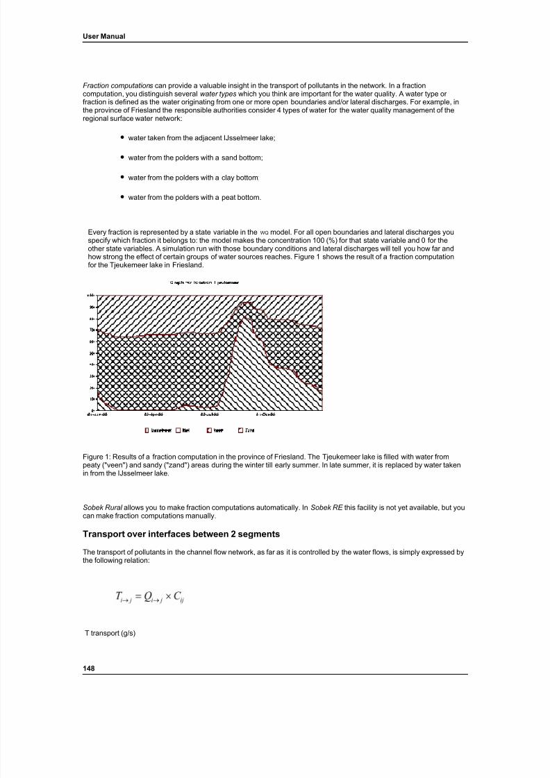
7/21/2019 SOBEK - UserManual
http://slidepdf.com/reader/full/sobek-usermanual 154/179
User Manual
Fraction computations can provide a valuable insight in the transport of pollutants in the network. In a fractioncomputation, you distinguish several water types which you think are important for the water quality. A water type or fraction is defined as the water originating from one or more open boundaries and/or lateral discharges. For example, inthe province of Friesland the responsible authorities consider 4 types of water for the water quality management of theregional surface water network:
• water taken from the adjacent IJsselmeer lake;
• water from the polders with a sand bottom;
• water from the polders with a clay bottom;
• water from the polders with a peat bottom.
Every fraction is represented by a state variable in the WQ model. For all open boundaries and lateral discharges youspecify which fraction it belongs to: the model makes the concentration 100 (%) for that state variable and 0 for theother state variables. A simulation run with those boundary conditions and lateral discharges will tell you how far andhow strong the effect of certain groups of water sources reaches. Figure 1 shows the result of a fraction computationfor the Tjeukemeer lake in Friesland.
Figure 1: Results of a fraction computation in the province of Friesland. The Tjeukemeer lake is filled with water frompeaty ("veen") and sandy ("zand") areas during the winter till early summer. In late summer, it is replaced by water takenin from the IJsselmeer lake.
Sobek Rural allows you to make fraction computations automatically. In Sobek RE this facility is not yet available, but youcan make fraction computations manually.
Transport over interfaces between 2 segments
The transport of pollutants in the channel flow network, as far as it is controlled by the water flows, is simply expressed bythe following relation:
T transport (g/s)
148
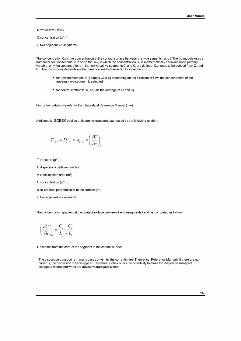
7/21/2019 SOBEK - UserManual
http://slidepdf.com/reader/full/sobek-usermanual 155/179
User Manual
Q water flow (m 3/s)
C concentration (g/m 3)
i,j two adjacent WQ-segments
The concentration C i,j is the concentration at the contact surface between the WQ-segments i and j. The WQ module uses anumerical solution technique to solve the ADV, in which the concentration C i,j is mathematically speaking not a primaryvariable: only the concentrations in the individual WQ-segments C i and C j are defined. C i,j needs to be derived from C i andC j. How this is done depends on the numerical method selected to solve the ADV:
• for upwind methods: Ci,j equals Ci or Cj depending on the direction of flow: the concentration of theupstream wq-segment is selected;
• for central methods: Ci,j equals the average of Ci and Cj.
For further details, we refer to the Theoretical Reference Manual ( TRM).
Additionally, SOBEK applies a dispersive transport, expressed by the following relation:
T transport (g/s)
D dispersion coefficient (m 2/s)
A cross section area (m 2)
C concentration (g/m 3)
n co-ordinate perpendicular to the surface (m)
i,j two adjacent WQ-segments
The concentration gradient at the contact surface between the WQ -segments i and j is computed as follows:
L distance from the core of the segment to the contact surface
The dispersive transport is in many cases driven by the currents (see Theoretical Reference Manual). If there are nocurrents, the dispersion may disappear. Therefore, Sobek offers the possibility to make the dispersive transportdisappear where and when the advective transport is zero.
149
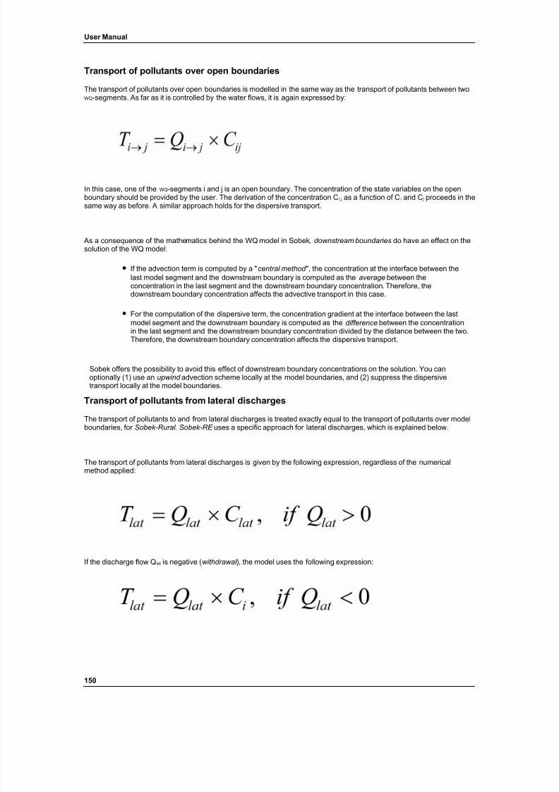
7/21/2019 SOBEK - UserManual
http://slidepdf.com/reader/full/sobek-usermanual 156/179
User Manual
Transport of pollutants over open boundaries
The transport of pollutants over open boundaries is modelled in the same way as the transport of pollutants between twoWQ -segments. As far as it is controlled by the water flows, it is again expressed by:
In this case, one of the WQ-segments i and j is an open boundary. The concentration of the state variables on the openboundary should be provided by the user. The derivation of the concentration C i,j as a function of C i and C j proceeds in thesame way as before. A similar approach holds for the dispersive transport.
As a consequence of the mathematics behind the WQ model in Sobek, downstream boundaries do have an effect on thesolution of the WQ model:
• If the advection term is computed by a " central method ", the concentration at the interface between the
last model segment and the downstream boundary is computed as the average between theconcentration in the last segment and the downstream boundary concentration. Therefore, thedownstream boundary concentration affects the advective transport in this case.
• For the computation of the dispersive term, the concentration gradient at the interface between the lastmodel segment and the downstream boundary is computed as the difference between the concentrationin the last segment and the downstream boundary concentration divided by the distance between the two.Therefore, the downstream boundary concentration affects the dispersive transport.
Sobek offers the possibility to avoid this effect of downstream boundary concentrations on the solution. You canoptionally (1) use an upwind advection scheme locally at the model boundaries, and (2) suppress the dispersivetransport locally at the model boundaries.
Transport of pollutants from lateral discharges
The transport of pollutants to and from lateral discharges is treated exactly equal to the transport of pollutants over modelboundaries, for Sobek-Rural . Sobek-RE uses a specific approach for lateral discharges, which is explained below.
The transport of pollutants from lateral discharges is given by the following expression, regardless of the numericalmethod applied:
If the discharge flow Q lat is negative ( withdrawal ), the model uses the following expression:
150
7/21/2019 SOBEK - UserManual
http://slidepdf.com/reader/full/sobek-usermanual 157/179
User Manual
where C i represents the concentration in the receiving WQ-segment. Thus, the model withdraws water with the ambientconcentrations. The lateral discharge concentrations supplied by the user are therefore neglected if the lateral dischargeflow is negative.
There is no dispersive transport related to a lateral discharge in Sobek-RE .
The model mixes the pollutants from the lateral discharge over the receiving WQ-segment. The smallest possible WQ-segment is situated between two calculation points. If a lateral discharge is situated somewhere between two calculationpoints (not possible in Sobek-Rural ), the effect of the lateral discharge will always be spread over the distance betweenthe points. So, some erroneous upstream transport of pollutants can not be avoided. If this is not acceptable, the onlypractical solution is to add more calculation points.
If a lateral discharge is situated exactly on a calculation point (obligatory in Sobek-Rural ):
• Sobek-RE divides the discharge over the grid cells upstream and downstream of the calculation point;
• Sobek-Rural puts the discharge in the reach-segment downstream of the calculation point, where thedefinition of "downstream" is evaluated based on the local and actual direction of flow.
Evaporation
In Sobek-Rural it is possible to make a boundary or lateral discharge of the type "Evaporation". This means that Sobekremoves the associated water flow from the evaluation of the substances mass balances. In other words: a boundary or lateral discharge of the type "Evaporation" does not cause a transport of pollutants. Consequently, a water balance checkin such a case would not produce correct results! In order to check the water balance the type name "Evaporation" shouldtemporarily be changed into something else.
Transport of pollutants around structures
In order to model correctly the transport of substances around structures, two aspects are important, especially relate toclosed structures: (1) to have separate WQ-segments on both sides of the structure, and (2) to make the dispersioncoefficient zero at the location of the structure.
In the present version of Sobek-Rural , the modelling of the water quality around structures may present a problem.Structure nodes are situated somewhere within a reach segment . Since the smallest possible control volume for the WQ module is a complete reach-segment, it is not possible to separate the reach-segment parts upstream and downstream of the structure over 2 WQ-segments. The complete reach-segment is considered a mixed volume in the WQ module, even if the structure is closed. We expect that this problem will not be severe. It is probably only noticeable just after a structurecloses or opens.
In the present version of Sobek-RE , it is very well possible to separate the grid cells upstream and downstream of thestructure over 2 WQ-segments. However, to make the dispersion zero locally is only possible if a separate branch iscreated for the structure, since the dispersion coefficient is necessarily constant over a branch.
Modelling the substance specific source term
The Delwaq Processes Library
So far, we have discussed the inflow of pollutants over open boundaries and via lateral discharges and the transport of pollutants within the open channel or sewer network, governed by the water flows computed by the CF module.
151
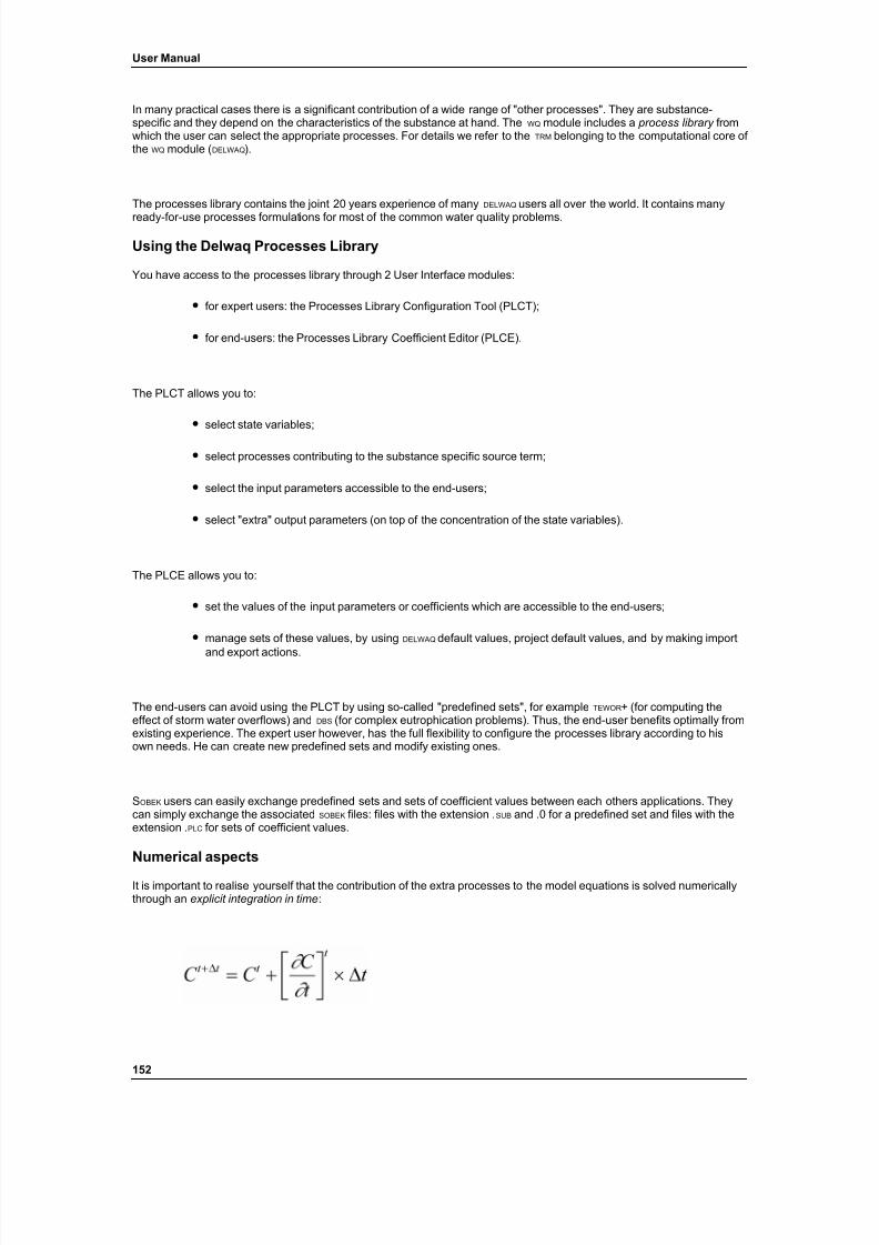
7/21/2019 SOBEK - UserManual
http://slidepdf.com/reader/full/sobek-usermanual 158/179
User Manual
In many practical cases there is a significant contribution of a wide range of "other processes". They are substance-specific and they depend on the characteristics of the substance at hand. The WQ module includes a process library fromwhich the user can select the appropriate processes. For details we refer to the TRM belonging to the computational core of the WQ module ( DELWAQ ).
The processes library contains the joint 20 years experience of many DELWAQ users all over the world. It contains many
ready-for-use processes formulations for most of the common water quality problems.
Using the Delwaq Processes Library
You have access to the processes library through 2 User Interface modules:
• for expert users: the Processes Library Configuration Tool (PLCT);
• for end-users: the Processes Library Coefficient Editor (PLCE).
The PLCT allows you to:
• select state variables;
• select processes contributing to the substance specific source term;
• select the input parameters accessible to the end-users;
• select "extra" output parameters (on top of the concentration of the state variables).
The PLCE allows you to:
• set the values of the input parameters or coefficients which are accessible to the end-users;
• manage sets of these values, by using DELWAQ default values, project default values, and by making import
and export actions.
The end-users can avoid using the PLCT by using so-called "predefined sets", for example TEWOR + (for computing theeffect of storm water overflows) and DBS (for complex eutrophication problems). Thus, the end-user benefits optimally fromexisting experience. The expert user however, has the full flexibility to configure the processes library according to hisown needs. He can create new predefined sets and modify existing ones.
S OBEK users can easily exchange predefined sets and sets of coefficient values between each others applications. Theycan simply exchange the associated SOBEK files: files with the extension . SUB and .0 for a predefined set and files with theextension . PLC for sets of coefficient values.
Numerical aspects
It is important to realise yourself that the contribution of the extra processes to the model equations is solved numericallythrough an explicit integration in time :
152
7/21/2019 SOBEK - UserManual
http://slidepdf.com/reader/full/sobek-usermanual 159/179
User Manual
where:
t time (s)
∆t time step (s)
C concentration (g/m 3)
FF forcing function(s)
MP model parameters
The new concentration value is computed starting from the old value, using the derivative of time which is multiplied withthe time step. The derivative of time is computed using the concentrations and forcing functions at the old time level . Sucha solution technique is characterised by a stability limit to the time step: if the time step is too large compared to the speedof the processes involved, the computation becomes unstable or inaccurate. For a process with a time constant k (1/d), aguideline to obtain a stable and accurate solution would be:
Thus, the quicker the process (higher value of k), the smaller the allowed time step.
Appendix G (Delwaq Processes Library)
Preface
The Sobek "Processes Editor": a flexible tool for tailor-made water quality modelling
J.A.G. van Gils
WL | Delft Hydraulics, Delft, Netherlands
ABSTRACT: Water quality modelling is practised for a wide variety of water quality problems and at different levels of complexity. WL | Delft Hydraulics’ modelling systems SOBEK (1D) and DELFT 3D (2 D/3D) use the general purpose water qualitymodel DELWAQ as the computational core for water quality simulations. The latest DELWAQ version features a ProcessesLibrary which contains software to model many relevant water quality processes to address the different types of water quality problems. The user of SOBEK and DELFT 3D has access to the processes library through a Processes Editor , which isto indicate the combination of the Processes Library Configuration Tool and the Processes Library Coefficient Editor. TheProcesses Library and the Processes Editor support the flexible set up of water quality models. The paper provides detailsabout the set-up of the Processes Library and Processes Editor and about their application. Examples are given for different problem fields and different levels of complexity.
153
7/21/2019 SOBEK - UserManual
http://slidepdf.com/reader/full/sobek-usermanual 160/179
User Manual
Introduction of Processes Library and Editor
Water quality modelling has become a widely accepted tool to support water quality pollution control and integrated water management. The purpose of such exercises is usually to find cost-effective solutions: define those strategies andmeasures which are the most beneficial for the aquatic environment against the lowest cost.
Water quality modelling is practised for a wide variety of water quality problems and at different levels of complexity.Relevant water quality problems range from the "classical" dissolved oxygen problem to complex eutrophicationphenomena or problems with pollution by toxic substances (e.g. heavy metals and pesticides). The associated water quality models vary between the simple Streeter-Phelps BOD -DO model to eutrophication models with up to 50 statevariables, representing the water column and the top sediment layers. WL | Delft Hydraulics uses the general purposewater quality modelling programme DELWAQ for the full range of applications mentioned above. This programme goes back20 years and accumulates the collective experience of WL | Delft Hydraulics’ staff over this period, plus the experience of DELWAQ users all over the world.
In most practical cases, water quality modelling is a complex task. As opposed to hydraulic modelling, water qualitymodelling is still more an "art" than a science: there is no fixed set of model equations, the required input data are many,their availability usually limited and their quality sometimes poor. During the exercise the understanding of the modeller increases, his appreciation of the problem at hand often changes and so do the model equations he wants to use. In order to perform such a complex task in an efficient way, the modeller has two wishes: (1) to profit as much as possible fromknowledge and experience gained during previous modelling exercises, and (2) to keep the full flexibility in modellingtechniques. To this end the Processes Editor and the Processes Library of DELWAQ have been designed and implemented.
Setup of Processes Library and Editor
Water Quality Modelling
The basis for water quality modelling is the well-known advection-diffusion equation. In one spatial dimension it reads:
where:
C concentration (g.m-3
)
Kx longitudinal dispersion coefficient (m 2.s -1)
S source term (g.m -3 .s -1)
t time (s)
Ux longitudinal velocity (m.s -1)
x longitudinal co-ordinate (m)
This equation can be solved for 1 state variable or substance (e.g. coliform bacteria), 2 state variables (e.g. BODO ) or manymore state variables (e.g. eutrophication). Part of the complexity of water quality modelling stems from the source term S
on the right hand side of the basic equation. This term is substance specific and it can consist of 1 up to an almost infinitenumber of sub-terms or processes . In multi-substance models, different state variables are often inter-linked through the Sterm: the degradation of BOD , for example, also consumes dissolved oxygen ( DO).
Individual processes are controlled by the participating state variables, so-called model parameters , and so-called forcing functions . Model parameters are usually scalar quantities which affect the process in question. Relevant examples arerate constants (e.g. decay rate of BOD ), temperature dependency constants and the partition coefficient for sorption of heavy metals to suspended solids. Forcing functions are external (non-modelled) quantities, usually space and/or timedependent, which affect the fate and behaviour of the state variables. Examples are meteorological quantities, such aswind velocity, solar irradiation and water temperature.
154
7/21/2019 SOBEK - UserManual
http://slidepdf.com/reader/full/sobek-usermanual 161/179
User Manual
The difference between state variables and forcing functions varies between individual models and sometimes betweensubsequent development stages of one model. For example, inorganic suspended solids can be a state variable in amodel which investigates the environmental effects of sludge dumping. However, the concentration of inorganicsuspended solids can be an external forcing function in a eutrophication model.
Processes Library
The Processes Library includes software to model many relevant water quality processes to address the different types of water quality problems mentioned above. This generic library has been composed of dedicated software made during 20years of WL | Delft Hydraulics’ research and application projects. It is regularly updated with extended or new processformulations. The present scope of the library is the following:
• microbiological pollution;
• dissolved oxygen;
• nutrients and eutrophication (simple and complex);
• heavy metals and phosphorus sorption (simple and complex);
• organic toxic substances like pesticides and PCB ’s.
In the Processes Library, a process is defined as follows: it is a physical, chemical or bio-chemical phenomenon which isresponsible for (a part of) the term S, for one or more potential state variables. The actual value of its contribution to theterm S is referred to as the process flux . The Processes Library consists of individual pieces of computer code(subroutines ), which each represent a process.
A process is defined in terms of:
• input items (state variables, model parameters, forcing functions);
• output items;
• computed fluxes;
• effect of fluxes on state variables.
This definition is kept in a process definition file (PDF ). The PDF also contains default values for the input items, if they arerelevant.
Output items play a vital role. On one hand they allow the user to monitor the correct set-up of the S term. On the other hand, an output item of one process can be an input item for another one. Thus, an inter-linked set of processes can bebuilt. An example: the process primary production has an input item light efficiency , which is computed by a separateprocess, which uses the light extinction coefficient , which is computed by yet another process.
An important feature of the Processes Library is the availability of alternative versions for clusters of processes. Typically,simple and more elaborate alternatives are available. Examples are the simple and more complex approaches for phytoplankton growth, sediment modelling and sorption of heavy metals. On a smaller scale, some processes featuredifferent alternatives: the reaeration process for example features 9 alternative formulas.
The Processes Editor is the Graphical User Interface built on the Processes Library. It facilitates the following tasks:
• selection of state variables;
• selection of processes;
• inter-linking of processes;
• accepting or overruling of available default values;
• selection of alternative processes or alternative formulas within one process;
• definition of forcing functions.
155
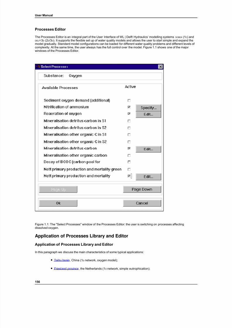
7/21/2019 SOBEK - UserManual
http://slidepdf.com/reader/full/sobek-usermanual 162/179
User Manual
Processes Editor
The Processes Editor is an integral part of the User Interface of WL | Delft Hydraulics’ modelling systems SOBEK (1D) andDELFT 3D (2D/3 D). It supports the flexible set up of water quality models and allows the user to start simple and expand themodel gradually. Standard model configurations can be loaded for different water quality problems and different levels of complexity. At the same time, the user always has the full control over the model. Figure 1.1 shows one of the major windows of the Processes Editor.
Figure 1.1: The "Select Processes" window of the Processes Editor: the user is switching on processes affectingdissolved oxygen.
Application of Processes Library and Editor
Application of Processes Library and Editor
In this paragraph we discuss the main characteristics of some typical applications:
• Taihu basin , China (1 D network, oxygen model);
• Friesland province , the Netherlands (1 D network, simple eutrophication);
156
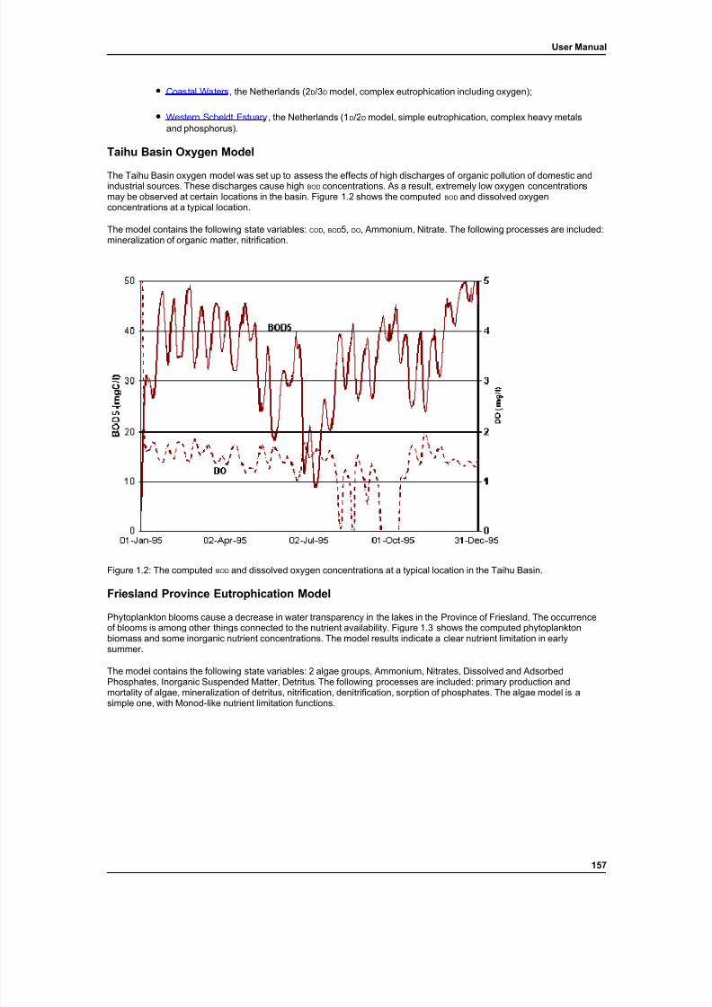
7/21/2019 SOBEK - UserManual
http://slidepdf.com/reader/full/sobek-usermanual 163/179
User Manual
• Coastal Waters , the Netherlands (2 D/3 D model, complex eutrophication including oxygen);
• Western Scheldt Estuary , the Netherlands (1 D/2D model, simple eutrophication, complex heavy metalsand phosphorus).
Taihu Basin Oxygen Model
The Taihu Basin oxygen model was set up to assess the effects of high discharges of organic pollution of domestic andindustrial sources. These discharges cause high BOD concentrations. As a result, extremely low oxygen concentrationsmay be observed at certain locations in the basin. Figure 1.2 shows the computed BOD and dissolved oxygenconcentrations at a typical location.
The model contains the following state variables: COD , BOD 5, DO , Ammonium, Nitrate. The following processes are included:mineralization of organic matter, nitrification.
Figure 1.2: The computed BOD and dissolved oxygen concentrations at a typical location in the Taihu Basin.
Friesland Province Eutrophication Model
Phytoplankton blooms cause a decrease in water transparency in the lakes in the Province of Friesland. The occurrenceof blooms is among other things connected to the nutrient availability. Figure 1.3 shows the computed phytoplanktonbiomass and some inorganic nutrient concentrations. The model results indicate a clear nutrient limitation in earlysummer.
The model contains the following state variables: 2 algae groups, Ammonium, Nitrates, Dissolved and AdsorbedPhosphates, Inorganic Suspended Matter, Detritus. The following processes are included: primary production andmortality of algae, mineralization of detritus, nitrification, denitrification, sorption of phosphates. The algae model is a
simple one, with Monod-like nutrient limitation functions.
157
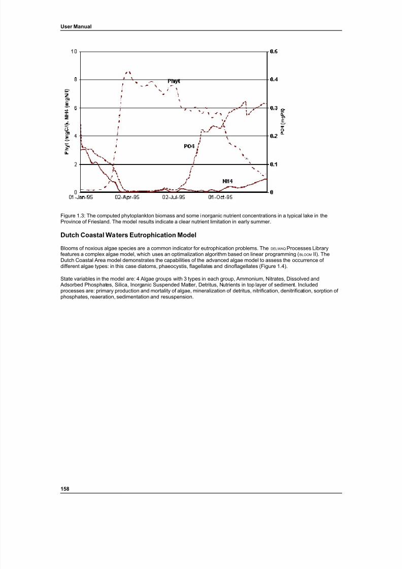
7/21/2019 SOBEK - UserManual
http://slidepdf.com/reader/full/sobek-usermanual 164/179
User Manual
Figure 1.3: The computed phytoplankton biomass and some inorganic nutrient concentrations in a typical lake in theProvince of Friesland. The model results indicate a clear nutrient limitation in early summer.
Dutch Coastal Waters Eutrophication Model
Blooms of noxious algae species are a common indicator for eutrophication problems. The DELWAQ Processes Libraryfeatures a complex algae model, which uses an optimalization algorithm based on linear programming ( BLOOM II). TheDutch Coastal Area model demonstrates the capabilities of the advanced algae model to assess the occurrence of different algae types: in this case diatoms, phaeocystis, flagellates and dinoflagellates (Figure 1.4).
State variables in the model are: 4 Algae groups with 3 types in each group, Ammonium, Nitrates, Dissolved and Adsorbed Phosphates, Silica, Inorganic Suspended Matter, Detritus, Nutrients in top layer of sediment. Includedprocesses are: primary production and mortality of algae, mineralization of detritus, nitrification, denitrification, sorption of
phosphates, reaeration, sedimentation and resuspension.
158
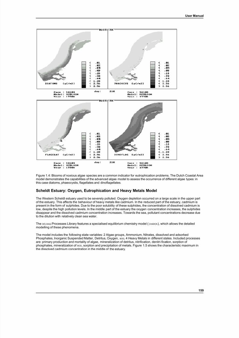
7/21/2019 SOBEK - UserManual
http://slidepdf.com/reader/full/sobek-usermanual 165/179
User Manual
Figure 1.4: Blooms of noxious algae species are a common indicator for eutrophication problems. The Dutch Coastal Areamodel demonstrates the capabilities of the advanced algae model to assess the occurrence of different algae types: inthis case diatoms, phaeocystis, flagellates and dinoflagellates.
Scheldt Estuary: Oxygen, Eutrophication and Heavy Metals Model
The Western Scheldt estuary used to be severely polluted. Oxygen depletion occurred on a large scale in the upper partof the estuary. This affects the behaviour of heavy metals like cadmium. In the reduced part of the estuary, cadmium ispresent in the form of sulphides. Due to the poor solubility of these sulphides, the concentration of dissolved cadmium islow, despite the high pollution levels. In the middle part of the estuary the oxygen concentration increases, the sulphidesdisappear and the dissolved cadmium concentration increases. Towards the sea, pollutant concentrations decrease dueto the dilution with relatively clean sea water.
The DELWAQ Processes Library features a specialised equilibrium chemistry model ( CHARON ), which allows the detailedmodelling of these phenomena.
The model includes the following state variables: 2 Algae groups, Ammonium, Nitrates, dissolved and adsorbedPhosphates, Inorganic Suspended Matter, Detritus, Oxygen, BOD , 4 Heavy Metals in different states. Included processesare: primary production and mortality of algae, mineralization of detritus, nitrification, denitri-fication, sorption of phosphates, mineralization of BOD , sorption and precipitation of metals. Figure 1.5 shows the characteristic maximum inthe dissolved cadmium concentration in the middle of the estuary.
159

7/21/2019 SOBEK - UserManual
http://slidepdf.com/reader/full/sobek-usermanual 166/179
User Manual
Figure 1.5: A characteristic maximum in the dissolved cadmium concentration in the middle of the Western Scheldtestuary.
The application of the Processes Library and Processes Editor allows the water quality expert to build on the accumulatedexperience of many years of water quality modelling. Thus the expert can improve the quality of his advises and be morecost-effective. However, the Processes Editor and Library are not a substitute for expert knowledge. They are only a toolto increase quality and efficiency.
Appendix H (Structure Control options in Sobek-RE)Structure Control Options incorporated in SOBEK River
By Thieu van Mierlo.
This is a more detailed description of the use of controllers in SOBEK RE. The following subjects are available:
General
Controlling Procedure Applied in SOBEK
Overview of Controllers Available in SOBEK
Trigger Procedure Applied in SOBEK
Overview Of Triggers Available in SOBEK
General
A distinction is to be made between a controller, a control parameter, and a controlled parameter, viz:
160
7/21/2019 SOBEK - UserManual
http://slidepdf.com/reader/full/sobek-usermanual 167/179
User Manual
1. A controller is referred to as the computational procedure in SOBEK, which facilitates the user-definedway of controlling a particular structure.
2. A control parameter refers to a parameter, which acts as the input to the controller in order to controlanother parameter, being the controlled parameter.
3. A controlled parameter refers to the parameter, which the user likes to be controlled in a specific wayduring a SOBEK computation.
Example 1:
Consider the fact that a user likes to maintain the discharge, flowing out of a small barrage constant in time bymanipulating the crest height of a weir accommodated in this barrage. For this case the user can select the intervalcontroller option in SOBEK. The crest height of the weir will be the control parameter, while the outflow discharge is thecontrolled parameter.
Example 2:
Consider a weir operated by a time controller, which maintains the user-defined time-dependent crest-levels of the weir.In this case the crest level is the controlled parameter. It will be obvious that there is no control parameter in this
example.
Following parameters of hydraulic structures can be used for controlling purposes, viz:
1. Weir: crest level can be adjusted.
2. Advanced weirs: both crest level and crest width can be adjusted.
3. General structure: crest level, crest width and gate opening can be adjusted.
4. Pump: Start- and stop water levels of a pump can be adjusted.
In SOBEK compound structures can be defined, meaning that several different type of hydraulic structures can be definednext to each other at the same location. Each member of the compound structure has its own triggers and controllers.
Controlling Procedure Applied in SOBEK
Controlling Procedure Applied in SOBEK
The procedure, applied in SOBEK, for controlling hydraulic structures can briefly be explained as follows:
• The user has to define a trigger. During a computation a trigger can either be "ON" or "OFF". In case atrigger is "ON", the corresponding controller will be activated. In case a trigger is "OFF", thecorresponding controller will be deactivated.
• A controller can be activated or de-activated by a trigger or by a combined trigger (maximum of four triggers can be combined to one combined trigger).
• In S0BEK a maximum of four controllers can be assigned to one particular hydraulic structure. It is to bementioned that SOBEK does not check for inconsistencies in the formulations of the four user-definedcontrollers.
Overview of Controllers Available in SOBEK
161
7/21/2019 SOBEK - UserManual
http://slidepdf.com/reader/full/sobek-usermanual 168/179
User Manual
Overview of Controllers Available in SOBEK
General aspects of controllers in SOBEK are:
• In case a trigger or a combined trigger is "ON", the corresponding controller will be activated, resulting inthe fact that a particular hydraulic structure will be controlled in a user-defined way.
• The controller is only activated once during a computational time step (i.e. at the beginning of a timestep execution), meaning that the value of the controlled parameter is not updated during the Newtoniteration process of solving the flow equations.
• The user has to define the control frequency, which refers to the time interval, after which the controlledparameter is to be updated again, in case the controller has not yet been de-activated. A default value for the control frequency is 1 (one) , meaning that the controlled parameter will be updated at the beginningof each and every time step for which the controller has not yet been deactivated.
Six different types of controllers can be discerned, viz:
• Time controller ,
• Relative time controller ,
• Relative from value controller ,
• Hydraulic controller ,
• Interval controller , and
• PID controller .
Controlles available in Sobek
Time controller
The time controller option in SOBEK can be used for changing the settings of a hydraulic structure (controlledparameter) during a computation.
The controlled parameter can for instance be:
• the crest level of a hydraulic structure,
• the crest width of a hydraulic structure, or
• the gate opening of a hydraulic structure
Please note that there is no control parameter in case the time controller option of SOBEK is applied.
The following input is to be specified by the user in case the time controller option in SOBEK is used, viz:
Regarding the controlled parameter
• Define whether it is the crest height, crest width or gate opening of a particular hydraulic structure.
• Specify the time-dependent values of the controlled parameter by means of a user-defined time-table.
Regarding the control parameter:
• A control parameter is not applicable, therefore no input data regarding this topic needs to be specified bythe user.
162
7/21/2019 SOBEK - UserManual
http://slidepdf.com/reader/full/sobek-usermanual 169/179
User Manual
Regarding the controller and control procedure:
• Control frequency:This defines how often the controller function should be updated. Normally this will be every time-step,but can also be an interval of more time steps. When you enter 1, the controller will be updated everytime-step; for 2 it will be updated every second time-step, and so on. Default is 1.
•Control mechanism:The procedure followed by the time controller is straightforward. Based on the computational time t,SOBEK determines in the user-defined time-table the requested value for the controlled parameter. After that SOBEK takes care that this value i s given to the controlled parameter (e.g. the crest height, the crestwidth or the gate opening of the hydraulic structure)
• Control accuracy and applicability:Using this option the user should pay much attention in specifying a realistic time-table for the controlledparameter in order to avoid instabilities in the computation. A realistic time-table for the controlledparameter means a time-table which can be met from the hydrodynamic point of view.
Relative Time Controller
Relative Time Controller
The relative time controller option in SOBEK can be applied for changing the settings of a hydraulic structure
(controlled parameter) during a computation. The relative time controller can, therefore, be referred to as an timecontroller type of controller.
The difference with the time controller option comprise of the fact that in the relative time controller option, the values for the controlled parameter have not to be specified for the entire computation time. When activated the relative timecontroller starts at the top of the user-defined time-table and from there on continues downward until the controller is de-activated by its trigger.
The controlled parameter can for instance be:
• the crest level of a hydraulic structure,
• the crest width of a hydraulic structure, or
• the gate opening of a hydraulic structure.
Please note that there is no control parameter in case the time controller option of SOBEK is applied.
The following input is to be specified by the user in case the relative time controller option in SOBEK is used, viz:
Regarding the controlled parameter:
• Define wether it is the crest height, crest width or gate opening of a particular hydraulic structure.
• Specify the relative time-dependent values of the controlled parameter by means of a user-defined timetable.
Regarding the control parameter:
• A control parameter is not applicable, therefore no input data regarding this topic needs to be specified by theuser.
Regarding the controller and control procedure:
• Control. FrequencyThis defines how often the controller function should be updated. Normally this will be every time-step, but canalso be an interval of more time steps. When you enter 1, the controller will be updated every time-step; for 2 itwill be updated every second time-step, and so on. Default is 1.
163
7/21/2019 SOBEK - UserManual
http://slidepdf.com/reader/full/sobek-usermanual 170/179
User Manual
• Control mechanism:The procedure of the relative time controller is as follows:
• When activated the controller starts at the top of the user-defined time-table and continues downward untilthe controller is de-activated by its trigger.
• When the controller reaches the end of the timetable, the value of the controlled parameter is kept constant
at the value found in the last row of the time-table.
• Control accuracy and applicability:Using this option the user should pay much attention in specifying a realistic time-table for the controlledparameter in order to avoid instabilities in the computation. In addition the value of the controlled parameter atthe moment that the controller is activated should be preferably be known in order to avoid large discontinuitiesand hence instabilities during the computation, which might even result in a termination of the program. Arealistic time-table for the controlled parameter means a time-table which can be met from the hydrodynamicpoint of view.When the trigger is switched off and at a later time switched on again, the controlled parameter will get thevalue at the current time.
Relative from Value Controller
Relative from Value Controller
The relative from value controller option in SOBEK can be used for changing the settings of a hydraulic structure(controlled parameter) during a computation. The relative from value controller can, therefore, be referred to as an timecontroller type of controller.
As for the relative time controller option in the relative from value controlled option the values for the controlled parameter have not to be specified for the entire computation time.
The difference with the relative time controller option comprises of the fact that the relative from value controller option isusually applied when the actual values of the controlled parameter are unknown at the moment in which the relative fromvalue controller is activated. Therefore, when activated the relative from value controller first determines the actual valueof the controlled parameter. After that the relative from value controller starts in the user-defined time-table at the actualvalue of the controlled parameter and continues downwards from this value onwards. In this way possible largediscontinuities in the value of the controlled parameter are avoided and hence instabilities in SOBEK computations,leading to the termination of the program.
The following input is to be specified by the user in case the relative from value controller option in SOBEK is used, viz:
Regarding the controlled parameter:
• Define wether it is the crest height, crest width or gate opening of a particular hydraulic structure.
• Specify the relative time-dependent values of the controlled parameter by means of a user-definedtimetable.
Regarding the control parameter:
• A control parameter is not applicable, therefore no input data regarding this topic needs to be specified by
the user.
Regarding the controller and control procedure:
• Control frequency:This defines how often the controller function should be updated. Normally this will be every time-step,but can also be an interval of more time steps. When you enter 1, the controller will be updated everytime-step; for 2 it will be updated every second time-step, and so on. Default is 1.
• Control mechanism:The procedure of the relative from value controller is as follows:
164
7/21/2019 SOBEK - UserManual
http://slidepdf.com/reader/full/sobek-usermanual 171/179
User Manual
• When activated the controller first determines the actual value of the controlled parameter. After that thecontroller searches for the line in the user-defined time-table, which has the same value as the actual valueof the controlled parameter. For the time that the controller remains activated, the controller movesdownward in the time-table from this line onwards.
• When the controller reaches the end of the timetable, the value of the controlled parameter is kept constantat the value found in the last row of the time-table.
• Control accuracy and applicability:Using this option the user should pay much attention in specifying a realistic time-table for the controlledparameter in order to avoid instabilities in the computation. A realistic time-table for the controlledparameter means a time-table which can be met from the hydrodynamic point of view.
Hydraulic controller
Hydraulic controller
The hydraulic controller option in SOBEK can be used to operate a hydraulic structure (i.e. the controlled parameter)based on the actual value of a specified hydraulic parameter (i.e. the control parameter).
The controlled parameter can for instance be:
• the crest level of a hydraulic structure,
• the crest width of a hydraulic structure, or
• the gate opening of a hydraulic structure
The control parameter can be either:
• the actual value of a water level at a specific location,
• the actual value of the averaged flow velocity in the total flow section at a specific location,
• the actual direction of the flow at a specific location,
• the actual value of a discharge at a specific location (or the sum of the actual values of discharge over amaximum of five locations),
• the actual head-difference over a hydraulic structure. The head-difference of another structure than thecontrolled structure can be used.
• the actual pressure-difference over a hydraulic structure. The pressure-difference of another structurethan the controlled structure can be used.
The following input is to be specified by the user in case the Hydraulic controller in SOBEK is used, viz:
Regarding the controlled parameter.
• Define whether it is the crest height, crest width or gate opening of a particular hydraulic structure.
• Note that the requested values for the controlled parameter are determined from the controller-function,which is discussed in point 4.c of this paragraph. It is, therefore, not necessary to specify the minimumand maximum value of the control parameter as well as the maximum possible adjustment of the controlparameter over a time step
Regarding the control parameter.
165
7/21/2019 SOBEK - UserManual
http://slidepdf.com/reader/full/sobek-usermanual 172/179
User Manual
• Definition of the type of hydraulic control parameter (i.e. whether it is a water-level, a velocity, the flowdirection, a discharge, a head difference over a structure, or a pressure difference over a structure) .
• Definition of the location of the hydraulic control parameter (i.e. either the specific location (in case of awater-level, a velocity, the flow direction or discharge) or the concerning structure in case of a headdifference or pressure difference).
• Definition of the controller-function (or controller table) for the specified hydraulic control parameter. Thecontroller-function contains the relation between the actual value of the hydraulic control parameter andthe by the user requested value of the controlled parameter (e.g. the crest height, the crest width or thegate opening of the controlled hydraulic structure).
Regarding the controller and control procedure.
• Control frequency:This defines how often the controller function should be updated. Normally this will be every time-step,but can also be an interval of more time steps. When you enter 1, the controller will be updated everytime-step; for 2 it will be updated every second time-step, and so on. Default is 1.
• Control mechanism:The procedure followed by the Hydraulic controller is straightforward. First, the actual value of thehydraulic controller for t = t is determined. Next the value of controlled parameter (e.g. the crest height,crest width or gate opening of the hydraulic structure) is obtained by interpolation in the user-definedcontroller table. Finally SOBEK adjusts the actual value at t = t + dt of the crest height, crest width or gateopening of the hydraulic structure in accordance with the findings of the interpolation in the controller table.
• Control accuracy and applicability:Using this option the user should pay much attention in specifying a realistic controller-function (i.e. therelation between the value of the control parameter and the requested value of the controlled parameter)in order to avoid instabilities in the computation. A realistic controller-function means a function which canbe met from the hydrodynamic point of view.
Interval controller
Interval controller
The interval controller can be used to operate a hydraulic structure (i.e. the control parameter) in such way that user-specified values of a hydraulic parameter (i.e. controlled parameter) are maintained.
The controlled parameter can be either:
• a water level at a specific location, or
• a discharge at a specific in the model.
Note: The location of the to be controlled parameter should be under the control range of the concerning hydraulicstructure.
The control parameter can for instance be either:
• the crest level of a hydraulic structure,
• the crest width of a hydraulic structure, or
• the gate opening of a hydraulic structure
The following input is to be specified by the user in case the Interval controller option in SOBEK is used, viz:
166
7/21/2019 SOBEK - UserManual
http://slidepdf.com/reader/full/sobek-usermanual 173/179
User Manual
Regarding the controlled parameter:
• Definition of the controlled parameter (i.e. water level or discharge at a particular location in the model).
• Setpoints for the controlled parameter. These are in fact the user-defined values for the controlledparameter. There are two possibilities in SOBEK, viz:
• a constant water level or discharge, or
• a time-dependent water level or discharge, defined by means of a table.
• Definition of the dead band type. on basis of the specified dead band type, SOBEK determines whether the value of the controller (v.) (e.g. crest height, crest width or gate opening of the hydraulic structure) areto be adjusted. The following dead band types are available in SOBEK, viz:
• A constant dead band value (D), or.
• A dead band (D) as percentage of the discharge.In this case except for the percentage, the minimum and maximum dead band values are to be specifiedas well.
Regarding the control parameter:
• Define wether it is the crest height, crest width or gate opening of a particular hydraulic structure.
• The minimum and maximum values of the control parameter (e.g. minimum and maximum crest width.
• Definition of the control interval (dv s ) , which refers to the user-defined change in the value of the controlparameter over 1 (one) time step. The reason why the user has to define a control interval (dv s ) is the factthat in reality it takes time to adjust the crest height, crest width or gate opening of hydraulic structure. Inpractical situations there is a limit to the change in the value of the control parameter over a time step. InSOBEK two types of control interval can be defined, viz:
• fixed control interval,meaning that if required the value of the control parameter can be adjusted with a constant value only (for instance 0. 1 m' in case of a gated structure).
• variable control interval,meaning that if required the value of the control parameter can be adjusted by the product of the actualtime step dt times the user-defined adaptation velocity (v). For instance in case of a gated structure theadaptation velocity (v) might be 0.2 m 2/hour, meaning that over a time step dt = 0.5 hour, the change invalue of the control parameter (if activated by its trigger) will be 0.2 * 0.5 = 0.1 m 2)
Regarding the controller and control procedure:
• The control frequency:which refers to the time interval after which SOBEK updates the value of the to-be-controlled parameter incase the controller has not yet been de-activated by its trigger or combined trigger (see also point 3 under General aspects of controllers),
167
7/21/2019 SOBEK - UserManual
http://slidepdf.com/reader/full/sobek-usermanual 174/179
User Manual
• The control mechanism:SOBEK applies the following algorithm for determining whether the value of the control parameter (v.) isto be updated, viz:if -0.5 D < e < +0.5 D then V s = Vs , old
if e < -0.5 D then V s = V s , old + dv s
if e > +0.5 D then v s , = V s, old - dv s
in which:D = dead band (in [m] in case of water level, and in [m 3/s]
in case of discharge),e = deviation of the controlled parameter
= setpoint - actual value of the controlled parameter)dv s = control interval (fixed value or computed by dv s = v * dt,
in which v = adaptation velocity)vs old = value of the control parameter in the previous time step.
• Controller accuracy and applicability:The interval controller is not a very advanced type of controller. It is for instance, sensitive to instabilities,in particular if the adaptation velocity, control frequency or dead band are not selected properly. Also thecontrol history (before the last time step is not taking into account to determine the control parameter.
PID Controller
PID Controller
As for the interval controller, the PID controller, can be used to operate a hydraulic structure (i.e. the control parameter)in such way (i.e. by adjusting its crest level, crest width or gate opening) , that user-specified values of a hydraulicparameter (i.e. controlled parameter) are maintained.The difference with the interval controller option comprises of the fact that the PID controller option does take the controlhistory into account.
The controlled parameter can be either:
• a water level at a specific location, or
• a discharge at a specific location in the model.
Note: The location of the to be controlled parameter should be under the control range of the concerning hydraulicstructure.
The control parameter can for instance be either:
• the crest level of a hydraulic structure,
• the crest ,width of a hydraulic structure, or
• the gate opening of a hydraulic structure
The following input is to be specified by the user in case the PID controller option in SOBEK is used, viz:
Regarding controlled parameter:
• Definition of the controlled parameter (i.e. water level or discharge at a particular Iocation in the model).
• Setpoints for the controlled parameter. These are in fact the user-defined values for the controlledparameter. There are two possibilities in SOBEK, viz:
• a constant water level or discharge, or
• a time-dependent water level or discharge, defined by means of a table.
168
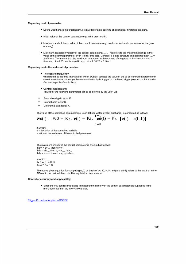
7/21/2019 SOBEK - UserManual
http://slidepdf.com/reader/full/sobek-usermanual 175/179
User Manual
Regarding control parameter:
• Define weather it is the crest height, crest width or gate opening of a particular hydraulic structure.
• Initial value of the control parameter (e.g. initial crest width).
• Maximum and minimum value of the control parameter (e.g. maximum and minimum values for the gate
opening) .
• Maximum adaptation velocity of the control parameter (v max ). This refers to the maximum change in thevalue of the control parameter over 1 (one) time step. Consider a gated structure and assume that v max =2 m 2/hour. This means that the maximum adaptation in the opening of the gates of the structure over atime step dt = 0.25 hour is equal to v max . dt = 2 * 0.25 = 0. 5 m 2.
Regarding controller and control procedure:
• The control frequency,which refers to the time interval after which SOBEK updates the value of the to-be-controlled parameter incase the controller has not yet been de-activated by its trigger or combined trigger (see also point 3 under General aspects of controllers),
• Control mechanism:
Values for the following parameters are to be defined by the user, viz:
• Proportional gain factor K p.
• Integral gain factor K i.
• Differential gain factor K d.
The value of the controlled parameter (i.e. user-defined water level of discharge) is computed as follows:
in which:e = deviation of the controlled variable= setpoint - actual value of the controlled parameter
The maximum change of the control parameter is checked as follows:if |dv| < dv max then vs = v s
if dv < -dv max then v s = v s, old - dv max
if dv > +dv max then v s = v s, old + dv max
in which:dv = v s(t) - v s(t-1)dv max = v max * dt
The above given equation for computing w s(t) on basis of w 0, Kp, Ki, Kd, e(t) and e(t-1), refers to the fact that in thePID controller method the control history is taken into account.
Controller accuracy and applicability:
• Since the PID controller is taking into account the history of the control parameter it is supposed to bemore accurate than the interval controller.
Trigger Procedure Applied in SOBEK
169

7/21/2019 SOBEK - UserManual
http://slidepdf.com/reader/full/sobek-usermanual 176/179
User Manual
Triggers in Sobek
Trigger Procedure Applied in SOBEK
In general the procedure is as follows:
Depending on the status ("ON or "OFF") of a particular trigger, the corresponding controller will be activated or de-
activated.
Up to four triggers can be combined to activate a controller. When the user specifies more than one trigger, he mustspecify how the triggers work together by specifying the relation-ship between the triggers with logical AND-ORstatements. Evaluation of AND-OR statements are according to the usual logical rules. This means that AND statementsare evaluated before OR statements.
This results in the following:
• The combination of triggers 'trig1 and trig2', 'trig12', is evaluated as follows:if trig1 ON and trig2 ON thentrig12 ON
elsetrig12 OFF.
• The combination of triggers 'trig1 or trig2', 'trig12', is evaluated as follows:if trig1 ON or trig2 ON thentrig12 is ONelsetrig12 is OFF.
• The combination of triggers 'trig1 and trig2 and trig3', 'trig123', is evaluated as follows:if 'trig1 and trig2' ON and trig3 ON thentrig123 ONelsetrig123 OFF.
• The combination of triggers 'trig1 and trig2 or trig3', 'trig123', is evaluated as follows:if 'trig1 and trig2' ON or trig3 ON thentrig123 ONelsetrig123 OFF.
• The combination of 'trig1 or trig2 and trig3', 'trig123', is evaluated as follows:if trig1 ON or 'trig2 and trig3' ON thentrig123 ONelsetrig123 OFF.
Overview Of Triggers Available in SOBEK
170
7/21/2019 SOBEK - UserManual
http://slidepdf.com/reader/full/sobek-usermanual 177/179
Index A
About the Case Manager.............................................12
Activating a task...........................................................17
Additional functions on task blocks..............................17 Advanced Weir Description......................................... 43
Analysis of results.................................... ...................... 7
Application of Processes Library and Editor..............156 B
Basic schematisation elements................................. 146
Bed frictionWF............................................................. 54
Boundary conditions water flow................................... 56
Branches..................................... ............................ ..... 35
Buttons.......................... ............................ ................... 25 C
Colours.........................................................................16 Conditions.................................. ............................ 55, 93
Conditions salt............................................................. 57
Conditions sediment/morphology................................ 58
Conditions water quality...............................................59
Control volumes..................................... .................... 146
Controllers....................................................................49
Controlling Procedure Applied in SOBEK..................161
Conversion of Models (Step A)..................................141
Conversion of Models (Step B)..................................142
Cross sections............................................................. 85
Cross-Section Description........................................... 38
Cross-section placement.................................... ......... 41
Cross-Sections.............................................................38 D
Data fields.................................. ............................. ..... 28
Database Structure Description...................................45
Default values....................................... ....................... 30
Descriptions of windows........................................ ...... 30
Directory Structure................................... .................. 100
Discharge at branches.................................................56
Dispersion....................................... ............................ . 63
Dredging optimization............................... ................... 77
Dutch Coastal Waters Eutrophication Model.............158 E
Evaporation................................................................151
Extra Processes...........................................................22
Extra resistance.......................................... ................. 55 F
FLEXlm on Windows-95............................................ 100
FLEXlm on Windows-NT 4.0..................................... 101
Flood risk..................................................................... 78
Flow module messages.......................................... ... 128 Formats........................................................................29
Fraction computations............................................... 147
Friction................................ ............................. ...... 54, 92
Friesland Province Eutrophication Model..................157 G
General.................................... .............. 76, 79, 143, 160
General Structure Description..................................... 44
Graded sediment messages......................................135
Grid definition.........................................................64, 97
Grid points....................................................................64
Groundwater........................................ ........................ 74
H
Hardware requirements........................................ ......... 3
Horizontal water surface......................................... ..... 79
How is SOBEK organized?............................................1
How to combine two schematisations......................... 76
How to cut a schematisation........................................75
How to use this manual?............................................... 3
Hydraulic controller..................................... ............... 165 I
Import/Export of files..................................................136
Important windows........................................... ............ 29
Importing cross section..............................................138 Importing Water Quality Conditions...........................140
Initial conditions.................................... ................. 61, 97
Insensitive buttons and data fields.............................. 29
Installation on pc........................................................100
Integrated modelling of Channel Flow and Water Quality................................................................... 145
Interval controller....................................................... 166
Introduction.................................... ............................ .... 1
Introduction cutting and combining schematisations...75
Introduction of Processes Library and Editor......... ... 154
Introduction on windows......................................... ..... 24
J
Join of nodes................................................................34 K
Key shortcuts for buttons.......................... ................... 25 L
171
7/21/2019 SOBEK - UserManual
http://slidepdf.com/reader/full/sobek-usermanual 178/179
User Manual
Layers.......................................................................... 32
Layout of windows....................................................... 25
Lists..............................................................................28
LMTools Utility........................................................... 103
Low water.....................................................................78 M
Main module messages.............................................126
Making calculations......................................................75
Mass balance for pollutants................................. ...... 144
Messages computational core................................... 126
Messages User Interface 0 - 999.............................. 103
Messages User Interface 1000 - 1999...................... 104
Messages User Interface 10000 - 10999..................109
Messages User Interface 11000 - 11999..................109
Messages User Interface 12000 - 12999..................110
Messages User Interface 13000 - 13999..................111
Messages User Interface 14000 - 14999..................112
Messages User Interface 15000 - 15999..................112 Messages User Interface 16000 - 16999..................112
Messages User Interface 17000 - 17999..................112
Messages User Interface 18000 - 18999..................113
Messages User Interface 19000 - 19999..................123
Messages User Interface 2000 - 2999...................... 105
Messages User Interface 20000 - 20999..................124
Messages User Interface 21000 - 21999..................124
Messages User Interface 22000 - 22999..................125
Messages User Interface 23000 - 23999..................125
Messages User Interface 24000 - 24999..................125
Messages User Interface 25000 - 25999..................125
Messages User Interface 3000 - 3999...................... 107
Messages User Interface 4000 - 4999...................... 108
Messages User Interface 5000 - 5999...................... 108
Messages User Interface 6000 - 6999...................... 108
Messages User Interface 7000 - 7999...................... 109
Messages User Interface 8000 - 8999...................... 109
Messages User Interface 9000 - 9999...................... 109
Meteo data.............................. ............................ ......... 62
Model Attributes............................ ............................ ... 31
Modelling with SOBEK-RE............................................ 7
Morphodynamics..........................................................61
Morphology module messages..................................133 N
Nodes...........................................................................34
Numerical aspects..................................................... 152
Numerical parameters................................................. 68 O
One-dimensional..........................................................79
Output f(t).....................................................................73
Output f(x)...................................... ............................ .. 71
Overview of Controllers Available in SOBEK............162
Overview of input items............................................. 145 P
PID Controller............................................................ 168
Processes Editor................................................153, 156
Processes Library....................................... ............... 155
Processes Library Coefficient Editor........................... 22
Processes Library Configuration Tool......................... 17
Product support..............................................................3
Project management options.................................... ... 13
Projects and cases.......................................................12
Pump Description.........................................................45 R
Reading tables from ASCII file................................... 137
Regime changes..................................... ..................... 78 Relative from Value Controller...................................164
Relative Time Controller....................................... ..... 163
Restart of model calculation...................................... 142
River bend cut-offs.......................................................77
River training................................................................77
Run time data.........................................................66, 98 S
172
7/21/2019 SOBEK - UserManual
http://slidepdf.com/reader/full/sobek-usermanual 179/179
Index
Salt........................ ............................. .......................... 61
Salt intrusion module messages................................131
Saving the Configuration............................................. 22
Scheldt Estuary................................................................Oxygen.........................................................................
Eutrophication and Heavy Metals Model.........159
Sediment transport module messages...................... 132
Selection of ............................ ............................ ......... 18
Selection of Water Quality Processes Affecting the State variables.........................................................19
Service lmgrd.exe on Windows-NT 4.0..................... 101
Setting up of the model............................................4, 80
Simulations.................................................................... 6
SOBEK Messages....................................... .............. 103
sobek-model window................................................... 30
Software authorization....................................... ........ 100
Specifying or Editing a Process................................... 20
Splitting of a branch...................................... ............... 37
Startup directory related to 'Import/export files'.........100 Structure Control Options incorporated in SOBEK River
...............................................................................160
Structure description...................................... .............. 42
Structure Placement 48
Tables.......................................................................... 28
Tables with header from ASCII file............................ 137
Taihu Basin Oxygen Model........................................157
The Delwaq Processes Library..................................151
The Modelling Tasks....................................................16
The Selection of Active Substance Groups.................17
The SOBEK manuals.....................................................2
The SOBEK user........................................................... 3
Time controller..................................... ...................... 162
Time parameters..........................................................67
To import your converted model in SOBEK 2...........142
Topography............................................................33, 82
Transport formula.........................................................74
Transport of pollutants around structures..................151
Transport of pollutants from lateral discharges.........150
Transport of pollutants over open boundaries...........150
Transport over interfaces between 2 segments........148
Trigger Procedure Applied in SOBEK....................... 170
Triggers........................................................................53 U
Using the Delwaq Processes Library.........................152 W


