Soc. Stats Reading Group Four: SensitivityAnalysis

Rebecca Johnson

October 27th, 2016

1 / 37

Purpose of sensitivity analysis, to deal withconversations like these...

I You: Here are the results of my matching (or insert other methodfor causal inference with observational data that relies on someform of ignorability assumption) analysis showing that becomingunemployed causes a higher likelihood of opioid use

I Your skeptical adviser: when estimating your propensity score,did you include a measure of whether the person worked in amanual occupation on the losing end of skill-based technologicalchange?

I You: Of course!I Your skeptical adviser: what about a measure of a person’s

(pre-treatment) degree of existential suffering?I You: I think that’s impossible to observe or measure...I Your skeptical adviser: well how large would a difference in

inherent potential for opioid use among those more likely tobecome unemployed need to be to bias your results? Whenwould it lead you to find that becoming unemployed causes alower likelihood of opioid use?

I You: I have no idea...I guess I need to learn about sensitivityanalysis...

2 / 37

In diagram form

New unemployment Opioid use

Pre-treatmentexistentialsuffering

Previous workin manufacturing

3 / 37

Outline

I Blackwell1. Review of causal quantities of interest in potential outcomes

framework2. Brief diversion to Rosenbaum (2002) to build intuition about

purpose behind sensitivity analysis3. Blackwell’s approach: ”de-confound” the dependent variable using

a confounding function4. Illustrate approach with (relatively) basic case5. Focus on three extensions of basic case:

5.1 Change confounding function from one-sided bias to alignment bias5.2 Re-parametrize confounding function to express magnitude of

confounding in terms of variation in R2 rather than difference in meaninherent potential outcomes between treatment and control (α)

5.3 Going from static, cross-sectional treatment assignment to treatmentsover time (dynamic case)

I Throughout, briefly contextualize with other approachesdiscussed in Morgan and Winship

4 / 37

Causal quantities of interest and underpinningassumptions

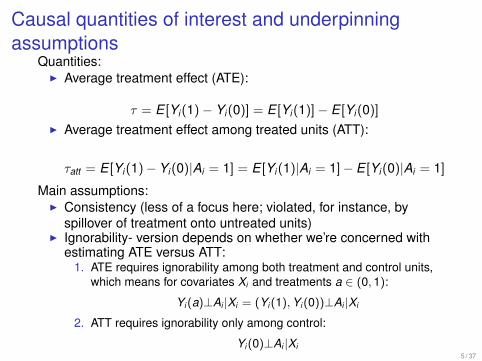
Quantities:I Average treatment effect (ATE):

τ = E [Yi (1)− Yi (0)] = E [Yi (1)]− E [Yi (0)]

I Average treatment effect among treated units (ATT):

τatt = E [Yi (1)−Yi (0)|Ai = 1] = E [Yi (1)|Ai = 1]−E [Yi (0)|Ai = 1]

Main assumptions:I Consistency (less of a focus here; violated, for instance, by

spillover of treatment onto untreated units)I Ignorability- version depends on whether we’re concerned with

estimating ATE versus ATT:1. ATE requires ignorability among both treatment and control units,

which means for covariates Xi and treatments a ∈ (0, 1):

Yi (a)⊥Ai |Xi = (Yi (1),Yi (0))⊥Ai |Xi

2. ATT requires ignorability only among control:

Yi (0)⊥Ai |Xi5 / 37

Your adviser again...

(Yi (1),Yi (0))⊥Ai |Xi

1. To satisfy above assumption, can keep on adding Xi to conditionon (while paying attention to post-treatment issues discussed inweek 1), but in observational data, there will always remainunobserved confounders correlated with both treatment statusand potential outcomes (e.g., your adviser’s comment aboutexistential suffering)

2. Sensitivity analysis: more systematically explore how thecorrelation between a unit’s probability of receiving treatment andthat unit’s potential outcomes affects magnitude and direction ofestimated treatment effect

3. What’s up next:3.1 More in-depth review of Rosenbaum (2002) than in Blackwell.

Why? Still common form of sensitivity analysis, and also gesturesat approach of modeling selection into treatment

3.2 Blackwell article

6 / 37

More background on Rosenbaum (2002)Illustrating with unemployment and opioid example:1

1. πi = Pr(Ai = 1)); 1− πi = Pr(Ai = 0); Xi are observed covariates2. Imagine Bob and Jim, where XBob = XJim (e.g., same manufacturing job,

same age, same observed disability status). Bob and Jim’s odds oftreatment (becoming unemployed) are:

OddsBob =πBob

1− πBob

OddsJim =πJim

1− πJim

3. The sensitivity parameter, Γ, is the odds ratio of these two probabilitiesof treatment, or the odds of Bob being unemployed over the odds ofidentical observed covariate Jim being unemployed:

Γ =

πBob1−πBobπJim

1−πJim

=OddsBob

OddsJim

4. While for Blackwell q(a, x) = 0 is case where we assume ignorabilityassumption is satisfied, for Rosenbaum, the case where the true valueof Γ = 1 is case where ignorability is satisfied (note that the observedvalue of Γ will always be 1 for two obs. with same observed covariatessince all we have are these observed covars to calculate the OR)

1Credit to Bertolli (2013) for helpful slides on Rosenbaum bounds7 / 37

More background on Rosenbaum continuedBasic procedure - engage in a thought experiment where we see howchanging Γ to reflect different magnitudes of confounding byunobserved variables affects results:

1. Choose range of Γ that represent worst case scenarios ofdifferent odds of Bob versus Jim becoming treated (unemployed)despite same observed covariates (e.g., if you think odds mightonly differ slightly, so πBob and πJim, though not equal, are withinthe range of 0.33 to 0.66, can calculate Γ range as follows):1.1 Lower bound: 0.33

1−0.33 = 0.51.2 Upper bound: 0.66

1−0.66 = 21.3 0.5 ≤ Γ ≤ 2 (no individual is more than twice as likely than

someone with same covariates to become unemployed)

2. Increment through different values of Γ in that range to see howsignificance and size of treatment effect changes; estimates forhow these quantities change is based on exact test thatcorresponds to nature of dependent variable2.1 Binary dependent variable: McNemar’s exact test2.2 Continuous dependent variable: Wilcoxon signed rank test for p

value and Hodges-Lehmann for point estimate

8 / 37

Illustrating with binary treatment exampleOutcomes for matched pairs:

EmployedOpioid No opioid

Unemployed Opiod 10 b = 50No opioid c = 20 140

I If Γ = 1 (so assume individuals with same observed covariateshave same probability of employed and unemployed), thenMcNemar’s exact p-value is, where n = b + c

2 ∗n∑

i=b

(ni

)0.5i 0.5n−i ≈ 0.00044

I When you increase Γ, the probabilities in red above are no longer0.5 (become: π = Γ

1+Γ and 1− π) and p-value increasesI Putting into code (mcn.exact.p finds the non-summation part of

above expression):

9 / 37

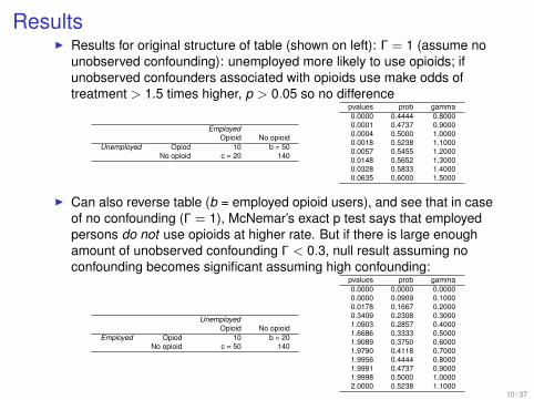
ResultsI Results for original structure of table (shown on left): Γ = 1 (assume no

unobserved confounding): unemployed more likely to use opioids; ifunobserved confounders associated with opioids use make odds oftreatment > 1.5 times higher, p > 0.05 so no difference

EmployedOpioid No opioid

Unemployed Opiod 10 b = 50No opioid c = 20 140

pvalues prob gamma0.0000 0.4444 0.80000.0001 0.4737 0.90000.0004 0.5000 1.00000.0018 0.5238 1.10000.0057 0.5455 1.20000.0148 0.5652 1.30000.0328 0.5833 1.40000.0635 0.6000 1.5000

I Can also reverse table (b = employed opioid users), and see that in caseof no confounding (Γ = 1), McNemar’s exact p test says that employedpersons do not use opioids at higher rate. But if there is large enoughamount of unobserved confounding Γ < 0.3, null result assuming noconfounding becomes significant assuming high confounding:

UnemployedOpioid No opioid

Employed Opiod 10 b = 20No opioid c = 50 140

pvalues prob gamma0.0000 0.0000 0.00000.0000 0.0909 0.10000.0178 0.1667 0.20000.3409 0.2308 0.30001.0903 0.2857 0.40001.6686 0.3333 0.50001.9089 0.3750 0.60001.9790 0.4118 0.70001.9956 0.4444 0.80001.9991 0.4737 0.90001.9998 0.5000 1.00002.0000 0.5238 1.1000

10 / 37

From Rosenbaum to Blackwell

I Takeaway from Rosenbaum:I The case where two persons with same observed covariates have

same odds of treatment is a special case; in that special case,Γ = 1

I We can explore the effect of deviations from that special case byseeing how our results change when two persons with the sameobserved covariates have different odds of treatment (Γ 6= 1)

I What does Blackwell’s approach have in common? Ignorabilityassumption on which estimates rest is a special case; explorewhether and how results change when we move away from thatspecial case

11 / 37

From Rosenbaum to Blackwell

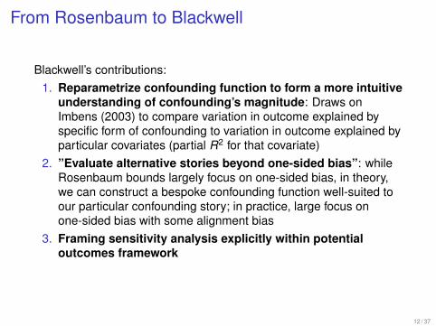
Blackwell’s contributions:1. Reparametrize confounding function to form a more intuitive

understanding of confounding’s magnitude: Draws onImbens (2003) to compare variation in outcome explained byspecific form of confounding to variation in outcome explained byparticular covariates (partial R2 for that covariate)

2. ”Evaluate alternative stories beyond one-sided bias”: whileRosenbaum bounds largely focus on one-sided bias, in theory,we can construct a bespoke confounding function well-suited toour particular confounding story; in practice, large focus onone-sided bias with some alignment bias

3. Framing sensitivity analysis explicitly within potentialoutcomes framework

12 / 37

Blackwell: the confounding functionI General form:

q(a, x) = E [Yi (A)|Ai = a,Xi = x ]− E [Yi (A)|Ai = 1− a,Xi = x ]

I Single-parameter version (equation 5):

q(a, x ;α) = E [Yi (A)|Ai = a,Xi = x ]−E [Yi (A)|Ai = 1−a,Xi = x ] = α

I One-sided bias (equation 6):

q(a, x ;α) = α(2a− 1)

I One-sided bias for treatment versus control:

q(1, x ;α) = α

q(0, x ;α) = −α

I More analytics

13 / 37

Directions of α for examples

Using the one-sided bias function (reverse italicized for α < 0)

Example α > 0; Counfounders mean...Ai = 1= unemp. Higher potential likelihood of opioid useYi (a) = opioid use among those with higher prob. of unemp.

Ai = 1 = job-training (JT) Higher potential earnings amongYi (a) = earnings among those with higher prob. of

participating in JT

Ai = 1 = fem. judge Higher potential likelihood of voting liberalon panel; among those with higher probabilityYi (a) = liberal vote of being in panel with a female

Ai = 1 = neg. campaign Higher potential turnout amongYi (a) = turnout campaigns with higher prob. of going negative

14 / 37

Once we have the confounding function, we use it to”de-confound” each observation’s observed outcome

1. Begin with each individual’s observed outcome Yi

2. Create a confounding-adjusted outcome:

Y qi = Yi − q(Ai ,Xi )Pr [1− Ai |Xi ]

3. Example with snapshot of LaLonde data and treatmentprediction equation accounting for degree status, past earnings,age, etc. and where α = 500 v. α = 2000, and adjust =q(a, x)Pr(1− Ai |Xi )

id no ai Pr(Ai Pr(1− Ai |Xi ) yi adjust yqi adjust yq

ideg. = 1) α = 500 α = 500 α = 2000 α = 2000

1 0 1 0.66 0.34 0 169 -169 676 -6762 1 1 0.36 0.64 4666 319 4348 1275 33913 1 0 0.36 0.36 445 -181 627 -725 11704 0 0 0.58 0.58 12384 -289 12673 -1156 13539

15 / 37

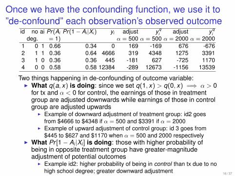
Once we have the confounding function, we use it to”de-confound” each observation’s observed outcome

id no ai Pr(Ai Pr(1− Ai |Xi ) yi adjust yqi adjust yq

ideg. = 1) α = 500 α = 500 α = 2000 α = 2000

1 0 1 0.66 0.34 0 169 -169 676 -6762 1 1 0.36 0.64 4666 319 4348 1275 33913 1 0 0.36 0.36 445 -181 627 -725 11704 0 0 0.58 0.58 12384 -289 12673 -1156 13539

Two things happening in de-confounding of outcome variable:I What q(a, x) is doing: since we set q(1, x) > q(0, x) =⇒ α > 0

for tx and α < 0 for control, the earnings of those in treatmentgroup are adjusted downwards while earnings of those in controlgroup are adjusted upwards

I Example of downward adjustment of treatment group: id2 goesfrom $4666 to $4348 if α = 500 and $3391 if α = 2000

I Example of upward adjustment of control group: id 3 goes from$445 to $627 and $1170 when α = 500 and 2000 respectively

I What Pr [1− Ai |Xi ] is doing: those with higher probability ofbeing in opposite treatment group have greater-magnitudeadjustment of potential outcomes

I Example id2: higher probability of being in control than tx due to nohigh school degree; greater downward adjustment 16 / 37

More intuition behind role of Pr(1− Ai |X ) inadjustment

I Focus on id1 and id2:id no ai Pr(Ai Pr(1− Ai |Xi )

deg. = 1)1 0 1 0.66 0.342 1 1 0.36 0.64

I One (heuristic), way to think about id2s larger adjustment is tothink about a person’s probability of treatment being partitionedinto Pr(Ai = 1|observedi ) + Pr(Ai = 1|unobservedi ) = 1, with id1and id2 having different partitions (green: Pr(Ai = 1|observedi )and red: Pr(Ai = 1|unobservedi )):

1. id1’s partition: observed covars played larger role in fact id1 wastreated0.34 0.66

2. id2’s partition: unobserved covars played larger role in fact id2 wastreated (given low role for observed covars)

0.64 0.36

I For id2, we give larger downward adjustment because small rolefor observed covars in him being treated means we assumelarger role played by unobserved covars/greater confounding

17 / 37

Once we have the ”de-confounded” outcome, how dowe proceed?

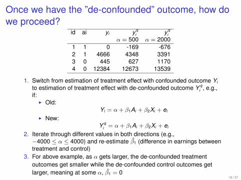
id ai yi yqi yq

iα = 500 α = 2000

1 1 0 -169 -6762 1 4666 4348 33913 0 445 627 11704 0 12384 12673 13539

1. Switch from estimation of treatment effect with confounded outcome Yi

to estimation of treatment effect with de-confounded outcome Y qi , e.g.,

if:I Old:

Yi = α + β1Ai + β2Xi + ei

I New:Y q

i = α + β1Ai + β2Xi + ei

2. Iterate through different values in both directions (e.g.,−4000 ≤ α ≤ 4000) and re-estimate β̂1 (difference in earnings betweentreatment and control)

3. For above example, as α gets larger, the de-confounded treatmentoutcomes get smaller while the de-confounded control outcomes getlarger, meaning at some α, β̂1 = 0

18 / 37

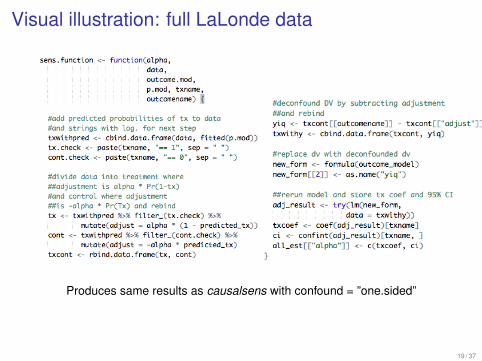
Visual illustration: full LaLonde data

Produces same results as causalsens with confound = ”one.sided”

19 / 37

Visual illustration: full LaLonde data

−4000

−3000

−2000

−1000

0

1000

2000

3000

4000

5000

6000

7000

−4000 −3000 −2000 −1000 0 1000 2000 3000 4000Amount of confounding (alpha)

Effe

ct o

f job

trai

ning

(AT

T)

−4000

−3000

−2000

−1000

0

1000

2000

3000

4000

5000

6000

7000

−4000 −3000 −2000 −1000 0 1000 2000 3000 4000Amount of confounding (alpha)

Effe

ct o

f job

trai

ning

(AT

E)

Figure: ATT on left corresponds to Figure 1 in paper; ATE is on right. Differ-ence stems from ATE: adjust both treatment and control yi versus ATT: adjustonly control yi with −αPr(Ai = 1|Xi )

20 / 37

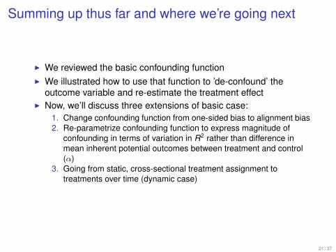
Summing up thus far and where we’re going next

I We reviewed the basic confounding functionI We illustrated how to use that function to ’de-confound’ the

outcome variable and re-estimate the treatment effectI Now, we’ll discuss three extensions of basic case:

1. Change confounding function from one-sided bias to alignment bias2. Re-parametrize confounding function to express magnitude of

confounding in terms of variation in R2 rather than difference inmean inherent potential outcomes between treatment and control(α)

3. Going from static, cross-sectional treatment assignment totreatments over time (dynamic case)

21 / 37

Extension one: change confounding function

I In previous example, checked how results change due toone-sided bias (q(1, x) = α; q(0, x) = −α), which captures thesituation where we expect those who select into treatment tohave inherently higher or lower values of outcome than thosewho select into control

I Lalonde example: those who opt for job training have inherentlyhigher or lower potential earnings than those who do not opt intotreatment

I Different confounding model: alignment bias(q(1, x) = q(0, x) = α) captures the situation where we expectthose who select into treatment to have larger treatment effectsthan those who select into control

I Lalonde example: those who opt for job training have unobservedcharacteristics that help them benefit more from job training than ifthose who did not opt for job training were subject to the treatment

22 / 37

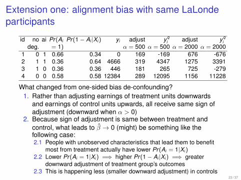
Extension one: alignment bias with same LaLondeparticipants

id no ai Pr(Ai Pr(1− Ai |Xi ) yi adjust yqi adjust yq

ideg. = 1) α = 500 α = 500 α = 2000 α = 2000

1 0 1 0.66 0.34 0 169 -169 676 -6762 1 1 0.36 0.64 4666 319 4347 1275 33913 1 0 0.36 0.36 446 181 265 725 -2794 0 0 0.58 0.58 12384 289 12095 1156 11228

What changed from one-sided bias de-confounding?1. Rather than adjusting earnings of treatment units downwards

and earnings of control units upwards, all receive same sign ofadjustment (downward when α > 0)

2. Because sign of adjustment is same between treatment andcontrol, what leads to β̂ → 0 (might) be something like thefollowing case:2.1 People with unobserved characteristics that lead them to benefit

most from treatment actually have lower Pr(Ai = 1|Xi )2.2 Lower Pr(Ai = 1|Xi ) =⇒ higher Pr(1− Ai |Xi ) =⇒ greater

downward adjustment of treatment group’s outcomes2.3 This is happening less (smaller downward adjustment) in controls

23 / 37

ATT: alignment bias (left) versus one-sided bias (right)with LaLonde data

−4000

−3000

−2000

−1000

0

1000

2000

3000

4000

5000

6000

7000

−4000 −3000 −2000 −1000 0 1000 2000 3000 4000Amount of confounding (alpha)

Effe

ct o

f job

trai

ning

(AT

E−

alig

nmen

t bia

s)

−4000

−3000

−2000

−1000

0

1000

2000

3000

4000

5000

6000

7000

−4000 −3000 −2000 −1000 0 1000 2000 3000 4000Amount of confounding (alpha)

Effe

ct o

f job

trai

ning

(AT

E−

one

−si

ded

bias

)

24 / 37

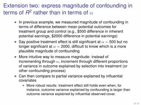
Extension two: express magnitude of confounding interms of R2 rather than in terms of α

I In previous example, we measured magnitude of confounding interms of difference between mean potential outcomes fortreatment group and control (e.g., $500 difference in inherentpotential earnings, $2000 difference in potential earnings)

I Say positive treatment effect is still significant at α = 500 but nolonger significant at α = 2000, difficult to know which is a moreplausible magnitude of confounding

I More intuitive way to measure magnitude: instead ofincrementing through α, increment through different proportionsof variance in outcome explained by selection into treatment (orother confounding process)

I Can then compare to partial variance explained by influentialcovariates

I More robust results: treatment effect still holds even when, forinstance, outcome variance explained by confounding is larger thanoutcome variance explained by influential observed covar.

25 / 37

Extension two: mechanics1. Start with proportion of potential outcome variance explained by

observed covariates X and treatment status A:

R2q(Xi ,Ai ) = 1− var [Yi (0)|Xi ,Ai ,q]

var [Yi (0)]

2. Then, find the proportion of potential outcome variance explainedby observed covariates X :

R2q(Xi ) = 1− var [Yi (0)|Xi ,q]

var [Yi (0)]

3. We can express the proportion of unexplained variance in thepotential outcomes due to selection into treatment by taking thevariance explained by X and selection into treatment andsubtracting out the variance explained by X (R2

q(Xi ,Ai )− R2q(Xi ))

and rearranging to get:

R2q(Ai ) = 1− var [Yi (0)|Xi ,Ai ,q]

var [Yi (0)|Xi ,q]

26 / 37

Extension two: mechanics

I Another way to express (3) from previous slide is as:

R2q(Ai ) = 1− var [Yi (0)|Xi ,Ai , q]

var [Yi (0)|Xi , q]= 1− unrestricted model

restricted model= 1− var(ei )

var(e′i )

I Then, assuming q is expressed as one-sided bias:1. Start with:

R2q(Ai ) = 1− var(ei )

var(e′i )

2. Simplify and plug in e′i = αAi + ei to numerator:

R2q(Ai ) =

var(αAi + ei )− var(ei )

var(e′i )

3. Use var(aX ) = a2var(x) and var(x + y) = var(x) + var(y) tofurther simplify:

R2q(Ai ) =

α2var(Ai ) + var(ei )− var(ei )

var(e′i )=α2var(Ai )

var(e′i )

27 / 37

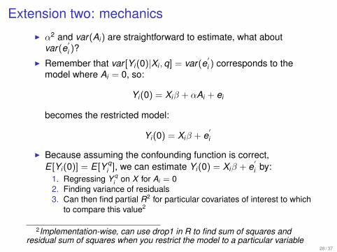
Extension two: mechanics

I α2 and var(Ai ) are straightforward to estimate, what aboutvar(e

′

i )?I Remember that var [Yi (0)|Xi ,q] = var(e

′

i ) corresponds to themodel where Ai = 0, so:

Yi (0) = Xiβ + αAi + ei

becomes the restricted model:

Yi (0) = Xiβ + e′

i

I Because assuming the confounding function is correct,E [Yi (0)] = E [Y q

i ], we can estimate Yi (0) = Xiβ + e′

i by:1. Regressing Y q

i on X for Ai = 02. Finding variance of residuals3. Can then find partial R2 for particular covariates of interest to which

to compare this value2

2Implementation-wise, can use drop1 in R to find sum of squares andresidual sum of squares when you restrict the model to a particular variable

28 / 37

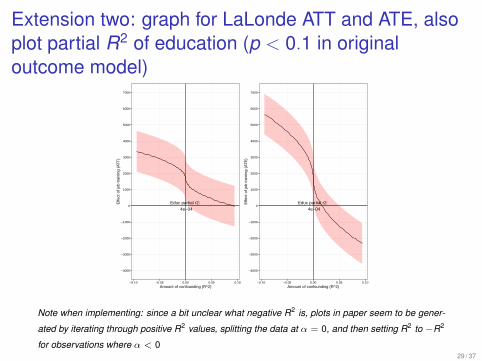
Extension two: graph for LaLonde ATT and ATE, alsoplot partial R2 of education (p < 0.1 in originaloutcome model)

Educ partial r2:

4e−04

−4000

−3000

−2000

−1000

0

1000

2000

3000

4000

5000

6000

7000

−0.10 −0.05 0.00 0.05 0.10Amount of confounding (R^2)

Effe

ct o

f job

trai

ning

(AT

T)

Educ partial r2:

4e−04

−4000

−3000

−2000

−1000

0

1000

2000

3000

4000

5000

6000

7000

−0.10 −0.05 0.00 0.05 0.10Amount of confounding (R^2)

Effe

ct o

f job

trai

ning

(AT

E)

Note when implementing: since a bit unclear what negative R2 is, plots in paper seem to be gener-

ated by iterating through positive R2 values, splitting the data at α = 0, and then setting R2 to −R2

for observations where α < 029 / 37

Extension three: time-varying treatments andconfounding

Motivation:I Previous examples were treatments and covariates observed at

one point in time (e..g, one-shot job training)I Blackwell (2012) argues that at least some treatments social

scientists care about are composed of action histories, a specificsequence of treatments

I Example: decisions to run negative (Ai = 1) versus positivecampaign ads at different weeks leading up to an election

campaign Week 1 Week 2 Week 3 Week 4 Vote share1 Neg Neg Neg Pos 67%2 Pos Neg Pos Neg 30%3 Neg Neg Neg Neg 47%

I These cases have more thorny dilemma than the single-shottreatment confounder issue: time-varying confounders, which areboth affected by past treatments and influence choice oftreatment at time t (e.g., poll results from week 2 beinginfluenced by neg v. pos ad at week 1 and influencing probabilityof negative campaign at week 3)

30 / 37

Extension three: from ignorability to sequentialignorability

I Single-shot treatment case: rests on ignorability assumption andsensitivity analysis probes how results change with violations

I Dynamic treatment case: rests on sequential ignorabilityassumption; likewise, sensitivity analysis probes consequencesof violations (notation: history of a variable up to time t):

Yi (a)⊥Ait |X it ,Ait−1

I Confounding function in dynamic treatment case:

qt (a, x t ) = E [Y (a)|At = at ,X t = x t ,At−1 = at−1]

− E [Y (a)|At = 1− at ,X t = x t ,At−1 = at−1]

I How do we use that confounding function to adjust the outcomevariable?

Yαi = Yi −

T∑t=0

qt (Ait ,X it ;α)Pr(At = 1− Ait |Ait−1,X it )

31 / 37

Extension three mechanics: de-confounding outcomein dynamic case

1. First, model the probability of treatment in week t conditionalupon X it and Ait . E.g., letting Ait = 1 = negative campaign ad forcampaign i in week t if t = 3:

Pr(Ai3 = 1) = α + β1negi1(1 = yes; 0 = no) + β2negi2(1 = yes; 0 = no)

+ β3donationi1 + β4donationi2 + β4donationi3 + ei

2. Using fitted values from 1, assign each i at each t the following,which is 1 minus the probability of reaching this treatmenthistory: Pr(At = 1− Ait |Ait−1,X it ) and multiply by appropriate α(e.g, alignment versus one-sided bias)

3. For each i , sum the results of (2) across t and subtract from Yi tocreate Yα

i , which is then used in whatever estimation procedurefor treatment effect is chosen (e.g., marginal structural model)

32 / 37

Extension three: Blackwell’s results for negativecampaign case, discuss interpretation

33 / 37

Briefly: alternative approaches (Morgan and Winship)I Blackwell and Rosenbaum correspond to Section 12.3

(”Sensitivity Analysis for Provisional Causal Effects Estimate”)I Authors outline a different approach in Section 12.2 where rather

than investigating the sensitivity of a treatment’s point estimate toviolations of strong assumptions like ignorability, we placebounds on the causal effect of treatment by adding weakassumptions

I Bounding, with work by Manski and more recently Keele, outlinesdifferent strategies for bounding causal quantities of interest likethe Average Treatment Effect (ATE):

1. No-assumptions bounds: if outcome variable is constrained to liebetween 0 and 1, the initial bounds on the treatment effectATE = [−1, 1] (width = 2) can be shrunk to bounds where width = 1by assuming different combinations of quantities for unobservedoutcomes (e.g., E [Y = 1|A = 0] = 1 and E [Y = 0|A = 1] = 0, andvice versa)

2. Weak assumptions bounds: can narrow width of interval (mosthelpfully so that the bounds exclude 0) through various weakassumptions: e.g., monotone treatment response, monotonetreatment selection

34 / 37

Recap/some questions1. What we reviewed: why sensitivity analysis? Rosenbaum bounds

approach; Blackwell approach: simple case and three extensions(different confounding function; re-parametrization of magnitude ofconfounding; dynamic treatment)...some questions:

2. One advantage of Blackwell is flexibility to create a confounding functionspecific to a theoretical story. Yet most examples drew on one-sidedbias (with some alignment bias). Other ideas for confounding functionsbeyond these?

3. Blackwell argues that one limitation of his approach is that at its core, itrelies on a ”selection on the observables” assumption so it is”incompatible with certain other approaches to causal inference such asinstrumental variables”(p. 181). Yet Morgan and Winship argue that”selection-bias models are most effectively estimated” when we includeinstrumental variables in Z . For the step in Blackwell’s approach wherewe estimate each unit’s probability of treatment, can we use aninstrumental variable as part of this estimation?

4. Dynamic treatment approach (action history) was developed inbiostatistics where we care about quantities like cumulative treatmenthistory. We have Blackwell’s negative ad example; what other socialscience questions would benefit from a treatment-history type approach(with accompanying sensitivity checks)?

35 / 37

Appendix

36 / 37

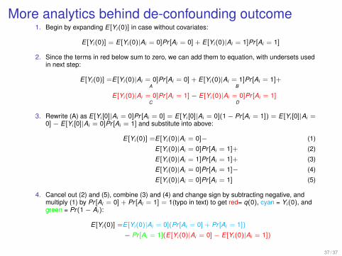
More analytics behind de-confounding outcome1. Begin by expanding E [Yi (0)] in case without covariates:

E [Yi (0)] = E [Yi (0)|Ai = 0]Pr [Ai = 0] + E [Yi (0)|Ai = 1]Pr [Ai = 1]

2. Since the terms in red below sum to zero, we can add them to equation, with undersets usedin next step:

E [Yi (0)] =E [Yi (0)|Ai = 0]Pr [Ai = 0]A

+ E [Yi (0)|Ai = 1]Pr [Ai = 1]B

+

E [Yi (0)|Ai = 0]Pr [Ai = 1]C

− E [Yi (0)|Ai = 0]Pr [Ai = 1]D

3. Rewrite (A) as E [Yi [0]|Ai = 0]Pr [Ai = 0] = E [Yi [0]|Ai = 0](1− Pr [Ai = 1]) = E [Yi [0]|Ai =0]− E [Yi [0]|Ai = 0]Pr [Ai = 1] and substitute into above:

E [Yi (0)] =E [Yi (0)|Ai = 0]− (1)

E [Yi (0)|Ai = 0]Pr [Ai = 1]+ (2)

E [Yi (0)|Ai = 1]Pr [Ai = 1]+ (3)

E [Yi (0)|Ai = 0]Pr [Ai = 1]− (4)

E [Yi (0)|Ai = 0]Pr [Ai = 1] (5)

4. Cancel out (2) and (5), combine (3) and (4) and change sign by subtracting negative, andmultiply (1) by Pr [Ai = 0] + Pr [Ai = 1] = 1(typo in text) to get red= q(0), cyan = Yi (0), andgreen = Pr(1− Ai ):

E [Yi (0)] =E [Yi (0)|Ai = 0](Pr [Ai = 0] + Pr [Ai = 1])

− Pr [Ai = 1](E [Yi (0)|Ai = 0]− E [Yi (0)|Ai = 1])

37 / 37