Global Development Policy Center Boston University 53 Bay State Road Boston, MA 02155 bu.edu/gdp An ECI Teaching Module on Social and Environmental Issues in Economics By Brian Roach, Pratistha Joshi Rajkarnikar, Neva Goodwin, and Jonathan M. Harris Social and Economic Inequality
Transcript
Global Development Policy CenterBoston University53 Bay State RoadBoston, MA 02155
bu.edu/gdp
An ECI Teaching Module on Social and Environmental Issues in Economics
By Brian Roach, Pratistha Joshi Rajkarnikar, Neva Goodwin, and Jonathan M. Harris
Social and Economic Inequality
Economics in Context Initiative, Global Development Policy Center, Boston University, 2020.
Permission is hereby granted for instructors to copy this module for instructional purposes.
Suggested citation: Roach, Brian, Pratistha Joshi Rajkarnikar, Neva Goodwin, and Jonathan
Harris. (2020) “Social and Economic Inequality.” An ECI Teaching Module on Social and
Economic Issues, Economics in Context Initiative, Global Development Policy Center, Boston
University, 2020.
Students may also download the module directly from:
As the United States economy began recovering from the Great Recession of 2007-2009, economic
data indicated that the vast majority of all income growth was going to the richest Americans.
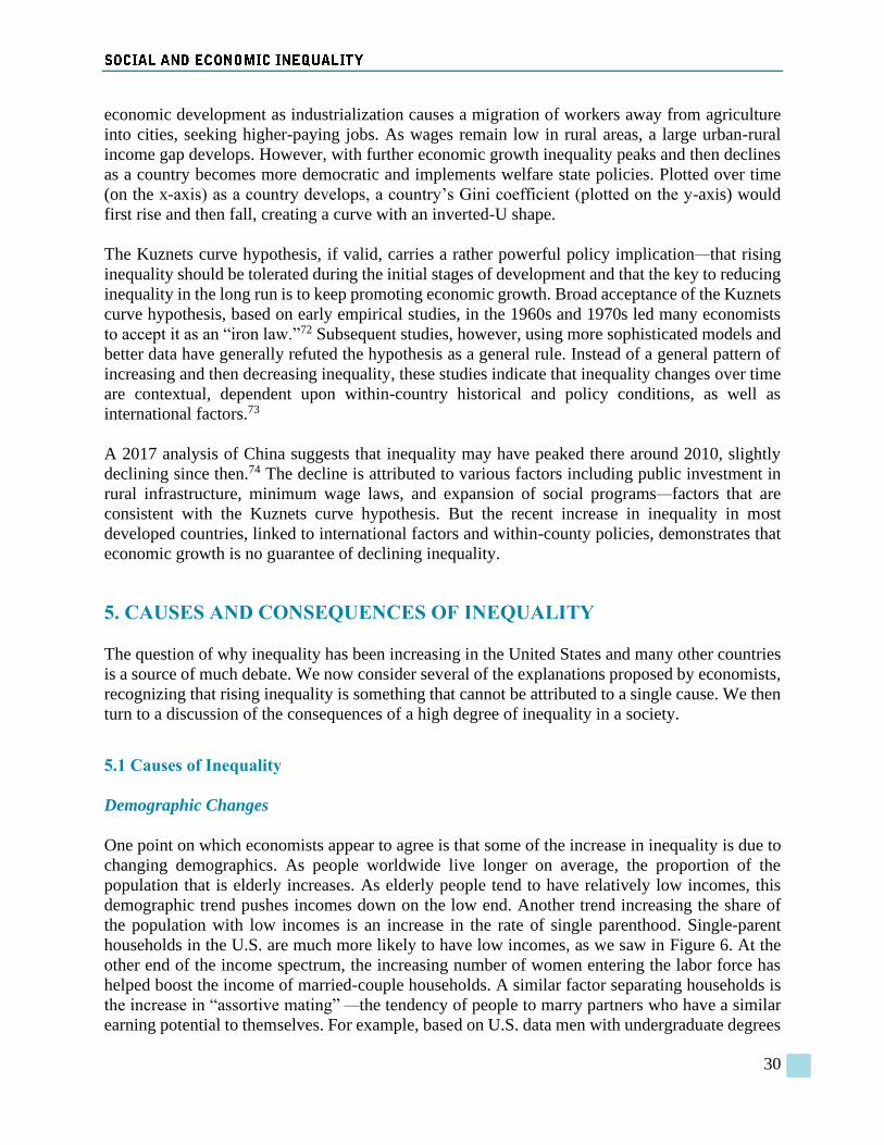
From 2009-2012, over 90% of new income accrued to just the top 1% of income earners. As the
economy recovered further, new income distribution was less lopsided, but still uneven. The top
1% captured over half of all income growth in the U.S. over the period 2009-2015.1
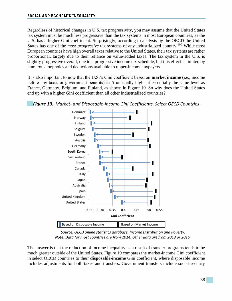
The trend toward higher economic inequality is not limited to the United States. Over the last few
decades, inequality has been increasing in most industrialized nations, as well as most of Asia,
including China and India. And while inequality has generally been decreasing in Latin American
and Sub-Saharan African countries, these regions still have the highest overall levels of inequality.2
Analysis of inequality, like most economic issues, involves both positive and normative questions.
Positive analysis can help us measure inequality, determine whether it is increasing or decreasing,
and explore the causes and consequences of inequality. But whether current levels of inequality
are acceptable, and what policies, if any, should be implemented to counter inequality are
normative questions. While our discussion of inequality here focuses mainly on positive analysis,
we will also consider the ethical and policy debates that are often driven by strongly-held values.
2. DEFINING AND MEASURING INEQUALITY
We begin our discussion of inequality by describing some objective measures of inequality, which
allow us to draw comparisons over time and across societies. We will first consider what we are
measuring, and then how we measure it.
2.1 Inequality of What?
When the subject of inequality is raised, most people think of income or wealth inequality. These
are indeed central to any economic analysis of the topic. But it is also important to recognize that
inequality is a broader concept that extends beyond the realm of money.
Let us consider a few examples. Vast inequality exists in the quality of health care across the world.
Preventable or treatable diseases in numerous tropical countries (such as malaria, measles, and
tuberculosis) cause average life expectancy to be significantly shorter than in the United States or
in other rich countries. There is also significant health inequality within many countries. According
to a 2017 analysis, average life expectancy in the United States is 10-15 years longer for the
wealthiest Americans than for the poorest.3 Early reports on the global pandemic of COVID-19
also expose inequities in the U.S. health system, as the impacts fall disproportionately on low
income households and communities of color (See Box 1).
There is also a considerable imbalance in education, both nationally and internationally. Children
in Australia can expect to receive, on average, about 20 years of schooling—the most years of any
country. Meanwhile, the average for children in the Sub-Saharan countries of Niger, Chad, and the
Central African Republic is less than eight years of education.4 Inequalities arise not only due to
5
income differences, but also due to race and gender. In the United States, the difference in
academic achievement between white and black students has decreased significantly in recent
decades but still remains evident. However, the achievement gap between students from low- and
high-income families in the U.S. has dramatically increased.5 There are mixed results for gender-
based educational inequality. By 2016, 24 countries had fully closed the educational gap by gender,
while in 17 countries women still had less than 90% of the educational outcomes that men have.6
BOX 1: COVID-19 AND ECONOMIC INEQUALITY
Prior to the emergence of COVID-19, income inequality in the United States was already at or
near record levels (see Figure 4). As the pandemic persists, it is becoming increasingly clear
that it will drive inequality even higher. A survey conducted in April 2020 found that 84% of
economic experts believed that the COVID-19 crisis will lead to a disproportionate economic
impact on low-income workers.7 Federal Reserve Chairman Jerome Powell said in May 2020
that:
The pandemic is falling on those least able to bear its burdens. It is a great increaser of
inequality. It is low-paid workers who are bearing the brunt of this and women to an
extraordinary degree.8
There are at least three related reasons why COVID-19 is increasing economic inequality in the
U.S.:
1. According to the U.S. Bureau of Labor Statistics, workers with higher incomes are more
likely to be able to work from home.9 In 2018 over 61% of workers with earnings in the
top 25% were classified as being able to work from home. Meanwhile, only 15% of
workers in the bottom half of earnings were classified as being able to work from home.
Thus higher-income workers have been more likely to make the transition to working at
home, or were already working from home, and have avoided a disruption to their
employment from the pandemic.
2. Sectors of the economy disproportionately affected by COVID-19 have lower average
wages. The BLS identifies industries such as restaurants, transportation, entertainment,
and retail as those that have been more exposed to negative economic impacts from the
pandemic.10 These “highly exposed” sectors have average full-time earnings of
$17/hour. Meanwhile, those sectors classified as “not highly exposed” to impacts from
the pandemic have average earnings of $23/hour. On average, the higher a family’s
income prior to the pandemic, the more likely their earnings came from employment in
a sector considered not highly exposed.
3. Less educated, and thus lower income, workers have been more likely to lose their jobs
as a result of the pandemic. According to the BLS, in May 2020 the unemployment rate
was 15.0% for high school graduates but 7.2% for those with a college degree.11
Comparing May 2020 to May 2019, the unemployment rate rose by nearly 12 percentage
points for high school graduates, but only 5 percentage points for college graduates.
6
The income losses by lower-income groups are particularly damaging given their lack of wealth.
Wealth inequality in the U.S. is significantly higher than income inequality (see Figure 7).
Households with little to no wealth have nothing to fall back on if their income is disrupted from
the pandemic. Further, initial statistics suggest that people in low-income and minority
households have been more likely to contract, and die from, COVID-19.12
Of course the increase in economic inequality as a result of COVID-19 is evident not just in the
U.S., but across the world. Previous health crises, such as SARS in 2003 and MERS in 2012,
caused a rise in affected countries’ Gini coefficient that persisted for years.13 The World Bank
has estimated that the pandemic will push about 50 million people globally into extreme
poverty.14 Sub-Saharan Africa, with limited health resources, is likely to be the hardest hit
region with an increase in extreme poverty of 23 million people.
The disproportionate impacts of COVID-19 can be mitigated through targeted public policies.
According to researchers from the International Monetary Fund,
Access to sick leave, unemployment benefits, and health benefits is useful for all in
dealing with the effects of the pandemic but particularly so for poorer segments of
society who lack a savings cushion and are thus living hand-to-mouth. … Expanding
social assistance systems, introducing new transfers, boosting public work programs
… and progressive tax measures—all are likely to be part of the policy mix to take
the edge off the devastating distributional consequences from the pandemic.15
Related to both health and education is what Nobel laureate Amartya Sen has famously referred to
as “capabilities.” By his reckoning, money is only one dimension—albeit an important one—of an
individual’s “capability” to function in his or her economic environment. To Sen, what matters
most is that people possess the necessary tools—including money, health, education, friends, and
social connections—to provide them with realistic economic choices. As Sen has pointed out, there
is considerable inequality of capabilities in the world, not just in the poor countries.
Inequality is also manifested in certain environmental outcomes. Proponents of “environmental
justice,” point out that polluting industries and toxic waste disposal sites in the United States tend
to be located disproportionately near poor and minority communities. This effect is even more
pronounced in some developing countries. Oil and gas development in Nigeria by international
corporations has resulted in thousands of oil spills that have impoverished local residents due to
reduced agricultural production, lower fish harvests, and polluted drinking water.16 In many
developed countries, there are stronger regulations on industrial pollution, but major impacts from
oil and chemical spills and other emissions still occur, often affecting lower-income communities.
One also sees considerable inequality when confronting the issue of climate change. Numerous
studies find that climate change will hit poor countries the hardest, exacerbating global inequality.
Warmer temperatures and changing precipitation patterns in Africa and other developing regions
could reduce the growing season and lower yields, leading to a 20% global increase in the number
of people at risk of hunger by 2050.17 According to a 2015 analysis in the journal Nature, by the
7
end of the 21st century climate change will have a significantly higher proportionate impact on
incomes in the world’s poorest.18 In addition to these specific effects, a critical fact about climate
change, as well as other environmental damage, is that the rich can generally protect themselves
much better than the poor can.
2.2 Measuring Inequality
While recognizing these various types of inequality, for the purposes of economic analysis we will
focus primarily on inequality of income and wealth. The two most common metrics used to
measure income inequality are:
1. Measure the income share (percent of all income) held by various groups ordered by
income from poorest to richest, such as the bottom 20%, the middle 20%, the top 1%, etc.
2. Measure the overall distribution of income in a society, using mathematical and graphical
techniques.
Income Distribution Data
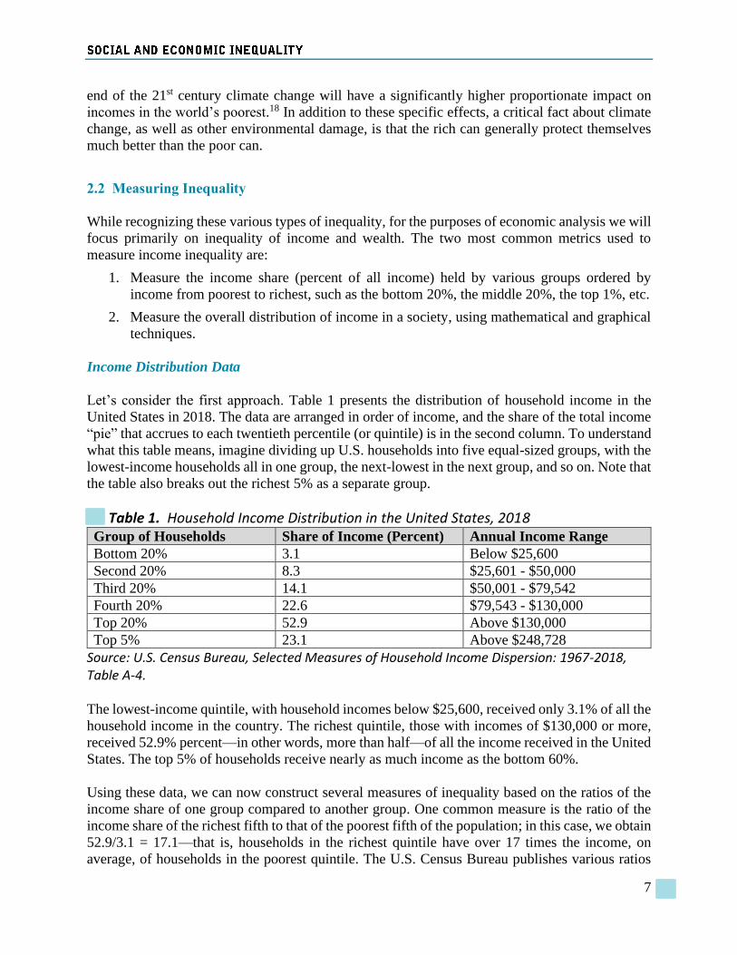
Let’s consider the first approach. Table 1 presents the distribution of household income in the
United States in 2018. The data are arranged in order of income, and the share of the total income
“pie” that accrues to each twentieth percentile (or quintile) is in the second column. To understand
what this table means, imagine dividing up U.S. households into five equal-sized groups, with the
lowest-income households all in one group, the next-lowest in the next group, and so on. Note that
the table also breaks out the richest 5% as a separate group.
Table 1. Household Income Distribution in the United States, 2018 Group of Households Share of Income (Percent) Annual Income Range
Bottom 20% 3.1 Below $25,600
Second 20% 8.3 $25,601 - $50,000
Third 20% 14.1 $50,001 - $79,542
Fourth 20% 22.6 $79,543 - $130,000
Top 20% 52.9 Above $130,000
Top 5% 23.1 Above $248,728
Source: U.S. Census Bureau, Selected Measures of Household Income Dispersion: 1967-2018, Table A-4.
The lowest-income quintile, with household incomes below $25,600, received only 3.1% of all the
household income in the country. The richest quintile, those with incomes of $130,000 or more,
received 52.9% percent—in other words, more than half—of all the income received in the United
States. The top 5% of households receive nearly as much income as the bottom 60%.
Using these data, we can now construct several measures of inequality based on the ratios of the
income share of one group compared to another group. One common measure is the ratio of the
income share of the richest fifth to that of the poorest fifth of the population; in this case, we obtain
52.9/3.1 = 17.1—that is, households in the richest quintile have over 17 times the income, on
average, of households in the poorest quintile. The U.S. Census Bureau publishes various ratios
8
based on the incomes at different percentiles of the distribution, such as the 90th/10th ratio, the
95th/20th ratio, and the 80th/50th ratio. We can see how these ratios have changed over time to track
changes in inequality. For example, the ratio of income share between the richest fifth to that of
the poorest fifth in the United States has increased from only about 10 in 1980 to over 17 in 2018,
indicating an increase in the spread between the richest and poorest fifth of the population.
The Lorenz Curve and Gini Coefficients
A simple ratio of income shares between two groups is somewhat arbitrary, focusing on some parts
of the income distribution while ignoring others. A more comprehensive measure that reflects the
entire income distribution involves creating a graph of the income distribution, referred to as a
Lorenz curve—named after Max Lorenz, the statistician who first developed the technique. A
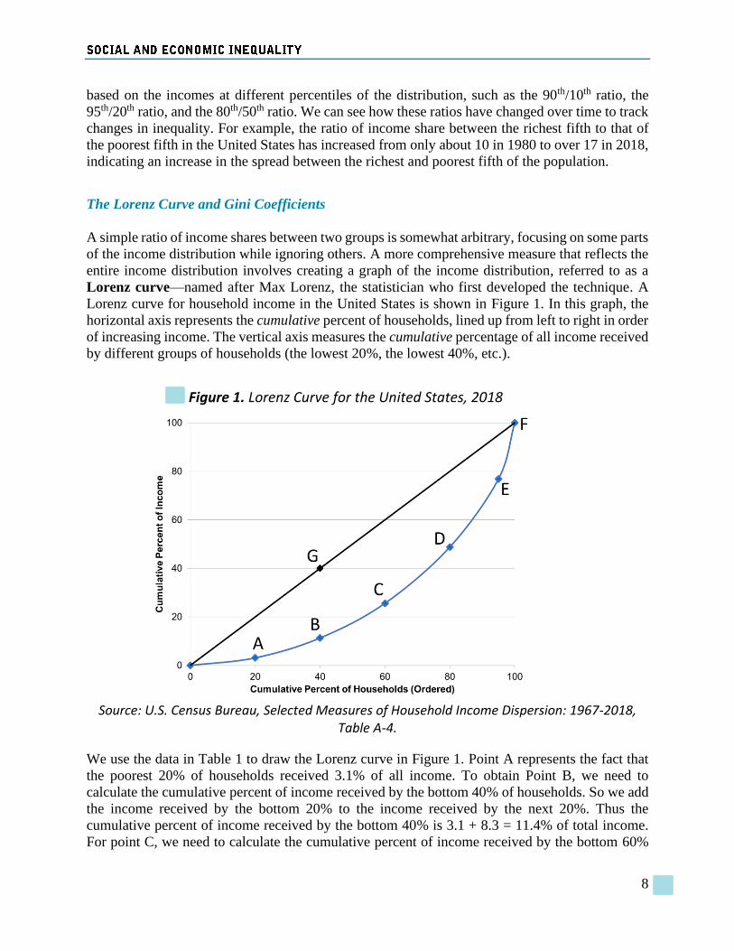
Lorenz curve for household income in the United States is shown in Figure 1. In this graph, the
horizontal axis represents the cumulative percent of households, lined up from left to right in order
of increasing income. The vertical axis measures the cumulative percentage of all income received
by different groups of households (the lowest 20%, the lowest 40%, etc.).
Figure 1. Lorenz Curve for the United States, 2018
Source: U.S. Census Bureau, Selected Measures of Household Income Dispersion: 1967-2018,
Table A-4.
We use the data in Table 1 to draw the Lorenz curve in Figure 1. Point A represents the fact that
the poorest 20% of households received 3.1% of all income. To obtain Point B, we need to
calculate the cumulative percent of income received by the bottom 40% of households. So we add
the income received by the bottom 20% to the income received by the next 20%. Thus the
cumulative percent of income received by the bottom 40% is 3.1 + 8.3 = 11.4% of total income.
For point C, we need to calculate the cumulative percent of income received by the bottom 60%
9
of households, which is 3.1 + 8.3 + 14.1 = 25.5% of total income. Similarly, point D shows that
the income share of the bottom 80% is 48% of all income. Finally, point E shows that the bottom
95% received 76.9% of all income (everyone except the top 5%). The Lorenz curve must start at
the origin, at the lower left corner of the graph (because 0% of households have 0% of the total
income) and must end at point F in the upper right corner (because 100% of households must have
100% of the total income).
The Lorenz curve provides information about the degree of income inequality in a country. Note
that the 45-degree line in Figure 1 represents a situation of absolute equality. If every household
had the same exact income, then, for example, the “bottom” 40% of households would receive
40% of all income. This is shown by point G in Figure 1. Imagine the other extreme—a situation
in which one household received all the income in a country. In this case, the Lorenz curve would
be a flat line along the horizontal axis at a value of zero until the very end, where it would suddenly
shoot up to 100 percent of income (at point F).
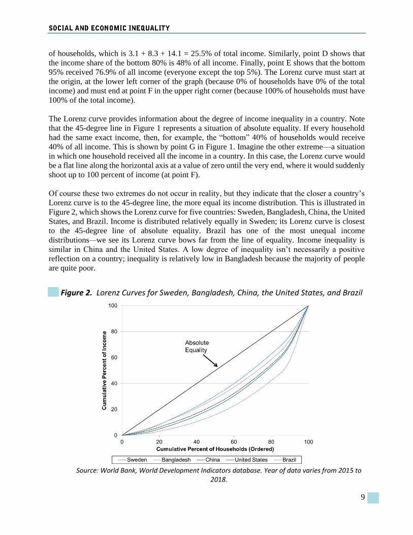
Of course these two extremes do not occur in reality, but they indicate that the closer a country’s
Lorenz curve is to the 45-degree line, the more equal its income distribution. This is illustrated in
Figure 2, which shows the Lorenz curve for five countries: Sweden, Bangladesh, China, the United
States, and Brazil. Income is distributed relatively equally in Sweden; its Lorenz curve is closest
to the 45-degree line of absolute equality. Brazil has one of the most unequal income
distributions—we see its Lorenz curve bows far from the line of equality. Income inequality is
similar in China and the United States. A low degree of inequality isn’t necessarily a positive
reflection on a country; inequality is relatively low in Bangladesh because the majority of people
are quite poor.
Figure 2. Lorenz Curves for Sweden, Bangladesh, China, the United States, and Brazil
Source: World Bank, World Development Indicators database. Year of data varies from 2015 to
2018.
10
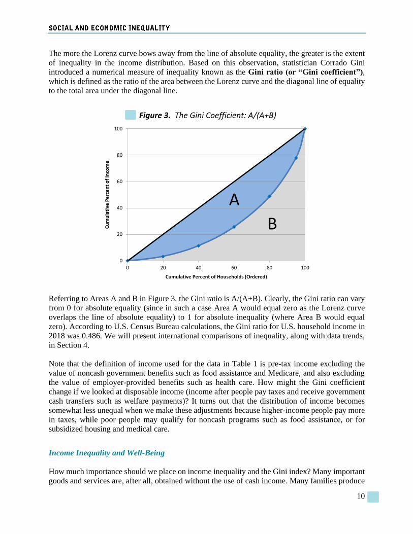
The more the Lorenz curve bows away from the line of absolute equality, the greater is the extent
of inequality in the income distribution. Based on this observation, statistician Corrado Gini
introduced a numerical measure of inequality known as the Gini ratio (or “Gini coefficient”),
which is defined as the ratio of the area between the Lorenz curve and the diagonal line of equality
to the total area under the diagonal line.
Figure 3. The Gini Coefficient: A/(A+B)
Referring to Areas A and B in Figure 3, the Gini ratio is A/(A+B). Clearly, the Gini ratio can vary
from 0 for absolute equality (since in such a case Area A would equal zero as the Lorenz curve
overlaps the line of absolute equality) to 1 for absolute inequality (where Area B would equal
zero). According to U.S. Census Bureau calculations, the Gini ratio for U.S. household income in
2018 was 0.486. We will present international comparisons of inequality, along with data trends,
in Section 4.
Note that the definition of income used for the data in Table 1 is pre-tax income excluding the
value of noncash government benefits such as food assistance and Medicare, and also excluding
the value of employer-provided benefits such as health care. How might the Gini coefficient
change if we looked at disposable income (income after people pay taxes and receive government
cash transfers such as welfare payments)? It turns out that the distribution of income becomes
somewhat less unequal when we make these adjustments because higher-income people pay more
in taxes, while poor people may qualify for noncash programs such as food assistance, or for
subsidized housing and medical care.
Income Inequality and Well-Being
How much importance should we place on income inequality and the Gini index? Many important
goods and services are, after all, obtained without the use of cash income. Many families produce
0
20
40
60
80
100
0 20 40 60 80 100
Cu
mu
lati
ve P
erc
en
t o
f In
com
e
Cumulative Percent of Households (Ordered)
B
A
11
at least some services (such as child care and cooking) for themselves. In addition, many of the
things that we enjoy—such as pleasant parks, safe roads, or clean air—add to our well-being
without requiring payments (although some of these things are financed through taxes). If we were
to look at the distribution of well-being rather than just the distribution of income, we would need
to take account of these other sources of important goods and services. Some of these goods may
contribute to lessening inequality—for example, everyone, rich or poor, can enjoy a public park
or use a public library. Evidence suggests, however, that at least in some cases the distribution of
such non-purchased goods may accentuate, rather than lessen, inequality. For example, as noted
earlier, proponents of “environmental justice” point out that polluting industries and toxic waste
disposal sites tend to be located disproportionately near poor and minority communities.
Another interesting issue is the relationship between income and leisure time. Data for the United
States indicate that higher education, and thus higher income, is associated with less leisure time.
But this does not mean that poor people simply enjoy lives of greater leisure and well-being.
Instead, unemployment rates are much higher for people with less education, suggesting that some
leisure time is involuntary. Meanwhile, job satisfaction increases with education, which also
contributes to well-being.19 As we’ve seen before, well-being is multi-dimensional and we should
be wary about drawing conclusions about well-being based on any single variable.
3. INEQUALITY TRENDS IN THE UNITED STATES
We can now use inequality data to track how inequality has changed over time. In this section, we
focus on economic inequality in the United States. We will explore trends in income inequality,
wealth inequality, and economic mobility, and provide some additional perspectives on
inequalities in labor market outcomes based on race, gender, age, and education. International data
on income and wealth inequality are presented in Section 4.
3.1 Income Inequality
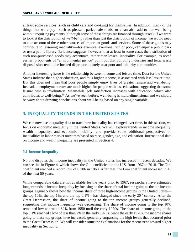
No one disputes that income inequality in the United States has increased in recent decades. We
can see this in Figure 4, which shows the Gini coefficient in the U.S. from 1967 to 2018. The Gini
coefficient reached a record low of 0.386 in 1968. After that, the Gini coefficient increased in 40
of the next 50 years.
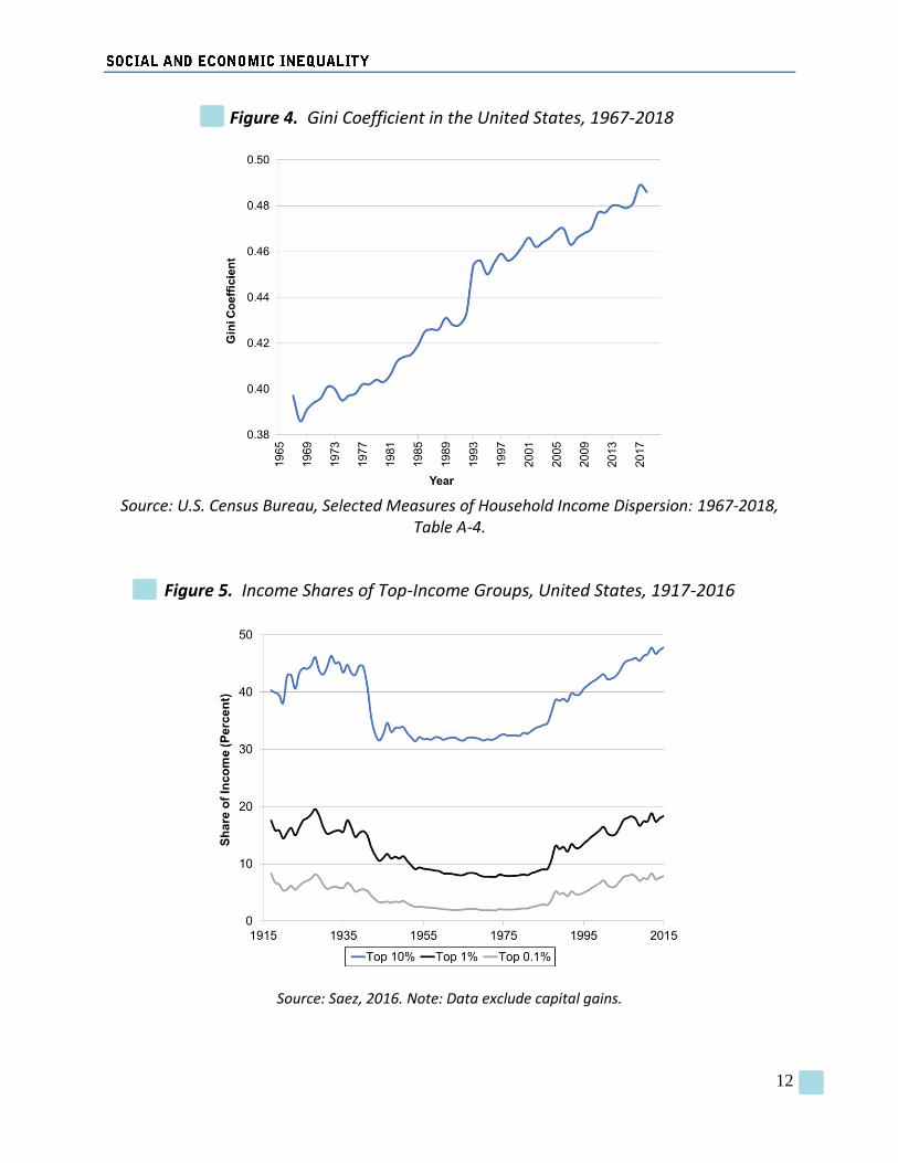
While comparable data are not available for the years prior to 1967, researchers have estimated
longer trends in income inequality by focusing on the share of total income going to the top income
groups. Figure 5 shows how the income share of three high-income groups in the United States—
the top 10%, the top 1%, and the top 0.1%—has changed since the early 20th century. After the
Great Depression, the share of income going to the top income groups generally declined,
suggesting that income inequality was decreasing. The share of income going to the top 10%
remained low at around 32% from 1950 until the early 1970s. The share of income going to the
top 0.1% reached a low of less than 2% in the early 1970s. Since the early 1970s, the income shares
going to these top groups have increased, generally surpassing the high levels that occurred prior
to the Great Depression. We will consider some the explanations for the recent trend toward higher
inequality in Section 5.
12
Figure 4. Gini Coefficient in the United States, 1967-2018
Source: U.S. Census Bureau, Selected Measures of Household Income Dispersion: 1967-2018,
Table A-4.
Figure 5. Income Shares of Top-Income Groups, United States, 1917-2016
Source: Saez, 2016. Note: Data exclude capital gains.
13
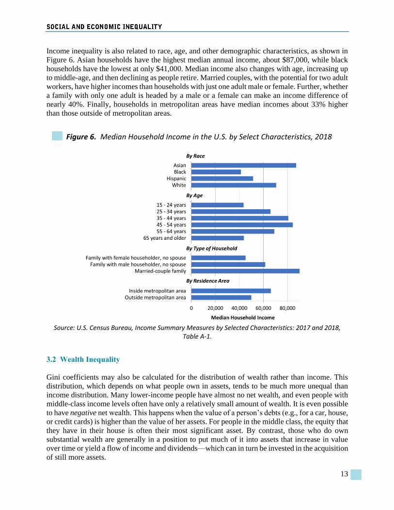
Income inequality is also related to race, age, and other demographic characteristics, as shown in
Figure 6. Asian households have the highest median annual income, about $87,000, while black
households have the lowest at only $41,000. Median income also changes with age, increasing up
to middle-age, and then declining as people retire. Married couples, with the potential for two adult
workers, have higher incomes than households with just one adult male or female. Further, whether
a family with only one adult is headed by a male or a female can make an income difference of
nearly 40%. Finally, households in metropolitan areas have median incomes about 33% higher
than those outside of metropolitan areas.
Figure 6. Median Household Income in the U.S. by Select Characteristics, 2018
Source: U.S. Census Bureau, Income Summary Measures by Selected Characteristics: 2017 and 2018,
Table A-1.
3.2 Wealth Inequality
Gini coefficients may also be calculated for the distribution of wealth rather than income. This
distribution, which depends on what people own in assets, tends to be much more unequal than
income distribution. Many lower-income people have almost no net wealth, and even people with
middle-class income levels often have only a relatively small amount of wealth. It is even possible
to have negative net wealth. This happens when the value of a person’s debts (e.g., for a car, house,
or credit cards) is higher than the value of her assets. For people in the middle class, the equity that
they have in their house is often their most significant asset. By contrast, those who do own
substantial wealth are generally in a position to put much of it into assets that increase in value
over time or yield a flow of income and dividends—which can in turn be invested in the acquisition
of still more assets.
14
The distribution of wealth is, however, less frequently and less systematically recorded than the
distribution of income—in part because wealth can be hard to measure. Much wealth is held in the
form of unrealized capital gains. A household realizes (turns into actual dollars) capital gains if it
sells an appreciated asset, such as shares in a company, land, or antiques, for more than the price
at which it purchased the asset. An asset can appreciate in value for a long time before it is actually
sold. No one, however, will know exactly how much such an asset has really gained or lost in
value until the owner actually does sell it, thus “realizing” the capital gain. Another reason that it
is harder to get information on wealth is that although governments normally require people to
report their annual income from wages and many investments for tax purposes, most governments
do not require regular and comprehensive reporting of asset holdings. Finally, wealth consists not
only of financial assets but also commodities, paintings, real estate, and the like. Such disparate
forms of wealth make it difficult to obtain reliable estimates of aggregate wealth statistics.
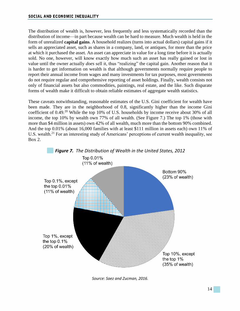
These caveats notwithstanding, reasonable estimates of the U.S. Gini coefficient for wealth have
been made. They are in the neighborhood of 0.8, significantly higher than the income Gini
coefficient of 0.49.20 While the top 10% of U.S. households by income receive about 30% of all
income, the top 10% by wealth own 77% of all wealth. (See Figure 7.) The top 1% (those with
more than $4 million in assets) own 42% of all wealth, much more than the bottom 90% combined.
And the top 0.01% (about 16,000 families with at least $111 million in assets each) own 11% of
U.S. wealth.21 For an interesting study of Americans’ perceptions of current wealth inequality, see
Box 2.
Figure 7. The Distribution of Wealth in the United States, 2012
Source: Saez and Zucman, 2016.
15
BOX 2: WEALTH INEQUALITY IN THE UNITED STATES
Political debates about inequality are often based on perceptions rather than facts. A 2011 study
surveyed people regarding their perceptions of wealth inequality in the U.S.22 Respondents were
asked to estimate what percentage of total wealth was actually owned by each wealth quintile.
They were also asked to construct their ideal distribution of wealth, again assigning a percentage
of total wealth to each quintile.
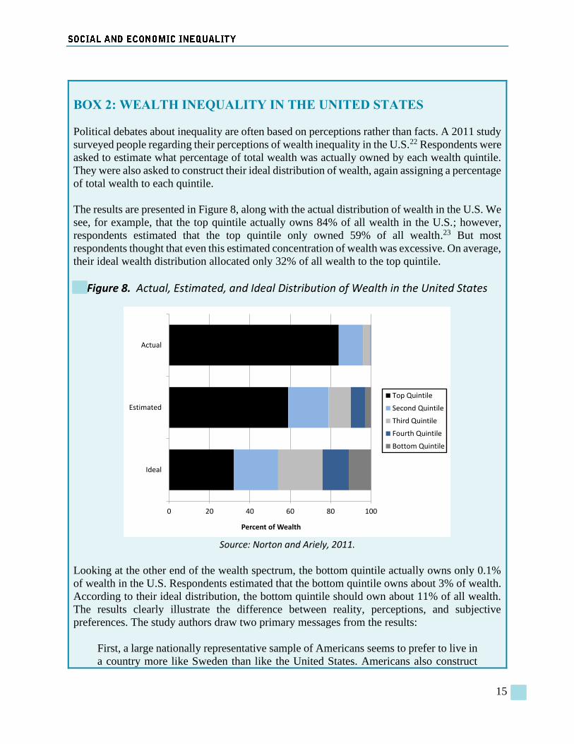
The results are presented in Figure 8, along with the actual distribution of wealth in the U.S. We
see, for example, that the top quintile actually owns 84% of all wealth in the U.S.; however,
respondents estimated that the top quintile only owned 59% of all wealth.23 But most
respondents thought that even this estimated concentration of wealth was excessive. On average,
their ideal wealth distribution allocated only 32% of all wealth to the top quintile.
Figure 8. Actual, Estimated, and Ideal Distribution of Wealth in the United States
Source: Norton and Ariely, 2011.
Looking at the other end of the wealth spectrum, the bottom quintile actually owns only 0.1%
of wealth in the U.S. Respondents estimated that the bottom quintile owns about 3% of wealth.
According to their ideal distribution, the bottom quintile should own about 11% of all wealth.
The results clearly illustrate the difference between reality, perceptions, and subjective
preferences. The study authors draw two primary messages from the results:
First, a large nationally representative sample of Americans seems to prefer to live in
a country more like Sweden than like the United States. Americans also construct
0 20 40 60 80 100
Ideal
Estimated
Actual
Percent of Wealth
Top Quintile
Second Quintile
Third Quintile
Fourth Quintile
Bottom Quintile
16
ideal distributions that are far more equal than they estimated the United States to
be—estimates which themselves were far more equal than the actual level of
inequality. Second, there was much more consensus than disagreement across groups
from different sides of the political spectrum about this desire for a more equal
distribution of wealth, suggesting that Americans may possess a commonly held
‘‘normative’’ standard for the distribution of wealth despite the many disagreements
about policies that affect that distribution, such as taxation and welfare.24
Just as income inequality has been increasing in recent decades, so has wealth inequality. A plot
of the wealth shares owned by the top groups in the U.S. over time looks much like the income
shares in Figure 5. The share of national wealth owned by the top 1% was over 50% prior to the
Great Depression, declined to less than 25% by the late 1970s, but then steadily increased to around
45% today.25
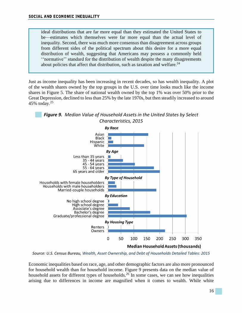
Figure 9. Median Value of Household Assets in the United States by Select Characteristics, 2015
Source: U.S. Census Bureau, Wealth, Asset Ownership, and Debt of Households Detailed Tables: 2015
Economic inequalities based on race, age, and other demographic factors are also more pronounced
for household wealth than for household income. Figure 9 presents data on the median value of
household assets for different types of households.26 In some cases, we can see how inequalities
arising due to differences in income are magnified when it comes to wealth. While white
17
households’ incomes are 71% higher than the incomes of black households, the assets of white
households are about 7 times higher than those of black households. Hispanic households also
have little in assets, only about $20,000. The median value of household assets tends to rise with
age. So while older households (aged 65 and older) have relatively low income as seen in Figure
6, they have comparatively high assets. While married couples have incomes about twice as high
as households with just one adult, their assets about 6 times larger. We also see that education has
a significant impact on household assets. For example, those with a college degree have over four
times as much household wealth as those with only a high school diploma. Finally, those owning
their own homes (including those still paying a mortgage) have 80 times the assets of renters. This
demonstrates the importance of real estate equity in building household wealth.
Contemplating such vast wealth inequality brings us back to the question of opportunity. Do those
with little or even negative wealth have the opportunity to achieve an adequate level of well-being?
In addition, great wealth often confers upon its owners both economic and political power. When
the ownership of wealth is highly uneven, the ability to direct the operations of businesses and to
influence government policy through campaign contributions and the like may become
concentrated in the hands of relatively few. They may then use this power to maintain or exacerbate
existing inequalities. We return to this point later in the module.
3.3 Economic Mobility
Our discussion above suggests that some inequality is to be expected in any society, given that
people’s incomes and assets tend to increase as they become older and more established in their
careers. At any point in time, we are likely to have younger people with relatively low incomes
and few assets, middle-aged people with higher incomes and more assets, and retirees who tend to
have relatively low incomes but relatively high assets. (See Figures 6 and 9.) Thus we have people
moving from lower income groups to higher income groups, and vice versa. This possibility for
people or households to change their economic status, for better or worse, is called economic
mobility. For a given level of economic inequality, we may be more tolerant if economic mobility
is higher because it implies that people have the opportunity to improve their economic condition.
A common way to measure economic mobility is to track the frequency with which individuals or
households move into different income groups, especially in relation to the group in which they
were raised. For example, a 2013 U.S. study looks at the income quintiles of people in their late
30s related to their “birth quintile”—the quintile where their parents were, at the same age.27 For
people raised in families from the bottom quintile, 44% are still in the bottom quintile as adults,
22% rise into the second quintile, and about 6% rise all the way to the top quintile. Meanwhile,
people raised in families from the top quintile are 47% likely to also be in the top quintile as adults,
with about 25% in the fourth quintile and 7% falling all the way to the bottom quintile. So while
some economic mobility exists, one’s background is clearly an important determinant of one’s
adult income. A 2015 study summarized the situation:
[C]hildren raised in low-income families will probably have very low incomes as
adults, while children raised in high-income families can anticipate very high
incomes as adults. The differences are extreme: The expected income of children
raised in well-off families (90th percentile) is about 200 percent larger than the
18
expected income of children raised in poor families (10th percentile) and about 75%
larger than that of children raised in middle-class families (50th percentile).28
A 2016 paper that studied economic mobility by looking at how one’s income changed throughout
a working career found that earnings mobility has decreased as inequality has increased since the
1980s.29 A particularly striking finding was a dramatic decline in upward mobility for those
starting their careers in the middle class, even for those with a college degree.
Another aspect of economic mobility is whether successive generations are, on average, better off
than their parents. With consistent economic growth, each generation can look forward to higher
average incomes. However, recent research suggests that this is no longer the case in the United
States. (See Box 3.)
BOX 3: THE FADING AMERICAN DREAM
One aspect of the “American Dream” is that each successive generation hopes it will be better
off than the previous generation. This continual increase in living standards is referred to as
“absolute income mobility.” While this was often taken for granted in the past, is this part of the
American Dream still alive?
According to a 2017 paper, the answer seems to be mostly “no.”30 Looking at data on children
born in the U.S. from 1940 to 1984, and their parents, the researchers were able to determine
the percentage of children that ended up earning more than their parents (after adjusting for
inflation). For children born in 1940, over 90% of them ended up earning more than their
parents. But for children born in the 1980s, this percentage had dropped to 50%.
Two explanations for the decline in absolute income mobility are proposed: lower GDP growth
rates and greater income inequality. Of these two explanations, the paper concludes that:
most of the decline in absolute mobility is driven by the more unequal distribution of
economic growth in recent decades, rather than by the slowdown in GDP growth
rates. In this sense, the rise in inequality and the decline in absolute mobility are
closely linked. Growth is an important driver of absolute mobility, but high levels of
absolute mobility require broad-based growth across the income distribution. With
the current distribution of income, higher GDP growth rates alone are insufficient to
restore absolute mobility to the levels experienced by children in the 1940s and
1950s. If one wants to revive the “American dream” of high rates of absolute
mobility, then one must have an interest in growth that is spread more broadly across
the income distribution.31
19
3.4 Inequality and Labor Market Outcomes
One aspect that is particularly important in understanding trends in inequality is the differences in
labor market outcomes for individuals from different demographic groups. In the United States, it
is generally true that opportunities to have good paid work, with good compensation, are greater
for men than for women; for younger people than for older ones; for the more educated than for
the less educated; and for white, native-born Americans than for immigrants or people of color.
We will now explore these realities by considering the role of labor market discrimination,
which exists when, among similarly qualified people, some are treated disadvantageously in
employment on the basis of race, sex, age, sexual preference, physical appearance, or disability.
Workers who belong to disfavored groups may be paid less for the same work, may be denied
promotions, or may simply be excluded from higher-paying and higher-status occupations.
Inequality based on Race and Ethnicity
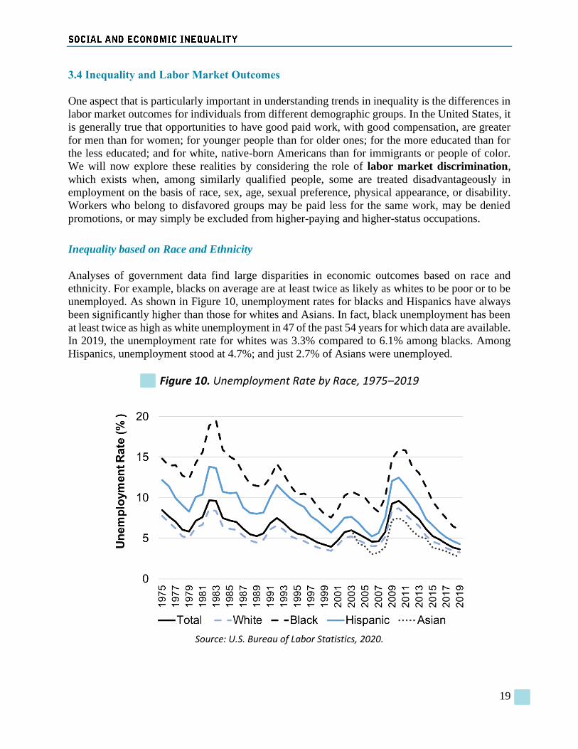
Analyses of government data find large disparities in economic outcomes based on race and
ethnicity. For example, blacks on average are at least twice as likely as whites to be poor or to be
unemployed. As shown in Figure 10, unemployment rates for blacks and Hispanics have always
been significantly higher than those for whites and Asians. In fact, black unemployment has been
at least twice as high as white unemployment in 47 of the past 54 years for which data are available.
In 2019, the unemployment rate for whites was 3.3% compared to 6.1% among blacks. Among
Hispanics, unemployment stood at 4.7%; and just 2.7% of Asians were unemployed.
Figure 10. Unemployment Rate by Race, 1975–2019
Source: U.S. Bureau of Labor Statistics, 2020.
20
The higher unemployment among minority groups, is at least partly due to discrimination in the
labor market. Researchers studying race-based discrimination have used experiments that explore,
for example, how employers respond to job applicants with “minority-sounding” names. A 2017
paper that reviewed the results of 28 such studies found that applicants with white names like
Emily and Greg receive, on average, 36% more callbacks than applicants with names like Lakisha
and Jamal, and 24% more callbacks than applicants that appear to be Latinos.32 The degree of
discrimination against black applicants has not declined since 1989, but has declined slightly
against Latinos.
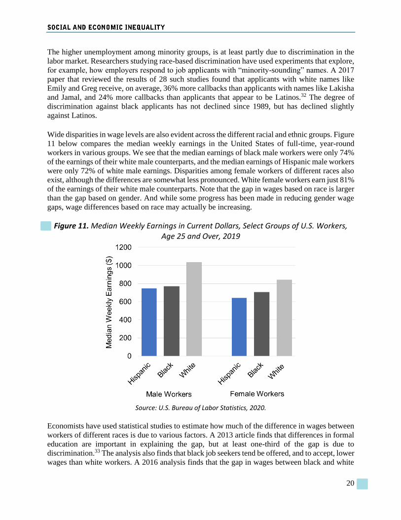
Wide disparities in wage levels are also evident across the different racial and ethnic groups. Figure
11 below compares the median weekly earnings in the United States of full-time, year-round
workers in various groups. We see that the median earnings of black male workers were only 74%
of the earnings of their white male counterparts, and the median earnings of Hispanic male workers
were only 72% of white male earnings. Disparities among female workers of different races also
exist, although the differences are somewhat less pronounced. White female workers earn just 81%
of the earnings of their white male counterparts. Note that the gap in wages based on race is larger
than the gap based on gender. And while some progress has been made in reducing gender wage
gaps, wage differences based on race may actually be increasing.
Figure 11. Median Weekly Earnings in Current Dollars, Select Groups of U.S. Workers, Age 25 and Over, 2019
Source: U.S. Bureau of Labor Statistics, 2020.
Economists have used statistical studies to estimate how much of the difference in wages between
workers of different races is due to various factors. A 2013 article finds that differences in formal
education are important in explaining the gap, but at least one-third of the gap is due to
discrimination.33 The analysis also finds that black job seekers tend be offered, and to accept, lower
wages than white workers. A 2016 analysis finds that the gap in wages between black and white
21
workers in the U.S. narrowed in the 1990s due to low unemployment and minimum wage
increases, but has increased since 2000 as black workers were more negatively impacted by the
Great Recession.34
Disadvantages in jobs and wages translate, of course, to disadvantages in income and wealth.
Although the poverty rate for blacks has come down significantly since the mid-1970s, as of 2014
blacks were still more than twice as likely as whites to be living in poverty (26% compared with
10%). Also, 2016 Census data shows that women in all racial and ethnic groups were more likely
than white, non-Hispanic men to be in poverty. Specifically, 21.4% of black women, 22.8% of
Native American women, 18.7% of Latino women and 10.7% of Asian women lived in poverty.
As a comparison, 9.7% of white women, and 7% of white men, were described as living in poverty.
Gender-Based Inequality
The gender wage gap—the difference in average wages between men and women—has declined
in the United States in recent decades.35 In 1980 women’s average wages were 64% of men’s
wages. By 2019 the gap had been reduced by about half, but women still earned only about 82%
of men’s wages.
Historically, the gender wage gap has resulted from a number of factors, including:
• Simple discrimination caused women to be passed over, in favor of men, for promotion.
• Women have often received less compensation than men in identical jobs.
• Young women sometimes deferred entrance to the labor force while they had young
children, or else worked shorter hours in the early part of their careers; hence they had less
seniority. When family members were ill, women were more likely to take time off work
to care for them, giving an impression of lower job attachment.
• Occupational segregation—the tendency of men and women to be found in different
kinds of jobs—is also important in explaining earnings differences by gender. For example,
in the United States, jobs like child-care worker, registered nurse, and preschool teacher
are held overwhelmingly by women. Meanwhile, men dominate in occupations such as
construction trades, metal working, truck driving, and engineering. Occupational
segregation could be a result of differences in preferences, or it could also reflect
discrimination. For example, existing stereotypes may lead more women to become nurses
while men receive more encouragement in their desire to become doctors. The higher
wages in jobs that are typically done by men could explain some of the difference in
earnings of men and women.
According to a comprehensive 2016 analysis, about half of the difference between men’s and
women’s pay in the United States is associated with differences in industry and occupation
choice.36 The study also concludes that workforce interruptions, such as taking time off to care for
family members, also help explain why women earn less than men, on average. However, even
after accounting for gender differences in education, experience, occupational choice, and other
variables, about 40% of the gender pay gap remains unexplained. At least part of this unexplained
difference can be attributed to discrimination.
22
Compared to other industrialized nations, the United States has a relatively large gender pay gap.37
While men earn more than women in every country, in Norway, Belgium, and New Zealand
women earn 93% or more of what men earn. According to a 2016 report, the U.S. ranked 66th in
the world in gender wage equality.38 Countries with a larger gender wage gap than the U.S. include
Canada, Germany, and France.
Gender-based inequality in the U.S. includes the fact that women are less likely than men to reach
the highest-paying leadership and executive positions. According to a U.N. report, only about
26.1% of high government positions in the U.S. are held by women, including just 19.3% of the
seats in U.S. Congress. And, according to Pew Research Center, about 5.2% of the CEOs in
Fortune 500 companies were women (in 2015) and about 17% of the positions on company boards
were held by women (in 2013).39
Within this overall picture, there are some trends that are narrowing the wage gap between men
and women, in part through some encouraging trends for women, but also through trends that have
been painful for many men. As reported in a Pew research paper, the median annual earnings of
full-time, year-round working women increased from $30,402 in 1980 to $40,000 in 2015, a gain
of 32%. At the same time full-time, year-round working men experienced a 3% loss in earnings as
their median annual earnings fell from $51,684 in 1980 to $50,000 in 2015.40
One factor that explains this change is the evolution of the overall structure of the U.S. economy,
where the largest portion of the jobs that have been disappearing at an ever faster rate in the last
30 years are those that are male-gendered—especially the traditionally middle-class, blue-collar
jobs. For example, construction and warehouse jobs, that are typically dominated by men without
a college degree, are threatened by automation. Women, on the other hand, have benefitted
disproportionately from the evolution of the economy to what may now be described as a service-
oriented and knowledge-based economy. From 1990 to 2015, employment growth in the U.S.
doubled in the educational services and health care and social assistance sectors, and was almost
as strong in professional and business services, increasing by 81% in the latter. Meanwhile overall
non-farm employment increased just 30%.
None of this indicates that the jobs picture for women is rosy. Immigrant women in particular are
shunted into home health care and personal care positions, as demand from the aging baby
boomers’ cohort is expected to require 1.2 million more workers in these roles in the decade from
2016- 2026.41 Median annual wages for such positions range from $21,920-$22,600, for work that
often requires very long hours. Economist Eduardo Porter notes that “despite their critical
importance to the well-being of tens of millions of aging Americans, one-fourth of these [home
health] aides live in poverty.”42 Other traditionally female-gendered care work professions are
better paid: physical therapists assistants typically earn $56,610 annually, while physician
assistants and nurse practitioners—roles that are increasingly attracting males—are likely to earn
a little over $100,000.43
An Aging Workforce?
A 2016 study by economists at the University of California at Irvine and Tulane University found
strong evidence of age discrimination in hiring, particularly for older women. The researchers sent
23
out 40,000 dummy job applications that included signals on the job-seekers' ages, and then
monitored the response rates. They measured callback rates for various occupations; workers age
49-51 applying for administrative positions had a callback rate 29% lower than younger workers,
and it was 47% lower for workers over age 64.44
People who had developed valuable skills in one job may find that their labor commands a lower
price in other types of work. Many displaced workers, particularly older ones, may never find the
kind of pay and satisfaction that they had at their earlier occupations. According to a 2013 survey
by AARP, older job seekers need much more time to find a job than younger workers: 36 weeks
in 2015, compared with 26 weeks for younger workers. Older displaced workers are more likely
than younger ones to stay unemployed for long periods or to exit the labor force.45
The figures on this topic are instructive on an important point regarding how to understand the
data we encounter in the media. In August 2016, the national unemployment rate was 4.9% and
the jobless rate for workers over 55 was just 3.5%. That looks good. However, according to the
Schwartz Center for Economic Policy Analysis, the jobless rate for workers over 55 rose to 8.7%
when the figure included workers holding part-time jobs who would rather be working full time
as well as unemployed workers who had recently given up looking for work. Further, if you add
jobless workers who gave up looking for work after more than four weeks, the 55-plus
unemployment rate increased to 12%.
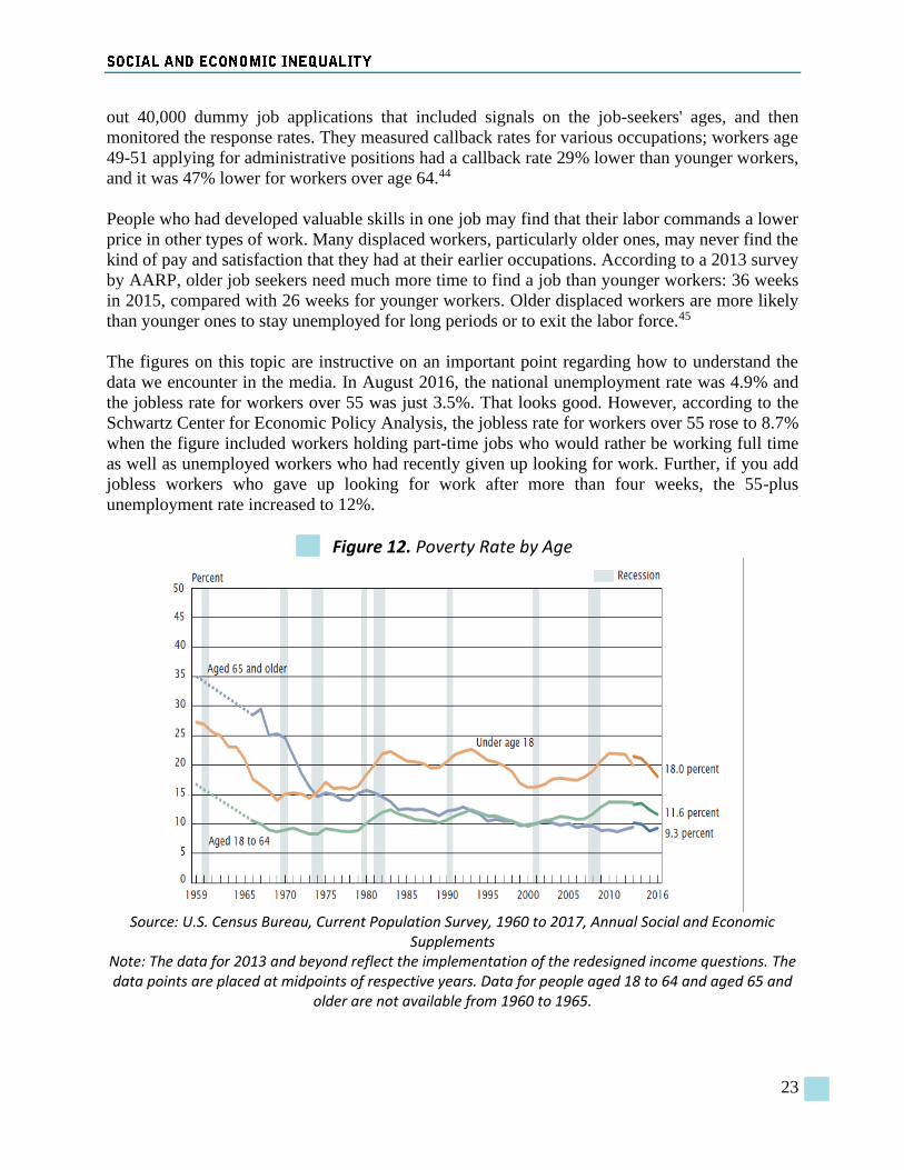
Figure 12. Poverty Rate by Age
Source: U.S. Census Bureau, Current Population Survey, 1960 to 2017, Annual Social and Economic
Supplements Note: The data for 2013 and beyond reflect the implementation of the redesigned income questions. The data points are placed at midpoints of respective years. Data for people aged 18 to 64 and aged 65 and
older are not available from 1960 to 1965.
24
Despite the difficulty older Americans have in finding jobs, poverty among the old is less
widespread than it was in the U.S. in the 1960s. (See Figure 12). This decline in poverty among
older people is largely attributed to government programs such as Social Security, Supplemental
Security Income benefits, Medicare and Medicaid. Social Security is credited for lifting about 17.1
million seniors out of poverty.46 It is important to note, however, that this poverty measure does
not consider health care costs. The high and rising medical bills for the elderly can greatly reduce
the income available to meet other basic needs. The U.S. Census Bureau also provides an
alternative measure of poverty, known as the Supplemental Poverty Measure (SPM), that takes
into consideration financial resources such as taxes, value of in-kind benefits (food stamps), and
out of pocket medical expenses. In 2016, the SPM for Americans aged 65 and older showed a
poverty rate of 14.5%, which is much higher than the official poverty rate of 9.3%.47
The Role of Education
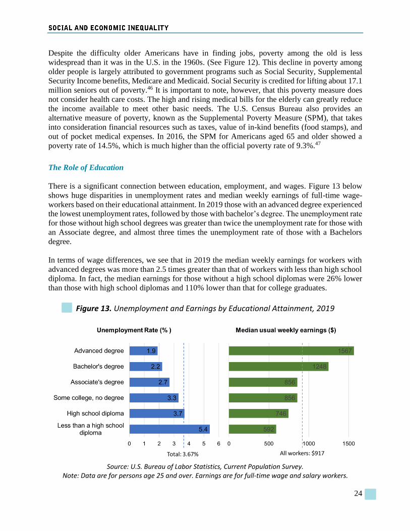
There is a significant connection between education, employment, and wages. Figure 13 below
shows huge disparities in unemployment rates and median weekly earnings of full-time wage-
workers based on their educational attainment. In 2019 those with an advanced degree experienced
the lowest unemployment rates, followed by those with bachelor’s degree. The unemployment rate
for those without high school degrees was greater than twice the unemployment rate for those with
an Associate degree, and almost three times the unemployment rate of those with a Bachelors
degree.
In terms of wage differences, we see that in 2019 the median weekly earnings for workers with
advanced degrees was more than 2.5 times greater than that of workers with less than high school
diploma. In fact, the median earnings for those without a high school diplomas were 26% lower
than those with high school diplomas and 110% lower than that for college graduates.
Figure 13. Unemployment and Earnings by Educational Attainment, 2019
Source: U.S. Bureau of Labor Statistics, Current Population Survey.
Note: Data are for persons age 25 and over. Earnings are for full-time wage and salary workers.
25
These disparities have changed significantly in recent years. From 1975 to 2014 relative wages for
those with a high school degree fell from over 80% of the amount earned by workers with at least
a college degree to less than 60%.48 Since 1980 the only group of workers whose median income
has increased are those with at least four years of college; from 1980 to 2015 the median earning
of a college-educated worker increased by 11%, from $57,764 to $64,000. Meanwhile the median
income for workers who had not completed high school dropped from $33,442 in 1980 to $25,000
in 2015, a loss of 25%.49
Level of education is not only correlated with wages, but also with another important variable—
health benefits. Across education groups, workers with a bachelor’s degree or higher level of
education are the only group that did not experience much of a decline in health insurance coverage
received through employers. Coverage fell among all other education groups. The sharpest drop
was among workers with less than a high school education, as the share of these workers with an
employer-sponsored health plan fell from 66% in 1980 to 37% in 2013.50
When the returns to work for those at the bottom of the wage distribution are particularly low,
more prime-age men in particular choose not to participate in the labor force. In recent years there
has been a decline in male workforce attachment. This decline has largely been concentrated
among those with a high school degree or less. In 1964, 98% of prime-age men with a college
degree or more participated in the workforce, compared to 97% of men with a high school degree
or less—a virtually negligible difference. In 2015, the participation rate for college-educated men
had fallen slightly to 94%, while the rate for men with a high school degree or less had plummeted
to 83%.51
4. INTERNATIONAL DATA ON INEQUALITY
4.1 Cross-Country Comparisons
We can compare the U.S. data presented so far to data on income inequality, wealth inequality,
and economic mobility in other countries. The Gini coefficient for the United States is higher than
that of all other major industrialized countries, signifying that the country has a higher degree of
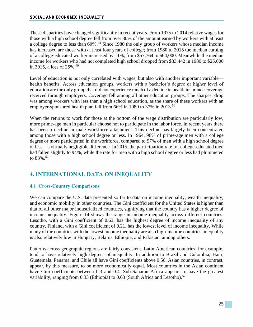
income inequality. Figure 14 shows the range in income inequality across different countries.
Lesotho, with a Gini coefficient of 0.63, has the highest degree of income inequality of any
country. Finland, with a Gini coefficient of 0.21, has the lowest level of income inequality. While
many of the countries with the lowest income inequality are also high-income countries, inequality
is also relatively low in Hungary, Belarus, Ethiopia, and Pakistan, among others.
Patterns across geographic regions are fairly consistent. Latin American countries, for example,
tend to have relatively high degrees of inequality. In addition to Brazil and Colombia, Haiti,
Guatemala, Panama, and Chile all have Gini coefficients above 0.50. Asian countries, in contrast,
appear, by this measure, to be more economically equal. Most countries in the Asian continent
have Gini coefficients between 0.3 and 0.4. Sub-Saharan Africa appears to have the greatest
variability, ranging from 0.33 (Ethiopia) to 0.63 (South Africa and Lesotho).52
26
Figure 14. Income Gini Coefficient for Select Countries
Source: CIA World Factbook, United States Central Intelligence Agency. Note: Year of data varies.
The trend toward higher income inequality is not limited to the United States. Between 1985 and
2008 income inequality increased in 17 of 22 OECD countries (it was constant in three, and
decreased in two).53 The International Monetary Fund notes that income inequality has “increased
substantially” in most developed countries since the 1990s, as well as in Asia and Eastern Europe.54
A 2012 study by the United Nations, which looked at Gini coefficient trends from the early 1990s
to 2008, found that inequality increased by 24% in China, 16% in India, and 5% in South Africa,
while inequality decreased by 9% in Brazil, along with decreases among other Latin American
countries.55 In 2015 the World Economic Forum identified income inequality as the top global
issue facing the world’s leaders in the coming years, noting that inequality “is a universal challenge
that the whole world must address.”56 Thus when we consider the causes of increasing income
inequality (in the next section) we will need to focus not just on the United States, but on broader
changes occurring across the world.
Just as with income inequality, the United States has the highest degree of wealth inequality of any
developed nation, with one report referring to the “Unequal States of America.”57 Wealth
inequality in the U.S. is higher than in many countries with very high income inequality, including
Lesotho, Colombia, and Brazil.
Finally, economic mobility appears to be lower in the United States than in nearly all other
developed nations, except for the United Kingdom and Italy, based on the strength of the
relationship between fathers’ and sons’ earnings.58 Analysis by the OECD finds a negative
correlation between income inequality and economic mobility—those countries with higher
income inequality tend to have lower economic mobility.59 The study finds that this relationship
may be linked to differences in educational opportunities. Specifically, low-income groups in
societies with high inequality tend to underinvest in education, reducing their mobility and
perpetuating inequalities. Recommended policies focus on improving access to education for low-
27
income groups, not just during youth but access to job-training and formal education throughout
one’s working life.
4.2 Global Inequality
According to the 2018 ‘World Inequality Report’, global inequality seems to have stabilized, after
widening for several decades. The share of world’s income captured by the richest 1 percent has
shrunk slightly since its peak in 2007. However, inequalities between and within countries are still
high. Between 1980 and 2016, the richest 1% of the world received 27% of the income growth,
while the bottom 50% only got 12%. The actual level of global inequality would have been even
higher, had it not been for recent rapid growth in China, moving many people in China out of
extreme poverty and toward “global middle class” status.
Just as a Gini coefficient can be calculated for an individual nation by constructing a Lorenz curve,
some economists have tried to estimate the global Gini coefficient for income. For example, a
2015 paper estimated the global Gini coefficient to be 0.65 based on 2013 data.60 Obviously, any
estimate of the global income distribution must make a number of assumptions due to the lack of
complete data, and thus different studies have resulted in slightly different global Gini coefficients.
A 2015 World Bank paper estimated the global Gini coefficient to be 0.71 in 2008,61 while a 2016
analysis produced 9 different estimates (depending on the assumptions) ranging from 0.59 to 0.61
for 2013.62 More recently, a 2019 analysis estimated the global Gini coefficient to be between 0.57
and 0.59 using 2015 data.63
Suppose the global Gini coefficient is around 0.60. If we compare this with the values in Figure
14 we notice that the global Gini coefficient is higher than that for almost every individual country.
While you might expect that the global Gini coefficient would be approximately an average of the
coefficients for each country, this is clearly not true. How can it be that the global Gini coefficient
is higher than the value for nearly all countries?
To resolve this seeming paradox, we must realize that the incomes found in most countries do not
cover the full range from the world’s poorest to the world’s richest. For example, in many
developed countries such as Germany and Switzerland there are virtually no people living below
the World Bank’s measure of absolute poverty of $1.90 per day. The United States is an exception;
the World Bank estimates that more than 3 million Americans live below the global poverty line.64
In Lesotho—the country with the highest income Gini coefficient—about 60% of the population
lives in absolute poverty, and income per capita is only about $1,300 per year.65 So even those
with relatively high incomes in Lesotho may not be particularly rich by global standards. But when
we calculate the global Gini coefficient we bring together all the world’s incomes, comparing the
800 million living in absolute poverty to the 5 million or so making more than $1 million per
year.66
Another way to understand the extremely unequal global income distribution is to consider what
income is necessary to reach various percentiles. According to the online Global Rich List
calculator, an annual income of only about $7,000 is needed to make it into the top global
quintile.67 And an annual income of only $33,000 puts you in the global top 1%. So an American
worker making a median U.S. wage of around $48,000 per year is well into the global top 1%.68
28
In other words, the country in which one is born largely determines one’s economic fate.69 Some
scientists refer to a global “birth lottery,” whereby if:
you are lucky enough to be born in a wealthy country, you will more likely enjoy
the great fortunes and opportunities that come from being a citizen of that country.
Conversely, if you “lose” the birth lottery, and you are born in a poor country, your
life chances and circumstances will mostly likely suffer accordingly.70
As mentioned previously, income inequality is increasing in most countries, including China,
India, and most developed nations. You might then conclude that the global Gini coefficient is also
increasing. However, various studies conclude that global income inequality is decreasing in recent
decades.71
How can the Gini coefficient for most countries be increasing, while the global Gini coefficient is
declining? Essentially, the growth of the global middle class is reducing global inequality even as
it increases national-level inequality in many countries. Consider that several decades ago nearly
all people in China and India—the world’s two most populous countries—had very low incomes
by global standards. Recent economic growth in these countries has increased national level
inequality, specifically between relatively high incomes in urban areas and the still-low incomes
in rural areas. But economic growth in these two countries has led to a surge in the number of
people classified in the global middle class. This emerging global middle class is reducing global
inequality.
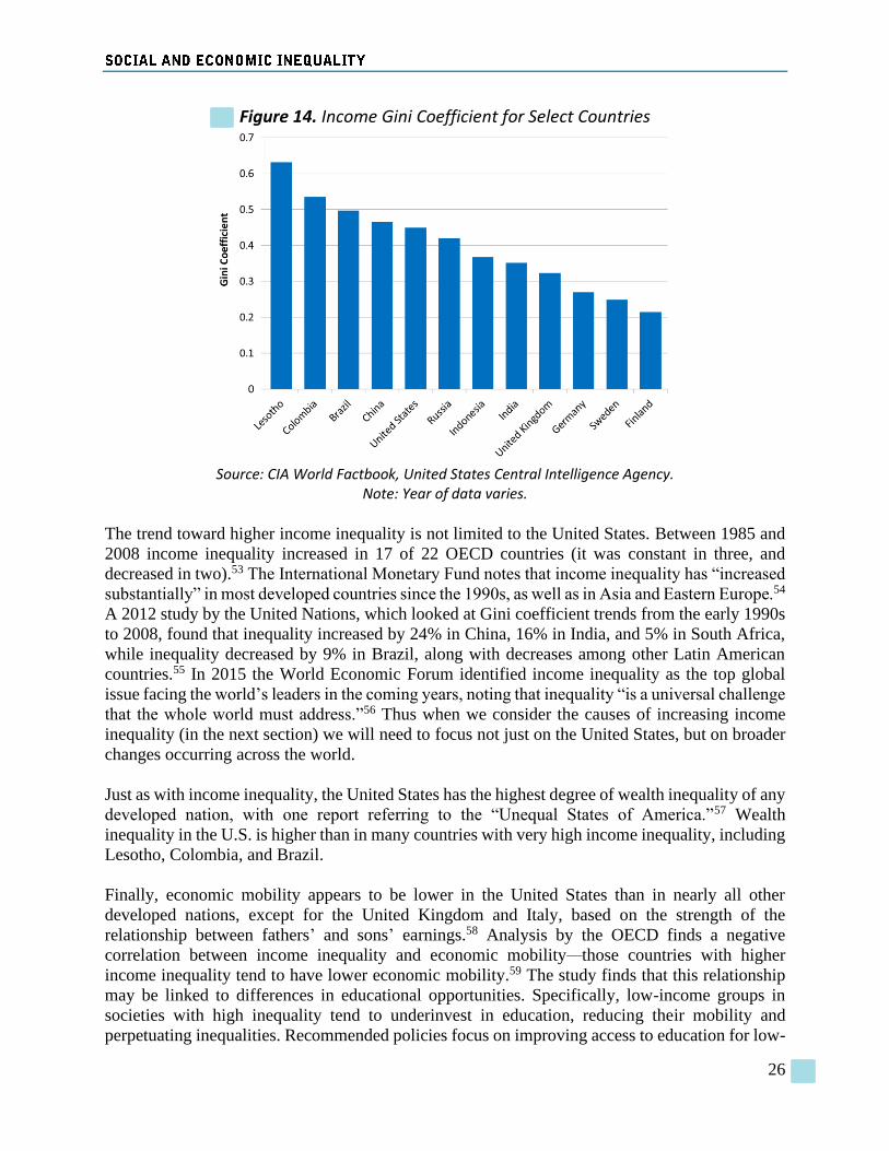
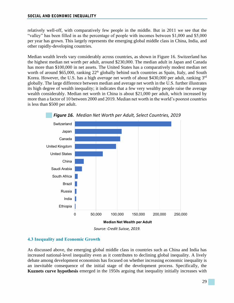
Figure 15. Global Income Distribution, 1988 and 2011
Source: Our World in Data website, https://ourworldindata.org/income-inequality/
We can see evidence of this shift in Figure 15, which shows the global distribution of income in
1988 and 2011. Note that this income distribution graph is different from our Lorenz curve graphs,
as the y-axis shows shares of the world’s population at various income levels, and the x-axis
presents income levels using a nonlinear scale. In 1988 we see a distribution with two “peaks”:
one around a few hundred dollars per person per year and another around $10,000. Thus there
were two large concentrations of people in 1988—those who were very poor and those who were
1. What are some of the differences between inequality of income and inequality of
“capabilities” or well-being? How are these concepts related? Which one do you think
deserves more attention from policymakers?
2. What do you think is the minimal amount of annual income that an individual, or a small
family, would need to live in your community? (Think about the rent or mortgage on a one-
or two-bedroom residence, etc.) What does this probably mean about where the average
level of income in your community fits into the U.S. income distribution shown in Table
1?
3. Were your parents better off economically than their parents? Do you believe that you will
be better off than your parents? Do you think that this is true of most of your friends?
4. Make a list of the reasons that inequality can be considered desirable, and the ways in
which inequality hurts social well-being. Is it possible to limit the negative consequences
of inequality while still harnessing the positive aspects?
5. What do you think are the reasons that the United States is more unequal than other
developed countries, and has lower economic mobility? What policies might be used to
address this issue?
6. What are the main trends in global inequality? Do these seem to be positive or negative in
terms of human well-being?
7. If you could change a single one of the “causes” of inequality described above, on which
would you choose to focus? Why?
8. Do you think rising inequality in a rapidly developing low-income country is necessarily a
problem? How might you approach the issue of high economic inequality differently in a
developing versus a developed country?
9. Do you generally believe that raising taxes on the rich is an appropriate approach for
reducing economic inequality? What level of taxation on the rich do you think is fair?
10. Do you think the spending priorities of the government should be changed in order to
reduce economic inequality? Beyond the suggestions in the text, can you think of any other
ways that government spending priorities could be changed?
54
Notes 1 Saez, 2016. 2 Dabla-Norris et al., 2015. 3 Dickman et al., 2017. 4 Data from the United Nations Development Programme, Human Development Reports database. 5 Reardon, 2012. 6 World Economic Forum, 2016. 7 IGM Forum, 2020.
8 Zeballos-Roig, 2020. 9 US BLS, 2019. 10 US BLS, 2020a. 11 US BLS, 2020b. 12 Pilkington, 2020. 13 Ostry, et al., 2020. 14 Gerszon-Mahler, et al., 2020. 15 Ostry, et al., 2020. 16 Godwin and Tokunbor, 2016. 17 Vidal, 2013. 18 Burke et al., 2015. 19 Anonymous, 2014. 20 Brandmeir et al., 2016. 21 Saez and Zucman, 2016. 22 Norton and Ariely. 2011. 23 Note that the “actual” distribution of wealth in Figure 8 differs somewhat from the distribution given in Figure
7—the two figures rely upon different data sources and apply to different years. 24 Norton and Ariely, 2011, p. 12. 25 Ibid. 26 Note that the categories presented in Figures 6 and 9 slightly differ, as the data come from two different U.S.
Census Bureau reports. 27 Bengali and Daly, 2013. 28 The Pew Charitable Trusts and the Russell Sage Foundation, 2015, p. 5. 29 Carr and Wiemers, 2016. 30 Chetty et al., 2017. 31 Ibid, p. 9. 32 Quillian et al., 2017. 33 Fryer et al., 2013. 34 Wilson and Rodgers, 2016. 35 Brown and Patten, 2017. 36 Blau and Kahn, 2016. 37 Oyedele, 2016. 38 World Economic Forum, 2016. 39 Pew Research Center, 2015. 40 Pew Research Center, October 2016. Note that annual earning is expressed in 2014 dollars. 41 BLS News Release, October 2017. 42 Porter, 2017. 43 BLS News Release, October 2017. 44 Neumark et al., 2015. 45 Koenig et al., 2015. 46 Kadlec, 2016 47 U.S. Census, 2018. 48 CEA, 2016. 49 Pew Research, October 2016. 50 Ibid.
55
51 CEA, 2016. 52 All Gini coefficients from the CIA World Factbook. 53 OECD, 2011. 54 Dabla-Norris et al., 2015. 55 Vieira, 2012. 56 http://reports.weforum.org/outlook-global-agenda-2015/top-10-trends-of-2015/1-deepening-income-inequality/. 57 Brandmeir et al., 2016. 58 Corak, 2016. 59 OECD, 2015. 60 Hellebrandt and Mauro, 2015. 61 Lakner and Milanovic, 2015. 62 Darvas, 2016. 63 Darvas, 2019. 64 Deaton, 2018. 65 http://povertydata.worldbank.org/poverty/country/LSO. 66 Absolute poverty estimate from the World Bank (http://www.worldbank.org/en/topic/poverty/overview). High-
income estimate from the Global Rich List (http://www.globalrichlist.com/). 67 http://www.globalrichlist.com/. 68 Median wage data from the U.S. Bureau of Labor Statistics, Economic News Release, Table 1. Median usual
weekly earnings of full-time wage and salary workers by sex, quarterly averages, seasonally adjusted, fourth quarter
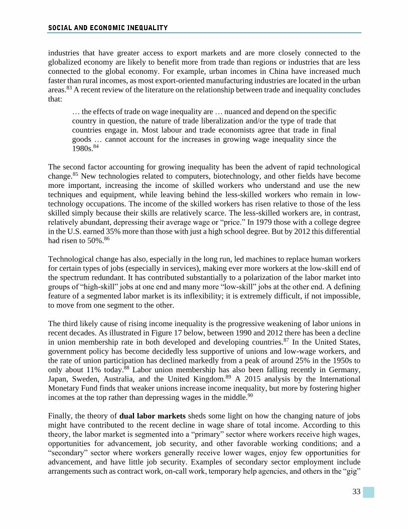
2019. 69 See Milanovic, 2015. 70 Kaufman, 2015. 71 Anonymous, 2012. 72 Moran, 2005. 73 Moran, 2005; Wade, 2011. 74 Kanbur et al., 2017. 75 Greenwood et al., 2014. 76 Olson, 1984. 77 IMF, 2017. 78 Federal Reserve Bank of St. Louis online database, https://fred.stlouisfed.org/series/LES1252881600Q. 79 Federal Reserve Bank of St. Louis online database, https://fred.stlouisfed.org/series/A939RX0Q048SBEA. 80 Krugman, 2008. 81 Keller and Olney, 2017. 82 Pavcnik, 2017. 83 OECD, 2015 (c). 84 Pavcnik, 2011. 85 Pavcnik, 2011. 86 Rotman, 2014. 87 Emerging markets include Brazil, Chile, China, India, Indonesia, Korea, Mexico, Philippines, Russia, South
Africa, Thailand, and Turkey. 88 U.S. Bureau of Labor Statistics, 2017b. 89 OECD online statistics, trade union density. 90 Jaumotte and Buitron, 2015. 91 NACo, 2017. 92 Alderman, 2017. 93 Tax Policy Center, 2017. 94 Piketty and Saez, 2007. 95 Dabla-Norris et al., 2015. 96 Obst, 2013. 97 Schmitt, 2009, p. 3-4. 98 Santiago et al., 2011. 99 Wilkinson and Pickett, 2009. 100 Sanandaji et al., 2010. 101 Deaton, 2003. 102 Ostry et al., 2014.
103 Ibid, p. 25. 104 Ibid, p. 26. 105 Gilens, 2012. 106 Ibid, p. 1. 107 Piketty and Saez, 2007. 108 Feenberg et al., 2017. 109 OECD, 2008. 110 Joumard et al., 2012. 111 OECD, 2011. 112 Autor et al., 2016. 113 OECD, 2012. 114 Neumark, 2014. 115 Harris and Kearney, 2014. 116 Cooper, 2017. 117 See http://worksite.actu.org.au/youth-entry-level-wages/. 118 Breen and Chung, 2015. 119 Hershbein et al., 2015. 120 Jaumotte and Buitron, 2015. 121 Checchi and van de Werfhorst, 2014. 122 Haarmann and Haarmann, 2014. 123 Reuters, 2019. Data on average unemployment benefits is from the Finnish Social Security (Kela) website
(www.kela.fi). 124 Goodman, 2017. 125 Jaumotte and Buitron, 2015. 126 Matthews, 2012. 127 OECD, 2012. 128 Ambrosino, 2016. 129 See https://projects.propublica.org/graphics/temps-around-the-world. 130 Ravallion, 2014. 131 UNDP, 2013. 132 Lin and Yun, 2016. 133 Shimeles, 2016. 134 See http://www.worldbank.org/en/news/opinion/2013/11/04/bolsa-familia-Brazil-quiet-revolution. 135 Hall, 2014. 136 OECD, 2015b.