Institute for Advanced Development Studies

Development Research Working Paper Series

No. 09/2010

Social Impacts of Climate Change in Mexico: A municipality level analysis of the effects of recent and future climate change on human development

and inequality

by:

Lykke E. Andersen Dorte Verner

July 2010 The views expressed in the Development Research Working Paper Series are those of the authors and do not necessarily reflect those of the Institute for Advanced Development Studies. Copyrights belong to the authors. Papers may be downloaded for personal use only.

1

Social Impacts of Climate Change in Mexico:

A municipality level analysis of the effects of recent and future climate change on human development and

inequality*

by

Lykke E. Andersen

Dorte Verner

July, 2010

Summary:

This paper uses municipality level data to estimate the general relationships

between climate, income and child mortality in Mexico. Climate was found to

play only a very minor role in explaining the large differences in income

levels and child mortality rates observed in Mexico. This implies that Mexico

is considerably less vulnerable to expected future climate change than other

countries in Latin America.

Keywords: Climate change, social impacts, Mexico.

JEL classification: Q51, Q54, O15, O19, O54.

* This paper forms part of the World Bank research project ―Social Impacts of Climate Change and

Environmental Degradation in the LAC Region.‖ Financial support from the Danish Development Agency

(DANIDA) is gratefully acknowledged. The meticulous research assistance of Soraya Román is greatly

appreciated, as are the comments and suggestions received from Kirk Hamilton, Jacoby Hanan, and John

Nash.The findings, interpretations, and conclusions expressed in this paper are those of the authors and do not

necessarily reflect the views of the Executive Directors of The World Bank or the governments they

represent. Institute for Advanced Development Studies, La Paz, Bolivia. Please direct correspondence concerning this paper to landersen@inesad.edu.bo. The World Bank, Washington, DC.

2

1. Introduction and justification

A simple way to gauge how climate change affects human development is to compare

human development across regions with different climates. This has, for example, been

done by Horowitz (2006), which uses a cross-section of 156 countries to estimate the

relationship between temperature and income level. The overall relationship found is very

strongly negative, with a 2F increase in global temperatures implying a 13% drop in

income. This is very dramatic, but the relationship is thought to be mostly historical and

thus not very relevant for the prediction of the effects of future climate change. In order to

control for historical factors, the paper includes colonial mortality rates as an explanatory

variable, and finds a much more limited, but still highly significant, contemporaneous

effect of temperature on incomes. The contemporaneous relationship estimated implies that

a 2F increase in global temperatures would cause approximately a 3.5% drop in World

GDP.

In order to further control for historical differences, Horowitz (2006) uses more

homogeneous sub-samples, such as only OECD countries or only countries from the

Former Soviet Union, and the negative relationship still holds. However, as directions for

further research, he recommends empirical studies of income and temperature variations

within large, heterogeneous countries, which would provide much more thorough control

for historical differences.

This is exactly what we will do in the present paper. Using data from 2443 municipalities in

Mexico, we will estimate contemporary relationships between temperature and income as

well as between temperature and child mortality. While it is always dangerous to make

inferences about changes in time from cross-section estimates, these relationships can at

least be used to gauge the likely direction and magnitude of effects of climate change in

Mexico.

Two different types of climate change will be assessed. First, the documented recent

climate change in each of the 2443 municipalities, as estimated from average monthly

temperature series from 1948 to 2008 for all the Mexican meteorological stations that have

contributed systematically to the Monthly Climatic Data for the World (MCDW)

publication of the US National Climatic Data Center.

Second, we will use the predictions of the Fourth Assessment Report of the

Intergovernmental Panel on Climate Change (IPCC4) climate models to simulate the likely

effects of projected future climate change in Mexico.

The rest of the paper is organized as follows. Section 2 describes the data sources and

provides descriptions of the key variables. Section 3 estimates the cross-municipality

relationships between climate and human development, controlling for other key variables

that also affect development. Section 4 analyzes past climate change for 22 meteorological

stations across Mexico, and estimates average trends in temperatures and precipitation.

Section 5 uses the results from sections 3 and 4 to simulate the effects of climate change on

3

income and child mortality in each of the 2350 municipalities in Mexico.. Section 6

concludes.

2. The data

The data used for this paper consists of both cross-section data and time series data. The

municipality level cross-section data base which was used to estimate the relationship

between climate and development in Mexico was constructed using data from many

different sources. Table 1 lists the variables, their definitions, and the sources of the

information.

Table 1: Variables in the municipality level data base for Mexico

Variable Unit Source

Total population per municipality - Municipal Human

Development Index – PNUD Mexico 2000

Urbanization rate

(Percentage of population living in urban areas)

% Municipal Human

Development Index – PNUD Mexico 2000

Literacy rate

(Percentage of the adult population

that can read and write)

% Municipal Human

Development Index –

PNUD Mexico 2000

Child mortality Deaths per 1000

live births

Municipal Human

Development Index –

PNUD Mexico 2000

Per capita income PPP-adjusted US$

Municipal Human Development Index –

PNUD Mexico 2000

Latitude Decimal degrees Google Earth

Longitude Decimal degrees Google Earth

Elevation Kilometers

above sea level

Google Earth

Normal average annual temperature Degrees Celsius Servicio Meteorológico

Nacional

Normal annual rainfall Milimeters Servicio Meteorológico

Nacional

In order to assess the climate change trends in the different parts of Mexico, we obtained

monthly temperature and rainfall data from 1948 to 2008 from the Monthly Climatic Data

for the World (MCDW) publication of the US National Climatic Data Center (NCDC).

This data is described in more detail in Section 4 below.

4

3. Modeling climate and human development

In this section, we will estimate the contemporary relationship between climate and human

development in Mexico. Two dimensions of human development will be analyzed: income

and health, because these are the ones that most directly could be affected by climate

change. Education, on the other hand, is treated as an explanatory variable instead of a

dependent variable. In order to obtain a contemporary relationship relevant for the

simulation of the impacts of climate change over the past 50 years and future 50 years, we

need to control for other variables that also affect human development, but are likely not

affected by climate change within this time frame. Education level is by far the most

important control variable, as it explains a very high percentage of the variation in both

income and child mortality across municipalities (see below), and the progress achieved in

the area of education is not likely to be compromised because of the modest climate

changes that are expected within the next 50 years. The urbanization rate is another

important control variable, which clearly affects both income and child mortality, but which

is relatively unaffected by climate change in the short run (50 years).

As several researchers have pointed out, the relationship between temperature and

development is likely to be hump-shaped, as both too cold and too hot climates may be

detrimental for human development (Mendelsohn, Nordhaus & Shaw, 1994; Quiggin &

Horowitz, 1999; Masters & McMillan, 2001, Tol, 2005). In order to allow for this

possibility we include both average annual temperature and its square in the regression. The

same argument also holds for rainfall and possibly also urbanization rates, which is why we

also include rainfall and urbanization rates squared.

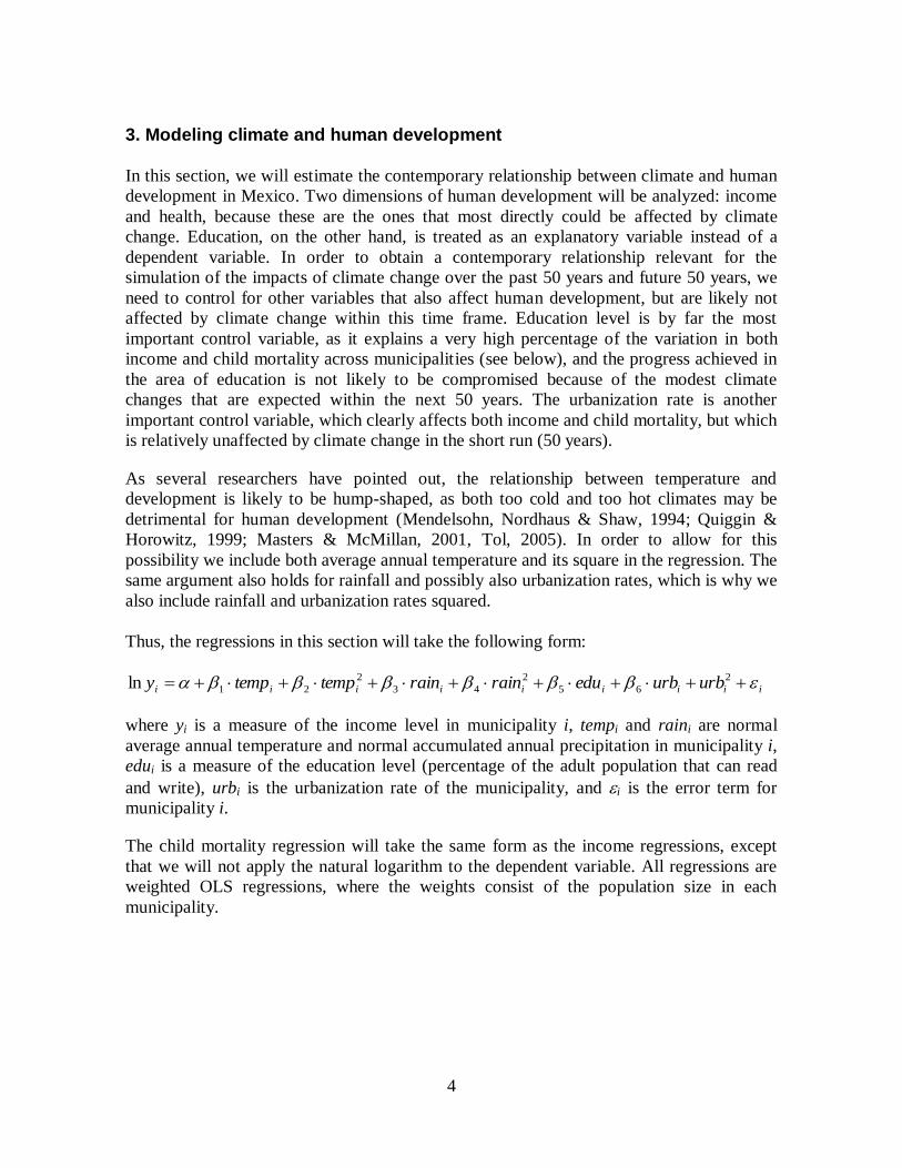
Thus, the regressions in this section will take the following form:

iiiiiiiii urburbedurainraintemptempy 2

65

2

43

2

21ln

where yi is a measure of the income level in municipality i, tempi and raini are normal

average annual temperature and normal accumulated annual precipitation in municipality i,

edui is a measure of the education level (percentage of the adult population that can read

and write), urbi is the urbanization rate of the municipality, and i is the error term for

municipality i.

The child mortality regression will take the same form as the income regressions, except

that we will not apply the natural logarithm to the dependent variable. All regressions are

weighted OLS regressions, where the weights consist of the population size in each

municipality.

5

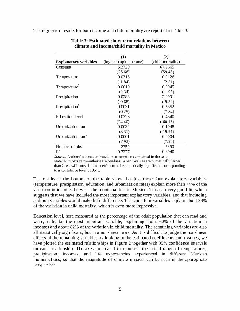
The regression results for both income and child mortality are reported in Table 3.

Table 3: Estimated short-term relations between

climate and income/child mortality in Mexico

Explanatory variables

(1)

(log per capita income) (2)

(child mortality)

Constant 5.3729 (25.66)

67.2665 (59.43)

Temperature -0.0313

(-1.84)

0.2126

(2.31)

Temperature2 0.0010

(2.34) -0.0045 (-1.95)

Precipitation -0.0283

(-0.68)

-2.0991

(-9.32) Precipitation

2 0.0031

(0.25)

0.5352

(7.84)

Education level 0.0326

(24.40)

-0.4340

(-60.13) Urbanization rate 0.0032

(3.31)

-0.1048

(-19.91)

Urbanization rate2

0.0001 (7.92)

0.0004 (7.96)

Number of obs. 2350 2350

R2 0.7377 0.8940

Source: Authors’ estimation based on assumptions explained in the text.

Note: Numbers in parenthesis are t-values. When t-values are numerically larger

than 2, we will consider the coefficient to be statistically significant, corresponding

to a confidence level of 95%.

The results at the bottom of the table show that just these four explanatory variables

(temperature, precipitation, education, and urbanization rates) explain more than 74% of the

variation in incomes between the municipalities in Mexico. This is a very good fit, which

suggests that we have included the most important explanatory variables, and that including

addition variables would make little difference. The same four variables explain about 89%

of the variation in child mortality, which is even more impressive.

Education level, here measured as the percentage of the adult population that can read and

write, is by far the most important variable, explaining about 62% of the variation in

incomes and about 82% of the variation in child mortality. The remaining variables are also

all statistically significant, but in a non-linear way. As it is difficult to judge the non-linear

effects of the remaining variables by looking at the estimated coefficients and t-values, we

have plotted the estimated relationships in Figure 2 together with 95% confidence intervals

on each relationship. The axes are scaled to represent the actual range of temperatures,

precipitation, incomes, and life expectancies experienced in different Mexican

municipalities, so that the magnitude of climate impacts can be seen in the appropriate

perspective.

6

Panel (a) shows an almost flat relationship between temperature and per capita income.

There is a tremendous variation in incomes between municipalities, but this variation has

little to do with average temperatures.

Panel (b) also shows an almost completely flat relationship between temperature and child

mortality.

Figure 2: Estimated contemporary relations between

temperature/rainfall and income/child mortality in Mexico

(a) Temperature and Income

148

5148

10148

15148

20148

25148

30148

35148

8 10 12 14 16 18 20 22 24 26 28 30

Inco

me

pe

r ca

pita

(P

PA

-$/Y

ea

r)

Average annual temperature (ºC)

(b) Temperature and child mortality

17

22

27

32

37

42

47

52

57

62

67

8 10 12 14 16 18 20 22 24 26 28 30

Ch

ild

mo

rta

lity

(p

er

10

00

liv

e b

irth

s)

Average annual temperature (ºC)

(c) Rainfall and Income

148

5148

10148

15148

20148

25148

30148

35148

0 1 2 3 4 5 6

Inco

me

pe

r ca

pita

(P

PA

-$/Y

ea

r)

Accumulated annual precipitation (m)

(d) Rainfall and child mortality

17

22

27

32

37

42

47

52

57

62

67

0 1 2 3 4 5 6

Ch

ild

mo

rta

lity

(p

er

10

00

liv

e b

irth

s)

Accumulated annual precipitation (m)

Source: Graphical representation of the estimation results from Table 3. The thick red line represents the point estimate, while the thin black lines delimit the 95% confidence interval as estimated by Stata’s lincom command.

7

The only statistically significant climate-development relationship found for Mexico is

shown in panel (d) which suggests that child mortality is lowest in regions with moderate

amounts of rainfall, and higher in regions with either very little or very much rain.

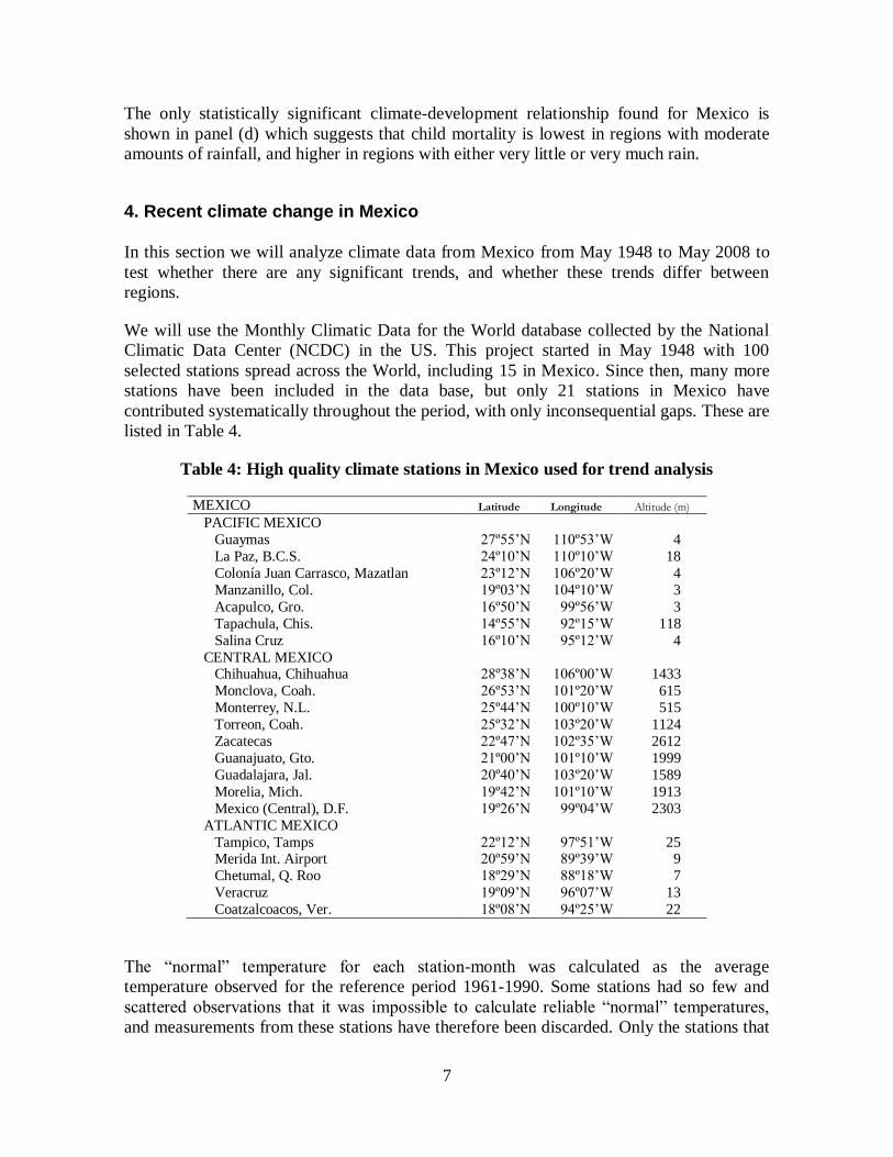
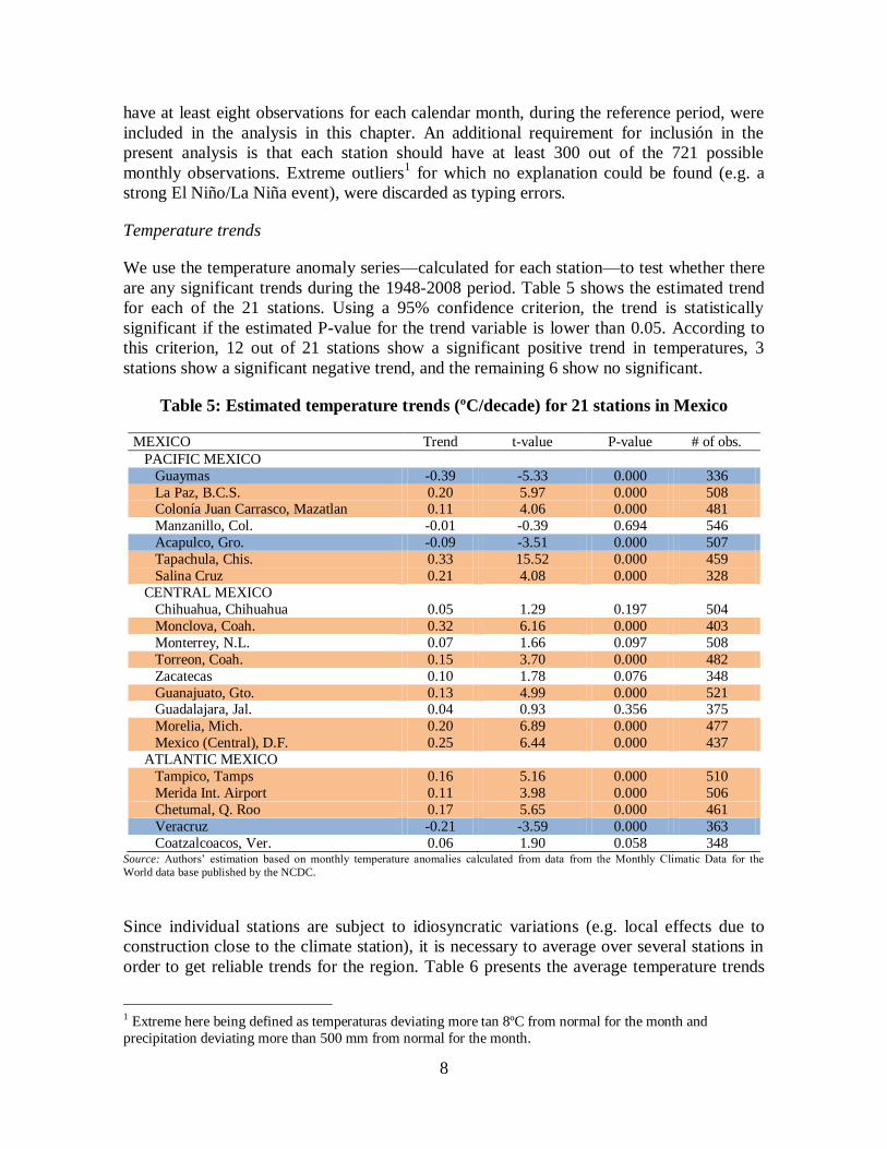
4. Recent climate change in Mexico

In this section we will analyze climate data from Mexico from May 1948 to May 2008 to

test whether there are any significant trends, and whether these trends differ between

regions.

We will use the Monthly Climatic Data for the World database collected by the National

Climatic Data Center (NCDC) in the US. This project started in May 1948 with 100

selected stations spread across the World, including 15 in Mexico. Since then, many more

stations have been included in the data base, but only 21 stations in Mexico have

contributed systematically throughout the period, with only inconsequential gaps. These are

listed in Table 4.

Table 4: High quality climate stations in Mexico used for trend analysis

MEXICO Latitude Longitude Altitude (m)

PACIFIC MEXICO

Guaymas 27º55’N 110º53’W 4

La Paz, B.C.S. 24º10’N 110º10’W 18

Colonía Juan Carrasco, Mazatlan 23º12’N 106º20’W 4

Manzanillo, Col. 19º03’N 104º10’W 3

Acapulco, Gro. 16º50’N 99º56’W 3

Tapachula, Chis. 14º55’N 92º15’W 118

Salina Cruz 16º10’N 95º12’W 4

CENTRAL MEXICO Chihuahua, Chihuahua 28º38’N 106º00’W 1433

Monclova, Coah. 26º53’N 101º20’W 615

Monterrey, N.L. 25º44’N 100º10’W 515

Torreon, Coah. 25º32’N 103º20’W 1124

Zacatecas 22º47’N 102º35’W 2612

Guanajuato, Gto. 21º00’N 101º10’W 1999

Guadalajara, Jal. 20º40’N 103º20’W 1589

Morelia, Mich. 19º42’N 101º10’W 1913

Mexico (Central), D.F. 19º26’N 99º04’W 2303

ATLANTIC MEXICO

Tampico, Tamps 22º12’N 97º51’W 25 Merida Int. Airport 20º59’N 89º39’W 9

Chetumal, Q. Roo 18º29’N 88º18’W 7

Veracruz 19º09’N 96º07’W 13

Coatzalcoacos, Ver. 18º08’N 94º25’W 22

The ―normal‖ temperature for each station-month was calculated as the average

temperature observed for the reference period 1961-1990. Some stations had so few and

scattered observations that it was impossible to calculate reliable ―normal‖ temperatures,

and measurements from these stations have therefore been discarded. Only the stations that

8

have at least eight observations for each calendar month, during the reference period, were

included in the analysis in this chapter. An additional requirement for inclusión in the

present analysis is that each station should have at least 300 out of the 721 possible

monthly observations. Extreme outliers1 for which no explanation could be found (e.g. a

strong El Niño/La Niña event), were discarded as typing errors.

Temperature trends

We use the temperature anomaly series—calculated for each station—to test whether there

are any significant trends during the 1948-2008 period. Table 5 shows the estimated trend

for each of the 21 stations. Using a 95% confidence criterion, the trend is statistically

significant if the estimated P-value for the trend variable is lower than 0.05. According to

this criterion, 12 out of 21 stations show a significant positive trend in temperatures, 3

stations show a significant negative trend, and the remaining 6 show no significant.

Table 5: Estimated temperature trends (ºC/decade) for 21 stations in Mexico

MEXICO Trend t-value P-value # of obs.

PACIFIC MEXICO

Guaymas -0.39 -5.33 0.000 336

La Paz, B.C.S. 0.20 5.97 0.000 508 Colonía Juan Carrasco, Mazatlan 0.11 4.06 0.000 481

Manzanillo, Col. -0.01 -0.39 0.694 546

Acapulco, Gro. -0.09 -3.51 0.000 507

Tapachula, Chis. 0.33 15.52 0.000 459

Salina Cruz 0.21 4.08 0.000 328

CENTRAL MEXICO

Chihuahua, Chihuahua 0.05 1.29 0.197 504

Monclova, Coah. 0.32 6.16 0.000 403

Monterrey, N.L. 0.07 1.66 0.097 508

Torreon, Coah. 0.15 3.70 0.000 482

Zacatecas 0.10 1.78 0.076 348

Guanajuato, Gto. 0.13 4.99 0.000 521

Guadalajara, Jal. 0.04 0.93 0.356 375

Morelia, Mich. 0.20 6.89 0.000 477

Mexico (Central), D.F. 0.25 6.44 0.000 437

ATLANTIC MEXICO

Tampico, Tamps 0.16 5.16 0.000 510

Merida Int. Airport 0.11 3.98 0.000 506

Chetumal, Q. Roo 0.17 5.65 0.000 461

Veracruz -0.21 -3.59 0.000 363

Coatzalcoacos, Ver. 0.06 1.90 0.058 348

Source: Authors’ estimation based on monthly temperature anomalies calculated from data from the Monthly Climatic Data for the

World data base published by the NCDC.

Since individual stations are subject to idiosyncratic variations (e.g. local effects due to

construction close to the climate station), it is necessary to average over several stations in

order to get reliable trends for the region. Table 6 presents the average temperature trends

1 Extreme here being defined as temperaturas deviating more tan 8ºC from normal for the month and

precipitation deviating more than 500 mm from normal for the month.

9

by climatic region. According to this table, the central zone of Mexico is warming about 3

times faster than the coastal zones. The estimated trends correspond to a change over 50

years of about 0.25ºC in the coastal regions and 0.75ºC in the central region.

Table 6: Estimated temperature trends (ºC/decade) for the 3 main climate regions in

Mexico

Trends Average Maximum Minimum

PACIFIC ZONE 0.0514 0.3300 -0.3900

CENTRAL ZONE 0.1456 0.3200 0.0400

ATLANTIC ZONE 0.0580 0.1700 -0.2100

Precipitation trends

Precipitation varies tremendously across Mexico. The Sonoran desert in the Northwest

receives less than 10 cm of rain per year, while the tropical rainforest of southern Mexico

receives more than 2 meters of rain annually. The wettest place, San Juan Comaltepec in

Oaxaca, receives 6.1 meters of precipitation annually. According to Liverman (1999), the

various climates of Mexico are determined by the latitudinal belts of atmospheric

circulation which shift seasonally and include the westerlies which bring precipitation to

northern Mexico in winter, the sub-tropical highs associated with stable, dry conditions,

and the trade winds which bring summer rainfall to the central and southern regions of the

country. Precipitation is also affected by fall hurricanes on both the Caribbean and Pacific

coasts and summer monsoons in the north. The mountainous topography of Mexico is also

of key importance, creating rain shadows behind coastal mountains.

Small shifts in the natural paths of fall hurricanes and summer monsoons can create large

inter-annual variation in precipitation, which means that precipitation in any specific place

is very variable.

A trend analysis, however, reveals no systematic changes in rainfall over the period 1948-

2008. All stations except one show no significant trend in monthly precipitation anomalies

(see Table 7). We will therefore conclude that there have been no systematic changes in

precipitation in Mexico during the last 6 decades.

Table 7: Estimated precipitation trends (ºC/decade) for 19 stations in Mexico

MEXICO Trend t-value P-value # of obs.

PACIFIC MEXICO

Guaymas 1.26 1.22 0.223 295

Colonía Juan Carrasco, Mazatlan -0.64 -0.34 0.737 453

Manzanillo, Col. 1.90 0.90 0.370 512

Acapulco, Gro. -0.84 -0.33 0.741 473

Tapachula, Chis. -0.39 -0.16 0.876 430

Salina Cruz -0.57 -0.19 0.846 300

CENTRAL MEXICO

Chihuahua, Chihuahua -1.06 -1.01 0.315 477

Monterrey, N.L. 1.34 0.87 0.382 495

Torreon, Coah. 0.01 0.01 0.993 444

10

Zacatecas -0.45 -0.27 0.789 331

Guanajuato, Gto. 0.07 0.04 0.964 502

Guadalajara, Jal. 0.89 0.55 0.585 371

Morelia, Mich. 0.85 0.76 0.445 466

Mexico (Central), D.F. 0.04 0.03 0.973 423

ATLANTIC MEXICO

Tampico, Tamps 2.26 1.12 0.263 493

Merida Int. Airport 1.57 0.87 0.387 500

Chetumal, Q. Roo 4.39 2.03 0.043 441

Veracruz -0.62 -0.20 0.838 341

Coatzalcoacos, Ver. -1.93 -0.50 0.615 334

Source: Authors’ estimation based on monthly precipitation anomalies calculated from data from the Monthly Climatic Data for the

World data base published by the NCDC.

5. Simulating the impacts of climate change

In this section, we planned to use the two models estimated in Table 3 above to simulate the

impacts of the climate change experienced during the last 50 years on per capita income

and child mortality in each of the 2443 municipalities in Mexico.

However, since income and child mortality were not found to be significantly related to

temperatures, and since precipitation does not seem to have changed systematically over

the last 50 years, there is nothing left to simulate, and our conclusion must be that the

gradual climate change experienced over the last 50 years has not had a statistically

significant effect on neither incomes nor child mortality in Mexico.

Notice, however, that we are only talking about systematic climate change (i.e. the slight

temperature increases of 0.25ºC-0.75ºC), not extreme events.

In terms of the effect of future climate change, there is a potential impact on child mortality

from changes in precipitation. Most of the models in the IPCC ensemble of 21 Atmosphere-

Ocean General Circulation Models suggest precipitation reductions over the coming

decades, but at least a handful of models show increases, which means that future changes

are highly uncertain (see Figure 5). In the simulations of the effects on child mortality we

will assume modest reductions of 5% over the next 50 years all over Mexico.

Figure5: Temperature and precipitation changes predicted by the climate models

used by IPCC 4, 1990-2090

11

Source: Christensen et al (2007, Figure 11.12).

To find the impacts of climate change we will compare the following two scenarios: 1)

Climate Change and 2) No Climate Change, where the only difference between the two are

in the climate variables. The Climate Change level of child mortality can be written as:

iij

k

j

jiiCCiCCiCCi XrrttCM ˆˆˆˆˆˆ,

1

2

43

2

,2,1,

,

where the index i refers to municipality i; t and r are the temperature and precipitation

variables; the s are the estimated coefficients on the temperature and precipitation

variables; the Xjs are the remaining j explanatory variables including the constant term; the

j s are the coefficient to these variables; and i are the estimated error terms for each

municipality.

Equivalently, the counterfactual level of child mortality under the assumption of No

Climate Change can be written as:

12

iij

k

j

jiiNCCiNCCiNCCi XrrttCM ˆˆˆˆˆˆ,

1

2

43

2

,2,1,

,

where only the climate variables differ.

The difference between the two scenarios is the difference in child mortality that can be

directly attributed to climate change:

)(ˆ)(ˆ

)(ˆ)(ˆ

2

,

2

,4,,3

2

,

2

,2,,1,,

NCCiCCiNCCiCCi

NCCiCCiNCCiCCiNCCiCCiiCC

rrrr

ttttCMCMCM

Since the coefficients 1 and 2 were found to be statistically indifferent from zero,

however, this relationship reduces to:

)(ˆ)(ˆ 2

,

2

,4,,3,, NCCiCCiNCCiCCiNCCiCCiiCC rrrrCMCMCM

At the aggregate level, future climate change in Mexico is estimated to cause a small

increase in average child mortality of about 0.07 deaths per thousand live births. The most

adverse effect found in any municipality was an increase of 0.24 while the most beneficial

effect was a reduction of 1.25 deaths per 1000 live births. Thus, the expected effect of

future climate change on child mortality is minimal.

6. Conclusions

In this paper we used a municipal level cross-section database to estimate the cross-

sectional relationships between climate and income/child mortality in Mexico. We found

that average temperatures and average precipitation are not significantly related to income.

Only the relationship between precipitation and child mortality was found to be statistically

significant, with higher child mortality rates in regions with either very little or very large

quantities of precipitation.

Past changes in climates were analyzed using historical data from 21 meteorological

stations spread across the territory, and estimating average trends in temperature and

precipitation for each station. It was found that average annual temperatures have increased

by about 0.75ºC over the last 50 years in the central part of Mexico and by about 0.25ºC in

the coastal regions. No systematic changes in precipitation were found. Since the only

climate variable found to have a statistically significant effect on human development, was

not found to change over the last 50 years, we must conclude that recent climate change has

probably not had a significant effect on neither income levels nor child mortality levels.

13

Warming in the future is expected to be stronger, and models predict that precipitation may

decrease slightly, which means that we were able to simulate the effect of future climate

change on child mortality. However, the impacts found were extremely modest, with the

most adversely affected municipality showing an increase in child mortality in the order of

1 extra death per 4000 live births. .

The conclusion is that Mexico appears to be considerably less vulnerable to climate change

than most other Latin American countries. In Brazil, for example, a similar analysis showed

losses in income from future climate change of up to 29% in some municipalities and an

overall loss of 11.9% for the whole country (see Andersen, Román & Verner, 2010). In

Peru, an analysis using the same methodology found reductions in incomes of up to 15% in

some regions and an overall loss in incomes of 2.3% due to expected climate change over

the next 50 years (see Andersen, Suxo & Verner, 2009).

Some qualifications to these results are in order. First of all, the simulations have been

carried out by varying temperature and rainfall, but holding all other factors constant.

Holding everything else constant is of course not realistic. Education levels are likely to

increase and the structure of the economy is likely to keep changing towards activities that

are less sensitive to the climate. In addition, there is likely to be a positive effect from CO2

fertilization, which is also not included in the present analysis. Taking into account such

changes would likely further reduce the small adverse effects estimated in this paper.

Second, this paper compares equilibrium situations before and after climate change, but

ignores transition costs. Since climate changes are expected to happen in slow motion,

especially compared to the natural variation from month to month and from place to place,

such transition costs are likely small, but they may include additional investments in water

reservoirs and irrigation systems.

Finally, it should be highlighted that this paper has only analyzed the impacts of climate

change (defined as the slow change in average temperatures and average precipitation

predicted to result from the build-up of greenhouse gases in the atmosphere) and not of

climate variability. The latter likely has more drastic effects. Mexico has been plagued by

recurrent episodes of drought since Pre-Columbian times2, and despite the spread of

irrigation systems, Mexican agriculture is still vulnerable to droughts (Liverman 1999).

References

Andersen, L. E., S. Román & D. Verner (2010) ―Social Impacts of Climate Change in

Brazil: A municipal level analysis of the effects of recent and future climate change

on human development and inequality‖, Development Research Working Paper

2 It has been suggested that drought played a part in the collapse of Mayan and other Meso-American

civilizations (e.g. Dahlin 1983; Hodell et al 1995).

14

Series No. 08/2010, Institute for Advanced Development Studies, La Paz, Bolivia,

July.

Andersen, L. E., A. Suxo & D. Verner (2009) ―Social Impacts of Climate Change in Peru:

A municipal level analysis of the effects of recent and future climate change on

human development and inequality‖, Policy Research Working Paper No. 5091, The

World Bank, Washington D.C., October.

Christensen, J.H., B. Hewitson, A. Busuioc, A. Chen, X. Gao, I. Held, R. Jones, R.K. Kolli,

W.-T. Kwon, R. Laprise, V. Magaña Rueda, L. Mearns, C.G. Menéndez, J. Räisänen,

A. Rinke, A. Sarr and P. Whetton (2007) ―Regional Climate Projections.‖ In: Climate

Change 2007: The Physical Science Basis. Contribution of Working Group I to the

Fourth Assessment Report of the Intergovernmental Panel on Climate Change

[Solomon, S., D. Qin, M. Manning, Z. Chen, M. Marquis, K.B. Averyt, M. Tignor

and H.L. Miller (eds.)]. Cambridge University Press, Cambridge, United Kingdom

and New York, NY, USA.

Dahlin, B.H. (1983) ―Climate and Prehistory on the Yucatan Peninsula.‖ Climate Change

5: 245-263.

Hodell, D.A., J.H. Curtis & M. Brenner (1995) ―Possible Role of Climate in the Collapse of

Classic Maya Civilization.‖ Nature 375: 391-94.

Horowitz, J. K. (2006) ―The Income-Temperature Relationship in a Cross-Section of

Countries and its Implications for Global Warming.‖ Department of Agricultural and

Resource Economics, University of Maryland, Submitted manuscript, July.

http://faculty.arec.umd.edu/jhorowitz/Income-Temp-i.pdf

Liverman, D. M. 1999. ―Vulnerability and Adaptation to Drought in Mexico‖ Natural

Resources Journal 39: 99-116.

Magaña, V. (2004) ―Consecuencias presentes y futuras de la variabilidad y el cambio

climático en México‖ En: ―Cambio climático: Una visión desde México‖. INE.

México. 2004. pp. 203-208.

Masters, W. A. & M. S. McMillan (2001) ―Climate and Scale in Economic Growth,‖

Journal of Economic Growth, 6(3): 167-186.

Meehl, G.A., T.F. Stocker, W.D. Collins, P. Friedlingstein, A.T. Gaye, J.M. Gregory, A.

Kitoh, R. Knutti, J.M. Murphy, A. Noda, S.C.B. Raper, I.G. Watterson, A.J. Weaver

and Z.-C. Zhao (2007) ―Global Climate Projections.‖ In: Climate Change 2007: The

Physical Science Basis. Contribution of Working Group I to the Fourth Assessment

Report of the Intergovernmental Panel on Climate Change [Solomon, S., D. Qin, M.

Manning, Z. Chen, M. Marquis, K.B. Averyt, M. Tignor and H.L. Miller (eds.)].

Cambridge University Press, Cambridge, United Kingdom and New York, NY, USA.

Mendelsohn, R., W. Nordhaus & D. Shaw (1994) ―The Impact of Global Warming on

Agriculture: A Ricardian Analysis,‖ American Economic Review, 84(4): 753-71.

Tol, R. S. J. (2005) ―Emission abatement versus development as strategies to reduce

vulnerability to climate change: an application of FUND.‖ Environment and

Development Economics, 10: 615-629.

Quiggin, J. & J. K. Horowitz (1999) ―The Impact of Global Warming on Agriculture: A

Ricardian Analysis: Comment,‖ American Economic Review, 89(4): 1044-45.