Social Network Analysis and TimeVarying Graphs
by
Amir Afrasiabi Rad
Thesis submitted to theFaculty of Graduate and Postdoctoral Studies
In partial fulfillment of the requirementsFor the Ph.D. degree in
Computer Science
School of Electrical Engineering and Computer ScienceFaculty of EngineeringUniversity of Ottawa
c© Amir Afrasiabi Rad, Ottawa, Canada, 2016
Abstract
The thesis focuses on the social web and on the analysis of social networks with par-
ticular emphasis on their temporal aspects. Social networks are represented here by Time
Varying Graphs (TVG), a general model for dynamic graphs borrowed from distributed
computing.
In the first part of the thesis we focus on the temporal aspects of social networks.
We develop various temporal centrality measures for TVGs including betweenness, close-
ness, and eigenvector centralities, which are well known in the context of static graphs.
Unfortunately the computational complexity of these temporal centrality metrics are not
comparable with their static counterparts. For example, the computation of betweenness
becomes intractable in the dynamic setting. For this reason, approximation techniques will
also be considered. We apply these temporal measures to two very different datasets, one
in the context of knowledge mobilization in a small community of university researchers,
the other in the context of Facebook commenting activities among a large number of web
users. In both settings, we perform a temporal analysis so to understand the importance
of the temporal factors in the dynamics of those networks and to detect nodes that act as
“accelerators”.
In the second part of the thesis, we focus on a more standard static graph representation.
We conduct a propagation study on YouTube datasets to understand and compare the
propagation dynamics of two different types of users: subscribers and friends. Finally, we
conclude the thesis with the proposal of a general framework to present, in a comprehensive
model, the influence of the social web on e-commerce decision making.
ii
Acknowledgements
First and foremost, my most sincere thanks goes to Prof. Flocchini, who provided me
an opportunity to join her team, and provided me with a remarkable scientific and moral
support that most students envy. Her ideas, guidance, and recommendations always guided
me to the right direction, and her knowledge lightened the dark corners of the route to
PhD. As the words come short in expressing my gratitude, there is no doubt that without
her precious support it would not be possible to conduct this research. Moreover, I would
like to thank Ms. Joanne Gaudet that shared her data, comments, and knowledge with
me during the course of this research.
I also thank my fellow lab-mate, and dear friend, Dr. Amir Rahnamai Barghi, who has
always been a great support at tough times. He patiently provided me with directions to
solve hard mathematical issues that I encountered during the course of this research. I also
thank him for the stimulating discussions, for the long days we were working together, and
for all the fun we have had in the last two years. Also I thank my friends in the Distributed
Computing Lab, especially William Doan, for sharing his ideas with me. I also thank Prof.
Morad Benyoucef for his support in the course of this study.
One of my sincerest thanks goes to my family: my parents and to my sisters for sup-
porting me spiritually throughout writing this thesis and throughout my life in general.
Last but not the least, I would like to thank all my friends in Iran and Canada whose
company energized me in every step of the way.
In conclusion, I recognize that this research would not have been possible without the
financial assistance of MITACS, and IBM Canada Inc., and I express my gratitude to those
agencies.
iii
Dedication
I dedicate my dissertation work to my family. A special feeling of gratitude to my
loving parents, Abbas and Marziyeh whose words of encouragement and push for tenacity
has been the fuel to my enthusiasm for research. And to my sisters Parvaneh and Fatemeh
whom I feel never left my side even though being thousands of kilometres away.
iv
Table of Contents
List of Tables x
List of Figures xii
1 Introduction 1
1.1 Motivations and Goals . . . . . . . . . . . . . . . . . . . . . . . . . . . . . 3
1.2 Contributions . . . . . . . . . . . . . . . . . . . . . . . . . . . . . . . . . . 5
1.3 Organization of the Thesis . . . . . . . . . . . . . . . . . . . . . . . . . . . 9
Nomenclature 1
2 Background 13
2.1 On-line Social Networks . . . . . . . . . . . . . . . . . . . . . . . . . . . . 13
2.1.1 Graph’s Terminology . . . . . . . . . . . . . . . . . . . . . . . . . . 15
2.1.2 Structure of Social Networks . . . . . . . . . . . . . . . . . . . . . . 16
2.1.3 Social Network and Communities . . . . . . . . . . . . . . . . . . . 19
2.1.4 Characteristics of Social Networks . . . . . . . . . . . . . . . . . . . 19
2.2 Social Influence . . . . . . . . . . . . . . . . . . . . . . . . . . . . . . . . . 21
2.2.1 Sociometric Techniques for Ranking . . . . . . . . . . . . . . . . . . 22
2.3 Conclusion . . . . . . . . . . . . . . . . . . . . . . . . . . . . . . . . . . . . 34
3 Time-Varying Graphs and Temporal Metrics 35
3.1 Time Varying Graphs . . . . . . . . . . . . . . . . . . . . . . . . . . . . . . 35
v
3.2 Temporal Concepts . . . . . . . . . . . . . . . . . . . . . . . . . . . . . . . 36
3.2.1 The Underlying Graph . . . . . . . . . . . . . . . . . . . . . . . . . 37
3.2.2 Points of View . . . . . . . . . . . . . . . . . . . . . . . . . . . . . 37
3.2.3 Journeys . . . . . . . . . . . . . . . . . . . . . . . . . . . . . . . . . 38
3.2.4 Connectivity . . . . . . . . . . . . . . . . . . . . . . . . . . . . . . . 40
3.3 Temporal Metrics . . . . . . . . . . . . . . . . . . . . . . . . . . . . . . . . 40
3.3.1 Degree . . . . . . . . . . . . . . . . . . . . . . . . . . . . . . . . . . 41
3.3.2 Eccentricity and Diameter . . . . . . . . . . . . . . . . . . . . . . . 42
3.3.3 Closeness . . . . . . . . . . . . . . . . . . . . . . . . . . . . . . . . 42
3.3.4 Temporal Katz Score . . . . . . . . . . . . . . . . . . . . . . . . . . 43
3.3.5 Temporal Betweenness . . . . . . . . . . . . . . . . . . . . . . . . . 47
3.3.6 Clustering Coefficient . . . . . . . . . . . . . . . . . . . . . . . . . . 48
3.3.7 Modularity . . . . . . . . . . . . . . . . . . . . . . . . . . . . . . . 48
3.4 Conclusion . . . . . . . . . . . . . . . . . . . . . . . . . . . . . . . . . . . . 48
4 Computation of Temporal Measures 49
4.1 Temporal betweenness . . . . . . . . . . . . . . . . . . . . . . . . . . . . . 49
4.2 Temporal Shortest Betweenness . . . . . . . . . . . . . . . . . . . . . . . . 50
4.3 Temporal Foremost Betweenness . . . . . . . . . . . . . . . . . . . . . . . . 54
4.3.1 General Algorithm . . . . . . . . . . . . . . . . . . . . . . . . . . . 55
4.3.2 Algorithm for Zero latency and Instant edges . . . . . . . . . . . . 59
4.4 Temporal Eigenvector Centrality . . . . . . . . . . . . . . . . . . . . . . . 62
4.4.1 Adjacent Degree Induced Eigenvector Centrality (adi) . . . . . . . 63
4.4.2 Self Degree Induced Eigenvector Centrality (sdi) . . . . . . . . . . 65
4.4.3 Examples . . . . . . . . . . . . . . . . . . . . . . . . . . . . . . . . 66
4.5 Conclusion . . . . . . . . . . . . . . . . . . . . . . . . . . . . . . . . . . . . 68
vi
5 Temporal Analysis of a Knowledge Mobilization Network 70
5.1 Introduction . . . . . . . . . . . . . . . . . . . . . . . . . . . . . . . . . . . 70
5.2 Knowledge-Net Data description . . . . . . . . . . . . . . . . . . . . . . . . 72
5.3 Design of The Study . . . . . . . . . . . . . . . . . . . . . . . . . . . . . . 73
5.4 Analysis of consecutive snapshots . . . . . . . . . . . . . . . . . . . . . . . 75
5.5 Temporal Growing Betweenness Centrality . . . . . . . . . . . . . . . . . . 76
5.6 Foremost Betweenness of Knowledge-Net . . . . . . . . . . . . . . . . . . . 77
5.6.1 Foremost Betweenness during the lifetime of the system . . . . . . . 77
5.6.2 A Finer look at foremost betweenness . . . . . . . . . . . . . . . . . 80
5.7 Invisible Rapids and Brooks . . . . . . . . . . . . . . . . . . . . . . . . . . 83
5.8 Conclusion . . . . . . . . . . . . . . . . . . . . . . . . . . . . . . . . . . . . 86
6 Temporal Analysis of a Facebook Network 88
6.1 Introduction . . . . . . . . . . . . . . . . . . . . . . . . . . . . . . . . . . . 88
6.2 Data Description . . . . . . . . . . . . . . . . . . . . . . . . . . . . . . . . 89
6.3 Design of the study . . . . . . . . . . . . . . . . . . . . . . . . . . . . . . . 94
6.3.1 Static Betweenness Centrality of Bridges . . . . . . . . . . . . . . . 94
6.3.2 Temporal Betweenness Centrality of Bridges . . . . . . . . . . . . . 95
6.4 Static Analysis of the Facebook Dataset . . . . . . . . . . . . . . . . . . . 98
6.4.1 Facebook Static Analysis: snapshot approach . . . . . . . . . . . . 100
6.4.2 Facebook Static Analysis: aggregated approach . . . . . . . . . . . 101
6.5 Foremost Betweenness of Bridges . . . . . . . . . . . . . . . . . . . . . . . 105
6.5.1 Foremost Betweenness during the lifetime of the system . . . . . . . 105
6.6 Foremost Betweenness of Bridges in time intervals . . . . . . . . . . . . . . 108
6.7 Rapids and Brooks in Facebook Dataset . . . . . . . . . . . . . . . . . . . 110
6.8 Temporal Eigenvector Centrality of Facebook Graph . . . . . . . . . . . . 111
6.8.1 Temporal Eigenvector Centrality in The System Lifetime . . . . . . 111
6.8.2 Shockers and Breakers . . . . . . . . . . . . . . . . . . . . . . . . . 112
6.9 Conclusions . . . . . . . . . . . . . . . . . . . . . . . . . . . . . . . . . . . 114
vii
7 Propagation Study in YouTube 116
7.1 YouTube Social Network . . . . . . . . . . . . . . . . . . . . . . . . . . . . 116
7.2 Data Collection . . . . . . . . . . . . . . . . . . . . . . . . . . . . . . . . . 118
7.2.1 YouTube Statistics . . . . . . . . . . . . . . . . . . . . . . . . . . . 122
7.2.2 Limitations in Data Collection . . . . . . . . . . . . . . . . . . . . . 123
7.3 Propagation in YouTube . . . . . . . . . . . . . . . . . . . . . . . . . . . . 125
7.4 Propagation and Popularity in YouTube . . . . . . . . . . . . . . . . . . . 128
7.4.1 Propagation and popularity in friendship network . . . . . . . . . . 129
7.4.2 Propagation and popularity in subscription network . . . . . . . . . 130
7.5 Discussion on YouTube Propagation . . . . . . . . . . . . . . . . . . . . . . 130
7.6 Interest Similarity and Ties in YouTube . . . . . . . . . . . . . . . . . . . 133
7.6.1 Similarity Measures and Functions . . . . . . . . . . . . . . . . . . 133
7.6.2 Data Description . . . . . . . . . . . . . . . . . . . . . . . . . . . . 136
7.6.3 Analysis of Similarities . . . . . . . . . . . . . . . . . . . . . . . . . 137
7.7 Discussion . . . . . . . . . . . . . . . . . . . . . . . . . . . . . . . . . . . . 139
7.8 Conclusion . . . . . . . . . . . . . . . . . . . . . . . . . . . . . . . . . . . . 140
8 Social Commerce: a Platform Founded on SNA 142
8.1 Understanding Social Commerce . . . . . . . . . . . . . . . . . . . . . . . . 142
8.1.1 Need Recognition . . . . . . . . . . . . . . . . . . . . . . . . . . . . 143
8.1.2 Product Brokerage . . . . . . . . . . . . . . . . . . . . . . . . . . . 146
8.1.3 Merchant Brokerage . . . . . . . . . . . . . . . . . . . . . . . . . . 148
8.1.4 Purchase Decision . . . . . . . . . . . . . . . . . . . . . . . . . . . . 149
8.1.5 Purchase . . . . . . . . . . . . . . . . . . . . . . . . . . . . . . . . . 150
8.1.6 Evaluation . . . . . . . . . . . . . . . . . . . . . . . . . . . . . . . . 150
8.2 Conclusion . . . . . . . . . . . . . . . . . . . . . . . . . . . . . . . . . . . . 151
9 Conclusions 153
9.1 Summary . . . . . . . . . . . . . . . . . . . . . . . . . . . . . . . . . . . . 153
9.2 Open Problems . . . . . . . . . . . . . . . . . . . . . . . . . . . . . . . . . 155
viii
List of Tables
2.1 Top seven reasons for social participation . . . . . . . . . . . . . . . . . . . 22
2.2 Factors affecting influence . . . . . . . . . . . . . . . . . . . . . . . . . . . 23
2.3 Sociometric Techniques for SNA . . . . . . . . . . . . . . . . . . . . . . . . 24
3.1 Static and Temporal Measures . . . . . . . . . . . . . . . . . . . . . . . . . 41
5.1 Knowledge-Net data set with characteristics of actors and their roles at dif-
ferent times . . . . . . . . . . . . . . . . . . . . . . . . . . . . . . . . . . . 74
5.2 Some static statistical parameters calculated for successive snapshots . . . 75
5.3 List of highest ranked actors according to temporal (resp. static) betweenness 79
5.4 Major invisible rapids . . . . . . . . . . . . . . . . . . . . . . . . . . . . . . 85
5.5 Major invisible brooks . . . . . . . . . . . . . . . . . . . . . . . . . . . . . 86
6.1 Facebook data description [15] . . . . . . . . . . . . . . . . . . . . . . . . . 90
6.2 The description of PU graph . . . . . . . . . . . . . . . . . . . . . . . . . . 94
6.3 The yearly description of PU graph . . . . . . . . . . . . . . . . . . . . . . 94
6.4 Static statistical parameters referring to bridges only, calculated for succes-
sive snapshots of the Facebook graph . . . . . . . . . . . . . . . . . . . . . 100
6.5 Static statistical parameters referring to bridges only, calculated for aggre-
gated sub-graphs of the Facebook graph . . . . . . . . . . . . . . . . . . . 103
6.6 List of highest ranked users according to temporal (resp. static) betweenness 107
6.7 Statistical parameters calculated for the aggregated PU graph . . . . . . . 109
6.8 Statistical parameters calculated for top nodes in aggregated PU graph in
time . . . . . . . . . . . . . . . . . . . . . . . . . . . . . . . . . . . . . . . 109
x
7.1 The Statistics of Collected Data . . . . . . . . . . . . . . . . . . . . . . . 118
7.2 Video propagation methods in YouTube . . . . . . . . . . . . . . . . . . . 125
7.3 Propagation of videos in friendship network . . . . . . . . . . . . . . . . . 126
7.4 Propagation of videos in subscription network . . . . . . . . . . . . . . . . 127
7.5 Statistics of popular videos in datasets . . . . . . . . . . . . . . . . . . . . 129
7.6 The deepest propagated, and the most popular videos in friendship network 130
7.7 The deepest propagated, and the most popular videos in subscription network131
7.8 YouTube dataset statistics . . . . . . . . . . . . . . . . . . . . . . . . . . . 137
7.9 Similarity Measures and the Result of Applying Them on the YouTube
Social Network and its Communities . . . . . . . . . . . . . . . . . . . . . 138
7.10 Similarity Measures and the Result of Applying Them on the YouTube
Social Network and its Communities . . . . . . . . . . . . . . . . . . . . . 139
xi
List of Figures
2.1 Random Graphs Vs. Small-Worlds [117] . . . . . . . . . . . . . . . . . . . 18
2.2 The Emergence of a Scale-Free Network as a Result of the Preferential At-
tachment [21] . . . . . . . . . . . . . . . . . . . . . . . . . . . . . . . . . . 19
2.3 Degree centrality of a graph . . . . . . . . . . . . . . . . . . . . . . . . . . 25
2.4 Closeness centrality . . . . . . . . . . . . . . . . . . . . . . . . . . . . . . . 26
2.5 Betweenness centrality . . . . . . . . . . . . . . . . . . . . . . . . . . . . . 31
2.6 Flow betweenness . . . . . . . . . . . . . . . . . . . . . . . . . . . . . . . . 32
2.7 Clustering coefficient . . . . . . . . . . . . . . . . . . . . . . . . . . . . . . 32
3.1 TVG visualization by Casteigts et al. [25] . . . . . . . . . . . . . . . . . . 36
3.2 Journeys in TVG . . . . . . . . . . . . . . . . . . . . . . . . . . . . . . . . 39
3.3 Temporal Closeness . . . . . . . . . . . . . . . . . . . . . . . . . . . . . . . 43
3.4 Temporal Katz Centrality Score . . . . . . . . . . . . . . . . . . . . . . . . 45
4.1 The data structure to store TVGs, adopted from [121] . . . . . . . . . . . . 51
4.2 Data Structure Used for Storing the Path-counts for Intermediary Vertices
intCount . . . . . . . . . . . . . . . . . . . . . . . . . . . . . . . . . . . . 54
4.3 Temporal eigenvector centrality . . . . . . . . . . . . . . . . . . . . . . . . 66
5.1 Growth dynamics of knowledge-net over time. . . . . . . . . . . . . . . . . 72
5.2 Growth dynamics of knowledge-net over time. . . . . . . . . . . . . . . . . 73
5.3 Transformation of a temporal graph into a weighted graph used for commu-
nity detection. . . . . . . . . . . . . . . . . . . . . . . . . . . . . . . . . . 81
5.4 Comparison between different values for vertex P1(06) . . . . . . . . . . . 82
xii
5.5 Comparison between different values for vertex A3(07) . . . . . . . . . . . 84
6.1 Facebook network dataset composition . . . . . . . . . . . . . . . . . . . . 90
6.2 Simplified affiliation graphs extracted from the facebook network . . . . . . 91
6.3 The footprint of a Facebook graph and the corresponding PU graph. . . . 92
6.4 The footprint of a Facebook TVG and the corresponding PU TVG . . . . . 93
6.5 Sub-graph creation for foremost path count estimation, starting at s and
ending at e . . . . . . . . . . . . . . . . . . . . . . . . . . . . . . . . . . . 97
6.6 Process of forward and reverse foremost time calculation . . . . . . . . . . 97
6.7 Distribution of the top ranked nodes by joining time (averaged over snapshots)101
6.8 Distribution of top ranked nodes based on their activities (averaged over
snapshots) . . . . . . . . . . . . . . . . . . . . . . . . . . . . . . . . . . . . 102
6.9 Distribution of the top ranked nodes by joining time (full graph [2009,2014]) 103
6.10 Distribution of top ranked nodes (eigenvector) based on their activities . . 104
6.11 Static Eigenvector Centrality of PU Graph in its Lifetime [2009,2014] . . . 104
6.12 Distribution of Top Ranked Static Eigenvector Centrality Nodes Based on
Joining Times [2009,2014] . . . . . . . . . . . . . . . . . . . . . . . . . . . 105
6.13 Distribution of the top ranked nodes by joining time during the lifetime of
the system [2009,2014] . . . . . . . . . . . . . . . . . . . . . . . . . . . . . 106
6.15 Distribution of Mainly Science vs. Mostly Conspiracy Users Among Top
Nodes . . . . . . . . . . . . . . . . . . . . . . . . . . . . . . . . . . . . . . 108
6.16 Composition of Top 10% with regards to rapids and brooks . . . . . . . . . 110
6.17 Distribution of Rapids Among Science and Conspiracy Users . . . . . . . . 110
6.18 SDI eigenvector centrality of PU Graph in [209,2014] . . . . . . . . . . . . 111
6.19 ADI Eigenvector centrality of PU graph in [2009,2014] . . . . . . . . . . . 112
6.20 Distribution of Shockers in Science and Conspiracy . . . . . . . . . . . . . 113
6.21 Distribution of Breakers Among Science and Conspiracy Users . . . . . . . 114
7.1 The Degree Distribution of YouTube Friendship Social Network . . . . . . 122
7.2 The Degree Distribution of YouTube Friendship Social Network excluding
very high degree nodes as well as nodes with degree equal to zero . . . . . 123
xiii
7.3 The Degree Distribution of YouTube Subscription Network . . . . . . . . . 124
7.4 The Degree Distribution of YouTube Subscription Network . . . . . . . . . 124
7.5 Log-Log chart of YouTube commenting, pertaining to friends in dataset 1 . 127
7.6 Log-Log chart of YouTube commenting, pertaining to subscribers in dataset 6128
7.7 YouTube Viewcount . . . . . . . . . . . . . . . . . . . . . . . . . . . . . . 129
7.8 Frequency of ties per user . . . . . . . . . . . . . . . . . . . . . . . . . . . 136
8.1 Model for understanding social commerce . . . . . . . . . . . . . . . . . . . 143
xiv
Chapter 1
Introduction
The word social is defined as “liking to be with and talk to people” in Merriam-Webster
dictionary. Most people around us are social. In fact, according to Darwin, human is
the most developed social animal [32]. Thus, society, and, in general, being social is an
inseparable dimension of life. Invention of computers and creation of World Wide Web
(WWW), as a new all-purpose tool, threatened the social aspect of life. In 1998, when
Internet was booming, Sleek [105] conducted an study that proved the fact that high use of
Internet leads to isolation. Certainly, this was not intended as part of this new technology.
It has been seen, from early times, that man develops social connection wherever he goes;
and Internet was not an exception. Therefore, intentionally, or unintentionally, the social
aspect of life gradually entered into the internet world. At the same time, introduction of
Web 2.0 and development of Classmates.com1, which is often cited as the official birth of
on-line social networks and social networking, were important media to facilitate importing
social aspects to WWW. Thus, social networks started off as a platform to bring the social
aspect of life to the Internet world. Nevertheless, they started growing very rapidly and
covering activities and applications that has not been thought about; to the extent that
on-line social networks are considered as the main rival of traditional Web in terms of
applications and usage [107]. The popularity of social networks are such that seven out of
ten most visited websites in 2013 were social networking sites2. This popularity has driven
more and more attention towards on-line social networks.
Social networks have also changed the application of Web. Unlike the traditional Web,
which is content-oriented, on-line social networks focused on Web users, and embody them
as their first-class entities. On-line social networks have given users the freedom to organize
1Classmates.com2According to Alexa.com (http://www.alexa.com/topsites). Accessed: 12/09/2014
1
the content however they wish. Users can create their own content and links, and join
different networks and communities. The linked nature of on-line social networks, gives
the ability of sharing knowledge to its users, so the on-line social networks are often denoted
as information networks [76].
The extreme popularity of social networks and their wide variety of applications rep-
resents a unique opportunity to study, understand, and leverage their potential and prop-
erties. Since, on-line social networks offer properties that enhance information and knowl-
edge sharing, one of the mainstream research areas in social network analysis (SNA) was
to explore characteristics that leads us to important actors within such networks. Such
characteristics have been the target of many studies that revealed interesting facts about
centrality measures, information propagation, trust, etc. in social networks.
Evolution of social networks, however, have recently changed the view on social net-
works. Unlike previous view on social networks that always studied the static snapshots
of social networks, the new view sees the social networks as evolving entities that change
shapes and structure during their life-cycle. This new view, while attracting popular in-
terest of researchers, is still in infancy, and evaluation of its characteristics is still an open
question.
All the above-mentioned characteristics fall under the umbrella of influence study. In-
fluence is fundamental factor of social network analysis that works together with advances
in internet technologies, security, and on-line payment mechanisms to highlight the role of
the internet as a commercial tool and marketing channel. Emerge of social media tools, and
creation of social influence, also impacted business, and boosted e-commerce to a higher
level enabling users to actively participate in all stages of e-commerce process. This is
clearly reflected in the large amounts of product reviews, news and opinions constantly
posted and discussed on sites such as Facebook and Twitter.
This new e-commerce era facilitated by social media is dubbed “social commerce”,
initially conceptualized by Yahoo Inc. in 2005 as a describing method for a set of on-line
collaborative shopping tools such as shared pick lists, user ratings and other user-generated
content-sharing of on-line product information and advice. Also, since influence, as part
of social commerce, does not happen overnight, and it is a process building up along with
other components of social commerce, its analysis from dynamic point of view attracts
research communities.
The increase in computational power, increase in the number, availability, and variety of
social networks, as well as increase in the social network user base, results in the amount
of available information in such networks that can be leveraged for variety of purposes.
2
This trend shows that the more research is less as new hidden aspects of such networks,
whether positively or negatively affecting the society, is being discovered. We hope that
our research lightens some dark aspects of combined social network and commerce, and
opens new trends for research in this area.
1.1 Motivations and Goals
Social networks have been the centre of attention for the past decade. Many researchers
conducted studies to analyse different aspects of social networks including their structure,
the formation of communities, the identification of central actors, and so on.
The objectives and the results of this thesis gravitate around three distinct but related
topics in the general area of social network analysis.
1. Temporal Analysis of Social Networks. Most studies on social network analysis tar-
geted the networks as static entities, and studied their characteristics in a single
snapshot encompassing their entire time evolution. Recently, some studies have
looked at social networks as systems growing in time [35]. Most of these studies
view evolving social networks as a series of snapshots taken from the social graph
at different points in time [9]. Even though the study of series of snapshots proved
to be helpful in observing how communities change or evolve over time (e.g., [9]),
it fails to describe some dynamic features of the network. For example, no mea-
sure has been designed and employed to determine how much an actor contributes
to fast propagation of information and to understand its temporal centrality in this
sense. The same limitation holds for the relationships between actors. Some of the
sociometric measures have been adapted to be used in networks that vary over time
[101, 110, 112]. However, no algorithm is provided for computing these temporal
metrics, consequently, very limited empirical studies have been conducted on time
varying social graphs to verify their applicability and correctness. Thus, a large gap
exists between the existing social network analysis tools, research and the real nature
of social networks.
One of the goals of this thesis is to target this gap and to propose the study of social
networks taking their temporal dimension explicitly into account. In fact, the main
objective is to describe social networks as temporal entities and to use time as the
main parameter in their analysis. Time-varying graphs, where nodes and edges are
labeled with their time of existence, are an ideal representation for this purpose; our
3
intention is to devise network indicators specifically designed for time-varying graphs
and to test them in some real scenarios to assess their usefulness.
2. Propagation in Social Networks. From the point of view of information propagation,
social networks have been under study as the main medium facilitating information
propagation. The concept of information propagation is especially interesting for
advertisement communities. Such communities have always been interested in in-
creasing the speed and range of information propagation in social networks. Since
the introduction of different information propagation models, there have been many
studies on the analysis of various models against different real social networks. Those
studies have shown that there exists no perfect model that fits all situations, and each
social network behaves differently for information dissemination. Thus, the research
community’s interest has shifted on evaluating each social network setting for its own
specific characteristics of information dissemination. To the best of our knowledge, no
research has attempted to compare the effects of characteristic and network settings
in enabling the spread of information. YouTube provides two of the most common
social network settings, namely followership and friendship and it is a perfect ground
to make comparisons between the two settings in the same network.
A goal of the thesis is to move in this direction studying propagation and its enablers
in YouTube with the goal of better understanding the relationship between propa-
gation, friendship and similarity of interests. For example, one fact that we would
like to verify is whether it is indeed true, as generally stated, that propagation and
friendship occur mostly when actors have similar interests. We also would like to test
whether similarity plays a strong role in friendship. Moreover, we aim to explain the
effectiveness and efficiency that a friendship network has over followership network
(or vice versa) in the same environment. The secondary goal of the propagation
analysis is to understand whether similarity of interests is driver of friendship, or
propagation, or neither, or both.
3. Social Commence. Finally, as mentioned earlier, the diversity of definitions provided
for social commerce, a platform that is dependant to social network and social net-
work analysis, is a factor causing a wide range of interpretations of social commerce,
and, consequently, assigning different components to this new platform. Therefore,
it seems that the design patterns are lost in the design of new social commerce plat-
forms due to the lack of comprehensive framework that comprises design guidelines
along with introduction of necessary components for social commerce. This caused a
confusion about the nature of social commerce and it is often seen that e-commerce
4
or mobile commerce is presented as a social commerce solution. Thus, the need for
a comprehensive framework is being sensed to fill this vacuity.
With regard to this issue, another goal of this thesis is to introduce a general frame-
work to define social commerce, a newly introduced platform whose definition is still
not well-defined, and on which there are no guidelines for developing processes.
Note that the three general areas that we consider in the thesis are quite distinct and
we treat them using different tools and methods. However, they are deeply interrelated
and studies in one can have impact in the other: information propagation, in fact, is a key
element in e-commerce, and temporality is a crucial aspect of both.
More specifically, commerce, and e-commerce as one of its sub-categories, has always
been interested in increasing revenue and decreasing costs, which can be generally be called
as efficiency. Creation of on-line social networks is seen as an opportunity to increase this
efficiency. Hence, the e-commerce community incorporated the commercial advantages of
social commerce into the concept of e-commerce. The wide use of social commerce for
on-line shopping created a demand for an organized and structured definition of social
commerce. The most advantage that social commerce provides to on-line shopping is
spread of the word of mouth and creation of desire for shopping. Therefore, information
propagation aspect of social networks become the boldest feature of social networks for
commercial activities. It did not take long before the marketers realize that not everyone
makes the same impact on the propagation of information, and the information spreads
better through influential users. Therefore, some efforts began to identify the influential
actors in social network. These efforts led to realization that nobody stays influential
throughout a long time, and the level of influence changes over time, which caused an
analysis of social network users over time. In this thesis, we study the full cycle of social
commerce, influence propagation, and time effects in influence.
1.2 Contributions
The contributions of the thesis touch the three topics mentioned in the previous Section.
Temporal Analysis of Social Networks.
• Proposal of Temporal Metrics. To investigate social networks from a temporal point
of view, we propose to represent them as time varying graphs (TVGs). Roughly
5
speaking, a TVG is a dynamic graph where nodes and edges have a presence func-
tion associated to them that specifies when they exist in time. In a TVG, the notion
of path changes connotation, in fact, a “temporal” path must not just consists of
consecutive edges in the static representation of the TVG (called its footprint), but
must also respect the temporal constraints associated to them. Indeed, a TVG with
a connected footprint might be disconnected even at every time instant, still having
valid temporal paths (or journeys) existing over time. In a TVG, also the notion
of shortest paths can be extended in a temporal way to incorporate the concept of
“fastest” paths, and the one of paths with earliest arrival time (“foremost” paths).
With these temporal extensions, some classical social network parameters based on
shortest path (e.g., betweenness, closeness) can be also modified so to account for
time in the fastest or foremost way. In the thesis we focus on betweeness and, in par-
ticular, on foremost betweenness. The classical betweenness measure in static graphs
determines the central nodes as indicated by their frequent presence in the shortest
paths between the others; foremost betweenness, instead, gives an indication of how
frequently a node lies in paths that arrive as early as possible to their destination. We
also adapt another classical centrality measure, eigenvector centrality, to the evolving
graph setting, where the TVG is divided into a sequence of static graphs that change
in time.
• Computation of Temporal Betweeness. Unfortunately, the computation of foremost
betweenness, being equivalent, in some cases, to the counting of all paths between
any two nodes, is a #P complete problem. We design two exponential algorithms to
compute it; the first works in any arbitrary TVG, the second is specifically designed
for TVGs with a particular temporal structure, which will be treated in the subse-
quent chapters. Both algorithms have inevitably a high complexity (both in time and
space), the advantage of the second over the first is that it can be executed in parallel
over portions of the TVGs and thus its computation becomes more manageable. We
also design an algorithm to compute an approximate value of temporal betweenness
in a TVG, suitable when the social network is too large for an exact calculation to
be possible.
• Eigenvector Centrality. We also focus on Eigenvector Centrality, another classical
parameter widely employed in the analysis of social networks, and we design a variant
of this parameter suitable to be used in evolving graphs, i.e., sequences of static
graphs which change in time. Its computation in this temporal setting requires
a mathematical remodelling of the adjacency matrices describing the sequence of
6
static graphs to ultimately obtain a single matrix representing the whole TVG with
the main challenge of preserving the importance and status in time of each edge in the
transformation. We propose two adaptations, one incorporating the out-neighbours’
degree of each node in time, the other incorporating its own degree.
• Analysis of Temporal Metrics for Real Data Sets. To validate the choice of fore-
most betweenness as a temporal measure, we consider two very different datasets: a
small social network describing relations among researchers in a University setting
(KnowledgeNet), and a very large set of data describing the commenting activities of
Facebook users.
KnowledgeNet is a heterogeneous network composed of researchers, publications,
laboratories, etc., connected whenever there is knowledge that mobilizes between
them. Our Facebook network is composed of users, connected when they write a
comment on the same page. Note that while the majority of the pages contains
scientific articles, some of them are known to contain hoax information (conspiracy
theories); the commenting patterns among legitimate and hoax information is then
of particular interest. Both networks have been already studied disregarding any
temporal information and representing the relationships as static links. In the thesis,
we describe both using the TVG framework and we perform the analysis of foremost
betweenness employing our algorithms. We then compare our findings with the
results obtained from a static representation of the network. We focus, especially, on
betweenness, and we use our algorithms to compute it in both settings: we obtain
exact values for KnowledgeNet (which is small enough), while we use just estimates
for the Facebook data (which consists of more than 800 thousand nodes).
Among the observations we can make, we discover that, in both networks, there are
actors that were neglected by the static betweenness measure and considered rather
marginal, which instead, when observed in a temporal fashion, become quite impor-
tant because they contribute heavily to the fast relay of information. The reverse
observation is also true, some very central element assume much less importance
when observed using time as the main metric. In other words, some elements of the
network are not often part of shortest path, but they do assume a central role by lying
in paths that reach their destination very fast (“accelerator” nodes) and vice-versa.
In the specific case of the Facebook data, we also notice other general behaviours of
users. For example, we identified a very large group of nodes that show importance
only in the temporal analysis and, in comparison, a much smaller set of nodes with
the opposite behaviour. We also observe that the conspiracy distributors in the
7
Facebook social network do not gain a huge importance compared to the users who
distribute factual information, when analysing the Facebook graph in either static or
temporal fashion. Also, one important social observation from Facebook is that users
tend to stay in their small community for the first few years of joining the network.
It is only after that period that they spread out their activities to other communities.
Propagation in Social Networks.
• Friends vs. Followers. To investigate the information propagation in social networks,
we propose to evaluate such flow from the point of view friends in the social networks
and also from the point of view of followers. While analysing some candidates for
the study, we noticed that each social network has special characteristics that may
affect information dissemination dramatically, and this eliminates the usefulness of
any comparative study done in this regards if it is done on different networks. Among
social networks, YouTube provided networks pertaining to friendship and followership
in the same environment, enabling a fair comparison between two networks not being
concerned about the effects of social networking tool on the result of analysis.
• Propagation Speed and Range. We collect ten datasets extracted from YouTube using
the snowball sampling technique. The collection of datasets started from a random
point, pertaining to one user for each dataset collected. Note that to eliminate any
inconsistency, for each of the datasets, the starting point for the followership and
friendship networks are identical. We, then, measure the speed and the range of
propagation in both networks throughout the collected datasets. We observed that
the effect of propagation of people who are neither in a friendship network nor in
a subscription network is higher than that of friends or subscribers. Meanwhile, we
discovered that even though the network of subscribers was denser than the network
of friends, the amount of propagation in the subscription network was lower. This
might imply that when the relationship is one-way, that is, users are less inclined to
contribute to the content.
• Similarities Among Friends. In a follow-up study, we measured the relationship
between relation and similarities of users involved in the relation; in some cases,
this study showed a low correlation. This is important since this is the first time
such observation is made in an open social network. We found that the similarity
between users increases if they are friends, but this increase does not define similarity
as a determining factor in friendship. Considering this, together with the fact that
8
content propagation in on-line social network is done mostly by non-friends, and
knowing that similarity is a driver for content propagation, we can conclude that,
within communities, indirect friends are more similar to each other than direct friends
(as they participate more in content propagation).
• Similarity Measures and their Fit in SNA. Finally, we examined several similarity
measures to find the most suitable ones for processing on-line social network data.
We found that similarity measures can be categorized into two classes based on their
accuracy. We define the accuracy as the amount of friendship ratio over similarity.
Social Commerce.
• Integration of Social Networks into e-commerce. Although the integration of social
networks into e-commerce is established in most of the on-line commerce applications
and tools, there still is not a general, comprehensive, and widely applicable defini-
tion for this integration. Every provider of on-line commerce platform defines this
integration differently. We provide a comprehensive definition for the integration of
social networks and on-line commerce tools.
• Social networking tools. Moreover, we explore various social commerce tools with
their advantages and projected deficiencies providing a framework that covers the
main features of social networking tools that can be used in commercial activities,
and defining how these tools should be integrated into on-line commerce for maximum
efficiency. Meanwhile, we explain the benefits that using social commerce will bring
to the commercial activities in a feature by feature basis.
1.3 Organization of the Thesis
In Chapter 2 we give some background information about on-line social networks reviewing
the most common metrics that have been used to analyse their structure. We also review
the existing work in the three aspects of social network analysis treated in the thesis:
temporality, information propagation, and social commerce.
In Chapter 3 we introduce the notion of time-varying graphs to describe dynamic
networks and, in particular, social networks. We also introduce some temporal measures
existing in the literature.
9
In Chapter 4 we discuss the feasibility of implementing some temporal parameters,
focusing especially on temporal betweenness noticing that their computability leads to
intractable problems. We consider temporal betweenness in general time varying graphs, as
well as in some special classes of TVGs that will be relevant in the subsequent Chapters, and
we describe exponential algorithms to compute them. Finally, we introduce the notion of
temporal Eigenvector Centrality as a generalization of the corresponding static parameter.
In Chapter 5, we focus on an heterogeneous network built over a research community at
the University of Ottawa, which we call Knowledge-Net. This small network (367 vertices
and 719 edges) has been created to study knowledge mobilization (see [53, 54]). The
network’s vertices contain researchers, projects, laboratories, papers, conferences; edges
between two vertices represent any form of knowledge mobilizing between the two entities.
A study was conducted using classical statistical parameters, to understand how knowledge
mobilizes in this environment. The entire study was based on a static representation of
a dynamic network and the results did not take the time component into account. In
this Chapter we concentrate on this network with the same goal, but employ temporal
betweenness so to be able to see the effect of time on the importance of the various actors.
In doing so, we identify the elements in the knowledge mobilization community that are
important for their temporal role of accelerating the flow of information. Comparing our
results with static betweenness measure reveals the presence of “invisible rapids”, potential
important nodes that are not visibly important in the static analysis (accelerators), and
“invisible brooks”, elements that act as slow mobilizers, which are considered important
in the static analysis. Highlighting these differences, the use of foremost betweenness
has proven to be an effective method for measuring knowledge mobilization in a dynamic
context. The results of our study is published in:
• Amir Afrasiabi Rad, Paola Flocchini and Joanne Gaudet. ”Tempus Fugit: The Im-
pact of Time in Knowledge Mobilization Networks”. 1st International Workshop on
Dynamics in Networks (DyNo2015), Workshop of the 2015 IEEE/ACM International
Conference on Advances in Social Networks Analysis and Mining (ASONAM), 2015.
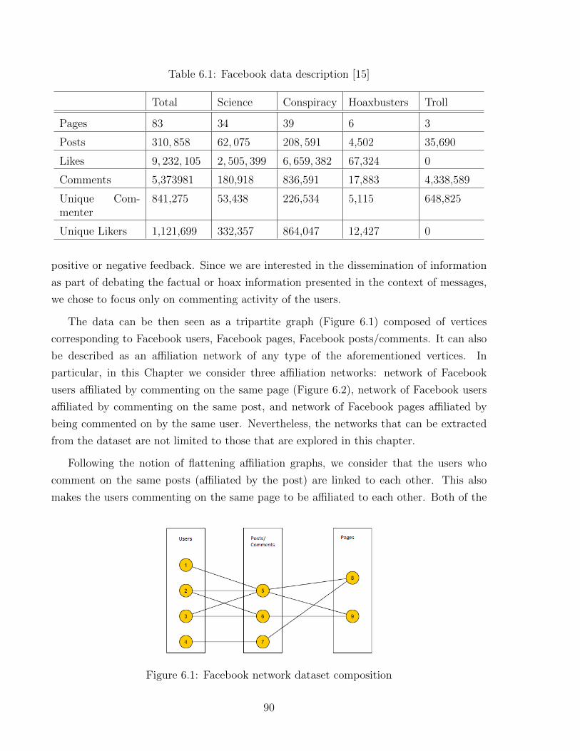
In Chapter 6 we consider Facebook data of over 800 thousand users and their com-
menting activity on 81 pages that have been acquired from Facebook and given to us by a
research group in IMT Institute for Advanced Studies [15, 16]. The dataset is particularly
interesting as it provides abundant of data on the distribution of legitimate (scientific) and
hoax information on Facebook. Bassi et al. [16] have already conducted multiple studies
on the dataset from the static point of view of the network. We are, instead, interested in
10
the analysis of the network from a dynamic point of view and in the observation of the evo-
lution of communities that are formed around the scientific and hoax data. Therefore, to
reach our goals, in this Chapter we concentrate on Facebook network employing temporal
betweenness and eigenvector centrality measures in order to observe the effect of time on
the importance of the various users whether being a science user or a conspiracy distributor.
We identify Facebook users who accelerate the flow of information, and become important
as the information flows in time. Similar to Chapter 5, we identify these “invisible rapids”
and “invisible brooks” by comparing our results with static betweenness measure. By em-
ploying the eigenvector analysis and comparing temporal and static results we detect a
similar behaviour: nodes that we call “shockers” and “breakers”. Shockers denote nodes
that are deemed important and influential in time, yet do not appear among static influen-
tial nodes. Breakers show the exact opposite characteristics by being statically important
and influential, but staying in the unimportant group temporally.
In Chapter 7, we concentrate on data extracted from YouTube. By using standard
techniques, we analyse rate of propagation of videos among friends and subscribers. We
also study the relationship between the popularity of a video and its propagation rate.
We, then, conclude by evaluating similarity parameters among users. This study has been
performed on ten datasets, each containing the data for around 10,000 users, collected
using a snowball sampling method. The analysis is conducted by employing classical
statistical metrics, which focus on the static representation of the network without making
any temporal assumptions. Our datasets have two separate networks for friendships and
followings (subscription), which allow us to analyse both networks in the same settings,
and at the same time. The results of this Chapter are published in the following papers:
• Amir Afrasiabi Rad and Benyoucef Morad. “Measuring propagation in online social
networks: the case of youtube”. Journal of Information Systems Applied Research,
(2012). 5(1) pp 26-35.
• Amir Afrasiabi Rad and Benyoucef Morad. “Similarity and Ties in Social Networks:
a Study of the YouTube Social Network”. Journal of Information Systems Applied
Research, (2014). 7(4) pp 14-24.
Finally, in Chapter 8 we introduce social commerce as an emerging platform in software
engineering and electronic commerce. Social commerce sparked after the creation of Web
2.0, and, consequently, emerge of social networks and all of their analysis techniques.
Therefore, social networks are considered as the backbone and enabler for social commerce.
11
As social commerce is not yet well-defined, we provide a framework for explaining it,
and to understand its ties to social networks, its processes, and its design challenges.
Our framework acts as a guideline intended for social commerce platform developers to
streamline the features and processes that should be included in their platform. The
results of this Chapter are published in the following:
• Amir Afrasiabi Rad and Benyoucef Morad. “A model for understanding social com-
merce”. Journal of Information Systems Applied Research, (2011). 4(2) pp 63-73.
12
Chapter 2
Background
In this chapter we introduce on-line social networks and we review the most common
parameters that have been used to analyse their structure, focusing especially on social
influence since it is considered as one of the main motivations for studying social networks
and social interactions. We also touch on business motivations for social network analysis
at the end of this chapter.
2.1 On-line Social Networks
Social networks, in general, are defined as a social structure containing a set of members
and a set of ties between them. The members can be human, animal, and even non-
living entities, that have a communication mechanism [116]. On-line social networks are
computerized successors of off-line social networks. They were brought to life by the birth
of Web 2.0, and can be defined as a system in which users are avatars or representative
profiles of their owners (humans or bots), and they may create explicit links to other
users or content items. On-line social networks have a huge difference from off-line social
network since the on-line versions are easily navigable and processable whereas a huge
effort is needed for performing the same operations on the off-line ones [40].
In a comprehensive study of social networks, Boyd and Ellison [40] identify three distinct
purposes for the formation of on-line social networks. First, as life becomes more and more
hectic, and humans, as well as businesses, need to communicate with disparate geographical
locations as part of the global village idea, on-line social networks are useful tools to
maintain existing social ties, or make new social connections. Therefore, on-line social
networks make it easy for their users to reach their extended networks. Meanwhile, social
13
networks act as a personal news agency for its members [73]. Being easily navigable, on-
line social networks serve as an easy to access medium to find new, interesting content
by filtering, recommending, and organizing the content uploaded by users. Later in this
thesis, we will see how similarity of on-line social friends makes it easy to access to the
content that are interesting to us, and existence of acquaintances help propagating our
interests in the on-line social network.
Even though social networks were scientifically defined in 1930s, no mathematical mod-
elling or a formal study was conducted on them until 1950s. It was then that mathemati-
cians represented the social networks, a pure sociological concept at that time, as graphs
and started developing theories on their bases. In 1980s, the social network became a
mainstream field in mathematics, statistics, psychology, etc. However, it was not until
1990s when social networks were officially introduced to the web by Classmates.com1 as
a by-product of Web 2.0. Classmates.com, although referred as the first on-line social
network, did not have full characteristics of social networks as it did not allow direct links
between its members, and members only had the choice of forming an affiliation network
between the members and the schools they attended. Two years later, SixDegrees.com2
was created as the first social network allowing the creation of links of between members.
On-line social networks, nevertheless, did not gain their popularity until early 2000s, when
a number of social networks were created and further developed.
Nowadays, there are multiple social networks, and some of them such as LinkedIn3,
Instagram4, YouTube5, etc. are dedicated to a special purposes whereas others such as
Facebook6, MySpace7, etc. are general purpose social networking sites. It should be noted
that all of them, no matter how they are used, contain the basic features of social networks
(see Section 2.1.4).
Other than their application, on-line social networks can be categorized into two large
classes of open and private networks. The posted content and profiles of members of the
open social networks are open to public, or at least to all members of the social network,
unless otherwise privatized by the owner. YouTube, and Twitter8 are examples of open
social networks. On the other end of spectrum, exist the private social networks, such
1www.classmates.com2www.sixdegrees.com, which is discontinued at present day3www.linkedin.com4www.instagram.com5www.youtube.com6www.facebook.com7www.myspace.com8www.twitter.com
14
as Facebook, PhotoCircle9, etc. In these social networks, the default setting preserves
complete or at least some privacy for the users, unless otherwise modified by the user, such
that the profiles and shared content can only be visible to the friends, and in some cases
followers10.
These categorizations, and also the sociological aspects behind the rapid growth of
social networks are still the focus on some areas of social network analysis even though
one of the main ideas explaining both concepts are user-centric nature of social networks.
Nevertheless, it is not the focus of this thesis, so interested audience are referred to [40, 23].
Before explaining different attributes of social networks, we need to have a short survey
on the definition of graph, as the underlying model to study social networks, which will be
used extensively in the rest of this thesis.
2.1.1 Graph’s Terminology
Graphs are a fundamental construct in complex SNA research, and the use of graph theo-
retic algorithms and metrics to extract useful information from a social graph is a primary
method of analysis in SNA. Formally, a social network is represented as a graph G = (V,E),
where V (G), represents the set of vertices, and E(G) refers to the set of edges in the graph
(simply V and E when no ambiguity arises) and both consist of a finite number of elements
n = |V | and m = |E|, respectively ([60]). The edges in the graph between u ∈ V and
v ∈ V is represented as a pair (u, v) ∈ E.
A graph can be directed or undirected. In a directed graph, an edge e is represented by
an ordered pair, and, if an edge (u, v) exists, u is a predecessor of v; we also say that the
vertex u dominates node v. A directed graph is called reflexive or digraph if there is no u
such that (u, u) ∈ E. Let deg(v) denote the degree of a vertex v in an undirected graph,
let outd(v) and indeg(v) respectively denote the in-degree and the out-degree of vertex v
in a directed graph. A digraph is called a tournament when there is at least one directed
link between any two different vertices. It is also called transitive if for any three vertices
u, v, z, if both (u, v), (v, z) ∈ E, then (u, z) ∈ E as well.
Let d(u, v) denote the shortest distance between vertices u and v ∈ V . The eccentricity
ε(v) of v ∈ V is defined as maxv{d(v, u) : u ∈ V }. The diameter of G corresponds to the
maximum vertex eccentricity maxv{ε(v)}.9www.photocircle.com
10Friendship represents a mutual tie between users whereas follower-ship is representative of a uni-directional tie between users
15
A graph is often represented using an adjacency matrix. An adjacency matrix A(G)
(simply A when no ambiguity arises) is an n× n Boolean matrix (with n = |V (G)|) where
entry aij = 1 if and only if (i, j) ∈ E(G); it is zero otherwise.
A walk is a sequence v0, e1, v1, ..., vk of vertices vi and edges ei such that for any i, edge
ei has endpoints v(i−1) and vi. A walk that has distinct vertices and edges is called a path.
In a cycle the start and the end points of the path are the same.
Finally, a hypergraph is a graph where multiple edges are allowed between pairs of
vertices.
Social networks are commonly represented by graphs. In the case of a social network,
the set of vertices V of its corresponding graph often represents individuals and set of edges
E may represent relationships, friendships, or sometimes communications among them.
2.1.2 Structure of Social Networks
Over the time, the mathematicians, physicists, and computer and social scientists tried to
formulate and model the structure of social networks. This evaluation has become easier
due to the availability of extensive data on social networks. The structural properties of
social networks are determining factors in influence maximization, social network catego-
rization, actor ranking models, and so on. Basically, other then techniques that focus on
text mining and Natural Language Processing (NLP), almost all other SNA models are
based on the structure of social networks.
As a general classification, we can classify social networks in two big categories: ho-
mogeneous and heterogeneous. Social networks are homogeneous, when vertices and edges
are all of the same type, or heterogeneous, when there exist more than one type of node or
edge in the graph ([81]). If we restrict the heterogeneous networks in a way that vertices
of the same type cannot have an edge between themselves, we have an affiliation network
[76]. Affiliation networks, however, can be easily converted to simple networks (homo-
geneous networks) at the price of information loss. Moreover, social networks might be
represented by hypergraphs in which hyperedges connect more than two vertices [14]. All
the above-mentioned network types can have directed or undirected edges.
In the rest of this section we discuss about structural characteristics of such networks,
focusing more on homogeneous social networks. We will see that the Facebook, YouTube,
and Knowledge-net networks studied in this thesis, while some being heterogeneous, and
other homogeneous, all fall in the categories of small world and scale-free networks.
16
Random Graphs. Random networks have been heavily studied in the past few decades.
Erdos and Reyni [42] were the first researchers who conceptualized the model for random
graphs. Their interpretation of random graphs includes a set of edges between pairs of
node with equal independent probability. The model is represented by G(n, p), where p
refers to the probability that an edge is included in the graph. Thus, all graphs with n
nodes and m edges have equal probability pm(1− p)(n2)−m.
The parameter p in this model can be thought of as a weighting function. Therefore,
when p increases from 0 to 1, the likelihood that the resulting graph become a dense
graph increases. Similar to most probabilistic models, the behaviour of random graphs
are studied for the cases where n tends to infinity. Random graphs might not have real
examples among on-line social networks, but they show very interesting characteristics in
aforementioned cases, and are basis for study of some social networks.
Small-world networks. In 1960s, Milgram [82] carried out a famous experiment in-
volving passing letters from one person to another in order to deliver each letter to its
designated destination. The experiment showed that the delivery is possible in very small
average hops of only six. This result was called the small world effect meaning that the
vertices of the graph are connected to each other by a very short path. Specifically, a small-
world network is a network where the distance d between two randomly chosen vertices
grows proportionally to the logarithm of the number of nodes n in the network (d ∝ log n)
[117]. Others define the same value d proportional to both distance and number of vertices
in the graph. For instance, Newmann [87] defines d as d−1 = 112n(n+1)
∑i≤j dij
−1, where dij
is the shortest distance between i and j. Nevertheless, the logarithmic definition is much
more popular and mathematically provable. Figure 2.1 presents the random graph along
with small-worlds.
The small-world effect implies that the spread of information in the network is fast.
The effect is also tested on real networks and it is proven that some social networks display
small world characteristics [6, 85, 86]. Bollabas and Riordan [20] later showed that some
social networks posses characteristics resembling to the power law distribution, which led
to creation of new class of social network structural models.
Scale-free Networks. in 1965, studies on the academic network of citations showed
that the citations that papers receive have a long tailed distribution following Pareto or
power law distribution [122]. This was the starting point for mathematically modelling
such networks. Barabasi [10] followed the previous studies and mapped them on the study
17
Figure 2.1: Random Graphs Vs. Small-Worlds [117]
of World Wide Web. He discovered that World Wide Web shows indications of power law
distribution. He and his colleagues called such networks, which exhibit a power-law degree
distribution, Scale-free Networks.
To explain the scale-free behaviour, Barabasi and Albert proposed a mechanism, called
preferential attachment, that explained creation process of scale-free networks [10]. Figure
2.2 represents the process of preferential attachment, where a new vertex links to other
vertices proportional to their degree. Later, it is discovered that preferential attachment
can only explain a subset of real-life scale-free networks [36]. Li et al. [77], recently, offered
a more precise model for scale-free networks called scale-free metric. Briefly, let G be a
graph with edges E, and the degree of a vertex v by deg(v). The scale-free metric SF (G)
is defined as a value that is calculated directly from the joint degree distribution of the
graph. Therefore,
SF (G) =
∑(u,v)∈E deg(u) · deg(v)∑
(u,v)∈E deg(u) · degmax(v)(2.1)
where the denominator is the maximum value in the set of all graphs with degree dis-
tribution identical to G. Scale-free measure is always between 0 and 1. If the graph is
set in a way that the high degree vertices tend to connect to other high degree vertices,
the value tends to be closer to 1, and when the high degree vertices are connected to low
degree vertices, the value becomes closer to 0. Therefore, the scale-free networks are often
described as self-similar.
18
Figure 2.2: The Emergence of a Scale-Free Network as a Result of the Preferential Attach-ment [21]
2.1.3 Social Network and Communities
Although we do not technically analyse communities in this thesis, this concept is so
important topic in SNA that needs introduction. In fact, detecting the communities is
one of the main areas of interest in structural SNA. Communities are formed from social
network users who are tightly linked together. There is ongoing research on community
detection on social networks. Fortunato [47] surveyed almost all important algorithms that
lead to detecting communities in the graphs. We, specifically, develop over community
detection models based on betweenness and modularity [87]. We will detail such models
in the next chapters.
2.1.4 Characteristics of Social Networks
Now that we have defined the most renowned social-network structural models, we provide
a brief survey of some important characteristics of social networks.
Diameter
Diameter in graphs is defined as the longest shortest path in the graph. In Social Networks,
however, researchers often refer to the diameter with different meanings. For instance,
Esley and Kleinberg [38] define the diameter as the average of shortest paths (we call this
average diameter) in the graph as opposed to the normal graph-theoretic definition that
defines the diameter as the longest shortest path.
19
As discussed in 2.1.2, social networks, characterized by small-worlds, have small diam-
eters. However, first, as initial models of social networks revolved on the random graph
structure, the probability to have social networks with small diameter was very low, but
reality proved otherwise. Secondly, not all social networks are small-worlds. The reason
why it is said that social networks have small diameters is that a wide range of social
networks have small average shortest path length, and consequently are referred to small
worlds; World Wide Web being one of the most common examples which is considered a
small world due to its small average shortest path (in case of disconnected networks, we
have several small worlds).
Why knowing the social network diameter is important? As stated, the diameter is
representative of how close (from the geodesic distance point of view) the actors are in the
network. Thus, the diameter can be used as a measure of global density of the network,
when the definition by Esley and Kleinberg [38] is used.
Navigability
As discussed in 2.1.2, Milgram’s experiment showed that most real life social networks are
in fact navigable small-worlds meaning that not only do exist short paths connecting most
pairs of people, but also each vertex can build (short) paths to any other vertex just by
using only local and some structural global knowledge. This characteristics is completely
defined, and observable in the small-world model developed by Watts et. al. [118]. Their
model is based upon multiple hierarchies defined based on the properties of the vertices
and the network structure. The model also incorporates a greedy algorithm that attempts
to get closer to the target in various dimensions at every step. Unfortunately, no attempt
has yet been made to investigate this model theoretically while many empirical analysis
has been conducted on it.
Although we do not directly investigate this model, we will see how navigability affects
influence propagation while analysing YouTube social network.
Giant Components
Although we do not refer to components in this thesis, introduction of communities is
not complete without introducing connected components in the graph. Components are
composed of a set of connected vertices that are disconnected from the rest of the graph.
These are different from communities in a sense that vertices in different communities can
still be connected to each other, but more densely connected inside the community.
20
Giant components are defined as connected components containing a large number of
vertices, often more than half of the vertices in the graph. Small-world effect implies
that that social networks must have a large connected component containing most of the
vertices. Giant components are studied in random graphs and small-worlds in different
disciplines, mathematics, computer science and physics.
Mixing
Knowing the degree distribution of social networks gives abundant information to under-
stand the network. However, degree distribution is only a local property, and does not
guide us to identifying the global structure of the network in a precise manner. Therefore,
it is very important to know if the high degree vertices are linked with other high degree
vertices, similar to what exists in scale-free networks (see 2.1.2), or they are linked with
low degree vertices or any other patterns. These link patterns are called mixing in social
networks. The mixing in social networks is studied in various attempts, and the result of
the studies exhibited a positive co-relation between the degree of node v and its neighbours
[72, 89, 90]. This mixing pattern that is common in social networks, is called assortative
mixing.
2.2 Social Influence
One of the important applications of social networks is information dissemination, and this
is not possible without social influence. Thus, social influence is an important strategy that
is embedded in the concept of social network. Merriam-Webster dictionary defines influence
as “the act or power of producing an effect without apparent exertion of force or direct
exercise of command”. In scholarly articles, social influence is defined as the phenomenon
where the actions of a user can induce his/her friends to behave in a similar way [98].
In social networks, influence is created by passing an idea to a networked friend. Social
network users pass their ideas by creating new content or reusing pre-generated content
(i.e., reposting other people’s ideas or quoting other people in interactions). It is apparent
that social influence is the result of content that is generated by social network users. In
fact, more generated content can trigger more (positive or negative) influence.
Various social factors participate in the influence, and influence occurs for a wide variety
of reasons. Flanagin and Metzger [46], for instance, provided the most comprehensive
model for user participation in social activities by surveying 684 people from different
21
demographics. Their survey revealed twelve factors that actively affect how and why
people participate in social activities (Table 2.1 shows the top seven of those factors). The
survey shows that, in addition to entertainment related reasons, most people engage in
social activities to produce ideas and gain or distribute information.
Table 2.1: Top seven reasons for social participation
Top Reasons Ranked by the General Public Top Reasons Ranked by On-line Users
1. To get information 1. To stay in touch
2. To be entertained 2. To provide others with information
3. To pass the time away when bored 3. To get information
4. To relax 4. To get to know others
5. To generate ideas 5. To be entertained
6. To learn how to do things 6. To have something to do with others
7. To learn about myself and others 7. To pass the time away when bored
In a different study, Dholakia et al. [33], categorized social participation factors into
five major categories, namely: Purposive Value, Self-Discovery, Maintaining Interpersonal
Interconnectivity, Social Enhancement, and Entertainment Value. All categories have a
direct relation with influence in social networks and virtual communities. We summarize
all factors affecting influence in Table 2.2.
Although many different models are developed for modelling influence propagation is
social networks, most of the aforementioned factors are sometimes ignored in those mod-
els, and, specially, in identification and ranking of influential actors in social networks.
The challenge causing this issue pertains to difficulties related to collection of such data.
Therefore the analysis of influence ranking is usually restricted to graph-theoretical meth-
ods called sociometric measures of social networks.
2.2.1 Sociometric Techniques for Ranking
Centrality measures are designed as indicators that identify and rank the most important
vertices and edges within a graph. The applications of the centrality measures are very
diverse ranging from identifying the influential people in social networks to predicting
patterns of disease contamination and propagation, to dividing the graphs into sub-graphs
also known as communities. However, it should be noted that centrality indices have
three important limitations. First, their application is domain dependant. Therefore, a
22
Table 2.2: Factors affecting influence
Factor Description
Connections It is generally perceived that a higher number of connections is indicativeof higher popularity, and popular people are more influential than others[113]. Moreover, when you have more connections, more people hear yourvoice, and your ideas may be distributed faster and wider. On the otherhand, you will also hear more voices; hence your ideas might becomeblended with other people’s ideas.
Networking Pur-pose
The networking purpose has a significant effect on the choice of content toconsume and generate. To identify the networking purpose, the contentof communications must be evaluated. To do so, Weng et al. [120],Romero et al. [98], and Huberman et al. [61] introduced the notion oftopic-based influence.
Demographics By evaluating the demographics of social network users, we can determinewho shares similar interests with whom [74].
Group Member-ship
Group membership provides a fast way to identify the interests of users,as users with similar interests in an issue tend to connect together in agroup.
measure that applies to a domain, and provides good results is not necessarily useful for
other domains as well. Meanwhile, the values for the centrality measures are just relevant
to the structure of the graph, and undermine the internal characteristics of the vertices
and edges. The centrality values are significantly different for high ranked vertices and
edges, but show very little variation in the rest of the graph. Therefore, the ranking of the
vertices and edges are not very useful in such cases, except the situations where the goal is
to divide the graph into communities. In community detection algorithms that work based
on centrality measures all values for centrality are important. In this thesis, we focus on
betweenness and eigenvector centrality values, yet we believe that general understanding
of centrality measures helps the reader to understand the motivation and results of the
chapters along their methodologies and content. Hence, we provide a summery of most
renowned centrality measures in Table 2.3, and discuss them in this chapter. However,
centrality measures are not limited to the measures discussed here.
Geometric Measures
Geometric measures are those measures in which the importance is a function of distances;
more precisely, a geometric centrality depends only on how many nodes exist at every
23
Table 2.3: Sociometric Techniques for SNA
Metric Description
Degree refers to the number of edges that connect the node to other nodes in thenetwork
Closeness Closeness centrality is defined over the connected graphs, and it is denotedas the average distance of a vertex from all other vertices in the graph
Eigenvector eigenvector centrality measures the prestige of a node and translates intothe phrase: a node is important if it is linked to by other important nodes.Hence, the eigenvector centrality is more meaningful than degree centrality,so that a node receiving many links does not necessarily have a high eigen-vector centrality (it might be that all linkers have low or null eigenvectorcentrality)
Katz It is very similar to eigenvector centrality with heuristic components
PageRank PageRank estimates the importance of a vertex by counting the numberand quality of links to it.
HITS very similar to PageRank. It is an iterative algorithm that computes hubscore and authority scores both at the same time. A page is authorita-tive if it is pointed by many good hubs pages which contain good list ofauthoritative pages , and a hub is good if it points to authoritative pages
SALSA an extension to HITS in order to assign high scores to hub and authorityvertices based on the quantity of edges among them
Betweenness measures the importance of a vertex based on how often the vertex happensto be located between two or more communities
ClusteringCoefficient
Clustering coefficient measures the degree to which graph vertices tend toform a cluster together
Modularity measure the strength of division of a graph into modules, also known ascommunities
distance.
— Degree centralities. Degree centrality of a node v is the simplest and historically
the first centrality measures that has been used in SNA. It is usually defined as the degree
deg(v) of node v, divided by n − 1 to restrict the metric in the [0, 1] range (figure 2.3).
Degree centrality can be interpreted as the risk of being infected in the graph or the
opportunity of infecting others. For that reason, it is one of the most-used measures in the
studies about spread of disease in communities (e.g. [22]).
Analogously, one can define the in-degree centrality indeg(v) and the out-degree cen-
24
Figure 2.3: Degree centrality of a graph: Vertices 1, 7, 11 have degree 1/12, vertices 3, 5,6, 9, 10 have degree 0.25, and the rest of vertices have degre 1/6
trality outdeg(v) of a node v in a directed graph. A high in-degree can indicate a tendency
towards being a content consumer, or it means a high risk of being infected. If a user with
a high in-degree has a low or zero out-degree value it might be an indication of inactivity.
A higher number of received messages might also indicate that there are opportunities
for the user to be influenced by his/her friends. A vertex with high out-degree has more
opportunities to influence others by its behaviour because it has more ways to transfer its
characteristics. The combination of in-degree and out-degree centrality measures helps in
detecting spammers and inactive users [4]. A user with zero (or close to zero) in-degree
and high out-degree might be a spammer.
— Closeness centrality. An important node is typically close to others in the network,
and can communicate quickly with them. The basis of the closeness centrality is quick
communication. Closeness centrality is defined over the connected graphs (its modified
version also works for disconnected graphs), and it is the average distance of a vertex from
all other vertices in the graph [100]. The metric is usually reversed in order to restrict the
closeness value in [0, 1] (figure 2.4):
CC(v) =∑u∈V
n− 1
d(v, u)(2.2)
Closeness centrality represents the amount of information that can be distributed by
a vertex in the graph if it is accepted that information travels through the shortest path
between the vertices knowing that the distance between a vertex and itself is zero. Thus,
closeness centrality is very popular in analysis that involve travel of information, goods,
25
Figure 2.4: Closeness centrality: vertex b has the highest closeness equal to 0.8, and thecloseness values are 0.5 for a, and 0.57 for the rest of vertices
vehicles, etc. Conti et al. [28], for instance analyse the disruptions in US flight networks
employing closeness centrality extensively.
However, in most cases, the distance that information travel between two vertices in
the graph is not necessarily through the shortest path between them. Thus, Newman [91]
provided an algorithm that calculates the closeness of a vertex in the graph based on a
series of random walks starting from that vertex. This measure of closeness is more realistic
to social networks involving people.
In an attempt to extend the applicability of closeness centrality to disconnected graphs,
Dangalchev [31] defined closeness as the inverse of 2 to the power of distance:
CCD(v) =
∑u∈V
2−d(v,u) (2.3)
The closeness centrality is extended to disconnected directed graphs by Boldi and Vigna
[19] as:
CCB(v) =
∑u6=v
d(v, u)−1 (2.4)
where 1/∞ = 0.
Prestige Measures
Prestige measures of prominence take into account the differences between the neighbour-
hood set, considering that their rank would affect the rank of the node. Prestige measures
better apply to directed graphs, but are still useful for undirected graphs. We specifically
focus on eigenvector centrality in this thesis, but we are compelled that introduction of the
26
measures that are very close to eigenvector centrality develops better understanding of this
metric. Thus, we briefly introduce the background and application a few of eigenvector
centrality’s siblings.
— Eigenvector centrality. Degree centrality awards the same centrality score for every
link a vertex receives, but not all vertices are equivalent. Some vertices are more relevant
or important than others. For instance, while vertices 2 and 8 in figure 2.3 have the same
degree centrality, it is clear that they should be valued differently. Vertex 8 should be
considered more important than vertex 2, since vertex 8 is connected to vertices 5 and 9
that are more important than what 2 is connected to (1 and 3). Therefore, being connected
to an important vertex, logically, affects your importance more than being connected to
a non-popular vertex. Eigenvector centrality measures the prestige of a node giving more
importance to nodes that are linked to other important nodes. Hence, the eigenvector
centrality is more meaningful than degree centrality, so that a node receiving many links
does not necessarily have a high eigenvector centrality (it might be that all linkers have
low or null eigenvector centrality). Moreover, a node with high eigenvector centrality
is not necessarily highly linked (the node might have few but important linkers) [103].
Eigenvector centrality is tied with popularity. Thus, it is very applicable in the studies
analysing and designing campaigns, whether, political [49], advertisement [104], or any
other form of campaign.
Eigenvector centrality is computed by:
CE(v) = λ−1∑u
av,uCE(u) (2.5)
where λ is a constant. However, the recursive dependency of value makes it impossible to
calculate the eigenvector centralities using Equation 2.5 in a recursive manner. The reason
for this is that the base case for the recursive function does not exist. Hence, eigenvector
centrality is redefined as the eigenvector of the adjacency matrix λx = Ax. Therefore,
we see that x is an eigenvector of the adjacency matrix with eigenvalue λ. To make sure
that the centralities are non-negative,it can be shown (using the PerronFrobenius theorem)
that λ must be the largest eigenvalue of the adjacency matrix A, and x the corresponding
eigenvector (CE(v) = xv).
Referring back to Figure 2.3, the adjacency matrix for the graph presented in the figure
is as following, which shows the eigenvector centralities for vertices 2 and 8 are 0.19 and 0.31
respectively, while 5 has the highest eigenvector centrality of 0.44. This shows the purpose
27
of eigenvector centrality that differentiates the nodes based on who they are connected to.
We discuss about this measure more in this thesis.
x = 0.08 0.19 0.39 0.32 0.44 0.37 0.15 0.31 0.31 0.24 0.10 0.20 0.18
( )1 2 3 4 5 6 7 8 9 10 11 12 13
— Katz’s index. Katz centrality was introduced by Leo Katz and is used to measure
the degree of influence of an actor in a social network [65]. Katz centrality is normally
used in directed networks where measures like eigenvector centrality are rendered useless.
Unlike typical centrality measures which consider only the shortest path between a pair
of vertices, Katz centrality takes into account the total number of walks between a pair
of vertices. Hence, Katz centrality puts a step forward and includes more nodes than the
direct neighbours, like eigenvector centrality while penalizing the distant connections by a
attenuation factor α in (0, 1). Thus,
CK(v) =∞∑k=0
∑u
αk(Ak)vu (2.6)
Katz’ measure might be used interchangeably with eigenvector centrality, but in di-
rected graphs, it yields extreme usefulness. Due to the fact that this measure can be ap-
plied on directed graphs, it is mostly used for direct influence models, such as behavioural
modelling of networks, and analysis of influence sources in the network. An example of
such studies is Mizruchi’s study of behavioural cohesion and similarity in networks [84].
— PageRank Centrality. PageRank is one of the most discussed and quoted prestige
indices in use today, mainly because of its alleged use in Google’s ranking algorithm.
PageRank estimates the importance of a vertex by counting the number and quality of
links to it. It is generally assumed that the more popular the vertex is, the more links
it receives from other vertices [93]. By definition, PageRank of set of web pages is an
assignment CR satisfying:
CR(v) = β∑u∈P (v)
CR(u)
outdeg(u)+ βr(v) (2.7)
28
such that β is maximized and L1-norm of R is equal to one. In the aforementioned equation,
r is some vector over the web pages that corresponds to a source of rank, and P (v) is the
set of web pages that v points to.
— HITS. Hyperlink-Induced Topic Search (HITS; also known as hubs and authorities)
is a graph analysis algorithm, developed by Kleinberg [68]. The idea behind HITS is very
similar to that of PageRank’s, and is that a page is authoritative if it is pointed by many
good hubs - pages which contain good list of authoritative pages -, and a hub is good if
it points to authoritative pages. Therefore, HITS algorithm is an iterative algorithm that
computes hub score h(v) and authority scores a(v) both at the same time.
h(i+ 1) = a(i)AT
a(i+ 1) = h(i+ 1)A(2.8)
If done for infinite iterations, this process converges to the left dominant eigenvector
of the matrix ATA. This value refers the authority score of vertices of the graph, the hub
values can be easily computed based on authority scores (the left dominant eigenvector
of AAT ). Therefore, it is obvious that both vectors are left and right singular vectors
associated with the dominant singular value in the singular-value decomposition of A [43].
— SALSA. Stochastic Approach for Link-Structure Analysis (SALSA) is a graph mea-
sure designed by Lempel and Moran [75] as an extension to HITS in order to assign high
scores to hub and authority vertices based on the quantity of edges among them. SALSA
extends HITS by applying it on L1-normalized adjacency matrix of A. Therefore,
h(i+ 1) = a(i) AT
a(i+ 1) = h(i+ 1) A(2.9)
This normalization causes simplification in the process of computation of SALSA, as it
does not need the iterative process required for HITS. In this process, we initially compute
the connected components of the symmetric graph induced by the matrix ATA. In this
graph, based on the matrix ATA, two vertices are connected if they had common prede-
cessors in the original graphs. Then, the SALSA scores a vertex by computing the ratio
between the size of the component that the vertex belong to it and |V | multiplied by the
29
ratio between vertex’s in-degree and the sum of the in-degrees of all vertices in the same
component. Therefore, as opposed to HITS, which is an iterative algorithm, SALSA only
needs in-degrees, so only one iteration on the graph would suffice for its computation.
Path-based Measures
Path-based measures work utilizing the graph feature called shortest path(s) that pass
through a vertex in the graph. These measures mainly count the paths and manipulate
the vertex scores based on the results of counting. A great portion of this thesis is focused
on the measures discussed under this category.
— Betweenness. Betweenness centrality was first introduced by Freeman [50]. Be-
tweenness measures the importance of a vertex based on how often the vertex happens to
be located between two or more communities. The measurement method, however, only
counts the number of shortest paths that cross the vertex. If we represent the number of
shortest paths that flow between vertices x and y by σxy, and the number of those paths
that cross v by σxy(v), we can define the betweenness of v by:
CB(v) =∑u,w 6=v,σuw 6=0
σuw(v)
σuw(2.10)
The intuition behind betweenness is that if a large fraction of shortest paths passes
through v, then v is an important vertex that works as a connection point of communities
in the graph. Therefore, it is clear that eliminating such vertex from the graph would
disrupt the communication between different parts of the graph, and create separate com-
munities. Therefore, betweenness centrality concerns about the information flow, rather
than structural positioning of the vertex in the graph, the feature that is the basis for
prestige measures. Figure 2.5 expands on this difference in an example.
A few years later, Freeman et al. [51] suggested that not all communications between
graph entities go through shortest paths, and in fact messages may choose any path for
transmission. In fact, if we take the graph as the set of rivers starting at s and ending
at t, each river can only carry a maximum flow of water without flooding. Hence, they
developed the flow betweenness concept based on the idea of the maximum flow. The flow
betweenness of the vertex v is defined as the maximum flow that can be carried out from
s to t passing through v, averaged over all s and t in the graph. Hence, the if gst is the
30
Figure 2.5: Betweenness centrality: vertex b has the highest betweenness as it falls into thepath for most interactions between other vertices. However, its structural measures suchas degree (3) and eigenvector (0.77) are not very high. The highest degree and eigenvectorvalues correspond to vertex f .
number of paths linking points s and t in a graph, and gst(v) is the number of such paths
that contain point v, then:
CB(v) =n∑s<t
n∑s<t
gst(v)
gst(2.11)
Newman [91], nevertheless, suggested that not all communications between graph en-
tities go through all paths, and in fact communications choose a random path for trans-
mission. Considering that, and the conditional probability characteristics, the probability
of choosing a shorter paths is higher than a longer paths. Newmann denoted these shorter
paths as geodesics, a term that we use to refer to this kind of paths in his thesis. Hence,
he argued that flow betweenness, like shortest path betweenness, can give counter-intuitive
results, and proposed a random walk version of the metric. Random walk betweenness is
calculated based on the concept of current flow analogy. Newmann’s algorithm provides a
more intuitive model for information flow, thus betweenness. Considering the networks in
Figure 2.6, the drawbacks of flow betweenness, and the random walk treatment that fixes
it are depicted.
Community-based measures
Community-based measures either use communities in the calculation, or are inspired by
formation of communities. These metrics heavily depend on the structure of the graph, and
make no assumption on the information flow in the graph or geometric characteristics of
the graph. Out of these two measures, modularity is used in the computations for Chapter
5.
31
Figure 2.6: Flow betweenness, while claiming that it passes through all the paths, itgives low betweennss value for vertex c. Random walk betweenness solves this issue, byconsidering a probability for each vertex corresponding to the paths that pass through it.[91]
Figure 2.7: Global clustering coefficient is 0.33 as a third of the triplets are closed ({c, d, e}is the only closed triplet). From a local point of view, the highest clustering coefficientbelongs to d and e, while, for instance, c has the value 1/12.
— Clustering coefficient. Clustering coefficient measures the degree to which graph
vertices tend to form a cluster together. Evidently, in social network graphs, vertices tend
to create tightly knit clusters or cliques. Interestingly, this likelihood is even more than
the chance of creation of an edge between two vertices [117]. Clustering coefficient can be
measured locally and globally. The global view gives an overall indication of the clustering
in the network, whereas local view only gives the results on how embedded a vertex is in
the graph.
The clustering coefficient is based on counting the number of triplets (sometimes called
strong ties) that are formed in the graph. A triplet consists of three vertices that are
linked together, and a closed triplet is denoted to a subgraph of three vertices that form a
complete graph K3 [79] (Figure 2.7). The global view is computed by:
CClg =number of closed triplets
number of connected triplets of vertices(2.12)
The local clustering coefficient, however, focuses on one vertex in the graph, and quan-
tifies how close the vertex’s neighbours are to forming a clique. The local clustering coef-
32
ficient for a vertex is computed by taking the ratio of edges between the vertices that fall
into the group of its neighbours divided by the number of edges that they could have if
the graph was a complete graph. Thus, if we denote neighbours of v (i.e. |N(v)|) by nv,
we will have the following equation for computing the local clustering coefficient for the
vertex v:
CCll(v) =|{(u,w) : u,w ∈ N(v), (u,w) ∈ E}|
nv(nv − 1)(2.13)
In case of undirected graphs, the number of edges in the complete graph of neighbours
would be divided by 2 resulting the whole equation be multiplied by 2. Watts and Strogatz
[117] developed a new interpretation of global clustering coefficient based on local clustering
coefficients to explain small-world phenomenon. Their model weights low degree vertices
more than high degree vertices:
CCl =1
n
n∑v=1
CCll(v) (2.14)
— Modularity. Modularity measures how modular the structure of the graph is. It
measures the strength of division of a graph into modules, also known as communities.
Modularity is mainly used as a quality metric for identifying how good the graph is di-
vided into different communities. High values of modularity shows dense communities and
sparse intra community edges, whereas low modularity is representative of non-significant
separation between communities. The intuition behind this measure is that vertices inside
a community tend to have lots of edges between other vertices in the same community
and lower number of edges with other vertices that do not belong to the same community.
Thus, modularity is defined as the fraction of edges that fall within a group minus the
expected number of edges within that for a random graph with the same degree distribu-
tion (some even consider complete graphs) [88]. Thus, supposing that sv and sw represent
the communities that v and w belong to, and svsw = 1 if v and w belong to the same
community and −1 otherwise, the modularity for two communities is defined as:
Q =1
2m
∑vu
[Avu −
deg(v) deg(u)
2m
]svsu + 1
2(2.15)
Modularity is later generalized to cover multiple communities [27].
33
2.3 Conclusion
In this chapter, we introduced the essential concepts discussed in the thesis, while provid-
ing definitions for various terminologies used throughout the thesis. The chapter mainly
focused on the static graphs. In the next chapter, we shift our focus to dynamic networks.
34
Chapter 3
Time-Varying Graphs and Temporal
Metrics
In this Chapter we introduce the notion of time-varying graph, a formal model that has
been recently proposed to describe dynamic networks encompassing different contexts into
a unique framework (e.g., vehicular, ad-hoc, satellite networks, social networks, robotic,
military networks, etc.). We also describe several temporal measures, whose corresponding
“static” version has been employed to analyse social networks.
3.1 Time Varying Graphs
Similarly to the static graphs that are defined in 2.1, TVGs are also formed from vertices
V and edges E. Nevertheless, since they address dynamical systems, the relations between
the edges take place over a time span T ⊆ T called lifetime of the system. T is the
temporal domain of the system and is equivalent to N for discrete-time systems and R+
for continues-time systems. The existence of edges should also be defined in a TVG. The
presence function, ρ : E × T → {0, 1}, indicates whether an edge exists at a given time
t ∈ T . Meanwhile, since the traversal time on every edge might be different from other
edges, the latency function, ζ : E × T → T, depicts the time that takes to traverse the
edge from its source to its target at a given time. Therefore, TVGs are described by
G = (V,E, T , ρ, ζ). The model may, of course, be extended by defining the vertex presence
function (ψ : V × T → {0, 1}), and vertex latency function (φ : V × T → {0, 1}).
Obviously, the definition of TVG imposes no restrictions on the edges or nodes. In
particular, if the presence function is always equal to one and latency is equal to zero,
35
Figure 3.1: TVG visualization by Casteigts et al. [25]
the TVG is equivalent to a static graph. There might be limited restrictions applied, for
instance, the latency function can be defined to be constant over time (ζ : E → T), over
the edges (ζ : T → T), over both (ζ ∈ T), or simply ignored. At the same time, there
might be two edges connecting two vertices starting and ending at the same time, i.e.
ρ(e1, t) = ρ(e2, t), but having different latencies, i.e. ζ(e1) 6= ζ(e2). In the latter case, the
TVG contains parallel edges and it describes a multigraph [58]. Therefore, a TVG can be
seen as a general case that covers a broad range of graphs, and this illustrates the spectrum
of models over which the TVG formalism can stretch.
Several analytical works on dynamic networks ignore ζ, or assume a discrete-time sce-
nario implicitly corresponding every time step to a constant ζ. Also, in some research
settings that are delay-free, this factor is automatically equals to zero. Such researches
include SNA even though in real-life examples it is impossible to reduce ζ to a value equal
to zero, and have null latency. In the rest of this thesis, we assume that all components of
TVGs exist unless explicitly indicated.
An example of TVG is shown in Figure 3.1. The labels on the edges represent the time
intervals when the edge exists. Note that the same labelling could be used for vertices as
well.
3.2 Temporal Concepts
In this section we introduce a number of dynamic network concepts from the TVG frame-
work point of view. We limit our review to the major concepts that frequently appear in
various fields and and abundantly referred to in the literature.
36
3.2.1 The Underlying Graph
The underlying graph U = (V,E) of a TVG G is a static interpretation of G. U flattens the
time dimension of in G and assumes an edge between two vertices if there exists at least one
edge between them in at least one instance of time. Thus, U is, sometimes, referred to as
footprint of G. While U is a helpful concept for some applications, it, unfortunately, does
not reveal any information about the structure of its corresponding TVG. For instance,
from the point of view of the simplest structural concept, connectedness, the footprint
graph and TVG do not necessarily have any correlation. Therefore, the connectedness
of U does not imply the connectedness of G over time. In a broader view, the degree
distribution of such graphs can be totally different, too.
3.2.2 Points of View
Depending on the problem setting, TVGs can be viewed from different point of views.
TVGs can generally be viewed from three different point of views. We can look at the
evolution of the system from the point of view of a given edge (edge-centric point of view),
or of a given vertex (vertex-centric point of view), or look at the global system (graph-
centric point of view) [25].
The edge-centric view revolves around indicating the existence and latency of edges
over time. The available times of an edge e is defined as the union of all times when the
edge is available, i.e. I(e) = {t ∈ T : ρ(e, t) = 1}. I(e) can also be represented by a set
of pairs of times t where ti < ti+1 as I(e) = {[t1, t2) ∪ [t3, t4), ...}, where the set of the
first items in the pairs are appearance sequence App(e), (e.g. t1, t3, ...), and the set of the
second items of the pairs are disappearance sequence Dis(e), (e.g. t2, t4, ...). Therefore,
the notation ρ[t,t′)(e) = 1 indicates that ∀t′′ ∈ [t, t′), ρ(e, t′′) = 1. The union of App(e) and
Dis(e) are referred to as characteristic times of e, and represented by ST (e).
The vertex-centric view, however, has a completely different formalism, and focuses on
the successive changes that happen in the neighbourhood of a vertex [92]. The sequence
of neighbourhood representation Nt1(v), Nt2(v), ... is useful as it can lead us to define the
temporal degree of a node. The temporal degree of v can be defined in a punctual format
as degt(v) = |Et(v)|, and its integral corresponding degree is defined as DegT (v) = | ∪Et(u) : t ∈ T |.
In TVGs, each topological event can be viewed as the transformation from one static
state to another. Hence, the evolution of the system can also be depicted as a sequence of
37
snapshots taken at different points of times as static graphs. Indeed, this is the view on
which the definition of evolving graphs is based [45]. This implies that this point of view
can be described based on characteristic times of the edges, and subsequently characteristic
times of the graph ST (G) = sort(∪{ST (e) : e ∈ E}). Thus, the sequence of static snapshots
of the graph SG = G1, G2, ..., where Gi corresponds to the static snapshot of G at time
ti ∈ ST (G), describes the graph-centric view of the TVG. Therefore, in a discrete model,
a snapshot corresponds to each new appearance of set of edges. When we talk about
snapshots in this thesis, we refer to this discrete model unless otherwise stated. It is
important to mention that in a continuous time model Gi 6= Gi+1 always holds, and in a
discrete time model, where t = i, it is possible to have Gi = Gi+1.
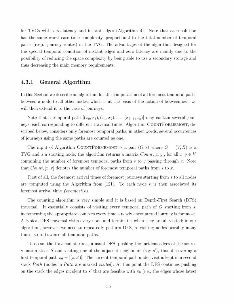
3.2.3 Journeys
Let us consider TVGs with non zero latency; i.e., ζ(e) 6= 0, ∀e ∈ E.
In G, a journey J , in its simplest form, is a temporal walk (vertices can appear multiple
times in a journey as long as the appearance occur at different times), and defined as a
sequence of ordered pairs {(e1, t1), (e2, t2),...,(ek, tk)}, such that {e1, e2, ..., ek}, called the
journey route and represented by R, is a walk in G, if and only if ρ(ei, ti) = 1 and
ti+1 ≥ ti + ζ(ei, ti) for all i < k. Of course, one may assume more restrictions and
conditions for a journey based on the application. Every journey has a departure(J ) and
an arrival(J ) that refer to journey’s starting time t1 and its last time tk + ζ(ek, tk).
The set of all journeys in a TVG is denoted by J ∗G , and J ∗(u, v) ⊆ J ∗G represents
journeys starting from u and arriving at v. A journey from u to v can also be defined in
terms of its route. Since a journey should have a temporal route, we define σ as the set
of points of times indicating when each edge of route from u to v (i.e. R(u, v)) is to be
traversed. Hence, a journey is defined in terms of R and σ as J (u, v, σ) = {R(u, v), σ}. ucan reach v (i.e. u v) if and only if J ∗(u,v) 6= ∅. It is worth mentioning that the existence
of journeys are not symmetrical and u v 6⇔ v u. The horizon of u is also defined as
the set {v ∈ V : u v}. A journey is direct if there is no delay on any of the vertices that
lie on its route from u to v. Otherwise, the journey is indirect and it waits at at least one
vertex.
Since journeys are naturally walks over time, their length can be measured from both
points of view of time and hop. Before defining the journey lengths, we need to define
a few concepts. The hop-count, |J (u, v, σ)|h = |Ri| = k, is the number of edges that
the journey traverses. The end-to-end duration of the journey is called the journey time,
38
Figure 3.2: If we suppose that ζ(a, c) = 3 and 1 for other edges, we canobserve all the journeys in this figure. While Jd(a, c) = {(a, c)}, its fore-most journey arriving at time 2 is Ja(a, c) = {(a, d), (d, c)}. Its fastest jour-ney, however, corresponds to Jl(a, c) = {{(a, b), (b, c)}, {(a, d), (d, c)}}. At thesame time, if we suppose that the latency of all edges, including ζ(a, c) are equalto 1, the foremost journey between a and e arriving at time 6 is Ja(a, e) ={{(a, d), (d, c), (c, e)}, {(a, d), (d, c), (c, a), (a, c), (c, e)}, {(a, c), (c, e)}, {(a, b), (b, c), (c, e)},{(a, b), (b, c), (c, d), (d, c), (c, e)}}. While the fastet and shortest journeys coincide atJd(a, e) = Jl(a, e) = {{(a, c), (c, e)}.
|(u, v, σ)|t or t(J ), and is simply calculated by arrival(J ) − departure(J ). The arrival
time which is defined as |J (u, v, σ)|a = σ(ek) + ζ(ek) is equal to arrival(J ). The latter is
simply referred to as a(J ). The journey length, therefore, computed based on the number
of hops is called the topological length or shortest distance, d(u, v) = min{|J (u, v, σ)|h},whereas the temporal length is two-fold by itself. The end-to-end duration of the journey
is called the delay l(u, v), and is simply equal to min{|J (u, v, σ)|t}. The second temporal
distance is called earliest arrival time, which is defined as a(u, v) = min|J (u, v, σ)|a.
Journeys are divided into three classes based on their variations based on the temporal
and topological distance [121]. Journeys with the smallest topological distance are referred
as shortest journeys Jd(u, v), the smallest delay defines the fastest journeys Jl(u, v), and
the journeys that have smallest arrival time are denoted with foremost journeys Ja(u, v)
(Figure 3.2).
A trail L is a journey in which the edges can only appear once. Trails also has variants
as shortest Ld(u, v), foremost La(u, v), and fastest Ll(u, v).
Finally, a temporal path P is a trail in which the vertices can only appear once. Similar
to journeys and trails, temporal paths have variants as shortest Pd(u, v), foremost Pa(u, v),
and fastest Pl(u, v).
Let us now consider TVGs where the latency is zero; i.e., ζ(e) = 0,∀e ∈ E. In this
39
case the notion of journey is analogous but has to be redefined by not allowing loops that
could give rise to infinite journeys. For instance in Figure 3.2, the journey cannot go back
and forth on one edge (e.g. (a, c)) in the same instance of time (e.g. time 4).
3.2.4 Connectivity
In terms of journeys, TVGs show different behaviour depending on their connectedness.
Hence, before exploring the temporal metrics of TVGs, we define concept of connectedness
in TVGs.
Definition Connectivity over time (∀u, v ∈ V, u v). A TVG is connected over time if
there exist at least a temporal journey from u to v; in other words, every node can reach
all other nodes.
Definition Round connectivity (∀u, v ∈ V, ∃J1 ∈ J ∗(u,v),∃J2 ∈ J ∗(v,u) : arrival(J1) ≤departure(J2)). A TVG is round connected if it is connected over time and for a temporal
journey from u to v, there exists a temporal journey back from v to u after the arrival the
first journey from u to v.
Definition Recurrent Connectivity (∀u, v ∈ V, ∀t ∈ T ,∃J ∈ J ∗(u,v) : departure(J ) > t).
A TVG is recurrent connected if at any point t in time, the temporal subgraph G[t,+∞)
remains connected over time.
Definition Always Connectivity (∀t ∈ T ,∀u, v ∈ V if ψ(v, t) = ψ(u, t) = 1, ∃J ∈ J ∗(u,v) :
departure(J ) = arrival(J ) = t). A TVG is always connected if it is connected over time,,
and at any point t in time, the temporal subgraph Gt remains connected for the vertices
that exist in that subgraph (vertices that are active in that subgraph).
3.3 Temporal Metrics
Most classical metrics used to analyse social networks have a temporal analogous metric
when translating the basic concepts of path, walk, degree, diameter, etc. into their temporal
counterpart. The rest of this section explores such metrics from the temporal point of view.
The summary of some of the metrics can be found in Table 3.1.
40
Table 3.1: Static and Temporal Measures
Concept/Metric Static Temporal
Eccentricity ε(v): using d(x, y)
εd(v): using hops
εl(v): using delay
εa(v): using earliest arrival
Degree deg(v) ˆdeg(v, t)
Closeness CC(v): using d(x, y)
CCd(v): temporal using d(v, u)
CCl(v): fastness using l(v, u)
CCa(v): earliness using a(v, u)
Betweenness CB(v): using d(x, y)
CBd(v): temporal using d(v, u)
CBl(v): fastness using l(v, u)
CBa(v): earliness using a(v, u)
Clustering Coefficient CCll(v) CCl(v)
Modularity Q Q
Eigenvector CE(v)ADI∗: CE1
(v)
SDI∗: CE2(v)
* These metrics will be defined in Chapter 4.
3.3.1 Degree
In a TVG G the degree of a node v at time t is indicated by ˆdeg(v, t). It is easy to see
that the definition below is a generalization of the degree in static graphs. If we sum
the temporal degrees of all nodes in the TVG, at all time snapshots, the result will be
equal to twice the number of edges times the number of snapshots that they appear in, i.e.
2 × |E(G) × T (G)| =∑
v∈V (G)
∑t∈T
ˆdeg(v, t). Therefore, if |T | is equal to 1 (i.e. there is
only one snapshot), the temporal degree coincides with the static degree of the graph.
We define max( ˆdeg(v, t)) over all t as the indicator degree of v, and∑
tˆdeg(v, t) as the
aggregated degree of v. For instance, in Figure 3.2, the indicator degree of a is 2 as there
is no instance of time when a has three incident edges. Its aggregated degree, however,
is 3. We will use the temporal degree of a graph specifically its aggregated degree in the
definition of temporal eigenvector centrality measure.
41
3.3.2 Eccentricity and Diameter
Temporal Eccentricity is defined by considering reachability through journeys instead of
paths. Let εd(u) gives the maximum number of hops required to get from u to any other
node in G. Meanwhile, εl(u) is the maximum delay that takes to get to any node starting
u. Considering the arrival times, εa(u) is denoted to the maximum of arrival time to any
node starting from u.
The graph diameter, also, has a transformed definition when defined for TVGs. The
diameter is defined as the maximum of all eccentricities over the whole graph. Thus, in
a TVG, diameter can have three forms, namely, hop diameter, referring to the maximum
eccentricity, time diameter (system-lag), denoting the maximum time eccentricity, and
rapidity, translated as the maximum of all earliest arrival times in the system. Taking the
graph in Figure 3.2 as an example, the hop diameter of the graph is equal to 2, while its
system-lag and rapidity are 4 (a e) and 8 (e a) respectively.
3.3.3 Closeness
Similarly to the case of static graphs, closeness centrality is defined over the graphs con-
nected over time, and it is the inverse of the average temporal distance of a vertex from all
other vertices in the graph [100]. In terms of distance, we define three types of closeness
in TVGs. The common closeness concerns with the average shortest hop distance between
nodes, and defined as [101, 66]:
CCd(v) =
∑u∈V
n− 1
d(v, u)(3.1)
The notion of Equation 3.1 has also been referred to as efficiency by Tang et al. [109],
who has instead defined closeness as follows:
CCd(v) = 1−
(1
W (n− 1)
∑u6=v∈V
d(v, u)
)(3.2)
where W is the number of intervals in TVG. As W = (tmax−tmin)ws
, and ws is the size of
each interval. Normalizing the whole model by W , shows that the authors assume that all
intervals have the same size ws. This restricts the application of this method to dynamic
graphs of constant interval size. Nevertheless, the factor computed by Equation 3.2 is more
similar to computing the farness than closeness.
42
Figure 3.3: Temporal Closeness: in the connected TVG over time ζ(c, d) = 2, and 1 forother edges, hence γ = 1, we have CCd
(a) = 0.87, CCl(a) = 1.83, and CCa
(a) = 1.11.
We define the variation of closeness based on the fastest journeys as fastness, which
refers to the average time that it takes to travel to all vertices. In contrast to the shortest
journeys, fastest journeys can have minimum of zero delay. Therefore, as 1/0 is undefined,
we add a constant factor γ to the denominator to avoid such situations.Note that γ does
not affect the ranking of the nodes as it is applied to closeness values corresponding to all
vertices. However, for the networks that do not have zero latency on any of the edges, γ is
equal to zero.
CCl(v) =
∑u∈V
1
l(v, u) + γ(3.3)
We define a similar metric based on the average arrival times as earliness, as the average
earliest arrival times to the vertices in the graph. This metric can also be an indicator for
reachability in time for the TVG. The aforementioned measures can be easily normalized
in [0, 1], which we skip due to simplicity. Figure 3.3 provides an example for temporal
closeness.
CCa(v) =
∑u∈V
1
a(v, u) + γ(3.4)
3.3.4 Temporal Katz Score
Calculation of Katz centrality measure in a static setting is defined in Section 2.2.1. Re-
cently, a few efforts have been dedicated to calculate the Katz centrality for the evolving
graphs, and the TVGs. Among those, Grindrod et al. [57] developed a model for comput-
ing Katz centrality along with their research on communicability of evolving graphs. We
explain their model rather in details as Katz score is a similar measure to eigenvector cen-
43
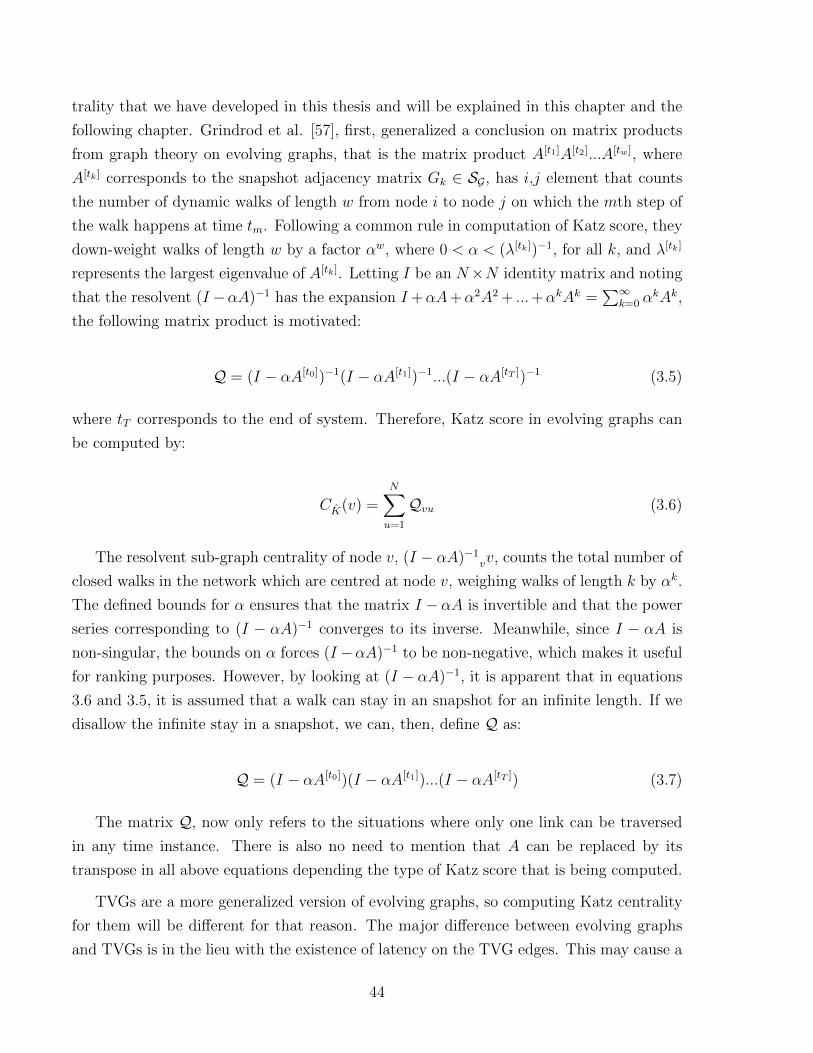
trality that we have developed in this thesis and will be explained in this chapter and the
following chapter. Grindrod et al. [57], first, generalized a conclusion on matrix products
from graph theory on evolving graphs, that is the matrix product A[t1]A[t2]...A[tw], where
A[tk] corresponds to the snapshot adjacency matrix Gk ∈ SG, has i,j element that counts
the number of dynamic walks of length w from node i to node j on which the mth step of
the walk happens at time tm. Following a common rule in computation of Katz score, they
down-weight walks of length w by a factor αw, where 0 < α < (λ[tk])−1, for all k, and λ[tk]
represents the largest eigenvalue of A[tk]. Letting I be an N×N identity matrix and noting
that the resolvent (I −αA)−1 has the expansion I +αA+α2A2 + ...+αkAk =∑∞
k=0 αkAk,
the following matrix product is motivated:
Q = (I − αA[t0])−1(I − αA[t1])−1...(I − αA[tT ])−1 (3.5)
where tT corresponds to the end of system. Therefore, Katz score in evolving graphs can
be computed by:
CK(v) =N∑u=1
Qvu (3.6)
The resolvent sub-graph centrality of node v, (I − αA)−1vv, counts the total number of
closed walks in the network which are centred at node v, weighing walks of length k by αk.
The defined bounds for α ensures that the matrix I − αA is invertible and that the power
series corresponding to (I − αA)−1 converges to its inverse. Meanwhile, since I − αA is
non-singular, the bounds on α forces (I −αA)−1 to be non-negative, which makes it useful
for ranking purposes. However, by looking at (I − αA)−1, it is apparent that in equations
3.6 and 3.5, it is assumed that a walk can stay in an snapshot for an infinite length. If we
disallow the infinite stay in a snapshot, we can, then, define Q as:
Q = (I − αA[t0])(I − αA[t1])...(I − αA[tT ]) (3.7)
The matrix Q, now only refers to the situations where only one link can be traversed
in any time instance. There is also no need to mention that A can be replaced by its
transpose in all above equations depending the type of Katz score that is being computed.
TVGs are a more generalized version of evolving graphs, so computing Katz centrality
for them will be different for that reason. The major difference between evolving graphs
and TVGs is in the lieu with the existence of latency on the TVG edges. This may cause a
44
Figure 3.4: A TVG in which the edges and vertices exist all the time with (Case I):ζ(a, b) = 2, and 1 for all other edges; and (case II) ζ(a, b) = 2, ζ(a, d) = 0, and 1 for allother edges.
link to expand in two or more time snapshots. For instance in Figure 3.4, case I, any walk
moving on (a, b) will expand in two time intervals. Plus, in TVGs, the maximum length of
a walk is equal to the lifetime of the system |T |, so iterating the walk computation until
infinite walks makes no sense unless there is an edge with zero latency on the graph (Figure
3.4, case II). We do not rule out such possibilities and design e general model that can
be applicable to all the situations. There is till one condition that the granularity of time
should be small enough so that all the edges land to their destination at the beginning of an
(future) interval, and no edge can arrive to a destination at the middle of an interval. For
instance, in Figure 3.4, the granularity of intervals can be equal to 1, 0.5, 0.25, ..., preferably
1, and any interval length of bigger that 1 is not allowed, as it guarantees that (a, c), for
instance, lands to c shorter than the end of interval. Note that edges with zero latency
always arrive to their destination at the beginning of an interval.
Therefore, using Equation 3.7 is not possible for a TVG. The reason is that there is
no way to construct a normal adjacency matrix A that represents a time snapshot, but
its edges start at the beginning of the snapshot and end at the beginning of the next
snapshot. Thus, we need to define a new concept for representing such matrices. The
adjacency matrix is inspired by the work of Wehmuth et al. [119], especially the TME
model. Our model, however, includes the zero latency edges in the TME model. We first
explain the notion of TME representation and then generalize it to our purpose.
Wehmuth et al. [119] prove that for any TVG G, there is an isomorphic directed
graph H with N × |T | vertices for which there is an order preserving bijective function
f : (V × T )(G) → V (H), such that any temporal edge e = (v, u) ∈ E(G), ρ(e, [ti, tj)) = 1
exists if and only if the edge (f(v, ti), f(u, tj)) ∈ E(H) exists. Therefore, any TVG can
be represented by a directed isomorphic graph. Based on that isomorphism, the TVG can
45
be represented by an adjacency matrix representing graph H. This matrix has N × |T |columns and rows, and non-zero entries of the matrix correspond to the temporal edges
in the matrix. Wehmuth et al. [119] call this representation as the TME model. For our
computational purposes, we fix the granularity of time as explained earlier in this section
so each edge lands at the exact starting point of any future or current time interval. We
allow landing at the start of the current time interval to make the existence of zero latency
edges possible. Let us see an example of TVG adjacency matrix corresponding to Figure
3.4, Case II.
A =
0 0 0 1 1 0 1 0 1 1 0 0
0 0 0 0 0 1 1 0 0 1 0 0
0 0 0 0 1 1 1 0 0 0 1 0
1 0 0 0 0 0 0 1 0 0 0 1
0 0 0 0 0 0 0 1 1 0 1 0
0 0 0 0 0 0 0 0 0 1 1 0
0 0 0 0 0 0 0 0 1 1 1 0
0 0 0 0 1 0 0 0 0 0 0 1
0 0 0 0 0 0 0 0 0 0 0 1
0 0 0 0 0 0 0 0 0 0 0 0
0 0 0 0 0 0 0 0 0 0 0 0
0 0 0 0 0 0 0 0 1 0 0 0
a0 b0 c0 d0 a1 b1 c1 d1 a2 b2 c2 d2
a0
b0
c0
d0
a1
b1
c1
d1
a2
b2
c2
d2
In A, nt represents the node n at time t. As it can be seen in Figure 3.4, Case II, the
edge starting from a at time zero arrives to d at time zero, so the entry corresponding to
row a0 and column d0 will be 1. With the same mode, we can fill out A’s entries. Note
that A represents a directed graph, so the entry corresponding to Aa0b1 is not necessarily
equal to Ab1a0 , even though it happens for the edges with zero latency.
Following simple lemma from graph theory (a proof can be easily found, for example,
in [30], Theorem 2.2.1), it can be easily shown that the quantity Alij counts the number of
different walks (i 6= j) or closed walks (i = j) of length l between nodes i and j. Therefore,
for instance Ala0b1 has the number of walks of length l between a and b that started at time
0 and ended at time 1. Note that if the graph does not have any edge with zero latency,
the maximum length of the walk will be equal to |T |. Now that the number of walks can
be calculated, the temporal Katz score can be easily computed by its counterpart formula
in the static model as:
46
CK(v) =∞∑k=0
∑i∈T
∑u∈V×(T ≥i)
αk(Ak)viu (3.8)
Equation 3.8 sums all the walks starting from v at all the times arriving at different
vertices at times greater than or equal to the start of the walk since the walks cannot go
back in time.
3.3.5 Temporal Betweenness
Calculation of betweenness in static graphs is defined in Section 2.2.1. Recently, Santoro
et al. [101], have explored a few centrality measures including betweenness in temporal
graphs. They extend betweenness to time varying graphs by considering foremost, shortest
and fastest journeys instead of paths. The temporal shortest betweenness of node v is then
defined as:
CJBd(v) =
∑u6=w 6=v∈V
|Jd(u,w, v)||Jd(u,w)|
(3.9)
where |Jd(u,w)| is the number of shortest journeys between u and w in the TVG, and
|Jd(u,w, v)| is the number of shortest journeys passing through v. The fastest CJBl(v) and
foremost CJBa(v) betweenness can easily be calculated by replacing Jd in Equation 3.9 by
Jl and Ja respectively.
A different notion, also called temporal betweenness while being essentially a calculation
in static graphs, has been introduced by Tang et al. [111] . They define betweenness of a
vertex at successive intervals t. To do so, a function η(v, t, u, w) is defined so that returns
the number of shortest temporal paths from u to w in which vertex v has either received
a message at time t or is holding a message from a past time window until the next vertex
is met at some time t′ > t. Similar to all betweenness measures, the betweenness is zero if
|Jd(u,w)| = 0.
CtBd
(v) =1
(n− 1)(n− 2)
∑u∈Vu6=v
∑w∈Vw 6=uw 6=v
η(v, t, u, w)
|Jd(u,w)|(3.10)
Then, the betweenness of v over the whole T is:
47
CBd(v) =
1
W
W∑t=1
C(t×ws)+tmin
Bd(v) (3.11)
where ws is the size of each footprint’s time window (the size of each interval), and the
number of the graphs in the sequence of footprints is denoted by W = (tmax−tmin)ws
.
3.3.6 Clustering Coefficient
The clustering coefficient is used in social network analysis to characterize the network
architecture. More formally, by applying to footprints, the clustering coefficient CCl(v)
indicates how close to a clique the neighbourhood of v is; in fact, it can also be extended
to cover the snapshots by taking the proportion of edges among the neighbourhood of v
divided by the maximum number of edges that could potentially exist between them in
snapshots.
3.3.7 Modularity
The modularity, measures how the structure of a given network is modular, i.e. how it
can be decomposed into subgraphs. Moreover, it can quantify the quality of a division of
a network into subgraphs. The higher the modularity is, the denser is the internal connec-
tions between nodes within communities compared to the connections between different
communities.
Amblard et al. [7] define modularity in TVGs in the footprint of the graph. There-
fore, the modularity of a pair of nodes u and v on footprint U is defined as deg(u)×deg(v)2m
.
Modularity can easily be generalized into the snapshots of the TVG as following:
Qt =degt(u)× degt(v)
2|E|t(3.12)
3.4 Conclusion
In this Chapter we introduced the notion of time-varying graph. We also described several
temporal measures. In particular, we introduced various betweenness measures correspond-
ing to different types of journeys (foremost, fastest, and shortest) that will be heavily used
in the subsequent Chapters.
48
Chapter 4
Computation of Temporal Measures
In this Chapter we are interested in the computation of some temporal measures and, in
particular, temporal betweenness. We study properties of temporal betweenness based on
shortest and foremost journeys. While shortest temporal betweenness can be computed in
polynomial time in any TVG, we observe that the situation is radically different for foremost
betweenness, because its computation is a #P problem and thus intractable. We describe
a polynomial algorithm to compute shortest betweenness, an (exponential) algorithm to
compute foremost betweenness in general settings, and one to compute it in special TVG
classes that will be relevant in the subsequent Chapters. Finally, we conclude the Chapter
with the introduction of a new temporal metric: temporal eigenvector centrality that
generalizes the well known static metric of eigenvector centrality.
4.1 Temporal betweenness
Temporal betweenness is defined in Chapter 3. We remind that temporal shortest between-
ness of v is defined as the number of shortest journeys between u and w passing through
v over the total number of shortest journeys between u and w:
CBd(v) =
∑u6=w 6=v∈V
|Jd(u,w, v)||Jd(u,w)|
The foremost betweenness CBa(v) can easily be calculated by replacing Jd in Equation 3.9
by Ja respectively to account for foremost journeys instead of shortest.
In the following we consider TVGs whose lifetime is constituted by a finite interval
of time [ts, te]. We remind the notion of journeys between two nodes u and w defined in
49
Chapter 3. A foremost journey is a walk over time that arrives at w on the earliest possible
time by leaving u any time on or after ts; a shortest journey between u and w is a path
over time that arrives at w with the minimum number of hops leaving u any time on or
after ts. We also remind the difference between a journey and a temporal path: a temporal
path does not traverse the same node more than once, while a journey may pass more than
once thought the same node, but the traversal time at those vertices must be different.
4.2 Temporal Shortest Betweenness
As mentioned, temporal shortest betweenness is similar to the non-temporal metric and
deals with counting the shortest journeys between all pairs of the vertices in the graph.
Temporal shortest journeys differ from shortest paths in a way that a legitimate shortest
path might not be temporally feasible (i.e., it might not correspond to a journey) thus
requiring a feasibility check. The algorithm described in this section is very general, and
it counts all journeys from a node to all the others under any TVG scenario.
The Algorithm
Counting the shortest journeys in TVGs can be done using a BFS-like algorithm on the
TVG inspired by the method that is developed in [121] to construct a shortest journey
spanning tree from a source to all destinations, and using the same data structure (Figure
4.1).
We need to modify the algorithm to be able to count also the number of shortest jour-
neys through any intermediate node. To do that, instead of computing only one shortest
journey, we need to maintain all shortest journeys at different instance of time. Xuan et al.
[121] prove that the prefix property exists in shortest journeys such that if the last edge,
say (u, v), of a shortest journey between vertex s and vertex v arrives at time t, then the
prefix journey (going from s to u) is shorter than all the journeys from s to u ending before
t. This property is useful in computing, and consequently counting, shortest journeys. In
order to count the shortest journeys, we modify the algorithms defined in [121] to store
the number of shortest journeys arriving at each vertex at each step of time and record
the number of hops that they have had so far in the journey.
Algorithm 1 receives (G, s) as its input, where G is the TVG and s is the starting node
from which the journeys to all other vertices in the TVG are being counted. The results are
returned in the combination of shortestCount[v, k] and shortestIntCount[v, k] matrices,
50
Figure 4.1: The data structure to store TVGs, adopted from [121]
which record the number of shortest journeys from s to v with length k, and the number
of such journeys that pass through the nodes that fall on the path of the corresponding
journey.
The algorithm starts by adding all the possible predecessors of v into the predecessor
list. Matrix Pred[v, k] stores the predecessor of vertex v. Each predecessor falls on a
“quasi-shortest path” with length k. We call this path quasi-shortest since it does not
always store the shortest path, rather, it carries some longer paths that might contribute
to the shortest path at later hops. The arrival time to some vertex v at the current step is
stored in variable arr(v), which is recorded for future path feasibility check.
The quasi shortest paths are counted and stored in Matrix count[v, k], while the
intCount[v, k] stores the number of journeys that pass through a specific vertex on the
quasi shortest path from s to v.
Some quasi-shortest paths are, indeed, the shortest paths that are recorded in the
matrix shortestCount[v, k], and the count for their intermediate vertices are stored in the
shortestIntCount[v, k]. This is determined by checking the local array tLBD[u] that gives
for each u ∈ VG a lower bound on the departure time, meaning the earliest time that
the journey can exit u. tLBD[u] is initialized to infinity and gets updated anytime that a
51
Algorithm 1: Counting the shortest journeys
input : A TVG G, a vertex s ∈ VGoutput: shortestCount[v, k] that records the number and length of the shortest
journeys from s to all v ∈ VGbegin
Initialize tLBD[s]← 0, P red[s, 0]← (), k ← 0, arr ← (),shortestCount[{., .}]← 0, count[{., .}]← 0, intCount[{., .}]← ∅, and define forall v 6= s, tLBD[v]←∞while there is v ∈ VG such that tLBD(v) =∞ and k < n do
k ← k + 1arr ← ()for (u, v) ∈ VG do
Let t = EarliestTransmit((u, v), tLBD[u])if (t+ ζ(u, v)) ≤ tLBD[v] then
add (u, (t+ ζ(u, v))) to Pred[v, k]arr[v]← min((t+ ζ(u, v)), arr[v])
for (w, k − 1) ∈ Pred[v, k] docount[{v, k}]← count[{v, k}] + count[{w, k − 1}]for each (x, i) in intCount[{w, k − 1}] do
if x exists in intCount[{v, k}] as (x, j) thenreplace (x, j) with (x, i+ j) in intCount[{v, k}] and update thecount for (x, i+ j)
elseadd (x, i+ 1) to the end of intCount[{v, k}] and update the countfor (x, i+ 1)
for v ∈ VG doif tLBD[v] =∞ then
shortestCount[{v, k}] = count[{v, k}]update shorthestIntCount[{v, k}] with intCount[{v, k}]tLBD[v] = arr[v]
tLBD ← arr
shortest journey to a vertex is found. Thus, checking whether the value of tLBD[u] for u is
infinity or not, determines if the shortest journey for u is found earlier or not.
It should be noted that function EarliestTransmit(, ) gives, for each edge (u, v), and
each time instant t, the earliest moment after t when vertex u can transmit a message to
v. If such a moment does not exist, EarliestTransmit(, ) returns +∞.
52
–Time Complexity Algorithm 1 counts the number of shortest journeys from one node
to all the others, and also the number of such journeys that pass through each intermediate
vertex. Repeating this procedure for all starting points would provide all the necessary
information to compute temporal shortest betweenness for all nodes.
Let δ indicate the maximum number of different time intervals on an edge.
Lemma 4.2.1 The number of shortest journeys from a single source s to all the vertices
in a TVG can be computed in O(n3 log δ).
Proof Using the data structure proposed in [121], and depicted in Figure 4.1, procedure
EarliestTransmit(, ) is computed in time O(log δ) due to the fact that we can apply binary
search to find the earliest transmit time. We call procedure EarliestTransmit(, ), m times
during the execution of the algorithm for a total of O(m log δ). Meanwhile, tLBD[v],∀v ∈ VGbecomes a value smaller than infinity if and only if the graph is connected and we have
found all the shortest journeys including the longest one, which is equal to the eccentricity.
In case of a disconnected TVG, we have to iterate the while loop at most n times. The
other factor contributing to the complexity appears in the nested loop for that results
which amounts to O(n2) times.
Theorem 4.2.2 The number of shortest journeys from all vertices to all other vertices in
a TVG can be computed in O(n4 log δ).
Proof The complexity mentioned in Lemma 4.2.1 has to be multiplied by n to repeat the
process from every possible starting node.
Since the most time-consuming part of the betweenness algorithm is its path counting,
the computation of betweenness is at most in the order of its path counting algorithm.
–Space complexity. The algorithm stores five matrices in memory. The predecessor
matrix, in the worst case, for each node, needs k times the the sum of degrees in the
graph, (i.e., the the eligible predecessor nodes), that is O(km) in the worst case. However,
the highest amount of space is allocated to store intCount, which is a m × (n − 1) array
where each element points to a list of all vertices that fall on the path. In fact intCount
stores, for each predecessor (for a maximum of m), the number of at most n− 1 vertices.
If we consider that the from s there is a path to every vertex, the space complexity of the
algorithm is then O(mn2).
53
Figure 4.2: Data Structure Used for Storing the Path-counts for Intermediary VerticesintCount
–Practical considerations. Due to the sparsity of the matrix that stores the path
counts, we actually use hash-maps to reduce space and time complexity of the algorithm.
In fact, we represent matrices count[{., .}], intCount[{., .}], shortestCount[{., .}], and
shortestIntCount[{., .}] as hash-maps, with count[{., .}] and shortestCount[{., .}] receiv-
ing an integer as their value, and intCount[{., .}] receiving a list of vertex and path-count
(x, i) pair as its value. intCount[{v, k}] stores the number of paths (i) starting from s and
ending at v with length k that pass through x. Figure 4.2 provides a schematic view for
the data structure that we use. While the worst case complexity is still high, hash-maps
with a good hash function reduce the access time to the stored items, which in average
becomes O(1). In our analysis on real datasets we will make use of this data structure to
speed up the computation.
4.3 Temporal Foremost Betweenness
It is easy to see that there exist TVGs where counting all foremost journeys, journey routes,
and temporal paths between two vertices is #P-complete. Consider, for example, TVGs
where edges always exist (note that a static graph is a particular TVG) and latency is zero.
In such a case any journey, journey route, or temporal path between any pair of nodes is
a foremost journey, journey route, or temporal path respectively. Counting all of them
is then equivalent to counting all paths between them, which is a #P-complete problem
(see [115]). In general, it is then unavoidable to have exponential algorithms to compute
foremost betweenness.
In this Section we first focus on betweenness based on temporal paths (and journeys) in
the general setting (Algorithms 2 and 3). We then focus on betweenness based on journeys
54
for TVGs with zero latency and instant edges (Algorithm 4). Note that each solution
has the same worst case time complexity, proportional to the total number of temporal
paths (resp. journey routes) in the TVG. The advantages of the algorithm designed for
the special temporal condition of instant edges and zero latency are mainly due to the
possibility of reducing the space complexity by being able to use a secondary storage and
thus decreasing the main memory requirements.
4.3.1 General Algorithm
In this Section we describe an algorithm for the computation of all foremost temporal paths
between a node to all other nodes, which is at the basis of the notion of betweenness, we
will then extend it to the case of journeys.
Note that a temporal path [(x0, x1), (x1, x2), . . . , (xk−1, xk)] may contain several jour-
neys, each corresponding to different traversal times. Algorithm CountFormemost, de-
scribed below, considers only foremost temporal paths; in other words, several occurrences
of journeys using the same paths are counted as one.
The input of Algorithm CountFormemost is a pair (G, s) where G = (V,E) is a
TVG and s a starting node; the algorithm returns a matrix Counts[x, y], for all x, y ∈ Vcontaining the number of foremost temporal paths from s to y passing through x. Note
that Counts[x, x] denotes the number of foremost temporal paths from s to x.
First of all, the foremost arrival times of foremost journeys starting from s to all nodes
are computed using the Algorithm from [121]. To each node v is then associated its
foremost arrival time foremost(v).
The counting algorithm is very simple and it is based on Depth-First Search (DFS)
traversal. It essentially consists of visiting every temporal path of G starting from s,
incrementing the appropriate counters every time a newly encountered journey is foremost.
A typical DFS traversal visits every node and terminates when they are all visited; in our
algorithm, however, we need to repeatedly perform DFS, re-visiting nodes possibly many
times, so to traverse all temporal paths.
To do so, the traversal starts as a usual DFS, pushing the incident edges of the source
s onto a stack S and visiting one of the adjacent neighbours (say s′), thus discovering a
first temporal path π0 = [(s, s′)]. The current temporal path under visit is kept in a second
stack Path (nodes in Path are marked visited). At this point the DFS continues pushing
on the stack the edges incident to s′ that are feasible with π0 (i.e., the edges whose latest
55
traversal time is greater than or equal to the earliest arrival time at s′), and updating
Count[s′, s′] if π0 has a foremost arrival time at s′.
In general, as soon as a temporal path π = [(x0, x1), (x1, x2), . . . , , (xk−1, xk)] is encoun-
tered in the traversal, Count[xi, xk], i ≤ k is updated only if π is a foremost temporal path,
and, regardless of it being foremost, the traversal continues pushing on the stack the edges
incident to xk that are temporally feasible with π.
Whenever backtracking is performed, however, the already visited nodes on the back-
tracking path are remarked unvisited (and popped from Path) in such a way that they
can be revisited as part of different temporal paths, not yet explored. The pseudo-code is
described in Algorithm 2.
Algorithm 2: CountFormemost.
input : (G, s) : a TVG G = (V,E), s ∈ Voutput: Counts[x, y], ∀x, y ∈ V : number of foremost temporal path from s to
y ∈ V , passing through x ∈ Vbegin
Path.push(s), Counts[., .]← 0for all w ∈ Adj(s) do
S.push(s, w)
while S 6= ∅ do(x, y)← S.pop()while x 6= Path.top() do
Path.pop()
Let π be the temporal path corresponding to the content of PathLet tx,y be the latest possible traversing time of edge (x, y)if y 6∈ Path and tx,y ≥ arrival(π) then
Path.push(y)for each (y, w) such that w 6∈ Path and ty,w ≥ arrival(π) do
S.push(y, w)
if arrival(π) = foremost(y) thenUpdate Counts[z, y] for all z ∈ Path
– Complexity. Let µs be the number of temporal paths from s all the other nodes, µ the
overall number of temporal paths in G, n(µs) (resp. n(µ)) the number of nodes belonging
to those paths, and n the number of nodes of G.
56
Theorem 4.3.1 In the worst case, Algorithm 2 computes the number of foremost temporal
paths from a single source s to all vertices y ∈ V passing through any x ∈ V in G in
O(n(µs)) time, and O(n2) space.
Proof Correctness of the algorithm is straightforward as it follows multiple DFS traversals
to traverse every temporal path from a source. The algorithm traverses every temporal path
from s to any other node, and it performs an update for every visited node in each foremost
path that it encounters. Thus, in the worst case, it has a O(n(µs)) time complexity. As for
the space complexity. The stacks S and Path can have at most size O(m), matrix Counts
has size O(n2).
Note that the size of a temporal path is bounded by n because a node is never revisited
in a temporal path.
By repeating the procedure for every starting node, we can then easily compute foremost
betweenness.
Theorem 4.3.2 Employing on Algorithm 2, foremost betweenness based on temporal paths
can be computed for every node in G in O(n(µ)) time, and O(n3) space.
Proof For every s ∈ V we incur in time complexity O(n(µs)), repeating the counting
procedure for every s we then obtain O(∑
s n(µs)) = O(n(µ)). Since n matrices of size n2
are employed, the total space complexity becomes O(n3).
– Practical Considerations: reducing space In Algorithm 2, the data structure that
stores the TVG is the same as the one that is explained in Section 4.2, and Figure 4.1.
Therefore, the TVG is loaded in memory and the access time to its edges and vertices is
as explained in Section 4.2. For large TVGs it is impractical to store in memory a large
matrix corresponding to the whole TVG, especially considering that once the number of
temporal paths from s to some target y, is determined, it will never be revisited. Thus, it
makes sense to store the journey counter in a single dimensional array countsy[x], where x
refers to the vertices that are on the route from s to y. The array can be stored on the disk
when computation of the journeys for each target y is completed. Note that the theoretical
analysis does not change in the worst case, but is much better in general. At each point
of time, we consider one path only, which means that the stack Path will have maximum
size of order of n. The same applies to the Countsy array, as at each point in time, we only
count the number of journeys corresponding to the stored Path, so the maximum elements
57
of the Count linked-hashmap is the same order of n. We used linked-hashmap to represent
Countsy because it provides the benefits of linked list, which is easy resizing and keeping
the order, and the fast access of hashmap. In practice, we need to keep the sorted order
to be able to loop over the Countsy and Path structures to decrease the time complexity,
while the random access and fast resizing is useful for cutting and modifying the list as the
path changes to save on rehashing time. The space complexity is still O(n2) in the worst
case, much better in a practical setting.
Counting Journey Routes. As explained, Algorithm 2 is applicable to the general
TVG, and it counts the number of temporal paths in it. The number of journey routes in
the TVG can be found slightly modifying the same algorithm, and its data structure.
We remind that a node in a temporal path cannot appear more than once, while in a
journey it can re-appear but the different occurrences must correspond to different times.
To consider journey routes instead of temporal paths, we need to store the moment
when a node is visited in the journey route, so that if it is visited again we can determine
whether the second visit happened at a later time. Thus, in both Path and S stacks, we
need to store the time stamp, to register the time of the first visit in Path and to register
the time for the next visits in the S. Meanwhile, since journey routes allow nodes to be
visited more than once, if the visits happens at different times, the condition for pushing
the nodes into the stacks has to modified as well. In fact, we push the nodes to the Path
or S only if they are not visited yet (i.e., not in the path), or they are visited before (in
the path) but at a different time. The function arriv(x, y, t) returns the arrival time to y,
leaving x at time t.
Theorem 4.3.3 Employing on Algorithm 3, foremost betweenness based on journey routes
can be computed for every node in G in O(n(µ′)) time, and O(n3) space, where µ′ is the
total number of different journey routes in G.
Proof Following the proof for the Theorem 4.3.2, the only change in the algorithm is the
change in the number of possible journeys. Thus, the complexity is computed with the
new journey count µ′.
Note that a journey route could contain a node several times, but all in different in-
stants. It can then be bounded by nT , where T is the lifetime of the system.
58
Algorithm 3: CountFormemostJRoutes.
input : (G, s) : a TVG G = (V,E), s ∈ Voutput: Counts[x, y], ∀x, y ∈ V : number of foremost journey routes from s to
y ∈ V , passing through x ∈ Vbegin
Path.push(s, 0), Counts[., .]← 0for all w ∈ Adj(s) do
S.push(s, w, arriv(s, w, 0))
while S 6= ∅ do(x, y, t)← S.pop()while x 6= Path.top() do
Path.pop()
Let π be the journey route corresponding to the content of PathLet tx,y be the latest possible traversing time of edge (x, y)if tx,y ≥ arrival(π) then
if y 6∈ Path or y ∈ Path at time t′ < t thenPath.push(y, arriv(x, y, t))for each (y, w) such that ty,w ≥ arrival(π) and either w 6∈ Path orw ∈ Path at time t′ < arriv(y, w, t) do
S.push(y, w, arriv(y, w, t))
if arrival(π) = foremost(y) thenUpdate Counts[z, y] for all z ∈ Path
4.3.2 Algorithm for Zero latency and Instant edges
Algorithm 3 is applicable to the general TVG. In this thesis (Chapter 5), we will deal with
a very special type of TVG with very specific temporal restrictions. One such peculiarity is
given by instant edges, i.e., edges that appear only during a unique time interval, another
characteristic is zero latency: an edge can be traversed istantaneously. We now describe
a variation of the algorithm specifically designed for those conditions and we compute
foremost betweenness based on journey routes in this setting.
More precisely, given a TVG G = (V,E) we assume we can divide time in consecutive
intervals I1, I2, . . . , Ik corresponding to k snapshots G1, G2, . . . , Gk, where Gi = (Vi, Ei), in
such a way that (x, y) ∈ Ei implies that (x, y) 6∈ Ej, for j 6= i. Furthermore, we assume
that ζ = 0, that is an edge can be traversed in zero time.
The key idea that can be applied to this very special structure is based on the obser-
vation that, given a foremost route πx,y from x to y with edges in time intervals Ij, with
59
j > i, and given any journey route π′s,x from s to x with edges only in Ii, the concatenation
of π′ and π is a foremost route from s to y, passing through x.
This observation leads to the design of an algorithm that starts by counting the foremost
routes belonging to the last snapshot Gk only, and proceeds backwards using the informa-
tion already computed. More precisely, when considering snapshot Gi from a source s, the
goal is to count all foremost routes involving only edges in ∪j≥iEj (i.e., with time inter-
vals in ∪j≥iIj), and when doing so, all the foremost routes involving only edges strictly
in the “future” (i.e., time intervals ∪j>iIj) have been already calculated for any pair of
nodes. The already computed information is used when processing snapshot Gi avoid a
recalculation in a dynamic programming fashion.
The inputs of Algorithm 4 are a snapshot Gi, and a starting node s. The algorithm
returns an array of lists, Counts[u, v], where each of the list elements refer to vertices falling
on the journey. Counts[u, v], for all u, v ∈ V contains the number of foremost journeys
from s to u passing through v counted so far (i.e., considering only edges in ∪j≥iEj).
The actual counting algorithm on snapshot Gi is a modified version of Algorithm 3, still
based on Depth-First Search (DFS) traversal. However, when a new route is discovered
to some node x, if this route is foremost, a normal update is performed like in Algorithm
3: i.e., an increment to Counts[v, x] is done, v being the node that falls on the journey
route from s to x. If instead it is not a foremost route and it is connected to a node that
existed in the “future”, a special update is performed using the data already calculated for
the “future snapshots”. In other words, when s x is a prefix of a journey route x y
at a later time snapshot, we perform a procedure called special count (procedure 5). The
special count involves aggregating the values of Counts[v, x] with Countx[v′, y], for all node
occurring in the journey routes between s and x and between x and y (see Procedure 5).
– Complexity. The complexity is the same as the one of the previous algorithm.
Lemma 4.3.4 Algorithm 4 computes the number of foremost journey routes from all ver-
tices to all other vertices in O(n(µ′)) time, and O(n3) space.
Proof For every distinct foremost journey, possibly spanning different snapshots, an up-
date (either normal or special) is ultimately applied for each of its nodes, for a total
O(n(µ′)) single updates. Note that the size of a journeys is bounded by nk because a node
cannot appear more than k times in a journey.
As for the space complexity: as in the previous algorithm, matrix Counts has size O(n2)
and the algorithm uses n of these matrices.
60
Algorithm 4: Counting all foremost journeys in TVGs with zero latency and instantedges.
input : A TVG G, starting node s ∈ V , and snapshot interval ioutput: Counts[v, u] that records the number of the journeys from s ∈ VG to all
u ∈ VG passing through v ∈ VG at interval ibegin
Initialize Counts[., .]← 0Path.push(s)for all w ∈ Adj(s) do
S.push(s, w)
while S 6= ∅ do(x, y)← S.pop()while x 6= Path.top() do
Path.pop()
if y /∈ Path thenPath.push(y)if y falls in snapshot i then
for each (y, w) such that w /∈ Path doS.push(y, w)
if path is foremost thenCounts[z, y] =Normal Count Counts[z, y] for all z ∈ Path
elseCounts[z, y] =Special Count Counts[z, y] for all z ∈ Path
We then obtain the same complexity of the previous algorithm to compute foremost
betweenness for each node of the network.
Theorem 4.3.5 Employing on Algorithm 5, foremost betweenness based on journey routes
can be computed for every node in G in O(n(µ′)) time, and O(n3) space, where µ′ is the
total number of different journey routes in G.
Proof This theorem is the generalization of Lemma 4.3.4 for G. Note that µ′ here refers
to the number of journey routes in G, not in an interval.
In this particular case, the size of a journey route can be bounded by nk, where k is
the number of snapshots of G.
61
Algorithm 5: Special Count.
input : Counts[., x], in Gi, and Countx[., y] in ∪j>iGj
output: Counts[v, y], ∀v ∈ V : number of foremost journey routes from s to y ∈ V ,passing through v ∈ V
beginfor each v ∈ U ∪W where U = all nodes in x y and W = all nodes in s xdo
if v ∈ s x and v /∈ x y thenCounts[v, y]+ = Counts[v, x]× Countx[y, y]
else if v /∈ s x and v ∈ x y thenCounts[v, y]+ = Counts[x, x]× Countx[v, y]
else if v ∈ s x and v ∈ x y thenCounts[v, y]+ = Counts[x, x]× Countx[v, y] + Counts[v, x]×Countx[y, y]− Counts[v, x]× Countx[v, y]
– Practical Considerations: reducing time. Algorithm 4 has to be executed in the
chronological order of the time corresponding to the different snapshots, starting from
the last one, since it uses the previously calculated results in the computation of the new
results. Since the graph is divided into independent snapshots, the number of all journeys
can be computed separately for each snapshot, and the result of the calculation can be
aggregated at the end. This has the advantage of reducing the time complexity of the
computation eliminating all the special updates from the first part of the algorithm (while
detecting all the journey routes) and deferring it to the second part (when aggregating all
the information for the final update). While not being theoretically advantageous, in our
case that will be discussed in Chapter 5, this strategy results in a more efficient solution
from a practical point of view due to the small number of intervals in our dataset. Thus,
instead of performing the special count at each level, we can postpone it to the last step
of the algorithm, and loop once through all the collected counts with hard-coded intervals
in the loop.
4.4 Temporal Eigenvector Centrality
In this Section we introduce a temporal concept generalizing the common notion of Eigen-
vector Centrality for static graphs. Eigenvector centrality, as described in Section 2.2.1 is
an important ranking measure in SNA. Computing eigenvector centrality depends on the
adjacency matrix of the TVG. However, there is not a unique adjacency matrix defined for
62
TVGs. Nevertheless, in a most simplistic view, the TVG can be seen as a series of static
graphs SG. Suppose that we have an adjacency matrix A(t) for a TVG, which spans over
T , defined as:
A(t) = (aij) (4.1)
where
aij(t) =
1, if ρ(e(i, j), t) = 1
0, if ρ(e(i, j), t) = 0
(4.2)
therefore, the eigenvector centrality corresponding to such matrix will be equal to x(t) such
that
A(t)x(t) = λ(t)x(t) (4.3)
However, Equation 4.3 provides a series of eigenvectors each corresponding to the static
snapshot Gt. Hence, computation of temporal eigenvector centrality requires a mathe-
matical remodelling of adjacency matrices for TVGs such that we have a single matrix
representing the whole TVG. The challenging aspect of this modelling is to preserve the
importance and status of each edge in the transformation. We view this problem from two
points of view, and each view results in a model. Note that in both models we assume full
connectivity over the TVG. This assumption also stands as an assumption for computation
of eigenvector centrality in static graphs so it is reasonable to carry it on for the dynamic
case.
4.4.1 Adjacent Degree Induced Eigenvector Centrality (adi)
In the first model, in an attempt to preserve the importance of each vertex in the aggregated
adjacency matrix, we include the degree of each vertex vj that is linked to vi as an indicator
of vi’s importance, and create a matrix A = (aij) ≥ 0 corresponding to the TVG such that:
aij =∑t
aij(t) ˆdeg(j, t) (4.4)
63
where degt(j) refers to the degree of j at time t. The reasoning behind this is that, based
on Katz centrality measure (Section 2.2.1), each vertex receives its importance from what
it is connected to. Therefore, if vi is connected to a node with high importance, it will be
important as well.
Since the degree of a vertex cannot be negative, aij ≥ 0 is true for all aij. Due to
the assumption about the connectivity of the TVG, the projected adjacency matrix A is
connected as well, and thus primitive. The fact that A is primitive confirms that A is
irreducible. If A is irreducible, A is known to have largest eigenvalue λmax such that all
components of its corresponding eigenvector x are all positive [64]. Thus, we conclude that
solving Equation 4.5 provides the eigenvector centrality values for A and, hence, for the
TVG.
Ax = λmaxx (4.5)
such that
xi =1
λmax
n∑j=1
aijxj (4.6)
which in fact is
xi =1
λmax
n∑j=1
[∑t
aij(t) ˆdeg(j, t)
]xj (4.7)
Temporal eigenvector centrality of v in ADI eigenvector centrality model is denoted by
CE1(v) = xv.
In this model, we need to calculate the degree of each vertex. Depending on the data
structure, the computational complexity varies. The best possible data structure is to store
edge list for each vertex, so the degree of each vertex can be retrieved at O(1). Then, at
each snapshot, we need to extract the degrees corresponding to the target u of each edge
that is started at vertex v. This process needs O(|E|) time complexity for all the vertices
in an snapshot. Adding up all the results extracted at each snapshot will result in addition
of a component of distinct lifetimes of the system |ST (G)| to the complexity, and including
the eigenvector computation we have O(|E||ST (G)|+ |V |) as the complexity of algorithm.
Due to the connectivity of the graph, O(|E|) ≥ O(|V |) always holds. Therefore, the
general complexity of computing the temporal eigenvector centrality for this model is
64
O(|E||ST (G)|).
Although this model represents the ranking of a node in a temporal fashion, it fails
to generalize the common static measure with temporarily. Thus, we propose the second
model for eigenvector centrality computation in TVGs that is a direct generalization of the
static measure.
4.4.2 Self Degree Induced Eigenvector Centrality (sdi)
Also in this case, we make the same connectivity assumption. The sdi model is similar
to adi model in many ways, but the main difference between two is on the method used
to preserve the temporal importance. In this model, we preserve the importance of each
vertex in the aggregated adjacency matrix, by including its own degree as an indicator of
its importance, and create a matrix A = (aij) ≥ 0 corresponding to the TVG such that:
aij =∑t
aij(t) (4.8)
By referring to the eigenvector centrality measure in static graphs (Section 2.2.1), we
conclude that vertices can perceive the importance of their neighbours and implicitly affect
it and get affected by it. Therefore, the importance is automatically transferred over the
links in the graph. Since the degree of a vertex cannot be negative, aij ≥ 0 is true for all
aij, and, in the same way as for the previous model, we can conclude that A corresponding
to the TVG is irreducible. Thus, A has a largest eigenvalue λmax such that all components
of its corresponding eigenvector x are all positive [64], and we can conclude that solving
Equation 4.9 provides the eigenvector centrality values for A and, hence, for the TVG.
Ax = λmaxx (4.9)
such that
xi =1
λmax
n∑j=1
aijxj (4.10)
which in fact is
xi =1
λmax
n∑j=1
[∑t
aij(t)
]xj (4.11)
65
Temporal eigenvector centrality of v in sdi eigenvector centrality is denoted by CE2(v) =
xv. Note that, if the graph is static (i.e. |ST (G)| = 1), the equations 4.8 and 4.9 coincide
with the definition of eigenvector centrality in static graphs (Section 2.2.1).
This model is very similar to the adi model, but it does not need the factor O(|E|) for
extracting the target degrees. Therefore, the complexity based on the model is O(|ST (G)|+|V |).
4.4.3 Examples
We illustrate the measures with an example (see Figure 4.3). In general, the presented
TVG has the following set of adjacency matrices for times t from 1 to 5. This is because,
as mentioned earlier, a TVG can be present as a series of snapshots. Therefore, each
A(t = i) represents the adjacency matrix for the graph in the snapshot corresponding to
t = i.
Figure 4.3: Temporal eigenvector centrality: the figure represents a TVG and its snapshotsat 4 different timeslots
66
A(t = 1) =
0 1 0 1 0
1 0 1 0 0
0 1 0 0 1
1 0 0 0 0
0 0 1 0 0
a b c d e
a
b
c
d
e
A(t = 2) =
0 0 0 1 0
0 0 1 0 0
0 1 0 1 1
1 0 1 0 0
0 0 1 0 0
a b c d e
a
b
c
d
e
A(t = 3) =
0 1 1 0 0
1 0 0 0 0
1 0 0 1 1
0 0 1 0 0
0 0 1 0 0
a b c d e
a
b
c
d
e
A(t = 4) =
0 0 1 0 0
0 0 1 0 0
1 1 0 1 1
0 0 1 0 0
0 0 1 0 0
a b c d e
a
b
c
d
e
Based on adi eigenvector centrality, we generate matrix A in accordance to the proce-
dure described in Equation 4.7.
A =
0 3 7 3 0
3 0 9 0 0
3 4 0 4 4
3 0 10 0 0
0 0 12 0 0
a b c d e
a
b
c
d
e
The eigenvector corresponding to the largest eigenvalue (λ = 14.66) of matrix A is
vector x as following, and as expected, the importance of c is more than others.
x =
0.47
0.50
0.65
0.27
0.18
a
b
c
d
e
67
For sdi eigenvector centrality, the matrix A is compiled as:
A =
0 2 2 2 0
2 0 3 0 0
2 3 0 3 4
2 0 3 0 0
0 0 4 0 0
a b c d e
a
b
c
d
e
The eigenvector corresponding to the largest eigenvalue (λ = 7.08) of matrix A is vector
x as following, and as expected, the importance of c is more than others.
x =
0.40
0.38
0.64
0.38
0.36
a
b
c
d
e
It is important to note that the rankings in the adi eigenvector centrality is slightly
different from rankings in sdi eigenvector centrality due to differences in the models. In our
idea, the adi eigenvector centrality ranks the vertices more rationally as it differentiates
between b and d. However, sdi eigenvector centrality, as mentioned earlier, generalizes the
static concept more into the TVG, and it ranks most important vertices realistically.
4.5 Conclusion
In this Chapter we discussed the computability and complexity of temporal parameters
and, in particular, of temporal betweenness. Our analysis showed that computing foremost
betweenness centrality is a #P-complete problem, while shortest temporal betweenness can
be computed in polynomial time. We first described a polynomial algorithm to compute
shortest temporal betweenness, we then proposed some exponential solutions to compute
foremost betweeness, first in the general setting, then in the particular setting that will
be treated in the next Chapter. Both solutions have an (inevitable) exponential time
worst case complexity; the second solution however, resulted in a much faster execution
68
in a practical setting. Finally, we introduced a new temporal metric, called temporal
eigenvector centrality, an adaptation of eigenvector centrality, which is defined for static
graphs, to the case of TVGs. We defined two approaches for the calculation of such a
measure, one based on the degree of vertices at different times, and the other based on the
degree of neighbours at various times.
Both solutions proposed in this Chapter to compute foremost betweenness are unfeasible
in any large social network. To be able to use this parameter in most networks, it would be
necessary to design good approximation algorithms to compute foremost betweenness in
polynomial time. This is the most interesting open problem stemming from this Chapter.
69
Chapter 5
Temporal Analysis of a Knowledge
Mobilization Network
In this Chapter we are interested in understanding knowledge mobilization dynamics on
a social network that describes a research community in a seven year period (Knowledge-
Net). Knowledge-Net has been already studied by employing classical parameters on the
aggregated static graph that describes its overall structure [54]. The goal of this chapter is
to perform a temporal analysis to better understand the temporal dimension of knowledge
mobilization in this context. We consider temporal betweenness and we compare the
results that we obtain with the static ones. In particular, we observe the emergence of
important actors, whose central role was invisible in the static analysis. The results show
that this form of temporal betweenness is effective at highlighting the role of nodes whose
importance has a temporal nature (e.g., nodes that contribute to mobilization acceleration).
The results of this Chapter have been published in [5].
5.1 Introduction
Knowledge Mobilization (KM) refers to the use of knowledge towards the achievement of
goals [53]. Scientists, for example, use published papers to produce new knowledge in fur-
ther publications to reach professional goals. In contrast, patient groups can use scientific
knowledge to help foster change in patient practices, and corporations can use scientific
knowledge to reach financial goals. Recently, researchers have started to analyse knowledge
mobilization networks (KMN) using a social network analysis (SNA) approaches (e.g., see
[17, 18, 26, 41, 69]). In particular, [54] proposed a novel approach where a heterogeneous
70
network composed of a main class of actors subdivided into three sub-types (individual
human and non-human actors, organizational actors, and non-human mobilization actors)
associated according to one relation, knowledge mobilization (a Mobilization-Network ap-
proach). Data covered a seven-year period with static networks for each year. The mobi-
lization network was analysed using classical SNA measures (e.g., node centrality measures,
path length, density) to produce understanding for KM using insights from network struc-
ture and actor roles [54].
The KM SNA studies mentioned above, however, lack a fundamental component: in
fact, their analysis is based on a static representation of KM networks, incapable of suf-
ficiently accounting for the time of appearance and disappearance of relations between
actors beyond static longitudinal analysis. Indeed, incorporating the temporal component
into analysis is a challenging task, but it is undoubtedly a critical one, because time is
an essential feature of these networks. As mentioned in the introduction of the thesis,
temporal analysis of dynamic graphs is an important and extensively studied area of re-
search (e.g., see [52, 66, 70, 71, 101, 110, 113]), but there is still much to be discovered.
In particular, most temporal studies simply consider network dynamics in successive static
snapshots thus capturing only a very partial temporal component by observing how static
parameters evolve in time while the network changes.
In this chapter, we represent KMN by TVGs and we propose to analyse them in a truly
temporal setting. We provide, for the first time on a real data set, an empirical indication
of the effectiveness of a temporal betweenness measure specifically designed for TVGs. In
particular, we focus on data extracted from [54], here referred to as Knowledge-Net.
We first follow the classical approach by considering static snapshots of Knowledge-Net
corresponding to the seven years of its existence, and by studying the classical centrality
measures in those time intervals, we provide rudimentary indications of the networks’
temporal behaviour.
To gain a finer temporal understanding, we then concentrate on temporal betweenness
following a totally different approach. Instead of simply observing the static network over
consecutive time intervals, we focus on the TVG that represent Knowledge-Net and we
compute a form of betweenness centrality measure that explicitly and globally takes time
into account. We compare the temporal results that we obtain with classical static measures
to gain insights into the impact that time has on the network structure and actor roles.
We notice that, while many actors maintain the same role in static and dynamic analysis,
some display striking differences. In particular, we observe the emergence of important
actors that remained invisible in static analysis, and we advance explanations for these.
71
5.2 Knowledge-Net Data description
Knowledge-Net is an heterogeneous network where nodes represent human and non-human
actors (researchers, projects, conference venues, papers, presentations, laboratories), and
edges represent knowledge mobilization between two actors. The network was collected for
a period of seven years [54]. Once an entity or a connection is created, it remains in the
system for the for entire period of the analysis. The monotonic growth of the network that
is apparent in Figure 5.1 and 5.2 is a result of this feature of the network. Meanwhile, the
sparse knowledge-net network in 2005, composed of ten vertices transforms into a dense
network in 2011 due to the same reason of links staying in the network.
(a) 2005 (b) 2007
Figure 5.1: Growth dynamics of knowledge-net over time.
Table 5.1 provides a description of the Knowledge-Net dataset. The dataset consists
of 366 vertices and 750 edges in 2011. The number of entities and connections vary over
times starting from only 10 vertices and 14 edges in 2005 and accumulating to the final
network year in 2011. Knowledge-Net is mainly comprised of non-human actors, 272 in
total (non-human mobilization actors, NHMA, non-human individual actors, NHIA, and
organizational actors, OA), in relation with 94 human actors (HA). Human actors include
principle investigators (PI), highly qualified personnel (HQP) and collaborators (CO). It
is through non-human mobilization actors (NHMA) that individual, organizational actors
and mobilization actors associate and mobilize knowledge to reach goals. For example,
scientists mobilize knowledge through articles where not all contributing authors might
be in relation with all other authors, yet all relate with the publication [54]. These non-
72
(a) 2009 (b) 2011
Figure 5.2: Growth dynamics of knowledge-net over time.
human mobilization actors make up the bulk of the network including conference venues,
presentations (invited oral, non-invited oral and poster), articles, journals, laboratories,
research projects, websites, and theses.
Classical statistical parameters have been calculated for Knowledge-Net, representing
it as a static graph where the time of appearance of nodes and edges did not hold any
particular meaning. In doing so, several interesting observations were made regarding
the centrality of certain nodes as knowledge mobilizers and the presence of communities
[54]. In particular, all actor types increased in number over the 7 years indicating a rise
in new mobilization relations over time. Although non-human individual actor’s absolute
numbers remained small (ranging from 3 in 2006 to 15 in 2011), these actors were critical to
making visible tacit (non-codified) knowledge mobilization from around the world (mostly
laboratory material sharing, including from organizations and universities in the USA, from
Norway, and from Canadian universities). Finally, embedded in human individual actor
counts were individuals that the laboratory acknowledged in peer-reviewed papers, thus
making further tacit and explicit knowledge mobilization visible.
5.3 Design of The Study
The Knowledge-net dataset can be studied for different static and temporal measures.
We define the dataset in the sequence of snapshots for easier manipulation, so an edge
between two entities exists only for one time unit since its creation - a year in this case.
In this model, when knowledge is mobilized between two entities, its actual mobilization is
73
Table 5.1: Knowledge-Net data set with characteristics of actors and their roles at differenttimes
Start Duration #Nodes #Edges Granularity
2005 7 Years 366 750 1 Year
ActorType
2005 2006 2007 2008 2009 2010 2011
HIA 3 22 27 46 51 76 94
NHIA 0 3 6 9 9 9 15
NHMA 7 25 43 87 132 194 248
OA 0 5 5 9 9 9 2
Total 10 55 81 151 201 288 366
limited to the period in which the mobilization edge exists (when the mobilization exchange
occurred), but its effects continues to be seen in the future.
For this dataset, we implement betweenness centrality analysis. This allows us to
understand the effects of each measure in this network.
When representing Knowledge-Net as a TVG G we notice that, due to zero latency and
to the fact that edges never disappear once created, any shortest journey route in G is
equivalent to a shortest path on the static graph corresponding to its footprint; moreover,
the notion of fastest journey does not have much meaning in this context, because on any
route corresponding to a journey, there would be a fastest one. On the other hand, the
notion of foremost journey, and in particular of foremost increasing journey, is extremely
relevant as it describes timely mobilization flow, i.e., flow that arrives at a node as early
as possible.
74
5.4 Analysis of consecutive snapshots
To provide more clear statistics on the Knowledge-Net dataset and a ground for better
understanding of temporal metrics, we first calculated classical statistical measures (e.g.,
node centrality measures, path length, density) on seven static graphs, corresponding to
the seven years of study. The average for each value for the graphs is calculated to represent
a benchmark on how the rank for each node is compared to others.
Table 5.2: Some static statistical parameters calculated for successive snapshots
2005 2006 2007 2008 2009 2010 2011
Ave. Degree 1.40 1.32 1.63 1.84 1.98 2.02 2.04
Diameter 4 5 5 6 6 6 6
Density 0.31 0.04 0.04 0.02 0.02 0.01 0.01
#Communities 4 3 6 8 8 15 12
Modularity 0.17 0.52 0.46 0.47 0.46 0.54 0.54
Ave. Clustering Coefficient 0.41 0.06 0.21 0.22 0.20 0.24 0.23
Ave. Path Length 2.04 3.04 3.06 3.26 3.34 3.46 3.50
Ave. Normalized Closeness 0.51 0.33 0.33 0.31 0.30 0.29 0.29
Ave. Eccentricity 3.10 4.41 4.40 4.70 4.80 4.83 4.83
Ave. Betweenness 4.70 58.36 83.53 169.70 234.89 354.23 456.18
Ave. Normalized Betweenness 0.13 0.03 0.02 0.01 0.01 ≈ 0 ≈ 0
Ave. Page Rank 0.10 0.01 0.01 ≈ 0 ≈ 0 ≈ 0 ≈ 0
Ave. Eigenvector 0.52 0.19 0.15 0.10 0.09 0.07 0.05
The statistical data presented in Table 5.2 provides valuable information about the
graph. The steady decrease in the (normalized) centrality values confirms that the net-
75
work growth is not symmetric, so the centrality values have long tails. The low value of
normalized betweenness, along with the low values for density, confirms that the graph
is coupled in a way that there are great number of shortest paths between any two arbi-
trary vertices in the graph. This caused the betweenness for most vertices to be similar
and quite low when compared to the ones of nodes with the highest betweenness. Low
average path length is a sign that the network presents small world characteristics and the
knowledge mobilization to the whole network is expected to be conducted only in a few
hops. Meanwhile, the decreasing graph density along with the increasing average degree
represent the slow growth in the number of edges compared to the number of nodes. Esca-
lation in the number of communities with increase in graph modularity metrics shows that
the knowledge mobilization actors tend to form communities as time progresses. As the
normalized average betweenness decreases steadily, it can be concluded that a few vertices
at each community play the role of mediators and create the link between communities.
Apart from these general observations, a static analysis of consecutive snapshots, does
not provide deep temporal understanding. For example, it does not reflect which entities
engage in knowledge mobilization in a timely fashion, e.g. by facilitating fast mobilization,
or slowing mobilization flow.
To tackle some of these questions, we represent Knowledge-Net as a TVG and we
propose to study it by employing a form of temporal betweenness centrality measure that
makes use of time in an explicit manner.
5.5 Temporal Growing Betweenness Centrality
Calculation of betweenness in static and temporal graphs is extensively defined in Section
3.3.5, and analysed in Chapter 4. TVGs are attributed by vertices and edges that appear
and disappear at different times. There are, however, situations where those graph elements
do not disappear once they are created. A very common example could be academic
networks in which the papers and citations stay in the network once they appeared in
it. Once authors publish a paper, and cites a colleagues paper, they cannot un-publish
or not cite it in a later time. Thus, the link exists in the TVG from its birth until
the end of system. This notion is different from generic TVG in which, for instance, a
cellular device connects to an access point and disconnects from it at a later time. In
terms of information travelling and influence propagation, the aforementioned networks
behave significantly differently. In the latter case, the existence of the edge, including its
every reappearance, is an opportunity for information dissemination over the edge, but
76
the same is not true for the described academic network. The existence of the edge after
its first appearance, provided that there is no reappearances, does not convey any tool for
information dissemination, and therefore should not be included in the possible journeys,
and, thus, be removed from betweenness computation.
Considering these factors, we develop a betweenness measure that we call growing
betweenness. A growing journey (JG) is a journey route with non decreasing time associated
to its edges’ first appearance. In other words, a growing journey route [(e1, t1), . . . , (ei, ti),
. . . , (ek, tk)] is such that ρ(ei, ti) = 1, ti = birth(ei), and ti+1 ≥ ti+ζ(ei, ti) for all i < k. The
growing journey can have variations as foremost growing journey, fastest growing journey,
and shortest growing journey. A growing betweenness measure is a temporal measure
that computes the betweenness based on growing journeys. The computation of growing
betweenness is the same as the one explained in Chapter 3. Equation 5.1 is provided as a
reminder in which |d(x, y)| and |d′(x, y, v)| refer to growing journeys.
CJBd(v) =
∑u6=w 6=v∈V
|Jd(u,w, v)||Jd(u,w)|
(5.1)
where |Jd(u,w)| is the number of shortest journeys between u and w in the TVG, and
|Jd(u,w, v)| is the number of shortest journeys passing through v. The fastest CJBl(v) and
foremost CJBa(v) betweenness can easily be calculated by replacing Jd in Equation 3.9 by
Jl and Ja respectively.
In the following we will refer to growing betweenness simply as betweenness.
5.6 Foremost Betweenness of Knowledge-Net
In this Section we focus on Knowledge-Net, and we study CJBa(v) for all v. Nodes are ranked
according to their betweenness values and their ranks are compared with the ones obtained
calculating their static betweenness CB(v) in the same time frame. Given the different
meaning of those two measures, we expect to see the emergence of different behaviours,
and, in particular, we hope to be able to detect nodes with important temporal roles that
were left undetected in the static analysis.
5.6.1 Foremost Betweenness during the lifetime of the system
Table 5.3 shows the temporally ranked actors accompanied by their static ranks, and the
high ranked static actors with their temporal ranks, both with lifetime T = [2005-2011]. In
77
our naming convention, an actor named Xi(yy) is of type X, birth date yy and it is indexed
by i; types are abbreviated as follows: H (human), L (Lab), A (article), C (conference),
J (journal), P (project), C (paper citing a publication), I (invited oral presentation), O
(oral presentation). Note that only the nodes whose betweenness has a significant value
are considered, in fact betweenness values tend to lose their importance, especially when
the differences in the values of two consecutive ranks are very small [50].
Interestingly, the four highest ranked nodes are the same under both measures; in
particular, the highest ranked node (L1(05)) corresponds to the main laboratory where
the data is collected and it is clearly the most important actor in the network whether
considered in a temporal or in a static way. On the other hand, the table reveals several
differences worth exploring. From a first look we see that, while the vertices highest ranked
statically appear also among the highest ranked temporal ones, there are some nodes with
insignificant static betweenness, whose temporal betweenness is extremely high. This is
the case, for example, of nodes S1(10) and J1(06).
The case of node S1(10)
To provide some interpretation for this behaviour we observe vertex S1(10) in more details.
This vertex corresponds to a poster presentation at a conference in 2010. We explore two
insights. First, although S1(10) has a relatively low degree, it has a great variety of
temporal connections. Only three out of ten incident edges of S1(10) are connected to
actors that are born on and after 2010, and the rest of the neighbours appear in different
times, accounting for at least one neighbour appearing each year for which the data is
collected. This helps the node to operate as a temporal bridge between different time
instances and to perhaps act as a knowledge mobilization accelerator.
Second, S1(10) is close to the centre of the only static community present in [2010-2011]
and it is connected to the two most important vertices in the network. The existence of
a single dense community, and the proximity to two most productive vertices can explain
its negligible static centrality value: while still connecting various vertices S1(10) is not
the shortest connector and its betweenness value is thus low. However, a closer temporal
look reveals that it plays an important role as an interaction bridge between all the actors
that appear in 2010 and later, and the ones that appear earlier than 2010. This role
remained invisible in static analysis, and only emerges when we pay attention to the time
of appearance of vertices and edges. On the basis of these observations, we can interpret
S1(10)’s high temporal betweenness value as providing a fast bridge from vertices created
earlier and those appearing later in time. This lends support to the importance of poster
78
Table 5.3: List of highest ranked actors according to temporal (resp. static) betweenness,accompanied by the corresponding static (resp. temporal) rank in lifetime [2005-2011].
Temporal to Static Static to Temporal
Actor Temporal Rank Static Rank Actor Static Rank Temporal Rank
L1(05) 1 1 L1(05) 1 1
H1(05) 2 2 H1(05) 2 2
A1(06) 3 3 A1(06) 3 3
A2(08) 4 4 A2(08) 4 4
P1(06) 5 8 A5(08) 5 12
A3(07) 6 9 A4(09) 6 7
A4(09) 7 6 P2(08) 7 9
S1(10) 8 115 P1(06) 8 5
P2(08) 9 7 A3(07) 9 6
J1(06) 10 160 P3(10) 10 17
C1(07) 11 223 A6(11) 11 18
A5(08) 12 5 A8(09) 12 36
I1(09) 13 28 P4(10) 13 22
O1(05) 14 45 P5(11) 14 27
S2(05) 15 46 H2(05) 15 44
I2(05) 16 47 A7(09) 16 21
P3(10) 17 10 A9(10) 17 31
A6(11) 18 11 P5(11) 18 69
C2(10) 19 133 P6(10) 19 23
J2(09) 20 182
A7(09) 21 16
79
presentations that can blend tacit and explicit knowledge mobilization in human - poster
presentation - human relations during conferences and continue into future mobilization
with new non-human actors as was the case for S1(10) [12].
The case of node J1(06)
J1(06), the Journal of Neurochemistry, behaves similarly to S1(10) with its high temporal
and low static rank. As opposed to S1(10), this node is introduced very early in the network
(2006); however, it is only active (i.e. has new incident edges) in 2006 and 2007. It has
only three neighbours, A1(06), A3(07), and C1(07), all highly ranked vertices statically
(A1(06), A3(07)), or temporally (C1(07)). Since its neighbouring vertices are directly
connected to each other or in close proximity of two hops, J1(06) fails to act as a static
short bridge among graph entities. However, its early introduction and proximity to the
most prominent knowledge mobilizers helps it become an important temporal player in the
network. This is because temporal journeys overlook geodesic distances and are instead
concerned with temporal distances for vertices. These observations might explain the high
temporal rank of J1(06) in the knowledge mobilization network.
5.6.2 A Finer look at foremost betweenness
A key question is whether the birth-date of a node is an important factor influencing
its temporal betweenness. To gain insights, we conducted a finer temporal analysis by
considering CJBa(v) for all possible birth-dates, i.e, for T = [x, 2011], ∀x ∈ {2005, 2006,
2007, 2008, 2009, 2010, 2011}. This allowed us to observe how temporal betweenness varies
depending on the considered birth-date.
Before concentrating on selected vertices (statically or temporally important with at
least one interval), and analysing them in more detail, we briefly describe a temporal
community detection mechanism that we employ in analysis.
Detection of temporal communities
We approximately detect communities existing in temporal networks. To detect commu-
nities involving x, we first determine the temporal foremost journeys arriving at or leaving
from x. We then replace each journey with a single edge, creating a static graph with an
edge between x and all the vertices that are reachable from or can reach x in a foremost
manner. For instance, Figure 5.3 shows the transformation of a graph into a directed
80
weighted graph that is used for community detection. We finally apply existing directed
weighted community detection algorithms to compute communities around x [56]. The
model is an approximation since it overlooks the role that is played in communities by
vertices that fall along journeys while not being their start or end-points; however, it is
sufficient for our purposes to give an indication of the community formation around a node.
Figure 5.3: Transformation of a temporal graph into a weighted graph used for communitydetection.
The case of node P1(06)
This is a research project led by the principle investigator at L1(05). The project was
launched in 2006 and its official institutional and funded elements wrapped-up in 2011.
Data in Table 5.3 support that P1(06) has similar temporal and static ranks with regards
to its betweenness in lifetime [2005-2011]. One could conclude that the temporal element
does not provide additional information on its importance and that the edges that are
incident to P(06)-1 convey the same temporal and static flow. However, there is still an
unanswered question on whether or not edges act similarly if we start observing the system
at different times. Will a vertex keep its importance throughout the system’s lifetime?
The result of such analysis is provided in Figure 5.4, where CJBa(P1(06)) is calculated
for each birth-date (indicated in the horizontal axis), with all intervals ending in 2011.
While both equally important during the entire lifetime [2005-2011] of the study, this
project seems to assume a rather more relevant temporal role when observing the system
81
Figure 5.4: Comparison between different values for vertex P1(06). Ranks of the vertex inthe last interval are not provided as both betweenness values are zero.
in a lifetime starting in year 2007 (i.e., T =[2007-2011]), when its static betweenness
is instead negligible. This seems to indicate that the temporal flow of edges incident to
P1(06) appearing from 2007 on is more significant than the flow of the edges that appeared
previously.
With further analysis of P1(06)’s neighbourhood in [2007-2011], we can formulate tech-
nical explanations for this behaviour. First, its direct neighbours also have better temporal
betweenness than static betweenness. Moreover, its neighbours belong to various communi-
ties, both temporally and statically. However, looking at the graph statically, we see several
additional shortest paths that do not pass through P1(06) (thus making it less important in
connecting those communities). In contrast, looking at the graph temporally P1(06) acts
as a mediator and accelerator between communities. More specifically, we observe that the
connections P1(06) creates in 2006 contribute to the merge of different communities that
appear only in 2007 and later. When observing within interval [2006-2011], we then see
that P1(06) is quite central from a static point of view, because the appearance of time of
edges does not matter but, when observing it in lifetime [2007-2011] node P1(06) loses this
role and becomes statically peripheral because the newer connections relay information in
an efficient temporal manner.
In other words, it seems that P1(06) has an important role for knowledge acceleration in
the period 2007-2011, a role that was hidden in the static analysis and that does not emerge
even from an analysis of consecutive static snapshots. For research funders, revealing a
82
research project’s potentially invisible mobilization capacity is relevant. Research projects
can thus be understood beyond mobilization outputs and more in terms of networked
temporal bridges to broader impact.
The case of node A3(07)
The conditions for A3(07), a paper published in 2007, illustrate a different temporal phe-
nomenon. Node A3(07) has several incident edges in 2007 (similarly to node P1(06))
when both betweenness measures are high. Peering deeper into the temporal communities
formed around A3(07) is revealing: up to 2007, this vertex is two degrees from vertices
that connect two different communities in the static graph. The situation radically changes
however with the arrival of edges in 2008 that modify the structure of those communities
and push A3(07) to the periphery. The shift is dramatic from a temporal perspective be-
cause A3(07) loses it accelerator role where its temporal betweenness becomes negligible,
while statically there is only a slight decrease in betweenness. The reason for a damp-
ened decrease in static betweenness is that this vertex is close to the centre of the static
community, connecting peripheral vertices to the most central nodes of the network (such
as L1(05) and H1(05)). It is mainly proximity to these important vertices that sustains
A3(07)’s static centrality.
Such temporal insights lend further support to understanding mobilization through a
network lens coupled with sensitivity to time. A temporal shift to the periphery for an
actor translates into decreased potential for sustained mobilization.
5.7 Invisible Rapids and Brooks
On the basis of our observations, we define two concepts to differentiate the static and
temporal flow of vertices in Knowledge Mobilization networks. We call rapids the nodes
with high foremost betweenness, meaning that they can potentially mobilize knowledge
in a timelier manner; and brooks the ones with low foremost betweenness. Moreover,
we call invisible rapids vertices whose temporal betweenness rank is considerably more
significant than their static rank and were thus undetected by the static betweenness
centrality measure, and invisible brooks the ones whose static betweenness is considerably
higher than their temporal betweenness, meaning that these vertices can potentially be
effective knowledge mobilizers, yet they are not acting as effectively as others due to slow
or non-timely relations.
83
Figure 5.5: Comparison between different values for vertex A3(07). Ranks of the vertex inthe last interval are not provided as both betweenness values are zero.
Invisible rapids and brooks can be detected in different lifetimes as their temporal role
might be restricted to some time intervals only; for example, as we have seen in the previous
Section, S1(10) and J1(06) are invisible rapids in T = [2005-2011], P1(06) is an invisible
rapid in T = [2007-2011], A3(07) is an invisible brook in T = [2008-2011]. Tables 5.4 and
5.5 indicate the major invisible rapids and brooks observed in Knowledge-Net.
The presence of a poster presentation, a research project, two journals and a conference
publication among the invisible rapids supports that different types of mobilization actors
can impact timely mobilization while not being as effective at creating short paths among
entities for knowledge mobilization. In other words, they can play a role of accelerating
knowledge mobilization, but to a concentrated group of actors.
In comparison with invisible rapids, for invisible brooks there is a wider variety in
the type of mobilization actors that act as brooks which does not readily lend itself to
generalization.
Interestingly, we see the presence of journals among invisible rapids and brooks. From
our analysis, it seems that journals can hold strikingly opposite roles: on the one hand they
can contribute considerably to more timely mobilization of knowledge while not being very
strong bridges between communities; while on the other hand, they can play critical roles
in bridging network communities, but at a slow pace. A brook, the journal Biochemica et
Biophysica Acta-Molecular Cell Research (J3(08)), for example, helped mobilize knowledge
in two papers for L1(05) (in 2008 and 2009) and is a journal in which a paper (in 2011)
84
Table 5.4: Major invisible rapids
Actor Time Interval Temp. Rank Stat. Rank Type
S1(10) [05-11] 8 115 poster
[06-11] 8 113
[07-11] 7 115
[08-11] 5 104
J1(06) [05-11] 10 160 journal
[06-11] 10 154
[07-11] 10 223
C1(07) [05-11] 11 223 citing publication
[06-11] 11 220
P1(06) [07-11] 5 105 project
J2(09) [06-11] 17 179 journal
[07-11] 16 182
citing a L1(05) publication was also published. Given expected variability in potential
mobilization for a journal, it is not surprising to see these mobilization actors at both ends
of the spectrum.
In contrast, the presence of a research project as an invisible rapid is meaningful. It
is meaningful in two ways. First, because when public funders invest in research projects
as mobilization actor, an implicit if not explicit measure of success is timely mobilization
with potential impact inside and outside of academia [54]. Ranking as a rapid (for a
mobilization actor) is one measure that could therefore help funding agencies monitor and
detect temporal change in mobilization networks. Second, a research project as rapid is
meaningful because by its very nature a research project can help accelerate mobilization
for the full range of mobilization actors, including other research projects. As such, it is
not surprising that they can become temporal conduits to knowledge mobilization in all of
its forms.
85
Table 5.5: Major invisible brooks
Actor Time Interval Temp. Rank Stat. Rank Type
J3(08) [08-11] 9 117 journal
[09-11] 12 84
C3(11) [08-11] 10 191 citing publication
[09-11] 15 153
C4(11) [08-11] 15 105 citing publication
H2(05) [06-11] 16 118 person
[07-11] 15 134
A3(07) [08-11] 16 187 publication
C5(07) [08-11] 18 158 citing publication
5.8 Conclusion
In this Chapter, we proposed the use of a temporal betweenness measure to analyse a
knowledge mobilization network that had been already studied using classical “static” pa-
rameters. Our goal was to see the impact on the perceived static central nodes when
employing a measure that explicitly takes time into account. We observed interesting dif-
ferences. In particular, we witnessed the emergence of rapids: nodes whose static centrality
was considered negligible, but whose temporal centrality seems relevant to analysis. Our
interpretation is that rapids contribute to accelerate mobilization flow in the network and,
as such, they can remain undetected when analysis is performed statically. The combina-
tion of static and temporal betweenness appears complementary to provide insights into
the importance and role of nodes in a network.
Temporal network analysis as performed here is especially pertinent for KM research
that must take time into account to understand academic research impact beyond the
narrow short-term context of academia. Measures of temporal betweenness, as studied in
this chapter, can provide researchers and funders with critical tools to more confidently
investigate the role of specific mobilization actors for short and long-term impact within
and beyond academia.
In conclusion, we focused here on a form of temporal betweenness designed to detect
86
accelerators. This is only a first step towards understanding temporal dimensions of social
networks; other measures are already under investigation.
87
Chapter 6
Temporal Analysis of a Facebook
Network
In this Chapter, we study the user interaction dynamics that occur around scientific and
hoax data in Facebook pages. We base our study on data already collected and partially
analyzed from a static point of view [16]. Similarly to the previous Chapter, our goal is to
perform a temporal analysis to identify users that act as accelerators in this very different
setting. We focus mainly on betweenness centrality and we compute it both on a static
representation of the graph, and on a temporal one, highlighting the differences between
the two analysis.
Since the data is extremely large (over 800 thousand nodes), we cannot compute exact
temporal betweenness values. We then employ an “hybrid” method that uses the same
technique already employed in the previous Chapter for exact calculation among key nodes
of the graph, with an estimation module that only provides approximated values in less
important (but very large) portions of the graph.
6.1 Introduction
Facebook, the second most popular social network after MySpace, has been the target
of many researchers’ study due to its popularity, availability of APIs, and abundance of
features. However, the popularity of a social networking site attracts hoax broadcasters
and spammers too. Recently, Bassi et al. [16] started collecting Facebook data from
both conspiracy and legitimate Facebook pages in an attempt to study the activity of
Facebook users on false versus correct information. They also analysed the formation
88
of communities around the information and user interest observing that users who are
in communities formed around conspiracy information are less reluctant to participate
in debates that take place in the communities formed around the scientific data. The
opposite, nevertheless, is not true, and members of scientific communities are more eager
to get involved in discussions happening around conspiracy data.
The aforementioned analysis is conducted on aggregated static social network that
is collected over a timespan of four years. The analysis, therefore, does not consider
the change of behaviour over time. It is very important to distinguish how the users
evolve during this period of time. It is also interesting to know whether the users in the
centre of science communities who appear to participate in conspiracy discussions have
always been a central science fan, or were hoax followers gradually moving from conspiracy
communities to scientific ones. If the latter happened, the participations in conspiracy
debates that appear to be from a science community member v might just be an old
record that is preserved in the aggregated graph from the times when v was a member of
conspiracy community. In this Chapter, we consider these types of questions by evaluating
the Facebook network over time.
6.2 Data Description
Our dataset is acquired from the research group in Italy who collected Facebook post and
commenting activities on 83 Facebook pages, [16, 15].
The Data. The data is composed of public Facebook pages and all the comments on
those pages along with all the user interactions on those posts in the time span of four
years. The comments are tagged with the time of post.
Table 6.1 provides the statistical description of our data, when considered in an atem-
poral setting (i.e., without indication on when the commenting activities are performed).
The Facebook pages that are monitored in this study fall into four categories. Two major
categories are science and conspiracy: 34 pages disseminate factual and scientific infor-
mation, 39 pages propagate conspiracy. Among the rest of the pages, 6 pages actively
try to catch and inform about hoax messages (hoaxbusters), while 2 pages intentionally
distribute hoax information, the latter is managed by the data collectors for the research
purposes. With the focus on interactions, a “like” corresponds to a positive feedback, while
“share” stands for the willingness to increase the visibility of the content. “Commenting”,
however, is the only medium for debating about the content, which may correspond to a
89
Table 6.1: Facebook data description [15]
Total Science Conspiracy Hoaxbusters Troll
Pages 83 34 39 6 3
Posts 310, 858 62, 075 208, 591 4,502 35,690
Likes 9, 232, 105 2, 505, 399 6, 659, 382 67,324 0
Comments 5,373981 180,918 836,591 17,883 4,338,589
Unique Com-menter
841,275 53,438 226,534 5,115 648,825
Unique Likers 1,121,699 332,357 864,047 12,427 0
positive or negative feedback. Since we are interested in the dissemination of information
as part of debating the factual or hoax information presented in the context of messages,
we chose to focus only on commenting activity of the users.
The data can be then seen as a tripartite graph (Figure 6.1) composed of vertices
corresponding to Facebook users, Facebook pages, Facebook posts/comments. It can also
be described as an affiliation network of any type of the aforementioned vertices. In
particular, in this Chapter we consider three affiliation networks: network of Facebook
users affiliated by commenting on the same page (Figure 6.2), network of Facebook users
affiliated by commenting on the same post, and network of Facebook pages affiliated by
being commented on by the same user. Nevertheless, the networks that can be extracted
from the dataset are not limited to those that are explored in this chapter.
Following the notion of flattening affiliation graphs, we consider that the users who
comment on the same posts (affiliated by the post) are linked to each other. This also
makes the users commenting on the same page to be affiliated to each other. Both of the
Figure 6.1: Facebook network dataset composition
90
Figure 6.2: Simplified affiliation graphs extracted from the facebook network: a) Sim-plification of affiliation graph of users commenting on the same post in Figure 6.1, b)Simplification of affiliation graph of users commenting on the same page in Figure 6.1, andc) Simplification of affiliation graph of Facebook pages being commented on by the sameusers in Figure 6.1
above notions create cliques on the level of pages and/or posts, meaning that a clique of
users are always formed around pages or posts.
The Graph Representation. Let P1, . . . Pk indicate the Facebook pages, and let U t(Pi)
be the set of users commenting on page Pi at time t, and P t(u) the set of pages user u
comments on during the same time. When referring to the entire life time of the system
we shall omit t. Lifetime of the system T refers to the time frame in which the system
as a whole exist. Lifetime, starts with the creation of first node and ends when the last
temporal event in the graph takes places.
We represent the Facebook graph as a TVG G = (V,E) , where v ∈ V is a Facebook
user, and (u, v) ∈ E if u, v ∈ Pi, for some Pi (i.e., u and v write a comment on the same
page). The presence function indicates the time intervals when a connection exists. The
connections may span a long period of time depending on their latency. The latency of
a connection (ζ) is the time that it takes for a connection to convey a message from the
starting node to the target.
Note that the footprint of the TVG G is a collection of interconnected cliques corre-
sponding to the Facebook pages: let Vi denote the clique corresponding to U(Pi).
A bridge is a node v such that v ∈ Vi ∩ Vj for some i, j, i 6= j. Note that a node could
obviously act as a bridge for several different pages, and it could do so at different times.
Let V tB(G) = {v ∈ V : |P t(v)| > 1} be the set of bridges during time interval t. In Figure
6.3, for instance, node A acts as a bridge that connects three different pages together. It
also, in collaboration with B, act as a parallel bridge between P2, P3, and P4, which are
identified in different colour in Figure 6.3. Parallel bridges dramatically affect the value of
betweenness for the vertices that play a part in the existence of such bridges. Thus, the
value of betweenness is equally distributed among these bridges. It is evident that fewer
parallel bridges mean higher betweenness value for the vertices involved in them.
91
Figure 6.3: The footprint of a Facebook graph and the corresponding PU graph.
A Page-User graph (or PU graph) is composed by the cliques formed around pages
of Facebook that are connected to each other when sharing a vertex. More precisely: in
a Page-User TVG GPU = (VB, EB) vertices are bridges, and two bridges are connected if
they belong to the same page: (u, v) ∈ EB if u, v ∈ Vi for some Vi. The presence function
indicates the time intervals when such a connection exists.
Figure 6.3 (left) shows an example of a small portion of the footprint of a Facebook
graph, composed by four pages and eleven users. As it can be seen in the figure, users
A,B,D are bridges. More precisely, A is a bridge between P1, P2 and P3, B is a bridge
between P2 and P3, and D is a bridge between P3 and P4 The corresponding PU graph is
shown in Figure 6.3 (right). Figure 6.4 presents the same transformation for TVGs.
The non-bridge nodes (i.e., the ones that belong to one page only) are called neutral
vertices, VN = {V − VB}. Neutral vertices, as their name indicates, play a peripheral
role in the Facebook graph as they do not actively participate in defining or affecting the
centrality values of the graph.
Some Characteristics of the Data. Table 6.2 describes some interesting characteris-
tics of the data. As it can be seen, except users contributing to Hoaxbuster pages, most
users tend to contribute to only one group of pages. It is also interesting to note that almost
740,000 users contributed only to one page throughout the data collection. A quick com-
parison with the number of users who contributed to only one category of pages (753,945)
shows that most users who contribute to one category, tend to contribute to only one page
within the category in a month to month basis.
However, the bridges are very active and once a vertex becomes a bridge, it actively
92
Figure 6.4: The footprint of a Facebook TVG and the corresponding PU TVG. B in thegraph for t = [2, 3)] is not a bridge but since the bridges are not connected directly, itworks as an intermediary.
participates in many pages. Table 6.3 shows a level of participation of bridges in different
number of pages.
As we can see, users tend to participate in fewer pages rather than many pages at
the same time. This is understandable as participation in discussions is time consuming,
and not many users tend to spend that amount of time on Facebook pages. Note that
the number of participations do not add up to 125000 bridges, as one node participating
in 19 pages is counted 19 times as a bridge. We plan to discover what factors affect the
betweenness value of the nodes. Would participation in 19 pages has a boosting effect, or
the structure of the network, the time of participation, or the number of neutral vertices
in the pages are deterministic factors in this regard.
These observations motivates the focus on bridges for centrality calculation, since they
represent a much smaller portion of the graph while being clearly more “central” than the
rest.
93
Table 6.2: The description of PU graph
Total Science Conspiracy Hoaxbusters Troll
Pages (cliques) 82 33 39 6 3
Users (beingonly part of onepage)
753, 945 36, 519 148, 294 2,004 567,128
Bridges 125, 047 16, 919 78, 240 3,111 81,696
Table 6.3: The yearly description of PU graph
#Pages 2 3 4 5 6 7 8 9 10 11 12 19
#Users 47534 5588 1084 300 98 31 11 9 2 2 1 1
6.3 Design of the study
Our study is divided into two parts, we first perform a static analysis, and then a temporal
one. For the static analysis, we focus on betweenness and eigenvector centrality measures
of bridges in the static representation of the whole Facebook graph. For the temporal
analysis we consider the corresponding TVG and we focus on two measures: foremost
betweeness of bridges, and eigenvector centrality.
6.3.1 Static Betweenness Centrality of Bridges
Betweenness centrality is well-defined and explained in Section 2.2.1. Because of the special
structure of the Facebook graph, we can focus on the betweenness of bridges, disregarding
the betweenness of the neutral nodes, which are clearly not central. The betweenness value
of bridges, on the other hand, are closely tied with the number of neutral vertices that they
connect in different pages. Thus, betweenness centrality of a bridge v can be reformulated
in terms of pages as follows:
CB(v) =∑
Ps,Pe∈PPs 6=Pe
ΨPs,Pe 6=0
ΨPs,Pe(v)
ΨPs,Pe
(6.1)
where Ps, Pe refer to the starting and target pages, P refers to the set of all pages. ΨPs,Pe
represents the number of paths from Ps to Pe, and ΨPs,Pe(v) is the number of those paths
that pass through v and can be calculated as follows:
94
ΨPs,Pe(v) =
(|VPs| − (|VPs ∩ VPe|))× (|VPe| − (|VPs ∩ VPe|)), if v is bridging Ps and Pe
0, otherwise
(6.2)
where |VPs| refers to the number of vertices in page (clique) Ps. Meanwhile,
ΨPs,Pe =∑v∈V
ΨPs,Pe(v) (6.3)
Equation 6.1 is also general for the cliques that are distant from each other. Even in
such cases, the only vertex count is necessary to be done in Ps and Pe, as the paths never
take longer route by going through neutral vertices in intermediary cliques.
6.3.2 Temporal Betweenness Centrality of Bridges
Calculation of betweenness in temporal graphs is extensively defined in Section 3.3.5, and
analysed in Chapter 4. TVGs are attributed by vertices and edges that appear and dis-
appear at different times. In the case of the Facebook graph, the edges appear with the
first comment being posted on a certain Facebook page appear, and disappear after the
last comment is posted. We assume that it takes one second for each message to travel
through the network, so the latency that is assigned to each edge in the graph is equal to
one second.
In information propagation applications, the early transfer of information is extremely
important, for this reason we focus our analysis on foremost betweenness, defined in Section
4.3.
Algorithm 2 described in Chapter 4 computes the foremost betweenness of all nodes
in a TVG in exponential time. As we have seen, the problem is inherently complex and
we cannot avoid having an exact algorithm with such a high time complexity. Since the
Facebook graph we are dealing with is extremely large, it would be unfeasible to perform an
exact analysis. In the following we propose a method that combines exact computations of
the number of journeys through bridges, with the estimate of number of journeys between
them. More precisely, instead of using Algorithm 2 on the whole Facebook graph, we
apply it to the PU graph only. In other words, we traverse only the subgraph of the
Facebook graph composed by bridges. To count the overall number of foremost journeys
95
between nodes, however, we need also to know the number of such journeys between any
pair of adjacent bridges passing through neutral nodes that are not traversed. Instead of
performing an exact count of those journeys, we compute an estimate. The estimation
algorithm is based on a variant of an existing algorithm [96] that provides an estimate of
all paths between two vertices in static graphs. Following this idea, our algorithm traverses
the PU graph in DFS (as in Algorithm 2) and when the traversal reaches a bridge y from
bridge x, the estimation module estimates the number of journeys between x and y and
updates the corresponding counters before proceeding with the traversal.
Estimation Module. As mentioned earlier, the algorithm developed by Roberts and
Kroese (RK-Algorithm) [96] provides an estimate of the count of all paths between two
vertices in static graphs. We would like to use the same algorithm to obtain an estimate
of the number of foremost journeys between two connected bridges x and y in a certain
portion of the Facebook graph. To do so, however, we need to perform a pre-processing
phase which transforms the portion of the TVG under scrutiny into a static graph that
represent only journeys. In other words, given a TVG G we would like to obtain a sub-
graph G′ such that any path between x and y in the static representation of G′ is also a
journey in the original TVG G. The result of this process will be the graph (here called
feasible graph) to be given in input to the RK-Algorithm. Note that since a bridge is
connecting two or more cliques, the construction of feasible graphs will always concern two
consecutive bridges x and y, and the goal will be to transform (portion of) the clique into
a feasible graph between x and y. To extract the feasible graph from a graph G from x
to y with earliest entering time t from x and latest exit time t′ from y, we simply prune
G to only contain edges and nodes that exist in time frame [t, t′] (we call it procedure
ExtractFeasible(G, x, y, t, t′)).
Example of graph extraction. Figure 6.5 shows an example of a sub-graph generation
for time frame [2, 5). In Figure 6.5-b, parts of the clique, such as the edge between d and
a, and also between d and b are removed, as they cannot be traversed in the time frame
[2, 5), the arrival and exit times to the clique.
The feasible graph extraction and the estimation are applied every time we traverse an
edge (x, y) between two bridges during the execution of Algorithm 2 on the PU graph, ap-
propriately computing the earliest entering time tx,y (which can be obtained by employing
directly the algorithm described in [121]) and the latest possible exit time ty,x (by running
the algorithm in reverse starting from y at its foremost arrival time, back to x recording
the latest possible time that each clique can have to arrive at destination in a feasible way).
96
Figure 6.5: Sub-graph creation for foremost path count estimation, starting at s and endingat e
Example of earliest and latest traversal times. For instance, in Figure 6.6, we
travel from s to e, starting at t = 0 which leads to foremost arrival to e at t = 7, supposing
that the latency on all edges, including the clique, is 1. Thus we know that the earliest
time that we arrive to the clique is t = 2. However, hen travelling from s to e, we can
exit the clique at times t = 3, 4, 5 and still arrive at e at its foremost time. Thus, simply
assuming that the clique is only reachable at times t[2, 3) because we exit the clique at t = 3
is a wrong assumption. Clearly, the clique is reachable beyond that and in time frame equal
to t = [2, 5). Forward calculation of foremost times provides us with the arrival time to
the clique, yet it does not provide the right exit time. Therefore, we run foremost time
calculation in the reverse order starting from e at its foremost arrival time (t = 7) to s.
The reverse foremost time calculation assumes travelling backwards in time, so the arrival
time to b would be the latest possible time that we exit the clique and still arrive at e at its
foremost time.
Figure 6.6: Process of forward and reverse foremost time calculation
In conclusion, Algorithm 8 has exactly the same structure and complexity of Algorithm
97
Algorithm 6: ExtractFeasible.
input : TVG Gm = (Vm, Em), x, y ∈ V , Vvisited, x’s arrival time t, and y’s exit timet′
output: TVG G′m = (V ′m, E′m)
beginG′m = Gm
for all e ∈ E ′m in G′m doif e does not exists in time [t, t′) then
remove e from E ′mfor all endpoints v of e do
if v is isolate thenremove v from V ′m
Algorithm 7: EstimateForemost.
input : TVG G = (V,E), x, y ∈ V , Vvisited, x’s arrival time t, and y’s exit time t′
output: Countx,y, ∀x, y ∈ V : number of estimated foremost temporal path from xto y
beginCreate Gm ⊆ G with Vm = V \ VvisitedG′m = ExtractFeasible(Gm, x, y, t, t
′)Add V (Gm) to Vvisitedestimation = RK-Algorithm(G′m, x, y)Update Countx,y
2 and it traverses the PU graph in DFS, as before. As the traversal reaches a bridge y
from bridge x, it estimates the number of journeys between x and y in the visited part of
the clique between them and updates the estimated count (ECount) list, and consequently
the path counter Counter. The estimated count of journeys are added to the path when
the target is visited. The set Vvisited makes sure that we do not take into consideration a
neutral node twice in the course of a journey.
6.4 Static Analysis of the Facebook Dataset
To provide more clear statistics on the dataset, and to set a ground for better understanding
of temporal metrics, we first calculated classical statistical measures (i.e., node centrality
measures) on the aggregated static Facebook graph. The static Facebook graph structure
resembles the structure shown in Figure 6.3, yet its user cliques are more intertwined,
98
Algorithm 8: CountFormemostEstimated.
input : a TVG G = (V,E), s ∈ V , and the graph of bridges GPU
output: Counts[x, y], ∀x, y ∈ V : number of foremost temporal path from s toy ∈ V , passing through x ∈ V
beginPath.push(s), Counts[., .]← 0, ECount.push(1), Counter = 1, Vvisited ← ∅for all w ∈ Adj(s) in GPU do
S.push(s, w)
while S 6= ∅ do(x, y)← S.pop()while x 6= Path.top() do
Path.pop()
Counter = CounterECount.pop()
Vvisited.pop()
Let π be the temporal path corresponding to the content of PathLet tx,y be the latest possible traversing time of edge (x, y)Let ty,x be the earliest possible traversing time of edge (y, x)if y 6∈ Path and tx,y ≥ arrival(π) then
Path.push(y)countx,y = EstimateForemost (x, y,G, Vvisited, arrival(π), ty,x)ECount.push(countx,y)Counter = Counter × ECount.top()for each (y, w) such that w 6∈ Path and ty,w ≥ arrival(π) do
S.push(y, w)
if arrival(π) = foremost(y) thenUpdate Counts[z, y] with Counter for all z ∈ Path
meaning that more users appear in various pages and hence more bridges exist in the
graph.
We perform the analysis on the full graph (containing both bridges and neutral vertices)
but we record only the result for bridges. This creates a graph of more than 125 thousand
users acting as bridges in various pages. Note that the numbers in Table 6.2 do not add up
for bridges as the users acting as bridge in one category might act as a bridge in a different
category as well.
In the resulting graph, we computed betweenness and eigenvector centralities in an an-
nual and monthly basis to be able to provide grounds for comparison between the temporal
results and static measures.
As we will discuss in details later, we take two approaches for annual analysis: a) snap-
99
Table 6.4: Static statistical parameters referring to bridges only, calculated for successivesnapshots of the Facebook graph
2009 2010 2011 2012 2013 2014
Nodes(betweenness > α)
0 1 248 15832 37385 15941
Edges 0 0 1201 24820 111583 22012
Ave. Yearly Degree 0 0 2.11 2.74 3.01 2.03
Ave. NormalizedBetweenness
0 0 8.5× 10⁻³ 1.0× 10⁻² 1.2× 10⁻² 8.1× 10⁻³
shot approach, which is generating the graph for each year, and b) aggregated approach,
which is generating the graph for the initial time (2009) to the end of every year (e.g.
[2009-2010], [2009-2011], ... , [2009-2014]). However, since, in monthly analysis, the snap-
shot approach sometimes results in disconnected graphs, we only considered the aggregated
approach in that case.
6.4.1 Facebook Static Analysis: snapshot approach
In the first step, we process the Facebook graph for its static betweenness values in various
snapshots. The average for each snapshot’s betweenness value for the graphs is calculated
to represent a benchmark on how the rank for each vertex is compared to the others.
Note that Table 6.4 only presents annual computation of betweenness that is calculated as
described in Section 6.3.1.
The statistical data presented in Table 6.4 provides valuable information about the
graph. The graph initially does not contain many links and vertices in 2009 and 2010,
but the it grows steadily until 2013. The nodes join the PU graph as soon as they start
acting as bridges. We omit years 2009 and 2010 for the rest of this analysis, as they do not
give us enough insight about the graph and the characteristics of the bridges. The steady
growth of the graph stops in 2014 as it was closer to the end of data collection. This slow
growth in the graph led to an increase in the density in 2014. The initial increase in the
eigenvector centrality of the graph is an indicator that the links create a structure where
100
Figure 6.7: Distribution of the top ranked nodes by joining time (averaged over snapshots)
the nodes boosted each other’s values.
The table also shows that betweenness values gradually grow as the time progresses,
except in 2014. The distribution of the nodes with this betweenness shows that most of
the high rank nodes (top 10%) are introduced to the graph in 2013 (Figure 6.7). The
high concentration of high ranked nodes from 2011 to 2013 is the main reason for gradual
increase in betweenness values.
As most users in the PU graph are conspiracy users, it was expected to see more
conspiracy users in the top ranked nodes. However, this is not the case, as highest ranked
nodes are mostly science users (Figure 6.8). The high number of science users, nevertheless,
demonstrates their strategic positioning in the graph meaning that they connect more sub-
networks avoiding the creation of (or tending to create fewer) parallel bridges.
6.4.2 Facebook Static Analysis: aggregated approach
The aggregated approach does not divide the graph into the small sub-graphs. Quite
conversely, the graph always grows as time advances because we are considering larger
time windows at each step.
Processing the graph in successive growing time windows, we obtain a series of graphs
where each of them is an aggregation of all nodes and edges that existed from the system’s
birth until the time that graph is generated. The average for each graph’s betweenness
value is calculated and presented in Table 6.5.
101
Figure 6.8: Distribution of top ranked nodes based on their activities (averaged over snap-shots)
The table shows that the betweenness value gradually grows as time progresses and
the graph becomes larger, with an exception in [2009,2014]. Compared to Table 6.4, the
values are generally higher. This shows that the graph grew in sub-graphs rather than
in a large component. Similarly to the snapshot analysis, the distribution of betweenness
values shows that most of the high rank nodes (top 10%) are introduced to the graph in
2013, or more precisely in the [2009,2013] period (Figure 6.7).
Science nodes, again, have more presence among these high ranked nodes (Figure 6.8).
This is again a more robust indication that the science users contributed to more commu-
nities with less parallelism rather than focusing on their own community.
Analysing the eigenvector centrality, however, provides quite different observations.
Although we observe the same jump in the high ranked nodes in [2009,2013], the pattern
of eigenvector centrality measures are different. The eigenvector centrality of the single
node that joined in [2009,2010] is higher than the average of the eigenvector values of
the nodes that joined in [2009,2011], and [2009,2012]. We also observe a similar pattern
difference in the number of nodes with high eigenvector centrality values (Figure 6.11).
As eigenvector centrality represents the links to highly connected nodes, and betweenness
represents the links to highly isolated communities, we can conclude that even bridges
prefer to be connected in their communities rather than reaching out to more communities.
This would also confirms the structure of the Facebook graph as disparate cliques around
various pages with connections between them.
102
Table 6.5: Static statistical parameters referring to bridges only, calculated for aggregatedsub-graphs of the Facebook graph
[2009,2009] [2009,2010] [2009,2011] [2009,2012] [2009,2013] [2009,2014]
Nodes(betweenness > α)
0 1 248 15963 46368 54661
Edges 0 0 1207 29051 262532 411801
Ave. Yearly Degree 0 0 1.88 2.48 3.10 3.20
Ave. NormalizedBetweenness
0 0 8.5× 10⁻³ 4.7× 10⁻² 8.6× 10⁻² 3.7× 10⁻²
Figure 6.9: Distribution of the top ranked nodes by joining time (full graph [2009,2014])
103
Figure 6.10: Distribution of top ranked nodes (eigenvector) based on their activities
Figure 6.11: Static Eigenvector Centrality of PU Graph in its Lifetime [2009,2014]
104
Figure 6.12: Distribution of Top Ranked Static Eigenvector Centrality Nodes Based onJoining Times [2009,2014]
6.5 Foremost Betweenness of Bridges
In this Section we focus on foremost betweenness of bridges using Algorithm 8 described
in Section 6.3.2. Bridges are ranked according to their foremost betweenness values and
their ranks are compared with the ones obtained calculating their static betweenness using
the aggregated and snapshot approaches in the same time-frame (annual, and monthly
analysis). Given the different meaning of static and foremost measures, we expect to see
the emergence of different behaviours, and, in particular, we hope to be able to detect
nodes with important temporal roles whose centrality was left undetected in the static
analysis.
6.5.1 Foremost Betweenness during the lifetime of the system
Table 6.6 shows the temporally high ranked Facebook users in Facebook graph accompanied
by their static ranks, and the high ranked static users with their temporal ranks, both with
lifetime T = [2009-2014].
To preserve the privacy of the users, the users are assigned an ID accompanied with
their birth date. In our naming convention, a user is named ID(y)(a) where its birth date is
y, a value between 0 and 4 corresponding to 2010 to 2014, a represent the ratio percentage
of scientific activities and hoax activities, and ID represents its assigned ID. Any negative
value of a shows that the user has been more active in the hoax community and the ratio
shows the hoax activity over scientific ones. Note that only the nodes whose betweenness
105
Figure 6.13: Distribution of the top ranked nodes by joining time during the lifetime ofthe system [2009,2014]
has a significant value are represented in the table. While there are significant values that
do not appear in the table, it should be noted that betweenness values tend to lose their
importance, especially when the differences in the values of two consecutive ranks are very
small [50]. Note that, as it can be seen in the table, for simplicity of representation, and
to be able to deal with smaller ID values, we regenerated IDs for the vertices based on
their temporal rank.
Interestingly, all of the vertices that fall in the top 20 significant betweenness values
have joined PU graph on or after 2012. However, not all high ranked Facebook graph
members are in the same situation. Figure 6.13 represents the distribution of the top 10%
nodes based on the time that they joined PU graph. It can be observed that the nodes
that joined in [2009,2013] had better bridging affect, thus appeared more among the top
ranked nodes. However, the nodes that joined in [2009,2014], although fewer than those
that joined in [2009,2013], have higher betweenness values, meaning that they connect more
communities both in the number and in isolation (Figure 6.14). This is in compliance with
what that is observed in Section 6.4. Thus, static and temporal betweenness follow similar
patterns considering the joining time of the nodes to the graph.
Even though the number of scientific pages is much smaller than the number of the
hoax pages, the contribution of science users seems to be more critical than the conspiracy
distributors. Comparing the results obtained from tables 6.2, 6.3, and Figure 6.15 we see
that the high number of bridges observed in conspiracy pages (Table 6.2) represents the
highly isolated activity of bridges to distribute hoax information among other conspiracy
106
Table 6.6: List of highest ranked users according to temporal (resp. static) betweenness,accompanied by the corresponding static (resp. temporal) rank in lifetime [2010-2014].
Temporal to Static Static to Temporal
Actor Temporal Rank Static Rank Actor Static Rank Temporal Rank
1(1)(99.99) 1 7 7(3)(100) 1 7
2(2)(100) 2 11 1021(2)(100) 2 1021
3(2)(-100) 3 170 4833(3)(100) 3 4833
4(2)(100) 4 39309 3969(2)(-100) 4 3969
5(2)(-100) 5 208 4117(2)(100) 5 4117
6(3)(100) 6 23 15(3)(99.99) 6 15
7(3)(100) 7 1 1(2)(99.99) 7 1
8(2)(100) 8 22 5009(2)(-100) 8 5009
9(3)(99.96) 9 13297 307(2)(99.77) 9 307
10(2)(100) 10 221 31(4)(99.57) 10 31
11(3)(100) 11 15014 2(2)(100) 11 2
12(4)(99.57) 12 1001 24(2)(99.96) 12 24
13(2)(-100) 13 1655 9497(3)(99.96) 13 9497
14(2)(100) 14 34944 58(3)(99.35) 14 58
15(3)(99.99) 15 6 11014(3)(100) 15 11014
16(3)(99.95) 16 37234 1355(2)(-100) 16 1355
17(3)(-100) 17 17 17(3)(-100) 17 17
18(3)(100) 18 447 515(3)(100) 18 515
19(4)(100) 19 21133 34(2)(100) 19 34
20(3)(100) 20 82 63(2)(99.98) 20 63
107
Figure 6.14: The variation in temporal betweenness of top ranked nodes
Figure 6.15: Distribution of Mainly Science vs. Mostly Conspiracy Users Among TopNodes
pages. On the other hand, the science activists are more inclined to create a bridge between
science and conspiracy, which ultimately, creates a bridge between two diverse and large
communities. The low number of science fans in the PU graph is another contributor to
the high betweenness of the scientific bridges in the Facebook graph.
6.6 Foremost Betweenness of Bridges in time inter-
vals
In this section we consider the TVG corresponding to the Facebook graph is successive
time window, all starting from the beginning and terminating in consecutive years. We
then compare the results with the one obtained by the aggregated yearly static analysis.
108
Table 6.7: Statistical parameters calculated for the aggregated PU graph
[2009,2011] [2009,2012] [2009,2013] [2009,2014]
Ave. Normalized Betweenness 8.4× 10⁻³ 1.0× 10⁻³ 8.0× 10⁻² 8.0× 10⁻²
Foremost-Static BetweennessCorrelation
0.38 0.40 0.50 0.46
Table 6.8: Statistical parameters calculated for top nodes in aggregated PU graph in time
[2009,2011] [2009,2012] [2009,2013] [2009,2014]
Foremost-Static BetweennessCorrelation - Top Static
0.32 0.38 0.42 0.46
Foremost-Static BetweennessCorrelation - Top Foremost
0.36 0.49 0.49 0.41
Table 6.7 provides a statistical view on the graph metrics, both static and temporal in
an aggregated yearly basis. Thus, for instance, the values for year [2009,2011] considers
the PU graph from 2009 to 2011. In the case of the temporal analysis, this graph is a TVG
with links labeled with their time of existence, while in the case of the static analysis it is
just a static graph with no time indication.
As it can be observed, the static and foremost betweenness are similar in the case
of yearly analysis, yet no conclusion can be deduced from the static analysis regarding
the foremost value and vice versa. The correlation is smaller in the graph of interval
[2009,2011] where the number of nodes and edges are smaller. As the graph grows, the
correlation increases. Part of the reason might be the very large number of negligible and
close to zero values of betweenness. We analysed the correlation of the top nodes in both
static and temporal measures (Table 6.8).
The correlation increases between the top nodes for both measurements as the graph
grows in time. However, the elimination of less significant nodes has lowered the value of
correlation. Observing the correlation values proves that the static analysis of the graph
cannot provide predictive results about the temporal betweenness of the nodes.
109
Figure 6.16: Composition of Top 10% with regards to rapids and brooks
Figure 6.17: Distribution of Rapids Among Science and Conspiracy Users
6.7 Rapids and Brooks in Facebook Dataset
In the Facebook graph we consider a node to be a rapid if it falls in the top 10% high
ranked temporal nodes, but its static betweenness is less than the static betweenness value
of half of the other nodes. Table 6.6 provides a small sample of rapids and brooks that
exist in Facebook graph. Similarly to the case of knowledge-Net, the number of rapids is
much higher than the number of brooks, even though they do not form the majority of
population (Figure 6.16).
Concentrating on the rapids, since most of the high ranked temporal nodes are science
users, it is expected that most of the rapids, if any, be science users as well. Figure 6.17
shows the distribution of rapids between science and conspiracy communities. More than
99% of the rapids correspond to users who belong to science communities. This shows that
science users distribute scientific data faster and to a wider community than conspiracy
users.
110
Figure 6.18: SDI eigenvector centrality of PU Graph in [209,2014]
6.8 Temporal Eigenvector Centrality of Facebook Graph
In this Section we focus on PU graph, and we study temporal eigenvector centrality for all
nodes in that graph. We ranked the vertices according to their eigenvector centrality values
and their ranks are compared with the ones obtained calculating their static counterparts
in the aggregated system’s lifetime and also in the same time-frame snapshot. Given that
the measures are different in their nature, we expect to see the emergence of different
behaviours, moreover, it is interesting to observe whether eigenvector and betweenness
centralities are correlated or not.
6.8.1 Temporal Eigenvector Centrality in The System Lifetime
We first compute the eigenvector centrality of the system during its whole lifetime. Tem-
poral eigenvector centrality can be measured in two ways: SDI and ADI. In SDI, mostly
the node affects its importance while in ADI, the neighbours of a node are more indicative
of its importance than the node itself. Figures 6.18 and 6.19 show the temporal eigenvector
centrality of the PU graph based on the times when nodes joined the graph.
Comparing Figures 6.14 and 6.18 we see a high correlation between the SDI eigenvector
centrality and temporal betweenness. This correlation might confirm the hypothesis that
the SDI model is closer to static eigenvector centrality, and also to betweenness as it relies
on the impact of the node on its vicinity.
Meanwhile, SDI and ADI show similar patterns except in [2009,2013]. Investigating
111
Figure 6.19: ADI Eigenvector centrality of PU graph in [2009,2014]
the graph, we see that the majority of nodes joined the PU graph in [2009,2013]. At the
same time, the number of edges that are created in that year is almost three times the
number of nodes (Table 6.4). This causes the nodes that joined in that year, to have high
probability of being adjacent to more neighbouring nodes. This makes most of the nodes
equally important and equally between, which resulted in higher betweenness and lower
eigenvector centrality. This also explains the very close value of ADI and SDI eigenvectors
for such nodes joining in [2009,2013].
However, referring to Table 6.4, one might ask why such characteristics are not observed
for the nodes in [2009,2011], while the ratio of the edges to nodes are even higher than
[2009,2013]. In [2009,2011] the edges, hence the degree, are not equally distributed among
all the nodes, and some nodes have extremely high degrees while most others have only
degree of one or two, or three. This causes an uneven distribution of importance values no
matter what the graph’s structural characteristics are. Nevertheless, in 2013, the degree
is almost evenly distributed among all the nodes. Hence, the graph structure is similar
in different sub-graphs of PU. Therefore, the importance values corresponding to different
nodes are closer to each other.
6.8.2 Shockers and Breakers
Comparing SDI and ADI values of PU graph with the static eigenvector centrality of
PU graph in its lifetime (Figure 6.11) shows no correlation between these values, except
an abnormal behaviour in [2009,2013] which is also seen in SDI and ADI models. No
112
Figure 6.20: Distribution of Shockers in Science and Conspiracy
correlation between static and temporal values ensures that temporal analysis provides
more informative facts about node activities in time that is hidden by static analysis.
Among the top 10% high ranked nodes in SDI model, 4.1% appear only in very low
static ranks. The similar value for ADI is 8%. These nodes are not very good overall
influencers, yet they spark at different moments and influence their neighbours. We call
such nodes shockers as they sock their influencee when such high monumental influence is
not expected from them. Most shockers are among the conspiracy actors, which explains
why they might have the shock effect. The conspiracy actors usually create a buzz around
a hoax news, so that even the science users get involved in it in order to educate the public
on that matter (Figure 6.20). This increases their hubbiness factor (eigenvector centrality)
briefly. As this action appears more frequently, the created momentum results in high
temporal eigenvector centrality.
On the other end of the spectrum, there are users who have high static eigenvector
centralities and very low temporal eigenvector centralities. We call such nodes breakers,
who break the news slowly to their neighbours. Contrary to shockers, the number of
breakers are not high in the PU Graph, corresponding to 1.19% and 1.72% of top 10%
static nodes, respectively for SDI and ADI. It is interesting to mention that most breakers
are science users (Figure 6.21). The involvement of science users is consistent in different
topics, and their followers consistently follow them in different discussions as they share
interest in scientific topics.
113
Figure 6.21: Distribution of Breakers Among Science and Conspiracy Users
6.9 Conclusions
In this Chapter we performed a temporal analysis of Facebook data relative to the com-
menting activities of a large number of users on several Facebook pages.
Facebook users create cliques around the Facebook pages, and these cliques are inter-
connected. Given the very large number of users and thus the impossibility of computing
exact betweenness values, we took a novel approach that focuses on those users who in-
terconnect these cliques (bridges) giving a more passive role to the less important users
who belong only to single cliques. Following this approach we calculated an estimate of
foremost betweenness.
Foremost betweenness indicated the users who contribute most to the fast convey of
information through comments, showing that these users belong, for the most part, to
scientific community. This seems to indicate that, even if there is a larger number of
conspiracy users, these users are not highly important from a temporal point of view and
that science users distribute scientific data faster and to a wider community than conspiracy
users. The analysis also shows that, as expected, static betweenness is unable to predict
this type of importance and that the results of static and temporal betweenness values are
not highly correlated.
Finally, we measured the eigenvector centrality of the PU Graph in both ADI and SDI
approaches and, also in this case, we identify two groups of users like we did in the case of
foremost betweenness.
In conclusion, both betweenness and eigenvector centrality indicate that science users
114
are more temporally important than conspiracy users. They bridge more groups to each
other, hence they have a high betweenness. Moreover, they have friends who follow their
conversation persistently over the time. Thus, since persistence has a great effect in tempo-
ral eigenvector measure, their eigenvector centrality value is higher than conspiracy users
who do not have persistent followers.
115
Chapter 7
Propagation Study in YouTube
In this Chapter we study various aspects of a social networking website (YouTube) whose
data has been collected in a snowball sampling method. More precisely, we study the
friendship and the subscription networks created around a high number of users starting
from a randomly selected video. We analyse the propagation of videos among friends and
subscribers noticing that the average number of hops a video traverses in this period of
time is quite small in both cases. We then study the relationship between the popularity
of a video and its propagation rate discovering that there is no direct link between the
two parameters. Finally, we analyse users similarities discovering that the users that are
friends are not necessarily similar in interests, while the interest similarity of subscribers
are relatively higher. In contrast with the previous two Chapters, the analysis carried out
inhere is based on “static” parameters employed on the aggregation of the network over
time. The results of this Chapter have been published in [2, 3].
7.1 YouTube Social Network
YouTube, a subsidiary of Google, is the largest video sharing website containing about 43%
of all videos found on the Internet 1. Since its launch in 2005, the popularity of YouTube
has consistently increased, and more web users, from various demographics, registered on
this video sharing website to benefit from its contents and features. Statistics from 2010
state that more than 35 hours of video are uploaded to YouTube every minute2. But
1ComScore - Accessed: July 8, 2011. http://www.comscore.com/Insights/Press-Releases/2010/6/comScore-Releases-May-2010-US-Online-Video-Rankings
2YouTube - Press Statistics. Retrieved July 9, 2011, from http://www.youtube.com/t/press_
statistics
116
YouTube is not just a video sharing website. It also accounts for being a social network
since it has a large number of registered users (i.e., channels) who can upload videos,
follow other channels (i.e., subscribe), and be friends with other channels. Thus, there are
many channels in YouTube with millions of friends and subscribers2. Most importantly, in
order to fully qualify as a social network, YouTube has to enable users to communicate with
each other. YouTube satisfies this requirement by implementing a broad infrastructure that
allows users to communicate with each other in many different ways which resulted in users
commenting on nearly 50% of YouTube videos2. YouTube’s communication infrastructure
includes the following features:
• Private messaging: channels can send private messages to each other
• Commenting on channels: channels can comment on other channels
• Commenting on videos: channels can comment on videos posted by themselves or
other channels
• Marking a video as favourite (favourite-marking): channels can favorite uploaded
videos
• Publishing video descriptions: the uploader channel can write a video description for
its uploads
• Liking or disliking a video description or a comment (rating): channels can like or
dislike video descriptions or comments that are posted by other channels
• Replying to a comment: every channel can reply to a comment. This is simply the
act of commenting on comments.
YouTube provides the advantage of allowing two types of relationships between chan-
nels: friendship, which creates a two-way relationship for channels, and subscription, which
allows channels to get updates on any other channel while having a one-way relationship
with those channels. This feature allows us to evaluate our model on friendship and sub-
scription on the same social network with the same communication features. Note that
since private messages are not extractable, from an external observer’s view point, the
communication features are the same for both friends and subscribers. The existence of
this feature is very important as it gives the opportunity to analyse the behaviour and
communication patterns of friends and subscribers, as well as their influence on content
propagation.
117
7.2 Data Collection
Google (YouTube’s owner) published a library of APIs and tools that enable developers to
connect their applications with Google products. APIs are a set of message formats that
facilitate communication between different applications. In order to collect data we used
YouTube APIs3, and crawled a subset of the YouTube network. We randomly selected
a YouTube video and chose its uploader as our starting point. In addition to recording
all publicly available communications, uploads, and their information, we located the up-
loader’s friends and subscribers. We continued crawling by performing the same tasks for
the friends and subscribers. Note that we conducted this operation separately for friends
and subscribers, as each has its own network hierarchy. In this way, only for the friend-
ship network, we collected 10 different subsets of YouTube social network in a snowball
sampling method with different starting points.
The extracted friendship network can be described as an undirected graph Gf (V,E,E′),
where V is the set of users, (x, y) ∈ E is a link between two users such that x and y are
friends, and E ′ is a collection of directed edges between x and y such that represent
commenting activity of x on a video posted by y, or on an activity that y conducted on
user z’s video (z is linked to y). Edges in E ′ are labelled with the video corresponding to
the activity. Similarly, the subscription network is a directed graph Gs(V,E,E′), with V
representing the collection of users and (x, y) ∈ E shows a subscription link, such that x
is subscribed to y. In this case, E ′ represents the same concept defined for Gf .
We should mention that we collected the interactions as signs of content propagation
because YouTube has (had) a system that reveals (revealed) recent activities of friends
and subscribers, so every comment is (was) visible to all neighbouring vertices. We did not
evaluate the content of comments, so spam might be among our collected data. However,
considering that we are mainly interested in comments made by friends or subscribers
or their networks, the amount of spam can be small compared to meaningful comments,
the small error created by spam can be ignored. Table 7.1 contains the statistics of our
collected data.
Table 7.1: The Statistics of Collected Data
Dataset# Data Description Statistics
Dataset 1
#Users 8, 984
3YouTube APIs - http://code.google.com/apis/youtube/overview.html
118
Dataset# Data Description Statistics
#Videos 113, 562
Friendship
#Link 8, 986
Max Degree 57
Average Degree 2.66
Subscription
#Link 16, 830
Max Degree 456
Average Degree 19.77
Dataset 2
#Users 9, 633
#Videos 332, 296
Friendship
#Link 13, 863
Max Degree 63
Average Degree 2.68
Subscription
#Link 40, 358
Max Degree 457
Average Degree 25.17
Dataset 3
#Users 15, 193
#Videos 88, 670
Friendship
#Link 20, 230
Max Degree 60
Average Degree 2.55
Subscription
#Link 29, 986
Max Degree 350
Average Degree 21.68
Dataset 4
#Users 12, 069
#Videos 48, 500
Friendship
#Link 15, 193
119
Dataset# Data Description Statistics
Max Degree 73
Average Degree 2.58
Subscription
#Link 19, 620
Max Degree 500
Average Degree 23.34
Dataset 5
#Users 17, 180
#Videos 10, 089
Friendship
#Link 22, 076
Max Degree 106
Average Degree 2.78
Subscription
#Link 29, 630
Max Degree 875
Average Degree 19.94
Dataset 6
#Users 19, 888
#Videos 86, 920
Friendship
#Link 27, 170
Max Degree 26
Average Degree 2.00
Subscription
#Link 32, 157
Max Degree 25
Average Degree 16.21
Dataset 7
#Users 7, 111
#Videos 52, 972
Friendship
#Link 7, 515
Max Degree 24
Average Degree 2.72
120
Dataset# Data Description Statistics
Subscription
#Link 24, 446
Max Degree 25
Average Degree 16.50
Dataset 8
#Users 3, 267
#Videos 21, 785
Friendship
#Link 3, 461
Max Degree 26
Average Degree 2.01
Subscription
# Link 31, 725
Max Degree 25
Average Degree 16.59
Dataset 9
#Users 17, 055
#Videos 92, 080
Friendship
#Link 17, 358
Max Degree 26
Average Degree 2.17
Subscription
#Link 179, 138
Max Degree 25
Average Degree 16.95
Dataset 10
#Users 6, 650
#Videos 47, 778
Friendship
#Link 6, 651
Max Degree 66
Average Degree 2.53
Subscription
#Link 60, 530
Max Degree 25
121
Figure 7.1: The Degree Distribution of YouTube Friendship Social Network
Dataset# Data Description Statistics
Average Degree 15.95
7.2.1 YouTube Statistics
Since analysis of 10 datasets showed very similar results, we focus on providing figures and
analysis for just two datasets (datasets 1, for friendship, and 9, for subscription) in the
rest of this chapter. Analysis of the extracted network of YouTube (from this point on,
we refer to the extracted subset of YouTube as simply YouTube network) users shows that
with the extraction of about 9000 friends using snowball sampling, we reached a maximum
of five hops from the seed user. This gives an estimate about the connectedness rate in the
friendship network in the YouTube social network.
To explore the statistics of our extracted networks, we focus on the degree distribution
which can show how the network behaves. The degree in Gf is defined as the number of
friends that a user have (Table 7.1). These statistics mean that users tend to have a small
number of friends on YouTube (Figure 7.1). To better visualize the graph, we removed
high degree nodes as well as those that have zero degree in Figure 7.2. Figure 7.2 represents
all the friendship network samples considering that the sampling for datasets 1 through 5
was based on friendship, and it was based on subscription on the rest of datasets.
On the other hand, statistics for the subscription network are different. The subscrip-
tion degree (out-degree) in Gs is defined as the number of channels that a user is subscribed
to (Figure 7.3; for better clarification on the visual chart, we removed the few very high
122
Figure 7.2: The Degree Distribution of YouTube Friendship Social Network excluding veryhigh degree nodes as well as nodes with degree equal to zero
degree nodes in Figure 7.4). However, the number of users with zero subscription is still
high. Interestingly enough, the number of users with high number of subscription is high,
too. Meanwhile, it can be seen from the graph that the mode of subscription is 25, meaning
that many users tend to subscribe to 25 channels, which is interesting by itself. This means
that the ease of subscription and lack of necessity to be approved by the other user are
factors that encourage users to subscribe to other channels rather than create a friendship
link. These statistics help us understand the underlying network structure of the crawled
data.
Figures 7.1, 7.2, 7.3, and 7.4 reveal an interesting fact about the networks of friendship
and subscription. On the charts, the two networks seem to have dissimilar distributions.
However, both networks experience a peak at around degree value in 20s.
7.2.2 Limitations in Data Collection
Unfortunately, YouTube does not keep track of more than 7500 comments for each video,
so we could not evaluate the speed of propagation. However, the most popular video
was uploaded in 2006, and still receives comments. All the first thousand popular videos
received their last comment on the day of data collection in 2011.
Moreover, this limitation may affect our results if friends and subscribers were among
the people who commented first on the videos. To measure this effect, we selected a
smaller dataset of videos with less than 7500 comments and ran the analysis on them. Our
analysis, nevertheless, showed similar results on propagation magnitude, and its correlation
123
Figure 7.3: The Degree Distribution of YouTube Subscription Network
Figure 7.4: The Degree Distribution of YouTube Subscription Network (few very highdegree nodes are removed)
124
with popularity.
7.3 Propagation in YouTube
YouTube data can be propagated by different means, and is not restricted to commenting
inside the YouTube network. These methods range from inside network propagation to
exporting the video on a personal blog or website. Table 7.2 provides a set of methods
that contribute to content propagation in YouTube.
Table 7.2: Video propagation methods in YouTube
Propagation Method Description
Sharing Users can share YouTube videos by email, posting on blog, etc.
Recommended Videos Videos that are recommended by YouTube based on user’s previousvisits.
Featuring YouTube features some videos on its first page.
Suggested Videos Videos that are similar to the video that the user is watching.
Search Results Videos that appear in search results.
Recent Activities Videos that were involved in recent activities of user’s subscribersor friends.
Since we are interested in content propagation on YouTube that is generated by friends
or subscribers, we are interested in the users’ recent activities (i.e., five most recent uploads,
commenting, rating, etc. that appear on every user’s profile page) that are visible to friends
and subscribers. Rating, favourite-marking, Commenting on a video, and uploading a new
video are the commonly observed recent activities, with rating being the most common
one. As YouTube does not allow access to ratings or favourite-markings per user, we only
extracted the networks of users who commented on each others’ videos. These networks
include data on comments that are made on videos by users who have a path through
friendship or subscription to the uploader. In other words, we eliminated from our analysis
comments that were not made by friends, subscribers, and their networks.
In the context of YouTube networks Gf and Gs, we define propagation as the existence
of activity edge e ∈ E ′ from a vertex v to a vertex u corresponding to video vid.
125
Propagation Magnitude in YouTube
The first step in analysing the propagation is to analyse the magnitude, or the longest hop,
by which data propagates. Formally, we define propagation magnitude as the eccentricity
of the uploader v of video vid in the edge induced subgraph of Gf and Gs limiting the
edges to the subset of E ′ that have label vid. Our dataset of five hops shows interesting
results. We discuss them in the friendship and subscription datasets.
Propagation Magnitude in Friendship Network. As mentioned earlier, we focus
the section on the results on dataset 1. We recorded a total 16.4 million interactions on
videos that are posted in our friendship dataset. Since we are only interested in interactions
between friends, we pre-processed our data to extract the underlying network of interactions
between friends. This resulted in a huge reduction in our sample graph. This illustrates
our first finding: in an open social network, the amount of interactions between strangers
accounts for a high percentage of the total interactions.
This finding is verified by a reduction of our captured interactions to 133 thousand
interactions, a reduction rate of 98.76%, when we filtered out the interactions between
channels that do not have a friendship path to the uploader node.
Analysis of propagation in the friendship network revealed that videos are propagated
at most to three hops of friends (a hop denotes a link between two levels of friendship).
Meanwhile, the distribution of propagation reveals that only a small fraction of the videos
is propagated to the second and third levels of friends (Table 7.3).
Table 7.3: Propagation of videos in friendship network
PropagationMagnitude
#Videos %Propagated Videos %Total Videos
1 hop 1, 289 96.84% 1.14%
2 hop 40 3.00% 0.04%
3 hop 2 0.16% 0.01%
The propagation of videos through friendship is not significant. However, looking at
the users involved in propagating the videos suggests that a huge part of propagation is
carried out by a small number of users. We observed that the commenting pattern in the
friendship network follows a power law distribution with the exponent of 2.02, meaning
that the contents are highly propagated through a small number of highly active users
(Figure 7.5).
126
Figure 7.5: Log-Log chart of YouTube commenting, pertaining to friends in dataset 1
Propagation Magnitude in Subscription Network. In the same way, we recorded a
total 44.7 million interactions on videos, in dataset 9, that are posted in our subscription
network. Since we are only interested in interactions between subscribers, we pre-processed
our data to extract only the interactions between subscribers. Similar to the friendship
network, this resulted in a huge reduction in our sample graph. The captured interactions
were reduced to 27 thousand, much less than the interactions in the friendship network.
This reduction has a rate of 99.93%, which means that almost all interactions happen
between users who do not have a path through subscription. This was a surprise because
since the connectedness of the subscription network is far higher than the friendship net-
work, it was expected that subscribers have more effect on propagation than friends. The
low effect on propagation may be due to lower personal connection between subscribers,
hence subscribers are less inclined to leave comments.
Meanwhile, our analysis of propagation in the subscription network revealed that videos
are propagated at most to two hops of subscribers. Moreover, the distribution of propaga-
tion suggests that only a small fraction of the videos are propagated to the second level of
subscribers (Table 7.4).
Table 7.4: Propagation of videos in subscription network
PropagationMagnitude
#Videos %Propagated Videos %Total Videos
1 hop 269 96.76% 0.88%
2 hop 9 3.24% 0.03%
127
Figure 7.6: Log-Log chart of YouTube commenting, pertaining to subscribers in dataset 6
Similar to the friendship network, the propagation of videos through subscription is not
significant. However, looking at the users who are involved in propagating the videos still
suggests that a huge part of propagation is carried out by a small number of subscribers.
We observed that the commenting pattern in the subscription network follows a power
law distribution with the exponent of 2.01, meaning that the content is highly propagated
through a small number of highly active users (Figure 7.6).
7.4 Propagation and Popularity in YouTube
In the next step, we investigated the popularity of videos in relation to their propagation, in
order to understand whether the popularity of videos drives or is driven by propagation, or
if friends and subscribers choose the videos to comment on based on other considerations.
To do so, we selected a set of ten highly propagated videos in addition to ten highly popular
videos from each dataset, and evaluated the correlation of popularity and propagation of
videos. Popularity is defined by the view count of the video in the YouTube website (Figure
7.7). We measure the popularity of a video by its view count and ratings. Table 7.5 shows
statistics of the five most popular videos in our datasets. These videos may or may not be
propagated by network members, and these statistics show general popularities of videos
without considering their propagation. Note that three of five popular videos are common
in both networks. This infers the similarity of growth patterns in both networks.
128
Figure 7.7: YouTube Viewcount
Table 7.5: Statistics of popular videos in datasets
#Dataset #Views Rating
Dataset 1 (Friendship)
1.8× 10⁸ 4.68
8.6× 10⁷ 4.91
4.8× 10⁷ 4.83
4.6× 10⁷ 4.54
3.8× 10⁷ 4.93
Dataset 9 (Subscription)
1.6× 10⁷ 4.91
4.8× 10⁷ 4.83
3.8× 10⁷ 4.93
3.4× 10⁷ 4.91
3.6× 10⁶ 4.50
7.4.1 Propagation and popularity in friendship network
To measure the correlation between popularity and propagation in the friendship network,
we extracted the five most popular and the five longest propagated nodes from the network
of friendship interactions, i.e., the friends who commented on each other’s posts (Table 7.6).
In our first observation, none of the videos that appeared in the network’s most popular
videos (Table 7.5) appeared in the most popular and deepest propagated set in the friend-
ship interaction network, and the most popular video in the friendship interaction network
was, in fact, ranked 1570 out of 113 thousand videos in the total friendship network. Mean-
while, the longest propagated videos had average popularities in the friendship network.
These figures mean that the propagation of videos by friends does not affect the popularity
of videos, and vice versa.
129
Table 7.6: The deepest propagated, and the most popular videos in friendship network
Type Propagation Depth(#hops)
#Views Rating
Longest Propagated
3 575 5
3 231 3.67
2 71953 3.78
2 61429 3.95
2 30914 4.75
Most Popular
1 562261 4.94
1 558523 4.89
1 78220 4.94
1 78074 4.93
1 76163 4.39
7.4.2 Propagation and popularity in subscription network
We applied the methodology that we used for the friendship network on the subscription
network. The analysis of the subscription network shows that the most popular video
(Table 7.7) ranked 747 out of 332 thousand videos in the total subscription network (Table
7.5). On the other hand, videos that are propagated the most in the subscription network
are also subscription network’s most popular videos. Therefore, there is a correlation
between the popularity and the level of propagation by subscribers, meaning that more
propagated videos by subscribers become popular at least among the subscribers and their
network or vice versa.
7.5 Discussion on YouTube Propagation
Advertisement is a costly process for businesses, and in some cases, it takes a considerable
amount of the business budget. Businesses have always looked into ways to advertise
their products and services at a lower cost. Viral marketing and advertisement on social
networks provided a solution for this requirement. However, there is still a considerable
cost associated with viral marketing even though it is lower than, say, banner ads. This cost
is mainly associated with influencing the first person, and encouraging him/her to spread
the word, in addition to making sure that the word will spread to the next levels in the
130
Table 7.7: The deepest propagated, and the most popular videos in subscription network
Type Propagation Depth(#hops)
#Views Rating
Longest Propagated
2 72001 3.78
2 61429 3.95
2 30935 4.75
2 7262 4.43
2 5072 3.96
Most Popular
1 562261 4.94
2 72001 3.98
2 61429 3.95
1 37203 4.82
2 30935 4.75
network. Therefore, businesses may be interested in finding the most appropriate person
and the most appropriate network to do the advertisement. The low propagation rate
among friends and followers in an open social network suggests that open social networks
are not generally well suited for businesses that need to spread the word in communities.
Meanwhile, the better propagation rate among friends (compared to followers) suggests
that the focus of businesses should be on friendship networks.
At the same time, our research suggests that in friendship networks, the popularity of
the message does not affect its propagation, while in follower networks it does. Therefore,
businesses may need to focus on making the message itself interesting (popular) within
follower networks more than they do within friendship networks. Therefore, our study
reveals that content propagation in on-line open social networks follows different patterns
compared to what has been observed in off-line social networks (i.e., pre-internet social
networks) [94]. Although the actions of individuals are usually open to a wide range of
other users in both off-line and on-line open social networks, interestingly, propagation in
off-line social networks is mostly affected by the number of ties (i.e., friends, co-workers,
and family) and their networks, while our study revealed that in an on-line open social
network, propagation is far more affected by individuals who are neither in the network of
friends nor the network of followers of the content generator.
Other studies also revealed contradictory results. For instance, Crandall et al. [29]
studied multiple on-line and off-line social networks and discovered that an increase in
131
similarity between on-line social network users boosts both the magnitude and speed of
content propagation. On the other hand, and focusing merely on off-line social networks,
Feld [44] discovered that similarity is one of the major factors that define the strength of
ties between members of a social network. Note that from this point on, we only focus on
friendship. Thus, a tie means the existence of a direct path between two social network
users. It can be argued that since friends of a user u have stronger ties with u (assuming
that friendship in on-line social networks has the same meaning as friendship in the off-line
world), and consequently a greater similarity, they should participate more in propagating
the user’s content, and consequently affect its propagation more than non-friends.
According to the literature, similarity is a boosting agent for content propagation, while
our study interestingly showed that strangers (non-friends, and non-followers) affected
YouTube content propagation more than friends. Our objective, here, is to analyse com-
munities (communities are formed by ties between users of a social network, and detected
using random walks [95]) within the YouTube social network to measure the similarity be-
tween members of those communities. For that we compute and analyse similarity metrics
within the entire social network, and within its communities. This gives us a compara-
tive tool for investigating similarity values. We also evaluate the ratio of friendship over
similarity with the goal of understanding if similar community members are in fact friends.
We focus on interest similarity since it is one of the most effective similarity measures
contributing to the propagation of content or influence [108]. Although on-line social net-
works differ in their settings and content types, and probably follow different similarity
patterns, a look at the work of Mislove et al. [83] leads us to conclude that social networks
that fall into the same category based on their privacy settings, user demographics, and ap-
plications, display similar information dissemination and similarity patterns. Considering
that, we selected YouTube for our analysis as a good representative of on-line open social
networks. We measure interest similarity between YouTube users based on the common
topics they share with their friends, followers, and strangers in communities. We measure
the similarity of connected and unconnected users in each community, and analyse the
ratio of links between similar users versus dissimilar users. This will lead us to answer the
question: do similar users in communities befriend each other, and to what extent?
Researchers in sociology, mathematics, and physics have proposed different similarity
measures, and Social Network Analysis has adopted them to study similarity in social
networks. In this Chapter we evaluate some of these similarity measures in a real social
network setting and evaluate them based on the ratio of friendship between similar users.
132
7.6 Interest Similarity and Ties in YouTube
According to Crandall et al. [29], friends and followers in social networks are either similar
to each other at the time the friendship (or follower) tie is made (aka selection process)
or they grow in similarity over time after they become friends or followers through social
influence. Also, rising similarity between two individuals is an indicator of current, and
more specifically future, interactions between them [29, 44]. Therefore, we argue that
current activities of friends and followers of a user, who are presumed to have a certain
degree of similarity, can be a predicator of that user’s next activity. Hence, friends, also
recognized as the most similar people by Crandall et al. [29], should have the greatest effect
on content propagation. But the question is: are friends the most similar people in their
community? This section attempts to answer this question by analysing data extracted
from YouTube for similarity friendship ratios (the ratio yielding that what percentage of
similar users in communities are friends). To do so, we utilize the similarity measures
defined in Section 3. Note that we cleaned the YouTube dataset to only keep friends in our
evaluation and ignored all follower links in order to comply with the findings of Crandall
et al. [29] who only consider reciprocated links (here, YouTube friends).
Before we proceed, it is important to comprehend that communities are different from
groups, where communities are concepts that are generated based on existing links between
social network members, and groups are a feature introduced on social networks to gather
users with similar profiles into a single place. Since the access to the group data is not
provided by YouTube APIs, we used a dataset collected by Mislove et al. [83], and certainly
is different from the datasets that we saw earlier in this chapter.
7.6.1 Similarity Measures and Functions
This section is devoted to a review of popular similarity measures used in social networks
analysis. According to Lin [78], similarity is a function of commonality and difference, in a
way that if two objects are not exactly the same, their similarity depends positively on the
amount of their common features, and will have negative relations with their differences.
Many similarity measures have been developed; each tied to an application or requiring
a specific domain and design. Therefore, not all similarity measures are suitable to be
applied on social networks to compute interest similarity. To measure the similarity of
YouTube users, first, we selected a set of similarity measures that can be applied to interest
similarity, and then we applied each measure (all of them discussed in this section) as a
133
function of common group memberships of YouTube users. According to Baatarjav et al.
[8], a group in a social network has specific characteristics that match the profiles of most
of its members. Therefore, users who share a set of group memberships should have a
similar profile. Note that analysing similarity based only on group membership may not
provide results as accurate as those that can be obtained by semantically analysing, for
instance, the content of users’ postings, and considering the demographic information of
users.
Jaccard and Dice’s Similarity Coefficient
Jaccard and Dice’s similarity coefficient measures are specific to measuring set similarity
[34, 63]. These measures were first developed to measure similarities in ecological studies,
but their nature of set operations made them applicable for measuring social similarity.
They are computed by dividing the intersection of sets over their union. Jaccard and
Dice’s index can easily be converted to each other and provide monotonic asymmetric
results. Therefore, in this chapter, we only use Jaccard similarity coefficient for simplicity.
Jaccard index is calculated using the following equation:
J(U1, U2) =|H1 ∩H2||H1 ∪H2|
(7.1)
where H1 and H2 are the group membership sets of user sets U1 and U2, respectively.
Russel and Rao Similarity
Russell and Rao similarity measure [99] is close to Jaccard’s similarity coefficient. Russell
and Rao measure the similarity of the common items compared to the whole vector in-
cluding the attributes, here groups, that are absent from both vectors. In other words, the
Russell and Rao similarity measure computes the common group memberships versus the
whole set of unique groups in the system, and is calculated by:
R(U1, U2) =|H1 ∩H2||H|
(7.2)
where |H| represents the total number of group memberships.
134
Roger and Tanimoto Similarity
Roger and Tanimoto [97] devised a measure that is suitable for comparing the similarity
of Boolean vectors. Their model gives double weight to disagreements. The Roger and
Tanimoto index is calculated by:
T (U1, U2) =|H1 ∩H2|+ |Hc
1 ∩Hc2|
−3|H1 ∩H2|+ 2(|H1|+ |H2|) + |Hc1 ∩Hc
2|(7.3)
where Hci represents the groups that do not have user Ui as their member.
Sokal and Sneath Similarity
Sokal and Sneath similarity measure [106] is comparable to Dice’s measure and to Roger
and Tanimoto measure. The only difference between Sokal and Sneath and Roger and
Tanimoto similarity measures is in the heuristic constant components of the formulas,
which produce almost similar results. Sokal and Sneath give double weight to matches
instead of differences. Sokal and Sneath, however, founded their model on the Jaccard
and Dice similarity measure by extending it to integrate dissimilarity of items into the
calculation of similarity. It is calculated by:
S(U1, U2) =|H1 ∩H2|+ |Hc
1 ∩Hc2|
|H1 ∩H2|+ |H1|+ |H2|+ 2|Hc1 ∩Hc
2|(7.4)
L1 and L2 -Norms
With regard to sets, L1-Norm, and L2-Norm [64] evaluate similarity to be the overlap
between two groups divided by their sizes. L2-Norm compared to L1-Norm decreases the
level of effect that the sizes of individual sets have on the similarity measure. L1 and L2
-Norms are measured by:
L1(U1, U2) =|H1 ∩H2||H1||H2|
(7.5)
L2(U1, U2) =|H1 ∩H2|√|H1||H2|
(7.6)
135
7.6.2 Data Description
Before developing our analysis, the data must be cleaned and made ready for analysis.
We have access to a large dataset of over 1.15 million YouTube users and their group
memberships along with information about ties between them. This dataset was collected
and formerly used in an analysis by Mislove et al. [83]. The dataset covers more than
30 thousand groups and contains over 290 thousands recorded group memberships, so on
average, every user in the dataset is a member of roughly four groups. Every user, on
average, has more than four reciprocatory and non-reciprocatory ties with other users.
The most connected user has over 28 thousand links, while the majority of users only have
one link. Figure 7.8 shows the distribution of tie frequency per user in the YouTube social
network.
Figure 7.8: Frequency of ties per user
The highest number of ties in the network belongs to a user with 28,644 connections
while the second most connected user only has 11,239 connections. Interestingly, about
183 thousand users only have only one connection, and more than 500 thousand are not
connected at all. This shows the level of uneven distribution of inactivity and activity in
the YouTube social network. As it is apparent in Figure 7.8, most users have less than 128
ties. The full statistics of the YouTube dataset used in this study can be found in Table
7.8.
A more detailed look at the statistics shows that about 8% of the users are members
of groups, which accounts for about 10 memberships per group. From this point on, our
analysis only considers users who are group members, and we simply discard from our
analysis the users who did not use YouTube’s group feature. The statistical data also
illustrates that, on average, users have three common group memberships, which shows a
great potential for similarity between users.
136
Table 7.8: YouTube dataset statistics
Type of Data Statistics
Users 1, 157, 827
Groups 30, 087
Users that are member of at least one group 94, 238
Users that are not members of any group 1, 063, 589
Links 4, 945, 382
Group memberships 293, 360
Groups that a user with highest number of membership is subscribed in 1, 035
Memberships for a group that has highest number of memberships 7, 591
Communities 139, 142
As planned, we then extracted communities from the YouTube dataset. To do so, we
relied on the random walk community detection technique described in [95]. The Ran-
dom Walk community detection method discovers communities based on their structural
similarity. It first estimates the distance of vertices, as a metric for estimating structural
similarity, and assigns it to them as a weight. The next step is applying a hierarchical
clustering model in order to identify clusters (communities). The algorithm works at the
time complexity of O(n2 log n), which is suitable for analysing large graphs. We identified
over 139 thousand communities with an average of 11 members per community, the largest
community having 73 members.
7.6.3 Analysis of Similarities
As detailed earlier in this Chapter, we use common group memberships of users in the
YouTube social network to measure the similarities between them. We argue that users
who are members of the same set of groups are more likely to have similar interests, and
that the similarity of interests increases as the number of common group memberships
increases.
In order to perform this analysis, we implemented six applications, each of them re-
sponsible for performing one similarity measurement operation. The programs performed
their analysis on a cleaned database of YouTube users that were previously clustered for
communities using our RandomWalk clustering program developed using C++ and the
137
iGraph4 library.
To measure similarities, we selected six well-defined and generally accepted similarity
measures as detailed in Section three of this Chapter. Table 7.9 describes the result of
applying each technique on YouTube social network, and its extracted communities. It,
also, shows that for every similarity measure, the similarity of users within the communities
is greater than the similarity within the entire social network. Being connected increases
similarity, and therefore community members are more similar to each other than the rest
of the network.
Table 7.9: Similarity Measures and the Result of Applying Them on the YouTube SocialNetwork and its Communities
Metric Social Network Average Average Over Communities
Jaccard 0.14 0.31
Russel and Rao 0.90 0.91
L1 0.12 0.17
L2 0.26 0.34
Sokal and Sneath Similarity 0.50 0.54
Roger and Tanimoto Similarity 0.40 0.47
However, being a member of a community does not necessarily indicate friendship. A
community is a collection of users who have transitive connections to each other. Therefore,
there is a path between most community members. This also results in a high clustering
coefficient for every node in the community. This means that a community is created from
the collection of friends, friends of friends and so on. Based on our analysis, it is still
not clear how much similarity induces friendship. To be able to answer this question, we
selected users who have a more than average similarity with each other in their community,
and examined if they are friends or not.
The result of our analysis shows that there is not a high correlation between similarity
and friendship in communities (Table 7.10). In other words, most similar users are not
necessarily friends even in small communities within the social network. Note that being
in the same community means either a direct friendship or the existence of a short path
with many mutual friends between two users. The friendship similarity ratio in small
communities of connected people is not large (a range of 11% to maximum 38%), which
is an indicator of our observation. In the beginning of this chapter, we observed that
4iGraph - www.igraph.sourceforge.net
138
content propagation in social network communities is done mostly by non-friends or non-
followers. Also, as argued in the literature, content propagation happens where there is a
high similarity between the propagator and propagatee. Therefore, it can be deduced that
it is possible for indirect friends to be more similar that direct friends. Thus, a comparison
of the results presented in tables 7.9 and 7.10 suggests that the higher average of similarity
in communities might be the result of high similarity between indirect friends rather than
similarity between friends.
Table 7.10: Similarity Measures and the Result of Applying Them on the YouTube SocialNetwork and its Communities
Metric Similarity Friendship Ratio in Communities
Jaccard 0.12
Russel and Rao 0.38
L1 0.32
L2 0.11
Sokal and Sneath Similarity 0.12
Roger and Tanimoto Similarity 0.21
7.7 Discussion
Our analysis shows that every similarity measurement method consistently yielded some
degree of similarity between users in communities. Based on the proposition in [44], the
higher similarity within communities was expected to be higher than the average similarity
in the whole social network. This was confirmed by our results. However, the subsequent
analysis that resulted in relatively low friendship similarity ratios in the communities was
unexpected. Feld [44] proposes similarity as a determining factor in social ties in off-line
social network. Nevertheless, the situation can be different in on-line social networks. Off-
line social networks are known to be free of fake friends and spammers which is certainly not
the case for on-line social networks [80]. The problem starts to grow when we realize that
fake friends have on average six times more friends than legitimate users (i.e., users whose
friends are real) [80]. Therefore, unless we have a mechanism to separate fake friends from
real friends, the results cannot show the true ratio. Nonetheless, the friendship similarity
ratio is so low that the general finding of low similarity between friends stands even if fake
friends are removed from the network. The only difference would be a slight increase in
139
the ratio.
Based on the research done by Feld [44], it is expected that, in off-line social networks,
similar people be friends with each other. Our study on YouTube found that this is
not necessarily the case for on-line social networks. However, considering Feld’s study,
we expect that friends should have higher similarity. Therefore, similarity measures that
result in a higher ratio between friendship and similarity provide more accurate results in
the case of on-line social network.
By looking at the results presented in Table 7.10, the similarity measures that resulted
in higher values of friendship similarity ratios in communities are Russel and Rao and
L1 similarities. We have a second category including Jaccard, L2, and Sokal and Sneath
Similarity, with relatively similar results. Comparing these results with the values pre-
sented in Table 7.9, we see that even though the similarity values resulting from different
techniques vary, the techniques can be categorized into two major categories with regards
to their approximate accuracy. A conclusion about which category provides better results
will depend on more research to be conducted on the correlation between friendship and
similarity in on-line social networks. In which case, a higher correlation will play in favour
of the first category of measurement techniques, and a lower correlation will favour the
second category.
7.8 Conclusion
In this chapter we analysed the YouTube social network with regards to the propagation
of videos to understand the characteristics of propagation. We crawled two subsets of the
YouTube user network for friendship and subscription and analysed the propagation, and
the role of friends and subscribers in content dissemination. We observed that the effect on
propagation of people who are not either in a friendship network or a subscription network
is higher than that of friends or subscribers. Meanwhile, we discovered that even though
the network of subscribers was denser than the network of friends, the propagation in the
subscription network was lower. This might imply that when the relationship is one-way,
users are less inclined to contribute to the content.
Although our extracted data did not initially include user relations to the level of more
than five hops, this limitation did not affect our study of the magnitude of propagation,
and the correlation of propagation and popularity as even the most popular videos did
not propagate more than three hops in their networks. Our result shows a low correlation
between popularity and propagation in general. However, the correlation of popularity and
140
propagation in the friendship network is more than what exists in the subscription network.
This may be due to the fact that friends feel more obliged than subscribers to contribute
comments about the contents posted by their peers. On the other hand, subscribers may,
most of the time, only comment on what interests them.
We also analysed the ties that exist between users and their common group memberships
(which we used as an indicator of similarity of interests), to assess the relation between
friendship and the similarity of interest inside communities of users within a social network.
We found that the similarity between users increases if they are friends, but this increase
does not define similarity as a determining factor in friendship. Considering that, and also
the fact that content propagation in on-line social network communities is done mostly
by non-friends, and knowing that similarity is a driver for content propagation, we can
conclude that, within communities, indirect friends are more similar to each other than
direct friends (as they participate more in content propagation). The second possibility is
that the YouTube communities are formed from users that have little similarity whether
friends or non-friends. The deterministic conclusion on the findings discussed above needs
more exploration on the similarities between indirect friends, which is one the paths for
our future study.
Furthermore, we examined several similarity measures to find the most suitable ones
for processing on-line social network data. We found that similarity measures can be
categorized into two categories based on their accuracy, which is measured by the friendship
ratio. The results yielded by the Russel and Rao as well as L1 similarity measures led to
higher friendship similarity ratio, and Jaccard, L2, and Sokal and Sneath Similarity fell in
the second category. More research is needed to determine which category provides better
results for on-line social networks.
Our analysis can be developed further to extract larger and better facts from a social
network like YouTube. One of the limitations of this research is the lack of comprehensive
data on the YouTube network. We only used a sample of YouTube, where users are group
members, and we ignored users who are not members of a group. This resulted in a large
YouTube user base. Therefore, a higher group membership rate would have improved the
results. Time permitting, we also intend to extend our analysis to a temporal YouTube
network including the timestamps for each connection and comment.
141
Chapter 8
Social Commerce: a Platform
Founded on SNA
Social commerce is an emerging platform in software engineering and electronic commerce
era that is sparked after creation of Web 2.0, and emerge of social networks. Social networks
and all of their analysis techniques are the backbone and enabler of social commerce. Social
commerce, as a newly introduced platform, is not yet well-defined. This includes vague
ideas on how social networks should effectively be used in this new platform. In this
chapter, we provide a framework for explaining social commerce, its ties to social network,
its processes, and its challenges. Our framework works as a guideline for social commerce
platform developers for streamlining the features and processes that should be included in
their platform. The results of this Chapter have been published in [1].
8.1 Understanding Social Commerce
The concept of consumer buying behaviour is not new. It refers to the decision making
process which evolves in multiple steps including the act of buying and using products
and services. Studying consumer buying behaviour helps in understanding the influential
factors on purchase decisions, and answers the question of why customers buy what they
buy. It also enables firms to comprehend the reaction of customers to their marketing
strategies. Understanding why, where, what, and how customers buy improves marketing
campaigns and gives a better prediction of customers’ response.
Consumer Buying behaviour model more or less points to six prevalent stages per-
taining to customer behaviour, namely Need Recognition, Product Brokerage, Merchant
142
Figure 8.1: Model for understanding social commerce
Brokerage, Purchase Decision, Purchase, and Evaluation. As the basis of our proposed
model, we will detail these stages in the next sections. Note that although each stage
represents a decision making step in the purchase process, not all customers follow them in
the specified order. For instance, in traditional marketplaces most low cost purchases are
made without previous intention or research as customers see products on the shelf and
make the decision to buy or not to buy. Even for more expensive products, the order of the
stages can change. For instance, to buy a laptop, a customer might be determined to buy
a Mac, so he immediately starts browsing through Apple products, placing the Merchant
Brokerage stage before Product Brokerage. Nevertheless, in most cases customers follow
the stages sequentially.
The adoption of social networks introduced a new set of components to the e-commerce
environment. Fisher1 divides these components into six categories: Social Shopping, Rating
and Reviews, Recommendation and Referrals, Forums and Communities, Social Media, and
Social Advertising. Each component has brought new challenges and advantages to the
on-line shopping experience, urging for the analysis of consumer buying behaviour in the
context of social networks. In our proposed model, we evaluate the effects of the above-
mentioned components on social shopping behaviour from the viewpoints of consumers and
businesses. Including businesses in the model should improve the analysis since businesses
are usually part of consumer networks and they affect consumer decisions. In the following
subsections we detail the stages of our model (Figure 8.1).
8.1.1 Need Recognition
The first stage in a customer’s purchase decision making process is identifying the need
for a specific product or service. Although this is considered the first stage in the process,
1Fisher - http://goo.gl/SA37C2
143
the role played by businesses in creating brand and product awareness begins long before
customers become aware of a need.
Need recognition is associated with many issues that must be addressed for a clear
understanding of the entire social shopping process. One of these issues has to do with
customer needs and wants. Campbell [24] defines need as the requirement, necessity, or the
feeling of deficiency; and associates want with phrases such as ”desire”, ”fancy”, ”love”,
”attracted to”, and ”fond of”. The contrast between need and want rests on the difference
between deprivation and desire. Need refers to a state of deprivation, and it occurs when
there is a lack of necessary items to maintain an existing condition, whereas want refers to
a motivational disposition to experience the pleasure of owning a product or service.
Customer needs and wants can be motivated by social networks. For instance, two kinds
of social influence correlated to the generation and recognition of customer wants and needs
are observed [11]. Normative social influence (aka subjective norm) creates a social and
psychological pressure (i.e., want) on people to purchase a product (or service) - regardless
of an individual’s interest in the product - since not adopting that product may paint them
as old fashioned in their society or network of friends. Therefore, some purchases have a
positive correlation with prestige and competition. However, informational social influence
is a learning process achieved through observing early adopters’ experiences with a special
product (or service) aiming to understand the motives for acquiring it. The product can
then be modified to address those needs more effectively, and the product profile should
address the issue of attracting customers with similar needs. For instance, if your friend
brags about his new phone that checks emails, then the need for checking emails on the go
may be awakened in you.
Businesses, on the other hand, are interested in awakening the need or generating
the want in customers. The key to make their products known to potential customers is
effective advertisement. Note that CRM systems can assist businesses in predicting their
potential customers and their potential needs.
How can the social web improve the need recognition process? Within social networks,
nodes are the individual actors and links are the relationships between these actors. A
social network is simply a map of relevant links between nodes. Links usually represent
common interests or needs between actors on which they establish their relationships [102],
and thus they often form a subgroup. We believe that social networks can improve the
need recognition process using the following three methodologies.
144
Mutual Impact
A customer’s decision to buy a product or service is often influenced by family, friends,
colleagues, business partners, etc. Due to mutual influences, it is more likely to observe
similar purchase behaviours among customers with strong ties in a social network. Adopt-
ing a product by a network of people connected to an individual may awaken the need for
the product in that individual or create a desire (want) for acquiring that product or in
some cases a similar product.
Back in 1996, Hotmail employed the effect of mutual impact to increase its user base.
Hotmail increased its users from 0.5 million to 12 million by adding a simple message to
the end of each sent email.
Viral Advertisement
While popular social networks base their business model on advertising [114], identify-
ing the effective target for advertisement has always been challenging2. Indeed, only 40%
of customers are source of positive social influence, while 12% create negative influence.
Almost half of social network users have no social influence at all [62]. A positively influen-
tial customer offers the opportunity for targeting an effective, but maybe small, portion of
customers, resulting in a decrease in advertisement cost. Observing similar purchasing be-
haviour helps identify subgroups of customers with strong ties and likely common interests.
Businesses can create profiles of their products within an on-line community to increase
their interaction within that community. For instance, Kiva3, a charity loan organization,
created a profile on Facebook so people can become friends with Kiva and promote its
service. This resulted in the formation of support groups among Facebook members, some
even launching campaigns and competing to show support for various causes.
A different methodology consists of advertising a product to an on-line community
member who has strong ties to other members or is positioned between sub-communities.
The community member may, then, intentionally or unintentionally mention the product
in his/her posts which creates a special form of viral advertising called ”blogvertising” (i.e.,
advertising a product indirectly by talking about it in blog posts). Seth Godin, a renowned
business author, provided an electronic version of his new book for free to his blog readers,
who are also bloggers and social network users, and asked them to post it on their blogs,
2Heather Green (2008), Bloomberg BusinessWeek – Accessed July 2010, http://www.businessweek.com/stories/2008-09-24/making-social-networks-profitable
3Kiva Org. – www.kiva.org
145
twitter, etc. if they found it interesting. Also, several e-commerce websites provide the
functionality of posting purchases on Facebook immediately after the purchase, so more
people become aware of the purchased product.
Recommender Systems
Recommender systems use various techniques to make accurate recommendations, social
recommendations being among those techniques. After detecting the sub-communities
and analysing the behaviour of individuals and their community-wide connections, recom-
mender systems can be employed to better predict the current and future needs of the
community. ”Customers who purchased this also purchased ” uses community behaviour
to identify similarities in the interests of people in products. The accuracy of recommen-
dations increases by incorporating the different facts about users such as social ties and
demographics.
8.1.2 Product Brokerage
Product Brokerage (aka Information Search) is the stage where consumers determine what
to buy after a need or want has been recognized. This is achieved through a comprehensive
search on products, followed by a critical evaluation of candidate products information.
The search procedure is normally conducted through ”Internal” or ”External” search or
both. Internal search focuses on personal knowledge and past experiences, whereas external
search utilizes marketers dominated sources, comparison shopping, public sources, and
friends and relatives who can affect the decision through word-of-mouth. Social networks
have the potential of improving the product brokering process by providing a resourceful
environment of individuals with different experiences and specialties who spread the word-
of-mouth and potentially lower the cost of search for different products [59]. Social networks
can assist in achieving this lower cost search medium by providing the following:
Trusted Reviews and Power of Friends Network
Trusted reviews may appear in two forms, formal and informal. When customers visit a
merchants website, they provide formal reviews on the products there and then. In con-
trast, informal reviews are provided whenever customers informally share some opinions on
products among their social network of friends. Informal reviews can have more credibility
146
since they originate from members of the same on-line community who supposedly share
the same values.
A friend who uses Twitter to comment on his recent purchase and describes the product
with passion or disappointment affects his friends more than a formal review. Plus, friends
may re-tweet (i.e., repost) the comment if they trust the original author. The re-tweet
may be re-tweeted again to reach larger communities. In open social networks such as
Twitter, users can search for products and reach thousands of informal, and sometimes
formal, reviews about these products.
Impact of Social Identity
Purchases and memberships can signal customers’ social identity [13]; therefore a cus-
tomer’s social identity may hinder the purchase of specific products. People may converge
or diverge in their choice of products based on how much their choice will signal their
social identity. A colour, cloth, or hairstyle is socially accepted to represent a group, but
if other people start to adopt the same style, then the meaning of adopting that specific
style may become diffuse. For instance, Berger and Heath discuss the example of Harley
motorcycles which are a symbol of toughness, so many buy a Harley to signal their tough
social identity, and the social identity that is associated with Harley motorcycles may stop
many people from buying them. However, if different groups, e.g., accountants, start to
adopt Harleys, their tough social identity may disappear over time.
Synchronous Shopping
Social networks give users in different locations the opportunity to shop together simulta-
neously. With Web 2.0, web pages can be embedded into chat tools, and a group of people
is able to browse the web together while they communicate regarding product profiles1.
This synchronous shopping method preserves the fun of shopping together while benefiting
from each other’s ideas. Actually, this method mirrors the off-line shopping experience
where a group of shoppers visit a mall and help the potential buyer by discussing prod-
ucts and brands. Mattel, producer of Barbie dolls, provides synchronous shopping on its
website, so kids in different locations can play together and design their own Barbie doll.
147
8.1.3 Merchant Brokerage
The Merchant Brokerage stage compares merchant alternatives. The result of the com-
parison may lead to the next stage of the social commerce process or a return back to the
previous stage to conduct more searches (Appendix 2). In this stage, the buyer establishes
criteria for evaluating merchant related product specifications, along with promotions and
accessories that a merchant provides. Plus, the merchant-customer relationship plays a
role in the buyers decision to select a merchant. Scanzoni (Scanzoni, 1979) identified five
phases in the development of merchant-customer relationships in a conventional market-
place, namely awareness, exploration, expansion, commitment, and dissolution. We believe
the same phases apply to an on-line marketplace, the first two having a direct impact on
merchant brokerage.
Awareness
Awareness refers to one party recognizing another party as a feasible exchange partner.
That means customers will understand that a merchant provides their needed product or
service in the desired condition. The presence of the merchant in social networks, whether
formally or informally, amplifies the customers awareness of the merchant. Amazon de-
veloped a method to amplify its recognition by providing affiliated links to its users, so
whenever users talk about a book on their blog they can use the affiliated link to direct
others to the book description hosted on Amazon. In this win-win situation, book de-
scriptions are readily available to customers, while Amazon benefits from recognition and
increased sales.
Exploration
Customers evaluate the benefits, burdens, commitments, and conditions of the deal asso-
ciated with the seller. Trial purchases are suggested as an enabler for the evaluation of
benefits and drawbacks while increasing trust (Dwyer et al., 1987). But social networks
help in skipping the trial purchase step and going straight to the exploration phase. The
quality of the reviews and ratings associated with the merchant, especially those coming
from trusted parties, speed up this stage. Customers usually rely on other peoples rec-
ommendations. For instance, a Twitter account named ”AskAroundOttawa” gives the
opportunity to Ottawa residents to get fast feedback regarding Ottawa related issues. One
user may receive hundreds of feedbacks for inquiring about a restaurant serving a specific
148
cuisine. Moreover, merchants can provide promotions and discounts on their social profile
which updates users more frequently than a website.
Techniques and applications discussed during the product brokerage stage are also
useful for merchant brokerage if they are focused on merchants. For instance, if a merchant
provides a synchronous shopping functionality on its website, users will be attracted and
the fact that they are using the service means that they have already chosen the merchant
to do their purchase.
8.1.4 Purchase Decision
This stage (aka negotiation) is where the price and other terms of the transaction are
determined. Similar to the previous two, this stage does not always lead to the next stage.
There is a possibility that the customer returns to the previous stages to do more analysis
(Figure 8.1). As social networks rely on members and communities, two types of purchases
exist: individual purchases and group purchases (aka group buying). The value of social
networks is more apparent in group purchases.
Once a customer decides on the merchant and proceeds to the purchase stage, the mer-
chant will try to extract maximum benefit from the purchase, for instance using recom-
mender systems to suggest accessories or related products. Recommender systems leverage
customers activities within social networks to identify their interests and habits then rec-
ommend the right product to them. Bundled products which usually translate into better
prices for the customer may start a new social shopping trend. If there is a choice in
the suggested accessories, customers may go back to the product and merchant brokerage
stages to revisit the decision on the choice of accessories.
The purchase process can involve multiple customers, especially when the merchandise
is a subscription to a digital product (e.g., Safari Books). Although wholesale and group
prices were always available for different products, most products are sold one at a time
because customers usually need one item. However, social communities have the potential
to change that. Communities within a social network can be formed to adopt a product,
so sales increase and price decreases. CommunityShopper4 has recently launched a service
that enables customers to purchase products in groups. Customers can join the service
and form groups by showing interest in different products, leading to a group purchase.
CommunityShopper also leverages the power of other social networks, so any purchase or
show of interest can be posted on the user’s Twitter account.
4CommunityShopper – Accessed July 2010, www.communityshopper.com
149
In general, social networks potentially empower customers and merchants in the follow-
ing ways: (1) Product Bundling: recommender systems recommend accessories or related
products to customers based on their social relations. (2) Group Purchase: enabling cus-
tomers to use their collective buying power to obtain lower prices.
8.1.5 Purchase
Although purchase is an important stage in social commerce, social networks do not affect
it dramatically if the purchase is done off-line. Based on what we described previously, the
purchase can be done individually or in a group. In case of an individual purchase through
a social network, the customer can leverage feedback from his network. For instance, the
status of a member of Movie Fans5 is updated when he purchases a movie ticket. If friends
view his status and dislike his choice of theatre, they may suggest better venues. He may
then consider their suggestion for his next movie outing. In case of a group purchase, mer-
chants, customers and their social network benefit from the purchase. Customers acquire
the product for a lower cost, while social networks multiply sales for the merchants. More-
over, merchants can promote the product by enabling customers to post their purchases
on their social profiles (perhaps to gain social acceptance). Also, the merchant may ask
the customer to recommend a product to friends or recommend people who are interested
in a product to the merchant.
Nevertheless, in some types of purchases where the purchase has ”a duration” associated
with it, the effect of social networks on this stage may increase. For instance, when a
customer orders food in a restaurant, he is committed to pay even though the payment will
be completed in the near future. The purchase action begins when the order is received.
If the user posts his location and his intention to dine on a social networking site such
as Foursquare6, friends (i.e., members of his social network) can join him. Foursquare
encourages users to be frequent buyers and to post their status on the website, rewarding
them with social recognition and promotions.
8.1.6 Evaluation
The post-purchase stage is the final and probably the most influential stage in the social
commerce model. It affects all previous stages, involves customer service, and more impor-
tantly the evaluation of the satisfaction with the buying experience. It acts as a transition
5NetFlix Inc. – Accessed July 2010. www.community.netflix.com6Foresquare Labs, inc. – www.foursquare.com
150
stage for customers to go from being influenced to becoming potential influencers. The
rationality of the decision made by the customer is evaluated, leading to satisfaction or
cognitive dissonance. On-line reviews are important if we accept that on-line customer
review systems are one of the most powerful channels to generate on-line word-of-mouth
[48, 55]. However, not all researchers agree on the impact of on-line reviews on sales. The
disagreement results from the fact that some researchers focus on the persuasive aspect of
on-line reviews and on assessing the quality of products in the reviews, while others focus
on user awareness and spreading the word without paying attention to the quality of the
products [37]. Nevertheless reviews have a positive relationship with the quality of the
shopping experience. If a product sells well, then the number of reviews will grow and will
eventually cause more recognition [39]. The number of positive reviews during a certain
amount of time is also indicative of more future sales, so merchants can predict sales and
assign resources for more production.
Reviews can be divided into three categories: Customer Reviews, Expert Reviews, and
Sponsored Reviews. Although it is expected that expert reviews have the most effect on
customer decision making, in reality, informal and user generated reviews affect customers
the most [39]. Businesses should therefore focus on encouraging customer generated re-
views.
In social networks, customers are encouraged to leave reviews for several reasons. An
important one is that social network members seek recognition and try to show that they
are always first in line, which is more verifiable in social networks where members know each
other, hence they expect social satisfaction. Foursquare, for example, provides badges to
grant social recognition to its users when they post reviews. Another incentive for leaving
reviews is to help friends with decision making by providing personal experiences and
history of products or services. While the number and quality of reviews change based
on products, more attention is directed towards the comments of a critic [39]. Trusting a
critic’s reviews in a network of friends is easier since the users are aware of the background
of the critic [67].
In light of the above, social networks are better for review generation than merchants’
websites.
8.2 Conclusion
Web 2.0 generated a new e-commerce stream named social commerce, enabling customers
to harness the power of the social web to make more accurate decisions. Although social
151
networks have an impact on customers’ purchase decisions, few studies have focused on
such influences because until recently data about the effects of social interaction on sales
has not been adequately captured. With more customers using the social web, businesses
developed tools to reach more of them to create product and brand awareness.
This Chapter reviewed and leveraged existing frameworks to present the influence of
the social web on e-commerce decision making in a comprehensive model. The model
guides all actors involved in the social commerce (businesses, developers, and customers)
in leveraging the power of social networks. This includes enabling businesses to improve
their marketing campaigns and increase sales. On the other end, customers are empowered
through more informed purchases. All of this is possible when the developers build more
focused tools to target the communities.
By using the right tools in the right way, e-commerce companies can ultimately increase
sales while lowering marketing cost. We believe that e-commerce companies can benefit
from the analysis of customer behaviour in the social shopping experience. They should
also recognize and apply the right strategies at the right purchase decision making stage.
The model guides business through the process of selecting the right strategies for different
products and different target groups, as the model provides a comprehensive overview
of possible techniques for employing social networks in business and their positive and
negative effects. The result makes the social web an additional tool to be used by businesses
in influencing customer purchases.
The model explores various social commerce tools with their advantages and projected
deficiencies. Developers of social commerce systems can use the model improve current
technologies.
Customers who may not have complete information about a product or service are
eager to learn from other customers. Furthermore, human psychology suggests that people
are interested to own what their friends have, whether they need it or not. Viewing
products or hearing about them may awaken needs in customers. High quality reviews and
functionalities on e-commerce websites that connect merchants to customer networks may
encourage or discourage purchases of specific products from specific merchants. Customers
are the ultimate beneficiaries from the model since it improves the services provided to
them by business and developers.
In conclusion, our findings show that the main driver for social commerce is user inter-
action and involvement. Companies should encourage users to engage more in providing
product and merchant related comments on their social networks and a comprehensive
understanding of social commerce strategies is required for managers.
152
Chapter 9
Conclusions
9.1 Summary
The thesis focuses on both static and temporal aspects of social networks and it studies
some of their structural and dynamical properties, especially taking time into consideration.
We proposed some temporal measures (temporal shortest/ foremost/fastest between-
ness, and temporal eigenvector centrality), and we designed algorithms to compute some
of these parameters. We focused in particular on foremost betweenness and we designed a
novel solution to compute exact betweenness of all nodes in a graph. Since the problem
is intractable and our solution exact, the algorithm runs, inevitably, in exponential time.
Thus, we proposed a variant that, while still having an exponential time complexity, can be
implemented on small enough networks running some parts of the algorithms in parallel.
Finally, we also proposed a temporal version of the classical Eigenvector centrality mea-
sure by augmenting time as a factor of weight to the adjacency matrix of the graph. Our
method has two variants focusing on the degree over time of the node being analysed as
adjacency matrix weight (SDI), and the degree over time of the neighbours as the weight
in the adjacency matrix of the graph (ADI). Eigenvector centrality can be easily computed
in polynomial time in both models.
We then investigated three very different datasets: a knowledge mobilization network,
a network of users commenting on Facebook pages, a YouTube sharing video network.
The first two networks have been studied to test our proposed temporal measures in a
real setting, so to gain some understanding of the temporal centrality of their nodes; the
third has been considered with the different goal of measuring propagation of influence,
and analysing user similarities.
153
In the context of knowledge mobilization, we unveiled the presence of accelerator nodes:
actors that contribute to the fast flow of knowledge in the network. This type of temporal
importance was not detectable in the static analysis, where centrality of a node is only
related to its connections to the other nodes regardless of their time of existence. Indeed,
the whole concept of network accelerator is new and nodes of this type in a real social
network setting have been detected for the first time in this thesis. The results of this
Chapter have been published in [5].
In the context of Facebook Social network we could not compute exact foremost be-
tweenness because the graph created over the commenting activities of uses on Facebook
pages is too large. Hence, we proposed a new idea to combine the exact algorithm employed
for the (much smaller) knowledge mobilization network, with an approximate component
to obtain just an estimate of foremost betweenness. While not being exact, the analysis
gives an indication of Facebook users whose commenting pattern is particularly effective for
the fast convey of information through different pages. This type of behaviour by Facebook
users has never been observed before and it could be a very useful measure to detect rele-
vant users in other temporal settings; for example, in situations where timely connections
assume a particular importance that needs to be reflected by centrality measures.
In the context of YouTube social network, our focus is diverted from temporal analysis,
and we mainly focus on the static graph representation to measure the propagation dy-
namics on a YouTube network. YouTube provides one of the most appropriate test-beds
for our purpose as it accommodates two of the most common social network links: follow-
ership and friendship. This kind of analysis is being conducted for the first time in this
thesis. We measure the speed and depth of propagation by following a YouTube post and
its comments throughout the network in a snowball-like model. Speed analysis might deem
temporal, as we measure to see how fast the post propagates in the graph, by collecting the
time-tags on the communications. We also measure the similarity of users to understand
how similar are friends in an open social network, like YouTube. Our results show the
importance of link structure in social networks for information propagation. The results
of this Chapter have been published in [2, 3].
We conclude the thesis with a discussion on social commerce. The concept of social
commerce is very crucial from the SNA point of view, as it embodies the most important
application of SNA. In fact, the financial implications of exploring important nodes was
one of the main reasons for the birth of SNA. Nevertheless, our investigations show that
no proper definition and design framework existed for the important concept of Social
Commerce. We propose a framework that describes the influence of the social web on e-
154
commerce decision making. While defining social commerce, the framework guides through
the design choices through all the steps of social commerce design and decision making
process, giving designers a better understanding about the values of different characteristics
of social networks that add value to social commerce process. The results of this Chapter
have been published in [1].
9.2 Open Problems
The thesis is only a first step towards the temporal analysis of social networks. In fact,
many challenging problems are open. Some interesting directions are indicated below.
• Foremost and fastest betweenness are among the very few measures proposed so far
to be employed in time-varying graphs, and their computation is inherently complex.
A useful and interesting direction would be the design of novel temporal measures
that are computable in polynomial time and that provide significant information
about the temporal aspects of social networks;
• In the thesis we concentrated mostly on exact computations, thus leading to very time
consuming algorithms, only suitable for very small networks (like KnowledgeNet in
Chapter 5). We also introduced an hybrid method where foremost betweenness is
computed combining an exact component with an approximate one, for the Facebook
graph of Chapter 6. In that chapter, in fact, we computed an approximate foremost
betweenness based on the estimate of the number of foremost journeys between pair
of nodes. It is not known, however, how close to the exact value this approximation
is, and this is left as an open problem. In general, the study of approximation algo-
rithms to compute intractable temporal measures (like foremost betweenness) that
can provide reasonable approximated values is a very interesting research direction
that should be pursued;
• In static networks, topological structures have been often the object of investigation
as they reveal interesting aspects of social networks. The investigation of different
dynamical topological structures and their effects on the centrality measures over
time is still an open area of research.
• There has been some research on detection of dynamic communities on temporal
social networks, such as temporal modularity measure. However, the identification
155
of temporal communities is a complex task and is far from being accurate. The
identification of dynamic communities is still open problem.
• Although propagation in social networks has been the focus of studies for years,
study of probabilistic measures over the real social networks has not been studied
comprehensively yet. Thus, it would be a very interesting issue to analyse proba-
bilistic measures in the context of various real life networks so that we identify which
probabilistic measure applies to what type of social network.
• Since the beginning of this thesis, there has been a good progress on the various
aspects of social commerce, in terms of definitions and of concepts development.
At the same time, technological development in big data analysis and web service
technologies requires redesign and redevelopment of frameworks that accommodate
new advances in the technology. Furthermore, the introduction of mashups and
internet of things can provide added advantages to the use of social networks in
commerce. To explore how social networks can be combined with mashups to be
embedded as a solution for social commerce is still an open problem.
156
References
[1] Afrasiabi Rad, A., Benyoucef, M. (2011). A Model for Understanding Social Commerce.
Journal of Information Systems Applied Research, 4(2) pp 63-73.
[2] Afrasiabi Rad, A., Benyoucef, M. (2012). Measuring Propagation in Online Social
Networks: The case of YouTube. Journal of Information Systems Applied Research,
5(1) pp 26-35.
[3] Afrasiabi Rad, A., Benyoucef, M. (2014). Similarity and Ties in Social Networks A
Study of the YouTube Social Network. Journal of Information Systems Applied Re-
search, 7(4) pp 14-24.
[4] Afrasiabi Rad, A., Benyoucef, M. (2011). Towards detecting influential users in social
networks. E-Technologies: Transformation in a Connected World: Proceedings of 5th
International Conference (MCETECh 2011), pp 227-240.
[5] Afrasiabi Rad, A., Flocchini, P., Gaudet, J. (2015). Tempus Fugit: The Impact of Time
in Knowledge Mobilization Networks. Proceedings of 1st International Workshop on
Dynamics in Networks (DyNo 2015), Workshop of the 2015 IEEE/ACM International
Conference on Advances in Social Networks Analysis and Mining (ASONAM 2015), To
Appear.
[6] Albert, R., Barabsi, A. L. (2002). Statistical mechanics of complex networks. Reviews
of modern physics, 74(1) pp 47-97.
[7] Amblard, F., Quattrociocchi, W. (2013). Social networks and spatial distribution.
Simulating Social Complexity, Springer Berlin Heidelberg. pp 401-430.
[8] Baatarjav, E. A., Phithakkitnukoon, S., Dantu, R. (2008). Group recommendation
system for facebook. On the Move to Meaningful Internet Systems (OTM 2008), pp
211-219.
157
[9] Barabsi, A. L., Jeong, H., Nda, Z., Ravasz, E., Schubert, A., Vicsek, T. (2002). Evolu-
tion of the social network of scientific collaborations. Physica A: Statistical mechanics
and its applications, 311(3) pp 590-614.
[10] Barabsi, A. L., Albert, R. (1999). Emergence of scaling in random networks. Science,
286(5439) pp 509-512.
[11] Bearden, W. O., Calcich, S. E., Netemeyer, R., Teel, J. E. (1986). An exploratory
investigation of consumer innovativeness and interpersonal influences. Advances in
consumer research, 13(1) pp 77-82.
[12] Beaudoin, S., Vanderperre, B., Grenier, C., Tremblay, I., Leduc, F., Roucou, X. (2009).
A large ribonucleoprotein particle induced by cytoplasmic PrP shares striking similari-
ties with the chromatoid body, an RNA granule predicted to function in posttranscrip-
tional gene regulation. Biochimica et Biophysica Acta (BBA)-Molecular Cell Research,
1793(2) pp 335-345.
[13] Belk, R. (1988). Possessions and self. John Wiley & Sons, Ltd.
[14] Berge, C. (1984). Hypergraphs: combinatorics of finite sets. Elsevier, Vol. 45.
[15] Bessi, A., Caldarelli, G., Del Vicario, M., Scala, A., Quattrociocchi, W. (2014). Social
determinants of content selection in the age of (mis) information. Social Informatics,
8851 pp 259-268.
[16] Bessi, A., Coletto, M., Davidescu, G. A., Scala, A., Caldarelli, G., Quattrociocchi, W.
(2015). Science vs Conspiracy: collective narratives in the age of misinformation. PloS
one, 10(2) pp 2-268.
[17] Binz, C., Truffer, B., Coenen, L. (2014). Why space matters in technological innova-
tion systemsMapping global knowledge dynamics of membrane bioreactor technology.
Research Policy, 43(1) pp 138-155.
[18] Boland, W. P., Phillips, P. W., Ryan, C. D., McPhee-Knowles, S. (2012). Collab-
oration and the generation of new knowledge in networked innovation systems: A
bibliometric analysis. Procedia-Social and Behavioral Sciences, 52 pp 15-24.
[19] Boldi, P., Vigna, S. (2014). Axioms for centrality. Internet Mathematics, 10(3-4) pp
222-262.
[20] Bollobs, B., Riordan, O. (2004). The diameter of a scale-free random graph. Combi-
natorica, 24(1) pp 5-34.
158
[21] Barabsi, A. L., Bonabeau, E. (2003). Scale-free networks. Scientific American, 288(5)
pp 50-59.
[22] Borgatti, S. P. (1995). Centrality and AIDS. Connections, 18(1) pp 112-114.
[23] Boyd, D. (2007). Why youth (heart) social network sites: The role of networked
publics in teenage social life. MacArthur foundation series on digital learningYouth,
identity, and digital media, MIT press Cambridge, MA. pp 119-142.
[24] Campbell, C. (1998). Consumption and the Rhetorics of Need and Want. Journal of
Design History, 11(3) pp 235-246.
[25] Casteigts, A., Flocchini, P., Quattrociocchi, W., Santoro, N. (2012). Time-varying
graphs and dynamic networks. International Journal of Parallel, Emergent and Dis-
tributed Systems, 27(5) pp 387-408.
[26] Chan, K., Liebowitz, J. (2005). The synergy of social network analysis and knowledge
mapping: a case study. International journal of management and decision making, 7(1)
pp 19-35.
[27] Clauset, A., Newman, M. E., Moore, C. (2004). Finding community structure in very
large networks. Physical review E, 70(6) pp 066111(1)-066111(6).
[28] Conti, E., Cao, S., Thomas, A. J. (2013). Disruptions in the US Airport Network.
arXiv preprint, arXiv:1301.2223.
[29] Crandall, D., Cosley, D., Huttenlocher, D., Kleinberg, J., Suri, S. (2008). Feedback
effects between similarity and social influence in online communities. Proceedings of the
14th ACM SIGKDD international conference on Knowledge discovery and data mining,
pp 160-168.
[30] Cvetkovi, D. M., Rowlinson, P., Simic, S. (1997). Eigenspaces of graphs. Cambridge
University Press Vol. 66.
[31] Dangalchev, C. (2006). Residual closeness in networks. Physica A: Statistical Me-
chanics and its Applications, 365(2) pp 556-564.
[32] Darwin, C. (2009). The origin of species by means of natural selection: or, the
preservation of favored races in the struggle for life. AL Burt Publishing.
159
[33] Dholakia, U. M., Bagozzi, R. P., Pearo, L. K. (2004). A social influence model of
consumer participation in network-and small-group-based virtual communities. Inter-
national journal of research in marketing, 21(3) pp 241-263.
[34] Dice, L. R. (1945). Measures of the amount of ecologic association between species.
Ecology, 26(3) pp 297-302.
[35] Doreian, P., Stokman, F. (Eds.). (2013). Evolution of social networks. Routledge.
[36] Dorogovtsev, S. N., Mendes, J. F. (2002). Evolution of networks. Advances in physics,
51(4) pp 1079-1187.
[37] Duan, W., Gu, B., Whinston, A. B. (2008). Do online reviews matter?An empirical
investigation of panel data. Decision support systems, 45(4) pp 1007-1016.
[38] Easley, D., Kleinberg, J. (2010). Networks, crowds, and markets: Reasoning about a
highly connected world. Cambridge University Press.
[39] Eliashberg, J., Shugan, S. M. (1997). Film critics: Influencers or predictors?. The
Journal of Marketing, 61(2) pp 68-78.
[40] Ellison, N. B. (2007). Social network sites: Definition, history, and scholarship. Journal
of ComputerMediated Communication, 13(1) pp 210-230.
[41] Eppler, M. J. (2001). Making knowledge visible through intranet knowledge maps:
concepts, elements, cases. System Sciences, 2001, pp 9-19.
[42] Erds, P., Rnyi, A. (1960). On the evolution of random graphs. Inst. Hung. Acad. Sci,
5 pp 17-61.
[43] Farahat, A., LoFaro, T., Miller, J. C., Rae, G., Ward, L. A. (2006). Authority rankings
from HITS, PageRank, and SALSA: Existence, uniqueness, and effect of initialization.
SIAM Journal on Scientific Computing, 27(4) pp 1181-1201.
[44] Feld, S. L. (1981). The focused organization of social ties. American journal of
sociology, 86(5) pp 1015-1035.
[45] Ferreira, A. (2002). On models and algorithms for dynamic communication networks:
The case for evolving graphs. Les 4eme Rencontres Francophones sur les Aspects Al-
gorithmiques de Tlcommunications (AlgoTel 2002), 86(5) pp 155161.
[46] Flanagin, A. J., Metzger, M. J. (2001). Internet use in the contemporary media
environment. Human communication research, 27(1) pp 153-181.
160
[47] Fortunato, S. (2010). Community detection in graphs. Physics Reports, 486(3) pp
75-174.
[48] Foster, A. D., Rosenzweig, M. R. (1995). Learning by doing and learning from others:
Human capital and technical change in agriculture. Journal of political Economy, 103(6)
pp 1176-1209.
[49] Fowler, J. H. (2006). Connecting the Congress: A study of cosponsorship networks.
Political Analysis, 14(4) pp 456-487.
[50] Freeman, L. C. (1977). A set of measures of centrality based on betweenness. Sociom-
etry, 40(1) pp 35-41.
[51] Freeman, L. C., Borgatti, S. P., White, D. R. (1991). Centrality in valued graphs: A
measure of betweenness based on network flow. Social networks, 13(2) pp 141-154.
[52] Galati, A., Vukadinovic, V., Olivares, M., Mangold, S. (2013). Analyzing temporal
metrics of public transportation for designing scalable delay-tolerant networks. Pro-
ceedings of the 8th ACM workshop on Performance monitoring and measurement of
heterogeneous wireless and wired networks (PM2HW2N 2013), pp 37-44.
[53] Gaudet, J. (2013). It takes two to tango: knowledge mobilization and ignorance
mobilization in science research and innovation. Prometheus, 31(3) pp 169-187.
[54] Gaudet, J. J. (2014). The Mobilization-NetworkApproach for the Social Network
Analysis of Knowledge Mobilization in Science Research and Innovation. uO Research,
PrePrint.
[55] Godes, D., Mayzlin, D. (2004). Using online conversations to study word-of-mouth
communication. Marketing science, 23(4) pp 545-560.
[56] Gmez, S., Jensen, P., Arenas, A. (2009). Analysis of community structure in networks
of correlated data. Physical Review E, 80(1) pp 016114(1)-016114(11).
[57] Grindrod, P., Parsons, M. C., Higham, D. J., Estrada, E. (2011). Communicability
across evolving networks. Physical Review E, 83(4) pp 046120(1)-046120(4).
[58] Gross, J. L., Yellen, J. (2005). Graph theory and its applications. CRC press.
[59] Guttman, R. H., Moukas, A. G., Maes, P. (1998). Agent-mediated electronic com-
merce: A survey. The Knowledge Engineering Review, 13(02) pp 147-159.
161
[60] Harary, F. (2005). Structural models: An introduction to the theory of directed
graphs. John Wiley & Sons.
[61] Huberman, B. A., Romero, D. M., Wu, F. (2008). Social networks that matter:
Twitter under the microscope. SSRN Working Paper Series.
[62] Iyengar, R., Han, S., Gupta, S. (2009). Do friends influence purchases in a social
network?. Harvard Business School Marketing Unit Working Paper, pp 09-123.
[63] Jaccard, P. (1901). Etude comparative de la distribution orale dans une portion des
Alpes et du Jura Impr. Corbaz.
[64] Jeffrey, A., Zwillinger, D. (Eds.). (2007). Table of integrals, series, and products.
Academic Press.
[65] Katz, L. (1953). A new status index derived from sociometric analysis. Psychometrika,
18(1) pp 39-43.
[66] Kim, H., Anderson, R. (2012). Temporal node centrality in complex networks. Physical
Review E, 85(2) pp 026107(1)-026107(3).
[67] Kim, Y., Srivastava, J. (2007). Impact of social influence in e-commerce decision
making. Proceedings of the ninth international conference on Electronic commerce
(ICEC 2007), pp 293-302.
[68] Kleinberg, J. M. (1999). Authoritative sources in a hyperlinked environment. Journal
of the ACM (JACM), 46(5) pp 604-632.
[69] Klenk, N. L., Dabros, A., Hickey, G. M. (2010). Quantifying the research impact
of the Sustainable Forest Management Network in the social sciences: a bibliometric
study. Canadian journal of forest research, 40(11) pp 2248-2255.
[70] Kossinets, G., Kleinberg, J., Watts, D. (2008). The structure of information path-
ways in a social communication network. Proceedings of the 14th ACM SIGKDD in-
ternational conference on Knowledge discovery and data mining (SIGKDD 2008), pp
435-443.
[71] Kostakos, V. (2009). Temporal graphs. Physica A: Statistical Mechanics and its
Applications, 388(6) pp 1007-1023.
[72] Krapivsky, P. L., Redner, S. (2001). Organization of growing random networks. Phys-
ical Review E, 63(6) pp 066123(1)-066123(20).
162
[73] Kwak, H., Lee, C., Park, H., Moon, S. (2010). What is Twitter, a social network or
a news media?. Proceedings of the 19th international conference on World wide web
(WWW 2010), pp 591-600.
[74] Kim, Y., Le, M. T., Lauw, H. W., Lim, E. P., Liu, H., Srivastava, J. (2008). Building
a web of trust without explicit trust ratings. Proceedings of IEEE 24th International
Conference on Data Engineering (ICDEW 2008), pp 531-536.
[75] Lempel, R., Moran, S. (2000). The stochastic approach for link-structure analysis
(SALSA) and the TKC effect. Computer Networks, 33(1) pp 387-401.
[76] Leskovec, J., Lang, K. J., Dasgupta, A., Mahoney, M. W. (2008). Statistical properties
of community structure in large social and information networks. Proceedings of the
17th international conference on World wide web (WWW 2008), pp 695-704.
[77] Li, L., Alderson, D., Doyle, J. C., Willinger, W. (2005). Towards a theory of scale-
free graphs: Definition, properties, and implications. Internet Mathematics, 2(4) pp
431-523.
[78] Lin, D. (1998). An information-theoretic definition of similarity. The International
Machine Learning Society, 98 pp 296-304.
[79] Luce, R. D., Perry, A. D. (1949). A method of matrix analysis of group structure.
Psychometrika, 14(2) pp 95-116.
[80] Manago, A. M., Taylor, T., Greenfield, P. M. (2012). Me and my 400 friends: the
anatomy of college students’ Facebook networks, their communication patterns, and
well-being. Developmental psychology, 48(2) pp 369-380.
[81] McPherson, M., Smith-Lovin, L., Cook, J. M. (2001). Birds of a feather: Homophily
in social networks. Annual review of sociology, 27 pp 415-444.
[82] Milgram, S. (1967). The small world problem. Psychology today, 2(1) pp 60-67.
[83] Mislove, A., Marcon, M., Gummadi, K. P., Druschel, P., Bhattacharjee, B. (2007).
Measurement and analysis of online social networks. Proceedings of the 7th ACM SIG-
COMM conference on Internet measurement (SIGCOMM 2007), pp 29-42.
[84] Mizruchi, M. S. (1993). Cohesion, equivalence, and similarity of behavior: a theoretical
and empirical assessment. Social Networks, 15(3) pp 275-307.
163
[85] Newman, M. E. (2001). Scientific collaboration networks. II. Shortest paths, weighted
networks, and centrality. Physical review E, 64(1) pp 016132(1)-016132(7).
[86] Newman, M. E. (2001). The structure of scientific collaboration networks. Proceedings
of the National Academy of Sciences, 98(2) pp 404-409.
[87] Newman, M. E. (2003). The Structure and Function of Complex Networks. SIAM
review, 45(2) pp 167-256.
[88] Newman, M. E. (2006). Modularity and community structure in networks. Proceedings
of the National Academy of Sciences, 103(23) pp 8577-8582.
[89] Newman, M. E. (2002). Assortative mixing in networks. Physical review letters, 89(20)
pp 208701(1)-208701(20).
[90] Newman, M. E. (2003). Mixing patterns in networks. Physical Review E, 67(2) pp
026126(1)-026126(20).
[91] Newman, M. E. (2005). A measure of betweenness centrality based on random walks.
Social networks, 27(1) pp 39-54.
[92] O’Dell, R., Wattenhofer, R. (2005). Information dissemination in highly dynamic
graphs. Proceedings of the 2005 joint workshop on Foundations of mobile computing
(DIALM-POMC 2005), pp. 104-110.
[93] Page, L., Brin, S., Motwani, R., Winograd, T. (1999). The PageRank citation ranking:
bringing order to the Web. Stanford InfoLab.
[94] Pearl, J. (1986). Fusion, propagation, and structuring in belief networks. Artificial
intelligence, 29(3) pp 241-288.
[95] Pons, P., Latapy, M. (2005). Computing communities in large networks using random
walks. Proceedings of Computer and Information Sciences (ISCIS 2005), pp 284-293.
[96] Roberts, B., Kroese, D. P. (2007). Estimating the Number of st Paths in a Graph. J.
Graph Algorithms Appl., 11(1) pp 195-214.
[97] Rogers, D. J., Tanimoto, T. T. (1960). A computer program for classifying plants.
Science, 132(3434) pp 1115-1118.
[98] Romero, D. M., Galuba, W., Asur, S., Huberman, B. A. (2011). Influence and
passivity in social media. Machine learning and knowledge discovery in databases, 6913
pp 18-33.
164
[99] Russell, P. F., Rao, T. R. (1940). On Habitat and Association of Species of Anopheline
Larvae in South-Eastern Madras. Journal of the Malaria Institute of India, 3(1) pp
153-178.
[100] Sabidussi, G. (1966). The centrality index of a graph. Psychometrika, 31(4) pp
581-603.
[101] Santoro, N., Quattrociocchi, W., Flocchini, P., Casteigts, A., Amblard, F. (2011).
Time-varying graphs and social network analysis: Temporal indicators and metrics.
Proceedings of 3rd AISB Social Networks and Multiagent Systems Symposium (SNA-
MAS 2011), pp 32-38.
[102] Schwartz, M. F., Wood, D. (1993). Discovering shared interests using graph analysis.
Communications of the ACM, 36(8) pp 78-89.
[103] Seeley, J. R. (1949). The net of reciprocal influence; a problem in treating sociometric
data. Canadian Journal of Psychology Revue Canadienne de Psychologie, 3 pp 234-240.
[104] Shamma, D. A., Kennedy, L., Churchill, E. F. (2009). Tweet the debates: under-
standing community annotation of uncollected sources. Proceedings of the first SIGMM
workshop on Social media (SIGMM 2009), pp 3-10.
[105] Sleek, S. (1998). Isolation increases with Internet use. American Psychological As-
sociation Monitor, 29(9) pp 1-4.
[106] Sneath, P. H., Sokal, R. R. (1973). Numerical taxonomy. The principles and practice
of numerical classification. Freeman.
[107] Stroud, D. (2008). Social networking: An age-neutral commoditySocial networking
becomes a mature web application. Journal of Direct, Data and Digital Marketing
Practice, 9(3) pp 278-292.
[108] Tang, J., Sun, J., Wang, C., Yang, Z. (2009). Social influence analysis in large-
scale networks. Proceedings of the 15th ACM SIGKDD international conference on
Knowledge discovery and data mining (SIGKDD 2008), pp 807-816.
[109] Tang, J., Mascolo, C., Musolesi, M., Latora, V. (2011). Exploiting temporal complex
network metrics in mobile malware containment. Proceedings of IEEE International
Symposium on a World of Wireless, Mobile and Multimedia Networks (WoWMoM
2011), pp 1-9.
165
[110] Tang, J., Musolesi, M., Mascolo, C., Latora, V. (2009). Temporal distance metrics
for social network analysis. Proceedings of the 2nd ACM workshop on Online social
networks (COSN 2009), pp 31-36.
[111] Tang, J., Musolesi, M., Mascolo, C., Latora, V., Nicosia, V. (2010). Analysing
information flows and key mediators through temporal centrality metrics. Proceedings
of the 3rd Workshop on Social Network Systems (SNS 2010), pp 1-6.
[112] Tang, J., Scellato, S., Musolesi, M., Mascolo, C., Latora, V. (2009). Small-world
behavior in time-varying graphs. Physical Review E, 81(5) pp 055101(1)-055101(15).
[113] Tantipathananandh, C., Berger-Wolf, T., Kempe, D. (2007). A framework for
community identification in dynamic social networks. Proceedings of the 13th ACM
SIGKDD international conference on Knowledge discovery and data mining (SIGKDD
2007), pp 717-726.
[114] Trusov, M., Bodapati, A. V., Bucklin, R. E. (2010). Determining influential users in
internet social networks. Journal of Marketing Research, 47(4) pp 643-658.
[115] Valiant, L. G. (1979). The complexity of enumeration and reliability problems. SIAM
Journal on Computing, 8(3) pp 410-421.
[116] Wasserman, S., Galaskiewicz, J. (Eds.). (1994). Advances in social network analysis:
Research in the social and behavioral sciences. Sage Publications.
[117] Watts, D. J., Strogatz, S. H. (1998). Collective dynamics of small-worldnetworks.
Nature, 393(6684) pp 440-442.
[118] Watts, D. J., Dodds, P. S., Newman, M. E. (2002). Identity and search in social
networks. Science, 296(5571) pp 1302-1305.
[119] Wehmuth, K., Ziviani, A., Fleury, E. (2014). A Unifying Model for Representing
Time-Varying Graphs. [Research Report], RR-8466 pp 38-71.
[120] Weng, J., Lim, E. P., Jiang, J., He, Q. (2010). Twitterrank: finding topic-sensitive
influential twitterers. Proceedings of the third ACM international conference on Web
search and data mining (WSDM 2010), pp 261-270.
[121] Xuan, B. B., Ferreira, A., Jarry, A. (2003). Computing shortest, fastest, and fore-
most journeys in dynamic networks. International Journal of Foundations of Computer
Science, 14(02) pp 267-285.
166