Social Security Bulletin · 2014-06-03 · Social Security Bulletin • Vol. 68 • No. 3 • 2008....

www.socialsecurity.gov/policy

Social Security

Vol. 68, No. 32008

Social Security BulletinThe Effects of Wage Indexing on Social Security Disability Benefits

Cohort Differences in Wealth and Pension Participation of Near-Retirees

Robert M. Ball: A Life Dedicated to Social Security

Remembering Mollie Orshansky— The Developer of the Poverty Thresholds

The Social Security Bulletin (ISSN 0037-7910) is published quarterly by the Social Security Administration, 500 E Street, SW, 8th Floor, Washington, DC 20254-0001. First-class and small package carrier postage is paid in Washington, DC, and additional mailing offices.

The Bulletin is prepared in the Office of Retirement and Disability Policy, Office of Research, Evaluation, and Statistics. Suggestions or comments concerning the Bulletin should be sent to the Office of Research, Evaluation, and Statistics at the above address. Comments may also be made by e-mail at [email protected] or by phone at (202) 358-6267.

Paid subscriptions to the Social Security Bulletin are available from the Superintendent of Documents, U.S. Government Printing Office. The cost of a copy of the Annual Statistical Supplement to the Social Security Bulletin is included in the annual subscription price of the Bulletin. The subscription price is $56.00 domestic; $78.00 foreign. The single copy price is $13.00 domestic; $18.00 foreign. The price for single copies of the Supplement is $49.00 domestic; $68.00 foreign.

Internet: http://bookstore.gpo.gov Phone: toll free (866) 512-1800; DC area (202) 512-1800 E-mail: [email protected] Fax: (202) 512-2104 Mail: Stop IDCC, Washington, DC 20402

Postmaster: Send address changes to Social Security Bulletin, 500 E Street, SW, 8th Floor, Washington, DC 20254-0001.

Note: Contents of this publication are not copyrighted; any items may be reprinted, but citation of the Social Security Bulletin as the source is requested. To view the Bulletin online, visit our Web site at http://www.socialsecurity.gov/policy.

The findings and conclusions presented in the Bulletin are those of the authors and do not necessarily represent the views of the Social Security Administration.

Michael J. AstrueCommissioner of Social Security

David A. RustDeputy Commissioner for Retirement and Disability Policy

Marianna LaCanforaAssistant Deputy Commissioner for Retirement and Disability Policy

Manuel de la PuenteAssociate Commissioner for Research, Evaluation, and Statistics

Division of Information ResourcesMargaret F. Jones, Director

StaffKaryn M. Tucker, Managing EditorJessie Ann DalrympleKaren R. MorrisBenjamin PitkinWanda Sivak

“Perspectives” EditorMichael Leonesio

Social Security AdministrationOffice of Retirement and Disability PolicyOffice of Research, Evaluation, and Statistics

Social Security BulletinVolume 68 • Number 3 • 2008

SocialSecurityBulletin•Vol.68•No.3•2008

Articles

1 The Effects of Wage Indexing on Social Security Disability Benefitsby L. Scott Muller

Researchers David Autor and Mark Duggan have hypothesized that the Social Security ben-efit formula using the average wage index, coupled with a widening distribution of income, has created an implicit rise in replacement rates for low-earner disability beneficiaries. This research attempts to confirm and quantify the replacement rate creep identified by Autor and Duggan using actual earnings histories of disability insured workers over the period 1979–2004. The research finds that disability replacement rates are rising for many insured work-ers, although the effect may be somewhat smaller than that suggested by Autor and Duggan.

45 Cohort Differences in Wealth and Pension Participation of Near-Retireesby Irena Dushi and Howard M. Iams

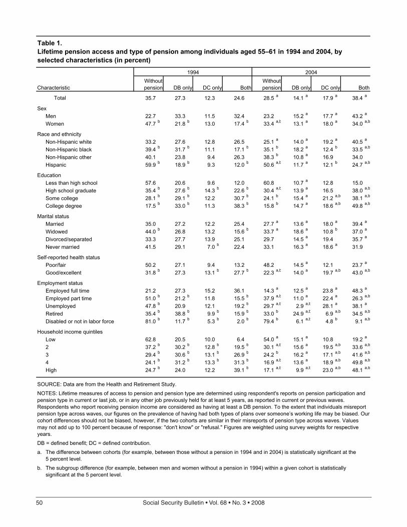
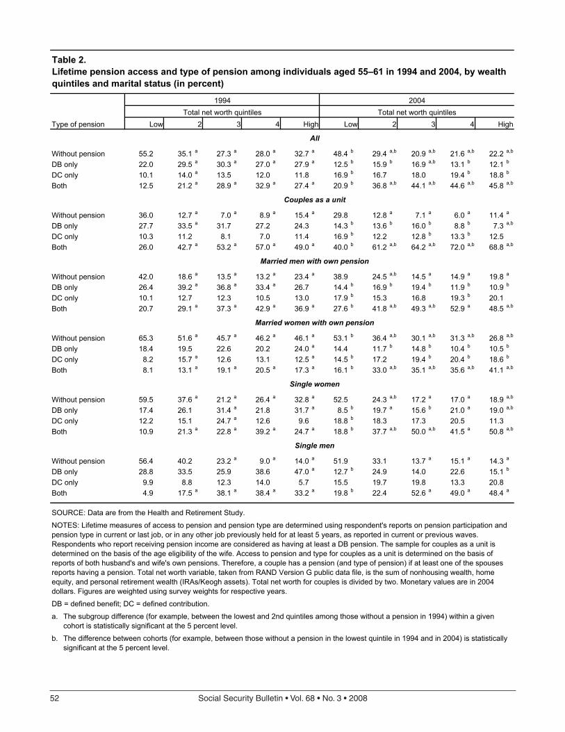
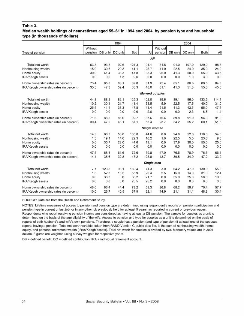
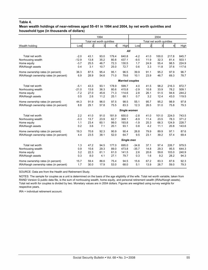
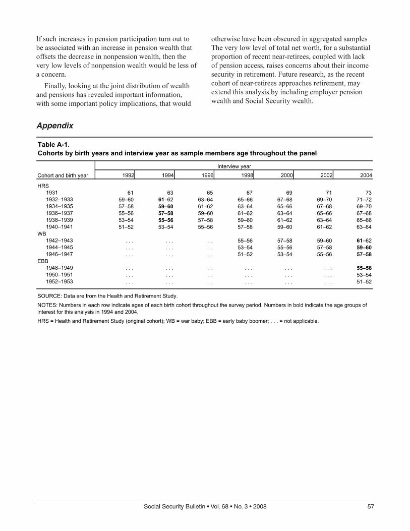
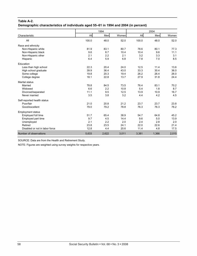
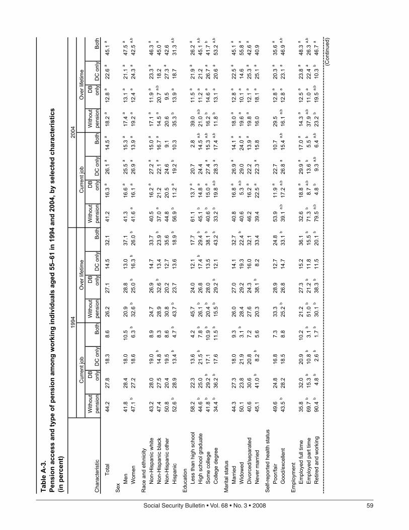
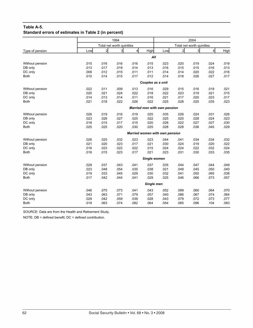
This article examines pension participation and nonpension net worth of two cohorts of near retirees. Particularly, the authors look at people born in 1933 through 1939 who were ages 55–61 in 1994, and the more recent cohort consisting of people of the same age in 2004 who were born in 1943 through 1949. Data are from the Health and Retirement Study, a longitudi-nal, nationally representative survey of older Americans.

Tributes

67 Robert M. Ball: A Life Dedicated to Social Securityby Carolyn Puckett

With the death of Robert Myers Ball at age 93 on January 29, 2008, the Social Security pro-gram lost one of its most committed supporters. In 2001, Ball’s biographer, historian Edward D. Berkowitz, described Ball as “the major non-Congressional player in the history of Social Security in the period between 1950 and the present.”

Social Security BulletinVolume 68 ● Number 3 ● 2008

iv SocialSecurityBulletin•Vol.68•No.3•2008

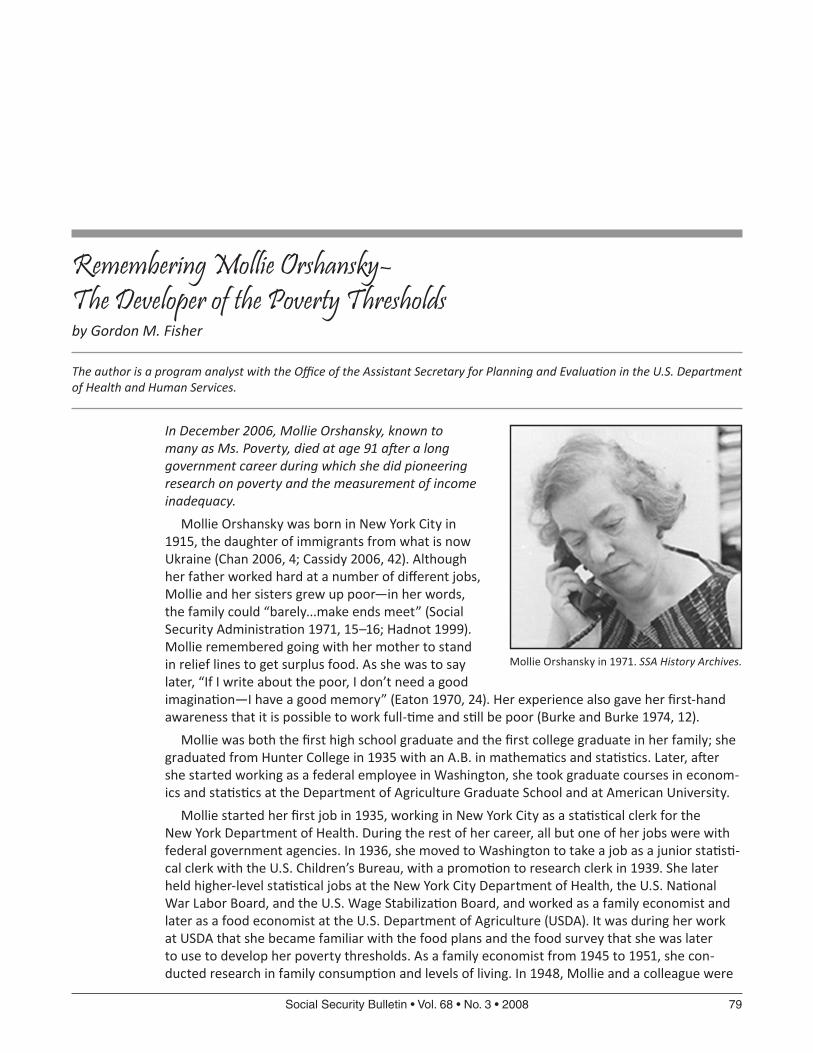
79 Remembering Mollie Orshansky—The Developer of the Poverty Thresholdsby Gordon M. Fisher

In a federal government career that lasted more than four decades, Mollie Orshansky worked for the Children’s Bureau, the Department of Agriculture, the Social Security Administra-tion, and other agencies. While working at the Social Security Administration during the 1960s, she developed the poverty thresholds that became the federal government’s official statistical measure of poverty; her thresholds remain a major feature of the architecture of American social policy and are widely known internationally.

Other

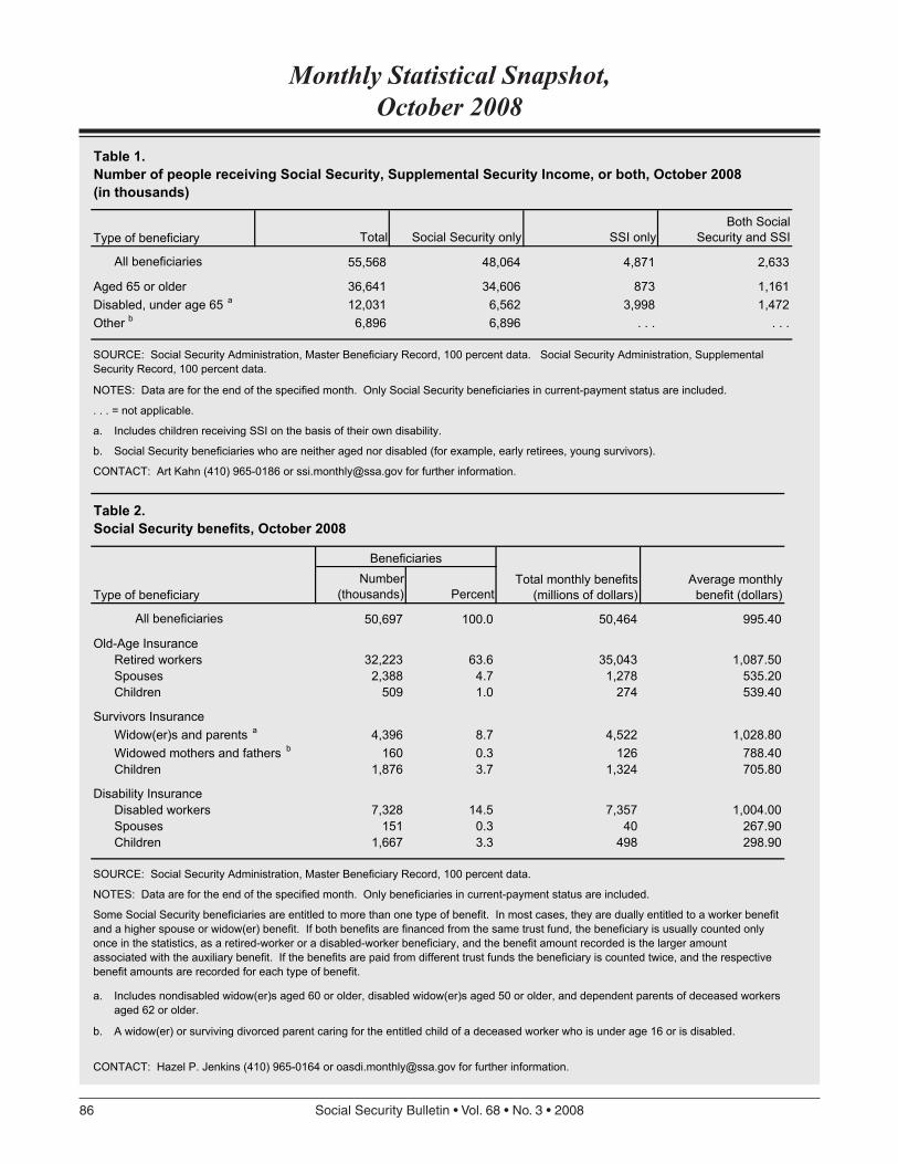
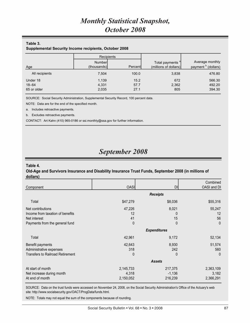
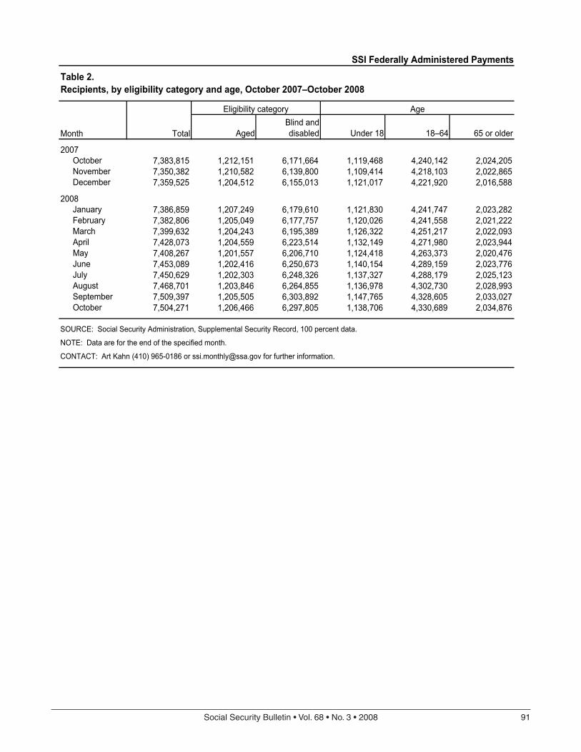
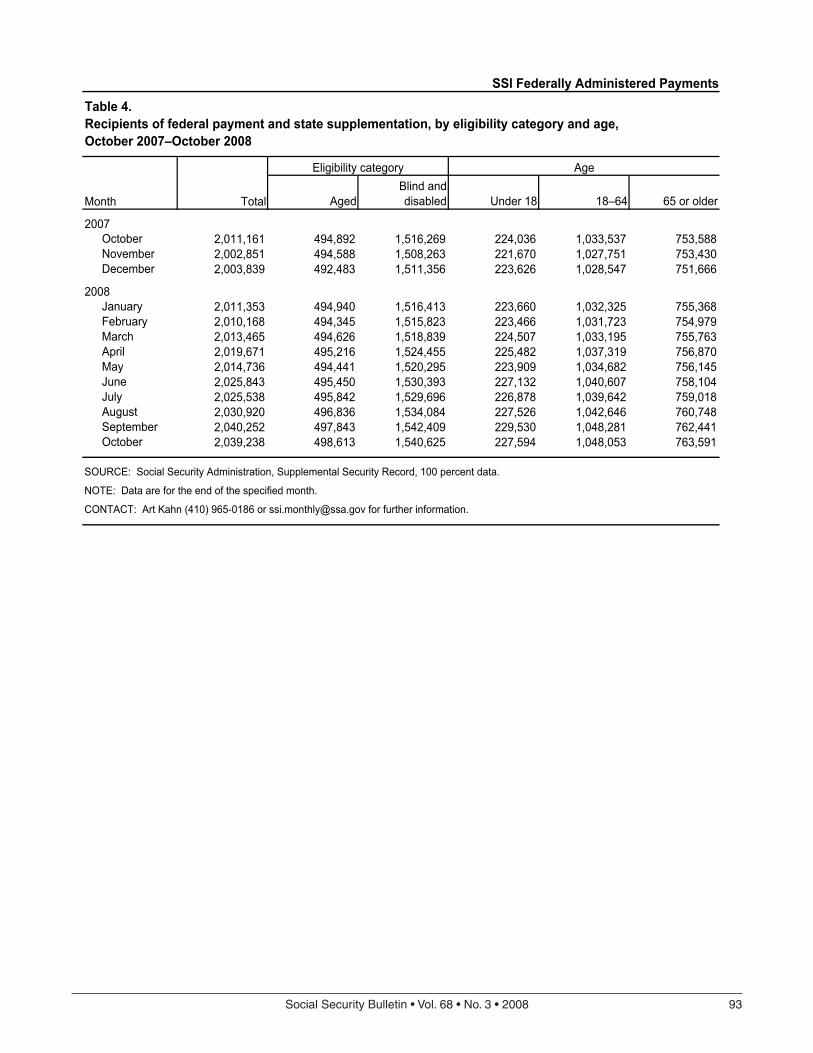
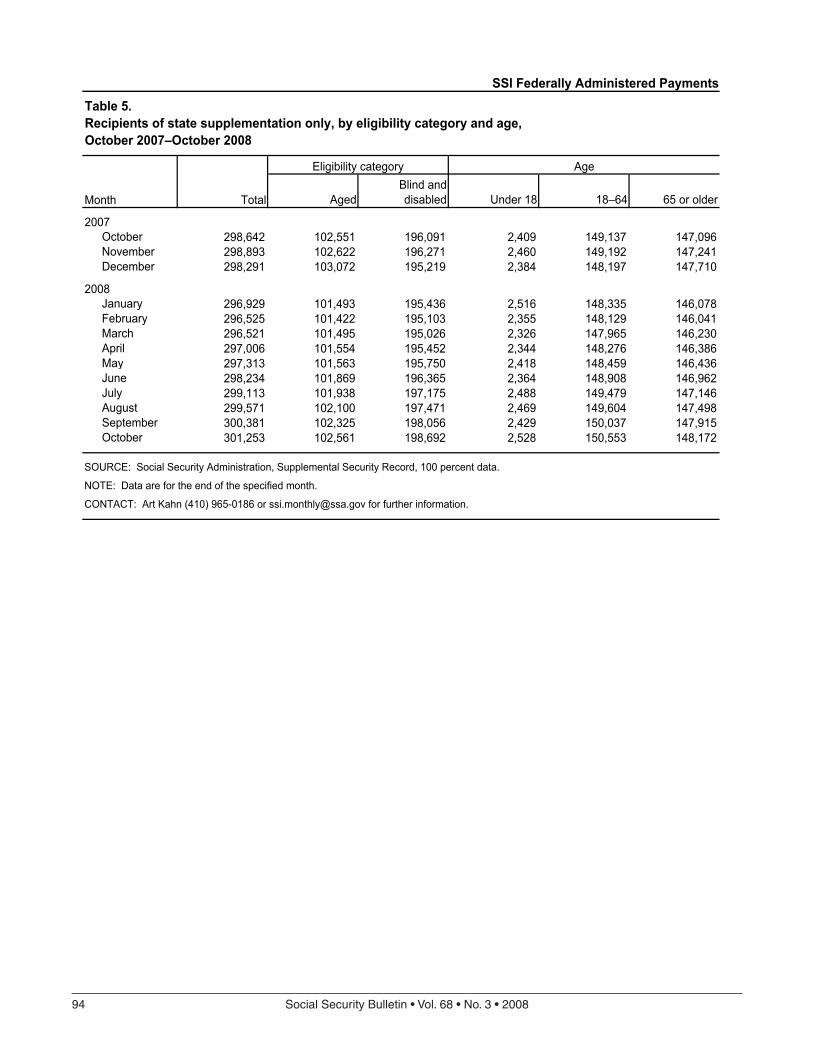
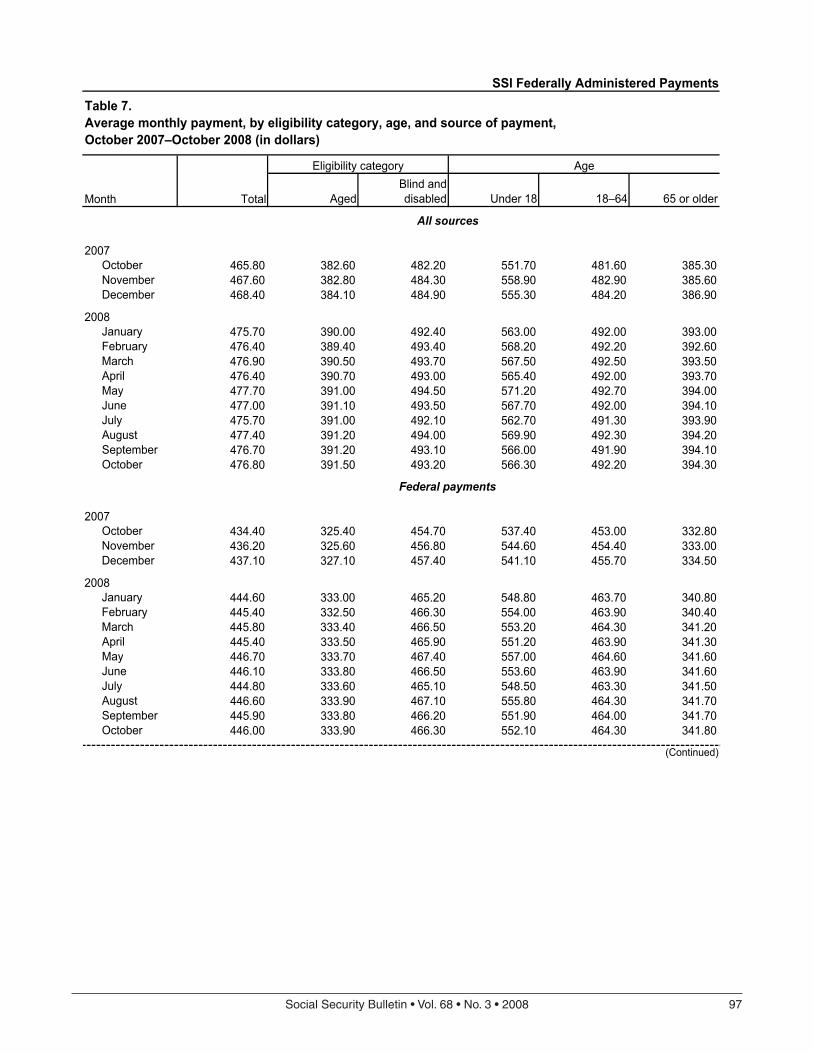
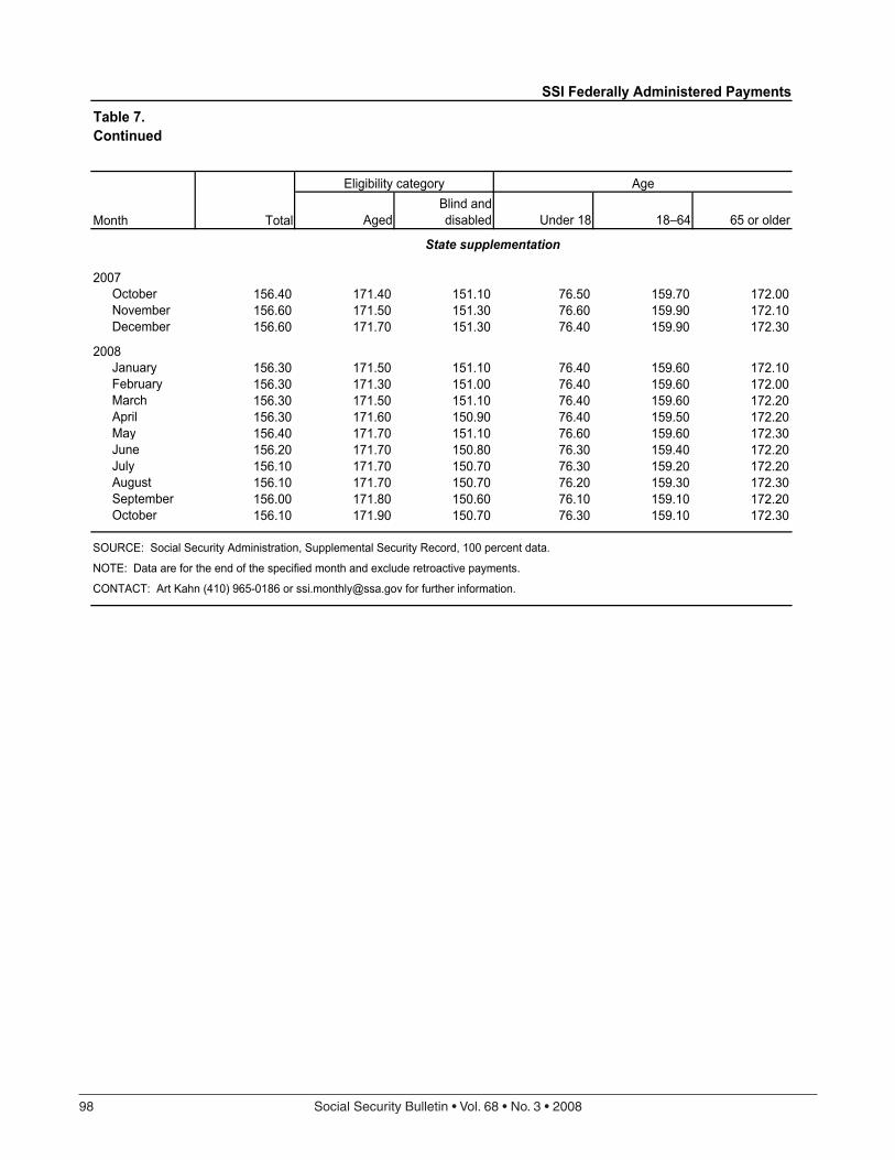
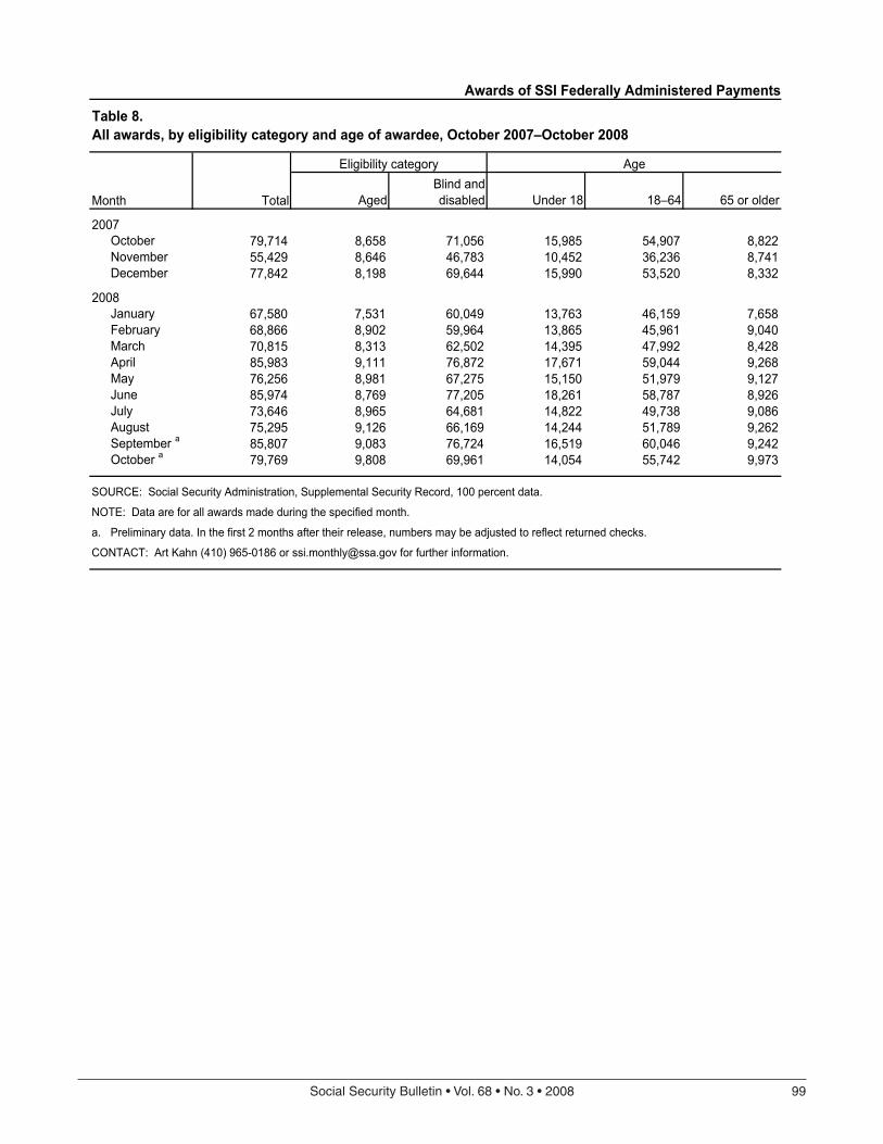
85 OASDI and SSI Snapshot and SSI Monthly Statistics

101 Perspectives–Paper Submission Guidelines

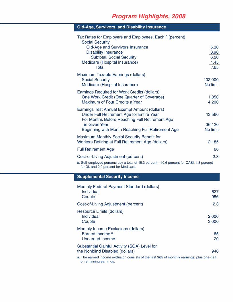
Program Highlights, inside back cover

SocialSecurityBulletin•Vol.68•No.3•2008 1

The Effects of Wage Indexing on Social Security Disability Benefitsby L. Scott Muller

The author is with the Office of Research, Evaluation and Statistics, Office of Retirement and Disability Policy, Social Security Administration.

Summary and IntroductionEconomists David Autor and Mark Duggan have hypothesized that the Social Security Administration’s (SSA’s) use of the average wage index (AWI) in its benefit formula, cou-pled with a widening distribution of income, have created an implicit rise in replacement rates for low-earner disability beneficiaries. They point out that the actual disability benefit received depends implicitly on the individual’s earnings growth relative to the growth of earn-ings for all workers over the benefit calculation period.

This article examines the effect that index-ing using the AWI has had on Social Security benefits. To the extent possible, the article tests the Autor and Duggan hypothesis and attempts to quantify the earnings history and bracket effects using actual earnings histories of disability-insured workers. Whereas Autor and Duggan used earnings at certain percentiles of the earnings distribution to demonstrate the potential effect, this article uses actual earn-ings histories of disability-insured workers to estimate the benefit and replacement rates that each worker would have received if he or she became disabled over the period 1979 to 2004 and to determine if these are, in fact, rising.

This article demonstrates that the distribu-tion of Social Security–reported annual earn-ings is widening, with the highest earners receiving larger increases. Hence, the AWI

may overstate growth for lower earners. Using the Continuous Work History Sample, the article shows that over time replacement rates for many workers have been increasing rela-tive to recent earnings and, as a result, may be increasing incentives to seek disability benefits.

In an alternate approach, a different, more representative index of earnings growth for the majority of workers is used to create a counterfactual, permitting the decomposition of replacement rate changes into the “earnings history” and “bracket” effects identified by Autor and Duggan. Results suggest that both effects have led to higher replacement rates, but the bracket effect appears to contribute most to the trend. Direct comparisons are made between the results from this article, using actual earnings histories, and those obtained in Autor and Duggan’s 2006 article.

Finally, this article analyzes the potential impact of using alternative methods of index-ing on benefits, replacement rates, and pro-gram solvency. For example, an index based on median earnings growth could help sol-vency not only for the disability program, but for the retirement program as well. The analy-sis suggests that progressive indexing could exacerbate problems with incentives to seek benefits and result in a less efficient solution to long-term solvency issues.

Tables presenting detailed data underlying the charts in this article are available as

2 SocialSecurityBulletin•Vol.68•No.3•2008

Appendices B and C at http://www.socialsecurity.gov/ policy/docs/ssb/v68n3/v68n3p1_app.html. These tables may also be requested in hard copy from the author: [email protected].

BackgroundIn the early years of Social Security, the benefit calcu-lation was static, with Congress legislatively granting ad hoc increases in benefits to account for increases in the cost of living or for other reasons. In 1972, Con-gress passed legislation that provided for automatic annual cost-of-living adjustments (COLAs) to benefits based on the Consumer Price Index (CPI). The first annual COLA for Social Security benefits occurred in June 1975. Adjustments were made to the benefit formula by increasing the percentage of the average monthly wage (AMW) applicable to the primary insur-ance amount (PIA) at each bend point in the formula. As the taxable maximum increased each year, an addi-tional bend point was also added to the formula.

Before long it became apparent that this method of adjustment resulted not only in higher benefits, but also in higher real benefits for successive cohorts. Infla-tion increased not only the cost of living and hence the CPI, but generally resulted in higher earnings as well. Higher AMWs and the CPI-adjusted benefit formula resulted in overcompensation for the effects of inflation, increasing real benefits and program costs. Congress debated solutions to the unintended problem and, with the 1977 Amendments to the Social Security Act (P.L. 95-216), legislated a new benefit formula that “decoupled” the COLA from the increase in the wage base.1 After much debate, Congress decided to adjust the benefit for current beneficiaries using the CPI, but to use an average wage index to adjust the earnings history used in computing the initial benefit (PIA).2 Using the CPI to adjust earnings, it was argued, would lead to declining replacement rates for succes-sive cohorts of beneficiaries.3 Adjusting earnings using a wage index would stabilize replacement rates for successive cohorts. Considered somewhat differently, indexing earnings for price changes would provide benefits based on the worker’s share of prior real production, while indexing earnings for wage changes provides benefits based on the individual’s share of current production. In essence, Congress chose to offer benefits based on the standard of living at the time of entitlement, rather than a weighted average of the stan-dard of living over the worker’s working lifetime. At the time, some argued that using wage-indexing in the calculation of benefits would not be sustainable.4

The Decoupled Benefit CalculationThe 1977 amendments were passed to address, among other things, the inadvertent increase in benefits caused by the automatic indexing method enacted in 1972 and begun in June 1975. The 1977 amendments provided for the indexation of the worker’s earnings history to create an average indexed monthly earnings (AIME) measure to replace the AMW.5 The individual’s earn-ings history is indexed to wage levels in the national economy 2 years prior to the year of benefit eligibil-ity6 using a measure of average wages for all work-ers.7 The 1977 amendments also created a new benefit formula for calculating the PIA that uses fixed replace-ment rates (90 percent, 32 percent, and 15 percent) and variable formula bend points that are annually adjusted using a wage index. The formula for comput-ing the maximum family benefit amount (MFBA) was also changed by the 1977 amendments and uses fixed replacement rates and a variable bend point formula that is wage indexed. The national average wage is used to make the wage-indexed adjustments to the individual’s earnings history, the bend points in the PIA and MFBA formulas, and the taxable maximum of annual earnings. The individual’s benefit is calculated at the time of eligibility,8 and the beneficiary receives a COLA in January of each year of entitlement based on changes in the CPI.

The PIA and MFBA benefit formulas from 1979 and 2007 illustrate how wage indexing changes the for-mula over time:

PIA formula1979: 90 percent of the first $180 of AIME +

32 percent of the next $905 of AIME + 15 percent of AIME over $1,085

2007: 90 percent of the first $680 of AIME + 32 percent of the next $4,100 of AIME + 15 percent of AIME over $4,780

MFBA formula9

1979: 150 percent of the first $230 of PIA + 272 percent of the next $102 of PIA + 134 percent of the next $101 of PIA + 175 percent of PIA over $433

2007: 150 percent of the first $869 of PIA + 272 percent of the next $386 of PIA + 134 percent of the next $381 of PIA + 175 percent of PIA over $1,636

Over the years larger portions of earnings (and ben-efits in the MFBA) are subject to the higher replace-ment rates. However, the indexation of the earnings history, coupled with the changes in the formulas, is intended to result in a constant replacement rate for


successive cohorts of entitlements over time, as mea-sured against near-current wage levels.10 This would be the case if earnings grew at the same rate for all individuals, but, as discussed below, it may not be the case if there are changes in the distribution of earnings.

The Autor/Duggan HypothesisDavid Autor and Mark Duggan (2003, 2006) have hypothesized that the benefit formula using the AWI, coupled with a widening distribution of income, has created an implicit rise in replacement rates for low-earner disability beneficiaries. They point out that the actual disability benefit received depends implicitly on the individual’s earnings growth relative to the growth of earnings for all workers over the benefit calculation period. Autor and Duggan’s work pertains specifically to disabled workers, but any impact of wage indexing on benefits also affects the benefit calculation for other beneficiaries, including retired workers.11 In their 2006 article, Autor and Duggan demonstrate the implicit increase in benefits graphically:

Autor and Duggan (2006, 71–96) explain their graph as follows:

Although DI benefits awarded are nominally only a function of a worker’s prior earnings, award amounts are calculated using a wage index equal to mean wage growth economy-wide. Consequently, an individual’s benefit also depends implicitly upon the individual’s earnings growth relative to the growth of earnings for all workers during that worker’s years of employment.

Figure [1] illustrates how this indexation scheme interacts with earnings inequality to raise the replacement rate of low-earnings workers. Line segment A-B-C depicts the benefits schedule of a worker awarded Dis-ability Insurance benefits in 1980 whose wage growth prior to receiving DI exactly paced mean earnings in the economy. The worker’s calculated average indexed monthly earnings amount (AIME) is identical to her 1980 wage. Because the benefits formula replaces between 15 and 90 percent of the marginal dollar (depending on the claim-ant’s AIME), her monthly payment Primary

Figure 1. Illustration of the impact of earnings inequality and indexation on disability insurance benefits in 1980 and 2000

SOURCE:AutorandDuggan(2006).


Insurance Amount (PIA) falls somewhat below her 1980 wage.

Next, consider a worker, represented by line segment A-B-D-E, who is awarded Disability Insurance benefits in 2000. This worker’s nominal wage history in 2000 is identical to that of the beneficiary in 1980 but, in contrast to the 1980 beneficiary, his wage growth during his career lagged con-temporaneous annual average wage growth economy-wide. This worker will receive a higher real Primary Insurance Amount than the worker entering Disability Insurance in 1980. Why? The indexation of the earnings “brackets”—that is, the ranges over which income is replaced at the 90, 32 or 15 per-cent rates—moves these brackets upward, causing a larger share of the worker’s income to be replaced at the 90 or 32 percent rates than would have been the case in 1980. We label this as the “bracket effect” in Figure [1]. Indexation also raises this worker’s DI benefit through a second channel. Because the more recent worker’s entire earnings history is inflated by historical mean wage growth, his average indexed monthly earn-ings amount will actually exceed current earnings (recall that his wage growth has lagged the economy-wide average). We label this as the “earnings history effect” in Fig-ure [1]. Jointly, these two forces—indexation of the earnings brackets and indexation of past earnings—have substantially raised the income replacement rate of low-earnings DI beneficiaries since 1979, when earnings inequality began growing rapidly.

In essence, Autor and Duggan suggest that, if earn-ings rise more slowly for low earners than high earn-ers, over time the AWI will overstate the actual wage growth of low earners, raising the value of their earn-ings in the calculation (“earnings history effect”) and increasing the amount of predisability earnings (or lifetime earnings in the case of retirees) subject to the high replacement rate of the first bend point (“bracket effect”). The combined effect would, over time, increase implicit replacement rates and provide more incentives for low earners to seek disability benefits.12 If the hypothesized effect is actually occurring, the higher benefits and increased incentives to leave the labor force to receive those benefits combine to raise program costs and contribute to long-term solvency problems.

The impact of wage indexing on implicit replace-ment rates may in fact be more complex than that hypothesized by Autor and Duggan. The AWI measure is based only on the wages of persons who have wages during a given year. As employment and labor force participation patterns change, the AWI will be affected. For example, as economic conditions deteriorate, the number of individuals who are unemployed or leave the labor force for an entire year will increase and, since these individuals are not included in the cal-culation of average wages, that measure will tend to show higher average wages than would be the case if the nonearners were included. Hence, average wage figures based only on those who actually have earned income in a year will influence the AWI, most likely overstating wage growth during times of poor eco-nomic conditions. Similarly, during good economic times when marginal workers tend to enter the labor force, their low wages may offset some of the wage gains of the workers with greater labor force attach-ment, tending to hold down the AWI.13

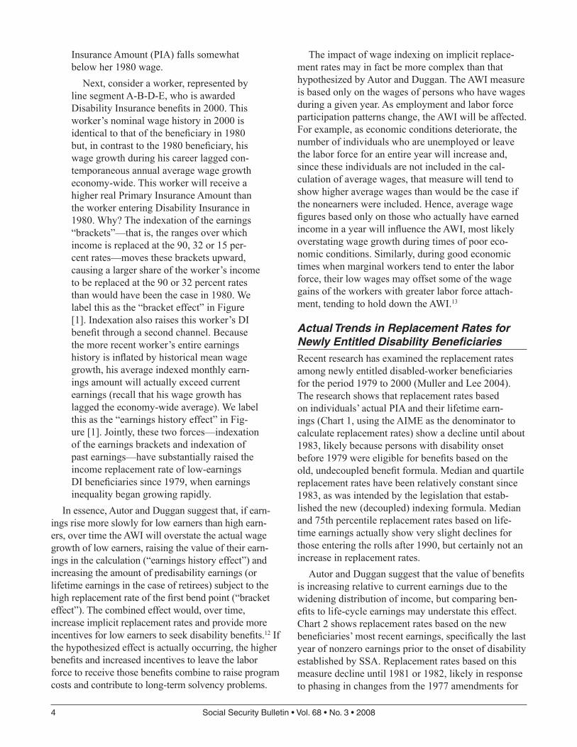
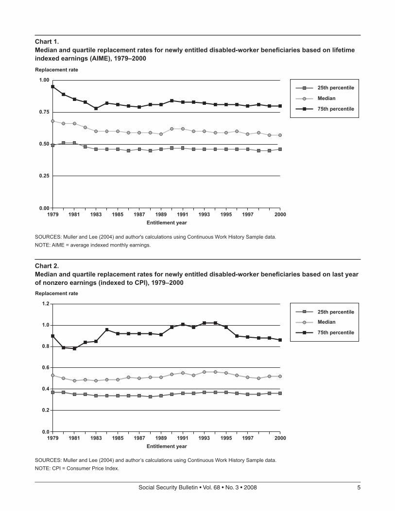
Actual Trends in Replacement Rates for Newly Entitled Disability BeneficiariesRecent research has examined the replacement rates among newly entitled disabled-worker beneficiaries for the period 1979 to 2000 (Muller and Lee 2004). The research shows that replacement rates based on individuals’ actual PIA and their lifetime earn-ings (Chart 1, using the AIME as the denominator to calculate replacement rates) show a decline until about 1983, likely because persons with disability onset before 1979 were eligible for benefits based on the old, undecoupled benefit formula. Median and quartile replacement rates have been relatively constant since 1983, as was intended by the legislation that estab-lished the new (decoupled) indexing formula. Median and 75th percentile replacement rates based on life-time earnings actually show very slight declines for those entering the rolls after 1990, but certainly not an increase in replacement rates.

Autor and Duggan suggest that the value of benefits is increasing relative to current earnings due to the widening distribution of income, but comparing ben-efits to life-cycle earnings may understate this effect. Chart 2 shows replacement rates based on the new beneficiaries’ most recent earnings, specifically the last year of nonzero earnings prior to the onset of disability established by SSA. Replacement rates based on this measure decline until 1981 or 1982, likely in response to phasing in changes from the 1977 amendments for


Entitlement year

Replacement rate

Chart 1.Median and quartile replacement rates for newly entitled disabled-worker beneficiaries based on lifetime indexed earnings (AIME), 1979–2000

SOURCES: Muller and Lee (2004) and author's calculations using Continuous Work History Sample data.NOTE: AIME = average indexed monthly earnings.

25th percentile

Median

75th percentile

200019971995199319911989198719851983198119790.00

0.25

0.50

0.75

1.00

Entitlement year

Replacement rate

Chart 2.Median and quartile replacement rates for newly entitled disabled-worker beneficiaries based on last year of nonzero earnings (indexed to CPI), 1979–2000

SOURCES: Muller and Lee (2004) and author’s calculations using Continuous Work History Sample data.NOTE: CPI = Consumer Price Index.

25th percentile

Median

75th percentile

200019971995199319911989198719851983198119790.0

0.2

0.4

0.6

0.8

1.0

1.2


individuals entitled after 1978, but whose onset of dis-ability occurred prior to 1978. After that, the patterns differ from those observed for the AIME formula-tion. Replacement rates fluctuate after 1985, primarily increasing until 1995 and then generally dropping. There are small increases in the replacement rates for persons entitled to disability in 2000 relative to entitle-ments in the early 1980s. However, the increases only occur for the median and the highest quartile. The rates vary considerably over time and there is no continu-ous increase. This evidence could be consistent with a structural rise in replacement rates, but is clearly not persuasive.

So why do the replacement rates for successive cohorts of disability entitlements not demonstrate the increase in replacement rates hypothesized by Autor and Duggan? Other factors such as economic climate or program could also play a role. There are two com-ponents to the change in actual replacement rates:

Structural change—involving changes in SSA’s • benefit formulation; andBehavioral change—involving changes in the • beneficiary population caused by various factors, including changes in incentives to apply, in demo-graphics, and in the criteria SSA use to determine disability (for example, the change in mental impairments listings implemented in 1986).14

It is difficult to disaggregate the effects of struc-tural and behavioral change in actual experience. For example: as replacement rates rise, those with high replacement rates have more incentive to apply so, all other things being equal, we would expect to see higher rates as the result of both the structural increase and a behavioral response. The behavioral response reflects the possibility that high–replacement rate applicants could seek and receive benefits, thus raising the observed replacement rates. However, after these high–replacement rate individuals are absorbed by the program, we could see replacement rates for new entitlements begin to decline.

Furthermore, the indexing formula itself may mask the true structural change in replacement rates as the numerator (PIA) and denominator (AIME) are both based on wage-indexed values, hence the increases tend to offset one another and the ratio remains stable (that is, using the AWI to index both the numerator and denominator may, in itself, result in the stability of AIME replacement rates over time as both the numera-tor and denominator tend to rise by roughly the same proportion).

Estimating the hypothetical replacement rates of those not actually entering the disability rolls may pro-vide a better idea of what is occurring to replacement rates in the absence of program effects associated with screening and other factors.

MethodologyThis article examines the effect of indexing using the AWI on Social Security benefits. Two distinct meth-ods of assessing the change in replacement rates over time are applied to those who are insured for disability benefits and could apply. Both methods are used to test the Autor and Duggan hypothesis, and one is also used to quantify the earnings history and bracket effects.

Using the Continuous Work History Sample (CWHS), the distribution of annual earnings is assessed to determine whether there is a widening of the income distribution for those insured for disability benefits and whether low earners are receiving smaller wage increases than others. This will confirm whether the effect hypothesized by Autor and Duggan actually exists. The article also assesses the changes in the pro-portion of working-age individuals (aged 18–64) who have positive earnings in a given year, to assess the potential effect that excluding nonearners may have on the AWI.

Two methods are used to assess changes in replace-ment rates over time. Both methods are based on simulations of benefits for disability-insured work-ers using their actual earnings histories and the ben-efit formulas in effect in each year over the period 1979–2004.15 The first method, called “hypothetical replacement rates,” calculates the actual benefit levels and replacement rates that disability-insured workers would receive if they became disabled over the period 1979 to 2004 to see if these are, in fact, rising. Hypo-thetical replacement rates are calculated using three alternative earnings measures: lifetime earnings, most recent year of nonzero earnings, and average earnings over the prior 3 years indexed to the CPI.16 The Autor/Duggan hypothesis suggests that replacement rates are increasing relative to workers’ present or expected earnings, so the recent earnings measures are key to this analysis.

The second method employs an alternate index that is more representative of the earnings growth of nearly all workers. Analysis of CWHS earnings shows that earnings growth is flat for the lowest 80 percent of earners, and that only the top decile or two pro-duce the widening distribution of earnings. Using this


information, a more representative index based on the median earnings growth is used to create a counterfac-tual for each worker, representing what would happen to the individual’s disability benefit if the widening distribution of earnings did not affect the index. This approach also permits one to quantify the “earnings history effect,” the “bracket effect,” and the combined effect on benefits and replacement rates by decom-posing the changes in benefits based on the alternate lifetime earnings calculation and PIA formulation.

Direct comparisons are made between the results from this research using actual earnings histories of disability-insured workers with the hypothetical cases created by Autor and Duggan based on age-specific earnings percentiles generated from historical Current Population Survey data.

The DataThe data employed in this study come from several sources. The indices used in this study come from published sources. The AWI series developed by the Office of the Chief Actuary (OCACT) is used as a measure of mean earnings (SSA 2006a, Table 2.A8). The Consumer Price Index series for Urban Wage Earners and Clerical Workers (CPI-W) is the COLA series used by OCACT to adjust Social Security benefits annually for the change in the cost of living.17 Median earnings data were taken from the histori-cal series of the Annual Statistical Supplement to the Social Security Bulletin (2006a, Table 4.B6). Other series for mean and median earnings were examined and yielded similar results, but limitations on the length of the series led to the above choices for this analysis.

The CWHS is an administrative data file containing a 1 percent sample of all Social Security numbers ever issued. It contains full earnings records enabling the calculation of hypothetical AIMEs and PIAs. It also has information on beneficiary status, allowing the removal of individuals at the time they receive disabil-ity benefits. There are two components to the CWHS: the active file and the inactive file. The active file includes all individuals who have ever had earnings or received a benefit. There is also an inactive file for individuals who have never had any activity with SSA. All data used in this article come from the active file. There are three exclusions from the analysis. Work-ers who actually become disability beneficiaries are dropped from the analysis in the year prior to the year of disability onset. Similarly, workers for whom a date

of death appears on the CWHS are dropped from the analysis in the year prior to the year of death.18 Finally, the analysis of replacement rates includes only work-ers who are insured for disability and are aged 18–61. The age 61 cutoff was used because the majority of workers retire at age 62 and would not have earnings after that age.

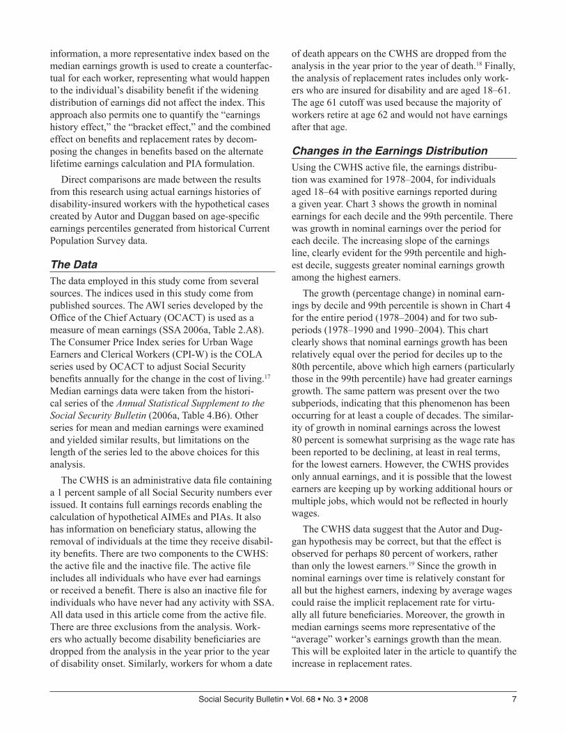
Changes in the Earnings DistributionUsing the CWHS active file, the earnings distribu-tion was examined for 1978–2004, for individuals aged 18–64 with positive earnings reported during a given year. Chart 3 shows the growth in nominal earnings for each decile and the 99th percentile. There was growth in nominal earnings over the period for each decile. The increasing slope of the earnings line, clearly evident for the 99th percentile and high-est decile, suggests greater nominal earnings growth among the highest earners.

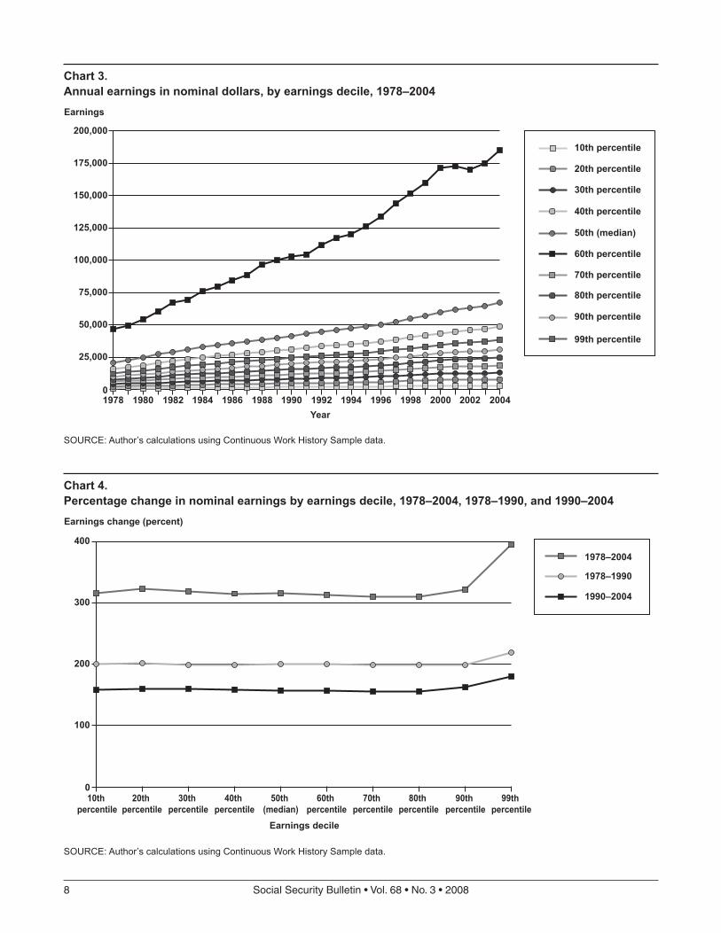
The growth (percentage change) in nominal earn-ings by decile and 99th percentile is shown in Chart 4 for the entire period (1978–2004) and for two sub-periods (1978–1990 and 1990–2004). This chart clearly shows that nominal earnings growth has been relatively equal over the period for deciles up to the 80th percentile, above which high earners (particularly those in the 99th percentile) have had greater earnings growth. The same pattern was present over the two subperiods, indicating that this phenomenon has been occurring for at least a couple of decades. The similar-ity of growth in nominal earnings across the lowest 80 percent is somewhat surprising as the wage rate has been reported to be declining, at least in real terms, for the lowest earners. However, the CWHS provides only annual earnings, and it is possible that the lowest earners are keeping up by working additional hours or multiple jobs, which would not be reflected in hourly wages.

The CWHS data suggest that the Autor and Dug-gan hypothesis may be correct, but that the effect is observed for perhaps 80 percent of workers, rather than only the lowest earners.19 Since the growth in nominal earnings over time is relatively constant for all but the highest earners, indexing by average wages could raise the implicit replacement rate for virtu-ally all future beneficiaries. Moreover, the growth in median earnings seems more representative of the “average” worker’s earnings growth than the mean. This will be exploited later in the article to quantify the increase in replacement rates.


Year

Earnings

Chart 3.Annual earnings in nominal dollars, by earnings decile, 1978–2004

SOURCE: Author’s calculations using Continuous Work History Sample data.

0

25,000

50,000

75,000

100,000

125,000

150,000

175,000

200,000

10th percentile

20th percentile

30th percentile

40th percentile

50th (median)

60th percentile

70th percentile

80th percentile

90th percentile

99th percentile

20042002200019981996199419921990198819861984198219801978

Earnings decile

Earnings change (percent)

Chart 4.Percentage change in nominal earnings by earnings decile, 1978–2004, 1978–1990, and 1990–2004

SOURCE: Author’s calculations using Continuous Work History Sample data.

1978–2004

1978–1990

1990–2004

99th percentile

90th percentile

80th percentile

70th percentile

60th percentile

50th (median)

40th percentile

30th percentile

20th percentile

10th percentile

0

100

200

300

400


Average Wage, Median Earnings, and Price IncreasesThis section makes direct comparisons between the changes over time in measures of average earnings using OCACT’s AWI, median earnings from the Annual Statistical Supplement to the Social Security Bulletin (SSA 2006a), and prices using SSA’s specific calcula-tion of the CPI.20 Chart 5 shows that the pattern of annual percentage changes in mean and median earn-ings and prices is not consistent. In some years, the increase in median earnings exceeds the increase in mean wages, but generally the mean wages show the largest increase, followed by median earnings and then prices. Chart 6 shows the cumulative change in the three measures from 1978 through 2004. Over time, gener-ally larger increases in mean wages have led to widen-ing gaps between the mean and median measures. Both earnings measures have increased substantially more than prices over the period, although not in all years.

The Impact of Nonearners on the Mean and Median Earnings MeasuresAs discussed earlier, the mean and median earnings measures may be biased because nonearners (either

due to unemployment or withdrawal from the labor force for a year or longer, or to trends in labor force participation) are excluded from the calculation. Chart 7 shows the percentage of working-aged per-sons (aged 18–64 in each year) included in the CWHS active file that had positive earnings. The chart shows that the percentage with earnings has been gener-ally trending upward over time. In addition, there are declines in the percentage with positive earnings dur-ing periods of recession (the early 1980s, early 1990s, and after 2000). The decline in the percentage with earnings during recessions varies, from only 1 percent-age point between 1990 and 1992, to nearly 4 percent-age points between 1979 and 1982. The increase in the number of persons without earnings in the year, if included in the calculation, would serve to reduce both the average and the median earnings.21 Thus, excluding individuals who have no earnings in a given year impacts the average wage calculation. Given the upward trend in the proportion of persons with positive earnings over much of the period, it would be difficult to pinpoint the actual number of nonearners to include in the mean and median earnings calculation to estab-lish an alternative population base for calculating the wage index. It also raises questions about how much

Year

Annual change (percent)

Chart 5.Annual percentage change in median earnings, mean earnings (AWI), and in the Consumer Price Index (CPI), 1979–2004

SOURCE: SSA (2006a). NOTE: AWI = average wage index.

0

3

6

9

12

15

Median

Mean (AWI)

CPI

2004200119991997199519931991198919871985198319811979


Year

Workers with earnings (percent)

Chart 7.Percent of workers aged 18–64 with earnings, 1979–2004

SOURCE: Author’s calculations using Continuous Work History Sample active file data.

60

64

68

72

76

80

2004200119991997199519931991198919871985198319811979

Year

Cumulative change (percent)

Chart 6.Cumulative percentage change in median earnings, mean earnings (AWI), and in the Consumer Price Index (CPI), 1978–2004

SOURCE: SSA (2006a). NOTE: AWI = average wage index.

0

50

100

150

200

250

Median

Mean (AWI)

CPI

20042002200019981996199419921990198819861984198219801978


one would want poor (or good) economic conditions to influence benefit calculations.

Hypothetical Replacement Rates for Disability-Insured WorkersIn this section, the CWHS is used to estimate hypo-thetical replacement rates for disability-insured work-ers, that is, the replacement rate that would be obtained if a disability-insured nonbeneficiary were to seek benefits. These replacement rates are not susceptible to some of the problems associated with those for new entitlements, such as the effect of changes in SSA screening criteria on new entrants. The measure is, however, subject to the following limitations:

Absorption onto the disability rolls—if increas-• ing replacement rates induce individuals to leave the labor force for the disability rolls, the replace-ment rates for nonbeneficiary workers will decline over time.Economic cycles—replacement rates based on • recent earnings are influenced by economic cycles, though the overall effect is unknown. Low earnings in economic downturns raise replace-ment rates, and dropping individuals who have

no earnings tends to reduce replacement rates, as higher earners generally have more stable employment.Underlying demographic shifts over time, such as • more women working, women’s earnings rising relative to those for men, an aging workforce, and a shift in the age of peak earnings influence the trends in the distribution of replacement rates for cohorts of insured workers.

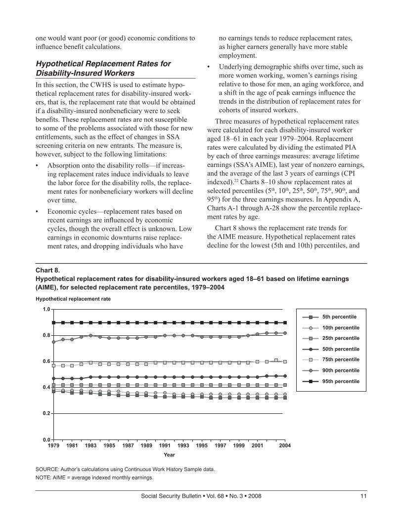
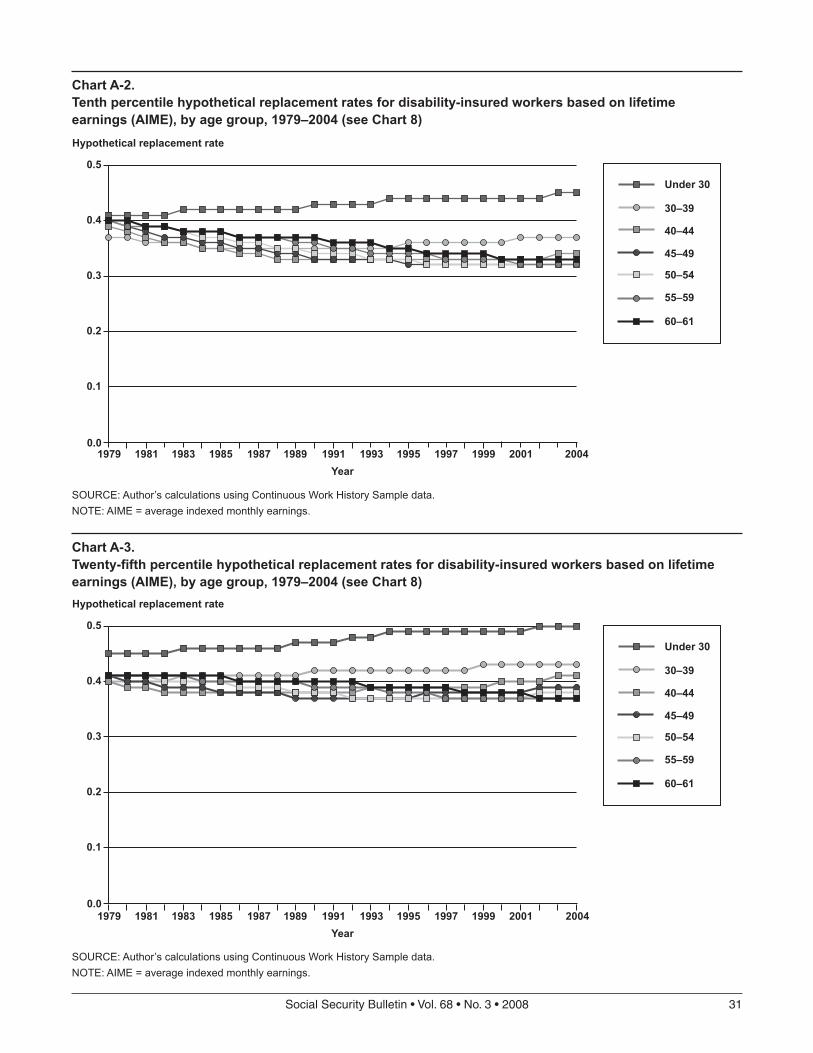
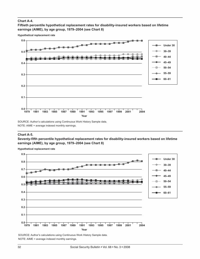
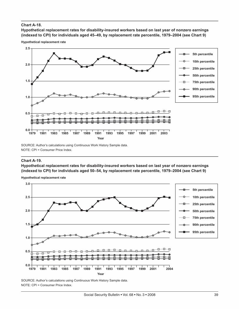
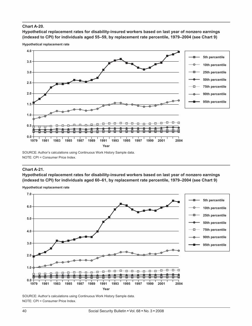
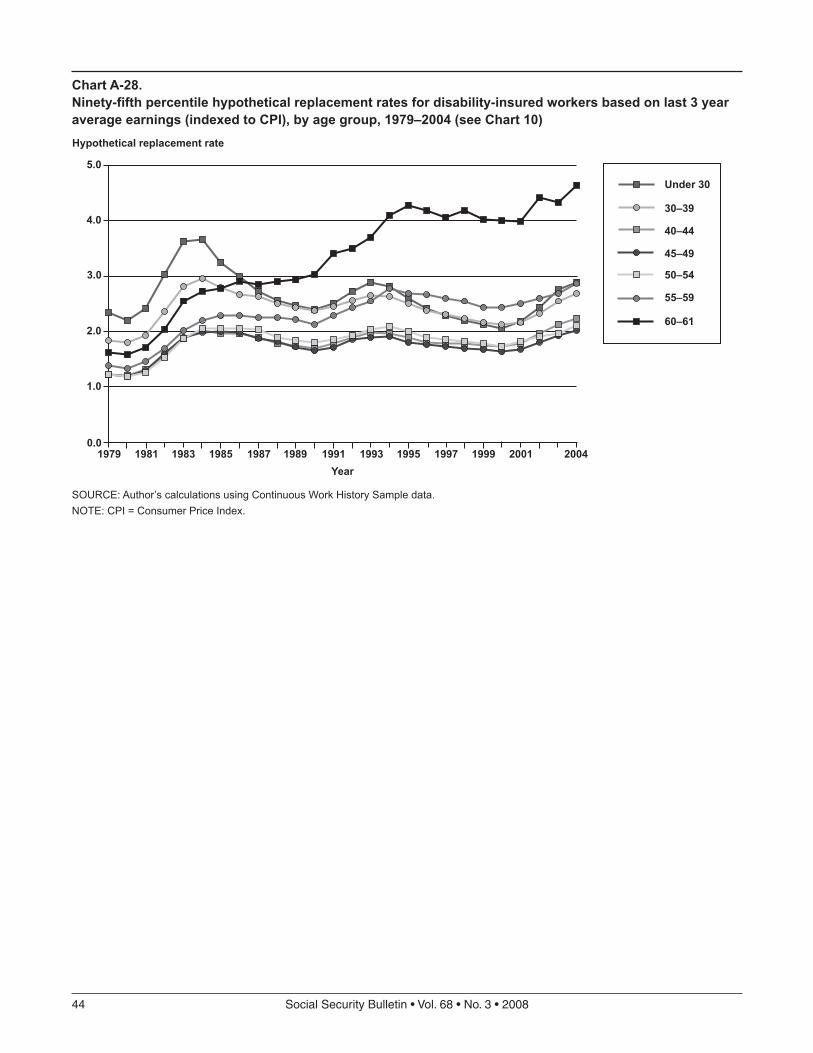
Three measures of hypothetical replacement rates were calculated for each disability-insured worker aged 18–61 in each year 1979–2004. Replacement rates were calculated by dividing the estimated PIA by each of three earnings measures: average lifetime earnings (SSA’s AIME), last year of nonzero earnings, and the average of the last 3 years of earnings (CPI indexed).22 Charts 8–10 show replacement rates at selected percentiles (5th, 10th, 25th, 50th, 75th, 90th, and 95th) for the three earnings measures. In Appendix A, Charts A-1 through A-28 show the percentile replace-ment rates by age.

Chart 8 shows the replacement rate trends for the AIME measure. Hypothetical replacement rates decline for the lowest (5th and 10th) percentiles, and

Year

Hypothetical replacement rate

Chart 8.Hypothetical replacement rates for disability-insured workers aged 18–61 based on lifetime earnings (AIME), for selected replacement rate percentiles, 1979–2004

SOURCE: Author’s calculations using Continuous Work History Sample data.NOTE: AIME = average indexed monthly earnings.

5th percentile

10th percentile

25th percentile

50th percentile

75th percentile

90th percentile

95th percentile

20042001199919971995199319911989198719851983198119790.0

0.2

0.4

0.6

0.8

1.0


increase for those from the median to the 90th percen-tile. Appendix Charts A-1 through A-7, which show replacement rates by age, show that AIME replace-ment rates are dropping for the lowest percentiles, except for those in the youngest age categories. For much of the mid percentiles, replacement rates are fairly stable, as intended by the 1977 legislation, although the younger age groups again show rising replacement rates. In the highest percentiles (90th and 95th), the replacement rates rise for the younger age groups, but tend to decline for the older age groups. The reduction in replacement rates for all but the youngest age group in the 5th and 10th percentiles might be expected because earnings for this high-earning group have been increasing faster than for other groups. Replacement rates for those under age 30 show substantial increases over time at nearly every percentile.23 There is also a slight increase in replace-ment rates for those aged 30–39. This suggests that either entry-level earnings are declining (because earnings generally are inversely related to replacement rates), individuals are entering the labor force at older ages (after age 22, resulting in additional years with no earnings in the AIME calculation), or individuals are working less.

The relatively small increases in replacement rates for some, and the modest increase for many, suggest that the AIME formulation of replacement rates may support the existence of the Autor/Duggan effect, at least for those with lower lifetime earnings and for some age groups. However, as Autor and Duggan contend that benefits represent a larger portion of cur-rent earnings of workers and thus provide incentives to seek disability benefits, formulations of replacement rates based on recent earnings may provide a more accurate picture.

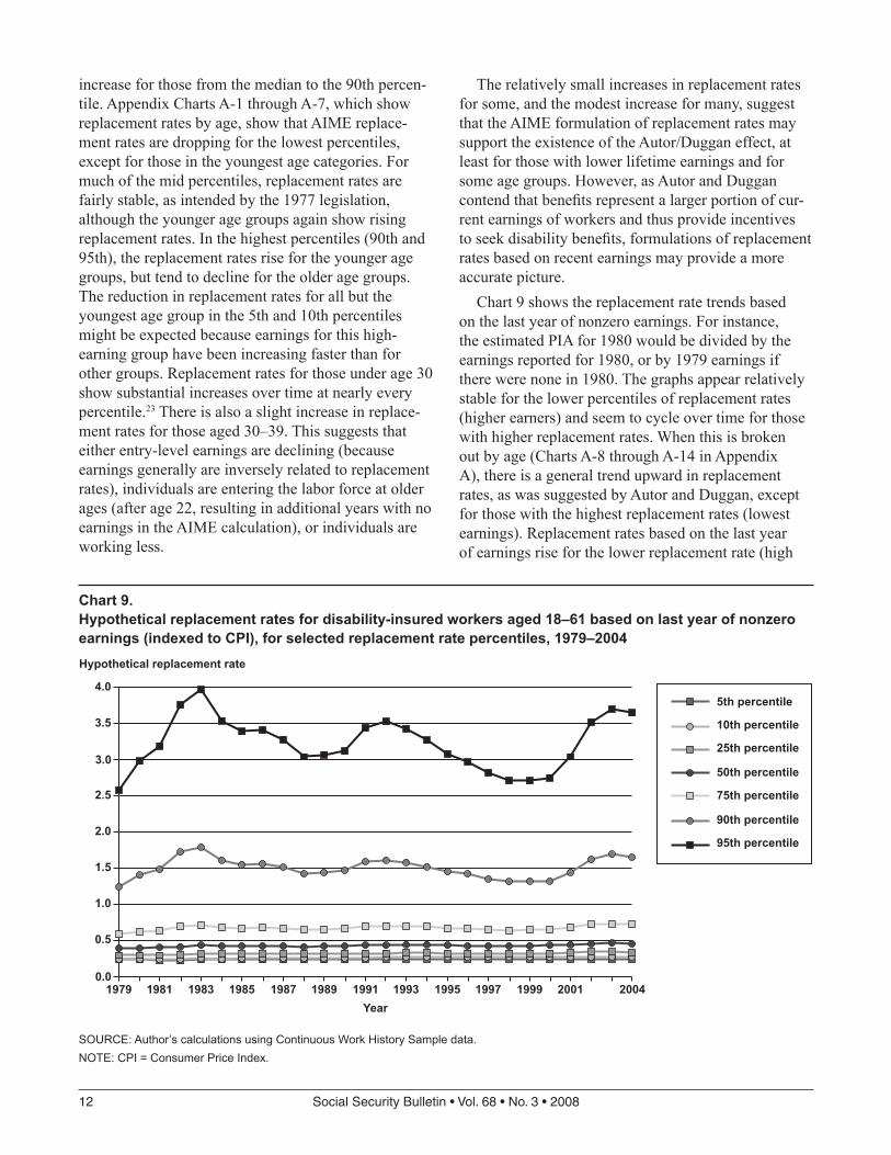
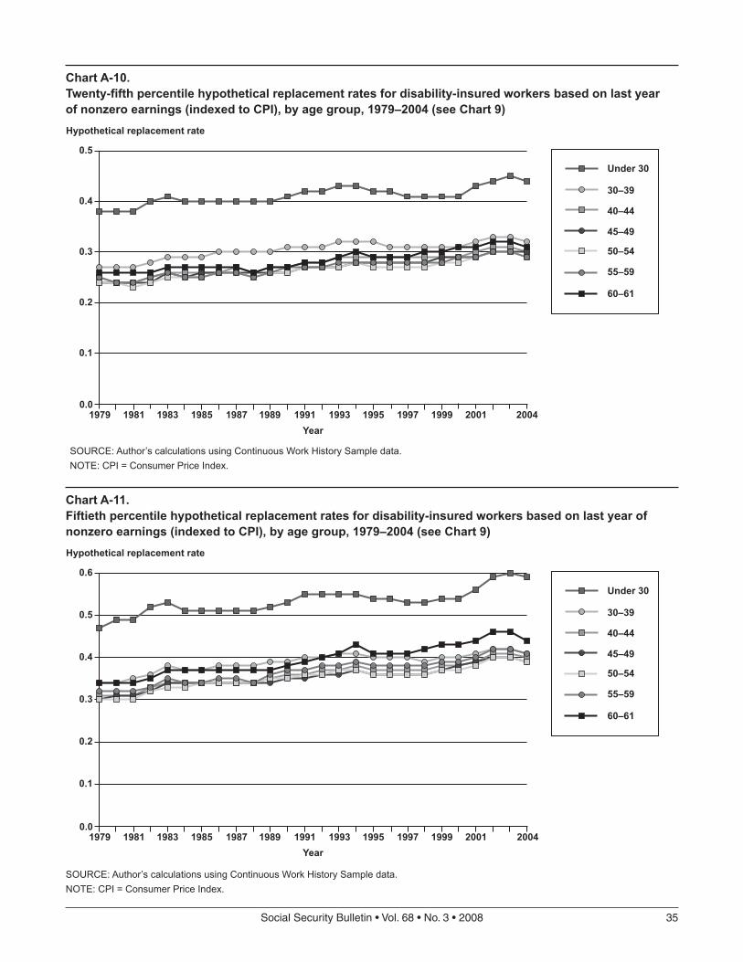
Chart 9 shows the replacement rate trends based on the last year of nonzero earnings. For instance, the estimated PIA for 1980 would be divided by the earnings reported for 1980, or by 1979 earnings if there were none in 1980. The graphs appear relatively stable for the lower percentiles of replacement rates (higher earners) and seem to cycle over time for those with higher replacement rates. When this is broken out by age (Charts A-8 through A-14 in Appendix A), there is a general trend upward in replacement rates, as was suggested by Autor and Duggan, except for those with the highest replacement rates (lowest earnings). Replacement rates based on the last year of earnings rise for the lower replacement rate (high

Year


Chart 9.Hypothetical replacement rates for disability-insured workers aged 18–61 based on last year of nonzero earnings (indexed to CPI), for selected replacement rate percentiles, 1979–2004

SOURCE: Author’s calculations using Continuous Work History Sample data.NOTE: CPI = Consumer Price Index.

0.0

0.5

1.0

1.5

2.0

2.5

3.0

3.5

4.05th percentile

10th percentile

25th percentile

50th percentile

75th percentile

90th percentile

95th percentile

2004200119991997199519931991198919871985198319811979


earner) individuals (5th through 75th percentiles). For the lowest earners with high (90th and 95th percentile) replacement rates, it seems that for most age groups the replacement rates seem to rise and fall over time, with a pattern of high replacement rates in periods of poor economic performance (for example, during the recessions of the early 1980s, early 1990s, and after 2000). The one major exception within the 90th and 95th percentiles is the 60–61 age group, which has a definite upward trend in replacement rates. It is inter-esting that replacement rates for the oldest workers (aged 55–59 and 60–61) increase over the period for most levels, including the highest percentiles. Appen-dix Charts A-15 through A-21 show the trend graphs for each age group, rather than for percentiles, and more clearly show the increase in replacement rates among the older groups.

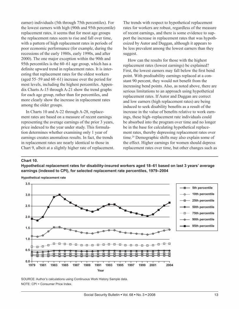
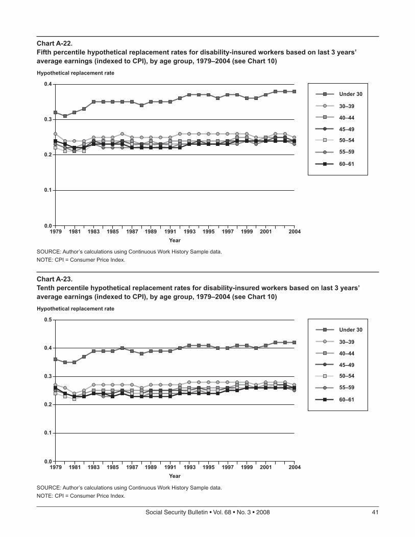
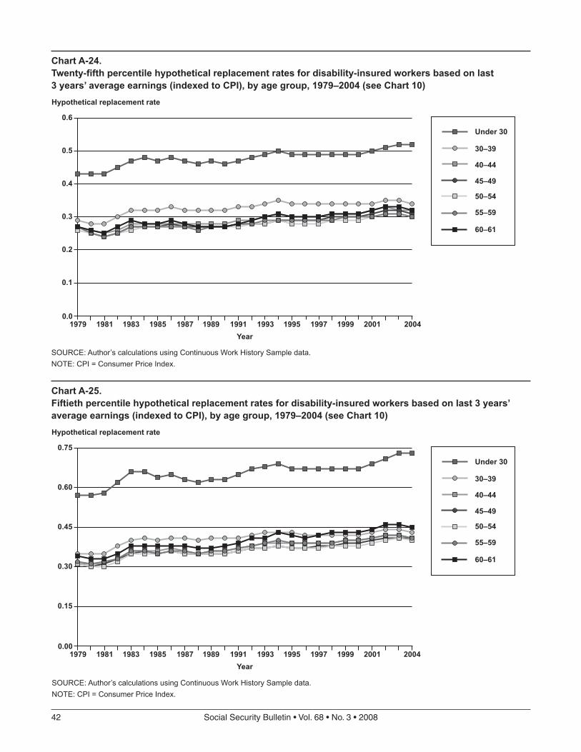
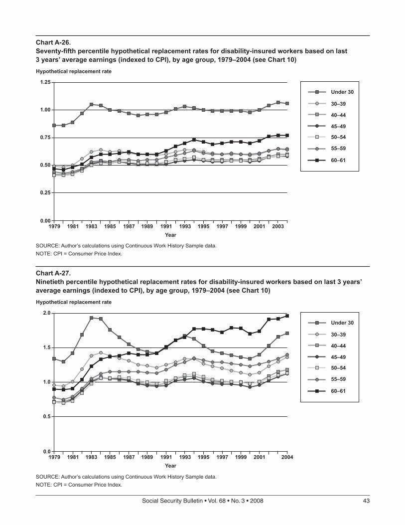
In Charts 10 and A-22 through A-28, replace-ment rates are based on a measure of recent earnings representing the average earnings of the prior 3 years, price indexed to the year under study. This formula-tion determines whether examining only 1 year of earnings creates anomalous results. In fact, the trends in replacement rates are nearly identical to those in Chart 9, albeit at a slightly higher rate of replacement.

The trends with respect to hypothetical replacement rates for workers are robust, regardless of the measure of recent earnings, and there is some evidence to sup-port the increase in replacement rates that was hypoth-esized by Autor and Duggan, although it appears to be less prevalent among the lowest earners than they suggest.

How can the results for those with the highest replacement rates (lowest earnings) be explained? First, the lowest earners may fall below the first bend point. With predisability earnings replaced at a con-stant 90 percent, they would not benefit from the increasing bend points. Also, as noted above, there are serious limitations to an approach using hypothetical replacement rates. If Autor and Duggan are correct and low earners (high replacement rates) are being induced to seek disability benefits as a result of the increase in the value of benefits relative to work earn-ings, these high–replacement rate individuals could be absorbed into the program over time and no longer be in the base for calculating hypothetical replace-ment rates, thereby depressing replacement rates over time.24 Demographic shifts may also explain some of the effect. Higher earnings for women should depress replacement rates over time, but other changes such as

Year


Chart 10.Hypothetical replacement rates for disability-insured workers aged 18–61 based on last 3 years’ average earnings (indexed to CPI), for selected replacement rate percentiles, 1979–2004


0.0

0.5

1.0

1.5

2.0

2.5

3.0

3.55th percentile

10th percentile

25th percentile

50th percentile

75th percentile

90th percentile

95th percentile

2004200119991997199519931991198919871985198319811979


entering the workforce entry at older ages (Compson 2008) and reaching peak earnings at younger ages could result in higher replacement rates.

Assessing the Autor and Duggan Effect by Exploiting the Stability of Median EarningsAs shown earlier in Chart 4, nominal earnings growth from 1978 to 2004 was constant across at least the lowest 80 percent of earners. This suggests that if the wage index reflected this level of earnings growth, the replacement rate increases associated with the widening earnings distribution would be minimized, although those with earnings in the top 20 percent would suffer replacement rate cuts. In this section, the consistency in earnings growth for the lower 80 per-cent of workers is exploited in order to quantify the increase in replacement rates and to decompose the increase into the “earnings history” and “bracket” effects identified by Autor and Duggan.

This is accomplished by constructing a median earnings index (MEI),25 which is arguably more rep-resentative of the earnings growth for the population as it represents the average earnings growth for over 80 percent of earners and tends to eliminate the effect of the widening distribution of earnings. While there are still individual differences in earnings or wage growth from any index, the median earnings index eliminates the “average” effect of the earnings growth differential from the widening distribution of earnings for the population as a whole. Using each individual as his or her own control, or counterfactual, the worker’s replacement rate is calculated using the current AWI formula and a revised formula using the MEI to calcu-late the AIME and PIA.

The decomposition into changes in replacement rates works as follows:

Total effect = (PIAmei (AIMEmei) – PIAawi (AIMEawi)) / AIMEawi

Bracket effect = (PIAmei (AIMEawi) – PIAawi (AIMEawi)) / AIMEawi

Earnings history effect = (PIAawi (AIMEmei) – PIAawi (AIMEawi)) / AIMEawi

Where:PIAawi (AIMEawi) is the current law PIA calcu-

lated from current-law AIME;PIAmei (AIMEmei) is the alternate index PIA cal-

culated from the alternate-index AIME;PIAmei (AIMEawi) is the alternate index PIA cal-

culated from the current-law AIME;

PIAawi (AIMEmei) is the current law PIA calcu-lated from the alternate-index AIME; and

AIMEawi is the current-law AIME and the replace-ment rate denominator.

The difference in the two formulations is the “total effect” on replacement rates associated with the wid-ening of the distribution of earnings. By using the AWI in the calculation of the AIME, and using the AWI and MEI to calculate the bend points for the PIA, the difference between current-law replacement rates and this formulation is a measure of the “bracket” effect identified by Autor and Duggan. Finally, by using the MEI and AWI to compute the AIME and the AWI in the calculation of the PIA, one obtains an estimate of the “earnings history” effect on replacement rates. It is interesting to note that in nearly all cases (97 percent), the total effect as measured by the difference in the AWI and MEI calculations is equal to the earnings his-tory effect plus the bracket effect. There are very few cases in which the changes interact and there is a dis-crepancy between the sum of the bracket and earnings history effects and the total effect, and these “errors” are very small.

This approach is not without its weaknesses. As in the hypothetical replacement rate calculation, there is an absorption effect as the high–replacement rate indi-viduals are induced onto the disability rolls and leave the pool of workers in the analysis. However, this approach minimizes demographic shifts in that each case acts as its own control, or counterfactual. Because the measurements are based on lifetime earnings, the impact of economic cycles is also minimized as the replacement rate denominator is less volatile for all but the youngest workers.

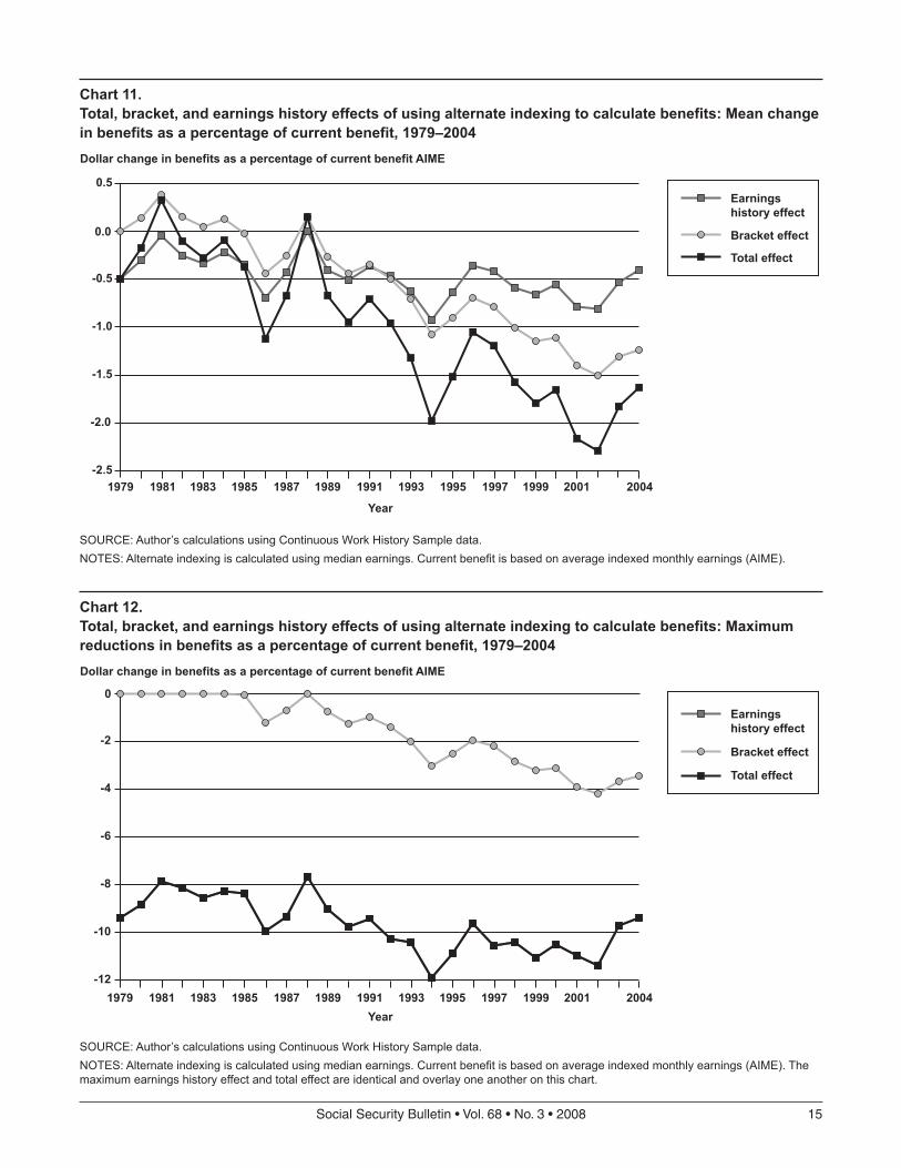
The average effects of the indexing change on replacement rates for the total population are shown in Chart 11. The chart shows a general trend toward greater reductions in replacement rates when using the MEI as a more representative index. The average change is rather small, reaching a maximum reduction in replacement rates of about 2.25 percent of AIME in 2002. The chart also shows that the bracket effect has been the larger contributor to the reduction since the early 1990s, although before then the earnings history effect was larger (and in many years the bracket effect actually resulted in benefit increases).

Chart 12 shows the maximum percentage-point reductions in replacement rates resulting from using MEI over the period. These reductions varied from a low of about 8 percent in 1981 and 1988 to a high of


Year

Dollar change in benefits as a percentage of current benefit AIME

Chart 11.Total, bracket, and earnings history effects of using alternate indexing to calculate benefits: Mean change in benefits as a percentage of current benefit, 1979–2004

SOURCE: Author’s calculations using Continuous Work History Sample data.NOTES: Alternate indexing is calculated using median earnings. Current benefit is based on average indexed monthly earnings (AIME).

-2.5

-2.0

-1.5

-1.0

-0.5

0.0

0.5Earnings history effect

Bracket effect

Total effect

2004200119991997199519931991198919871985198319811979

Year


Chart 12.Total, bracket, and earnings history effects of using alternate indexing to calculate benefits: Maximum reductions in benefits as a percentage of current benefit, 1979–2004

SOURCE: Author’s calculations using Continuous Work History Sample data.NOTES: Alternate indexing is calculated using median earnings. Current benefit is based on average indexed monthly earnings (AIME). Themaximum earnings history effect and total effect are identical and overlay one another on this chart.

-12

-10

-8

-6

-4

-2

0

Earnings history effect

Bracket effect

Total effect

2004200119991997199519931991198919871985198319811979


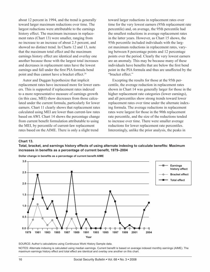
about 12 percent in 1994, and the trend is generally toward larger maximum reductions over time. The largest reductions were attributable to the earnings history effect. The maximum increases in replace-ment rates (Chart 13) were smaller, ranging from no increase to an increase of about 2.5 percent, and showed no distinct trend. In Charts 12 and 13, note that the maximum total effect and the maximum earnings history effect are identical and overlay one another because those with the largest total increases and decreases in replacement rates have the lowest earnings and fall under the first PIA formula bend point and thus cannot have a bracket effect.26

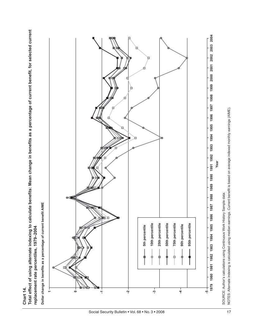
Autor and Duggan hypothesize that implicit replacement rates have increased more for lower earn-ers. This is supported if replacement rates indexed to a more representative measure of earnings growth (in this case, MEI) show decreases from those calcu-lated under the current formula, particularly for lower earners. Chart 11 clearly shows that replacement rates calculated using MEI are lower than current-law rates based on AWI. Chart 14 shows the percentage change from current benefit formulation attributable to using the MEI, by percentile of current-law replacement rates based on the AIME. There is only a slight trend

toward larger reductions in replacement rates over time for the very lowest earners (95th replacement rate percentile) and, on average, the 95th percentile had the smallest reductions in average replacement rates in the latter years. However, as Chart 15 shows, the 95th percentile included individuals with the larg-est maximum reductions in replacement rates, vary-ing between 8 percentage points and 12 percentage points over the period. Clearly the very lowest earners are an anomaly. This may be because many of these individuals have benefits that are below the first bend point in the PIA formula and thus are unaffected by the “bracket effect.”

Excepting the results for those at the 95th per-centile, the average reduction in replacement rates shown in Chart 14 was generally larger for those in the higher replacement rate categories (lower earnings), and all percentiles show strong trends toward lower replacement rates over time under the alternate index-ing formula. The average reductions in replacement rates were largest for those in the 90th replacement rate percentile, and the size of the reductions tended to increase over time. There were smaller average reductions for lower replacement rate percentiles. Interestingly, unlike the prior analysis, the peaks in

Year


Chart 13.Total, bracket, and earnings history effects of using alternate indexing to calculate benefits: Maximum increases in benefits as a percentage of current benefit, 1979–2004

SOURCE: Author’s calculations using Continuous Work History Sample data.NOTES: Alternate indexing is calculated using median earnings. Current benefit is based on average indexed monthly earnings (AIME). Themaximum earnings history effect and total effect are identical and overlay one another on this chart.

0.0

0.5

1.0

1.5

2.0

2.5

3.0Earnings history effect

Bracket effect

Total effect

2004200119991997199519931991198919871985198319811979


-5-4-3-2-101

5th

perc

entil

e

10th

per

cent

ile

25th

per

cent

ile

50th

per

cent

ile

75th

per

cent

ile

90h

perc

entil

e

95th

per

cent

ile

2004

2003

2002

2001

2000

1999

1998

1997

1996

1995

1994

1993

1992

1991

1990

1989

1988

1987

1986

1985

1984

1983

1982

1981

1980

1979

Year

Cha

rt 1

4.To

tal e

ffect

of u

sing

alte

rnat

e in

dexi

ng to

cal

cula

te b

enef

its: M

ean

chan

ge in

ben

efits

as

a pe

rcen

tage

of c

urre

nt b

enef

it, fo

r sel

ecte

d cu

rren

t re

plac

emen

t rat

e pe

rcen

tiles

, 197

9–20

04D

olla

r cha

nge

in b

enef

its a

s a

perc

enta

ge o

f cur

rent

ben

efit

AIM

E

SO

UR

CE

: Aut

hor’s

cal

cula

tions

usi

ng C

ontin

uous

Wor

k H

isto

ry S

ampl

e da

ta.

NO

TES

: Alte

rnat

e in

dexi

ng is

cal

cula

ted

usin

g m

edia

n ea

rnin

gs. C

urre

nt b

enef

it is

bas

ed o

n av

erag

e in

dexe

d m

onth

ly e

arni

ngs

(AIM

E).


-12

-10-8-6-4-20

5th

perc

entil

e

10th

per

cent

ile

25th

per

cent

ile

50th

per

cent

ile

75th

per

cent

ile

90h

perc

entil

e

95th

per

cent

ile

2004

2003

2002

2001

2000

1999

1998

1997

1996

1995

1994

1993

1992

1991

1990

1989

1988

1987

1986

1985

1984

1983

1982

1981

1980

1979

Year

Cha

rt 1

5.To

tal e

ffect

of u

sing

alte

rnat

e in

dexi

ng to

cal

cula

te b

enef

its: M

axim

um re

duct

ion

in b

enef

its a

s a

perc

enta

ge o

f cur

rent

ben

efit,

for s

elec

ted

cu

rren

t rep

lace

men

t rat

e pe

rcen

tiles

, 197

9–20

04D

olla

r cha

nge

in b

enef

its a

s a

perc

enta

ge o

f cur

rent

ben

efit

AIM

E

SO

UR

CE

: Aut

hor’s

cal

cula

tions

usi

ng C

ontin

uous

Wor

k H

isto

ry S

ampl

e da

ta.

NO

TES

: Alte

rnat

e in

dexi

ng is

cal

cula

ted

usin

g m

edia

n ea

rnin

gs. C

urre

nt b

enef

it is

bas

ed o

n av

erag

e in

dexe

d m

onth

ly e

arni

ngs

(AIM

E).


replacement rates do not coincide with economic recessions.27

This analysis of alternative replacement rate for-mulations does not seem to provide strong support for Autor and Duggan’s hypothesis that wage index-ing has a greater effect on the lowest earners. The earlier approach, analyzing hypothetical replacement rates based on recent earnings, led to a similar find-ing. However, examining the maximum reduction in replacement rates by percentile (Chart 15) reveals that the largest reductions for individuals occur in the highest replacement rate category—that is, for the low-est earners. This indicates that the incentives created by increased replacement rates may be greatest for some of the lowest earners. Moreover, the maximum reductions in replacement rates decline as the level of replacement rates falls (that is, they are smaller for those with higher earnings).

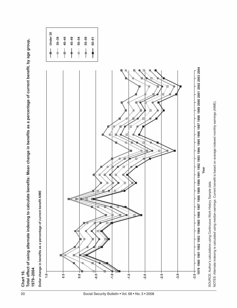
The alternate replacement rate formulation was also examined to assess differences by age. The first approach, hypothetical replacement rates, showed increased replacement rates for all age groups, with a particularly large increase for lower earners aged 60–61. This is confirmed by the alternate index-ing approach (Chart 16). Recall that a decline in MEI replacement rates relative to AWI indicates an implicit rise in current-law rates. Those aged 60–61 had the largest reduction in replacement rates under the alter-nate formulation, but the difference between this and the other age groups was considerably smaller than that found when using the hypothetical replacement rate approach. The latter result may be due to changes over time in the age of peak earnings for succes-sive cohorts, which the alternate indexing approach minimizes.

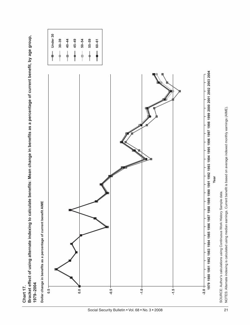
In decomposing the total effect into the bracket and earnings history effects, the analysis shows that the trend toward higher replacement rates is produced by the bracket effect (Chart 17), while the larger reduc-tions for older workers (larger increase in replacement rates under current law) is attributable to the earnings history effect (Chart 18). Moreover, there is very little trend to the earnings history effect; it seems to cycle, but not synchronously with economic cycles.

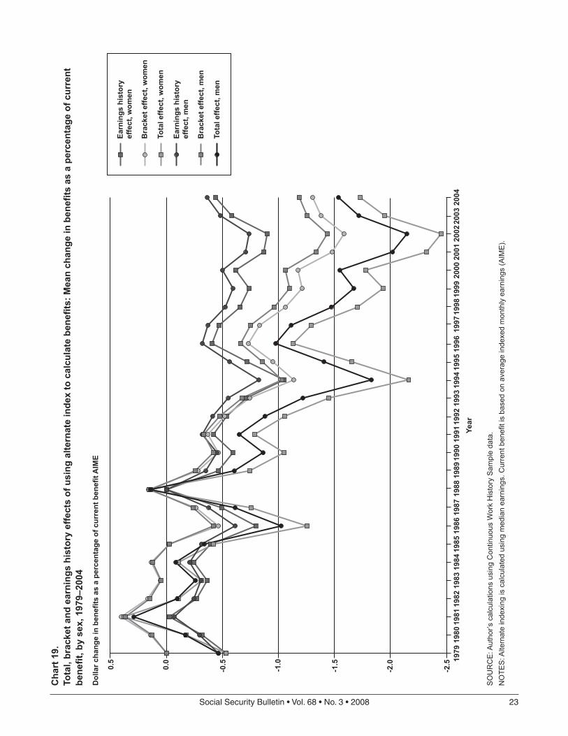
The changes in replacement rates for men and women are shown in Chart 19. Women have larger reductions in replacement rates under the alternate MEI formula, and hence have been benefiting more from the implicit increase in replacement rates. This is likely because women tend to have lower earn-ings and thus higher replacement rates than men, and

those with higher replacement rates tend to have larger reductions.

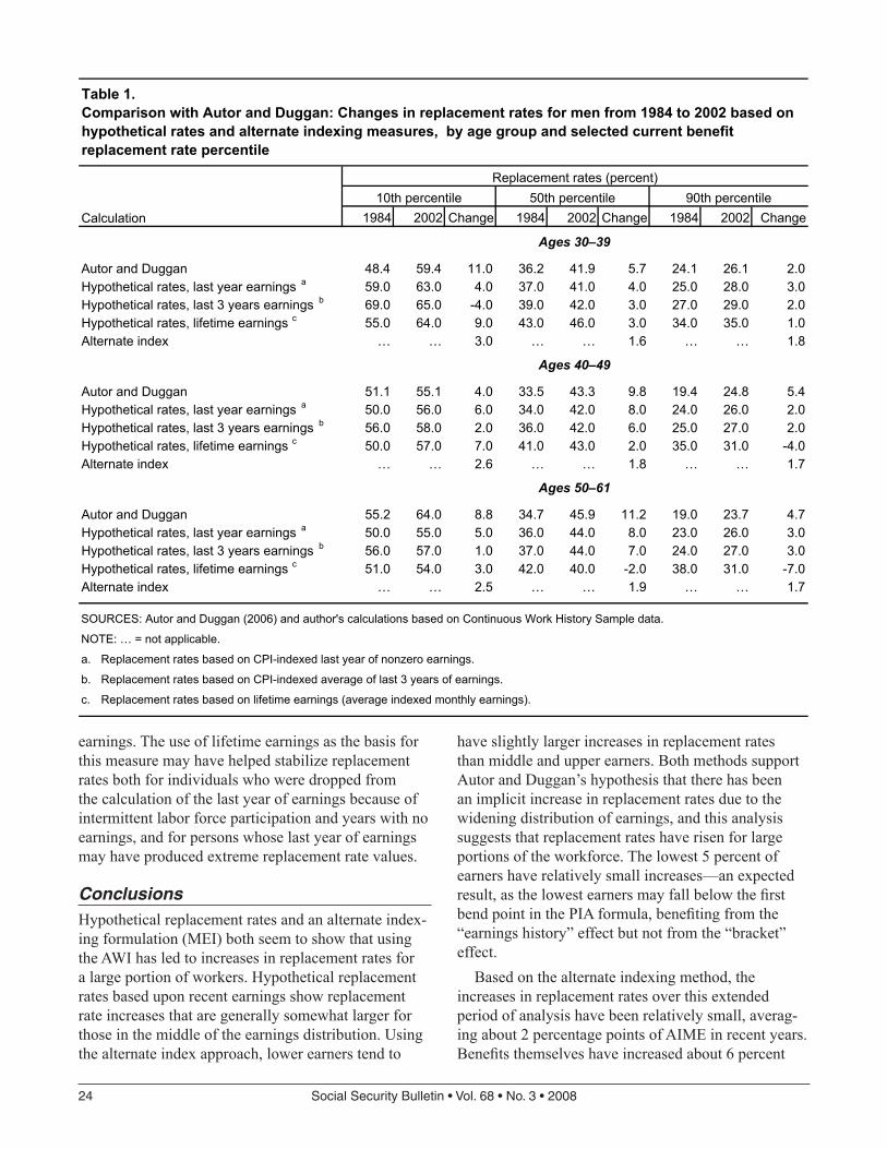
Comparisons to Autor and Duggan ResultsIn Table 2 of their “Crisis” article, Autor and Duggan (2006) provide estimates of replacement rate changes for men between 1984 and 2002 based on the overall distribution of earnings. Table 1 below provides simi-lar estimates based on the calculations in this article. As with Autor and Duggan (2006), which bases its estimates on age-specific percentiles of earnings, the calculations in Table 1 are based on replacement rates for individuals by age-specific percentiles of lifetime earnings (AIME). Because the replacement rates based on recent earnings are so volatile,28 the median replacement rate for individuals whose AIME is within 5 percent (plus or minus) of the percentile value of AIME was used (see the data table appendix available in the online version of this article for a more detailed data presentation).

This article uses actual earnings histories of disability-insured workers to compute replacement rates based on recent earnings. Table 1 shows that the results of this approach are generally consistent with Autor and Duggan’s use of historical percentiles of earnings, although the effects estimated here are gener-ally somewhat smaller than those estimated by Autor and Duggan, at least in the two older age groups.29 Replacement rates based on lifetime earnings (AIME) are also shown and, despite the congressional intent to stabilize replacement rates, the youngest group (aged 30–39) and lowest earners (10th percentile of age-specific AIME) see replacement rates increase over time. The result for men aged 30–39 is consistent with earlier analysis; however, the AIME replace-ment rates for the 10th percentile of AIME (the high replacement rate percentiles) seem to be fairly stable overall in the earlier analysis (Chart 8), perhaps indi-cating a difference between men and women.

The alternate index does not produce directly analo-gous results to those generated by Autor and Dug-gan, but change over time can be estimated using a difference-in-differences approach using the estimates of the “total effect” on replacement rates for 1984 and 2004. This measure also shows replacement rates rising over time, although with very small differences by age. Interestingly, using this approach, the lowest earners (10th percentile) receive greater increases than those in the 50th and 90th percentiles, which was not the case with hypothetical replacement rates for recent


-3.5

-3.0

-2.5

-2.0

-1.5

-1.0

-0.50.0

0.5

1.0

Und

er 3

0

30–3

9

40–4

4

45–4

9

50–5

4

55–5

9

60–6

1

2004

2003

2002

2001

2000

1999

1998

1997

1996

1995

1994

1993

1992

1991

1990

1989

1988

1987

1986

1985

1984

1983

1982

1981

1980

1979

Year

Cha

rt 1

6.To

tal e

ffect

of u

sing

alte

rnat

e in

dexi

ng to

cal

cula

te b

enef

its: M

ean

chan

ge in

ben

efits

as

a pe

rcen

tage

of c

urre

nt b

enef

it, b

y ag

e gr

oup,

19

79–2

004

Dol

lar c

hang

e in

ben

efits

as

a pe

rcen

tage

of c

urre

nt b

enef

it A

IME

SO

UR

CE

: Aut

hor’s

cal

cula

tions

usi

ng C

ontin

uous

Wor

k H

isto

ry S

ampl

e da

ta.

NO

TES

: Alte

rnat

e in

dexi

ng is

cal

cula

ted

usin

g m

edia

n ea

rnin

gs. C

urre

nt b

enef

it is

bas

ed o

n av

erag

e in

dexe

d m

onth

ly e

arni

ngs

(AIM

E).


-2.0

-1.5

-1.0

-0.50.0

0.5

Und

er 3

0

30–3

9

40–4

4

45–4

9

50–5

4

55–5

9

60–6

1

2004

2003

2002

2001

2000

1999

1998

1997

1996

1995

1994

1993

1992

1991

1990

1989

1988

1987

1986

1985

1984

1983

1982

1981

1980

1979

Year

Dol

lar c

hang

e in

ben

efits

as

a pe

rcen

tage

of c

urre

nt b

enef

it A

IME

Cha

rt 1

7.B

rack

et e

ffect

of u

sing

alte

rnat

e in

dexi

ng to

cal

cula

te b

enef

its: M

ean

chan

ge in

ben

efits

as

a pe

rcen

tage

of c

urre

nt b

enef

it, b

y ag

e gr

oup,

19

79–2

004

SO

UR

CE

: Aut

hor’s

cal

cula

tions

usi

ng C

ontin

uous

Wor

k H

isto

ry S

ampl

e da

ta.

NO

TES

: Alte

rnat

e in

dexi

ng is

cal

cula

ted

usin

g m

edia

n ea

rnin

gs. C

urre

nt b

enef

it is

bas

ed o

n av

erag

e in

dexe

d m

onth

ly e

arni

ngs

(AIM

E).


-2.0

-1.5

-1.0

-0.50.0

0.5

Und

er 3

0

30–3

9

40–4

4

45–4

9

50–5

4

55–5

9

60–6

1

2004

2003

2002

2001

2000

1999

1998

1997

1996

1995

1994

1993

1992

1991

1990

1989

1988

1987

1986

1985

1984

1983

1982

1981

1980

1979

Year

Dol

lar c

hang

e in

ben

efits

as

a pe

rcen

tage

of c

urre

nt b

enef

it A

IME

Cha

rt 1

8.Ea

rnin

gs h

isto

ry e

ffect

of u

sing

alte

rnat

e in

dexi

ng to

cal

cula

te b

enef

its: M

ean

chan

ge in

ben

efits

as

a pe

rcen

tage

of c

urre

nt b

enef

it, b

y ag

e gr

oup,

197

9–20

04

SO

UR

CE

: Aut

hor’s

cal

cula

tions

usi

ng C

ontin

uous

Wor

k H

isto

ry S

ampl

e da

ta.

NO

TES

: Alte

rnat

e in

dexi

ng is

cal

cula

ted

usin

g m

edia

n ea

rnin

gs. C

urre

nt b

enef

it is

bas

ed o

n av

erag

e in

dexe

d m

onth

ly e

arni

ngs

(AIM

E).


-2.5

-2.0

-1.5

-1.0

-0.50.0

0.5

Earn

ings

his

tory

ef

fect

, wom

en

Bra

cket

effe

ct, w

omen

Tota

l effe

ct, w

omen

Earn

ings

his

tory

ef

fect

, men

Bra

cket

effe

ct, m

en

Tota

l effe

ct, m

en

2004

2003

2002

2001

2000

1999

1998

1997

1996

1995

1994

1993

1992

1991

1990

1989

1988

1987

1986

1985

1984

1983

1982

1981

1980

1979

Year

Dol

lar c

hang

e in

ben

efits

as

a pe

rcen

tage

of c

urre

nt b

enef

it A

IME

Cha

rt 1

9.To

tal,

brac

ket a

nd e

arni

ngs

hist

ory

effe

cts

of u

sing

alte

rnat

e in

dex

to c

alcu

late

ben

efits

: Mea

n ch

ange

in b

enef

its a

s a

perc

enta

ge o

f cur

rent

be

nefit

, by

sex,

197

9–20

04

SO

UR

CE

: Aut

hor’s

cal

cula

tions

usi

ng C

ontin

uous

Wor

k H

isto

ry S

ampl

e da

ta.

NO

TES

: Alte

rnat

e in

dexi

ng is

cal

cula

ted

usin

g m

edia

n ea

rnin

gs. C

urre

nt b

enef

it is

bas

ed o

n av

erag

e in

dexe

d m

onth

ly e

arni

ngs

(AIM

E).


earnings. The use of lifetime earnings as the basis for this measure may have helped stabilize replacement rates both for individuals who were dropped from the calculation of the last year of earnings because of intermittent labor force participation and years with no earnings, and for persons whose last year of earnings may have produced extreme replacement rate values.

ConclusionsHypothetical replacement rates and an alternate index-ing formulation (MEI) both seem to show that using the AWI has led to increases in replacement rates for a large portion of workers. Hypothetical replacement rates based upon recent earnings show replacement rate increases that are generally somewhat larger for those in the middle of the earnings distribution. Using the alternate index approach, lower earners tend to

have slightly larger increases in replacement rates than middle and upper earners. Both methods support Autor and Duggan’s hypothesis that there has been an implicit increase in replacement rates due to the widening distribution of earnings, and this analysis suggests that replacement rates have risen for large portions of the workforce. The lowest 5 percent of earners have relatively small increases—an expected result, as the lowest earners may fall below the first bend point in the PIA formula, benefiting from the “earnings history” effect but not from the “bracket” effect.

Based on the alternate indexing method, the increases in replacement rates over this extended period of analysis have been relatively small, averag-ing about 2 percentage points of AIME in recent years. Benefits themselves have increased about 6 percent

Table 1.Comparison with Autor and Duggan: Changes in replacement rates for men from 1984 to 2002 based on hypothetical rates and alternate indexing measures, by age group and selected current benefit replacement rate percentile

Calculation

Replacement rates (percent)10th percentile 50th percentile 90th percentile

1984 2002 Change 1984 2002 Change 1984 2002 Change

Ages 30–39

Autor and Duggan 48.4 59.4 11.0 36.2 41.9 5.7 24.1 26.1 2.0Hypothetical rates, last year earnings a 59.0 63.0 4.0 37.0 41.0 4.0 25.0 28.0 3.0Hypothetical rates, last 3 years earnings b 69.0 65.0 -4.0 39.0 42.0 3.0 27.0 29.0 2.0Hypothetical rates, lifetime earnings c 55.0 64.0 9.0 43.0 46.0 3.0 34.0 35.0 1.0Alternate index … … 3.0 … … 1.6 … … 1.8

Ages 40–49

Autor and Duggan 51.1 55.1 4.0 33.5 43.3 9.8 19.4 24.8 5.4Hypothetical rates, last year earnings a 50.0 56.0 6.0 34.0 42.0 8.0 24.0 26.0 2.0Hypothetical rates, last 3 years earnings b 56.0 58.0 2.0 36.0 42.0 6.0 25.0 27.0 2.0Hypothetical rates, lifetime earnings c 50.0 57.0 7.0 41.0 43.0 2.0 35.0 31.0 -4.0Alternate index … … 2.6 … … 1.8 … … 1.7

Ages 50–61

Autor and Duggan 55.2 64.0 8.8 34.7 45.9 11.2 19.0 23.7 4.7Hypothetical rates, last year earnings a 50.0 55.0 5.0 36.0 44.0 8.0 23.0 26.0 3.0Hypothetical rates, last 3 years earnings b 56.0 57.0 1.0 37.0 44.0 7.0 24.0 27.0 3.0Hypothetical rates, lifetime earnings c 51.0 54.0 3.0 42.0 40.0 -2.0 38.0 31.0 -7.0Alternate index … … 2.5 … … 1.9 … … 1.7

SOURCES: Autor and Duggan (2006) and author's calculations based on Continuous Work History Sample data.

NOTE: … = not applicable.

a. Replacement rates based on CPI-indexed last year of nonzero earnings.

b. Replacement rates based on CPI-indexed average of last 3 years of earnings.

c. Replacement rates based on lifetime earnings (average indexed monthly earnings).


over what they would have been had a more represen-tative index, or a more equal distribution of earnings prevailed. Hypothetical replacement rates based on recent earnings suggest larger increases than other measures, especially for moderate earners. The decom-position suggests that the “bracket” effect produces the trend toward lower replacement rates, although the “earnings history” effect reduces replacement rates for all cohorts.

This analysis strongly suggests the effects on replacement rates are smaller than those estimated by Autor and Duggan. In fact, the impact over time on replacement rates for those of advanced age (that is, aged 60–61) seems to be as large, or perhaps larger, than the impact of the change in the earnings distribu-tion. The increase in replacement rates for the lowest earners (highest replacement rate percentiles) seems to be smaller than that observed for some other levels of earnings. Overall, the magnitude of the increases in replacement rates, on average, does not seem to offer large incentives to leave work for disability benefits, although results show there are some individuals for whom the increases are much larger (as measured by the maximum changes to replacement rates). The impact of advanced age, as mentioned above, does suggest the effect identified by Autor and Duggan may induce more individuals to retire early and take reduced retirement benefits.

The extent to which this trend toward higher implicit replacement rates continues depends on a number of factors, including a continued widening of the distribution of earnings. Another potential factor is the amount of income that is considered in the average wage index and median earnings calculations. Recent changes have excluded health insurance premiums and money paid into pretax spending accounts for medi-cal and child care expenditures. These changes could result in a narrowing or a widening of the distribution of earnings, depending on the behavioral response at various levels of earned income.

Implications for PolicyThe foregoing analysis suggests that Autor and Dug-gan are correct in their hypothesis that replacement rates are rising due to the widening distribution of income, although the increase may not be as great as their estimates suggested. This finding is important for a number of reasons, perhaps most importantly because it has implications for solvency and policy proposals that have been made to address Social Secu-rity’s future. It is necessary to consider the impact of

wage indexing both from a program cost perspective and from a behavioral perspective where individual incentives could be further distorted. This section will discuss some of the implications of the current AWI indexing and the increase in replacement rates in the context of solvency and policy proposals.

A number of solvency proposals have focused on altering the indexing of earnings in the benefit for-mula. One proposes replacing the AWI with the CPI to index earnings, which would achieve solvency but would also result in falling replacement rates over time. Progressive indexing has also been proposed, under which earnings below a threshold level are wage indexed, and earnings above that threshold are price indexed. Progressive wage indexing would continue the implicit replacement rate creep identified by Autor and Duggan for those low earners subject to wage indexing. This could continue to increase incentives for these low earners to seek disability benefits (or to retire at earlier ages).

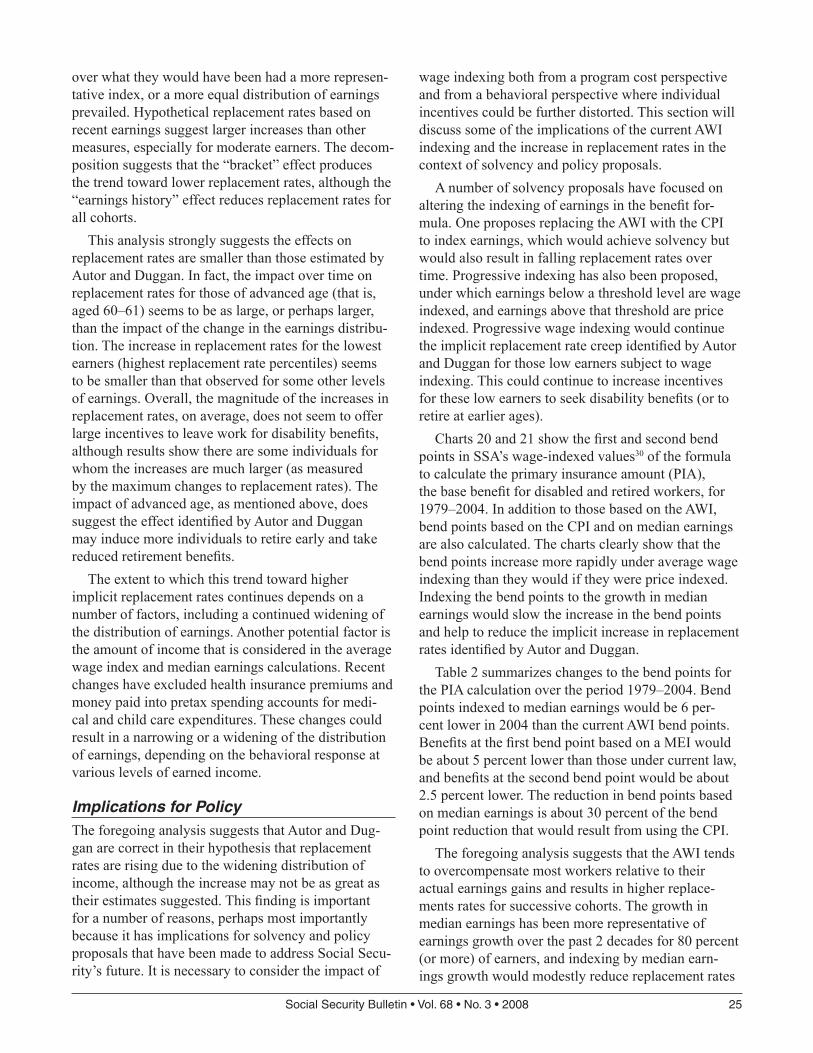
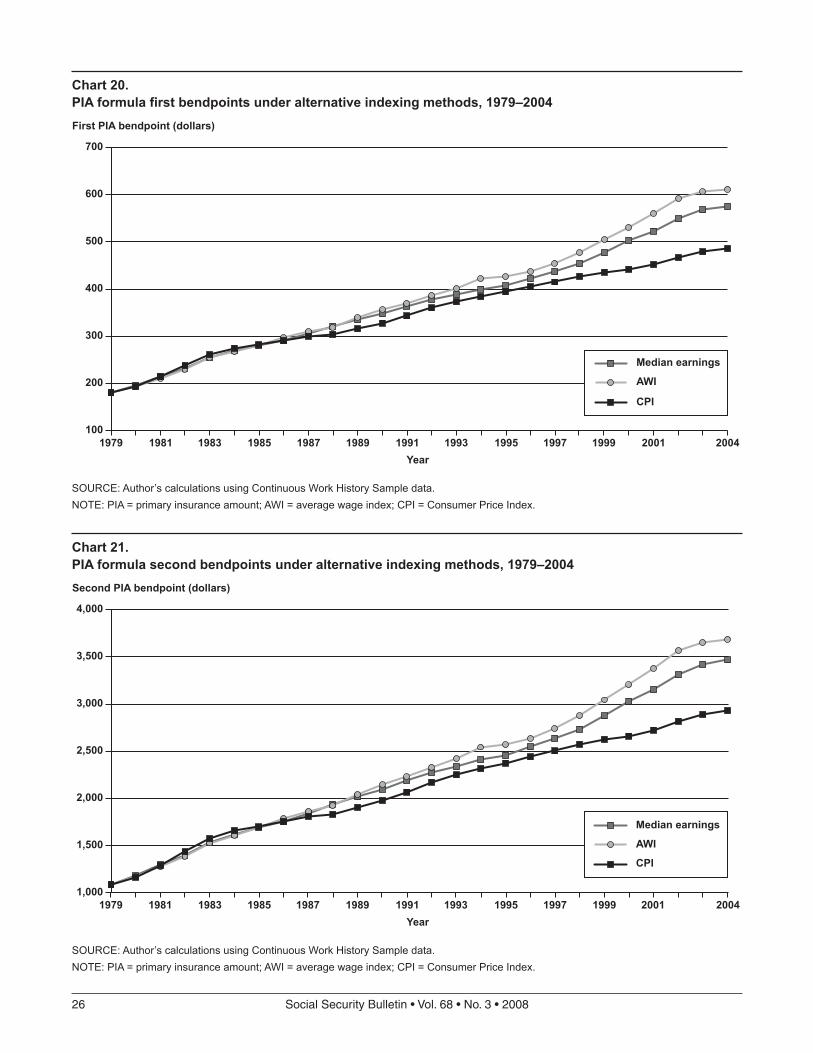
Charts 20 and 21 show the first and second bend points in SSA’s wage-indexed values30 of the formula to calculate the primary insurance amount (PIA), the base benefit for disabled and retired workers, for 1979–2004. In addition to those based on the AWI, bend points based on the CPI and on median earnings are also calculated. The charts clearly show that the bend points increase more rapidly under average wage indexing than they would if they were price indexed. Indexing the bend points to the growth in median earnings would slow the increase in the bend points and help to reduce the implicit increase in replacement rates identified by Autor and Duggan.

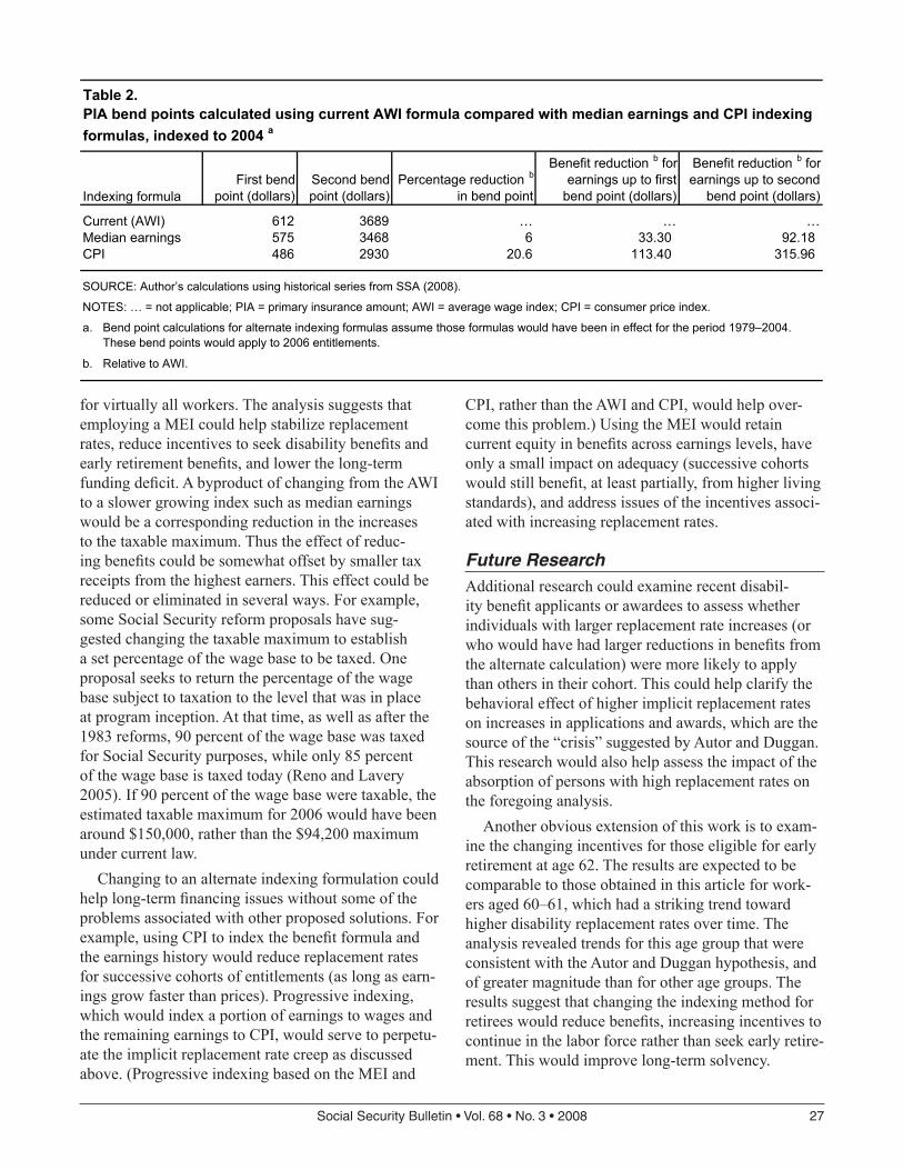
Table 2 summarizes changes to the bend points for the PIA calculation over the period 1979–2004. Bend points indexed to median earnings would be 6 per-cent lower in 2004 than the current AWI bend points. Benefits at the first bend point based on a MEI would be about 5 percent lower than those under current law, and benefits at the second bend point would be about 2.5 percent lower. The reduction in bend points based on median earnings is about 30 percent of the bend point reduction that would result from using the CPI.

The foregoing analysis suggests that the AWI tends to overcompensate most workers relative to their actual earnings gains and results in higher replace-ments rates for successive cohorts. The growth in median earnings has been more representative of earnings growth over the past 2 decades for 80 percent (or more) of earners, and indexing by median earn-ings growth would modestly reduce replacement rates


100

200

300

400

500

600

700

Median earnings

AWI

CPI

2004200119991997199519931991198919871985198319811979Year

First PIA bendpoint (dollars)

Chart 20.PIA formula first bendpoints under alternative indexing methods, 1979–2004

SOURCE: Author’s calculations using Continuous Work History Sample data. NOTE: PIA = primary insurance amount; AWI = average wage index; CPI = Consumer Price Index.

1,000

1,500

2,000

2,500

3,000

3,500

4,000

Median earnings

AWI

CPI

2004200119991997199519931991198919871985198319811979Year

Second PIA bendpoint (dollars)

Chart 21.PIA formula second bendpoints under alternative indexing methods, 1979–2004

SOURCE: Author’s calculations using Continuous Work History Sample data. NOTE: PIA = primary insurance amount; AWI = average wage index; CPI = Consumer Price Index.


for virtually all workers. The analysis suggests that employing a MEI could help stabilize replacement rates, reduce incentives to seek disability benefits and early retirement benefits, and lower the long-term funding deficit. A byproduct of changing from the AWI to a slower growing index such as median earnings would be a corresponding reduction in the increases to the taxable maximum. Thus the effect of reduc-ing benefits could be somewhat offset by smaller tax receipts from the highest earners. This effect could be reduced or eliminated in several ways. For example, some Social Security reform proposals have sug-gested changing the taxable maximum to establish a set percentage of the wage base to be taxed. One proposal seeks to return the percentage of the wage base subject to taxation to the level that was in place at program inception. At that time, as well as after the 1983 reforms, 90 percent of the wage base was taxed for Social Security purposes, while only 85 percent of the wage base is taxed today (Reno and Lavery 2005). If 90 percent of the wage base were taxable, the estimated taxable maximum for 2006 would have been around $150,000, rather than the $94,200 maximum under current law.

Changing to an alternate indexing formulation could help long-term financing issues without some of the problems associated with other proposed solutions. For example, using CPI to index the benefit formula and the earnings history would reduce replacement rates for successive cohorts of entitlements (as long as earn-ings grow faster than prices). Progressive indexing, which would index a portion of earnings to wages and the remaining earnings to CPI, would serve to perpetu-ate the implicit replacement rate creep as discussed above. (Progressive indexing based on the MEI and

CPI, rather than the AWI and CPI, would help over-come this problem.) Using the MEI would retain current equity in benefits across earnings levels, have only a small impact on adequacy (successive cohorts would still benefit, at least partially, from higher living standards), and address issues of the incentives associ-ated with increasing replacement rates.

Future ResearchAdditional research could examine recent disabil-ity benefit applicants or awardees to assess whether individuals with larger replacement rate increases (or who would have had larger reductions in benefits from the alternate calculation) were more likely to apply than others in their cohort. This could help clarify the behavioral effect of higher implicit replacement rates on increases in applications and awards, which are the source of the “crisis” suggested by Autor and Duggan. This research would also help assess the impact of the absorption of persons with high replacement rates on the foregoing analysis.

Another obvious extension of this work is to exam-ine the changing incentives for those eligible for early retirement at age 62. The results are expected to be comparable to those obtained in this article for work-ers aged 60–61, which had a striking trend toward higher disability replacement rates over time. The analysis revealed trends for this age group that were consistent with the Autor and Duggan hypothesis, and of greater magnitude than for other age groups. The results suggest that changing the indexing method for retirees would reduce benefits, increasing incentives to continue in the labor force rather than seek early retire-ment. This would improve long-term solvency.

Table 2.PIA bend points calculated using current AWI formula compared with median earnings and CPI indexing formulas, indexed to 2004 a

Indexing formulaFirst bend

point (dollars)Second bend point (dollars)

Percentage reduction b

in bend point

Benefit reduction b forearnings up to first

bend point (dollars)

Benefit reduction b for earnings up to second

bend point (dollars)

Current (AWI) 612 3689 … … …Median earnings 575 3468 6 33.30 92.18CPI 486 2930 20.6 113.40 315.96

SOURCE: Author’s calculations using historical series from SSA (2008).

NOTES: … = not applicable; PIA = primary insurance amount; AWI = average wage index; CPI = consumer price index.

a. Bend point calculations for alternate indexing formulas assume those formulas would have been in effect for the period 1979–2004. These bend points would apply to 2006 entitlements.

b. Relative to AWI.


SSA may want to monitor the effects of average wage indexing on the benefit formula and the tax-able maximum. Further work could also assess the impact of recent changes, such as the exclusion of health insurance premiums and money paid into pretax spending accounts for medical and child care expen-ditures, on earnings at various earnings percentiles, and to determine the effects on replacement rates. SSA does not currently receive information about earnings reductions due to the pretax payments under these plans, but this information may become available in the future.

Notes1 The switch from the old method of calculating benefits

to the new decoupled benefit created the infamous “notch baby” problem.

2 For additional discussion of the AWI and decoupling see Donkar (1981).

3 The replacement rate is the ratio of the Social Security disability benefit to a measure of predisability earnings and represents the share of predisability earnings replaced by Social Security benefits.

4 See, for example, U.S. Senate Committee on Finance (1977, 176). John C. Danforth discusses his preference for CPI indexing of earnings to avoid increases over time in the real benefits paid to cohorts of retirees and points out that “while wage indexing only cuts the long-range deficit in, price indexing reduces the deficit totally, placing the system in long-range actuarial balance.”

5 The wage index measures earnings of workers who are employed by others, and excludes the self-employed. The earnings index includes both categories of workers.

6 The year of eligibility is the year of attainment of age 62 for retirement benefits, the year of disability entitlement for disability benefits, or the year of death for survivor’s benefits.

7 For more specific information on the National Aver-age Wage Index see http://www.socialsecurity.gov/OACT/COLA/AWI.html.

8 The worker may have benefits recalculated if subsequent earnings result in a higher benefit amount, although the base year of wage indexing is left unchanged.

9 There is a special formula for computing the maximum benefits payable to the family of a disabled worker. The fam-ily maximum for a family of a disabled worker is 85 percent of the worker’s AIME. However, it cannot be less than the worker’s PIA nor more than 150 percent of the PIA.

10 These are considered to be “near-current” wage levels because the base year for wage indexing is 2 years prior to the date of eligibility.

11 The effect may be attenuated for disabled workers due to their shorter earning history and generally lower earnings.

12 Similarly, for older low earners, the higher implicit replacement rates may encourage earlier retirement.

13 This effect will create year-to-year differences in implicit replacement rates, but may also influence the trend over time if there is a long-term trend in labor force partici-pation that is correlated with earnings, such as the increase in labor force participation by women over this period.

14 For additional discussion of changes influencing the disability rolls, see SSA (2006b).

15 This was based strictly on the calculation of the work-er’s AIME and PIA. The $122 minimum benefit in effect from 1979–1981 was not included, nor was the special minimum. Neither minimum benefit affected many benefi-ciaries and their effects diminished over the period under study. Thus, including these alternative benefit amounts would likely overstate the impact indexing had on replace-ment rates.

16 For the last year of earnings measure, if the earnings in the last year prior to the hypothetical onset were zero, the year prior was used. If the last year of nonzero earnings was more than 2 years before disability onset, the observation was dropped. For the average of the last 3 years of earnings, zeroes were included in the calculation, unless earnings in all 3 years were zero, in which case the observation was dropped. In all, only 5.7 percent of the observations were dropped for the last year of nonzero earnings measure, and 3.5 percent were dropped from the last 3 years of earnings measure. This small number of reductions for the lack of recent earnings likely reflects the prior exclusion of cases for not meeting the requirement of being insured for disabil-ity in each observational year.

17 For a description of COLA calculation, see http:// www.socialsecurity.gov/OACT/COLA/latestCOLA.html. For the COLA Series, see http://www.socialsecurity.gov/OACT/COLA/colaseries.html.

18 The CWHS is linked to SSA death records, and while nearly all deaths are reported to SSA, not all are and there may be a small number of deaths that could not be excluded from this analysis. Due to the fact that to be insured for disability one must have 10 quarters of coverage during the prior 20 quarters, these individuals will not remain in the analysis for more than 5 years.

19 In their first paper, Autor and Duggan looked at data for the lowest decile of earnings to support their contention. In their latter paper there was a wider focus, which considered the 10th, 50th, and 90th percentiles of earnings. Direct com-parisons are made later in this article.

20 When making cost-of-living adjustments, SSA uses a specific formulation based on BLS’s CPI using the year-over-year change in the average of the 3 months of the 3rd


calendar quarter. For specifics of SSA’s COLA calculation see http://www.socialsecurity.gov/OACT/COLA/ latestCOLA.html.

21 On the other hand, the reentry of marginal workers during better economic times could tend to hold down the increase in mean and median earnings.

22 For the last year of earnings measure, if there are no earnings in the prior 2 years, the observation is dropped. For the average of the last 3 years of earnings, if earnings in all 3 years were zero, the observation was dropped.

23 Replacement rates are flat in the 90th and 95th percen-tiles for those under 30 because the benefit formulation caps replacement rates for low AIME workers at 90 percent.

24 On the other hand, Figure 1 shows little evidence of successively higher replacement rates for cohorts of entitle-ments over this period.

25 The median earning measure was chosen due to the availability of a published series going back to 1937 (SSA 2008, Table 4.B6). A median wage index could be employed instead and a limited series of median wages (net compen-sation) is available from the Office of the Chief Actuary (http://www.socialsecurity.gov/OACT/COLA/central.html). A sensitivity analysis was done with the more limited time frame (1990–2004) and there was little difference in the indexing results based on median earnings (used in this article) and median wages.

26 See, for example, Chart 15, which shows the 95th per-centile of AIME replacement rates have the largest reduc-tions. See also Chart 8: there, note that the 95th percentile of AIME replacement rates consistently has a replacement rate of .9, indicating that these individuals are below the first bend point and cannot have a bracket effect.

27 The fact that replacement rates do not cycle with economic conditions is likely because this analysis does not rely solely on recent earnings levels (which are influenced greatly by economic cycles) and the approach does not suf-fer from certain limitations associated with the hypothetical replacement rate analysis.

28 See Appendix B, Table B-15, in the online version of this article at http://www.socialsecurity.gov/policy/docs/ssb/v68n3/v68n3p1_app.html.

29 The use of hypothetical earnings histories assuming that an individual remains in the same earnings percentile for a lifetime likely results in an upward bias. Since wages gener-ally grow over the individual’s lifecycle, the higher earnings will result in lower replacement rates.

30 Note that the bend points are indexed to 2 years prior to age 62 for retirees and 2 years prior to entitlement for disabled persons. Thus the bend points based on 2004 would apply to 2006 disability entitlements.

ReferencesAutor, David H., and Mark G. Duggan. 2003. The rise in the

disability rolls and the decline in unemployment. Quar-terly Journal of Economics 118(1): 157–205.

———. 2006. The growth in the Social Security disability rolls: A fiscal crisis unfolding. Journal of Economic Per-spectives 20(3): 71–96.

Compson, Michael. 2008. Estimating the first instance of substantive covered earnings in the labor market. Research and Statistics Note No. 3008-04. Available at http://www.socialsecurity.gov/policy/docs/rsnotes/rsn2008-04.pdf.

Donkar, Eli. 1981. Average wages for indexing under the Social Security Act and the automatic determinations for 1979–1981. Actuarial Note No. 103. Washington, DC: SSA.

Muller, L. Scott, and Jennifer Lee. 2004. Actual replacement rates for newly entitled disabled worker beneficiaries first entitlements to disability: 1970–2000. SSA unpublished manuscript.

Reno, Virginia, and Joni Lavery. 2005. Options to balance Social Security funds over the next 75 years. Social Secu-rity Brief No. 18. Washington, DC: National Academy of Social Insurance.

[SSA] Social Security Administration. 2006a. Annual sta-tistical supplement to the Social Security Bulletin, 2005. Washington DC: Office of Policy, Office of Research, Evaluation, and Statistics.

———. 2006b. Trends in the Social Security and Supple-mental Security Income disability programs. Washington DC: Office of Policy, Office of Research, Evaluation, and Statistics.

———. 2007. Measures of central tendency for wage data. Baltimore, MD: Office of the Chief Actuary. Available at http://www.socialsecurity.gov/OACT/COLA/ central.html.

———. 2008. Annual statistical supplement to the Social Security Bulletin, 2007. Washington DC: Office of Retire-ment and Disability Policy, Office of Research, Evalua-tion, and Statistics.

U.S. Congress. Senate Committee on Finance. 1977. Report on H.R. 5322 Social Security Amendments of 1977. Report No. 95–572.

BibliographyBiggs, Andrew G., Jeffrey R. Brown, and Glenn R. Spring-

stead. “Alternative Methods of Price Indexing Social Security: Implications for Benefits and System Financ-ing.” National Tax Journal 58, no. 3 (2005): 483–504.

Congressional Research Service. Indexation of Federal Pro-grams. Report prepared for the Senate Committee on the


Budget. Washington, DC: Government Printing Office, 1981.

Government Accountability Office. Social Security Reform: Implications of Different Indexing Choices. Report No. GAO–06–804. Washington, DC: GAO, 2006.

Gottschalk, Peter, and Sheldon Danziger. Inequality of Wage Rates, Earnings, and Family Income in the United States, 1975–2002. Population Studies Center Report No. 04–568. Ann Arbor, MI: Institute for Social Research, University of Michigan, 2004.

Kestenbaum, Bert. Primary Insurance Amount for an Aver-age Male Worker. Actuarial Note No. 121. Washington, DC: Department of Health and Human Services, Social Security Administration, Office of the Actuary, 1984.

Kopczuk, Wojciech, Emmanuel Saez, and Jae Song. Uncov-ering the American Dream: Inequality and Mobility in Social Security Earnings Data since 1937. NBER Work-ing Paper No. 13345. Cambridge, MA: National Bureau of Economic Research, 2007. Also available online at http://www.nber.org/papers/w13345.

Leimer, Dean R. The Role of the Replacement Rate in the Design of the Social Security Benefit Structure. Staff

Paper No. 36. Washington, DC: Department of Health, Education, and Welfare, Social Security Administration, Office of Policy, Office of Research and Statistics, 1979.

Levy, Frank, and R. J. Murnane. “U.S. Earnings Levels and Earnings Inequality: A Review of Recent Trends and Proposed Explanations.” Journal of Economic Literature 30, no. 3 (1992): 1333–1381.

Munnell, Alicia, and Mauricio Soto. What Does Price Indexing Mean for Social Security Benefits? Just the Facts on Retirement Issues No. 14. Boston, MA: Center for Retirement Research, Boston College, 2005.

Social Security Administration. Provisions that Could Change the Social Security Program. Baltimore, MD: Office of the Chief Actuary, 2008. http://www.socialsecurity.gov/OACT/solvency/provisions/index.html.

U.S. Congress. House. Committee on Ways and Means. Social Security Amendments of 1977. 95th Congress, 1st session, 1977. H. Rep. 837.

U.S. Congress. Senate. Committee on Finance. Social Secu-rity Amendments of 1977. 95th Congress, 1st session, 1977. S. Rep. 612.

Appendix A

Year


Chart A-1.Fifth percentile hypothetical replacement rates for disability-insured workers based on lifetimeearnings (AIME), by age group, 1979–2004 (see Chart 8)


0.0

0.1

0.2

0.3

0.4

0.5

Under 30

30–39

40–44

45–49

50–54

55–59

60–61

2004200119991997199519931991198919871985198319811979


Year


Chart A-2.Tenth percentile hypothetical replacement rates for disability-insured workers based on lifetimeearnings (AIME), by age group, 1979–2004 (see Chart 8)

2004200119991997199519931991198919871985198319811979


Under 30

30–39

40–44

45–49

50–54

55–59

60–61

0.0

0.1

0.2

0.3

0.4

0.5

Year


Chart A-3.Twenty-fifth percentile hypothetical replacement rates for disability-insured workers based on lifetimeearnings (AIME), by age group, 1979–2004 (see Chart 8)

2004200119991997199519931991198919871985198319811979


Under 30

30–39

40–44

45–49

50–54

55–59

60–61

0.0

0.1

0.2

0.3

0.4

0.5


Year


Chart A-4.Fiftieth percentile hypothetical replacement rates for disability-insured workers based on lifetimeearnings (AIME), by age group, 1979–2004 (see Chart 8)

2004200119991997199519931991198919871985198319811979


Under 30

30–39

40–44

45–49

50–54

55–59

60–61

0.0

0.1

0.2

0.3

0.4

0.5

0.6

Year


Chart A-5.Seventy-fifth percentile hypothetical replacement rates for disability-insured workers based on lifetimeearnings (AIME), by age group, 1979–2004 (see Chart 8)

2004200119991997199519931991198919871985198319811979


Under 30

30–39

40–44

45–49

50–54

55–59

60–61

0.0

0.1

0.2

0.3

0.4

0.5

0.6

0.7

0.8

0.9


Year


Chart A-6.Ninetieth percentile hypothetical replacement rates for disability-insured workers based on lifetimeearnings (AIME), by age group, 1979–2004 (see Chart 8)

2004200119991997199519931991198919871985198319811979


Under 30

30–39

40–44

45–49

50–54

55–59

60–61

0.0

0.1

0.2

0.3

0.4

0.5

0.6

0.7

0.8

0.9

Year


Chart A-7.Ninety-fifth percentile hypothetical replacement rates for disability-insured workers based on lifetimeearnings (AIME), by age group, 1979–2004 (see Chart 8)

2004200119991997199519931991198919871985198319811979


Under 30

30–39

40–44

45–49

50–54

55–59

60–61

0.0

0.1

0.2

0.3

0.4

0.5

0.6

0.7

0.8

0.9


Year


Chart A-8.Fifth percentile hypothetical replacement rates for disability-insured workers based on last year ofnonzero earnings (indexed to CPI), by age group, 1979–2004 (see Chart 9)

2004200119991997199519931991198919871985198319811979


Under 30

30–39

40–44

45–49

50–54

55–59

60–61

0.0

0.1

0.2

0.3

0.4

Year


Chart A-9.Tenth percentile hypothetical replacement rates for disability-insured workers based on last year ofnonzero earnings (indexed to CPI), by age group, 1979–2004 (see Chart 9)

2004200119991997199519931991198919871985198319811979


Under 30

30–39

40–44

45–49

50–54

55–59

60–61

0.0

0.1

0.2

0.3

0.4


Year


Chart A-10.Twenty-fifth percentile hypothetical replacement rates for disability-insured workers based on last year of nonzero earnings (indexed to CPI), by age group, 1979–2004 (see Chart 9)

2004200119991997199519931991198919871985198319811979


Under 30

30–39

40–44

45–49

50–54

55–59

60–61

0.0

0.1

0.2

0.3

0.4

0.5

Year


Chart A-11.Fiftieth percentile hypothetical replacement rates for disability-insured workers based on last year ofnonzero earnings (indexed to CPI), by age group, 1979–2004 (see Chart 9)

2004200119991997199519931991198919871985198319811979


Under 30

30–39

40–44

45–49

50–54

55–59

60–61

0.0

0.1

0.2

0.3

0.4

0.5

0.6


Year


Chart A-12.Seventy-fifth percentile hypothetical replacement rates for disability-insured workers based on last year of nonzero earnings (indexed to CPI), by age group, 1979–2004 (see Chart 9)

2004200119991997199519931991198919871985198319811979


Under 30

30–39

40–44

45–49

50–54

55–59

60–61

0.0

0.2

0.4

0.6

0.8

1.0

Year


Chart A-13.Ninetieth percentile hypothetical replacement rates for disability-insured workers based on last year ofnonzero earnings (indexed to CPI), by age group, 1979–2004 (see Chart 9)

2003200119991997199519931991198919871985198319811979


Under 30

30–39

40–44

45–49

50–54

55–59

60–61

0.0

0.5

1.0

1.5

2.0

2.5


Year


Chart A-14.Ninety-fifth percentile hypothetical replacement rates for disability-insured workers based on last year of nonzero earnings (indexed to CPI), by age group, 1979–2004 (see Chart 9)

2004200119991997199519931991198919871985198319811979


Under 30

30–39

40–44

45–49

50–54

55–59

60–61

0.0

1.0

2.0

3.0

4.0

5.0

6.0

7.0

Year


Chart A-15.Hypothetical replacement rates for disability-insured workers based on last year of nonzero earnings(indexed to CPI) for individuals under age 30, by replacement rate percentile, 1979–2004 (see Chart 9)

2004200119991997199519931991198919871985198319811979


5th percentile

10th percentile

25th percentile

50th percentile

75th percentile

90th percentile

95th percentile

0.0

1.0

2.0

3.0

4.0

5.0

6.0


Year


Chart A-16.Hypothetical replacement rates for disability-insured workers based on last year of nonzero earnings(indexed to CPI) for individuals aged 30–39, by replacement rate percentile, 1979–2004 (see Chart 9)

2004200119991997199519931991198919871985198319811979


5th percentile

10th percentile

25th percentile

50th percentile

75th percentile

90th percentile

95th percentile

0.0

0.5

1.0

1.5

2.0

2.5

3.0

3.5

4.0

Year



2004200119991997199519931991198919871985198319811979


5th percentile

10th percentile

25th percentile

50th percentile

75th percentile

90th percentile

95th percentile

0.0

0.5

1.0

1.5

2.0

2.5

3.0


Year



2003200119991997199519931991198919871985198319811979


5th percentile

10th percentile

25th percentile

50th percentile

75th percentile

90th percentile

95th percentile

0.0

0.5

1.0

1.5

2.0

2.5

Year



2004200119991997199519931991198919871985198319811979


5th percentile

10th percentile

25th percentile

50th percentile

75th percentile

90th percentile

95th percentile

0.0

0.5

1.0

1.5

2.0

2.5

3.0


Year



2004200119991997199519931991198919871985198319811979


5th percentile

10th percentile

25th percentile

50th percentile

75th percentile

90th percentile

95th percentile

0.0

0.5

1.0

1.5

2.0

2.5

3.0

3.5

4.0

Year



5th percentile

10th percentile

25th percentile

50th percentile

75th percentile

90th percentile

95th percentile

2004200119991997199519931991198919871985198319811979


0.0

1.0

2.0

3.0

4.0

5.0

6.0

7.0


Year


Chart A-22.Fifth percentile hypothetical replacement rates for disability-insured workers based on last 3 years’average earnings (indexed to CPI), by age group, 1979–2004 (see Chart 10)

2004200119991997199519931991198919871985198319811979


Under 30

30–39

40–44

45–49

50–54

55–59

60–61

0.0

0.1

0.2

0.3

0.4

Year


Chart A-23.Tenth percentile hypothetical replacement rates for disability-insured workers based on last 3 years’average earnings (indexed to CPI), by age group, 1979–2004 (see Chart 10)

2004200119991997199519931991198919871985198319811979


Under 30

30–39

40–44

45–49

50–54

55–59

60–61

0.0

0.1

0.2

0.3

0.4

0.5


Year


Chart A-24.Twenty-fifth percentile hypothetical replacement rates for disability-insured workers based on last 3 years’ average earnings (indexed to CPI), by age group, 1979–2004 (see Chart 10)

2004200119991997199519931991198919871985198319811979


Under 30

30–39

40–44

45–49

50–54

55–59

60–61

0.0

0.1

0.2

0.3

0.4

0.5

0.6

Year


Chart A-25.Fiftieth percentile hypothetical replacement rates for disability-insured workers based on last 3 years’average earnings (indexed to CPI), by age group, 1979–2004 (see Chart 10)

2004200119991997199519931991198919871985198319811979


Under 30

30–39

40–44

45–49

50–54

55–59

60–61

0.00

0.15

0.30

0.45

0.60

0.75


Year


Chart A-26.Seventy-fifth percentile hypothetical replacement rates for disability-insured workers based on last 3 years’ average earnings (indexed to CPI), by age group, 1979–2004 (see Chart 10)

2003200119991997199519931991198919871985198319811979


Under 30

30–39

40–44

45–49

50–54

55–59

60–61

0.00

0.25

0.50

0.75

1.00

1.25

Year


Chart A-27.Ninetieth percentile hypothetical replacement rates for disability-insured workers based on last 3 years’ average earnings (indexed to CPI), by age group, 1979–2004 (see Chart 10)

2004200119991997199519931991198919871985198319811979


Under 30

30–39

40–44

45–49

50–54

55–59

60–61

0.0

0.5

1.0

1.5

2.0


Year


Chart A-28.Ninety-fifth percentile hypothetical replacement rates for disability-insured workers based on last 3 years’ average earnings (indexed to CPI), by age group, 1979–2004 (see Chart 10)

2004200119991997199519931991198919871985198319811979


Under 30

30–39

40–44

45–49

50–54

55–59

60–61

0.0

1.0

2.0

3.0

4.0

5.0


SummaryThe approaching retirement of the baby- boom generation has attracted both research and public policy attention. Many social and economic changes occurred during the second half of the twentieth century, changes that are likely to affect the retirement economic security of recent cohorts in many ways. In this article, using data from the Health and Retire-ment Study (HRS), a longitudinal, nationally representative survey of older Americans, we compare potential retirement economic resources—pension participation and non-pension net worth—of two cohorts of near-retirees. Particularly we look at individuals born from 1933 through 1939, often referred to as depression babies, who were ages 55–61 in 1994 and the more recent cohort consisting of individuals of the same ages (55–61) in 2004, who were born from 1943 through 1949.

Our findings indicate that the more recent cohort of near-retirees has a significantly higher pension participation rate over their working life, and therefore greater opportu-nity to establish pension income through their working life, compared with the earlier cohort (82 percent versus 64 percent). The increase in pension participation was more pro-nounced among the recent cohort of women, an expected outcome given the increase in

labor force participation of women over the past half century. As a result, although differ-ences by sex in pension participation remained significant, the gap has narrowed for the recent cohort of near-retirees. In addition, we find that the gap in participation rate between those in the highest and the lowest wealth quintiles has widened over time (from 22 percent in 1994 to 26 percent in 2004).

For both cohorts of near-retirees, the evi-dence indicates that those without a pension have much lower levels of net total worth than those who report having a pension. The pattern that emerges for both cohorts is that about one-fifth of individuals aged 55–61 hold little or no wealth at all, whereas about two-fifths hold a substantial amount of wealth. In addition, housing equity, which rarely is used to finance consumption in retirement, comprises more than one-half of total nonpension net worth for about 60 percent of all households, leav-ing—on average less than $45,000 jointly in nonhousing wealth and IRA/Keogh assets—a much smaller amount of wealth that is readily accessible if the need arises.

The fact that many near-retirees (about 40 percent) in the lowest-two wealth quintiles have no pension to potentially draw income from, coupled with the very low level of total nonpension wealth raises concern about their

Cohort Differences in Wealth and Pension Participation of Near-Retireesby Irena Dushi and Howard M. Iams

Irena Dushi is an economist in the Division of Policy Evaluation, Office of Research, Evaluation, and Statistics (ORES), Office of Retirement and Disability Policy (ORDP), Social Security Administration (SSA). Howard Iams is a Senior Research Advisor to ORES, ORDP, SSA.


income security in retirement; they may be likely to rely heavily on Social Security, rely on welfare pro-grams, or continue work in retirement.

IntroductionIn the United States retirement incomes are largely derived from three pillars: Social Security, employer pensions, and personal saving (nonhousing wealth and home equity).1 In addition, individuals may continue working in retirement to supplement their retirement income, or they can receive income from welfare pro-grams. In this article we focus on two potential sources of income in retirement: (1) employer pension partici-pation and (2) total nonpension wealth. Employer pen-sions play an important role in assuring a comfortable retirement. Participation in an employer pension plan potentially generates retirement income. Nonhous-ing wealth is readily available for spending, and some assets such as stocks and bonds generate income flows. Home equity, an important component of total wealth, can also be used to finance retirement through an equity line of credit, a reverse mortgage, or an outright sale (Eschtruth, Sun, and Webb 2006). Only a small proportion of households draw down their housing wealth, however. Fisher and others (2007) using data from the Consumer Expenditure Surveys find that only 1 percent to 4 percent of persons aged 60 or older had a home equity loan from 1998 through 2003. To under-stand the extent to which families use housing equity to finance consumption in retirement, Venti and Wise (2001) examine data from several household surveys. The authors conclude that, on average, home equity is not liquidated to support general nonhousing consump-tion needs as households age.

Shift from Defined Benefit to Defined Contribution PlansMany social and economic changes have occurred since World War II—changes that are likely to affect the retirement income security of baby boom-ers in many ways. Major changes have occurred in the past few decades in employer-provided pension plans—a shift from defined benefit (DB) plans where the main responsibilities rest with the employer, toward defined contribution (DC) plans where the employee is responsible for his or her economic secu-rity in retirement (Munnell and Sunden 2004; Costo 2006). DB plans, usually funded by the employer, pro-vide retirement benefits based on a formula typically involving the final salary, age, and years of service. In contrast, DC pensions are savings accounts where

employer and employee contributions into the account are invested and retirement benefits will depend on the account balance at retirement. Using data from the Form 5500, which employers file annually with the Internal Revenue Service (IRS) and the Department of Labor, Buessing and Soto (2006) provide evidence of a dramatic shift since 1981 in participation of private-sector wage and salary workers from DB to DC pen-sions. In 1981, 27 percent of private-sector workers participated only in a DB plan; 9 percent participated only in a DC plan; and 11 percent had both a DB and a DC plan. Almost two decades later in 1999, about 7 percent participated only in a DB plan; 29 percent participated only in a DC plan; and 14 percent partici-pated in both types of plans.

Several factors have influenced such a shift. First, because of their portability across jobs, employees find DC plans attractive (Munnell and Sunden 2004). Second, structural changes in the U.S. economy have occurred, such as the shift in the labor force from the manufacturing sector and unionized jobs where DB plans are more often offered, toward the services sector and nonunionized jobs where DC plans tend to be offered (Wiatrowski 2004). Several studies have attributed about 50 percent of the decline in DB plans to such structural changes (Andrews 1992, Gustman and Steinmeier 1992, Ippolito 1995). Third, changes in the law since the 1974 Employee Retirement Income Security Act (ERISA),2 with respect to fund-ing requirements for DB plans or the introduction of 401(k) plans, have decreased incentives for employers to offer DB plans. Schieber (1999) documents a shift in the focus of the federal regulation from limiting the loss of federal revenues through excessive deduc-tions associated with employer-sponsored retirement plans prior to ERISA to increasing short-term federal tax collections in the 1980s and 1990s.3 Fourth, pen-sion accounting standards used for calculating long-term pension obligations of DB plans have changed. Schieber (1999) observes that both changes in Finan-cial Accounting and Standards Board (FASB) rules and changes in regulatory measures adopted since the early 1980s have slowed the funding of pension plans for the baby-boom generation during the early part of their career. This contributed to increases in unfunded liabilities that were made more explicit to employ-ers with subsequent changes in FASB rules. Finally, employers’ pension liabilities may have increased because of decreases in mortality across all ages and especially among those aged 65 or older. All of these changes have increased employers’ costs of providing


DB plans and weakened the competitive position of firms with large pension liabilities. Furthermore, such costs have become even more evident in the face of a global economy where U.S. establishments compete with international firms that may not provide occupa-tional pensions. Schieber (1999) concludes that such changes are likely to have significant implications for the retirement security of the baby-boom generation because this is the first generation to have spent its whole career under such a regulated environment of the employer pension system.

In short, while over the past few decades pension coverage rates have remained around 50 percent, all of these factors have contributed to the shift in employer preferences toward DC plans and therefore to a shift in the type of plans these employers offer. According to Munnell and Sunden (2004) there was a “virtual halt” in the formation of new DB pension plans in the 1980s and a surge in the adoption of 401(k)-type pensions by new businesses.

Implications of the Shift in Pension Plans for Retirement Income SecurityThe shift in pension types that are available to employ-ees has important implications for retirement income security partly because of their different enrollment procedures. In traditional DB plans, employees are automatically included in the plan. In most DC plans, employee participation is not automatic, and employ-ees have to make a decision whether to participate in the plan or not (Munnell and Sunden 2004; Cope-land 2006). The employees’ responsibilities and risks associated with such plans may discourage them from participating. Research by Madrian and Shea (2001), Choi and others (2002, 2004a, 2004b), and Iyengar, Huberman, and Jiang (2004) have documented delayed participation or lower levels of participation in DC plans than in DB plans, resulting from the complexity of the decision on appropriate contribution rates and investment asset allocations. Madrian (2005) notes that another reason that many employees delay enrolling is that they can put it off. The 2006 Pension Protection Act included clauses permitting employer provision of financial investment advice and automatic enrollment into a default investment fund (American Associa-tion of Retired Persons (AARP) 2007; IRS 2007). To the extent that employers will implement such provi-sions, the participation rate in DC plans is expected to increase in the future. According to Madrian (2005, 11), “the most effective mechanism for increasing sav-ings plan participation is automatic enrollment. Firms

with automatic enrollment have participation rates ranging from 85% to 95% among those employees who are impacted.” The author cautions, however, that one of the drawbacks of automatic enrollment is the employer-chosen default contribution rate and asset allocation.

Another reason that the shift in the type of pension may affect retirement income security is that DB and DC plans differ with respect to risks associated with them. Traditional DB plans provide protection for longevity risk by paying benefits in the form of a life annuity (that is, a monthly benefit throughout one’s life). In addition, since ERISA, DB plans provide spousal and survival benefit rights to the spouse of an eligible employee. The main risks for participants of DB pensions are employee job mobility or job sepa-ration, which reduces pension value, and the risk of pension termination from the employer either through bankruptcy or conversion. In recent years, several employers have either terminated or frozen their traditional DB plans, whereas others have converted them to a “cash balance” account that accrues value similar to a DC account (Beller 2005; Cahill and Soto 2003). While the Pension Benefit Guarantee Corpora-tion (PBGC) insures against bankruptcy or termina-tion, benefit payments for DB plans taken over by the PBGC are typically modest relative to the former DB plan.

In DC plans, employees bear all risks involving the adequacy of contributions, investment risk, manage-ment of money in retirement, and longevity risk, in contrast to DB plans where the employer is the bearer of such risks. DC plans, in general, offer payments of benefits as a single lump sum or payments that are dis-tributed over a set period of time, or they allow trans-fers into a tax-sheltered Individual Retirement Account (IRA) from which the retiree withdraws money. Some plans offer monthly payments through an annuity.4 Hurd and Panis (2006) using data from the Health and Retirement Study (HRS) find that among workers that separated from a job between 1992 and 2000, about 15 percent rolled over their pension entitlement into IRAs, whereas about 12 percent cashed it out. The cash-out entitlements represented only a small propor-tion (5.3 percent) of entitlement dollars. Furthermore, evidence suggests that few persons buy annuities, and the main form of distributions from DC accounts is a lump-sum amount that is rolled over into another account (either tax-sheltered or not).5 At that point the individual is responsible for managing the process of investing and spending down the account balances,


which introduces the risk of “prematurely depleting the account” and outliving one’s pension wealth, that is, longevity risk (Society of Actuaries 2006).

DC pensions have less protection for surviving spouses than DB plans. Unless an annuity payment is available, most DC plans do not offer a survivor annuity. There are rules for such plans that protect the surviving spouse as a beneficiary at one’s death. How-ever, account balances can be withdrawn in any form at the employee’s discretion, without spousal consent when one reaches a distribution date such as retirement or termination of employment.

Despite the drawbacks, DC plans have the potential of generating high account balances because of the compounding effect of long-term retirement saving given the individual made contributions over a sub-stantial period of his or her working life and made sound investment decisions. Simulations indicate that a lifetime DC plan can generate as much or more money than DB plans but usually do not (Munnell and Sunden 2004; Poterba and others 2006). It remains to be seen in years to come whether individuals with such plans will be better off in retirement.

Aside from these developments in the pension arena, dramatic changes have occurred in marriage, family, and women’s roles within the family and the workplace (Farley 1996; O’Rand and Henretta 1999; Society of Actuaries 2006; Butrica, Iams, and Smith 2003; Goldin 2006). More specifically, over the past four decades, the age at first marriage increased, the divorce rate increased, and the total fertility rate decreased to the replacement rate level. Multiple marriages over a lifetime also became more common. Furthermore, there has been a “quiet revolution” in perspectives among women about their changing roles, which began in the 1970s and continue today (Goldin 2006), toward increasing labor market experience and earning capacity over their lifetime, and shifting iden-tities from home and family toward economic indepen-dence. These changes have fundamentally transformed the occupations and lifetime earnings of many women born after World War II. Moore (2006) observed that as women’s labor force participation rates increased over the past half century, succeeding cohorts of women have increased their opportunities for pension coverage. As a result, women’s expected retirement incomes are likely to have increased.

Different cohorts, in particular the more recent ones, may be differently affected by such social and eco-nomic changes, which in turn are likely to affect pen-sion and nonpension wealth and therefore retirement

income. Motivated by all of these developments, in this article, we compare potential retirement economic resources of two cohorts in 1994 and 2004, at ages (55–61) near eligibility for Social Security retired-worker benefits (that is, near-retirees).6 Particularly, we look at individuals born from 1933 through 1939, often referred to as “depression babies” who were aged 55–61 in 1994, and the more recent cohort con-sisting of individuals of the same age (55–61) in 2004 who were born from 1943 through 1949.7 Because this age group is 5–10 years away from the Social Security full retirement age, there is time to accumulate addi-tional wealth.8 Thus, we believe that information on pension participation and personal saving available at such ages provides a fairly accurate picture of these potential income resources at retirement.

It is important to note that there is a major dif-ference between these two cohorts in the household structure the cohort members established in their twen-ties and thirties. For the earlier cohort, the norm in the 1950s was to marry and form one-earner households with the husband as the “breadwinner.” In contrast, for the later cohort, because of the so-called “quiet revolution,” being in a dual-earner household in the 1970s and 1980s was more common. Such a difference is expected to translate into differences in economic resources available in retirement.

The remainder of the article is organized as follows. We describe the data and then present and discuss results of lifetime access to pensions and pension types for the two cohorts, by selected characteristics and by household type. Among couple households for each of our two cohorts, we compare husbands’ pension participation and pension types (based on their own employment), wives’ pension participation and pen-sion types (based on their own employment), and cou-ples as a unit (based on either spouse’s employment). Next, we examine wealth holdings across cohorts by pension type and household composition (couples, single women, and single men). Our conclusions are presented in the last section.

Data IssuesIn this analysis we use data from the Health and Retirement Study (HRS), a longitudinal, nationally representative survey of older Americans aged 51 or older and their spouses of any age. The first wave of interviews was conducted in 1992 and follow-up inter-views were conducted every other year since then (see Table A-1 for an illustration of different birth cohorts as they enter the survey and as they age throughout


the survey). Because of our interest in changes over a decade, for this analysis we use the 1994 and the 2004 waves. More specifically, we restrict our samples to those individuals aged 55–61 in 1994 (born in the 1933–1939 period) and those of the same age in 2004 (born in the 1943–1949 period).9

We focus in particular on two potential income resources for retirement: (1) pension participation as a measure of potential income from an employer pen-sion, and (2) total nonpension net worth.10 Of course, a more complete picture would include pension and Social Security wealth, but calculating such wealth at retirement age is outside the scope of this article, however.11 Furthermore, pension participation and pen-sion types provide information only on the opportunity to establish pension income, but do not tell us whether increased pension participation and shifts in pension type translate into higher or lower levels of pension wealth for the more recent cohort of near-retirees rela-tive to the earlier one.

It is common in previous research to look at pen-sion coverage of workers in the current job at a point in time. However, a worker’s access to and decision to participate in a pension plan will vary across jobs and at different stages of his or her working life. Moreover, some people in this age group (55–61), in particular, may have retired from a career job with a DB plan, for example, and may have taken another job that offers a DC plan (or no plan at all). Focusing on pension coverage and type of pension in the current job will classify individuals as having a “DB-only” plan, a “DC-only” plan, or “no pension” for that job. Looking only at pension coverage in the current job is likely to underestimate lifetime access to pensions to the extent that individuals who do not have a pension in their cur-rent job might have had one in a previous job(s).12

In contrast to previous research that focuses on pen-sion coverage of workers in the current job, we focus on the broader measure―access to pensions over one’s working life (to the extent it is retrospectively reported). This broader measure provides a better indi-cation of the opportunity to establish pension income. The HRS collects information on all pension plans on the current job for respondents currently working and on the most recent job for respondents not cur-rently working.13 In addition, it collects information on all pension plans for up to three jobs previously held (for at least 5 years) by either working or nonworking respondents. Our lifetime measure of pension partici-pation is defined as ever having had a pension in a job

(whether current, last, or previous jobs) as reported in the current wave or in any of the previous waves in which we observe the individual.14 We define vari-ables for pension types in the same way.15 In addition, focusing on pensions on an individual basis or on a household basis will provide different estimates. In married households, spouses may have access to pen-sion income through their spouse’s pension. Therefore, we construct a lifetime measure of pension participa-tion for couples as a unit, defined as at least one of the spouses having ever participated in a pension; we do the same for pension types.

With respect to wealth, our variables of interest, which come from the RAND Corporation’s HRS data file,16 are: total net worth, total nonhousing wealth, home equity, assets in individual retirement accounts (IRA/Keogh), homeownership rate, and IRA/Keogh ownership rate. Total net worth is the sum of nonhous-ing wealth, home equity, and IRA/Keogh assets; it does not include employer pension and Social Security wealth. Total nonhousing wealth includes financial assets, business, vehicles, and other properties or assets, net of debt.17

Cohort Differences in Lifetime Access to Pensions and Pension TypesIn this section we provide evidence on differences in lifetime pension participation and pension types for the cohort of near-retirees in 1994 and in 2004.18 In 2004 about 72 percent of near-retirees reported participat-ing in a pension over their working life (Table 1).19 As expected, pension participation is strongly asso-ciated with education level and household income. Near-retirees with less than a high school degree are significantly less likely to have participated in a pen-sion over their working life than those with a college degree (39 percent versus 84 percent, respectively).20 In addition, only 46 percent of those in the lowest household income quintile have participated in a pen-sion, compared with 83 percent of those in the highest quintile. Table 1 indicates that about 64 percent of near-retirees in 1994 report being covered by a pension over their lifetime, significantly less than their coun-terparts in 2004. Over the study period, the increase in the proportion of near-retirees with lifetime pen-sion participation was more pronounced in particular among women, Hispanics, widow(er)s, and part-time employees. It is plausible to attribute the increase in pension participation among women of the recent cohort to their higher level of education and increased labor force attachment. As a result, although gender


b

b

b

b

b

b b

b

b b

b b

b

b b

b

b b

b b b

Table 1. Lifetime pension access and type of pension among individuals aged 55–61 in 1994 and 2004, by selected characteristics (in percent)

Characteristic

1994 2004Without pension DB only DC only Both

Withoutpension DB only

DC only Both

Total 35.7 27.3 12.3 24.6 28.5 a 14.1 a 17.9 a 38.4 a

SexMen 22.7 33.3 11.5 32.4 23.2 15.2 a 17.7 a 43.2 a

Women 47.7 b 21.8 b 13.0 17.4 b 33.4 a, 13.1 a 18.0 a 34.0 a,b

Race and ethnicityNon-Hispanic white 33.2 27.6 12.8 26.5 25.1 a 14.0 a 19.2 a 40.5 a

Non-Hispanic black 39.4 b 31.7 b 11.1 17.1 b 35.1 b 18.2 a 12.4 b 33.5 a,b

Non-Hispanic other 40.1 23.8 9.4 26.3 38.3 b 10.8 a 16.9 34.0Hispanic 59.9 b 18.9 b 9.3 12.0 b 50.6 a, 11.7 a 12.1 b 24.7 a,b

EducationLess than high school 57.6 20.6 9.6 12.0 60.8 10.7 a 12.8 15.0High school graduate 35.4 b 27.6 b 14.3 b 22.6 b 30.4 a, 13.9 a 16.5 38.0 a,b

Some college 28.1 b 29.1 b 12.2 30.7 b 24.1 b 15.4 a 21.2 a, 38.1 a,b

College degree 17.5 b 33.0 b 11.3 38.3 b 15.8 b 14.7 a 18.6 a, 49.8 a,b

Marital statusMarried 35.0 27.2 12.2 25.4 27.7 a 13.6 a 18.0 a 39.4 a

Widowed 44.0 b 26.8 13.2 15.6 b 33.7 a 18.6 a 10.8 b 37.0 a

Divorced/separated 33.3 27.7 13.9 25.1 29.7 14.5 a 19.4 35.7 a

Never married 41.5 29.1 7.0 b 22.4 33.1 16.3 a 18.6 a 31.9

Self-reported health statusPoor/fair 50.2 27.1 9.4 13.2 48.2 14.5 a 12.1 23.7 a

Good/excellent 31.8 b 27.3 13.1 b 27.7 b 22.3 a, 14.0 a 19.7 a, 43.0 a,b

Employment statusEmployed full time 21.2 27.3 15.2 36.1 14.3 a 12.5 a 23.8 a 48.3 a

Employed part time 51.0 b 21.2 b 11.8 15.5 b 37.9 a, 11.0 a 22.4 a 26.3 a,b

Unemployed 47.8 b 20.9 12.1 19.2 b 29.7 a, 2.9 a, 28.1 a 38.1 a

Retired 35.4 b 38.8 b 9.9 b 15.9 b 33.0 b 24.9 a, 6.9 a, 34.5 a,b

Disabled or not in labor force 81.0 b 11.7 b 5.3 b 2.0 b 79.4 b 6.1 a, 4.8 b 9.1 a,b

Household income quintilesLow 62.8 20.5 10.0 6.4 54.0 a 15.1 a 10.8 19.2 a

2 37.2 b 30.2 b 12.8 b 19.5 b 30.1 a, 15.6 a 19.5 a, 33.6 a,b

3 29.4 b 30.6 b 13.1 b 26.9 b 24.2 b 16.2 a 17.1 a, 41.6 a,b

4 24.1 b 31.2 b 13.3 b 31.3 b 16.9 a, 13.6 a 18.9 a, 49.8 a,b

High 24.7 b 24.0 12.2 39.1 b 17.1 a, 9.9 a, 23.0 a, 48.1 a,b

SOURCE: Data are from the Health and Retirement Study.

NOTES: Lifetime measures of access to pension and pension type are determined using respondent's reports on pension participation and pension type in current or last job, or in any other job previously held for at least 5 years, as reported in current or previous waves. Respondents who report receiving pension income are considered as having at least a DB pension. To the extent that individuals misreport pension type across waves, our figures on the prevalence of having had both types of plans over someone’s working life may be biased. Our cohort differences should not be biased, however, if the two cohorts are similar in their misreports of pension type across waves. Values may not add up to 100 percent because of response: "don't know" or "refusal." Figures are weighted using survey weights for respective years.

DB = defined benefit; DC = defined contribution.

a. The difference between cohorts (for example, between those without a pension in 1994 and in 2004) is statistically significant at the 5 percent level.

b. The subgroup difference (for example, between men and women without a pension in 1994) within a given cohort is statistically significant at the 5 percent level.


differences in pension participation remained signifi-cant, the gap has narrowed for the recent cohort of near-retirees.

With respect to pension type, the recent cohort of near-retirees in 2004 was almost half as likely as their counterparts in 1994 to have a DB-only plan over their working life. Furthermore, about 38 percent of the recent cohort of near-retirees had the opportunity to establish pension income from both a DB and a DC plan over their working life, a significantly higher proportion, compared with the earlier cohort (about 25 percent) in 1994. The cohort differences in the overall figures of pension participants having at least a DB plan (either as DB only or both DB and DC) and at least a DC plan (either as DC only or both DC and DB) over their working life are noteworthy. Although the prevalence of people with at least a DB plan is almost the same for the two cohorts of near-retirees (about 52 percent), the proportion that has had at least a DC plan is substantially higher for the more recent cohort of near-retirees (37 percent in 1994 versus 56 percent in 2004). To corroborate the prevalence of lifetime DB plans (that is, at least a DB plan) for the earlier cohort of near-retirees, we use information on whether the respondent reported receiving any pension or annuity income from an employer pension (which we assumed to be a DB plan) in any of the survey waves from 1992 through 2004.21 Interestingly, we find that overall about 44 percent of the earlier cohort report receiving income from a pension or annuity at some point during the survey, compared with 52 per-cent who reported having at least a DB plan (Table 1). It is possible that such a difference could be due to cash-out of DB balances at job separation, given the increase in the lump-sum distribution option at job separation over the past decade. Hurd and Panis (2006) using 1992–2000 HRS data found that among those who reported having a DB plan and who had a job separation between 1992 and 2000, about 11 percent cashed-out their pension balances, a finding that sup-ports our results.22

In married households, each spouse may have access to pension income not only through his or her own pension(s) but also through a spouse’s pension(s).23 Table 2 shows the joint distribution of pension participation by wealth quintiles and marital status.24 The evidence indicates that there is a strong positive relationship between pension participation and total net worth. In 2004, about 52 percent of people aged 55–61 in the lowest total net worth quintile have

had a pension over their working life, compared with 78 percent of those in the highest wealth quintile. The pattern is similar if we look at single or married people or at couples as a unit. Overall, single people (either men or women) are less likely than their mar-ried counterparts to have a pension. Married women are less likely to have a pension through their own employment than are single women (70 percent versus 83 percent, respectfully, in the middle wealth quintile in 2004). However, they are more likely to have a pension when we look at couples as a unit (93 percent of women have a pension through either their own or their husbands’ employment). Across all wealth quintiles, less than a quarter of couple households have never had a pension. Similar patterns existed in 1994, by marital status within wealth quintiles.

Over the decade, lifetime pension participation through one’s own employment increased. Within each wealth quintile, married women as a group experienced the largest increase in access to a pension through their own employment, compared with other marital/sex subgroups (Table 2). This is not surprising given the increasing levels of education and labor mar-ket attachment of married women of the recent cohort.

With respect to the type of pension, the pattern of shifting away from DB plans is evident across all household types and wealth quintiles. The prevalence of near-retirees with both types of plans increased dramatically over the decade particularly for couples as a unit and for single women. For example, in the highest wealth quintile, the prevalence of both plans increased for couples from 49 percent in 1994 to about 69 percent in 2004. There is no clear pattern of the prevalence of DB-only or DC-only plans by wealth quintiles.

To summarize, the recent cohort of near-retirees, particularly married women, is more likely than the earlier cohort to have a pension over their working life. Still, a wide gap in pension participation exists across wealth quintiles. Overall, about 75 percent of the recent cohort of near-retirees in the highest-three wealth quintiles report having a pension, compared with about 60 percent of those in the lowest-two wealth quintiles. The fact that many near-retirees (about 40 percent) in the lowest-two wealth quin-tiles have no pension from which to potentially draw income raises concern about their retirement income security; they may be more likely to rely heavily on Social Security, welfare programs, or continued work in retirement.


Table 2. Lifetime pension access and type of pension among individuals aged 55–61 in 1994 and 2004, by wealth quintiles and marital status (in percent)

Type of pension

1994 2004Total net worth quintiles Total net worth quintiles

Low 2 3 4 High Low 2 3 4 High

All

Without pension 55.2 35.1 a 27.3 a 28.0 a 32.7 a 48.4 b 29.4 a,b 20.9 a,b 21.6 a,b 22.2 a,b

DB only 22.0 29.5 a 30.3 a 27.0 a 27.9 a 12.5 b 15.9 b 16.9 a,b 13.1 b 12.1 b

DC only 10.1 14.0 a 13.5 12.0 11.8 16.9 b 16.7 18.0 19.4 b 18.8 b

Both 12.5 21.2 a 28.9 a 32.9 a 27.4 a 20.9 b 36.8 a,b 44.1 a,b 44.6 a,b 45.8 a,b

Couples as a unit

Without pension 36.0 12.7 a 7.0 a 8.9 a 15.4 a 29.8 12.8 a 7.1 a 6.0 a 11.4 a

DB only 27.7 33.5 a 31.7 27.2 24.3 14.3 b 13.6 b 16.0 b 8.8 b 7.3 a,b

DC only 10.3 11.2 8.1 7.0 11.4 16.9 b 12.2 12.8 b 13.3 b 12.5Both 26.0 42.7 a 53.2 a 57.0 a 49.0 a 40.0 b 61.2 a,b 64.2 a,b 72.0 a,b 68.8 a,b

Married men with own pension

Without pension 42.0 18.6 a 13.5 a 13.2 a 23.4 a 38.9 24.5 a,b 14.5 a 14.9 a 19.8 a

DB only 26.4 39.2 a 36.8 a 33.4 a 26.7 14.4 b 16.9 b 19.4 b 11.9 b 10.9 b

DC only 10.1 12.7 12.3 10.5 13.0 17.9 b 15.3 16.8 19.3 b 20.1Both 20.7 29.1 a 37.3 a 42.9 a 36.9 a 27.6 b 41.8 a,b 49.3 a,b 52.9 a 48.5 a,b

Married women with own pension

Without pension 65.3 51.6 a 45.7 a 46.2 a 46.1 a 53.1 b 36.4 a,b 30.1 a,b 31.3 a,b 26.8 a,b

DB only 18.4 19.5 22.6 20.2 24.0 a 14.4 11.7 b 14.8 b 10.4 b 10.5 b

DC only 8.2 15.7 a 12.6 13.1 12.5 a 14.5 b 17.2 19.4 b 20.4 b 18.6 b

Both 8.1 13.1 a 19.1 a 20.5 a 17.3 a 16.1 b 33.0 a,b 35.1 a,b 35.6 a,b 41.1 a,b

Single women

Without pension 59.5 37.6 a 21.2 a 26.4 a 32.8 a 52.5 24.3 a,b 17.2 a 17.0 a 18.9 a,b

DB only 17.4 26.1 31.4 a 21.8 31.7 a 8.5 b 19.7 a 15.6 b 21.0 a 19.0 a,b

DC only 12.2 15.1 24.7 a 12.6 9.6 18.8 b 18.3 17.3 20.5 11.3Both 10.9 21.3 a 22.8 a 39.2 a 24.7 a 18.8 b 37.7 a,b 50.0 a,b 41.5 a 50.8 a,b

Single men

Without pension 56.4 40.2 23.2 a 9.0 a 14.0 a 51.9 33.1 13.7 a 15.1 a 14.3 a

DB only 28.8 33.5 25.9 38.6 47.0 a 12.7 b 24.9 14.0 22.6 15.1 b

DC only 9.9 8.8 12.3 14.0 5.7 15.5 19.7 19.8 13.3 20.8Both 4.9 17.5 a 38.1 a 38.4 a 33.2 a 19.8 b 22.4 52.6 a 49.0 a 48.4 a


NOTES: Lifetime measures of access to pension and pension type are determined using respondent's reports on pension participation and pension type in current or last job, or in any other job previously held for at least 5 years, as reported in current or previous waves. Respondents who report receiving pension income are considered as having at least a DB pension. The sample for couples as a unit is determined on the basis of the age eligibility of the wife. Access to pension and type for couples as a unit is determined on the basis of reports of both husband's and wife's own pensions. Therefore, a couple has a pension (and type of pension) if at least one of the spouses reports having a pension. Total net worth variable, taken from RAND Version G public data file, is the sum of nonhousing wealth, home equity, and personal retirement wealth (IRAs/Keogh assets). Total net worth for couples is divided by two. Monetary values are in 2004 dollars. Figures are weighted using survey weights for respective years.

DB = defined benefit; DC = defined contribution.

a. The subgroup difference (for example, between the lowest and 2nd quintiles among those without a pension in 1994) within a given cohort is statistically significant at the 5 percent level.

b. The difference between cohorts (for example, between those without a pension in the lowest quintile in 1994 and in 2004) is statistically significant at the 5 percent level.


Wealth Distribution by Pension and Household TypeIn addition to employer pensions, accumulated wealth is another source of income security in retirement. We now turn to the joint distribution of wealth hold-ings and lifetime pensions of near-retirees in 1994 and 2004, by household type (Table 3).25 Because the wealth distribution is highly skewed, looking at the mean may be misleading; such estimates are affected by a few observations in the upper end of the distribu-tion. Therefore, we focus on the median, which rep-resents the midpoint of all households. Table 3 shows that for both cohorts median wealth holdings (total net worth and its components―nonhousing wealth, home equity, and assets in IRA/Keogh accounts)―vary by access to pension and pension type. In 2004, median net worth was substantially higher among those who had a pension (the highest was about $129,000 for those with both plans), compared with those without a pension (about $51,500). Median wealth for those with a DC-only plan was twice the level of wealth ($107,000) of those without a pension. Across all pension categories, the median home equity is higher than nonhousing wealth. The higher median home equity among pension holders may reflect their higher homeownership rate (about 85 percent to 89 percent depending on type of pension) relative to that of non-pension holders (about 75 percent). Among pension holders, the level of total net worth and its components did not consistently vary by marital status. Although married couples with a DC-only plan have higher lev-els of total net worth than those with a DB-only plan, the opposite is true among single men and women. Strikingly, among nonpension holders, single men and women have very little or no wealth at all.

The main difference between the two cohorts of near-retirees is that the gap in total net worth between those without a pension and those with both types of pension has increased, mainly because of a decrease in the wealth of nonpension holders. In addition, among married couples, the total net worth of those with a DC-only plan in 2004 is higher than that of their counterparts in 1994. The opposite is true for single men and women. Across all pension types, total net worth of single men in 2004 is substantially lower than that of their counterparts in 1994.26 Furthermore, from 1994 through 2004, the median net worth of those with a DB-only pension or both pension types remained stable (while increasing for single women but decreas-ing for single men). Also, the median net worth increased by 15 percent for those with a DC-only

pension (increasing for married couples but decreas-ing for single people, especially men) and decreased by about 19 percent for those without a pension. In sum, as expected, our findings indicate a positive association between total net worth and lifetime access to pensions.

We now turn to the level and composition of wealth holdings at selected points in the wealth distribution. More specifically, we rank households, separately for each cohort, by total net worth and classify them into wealth quintiles. Table 4 reports the mean of wealth holdings in each of the wealth quintiles for all house-holds and separately for each household type (mar-ried couples, single women, and single men).27 The figures indicate that the wealth distribution is mark-edly skewed across all household types. The pattern that emerges for both cohorts is that about one-fifth of people aged 55–61 hold little or no wealth at all, whereas about two-fifths hold a substantial amount of wealth ($179,400 or more). Furthermore, Table 4 confirms the well-known fact that the degree of wealth inequality has increased over time, with those at the top of the distribution becoming even wealthier. In 2004, for example, the mean total net worth in the highest quintile was $845,700, almost 4 times the level in the fourth quintile; over 8 times the level in the middle quintile; and about 20 times the level in the second quintile. The ratios in 1994 are about 4, 7, and 15, respectively. The quintile patterns are similar for married couples, single women, and single men. Between 1994 and 2004, mean net worth increased by 32 percent in the highest quintile and 21 percent in the fourth quintile, whereas it remained fairly stable in the middle and second quintile. For the most part, the increases over time were greatest among married couples.

Regarding components of total net worth, for the recent cohort of near-retirees in 2004, home equity comprises the largest share of total wealth (around 50 percent) in all but the highest quintile. In the later quintile, nonhousing wealth comprises more than 50 percent of total wealth, followed by home equity (about 27 percent). It is worth noting that in the low-est-three quintiles, the amount of nonhousing wealth is below $35,000 and the amount of assets in IRA/Keogh accounts is less than $12,000.28 Home and IRA/Keogh ownership rates are directly related to greater wealth holdings. Only 40 percent of households in the low-est quintile actually own a home, compared with more than 90 percent of those in the other four quintiles. Furthermore, the IRA/Keogh ownership rate sharply


Table 3. Median wealth holdings of near-retirees aged 55–61 in 1994 and 2004, by pension type and household type (in thousands of dollars)

Type of pension

1994 2004Without pension DB only DC only Both All

Withoutpension

DB only DC only Both All

All

Total net worth 63.8 93.8 92.6 124.3 91.1 51.5 91.0 107.0 129.0 98.5Nonhousing wealth 15.9 30.6 29.3 41.1 28.7 11.0 22.5 24.0 35.0 24.0Home equity 30.0 41.4 38.3 47.8 38.3 25.0 41.3 50.0 55.0 43.5IRA/Keogh assets 0.0 0.0 1.3 9.6 0.0 0.0 0.0 1.0 3.0 0.0

Home ownership rates (in percent) 73.4 85.3 83.1 89.8 81.9 75.4 85.1 86.6 89.5 84.3IRA/Keogh ownership rates (in percent) 35.3 47.3 52.4 65.3 48.0 31.1 41.3 51.8 55.0 45.6

Married couples



Single women



Single men




NOTES: Lifetime measures of access to pension and pension type are determined using respondent's reports on pension participation and pension type in current or last job, or in any other job previously held for at least 5 years, as reported in current or previous waves. Respondents who report receiving pension income are considered as having at least a DB pension. The sample for couples as a unit is determined on the basis of the age eligibility of the wife. Access to pension and type for couples as a unit is determined on the basis of reports of both husband's and wife's own pensions. Therefore, a couple has a pension (and type of pension) if at least one of the spouses reports having a pension. Total net worth variable, taken from RAND Version G public data file, is the sum of nonhousing wealth, home equity, and personal retirement wealth (IRAs/Keogh assets). Total net worth for couples is divided by two. Monetary values are in 2004 dollars. Figures are weighted using survey weights for respective years.

DB = defined benefit; DC = defined contribution; IRA = individual retirement account.


Table 4. Mean wealth holdings of near-retirees aged 55–61 in 1994 and 2004, by net worth quintiles and household type (in thousands of dollars)

Wealth holding



All

Total net worth -2.0 43.1 93.0 179.4 640.8 -4.2 41.0 100.0 217.8 845.7Nonhousing wealth -12.9 13.8 35.2 80.8 437.1 -9.5 11.9 32.3 81.4 503.1Home equity -3.7 25.5 46.7 72.3 130.5 1.7 24.9 55.4 98.5 224.9IRA/Keogh assets 0.4 3.1 10.7 25.0 72.7 0.6 3.3 11.8 37.6 117.6


Married couples

Total net worth -5.1 43.3 93.1 178.9 599.7 4.0 41.5 98.2 216.3 872.7Nonhousing wealth -21.0 13.6 36.3 80.6 415.8 -2.9 10.8 33.9 78.2 509.1Home equity -7.2 27.0 45.6 71.3 114.6 2.8 26.1 51.5 94.6 244.2IRA/Keogh assets 0.5 2.6 11.2 25.1 68.1 0.7 3.2 12.4 43.0 119.5


Single women

Total net worth 2.2 41.0 91.0 181.9 655.0 -2.8 41.0 101.0 224.0 743.5Nonhousing wealth -0.3 13.7 23.9 62.7 368.1 -8.9 11.4 23.5 78.3 371.2Home equity 1.1 23.4 60.1 99.0 193.8 -1.9 25.3 66.3 124.9 228.7IRA/Keogh assets 0.2 3.6 7.1 20.1 93.1 0.8 4.2 11.1 20.8 143.6


Single men

Total net worth 1.3 47.2 94.5 177.0 695.0 -34.8 37.1 97.4 226.7 979.5Nonhousing wealth 0.9 15.6 29.3 89.0 473.8 -35.7 14.8 29.3 95.5 644.3Home equity 3.2 22.3 61.1 61.0 141.5 2.6 20.6 59.6 103.0 240.9IRA/Keogh assets 0.3 8.0 4.1 27.1 79.7 0.3 1.6 9.2 28.2 94.3



NOTES: The sample for couples as a unit is determined on the basis of the age eligibility of the wife. Total net worth variable, taken from RAND Version G public data file, is the sum of nonhousing wealth, home equity, and personal retirement wealth (IRAs/Keogh assets). Total net worth for couples is divided by two. Monetary values are in 2004 dollars. Figures are weighted using survey weights for respective years.

IRA = individual retirement account.


increases from 10 percent in the lowest quintile to almost 50 percent in the middle quintile and to about 79 percent in the highest quintile. Within each wealth quintile, ownership rates of married couples are higher than those of single men and women.

Surprisingly, although assets in IRA/Keogh accounts increased across all quintiles, the ownership rate has not increased. Two factors may have contrib-uted to such an outcome. First, as we observed above, the recent cohort of near-retirees is more likely to have had a DC plan over their working life. As a result, it is plausible that they may be more likely to have saved through such accounts with their employer, and there-fore, less likely to save through IRA/Keogh accounts.29 Second, because by their nature, assets in DC accounts are more portable than accrued wealth in DB plans; the observed increase in the amount of assets in IRA/Keogh accounts could be a result of an increased inflow (or rollover) of funds from DC accounts at or after job separation. However, over the past 10 years, employers with DB plans have also allowed employ-ees to take a lump-sum distribution of their accrued DB wealth upon job separation. Different cohorts of near-retirees may have been differently affected by the types of plans they participated in and especially the availability of options for the disposition of their pen-sion rights. Thus, for the more recent cohort of near-retirees, it is likely that the majority of funds in IRA/Keogh accounts represent employer pension wealth rather than personal saving aside from employer pen-sions. For the earlier cohort of near-retirees, however, the majority of funds in IRAs may constitute personal retirement saving.

Evidence suggests that the sharp growth of assets in IRAs since the mid-1990s was mainly a result of rollovers from employment-based retirement plans and asset returns and not from new contributions (Copeland 2007). Furthermore, Copeland (2006) using data from the 2001 Survey of Income and Program Participation finds that workers who participated in an employment-based pension plan had a higher prob-ability of owning an IRA; by 2003, about 70 percent of most recent lump-sum distributions were rolled over into an IRA.30

To summarize, for both cohorts of near-retirees, the evidence indicates that those without a pension have much lower levels of net worth than those who report having a pension. In addition, housing equity com-prises more than half of households’ total net worth for all but those households in the highest net worth quintile; whereas three-fifths of all households have on

average less than $45,000 jointly in nonhousing wealth and IRA/Keogh assets. The very low level of wealth among those without a pension coupled with the very low amount of IRA/Keogh and nonhousing wealth (the most liquid assets) are indications that a consider-able proportion of the recent cohort of near-retirees are not well prepared for retirement and therefore may be more likely to depend heavily on the social safety net at some point in retirement.

ConclusionsAs baby boomers approach retirement, many are concerned about their economic security during retirement. Based on a comparison of the retirement economic resources of near-retirees (aged 55–61) in 2004 with those of the same age in 1994, we find that in both cohorts about 40 percent of near-retirees hold little or no wealth at all, whereas another 40 percent hold a substantial amount of wealth. Moreover, the degree of wealth inequality has increased among the more recent cohort of near-retirees compared with the earlier cohort as the wealth holdings of those at the lower end of the wealth distribution remained low, but the holdings of those in the highest wealth quintile increased substantially. In addition, housing equity, which rarely is used to finance consumption in retire-ment, comprises more than half of total nonpension net worth for about 60 percent of all households, leaving a much smaller amount of wealth readily accessible if the need arises. Furthermore, we find that the median total net worth among those without a pension is about half of the median total net worth of those with a pension.

We also find that the recent cohort of near-retirees has had a greater opportunity to establish pension income throughout their working life. Overall figures hide differences that exist by demographic groups and wealth quintiles, however. Thus, about 52 percent of those in the lowest wealth quintile have participated in at least some type of a pension plan over their working life, compared with 78 percent of those in the highest wealth quintile.

Even though recent near-retirees are more likely than their earlier counterparts to have had a pension during their working life, whether that will translate into higher pension wealth remains to be seen. There-fore, we cannot infer whether overall they will be better off at retirement than earlier cohorts. This is especially true because the type of pensions available to them has shifted toward DC plans and also because of the increasingly lower level of nonhousing wealth.


Appendix

If such increases in pension participation turn out to be associated with an increase in pension wealth that offsets the decrease in nonpension wealth, then the very low levels of nonpension wealth would be less of a concern.

Finally, looking at the joint distribution of wealth and pensions has revealed important information, with some important policy implications, that would

otherwise have been obscured in aggregated samples The very low level of total net worth, for a substantial proportion of recent near-retirees, coupled with lack of pension access, raises concerns about their income security in retirement. Future research, as the recent cohort of near-retirees approaches retirement, may extend this analysis by including employer pension wealth and Social Security wealth.

Table A-1. Cohorts by birth years and interview year as sample members age throughout the panel

Cohort and birth year

Interview year1992 1994 1996 1998 2000 2002 2004

HRS1931 61 63 65 67 69 71 731932–1933 59–60 61–62 63–64 65–66 67–68 69–70 71–721934–1935 57–58 59–60 61–62 63–64 65–66 67–68 69–701936–1937 55–56 57–58 59–60 61–62 63–64 65–66 67–681938–1939 53–54 55–56 57–58 59–60 61–62 63–64 65–661940–1941 51–52 53–54 55–56 57–58 59–60 61–62 63–64

WB1942–1943 . . . . . . . . . 55–56 57–58 59–60 61–621944–1945 . . . . . . . . . 53–54 55–56 57–58 59–601946–1947 . . . . . . . . . 51–52 53–54 55–56 57–58

EBB1948–1949 . . . . . . . . . . . . . . . . . . 55–561950–1951 . . . . . . . . . . . . . . . . . . 53–541952–1953 . . . . . . . . . . . . . . . . . . 51–52


NOTES: Numbers in each row indicate ages of each birth cohort throughout the survey period. Numbers in bold indicate the age groups of interest for this analysis in 1994 and 2004.

HRS = Health and Retirement Study (original cohort); WB = war baby; EBB = early baby boomer; . . . = not applicable.


Table A-2. Demographic characteristics of individuals aged 55–61 in 1994 and 2004 (in percent)

Characteristic1994 2004

All Men Women All Men Women

All 100.0 48.0 52.0 100.0 48.0 52.0

Race and ethnicity Non-Hispanic white 81.9 83.1 80.7 78.6 80.1 77.3Non-Hispanic black 9.6 8.7 10.4 10.4 9.6 11.1Non-Hispanic other 2.1 2.2 2.1 3.2 3.3 3.1Hispanic 6.4 5.9 6.8 7.8 7.0 8.5

Education Less than high school 22.3 20.4 24.0 12.5 11.4 13.6High school graduate 39.9 36.4 43.0 33.3 30.4 36.0Some college 19.8 20.3 19.4 26.2 26.4 26.0College degree 18.1 22.8 13.7 27.9 31.8 24.4

Marital status Married 78.8 84.5 73.5 76.4 83.1 70.2Widowed 6.6 2.2 10.8 5.4 1.8 8.7Divorced/separated 11.1 9.5 12.5 13.9 10.9 16.7Never married 3.5 3.8 3.2 4.4 4.2 4.5

Self-reported health status Poor/fair 21.0 20.8 21.2 23.7 23.7 23.8Good/excellent 79.0 79.2 78.8 76.3 76.3 76.2

Employment status Employed full time 51.7 65.4 38.9 54.7 64.8 45.2Employed part time 9.7 4.5 14.4 9.6 5.0 13.9Unemployed 2.1 2.2 2.0 2.4 2.8 2.0Retired 23.8 23.5 24.1 22.0 22.6 21.4Disabled or not in labor force 12.8 4.4 20.6 11.4 4.8 17.5

Number of observations 5,633 2,622 3,011 3,381 1,366 2,015


NOTE: Figures are weighted using survey weights for respective years.


Tabl

e A

-3.

Pens

ion

acce

ss a

nd ty

pe o

f pen

sion

am

ong

wor

king

indi

vidu

als

aged

55–

61 in

199

4 an

d 20

04, b

y se

lect

ed c

hara

cter

istic

s(in

per

cent

)

Cha

ract

eris

tic

1994

2004

Cur

rent

job

O

ver l

ifetim

eC

urre

nt jo

b

Ove

r life

time

With

out

pens

ion

DB

on

lyD

C o

nly

Bot

hW

ithou

t pe

nsio

nD

Bon

ly

DC

onl

yB

oth

With

out

pens

ion

DB

only

D

C o

nly

Bot

hW

ithou

tpe

nsio

nD

Bon

ly

D

C o

nly

Bot

h

Tota

l44

.227

.818

.38.

626

.227

.114

.532

.141

.216

.3a

26.1

a14

.5a

18.2

a12

.8a

22.6

a45

.1a

Sex

Men

41.8

28.4

18.0

10.5

20.9

28.8

13.0

37.1

41.3

16.6

a25

.5a

15.3

a17

.4a

13.1

a21

.1a

47.5

a

Wom

en47

.1b

27.2

18.6

6.3

b32

.6b

25.0

b16

.3b

26.0

b41

.6a

16.1

a26

.9a

13.9

a19

.2a

12.4

a24

.3a

42.5

a,b

Rac

e an

d et

hnic

ityN

on-H

ispa

nic

whi

te43

.228

.019

.08.

924

.726

.914

.733

.740

.516

.2a

27.2

a15

.0a

17.1

a11

.9a

23.3

a46

.3a

Non

-His

pani

c bl

ack

47.4

27.5

14.8

b8.

328

.932

.6b

13.4

23.9

b37

.0a

21.2

22.1

a16

.7a

14.5

a20

.7a,

b18

.245

.0a

Non

-His

pani

c ot

her

50.8

20.4

19.5

8.6

30.8

20.2

12.7

35.6

44.8

20.5

24.6

9.1

20.6

9.5

27.3

a42

.6H

ispa

nic

52.6

b28

.913

.4b

4.7

b43

.7b

23.7

13.6

18.9

b56

.9b

11.2

a19

.2b

10.3

35.3

b13

.9a

18.7

31.3

a,b

Edu

catio

nLe

ss th

an h

igh

scho

ol58

.222

.313

.64.

245

.724

.012

.117

.761

.113

.7a

20.7

2.8

39.0

11.5

a21

.9a

26.2

a

Hig

h sc

hool

gra

duat

e 44

.6b

25.0

21.5

b7.

8b

26.1

b26

.817

.4b

29.4

b45

.1b

14.8

a24

.414

.5a,

b21

.0a,

b11

.2a

21.2

45.1

a,b

Som

e co

llege

41.8

b29

.2b

17.1

10.9

b20

.4b

28.0

13.5

38.1

b40

.6b

15.0

a27

.4a

15.3

a,b

16.2

b14

.6a

26.7

a41

.7b

Col

lege

deg

ree

34.4

b36

.2b

17.6

11.5

b15

.5b

29.2

b12

.143

.2b

33.2

b19

.8a,

b28

.3a

17.4

a,b

11.8

b13

.1a

20.6

a53

.2a,

b

Mar

ital s

tatu

sM

arrie

d44

.327

.318

.09.

326

.027

.014

.132

.740

.816

.8a

26.9

a14

.1a

18.0

a12

.8a

22.5

a45

.1a

Wid

owed

50.1

23.8

21.9

3.1

b28

.429

.219

.322

.4b

40.6

5.3

a,b

29.0

24.0

a19

.6a

10.1

a14

.655

.8a

Div

orce

d/se

para

ted

40.6

30.6

20.8

7.2

27.6

24.3

16.0

32.1

46.2

16.2

a22

.213

.9a

19.8

a12

.1a

25.3

a42

.6a

Nev

er m

arrie

d45

.141

.0b

8.2

b5.

620

.338

.1b

8.2

33.4

39.4

22.5

a22

.3a

15.8

16.0

18.1

a25

.1a

40.9

Sel

f-rep

orte

d he

alth

sta

tus

Poo

r/fai

r49

.624

.816

.87.

333

.328

.912

.724

.853

.911

.9a

22.7

10.7

29.5

12.8

a20

.3a

35.6

a

Goo

d/ex

celle

nt43

.5b

28.2

18.5

8.8

25.2

b26

.814

.733

.1b

39.1

a,b

17.2

a,b

26.8

a15

.4a,

b16

.1a,

b12

.8a

23.1

a46

.9a,

b

Em

ploy

men

tE

mpl

oyed

full

time

35.8

32.0

20.9

10.2

21.2

27.3

15.2

36.1

32.6

18.8

a29

.9a

17.0

a14

.3a

12.5

a23

.8a

48.3

a

Em

ploy

ed p

art t

ime

69.7

b15

.3b

10.8

b3.

1b

51.0

b21

.2b

11.8

15.5

b71

.3b

8.7

a,b

13.6

b5.

5b

37.9

a,b

11.0

a22

.4a

26.3

a,b

Ret

ired

and

wor

king

90.4

b4.

8b

2.6

b1.

7b

30.1

b38

.3b

11.5

20.1

b79

.5a,

b4.

8b

9.3

a,b

6.4

a,b

23.2

b19

.5a,

b10

.3b

46.7

a

(Con

tinue

d)


Tabl

e A

-3.

Pens

ion

acce

ss a

nd ty

pe o

f pen

sion

am

ong

wor

king

indi

vidu

als

aged

55–

61 in

199

4 an

d 20

04, b

y se

lect

ed c

hara

cter

istic

s(in

per

cent

)—C

ontin

ued

Cha

ract

eris

tic

1994

2004

Cur

rent

job

O

ver l

ifetim

eC

urre

nt jo

b

Ove

r life

time

With

out

pens

ion

DB

on

lyD

C o

nly

Bot

hW

ithou

t pe

nsio

nD

Bon

ly

DC

onl

yB

oth

With

out

pens

ion

DB

only

D

C o

nly

Bot

hW

ithou

tpe

nsio

n D

Bon

ly

DC

onl

yB

oth

Ear

ning

qui

ntile

sLo

w90

.04.

13.

91.

059

.122

.19.

98.

986

.61.

8a

7.9

3.0

54.0

13.8

a13

.717

.2a

284

.54.

68.

21.

852

.624

.410

.412

.673

.4a,

b5.

713

.95.

234

.0a,

b11

.9a

20.2

a29

.9a,

b

355

.4b

18.8

b19

.2b

5.2

b34

.0b

26.3

18.2

b20

.9b

51.4

b14

.1b

26.1

a,b

7.1

b21

.3a,

b13

.5a

26.9

a,b

36.5

a,b

428

.3b

38.2

b22

.2b

10.2

b13

.9b

32.4

b15

.9b

37.7

b25

.6b

21.6

a,b

34.4

a,b

16.9

a,b

5.7

a,b

13.4

a26

.3a,

b54

.0a,

b

Hig

h21

.2b

41.5

b21

.6b

14.9

b10

.9b

25.4

12.1

51.6

b15

.4a,

b23

.8a,

b30

.8a,

b28

.1a,

b4.

1a,

b11

.0a

20.4

a,b

63.7

a,b

Hou

seho

ld in

com

e qu

intil

esLo

w71

.510

.512

.73.

452

.820

.513

.312

.770

.18.

316

.63.

436

.9a

14.4

18.4

28.9

a

250

.9b

25.2

b19

.1b

3.9

31.3

b28

.6b

16.2

23.4

b49

.7b

14.2

a25

.7a,

b9.

4a,

b21

.5a,

b13

.4a

26.6

a37

.5a

341

.0b

30.3

b19

.1b

8.9

b21

.4b

31.4

b14

.932

.3b

39.8

b19

.5a,

b23

.7a,

b15

.4a,

b17

.6b

16.2

a19

.7a

45.4

a,b

437

.7b

32.0

b19

.3b

10.4

b19

.5b

29.6

b15

.435

.4b

32.1

a,b

19.4

a,b

26.1

a,b

20.9

a,b

12.2

a,b

12.7

a21

.0a

53.4

a,b

Hig

h35

.8b

31.6

b18

.5b

12.6

b20

.6b

22.7

12.3

44.4

b32

.4b

16.1

a,b

33.0

a,b

17.1

a,b

13.6

a,b

8.6

a25

.5a,

b50

.4b

SO

UR

CE

: Dat

a ar

e fro

m th

e H

ealth

and

Ret

irem

ent S

tudy

.

NO

TES

: Life

time

mea

sure

s of

acc

ess

to p

ensi

on a

nd p

ensi

on ty

pe a

re d

eter

min

ed u

sing

resp

onde

nt's

repo

rts o

n pe

nsio

n pa

rtici

patio

n an

d pe

nsio

n ty

pe in

cur

rent

or l

ast j

ob, o

r in

any

othe

r jo

b pr

evio

usly

hel

d fo

r at l

east

5 y

ears

, as

repo

rted

in c

urre

nt o

r pre

viou

s w

aves

. Res

pond

ents

who

repo

rt re

ceiv

ing

pens

ion

inco

me

are

cons

ider

ed a

s ha

ving

at l

east

a D

B p

ensi

on. T

o th

e ex

tent

that

indi

vidu

als

mis

repo

rt pe

nsio

n ty

pe a

cros

s w

aves

, our

figu

res

on th

e pr

eval

ence

of h

avin

g ha

d bo

th ty

pes

of p

lans

ove

r som

eone

’s w

orki

ng li

fe m

ay b

e bi

ased

. Our

coh

ort

diffe

renc

es s

houl

d no

t be

bias

ed, h

owev

er, i

f the

two

coho

rts a

re s

imila

r in

thei

r mis

repo

rts o

f pen

sion

type

acr

oss

wav

es. V

alue

s m

ay n

ot a

dd u

p to

100

per

cent

bec

ause

of r

espo

nse:

"don

't kn

ow" o

r "re

fusa

l." F

igur

es a

re w

eigh

ted

usin

g su

rvey

wei

ghts

for r

espe

ctiv

e ye

ars.

DB

= d

efin

ed b

enef

it; D

C =

def

ined

con

tribu

tion.

a.Th

e di

ffere

nce

betw

een

coho

rts is

sta

tistic

ally

sig

nific

ant a

t the

5 p

erce

nt le

vel.

b.Th

e su

bgro

up d

iffer

ence

with

in a

giv

en c

ohor

t is

stat

istic

ally

sig

nific

ant a

t the

5 p

erce

nt le

vel.


Table A-4. Standard errors of estimates in Table 1

Characteristic

1994 2004Without pension DB only DC only Both

Withoutpension

DB only DC only Both

Total .009 .008 .006 .006 .010 .009 .008 .008

SexMen .010 .012 .006 .009 .012 .013 .012 .016Women .012 .010 .009 .008 .015 .010 .010 .011

Race and ethnicityNon-Hispanic white .009 .009 .007 .007 .010 .010 .009 .009Non-Hispanic black .020 .017 .011 .016 .021 .019 .017 .022Non-Hispanic other .052 .043 .021 .061 .060 .032 .048 .056Hispanic .031 .026 .017 .020 .034 .023 .019 .023

EducationLess than high school .016 .014 .009 .008 .028 .017 .017 .020High school graduate .011 .013 .009 .011 .017 .014 .011 .014Some college .017 .016 .012 .014 .017 .016 .016 .018College degree .013 .020 .013 .015 .017 .016 .015 .022

Marital statusMarried .009 .009 .007 .007 .012 .009 .010 .011Widowed .023 .022 .017 .020 .030 .031 .022 .042Divorced/separated .020 .023 .016 .023 .026 .021 .023 .027Never married .042 .035 .021 .033 .046 .040 .033 .048

Self-reported health statusPoor/fair .017 .016 .011 .010 .018 .014 .011 .016Good/excellent .009 .009 .007 .007 .010 .010 .010 .002

Employment statusEmployed full time .008 .011 .007 .009 .009 .010 .011 .015Employed part time .022 .020 .017 .019 .029 .021 .028 .031Unemployed .045 .041 .040 .039 .053 .021 .058 .077Retired .014 .016 .009 .013 .024 .018 .010 .018Disabled or not in labor force .013 .010 .009 .005 .027 .013 .011 .018

Household income quintilesLow .014 .012 .009 .009 .025 .014 .012 .0192 .013 .018 .011 .013 .020 .018 .017 .0183 .018 .016 .012 .015 .021 .015 .015 .0174 .013 .015 .012 .013 .018 .017 .018 .024High .015 .018 .014 .015 .016 .013 .020 .023


NOTE: DB = defined benefit; DC = defined contribution.


Table A-5. Standard errors of estimates in Table 2 (in percent)

Type of pension



All

Without pension .015 .016 .016 .016 .015 .023 .020 .019 .024 .019DB only .013 .017 .019 .014 .013 .016 .015 .015 .016 .013DC only .009 .012 .015 .011 .011 .014 .014 .020 .022 .016Both .010 .014 .015 .017 .012 .014 .018 .026 .027 .017

Couples as a unit


Married men with own pension


Married women with own pension


Single women


Single men



NOTE: DB = defined benefit; DC = defined contribution.


Table A-6. Standard errors of estimates in Table 4 (in thousands of dollars)

Wealth holding



All



Married couples



Single women



Single men




NOTES: Monetary values in 2004 dollars.

IRA = individual retirement account.


recent cohort of women is more likely to be working full time than their earlier counterparts.

10 Measures of total net worth vary across studies depend-ing on the research objective. The broadest measure of total net worth includes all assets held by households (financial wealth, real estate, business, vehicles, and personal retire-ment accounts), net of liabilities. It also includes employer pension wealth and Social Security wealth.

11 Projected pension wealth at different ages for the earlier cohort (those aged 51–61 in 1992) is available on the Health and Retirement Study Web site, but for the more recent cohort, such information is not yet available. The same is true for Social Security wealth (available to researchers on restricted bases).

12 Table A-3 provides evidence on pension participation and pension type in the current job and over the lifetime for both cohorts of near-retiree workers. The evidence confirms that looking at pension participation in the current job does not give a full picture of the pension experience over some-one’s working life. Furthermore, the prevalence of near-retiree workers who have had both types of pension plans throughout their working life is substantially higher than the prevalence of near-retirees with both types of plans in the current job (45 percent versus 14 percent, respectively).

13 Respondents are asked whether they are (were) included in any pension plan and the type of pension plan(s). Therefore, from here on we will use access to pen-sion and pension participation interchangeably.

14 We are assuming that plan participants are vested in the plans in which they are included. There is no question in the pension sequence of the HRS that allows one to identify vesting status of respondents. Thus, to the extent that the respondent is not vested in a plan, our figures may be over-estimated, particularly for DB plans.

15 Previous research, using both employer and respondent information on pension type, has indicated that individu-als may misreport the plan type. Hurd and Panis (2006) explore the accuracy of reporting pension type between waves among HRS respondents who reported being covered by only one plan. They find that 78 percent (72 percent) of those who reported having a DB (DC) plan indicated a DB (DC) plan in a following wave. Those authors note that concordance does not necessarily imply accurate reporting, but there is little one can do about it.

16 RAND Corporation’s Health and Retirement Study data file, available on the HRS Web site, is an edited and user friendly version of the HRS with consistently derived variables across waves. The Social Security Administration under an interagency agreement with the National Institute on Aging supports RAND for the development and public dissemination of the user friendly data file.

17 Respondents in HRS that refused or did not know the amount of any of the wealth components were asked a series of unfolding bracket questions. However, in the first wave in

NotesAcknowledgments: The authors thank Paul Davies, Susan

Grad, David Rajnes, Alexi Strand, and in particular Suzanne Rohwedder for helpful comments and suggestions.

1 See Holzmann and Hinz (2005) for a discussion of multipillars of old-age income.

2 The 1974 Employee Retirement Income Security Act introduced provisions in the law related to participation and vesting standards (that is, preservations of benefits for workers terminating employment before retirement eligibil-ity), funding of plans, and reporting and disclosure by plan sponsors. ERISA also created the Pension Benefit Guarantee Corporation, which is a pension benefit insurance program (where the plan sponsors pay a premium determined by the law) that guarantees all benefits up to a limit in cases where the plan sponsor terminates the plan. All of these provisions contributed to an increase in administrative cost for pension plan sponsors.

3 Although sponsors of DC plans could fully fund pension benefits on a pretax basis, funding limitations did not allow sponsors of DB plans to fully fund their benefit obligations for younger workers. As a result, sponsors of the latter plans not only cannot take full tax advantage of prefunding the plan but their costs will be higher in the future. Such a dif-ference in the tax treatment of DB pensions and the greater tax appeal of DC plans may have encouraged employers, especially new businesses, to favor DC plans.

4 See Blostin (2003) for a review of distribution options in DB and DC plans.

5 See the studies reviewed in Hurd and Panis (2006). Also see Poterba, Venti, and Wise (1995); Moore and Muller (2002); Dworsky and Gale (2006).

6 Our data indicate that about one-third of those near-retirees aged 55–61 in 1994 and 2004 are either retired from a job or not in the labor force.

7 The later cohort consists of the “war babies” (born in the 1942–1945 period) and part of the baby boomers (born in the 1946–1964 period), as we know them.

8 To account for the possibility of additional wealth, we compare the wealth holding of the earlier cohort of near-retirees (born from 1933 through 1939) in 1994 with their wealth holding in the wave they reached age 65. We find that the median net worth increased 17 percent between 1994 and attaining age 65 (from $99,400 to $116,000, respectively). We do not employ the same exercise for the more recent cohort of near-retirees (born from 1943 through 1949) because we do not observe them to reach age 65 in the survey.

9 See Table A-2 for demographic characteristics of the two cohorts. Although similar in many respects, the more recent cohort of near-retirees exhibits a higher level of educational attainment than the earlier one. In addition, the


1992, no unfolding bracket questions were asked about the value of debt, the primary residence, all other mortgages, and home loans. Such a difference is likely to have an effect on the extent of biases in imputed values for each of those components, and therefore total net worth in the 1992 wave relative to subsequent waves. For an overview of the HRS, see Juster and Suzman (1995). The HRS public release file contains imputations for many asset types, but the imputa-tion method is not consistent across waves. In contrast, RAND’s HRS data contain imputations of all assets and income types using a consistent method across waves.

18 About 60 percent of both cohorts of near-retirees were working in 1994 and 2004 (see Table A-2).

19 Standard errors of estimates in Table 1 are reported in Table A-4. Note that the proportion of people with a pension (or participating in a pension) is 100 percent minus the per-centage of people without a pension. From here on we will refer to pension participation rates rather than the proportion of persons without a pension.

20 The word “significantly” refers to the fact that the dif-ference is statistically significant at the 5 percent level.

21 We cannot do the same exercise for the recent cohort of near-retirees either because we observe a portion of the cohort only in the 2004 wave or because the other part of the cohort may have not retired from a job with a DB plan as of 2004. Estimates for near-retirees in 1994, by demographic subgroups, are available from the authors on request.

22 Corroboration of the prevalence of DC plans requires using restricted data on deferred contributions, which is a subject for future work.

23 Divorced individuals can have pension income from a previous marriage(s); however, the HRS does not measure this.

24 Standard errors of estimates in Table 2 are reported in Table A-5.

25 Wealth figures are per capita, that is, the wealth of mar-ried individuals is divided by two. All wealth values are in 2004 dollars.

26 Sample sizes for single men in 2004 in each pension category are less than 70 observations, half the respective sample sizes in 1994.

27 Standard errors of estimates in Table 4 are reported in Table A-6.

28 The amount of nonhousing wealth is quite low in relation to what one might potentially need to spend if faced with an unforeseen health shock. To put this into perspective, this amount may not be adequate to cover the cost of 1 year in a nursing home. According to Genworth Financial’s annual “Cost of Care” survey, the national average annual cost of living in a nursing home was above $70,000 dollars in 2006. Furthermore, an amount of $47,000 would buy an immediate annuity for a man at age 62 that

would provide a monthly income of about $307 ($285 for a woman).

29 The annual pretax contribution limits are higher for employer pension retirement accounts than for IRAs.

30 For the group aged 51–60, the rollover rate was higher (74 percent).

References[AARP] American Association for Retired Persons. 2007.

Enhancing 401(k) value and participation: Taking the automatic approach. A report for AARP prepared by Towers Perin (June). Washington, DC: AARP.

Andrews, Emily S. 1992. The growth and distribution of 401(k) plans. In Trends in pensions 1992, John Turner and Daniel Beller, eds., 14–76. Washington, DC: Depart-ment of Labor.

Beller, Daniel J. 2005. Transition provisions in large con-verted cash balance pension plans. Report No. 13. Wash-ington, DC: The AARP Public Policy Institute.

Blostin, Allan P. 2003. Distribution of retirement income benefits. Monthly Labor Review 126(4): 3–9.

Buessing, Marric, and Mauricio Soto. 2006. The state of private pensions: Current 5500 data. Issue Brief No. 42. Boston, MA: Center for Retirement Research at Boston College.

Butrica, Barbara A., Howard M. Iams, and Karen Smith. 2003. It’s all relative: Understanding the retirement prospects of baby boomers. Working Paper No. 2003-21. Boston, MA: Center for Retirement Research at Boston College.

Cahill, Kevin E., and Mauricio Soto. 2003. How do cash balance plans affect the pension landscape? Issue Brief No. 14. Boston, MA: Center for Retirement Research at Boston College.

Choi, James., David Laibson, Bridgitte C. Madrian, and Andrew Metrick. 2002. Defined contribution pensions: Plan rules, participant choices, and the path of least resis-tance. In Tax Policy and the Economy, Volume 16, James M. Poterba, ed., 67–113. Cambridge, MA: MIT Press.

_________. 2004a. For better or for worse: Default effects and 401(k) saving behavior. In Perspectives in the Eco-nomics of Aging, David Wise, ed., 81–121. Chicago, IL: University of Chicago Press.

_________. 2004b. Saving for retirement on the path of least resistance. In Behavioral Public Finance, Ed McCaffrey and Joel Slemrod, eds. New York, NY: Rus-sell Sage Foundation.

Copeland Craig. 2006. Retirement plan participation and retirees’ perception of their standard of living. EBRI Issue Brief No. 289. Washington, DC: Employee Benefit Research Institute (January).


__________. 2007. IRA assets, contributions, and market share. EBRI Notes 28(1): 8–14.

Costo, Stephanie L. 2006. Trends in retirement plan cover-age over the last decade. Monthly Labor Review 129(2): 59–64.

Dworsky, Michael, and William G. Gale. 2006. Effects of public policies on the disposition of lump-sum distribu-tions: Rational and behavioral influences. Boston, MA: Center for Retirement Research at Boston College.

Eschtruth, Andrew D., Wei Sun, and Anthony Webb. 2006. Will reverse mortgages rescue the baby boomers? Issue Brief No. 48. Boston, MA: Center for Retirement Research at Boston College.

Farley, Reynolds. 1996. The new American reality: Who we are, how we got here, where we are going. New York, NY: Russell Sage Foundation.

Fisher, Jonathan D., David S. Johnson, Joseph T. Marchand, Timothy M. Smeeding, and Barbara Boyle Torrey. 2007. No place like home: Older adults and their housing. Jour-nal of Gerontology: Social Sciences 62B(2): S120–S128.

Goldin, Claudia. 2006. The quiet revolution that trans-formed women’s employment, education, and family. American Economic Review 96(2): 1–21.

Gustman, Alan, and Thomas Steinmeier. 1992. The stam-pede toward defined contribution pension plans: Fact or fiction? Industrial Relations 31(2): 361–369.

Holzmann, Robert, and Richard Hinz. 2005. Old-age income support in the 21st century: An international per-spective on pension systems and reform. Washington, DC: The World Bank.

Hurd, Michael, and Constantijn Panis. 2006. The choice to cash out pension rights at job change or retirement. Jour-nal of Public Economics 90(12): 2213–2227.

[IRS] Internal Revenue Service. 2007. IRS proposes rules on automatic contribution arrangements. Employee Plan News (November 7).

Ippolito, Richard A. 1995. Toward explaining the growth of defined contribution plans. Industrial Relations 34(1): 1–19.

Iyengar, Sheena S., Gur Huberman, and Wei Jiang. 2004. How much choice is too much?: Contributions to 401(k) retirement plans. In Pension design and structure: New lessons from behavioral finance, Olivia Mitchell and Ste-phen Utkus, eds., 83–96. Oxford, UK: Oxford University Press.

Juster, Thomas F., and Richard Suzman. 1995. An over-view of the Health and Retirement Study. The Journal of Human Resources 30(special issue on the Health

and Retirement Study: Data quality and early results): S7–S56.

Madrian, Bridgitte C., and Dennis Shea. 2001. The power of suggestion: Inertia in 401(k) participation and sav-ing behavior. Quarterly Journal of Economics 116(4): 1149–1187.

Madrian, Bridgitte C. 2005. Enhancing retirement savings outcomes in employer sponsored savings plans, part 1: Increasing participation. Trends and Issues. New York, NY: TIAA-CREF Institute.

Moore, James H., Jr. 2006. Projected pension income: Equality or disparity for the baby-boom cohort? Monthly Labor Review 129(3): 58–67.

Moore, James H., Jr., and Leslie A. Muller. 2002. An analy-sis of lump-sum pension distribution recipients. Monthly Labor Review 125(5): 29–46.

Munnell, Alicia H., and Annika Sunden. 2004. Coming up short: The challenge of 401(k) plans. Washington, DC: Brookings Institution Press.

O’Rand Angela M., and John C. Henretta. 1999. Age inequality: Diverse pathways through later life. Boulder, CO: Westview Press.

Poterba James M., Steven F. Venti, and David A. Wise. 1995. Lump-sum distributions from retirement saving plans: Receipt and utilization. NBER Working Paper No. 5298. Cambridge, MA: National Bureau of Economic Research (October).

Poterba James M., Steven F. Venti, Joshua Rauh, and David A. Wise. 2006. Defined contribution plans, defined benefit plans, and the accumulation of retirement wealth. NBER Working Paper No. 12597. Cambridge, MA: National Bureau of Economic Research (October).

Schieber, Sylvester J. 1999. The Employee Retirement Income Security Act: Motivations, provisions, and impli-cations for retirement security. Washington, DC: Tech-nical paper prepared for a conference on ERISA after 25 years. Watson Wyatt Worldwide (August draft).

Society of Actuaries. 2006. Longevity: The underlying driver of retirement risk: 2005 risks and process of retire-ment survey report. Schaumburg, IL: The Society of Actuaries.

Venti, Steven, and David Wise. 2001. Aging and housing equity: Another look. In Analyses in the economics of aging, Volume 9, David A. Wise, ed. Chicago, IL: Uni-versity of Chicago Press.

Wiatrowski, William J. 2004. Medical and retirement plan coverage: Exploring the decline in recent years. Monthly Labor Review 127(8): 29–36.


With the death of Robert Myers Ball at age 93 on January 29, 2008, the Social Security program lost one of its most committed supporters. Social Security Commissioner Michael J. Astrue (2008)stated, “Bob Ball left an indelible mark on the Social Security program and the Agency in that he played a critical role in the establishment of Medicare. His commitment to Social Security was unequaled, and he will be remembered as a great leader.” Ball’s biographer, historian Edward D. Berkowitz (2001), described Ball as “the major non-Congressional player in the history of Social Security in the period between 1950 and the present.”

Bob Ball had a long and distinguished career with the Social Security Administration (SSA). In a 1973 interview, he said that he first became interested in the Social Security program in his senior year at Wesleyan University in 1935. “The thing that has appealed to me most about the program,” he remarked, “is that it supplies a con-tinuing income to groups who without it would be most susceptible to poverty, yet it does this through their own effort—the protection grows out of the work they do and contributions they make. I’ve always been glad I made the choice of career I did” (SSA 1973, 18).

Ball’s influence in the sphere of social insurance is perhaps partially explained by the longevity of his career; he continued to be active in the field as a prolific writer and accomplished speaker until the time of his death. Beyond sheer longevity, his effectiveness in shaping social insurance policy is largely attributable to the fact that he excelled in three roles: as a social policy expert, as an inspiring leader and administrator, and as a master negotiator and legislative tactician.

Social Policy ExpertBob Ball was very influential in shaping Social Security policy, both during his tenure at SSA and afterward. Throughout his long involvement in setting policy, he was guided consistently by the philosophy that a successful social insurance program must provide an adequate level of benefits, have near universal coverage, and maintain benefit rates related to the level of an

Robert M. Ball: A Life Dedicated to Social Securityby Carolyn Puckett

The author is with the Office of Research, Evaluation, and Statistics, Office of Retirement and Disability Policy, Social Security Administration.

Bob Ball at his desk at SSA Headquarters, April 1962. SSA History Archives.


individual’s earnings so that payments are an earned, not just a statutory, right. He was also careful to say that Social Security alone was insufficient for an individual’s economic security and that private pensions and savings are required (Ball 1973, 5). He was a consistent supporter of these “essentials” but flexible on the means of getting there. For example, while he supported a benefit computation formula weighted in favor of low earners, he recognized that “it is important to retain the support of higher-paid workers for Social Security, and it is a matter of delicate balance to determine just how far it is wise to go in pursuing income redistribution through this program. It seems to me that we now have it about right” (Ball and Bethell 1998, 15).

Robert Ball was born in Manhattan on March 28, 1914. He graduated from Wesleyan University with a degree in English in 1935 and a master’s degree in labor economics in 1936. In the summer of 1937, he took a job as assistant editor of the People’s Press, a New Jersey labor newspaper. His early experience with the labor movement later influ-enced his support of union representation at SSA.

In January 1939, just 4 years after President Franklin D. Roosevelt signed the Social Security Act, Bob Ball joined the Social Security Board’s Bureau of Old-Age Insurance (precursor of the Social Security Administration) as a field assistant in the Newark, New Jersey field office, and afterwards served as manager of the Bayonne, New Jersey District Office. In 1942, he moved to the Bureau’s headquarters in Baltimore, Maryland, becoming the Bureau of Old-Age and Survivors Insurance’s chief staff expert on expand-ing coverage in its Division of Program Analysis. He subsequently served in the training office.

Ball left the Agency from 1945 to 1949. During this period, he served as Assistant Director of the American Council on Education’s Committee on Education and Social Security. This organization set up training classes on social insurance policy for think tanks, university professors, and government policymakers.

With the nation focused on World War II, little attention was paid to the Social Secu-rity program in the years following the 1939 amendments, which extended benefits to family members of insured workers. The 1940s saw no general increase in benefits, and consequently, as the nation’s overall standard of living rose, the adequacy level of ben-efits lagged far behind. Some prominent individuals suggested scrapping the Old-Age and Survivors Insurance program for a flat benefit paid out of general revenues, arguing that Social Security benefits were both too small and limited in coverage.1 A few of these proposals gained the attention of Congress.

In July 1947, a Senate resolution authorized its Committee on Finance to appoint an advisory board to investigate the Old-Age and Survivors Insurance program and all other aspects of the Social Security program.2 The 1948–1949 Advisory Council on Social Security wanted someone not part of the Social Security Administration to be staff director, and it selected Robert Ball (Berkowitz 2003, 61). Ball wrote a key report greatly influencing the Advisory Council’s recommendation to raise benefits and expand cover-age. President Harry S. Truman supported the Advisory Council’s recommendations, and the proposals were incorporated into the watershed 1950 amendments that significantly expanded coverage and benefits and provided for an average benefit increase of about 77 percent. The 1950 amendments settled the controversy in favor of Social Security and rescued the program from competition with noncontributory welfare programs (Berkowitz 2003, 19). The authors of a 1963 book entitled Adventures in Public Service remarked that Ball’s work as staff director for the 1949 Advisory Council on Social Secu-rity “was the best thing that could have happened for American social security” (SSA 1973, 19).


Rob

ert M

. Ball

: A L

ife D

edica

ted to

Soc

ial S

ecurit

yBall returned to the Bureau of Old-Age and Survivors Insurance in 1949 as the Assis-tant Director of the Analysis Division. At that time, Congressional committees had little staff and depended on executive branch agencies for staff work, providing Ball the opportunity to influence legislation from his position at Social Security. In the spring of 1952, he suggested to the clerk of the House Ways and Means Committee that the rise in U.S. wages gave Congress an opportunity to raise Social Security benefits without raising the contribution rate. Largely as a result of this advice, the 1952 Amendments to the Social Security Act included a 12.5-percent benefit increase (Berkowitz 2003, 82).

Ball served as Acting Director of the Bureau of Old-Age and Survivors Insurance from May 1953 to February 1954 and then became the Deputy Bureau Director. In these posi-tions, he effectively served as both the Bureau’s chief operating officer and as its legisla-tive strategist. In 1954, he once again managed to convince both Democrats in Congress and Republicans in the White House that Social Security benefits should keep pace with the expanding economy, increasing benefits by about 13 percent and expanding cover-age of additional occupations. Ball was especially influential in the decision to include farm laborers in the 1954 amendments (Berkowitz 2003, 8–9, 93–94).

Ball helped draft the legislation establishing Social Security disability benefits in 1956 and was able to negotiate its passage even with the opposition of the Eisenhower administration. While Ball credits Wilbur Cohen as the individual who finally made the Medicare legislation happen in 1965, in 1957 Ball helped to prepare a bill for Congress-man Aime Forand (D–RI) that was the forerunner of Medicare (Berkowitz 2003, 126). In addition to increases in cash benefits, Forand’s plan would have provided payment for some surgical services and up to 120 days in a 12-month period of combined hos-pital and associated skilled nursing-home care, with not more than 60 days of hospital service, for individuals eligible for Old-Age or Survivors benefits (they need not actu-ally be receiving benefits). These additional cash and health insurance benefits were to be funded by increased Social Security taxes of one-half percent each for employees and employers and three-quarters percent for the self-employed (U.S. House 1957, HR 9467).3 Although the bill did not pass, Ball continued to advocate Congress for health insurance from that time until Medicare’s passage in 1965 and beyond.

In July 1962, Robert Myers Ball was sworn in as Commissioner of Social Security. He served in this position under three U.S. Presidents: John F. Kennedy, Lyndon B. Johnson, and Richard M. Nixon. His tenure as Commissioner saw major changes in the Social Secu-rity program, especially the development of both the Disability Insurance program and Medicare.

Ball also contributed to shaping the 1972 law providing for automatic cost-of-living adjustments effective in 1975. In addition, the architecture of the Supplemental Security Income (SSI) program (the federal program for the aged, blind, and disabled with limited income and resources) was developed when Senator Russell Long of Louisiana asked Ball to come up with ideas for public assistance for the needy elderly (Berkowitz 2003, 208).

Robert Ball retired from SSA on March 17, 1973, but his involvement with the Social Security program did not end with his retirement; he continued as a prolific and influ-ential writer, lecturer, and consultant on both social and health insurance policy.4 In 1974, he served as the Democratic Party’s chief strategist on the program, working with Senator Edward Kennedy (D–MA) and Representative Wilbur Mills (D–AR) on health insurance legislation that would have provided for universal national health insurance (Berkowitz 2003, 214, 223–232).


At the time of his retirement, Ball thought the Social Security program was in good shape and that further expansion was unlikely (SSI legislation had been passed but was still to be implemented). He thought that the future’s greatest social insurance need would be national health insurance. So he joined the Institute of Medicine, a component of the National Academy of Sciences, as a scholar in residence on April 1, 1973, serving as a visiting scholar until 1980. In this position, he helped shape the Carter administra-tion’s 1977 Social Security proposals that improved the program’s financing and revised the way benefits were computed (Berkowitz 2003, 221, 244–252).

In 1981 and 1982 Ball served on the National Commission on Social Security Reform, better known as the Greenspan Commission, representing House Speaker Tip O’Neill (D–MA) in negotiations with the White House. This bipartisan Commission’s recom-mendations resulted in the 1983 Amendments to the Social Security Act—the last major piece of Social Security legislation in the 20th century. President Ronald Reagan set up the Commission because the Social Security Trust Funds were in danger of depletion; high inflation and unemployment were decreasing revenues. The Commission was dead-locked until Ball initiated behind-the-scenes negotiations with Reagan’s chief of staff, James A. Baker III, and Deputy Treasury Secretary Richard G. Darman. Together, they came up with a compromise including a balance of tax increases and benefit cuts that was acceptable to both Reagan and O’Neill (Bethell 2005).

Spencer Rich (1986), then a reporter with the Washington Post, observed,

Almost no one in the United States outside the Washington Beltway has ever heard of Robert M. Ball . . . . But for the last 15 to 20 years, Ball, whose formidable mind and powerful negotiating abilities belie his 72 years, has been probably the nation’s most influential Democrat—and possibly the most influential person of any party—in shaping the fate of the giant Social Security program.

In 1986, Ball founded the National Academy of Social Insurance, a nonpartisan, non-profit organization that promotes research, education, and informed policymaking on social insurance. He also served on the Board of the Pension Rights Center from 1984 until 2004.

From 1994 to 1996 Ball was a member of a Social Security Advisory Council that was charged with solving the problem of long-term financing. During its deliberations, the Council split into three camps with competing proposals. The Council chairman, Edward M. Gramlich, a Federal Reserve board member, favored the creation of what he called publicly held individual accounts. A second group, led by Sylvester Schieber, the vice president of a private pension consulting company, favored a plan for partial privatiza-tion of the system, a precursor to the broader plan that President George W. Bush would propose 8 years later. Ball formed a coalition that favored modifying aspects of the traditional Social Security program but also included investing part of the Trust Fund in private equities. To Ball’s disappointment, Gramlich did not push for a Council consen-sus, but put forth all the major alternatives (Berkowitz 2003, 343–351).

Even in his 90s, Ball continued to promote the traditional Social Security program, disputing the allegation that the program was in crisis. He stated,

Because of changes since 1983 in some of the assumptions governing their long-range projections, Social Security’s trustees now anticipate a deficit over the current 75-year estimating period of about 2 percent of payroll. It is this long-term shortfall—not trivial but not remotely synonymous with ‘going broke’ —that must be addressed” (Ball 2007b).


Rob

ert M

. Ball

: A L

ife D

edica

ted to

Soc

ial S

ecurit

yHe adamantly opposed cutting benefits, and indeed suggested benefits should be increased given that only 20 percent of the workforce had traditional pension guaran-tees, the vagaries of the 401(k) investments that had replaced the traditional pension scheme, the extremely low savings rate among Americans, and the dependence of the majority of the elderly and the disabled on Social Security benefits as a major part of their income.

Social Security benefits are modest by any measure and are already being cut—by raising the age of eligibility for full benefits and by deducting ever-rising Medicare premiums from benefit checks. So the benefits provided for under present law will replace, on average, a lower percentage of prior earnings than in the past. To cut them further would undermine all that Social Security has achieved—exposing millions of vulnerable people, both elderly and disabled, to needless economic hardship (Ball, 2007a).

Ball developed a number of proposals for ensuring the long-term solvency of the Social Security program. Illustrating his continued involvement in the social insurance sphere, in 2007 he proposed a three-step solution to the solvency problem: (1) restor-ing the practice of collecting the Social Security tax on 90 percent of earnings in covered employment by gradually increasing the maximum taxable earnings base, (2) changing the estate tax into a dedicated Social Security tax beginning in 2010 and, (3) investing a portion of Social Security’s assets in stocks.

This proposed solution would be strengthened with a contingency contribution-rate increase to go into effect if the Trustees were at some point to project that the trust funds would begin to decline within the next 5 years. Ball explained that the contingency was needed because of the uncertainty of any long-range estimates and by the undesir-ability of over financing (Ball, 2007b).

His objections to private individual accounts were based on two concerns:

The weighted Social Security benefit formula favoring the low-paid, which has been so successful in reducing poverty and near-poverty among the elderly, is not likely to be maintained in a system made up largely of individual accounts. On the other hand, a parallel government system of flat benefits high enough to make a major impact on poverty is likely to be means tested, regardless of the specifications proposed by sponsors (Ball and Bethell 1998, 46).

Inspiring Leader and AdministratorBall was one of those rare individuals who possessed remarkable skills not only as a policy analyst but also as an administrator and leader. Social Security employees and managers who served under Ball remember him as a highly principled man who gar-nered their deep respect. He was known as a superb administrator with a management style that pushed decisionmaking down the organizational chain.

Congressman Wilbur D. Mills, chairman of the House Ways and Means Commit-tee from 1958 to 1975, described Ball as “a near genius in administration,” and former Health, Education, and Welfare (HEW) Secretary Wilbur J. Cohen told a reporter in 1966 that he thought of Mr. Ball as early as the 1940s as “a simply superb administrator” (SSA 1973, 20).

In 1958, Ball created the “Statement of Bureau Goals and Objectives,” a management innovation at the time virtually unknown in government. It is the source of “Bureau


Objective Number One” that SSA employees to this day consider their unofficial mission: “The right check, to the right person, at the right time” (Ball 2000, 103). The document avows the principle that government agencies should operate like well-run private companies in their pursuit of efficiency and effectiveness and in providing courteous and helpful service. Ball’s biographer observed that:

[The “Statement of Bureau Goals and Objectives”] anticipated by many years the vogue for mission statements that would become a clichéd aspect of life in any large organization, the need to orient a government organization toward the service of its customer, rather than the mere fulfillment of inner bureaucratic needs, and the goal of making employees feel like valued mem-bers of the organization (Berkowitz 2003, 102).

Ball ingrained his goals and objectives by holding planning meetings with each Agency division. He included not only the directors in these meetings, but also all managers throughout the Agency. Through his leadership, he instilled a strong sense of mission throughout the Agency and developed a Social Security staff that shared his vision of the Agency as one of compassion and dedication to serving the public—a strength that he would call upon in the challenge of implementing Medicare legislation. He instilled in employees a sense that each of their jobs was essential to the success of the Social Security program. As he said to an assembly of managers and employees in 1965:

Let us, as we work, remember that each is a part in the whole effort, and that the job cannot be done without the help of each, whether you are a punch-card operator in the Bureau of Data Processing and Accounts, or whether your job is in the files, whether you have the responsibility to supervise others or to perform a journeyman’s job, whether you write procedure or carry it out. Each job is essential and it is essential because it is needed to serve the Ameri-can people, particularly the elderly people, the widows and orphans, and the disabled of the country (Ball 1965).

Early in 1957, Marion Folsom, Secretary of HEW from 1955 to 1958, appointed a group of executives from large, well-regarded companies to review the technological and procedural aspects of the Bureau’s operations. The resulting report (which Ball admits to having helped write) made very few recommendations, extolling the Bureau for its pioneering use of automatic machinery to handle paperwork and praising the courtesy and efficiency of its employees (HEW 1958).

Ball’s skills as an administrator also were amply demonstrated in SSA’s implementa-tion of the Medicare program. President Johnson signed the Medicare legislation on July 30, 1965, with an effective date of July 1, 1966, which gave the Agency less than a year to implement the program, a tremendous undertaking. However, Ball did not wait until the bill was signed to gear up the Agency; on the Presidential plane on the way to the signing ceremony, Ball distributed a pamphlet already developed to explain the Medicare program to the public. Other public relations material that was ready on day one included television and radio spots, newspaper articles, and speeches to a wide range of organizations.

The amount of activity required to implement the Medicare legislation, while simul-taneously implementing the Social Security benefit pieces of the 1965 legislation, was staggering. First, it required identifying and contacting 19 million potential beneficiaries and determining their eligibility. SSA employees had to obtain enrollment forms from those wanting the Supplementary Medical Insurance (SMI). The Agency also had to ready and certify the providers of service under the Hospital Insurance program and


Rob

ert M

. Ball

: A L

ife D

edica

ted to

Soc

ial S

ecurit

ywork with the medical service providers (for example, physicians and providers of dura-ble medical equipment) that would be covered under SMI. It had to develop contracts with intermediaries that would handle reimbursement for hospital services rendered and with the carriers that would determine “reasonable charges” for services and handle the reimbursement for physician services and durable medical equipment. Another necessity was creating the administrative infrastructure needed to administer the Medi-care program, including hiring and training 9,000 employees, setting up 100 field offices, coordinating activities with numerous other federal agencies, and developing internal systems capacity. In addition, SSA had to develop extensive Medicare program policy through consultations with other agencies and many interest groups (Ball 1965 and Gluck and Reno, iv–v).

Ball later attributed the Agency’s success in implementing Medicare to three fac-tors: an existing nationwide organization experienced with dealing with the public that was disciplined, with high morale, and eager to do the job; a group of central planners and leaders with enthusiasm, imagination, and quality leadership skills; and an almost complete delegation of authority and responsibility to SSA from higher levels (Gluck and Reno, 9–10).

Ball’s continuous efforts to instill a sense of mission in employees and to boost their morale is evident in Ball’s statements in a 1965 publication for employees celebrating the 30th anniversary of the passage of the Social Security Act:

What a great time this really is to be alive. We are on the edge of greatness in America. We are taking steps to improve the position of the poor; the security of the old, the disabled, widows and orphans; the education of the young; and freedom and equality for all.

And what a great time to work for Social Security and be a part of this pro-gram which is doing SO much for so many! We all have a great opportunity, and a great trust to perform; let’s get on with the job (SSA 1965, 28).

Perhaps because of his early work for a labor publication, Ball was an advocate of unions. He believed that a responsible union could provide information to management on things that were going on that upper management, in particular, would otherwise never hear. Ball signed the first union contract into which the Agency entered. After that of the Post Office Department, it was the first government labor contract of comparable size (SSA 2001, oral history Ball #2).

Ball was also proactive in the area of civil rights. In August 1963, he established an advisory council to make recommendations for affirmative action and implemented its 17 recommendations. He started an onsite training program at SSA’s central office to enable employees to get their high school equivalent or college degrees so that employ-ees in lower grades could meet minimal requirements for promotions. His wife, Doris, headed a community housing project to address housing discrimination that caused problems for minorities detailed to Baltimore. He also ensured that medical facilities met the requirements of Title VI of the Civil Rights Act of 1964 before being granted Medicare certification (SSA 2001, oral history Ball #2).

Robert Ball’s administrative and leadership skills were recognized in his receipt of several awards. The 1958 Career Service Award of the National Civil Service League cited his “notable ability to lead and inspire those who work with him.” The citation on the Arthur J. Altmeyer Award he received in 1968 reads: “His Leadership, Dedication, and Administrative Ability Have Brought Hope and Dignity to Millions of Americans.” Ball was


also the first person to receive the Rockefeller Public Service Award for “distinguished service in the field of administration” awarded by the trustees of Princeton University (SSA 1973, 19).

Master Negotiator and Legislative TacticianThere are many who propound policy theories, but few possess the skills to make those theories the law of the land. Ball was one of those few.

Ball was known as a clear and articulate communicator and a master at working with Congress. He could be persuasive even while maintaining a very low-profile demeanor at meetings with government officials. His extensive knowledge of the Social Security program, his thorough preparation before meetings, his willingness to make necessary compromises, and his personal affability gave him extensive influence with policymak-ers. He had a real talent for advocacy in such a clear manner that his proposals seemed very reasonable and practical. His biographer observed that he came across as someone who wanted to solve a practical problem rather than as an ideologue (Berkowitz 2003, 17). Ball was particularly effective in using the concept of Social Security as “earned ben-efits” to assuage conservative concerns about expanding the program.

In 1959, the House Ways and Means Subcommittee on Administration of the Social Security Laws began an investigation into the administration of the Disability Insurance program, reportedly believing that the program was being administered poorly. Hear-ings went on for months. Accounts of the hearings recall Ball’s explanatory statements to the subcommittee as “a model of clarity.” By the end of the hearings, the Committee had changed its tone. The Subcommittee Chairman Burr P. Harrison (D–VA) stated:

We have some appreciation now . . . of what a tremendous task the Con-gress had imposed on you and the diligence and intelligence with which your Bureau and its officials have gone about in trying to carry it out. . . . On the whole, the program has been administered very fairly and with great capacity by excellent public officials. We are particularly grateful to Mr. Ball, who has demonstrated his great capacity and his dedication to performance of these services with his great ability. (SSA 1973, 20).

Ball cultivated the friendship of elected officials so that they would at least be open to considering his views—even going so far as hiking and camping with Senator Harry Byrd, Sr. (D–VA), a member of the Joint Committee on Internal Revenue Taxation, to try to overcome his opposition to Medicare (SSA 2001, oral history Ball #3).

In the 1970 debates over benefit increase and automatic cost-of-living increases, Ball, ostensibly a member of the Republican executive branch, was included in the Democrat-controlled Senate Finance Committee closed executive sessions—and had the trust of both the committee and his superiors at HEW (Berkowitz 2003, 186). He managed to be an ally of both Republican Elliot Richardson at HEW and Democrat Wilbur Mills in Congress simultaneously. John Veneman, Under Secretary for HEW from 1969 to 1973, said of Ball, “He is like a magician. Just at the time you are at a critical point, he comes up with a solution” (Berkowitz 2003, 200).

As Bob Ball’s role in the 1983 Greenspan Commission proved, he had a talent for finding acceptable compromises. Ball’s operating philosophy was that “the good result is achieved by a combination of things to each of which there is some objection” (SSA 2001, oral history Ball #6). To break the impasse at the Greenspan Commission, Ball offered Reagan and the Republicans things that he personally did not endorse—a perma-nent 6-month postponement in the cost-of-living increase, increased delayed retirement


Rob

ert M

. Ball

: A L

ife D

edica

ted to

Soc

ial S

ecurit

ycredits, and an increase in the full retirement age—as he realized it was necessary to give Reagan and the Republicans something. He also supported other provisions that were counterintuitive to “liberal” causes—the taxation of benefits and the inclusion of federal employees under Social Security (SSA 2001, oral history Ball #5).

ConclusionIn Ball’s final report to the Agency before his 1973 retirement, Managing the Social Security Program, he outlined his philosophy of managing a federally administered con-tributory social insurance program:

Inherent in this assignment is the responsibility to continually define the social security program through (a) recommendations for changes in the programs themselves, (b) policy interpretation of the existing laws, (c) the setting and modification of standards of service, (d) the interpretation and explanation to the public of the philosophy and meaning of the programs, and (e) modifica-tions in the administering institution—its methods, personnel, organizational structure, physical plant, and system of values (Ball 1973, 1).

As head of the Social Security Administration, Ball managed to perform all of these tasks successfully. He excelled as an administrator managing the Social Security program and was highly effective not only in formulating policy but also in the negotiation skills required to translate the proposed policy into law.

Ball’s influence extended beyond his tenure with SSA. In his establishment of the National Academy of Social Insurance, his work with the Board of the Pension Rights Center, his time with the Institute of Medicine, his participation in a number of Social Security advisory councils, and his role as a consultant to presidents and members of Congress, Ball continued to be influential up until the time of his death. In addition, AARP Policy Director John Rother (AARP 2008) speculated that Bob Ball would have a lasting effect on the debate for broader health and pension coverage for years to come via his many writings and his inspiration of younger advocates and leaders in the social insurance field.

The policy issues Robert M. Ball laid out in his final report to SSA as Commissioner are still issues with which policymakers are grappling: making the Social Security program easier to understand and to administer, reducing the reporting burden on employ-ers, financing health insurance programs, achieving program equity for women and other groups, managing the disability program, and determining the optimum earnings replacement rate (Ball 1973). The nation will miss having Bob Ball’s thoughtful, informed, and creative views as we continue to seek solutions to these challenges.

NotesAcknowledgments. The author is indebted to Larry DeWitt, Susan Grad, Barbara Lingg, and

David Timmons for their excellent and substantive comments and suggestions. The author also thanks reviewers in SSA’s Office of Communications and Office of Legislation and Congressional Affairs.

1 One prominent example of early flat-benefit schemes was the Townsend Plan, a 1933 pro-posal by Dr. Francis E. Townsend. See http://www.socialsecurity.gov/history/towns5.html for additional information about this proposal.


2 At this time, the Social Security Administration was responsible not only for Old-Age and Survivors Insurance, but also for the federal/state public assistance, child welfare, and unemploy-ment compensation programs. In December 1962, unemployment compensation, public assis-tance, and child welfare were removed from the jurisdiction of the Social Security Administration and brought together in a new Welfare Administration Agency in the Department of Health, Education, and Welfare.

3 A Time Magazine (1960) article attributed a one-quarter percent increase in taxes each for employees and employers to the cost of the health benefit provisions. However, the author could not verify this in the Congressional Record for HR 9467.

4 For a curriculum vitae current through 2001, see http://www.socialsecurity.gov/history/orals/ballcv.html

ReferencesAARP Press Center. 2008. AARP saddened by the loss of Robert M. Ball. January 30. Available at

http://www.aarp.org/research/press-center/presscurrentnews/aarp_saddened_by_the_loss _of_robert_m_ball.html.

Astrue, Michael J. 2008. Death of Robert M. Ball. An email message to all SSA and DDS employ-ees. Available internally at SSA only at http://eis.ba.ssa.gov/eis/online/commish/2008/b01302008.htm.

Ball, Robert M. 1965. A report on the implementation of the 1965 Amendments to the Social Security Act. Available at http://www.socialsecurity.gov/history/medreport.html.

————. 1973. Managing the Social Security program. Available at http://www.socialsecurity.gov/history/pdf/ballpart1.pdf.

————. 2000. Insuring the essentials: Bob Ball on Social Security. Ed. Thomas N. Bethell. New York: The Century Foundation Press.

————. 2007a. A Social Security fix for 2008. The Washington Post. October 29, A15. Available at http://www.robertmball.org/.

————. 2007b. Meeting Social Security’s long-range shortfall: A golden opportunity for the new Congress. April. Available at http://www.robertmball.org/index04052007.htm.

Ball, Robert M., and Thomas N. Bethell. 1998. Straight talk about Social Security: an analysis of the issues in the current debate. New York: The Century Foundation Press.

Berkowitz, Edward D. 2001. Bob Ball and Social Security. Available at www.robertmball.org.

————. 2003. Robert Ball and the politics of Social Security. Madison, Wisconsin: University of Wisconsin Press.

Bethell, Thomas N. 2005. Roosevelt redux: Robert M. Ball and the battle for Social Security. American Scholar 74.2 (Spring): 18, and continued in 74.3 (Summer): 60.

[HEW] Department of Health, Education, and Welfare. 1958. A report to the Secretary of Health, Education, and Welfare on the operation of the Bureau of Old-Age and Survivors Insurance by a group of specially appointed consultants. Washington, D.C.

Gluck, M.G., and Reno, V., eds. 2001. Reflections on implementing Medicare. Washington, DC: National Academy of Social Insurance. Available at http://www.nasi.org/usr_doc/med_report _reflections.pdf.

Rich, Spencer. 1986. Robert M. Ball: Democrats’ outsider insider on Social Security issues. Wash-ington Post. November 17. A11. Available at http://proquest.umi.com/pqdweb?index=16&did =123287562&SrchMode=1&sid=9&Fmt=12&VInst=PROD&VType=PQD&RQT=309&VName =HNP&TS=1220533817&clientId=3621.


Rob

ert M

. Ball

: A L

ife D

edica

ted to

Soc

ial S

ecurit

y[SSA] Social Security Administration. 1965. Social Security Act: 30 years of building. OASIS (11)8: 24–28 (August). Available at http://www.socialsecurity.gov/history/oasis/august1965.pdf.

————. 1973. Ball ending 30 years of service with Social Security. OASIS 19(2): 18–21 (February). Available at http://www.socialsecurity.gov/history/balloasis.html.

————. 2001. Oral history collections: Robert Ball. Interviews by Larry DeWitt. Available at http://www.socialsecurity.gov/history/orals/balloralhistory.html.

————. n.d. SSA History: History of SSA during the Johnson administration 1963–1968. Available at http://www.socialsecurity.gov/history/ssa/lbjperson1.html.

Time Magazine. 1960. Pain, pressure & politics make powerful medicine. May 09. Available at http://www.time.com/time/magazine/article/0,9171,897447-2,00.html.

U.S. Congress. House. 1957. Social Security Amendments of 1958. HR 9467. 85th Cong., 1st sess. As recorded in DHEW. SSA. Background on Medicare 1957–1962: Reports, studies and congres-sional considerations on health legislation. Volume 1. Available internally at SSA only at \\s078a41\LegislativeHistories\Other Legislative Materials\Background on Medicare-1957-62 Vol 1.pdf.


In December 2006, Mollie Orshansky, known to many as Ms. Poverty, died at age 91 after a long government career during which she did pioneering research on poverty and the measurement of income inadequacy.

Mollie Orshansky was born in New York City in 1915, the daughter of immigrants from what is now Ukraine (Chan 2006, 4; Cassidy 2006, 42). Although her father worked hard at a number of different jobs, Mollie and her sisters grew up poor—in her words, the family could “barely...make ends meet” (Social Security Administration 1971, 15–16; Hadnot 1999). Mollie remembered going with her mother to stand in relief lines to get surplus food. As she was to say later, “If I write about the poor, I don’t need a good imagination—I have a good memory” (Eaton 1970, 24). Her experience also gave her first-hand awareness that it is possible to work full-time and still be poor (Burke and Burke 1974, 12).

Mollie was both the first high school graduate and the first college graduate in her family; she graduated from Hunter College in 1935 with an A.B. in mathematics and statistics. Later, after she started working as a federal employee in Washington, she took graduate courses in econom-ics and statistics at the Department of Agriculture Graduate School and at American University.

Mollie started her first job in 1935, working in New York City as a statistical clerk for the New York Department of Health. During the rest of her career, all but one of her jobs were with federal government agencies. In 1936, she moved to Washington to take a job as a junior statisti-cal clerk with the U.S. Children’s Bureau, with a promotion to research clerk in 1939. She later held higher-level statistical jobs at the New York City Department of Health, the U.S. National War Labor Board, and the U.S. Wage Stabilization Board, and worked as a family economist and later as a food economist at the U.S. Department of Agriculture (USDA). It was during her work at USDA that she became familiar with the food plans and the food survey that she was later to use to develop her poverty thresholds. As a family economist from 1945 to 1951, she con-ducted research in family consumption and levels of living. In 1948, Mollie and a colleague were

Remembering Mollie Orshansky– The Developer of the Poverty Thresholdsby Gordon M. Fisher

The author is a program analyst with the Office of the Assistant Secretary for Planning and Evaluation in the U.S. Department of Health and Human Services.

Mollie Orshansky in 1971. SSA History Archives.


responsible for responding to letters from members of the public asking how they could make ends meet on their existing income in the face of rapidly rising prices after World War II. Mollie and her colleague would send pamphlets about preparing a family budget and about planning low-cost and moderate-cost meals using USDA’s food plans (theo-retical nutritious diets at different cost levels) (Burke 1948). This shows that Mollie was working with USDA’s food plans at least 15 years before she used them to develop her poverty thresholds.

As a food economist from 1953 to 1958, she planned and directed the collection and analysis of data on food consumption and expenditures of American households. She wrote a major section of a summary report on USDA’s 1955 Household Food Consump-tion Survey, the same survey she would later use to calculate the “multiplier” for her poverty thresholds (Orshansky 1957).

In February 1958, Mollie Orshansky joined the Social Security Administration (SSA) as a social science research analyst in the Division of Program Research, which later became the Division of Research and Statistics and then the Office of Research and Sta-tistics. Her first assignment at SSA was to prepare an article on standard budgets (esti-mates of necessary family living costs) and on practices in setting fee scales in 21 large cities. For a later assignment, she prepared a medical care standard (which included among other items, the number of physicians’ visits per year) as part of the “Budget for an Elderly Couple” that the Bureau of Labor Statistics was then revising.

In a 1960 congressional hearing, a senator asked Arthur Flemming, Secretary of Health, Education, and Welfare (HEW), if he had figures on how much it costs a retired couple to live. Flemming said that HEW (of which SSA was then a part) would provide an answer for the record, and Mollie was the civil servant who anonymously prepared that answer. Besides mentioning budgets for an elderly couple that had been prepared by two organizations as part of her answer, she also provided two rough measures of income inadequacy for an elderly couple that she had developed by applying multipliers derived from USDA’s 1955 Household Food Consumption Survey to the cost of USDA’s low-cost food plan (which at that time was the cheapest of USDA’s three food plans)—almost exactly as she was to do several years later in her 1963 and 1965 poverty articles (see below). However, this 1960 work of hers remained unknown to people outside her office.

In 1963, Mollie was assigned to do an in-house research project on “Poverty as it Affects Children.” At that time (the year before the War on Poverty was declared) there was no generally accepted measure of poverty, so to do the project she developed her own poverty measure, using the same approach that she had used for her 1960 answer-for-the-record. To develop this measure, she used the economy food plan, which had been introduced in 1961 to become the cheapest of USDA’s four food plans. (The initial version of her poverty measure was for families with children only.) In July 1963, Mollie published results of her research project in a Social Security Bulletin article, “Children of the Poor,” in which she also described the initial version of her poverty thresholds. (For the methodology that she used to develop the thresholds, which is described briefly in her 1963 article and in much more detail in her January 1965 article, see the appendix below.)

One major source for Mollie’s July 1963 article was a special tabulation of Current Population Survey data, which SSA purchased from the Census Bureau at a cost of $2,500. The results showed that the median annual income of nonfarm female-headed families with children was $2,340. Orshansky was horrified when she realized that half of these families had to live for an entire year on less money than SSA had paid for one


Rem

embe

ring M

ollie

Orsh

ansky

–The

Deve

loper

of the

Pov

erty T

hresh

oldsstatistical tabulation. She later commented, “I determined I was going to get my $2,500

worth” (Eaton 1970, 24; Hershey 1989, A11; Stone 1994, 85, 87; Orshansky 1963, 7).

In January 1964 (only 6 months after the publication of Mollie’s article), President Lyndon Johnson declared a War on Poverty. The President’s Council of Economic Advis-ers put forward its own rough measure of poverty (one not derived from Mollie’s work), and a task force planning the War on Poverty did not call on SSA or Mollie to develop an improved measure. However, through an involved chain of circumstances, one indirect result of the declaration of a War on Poverty was that Mollie’s supervisors at SSA asked her to do an analysis extending her families-with-children poverty thresholds to the whole population. (Mollie later noted that Ida Merriam—Director of what was then the Division of Research and Statistics in which she was working—“recognized the possibili-ties of what I had done before I did.” She also commented that SSA was one of the few agencies where she could have gotten her poverty articles published.)

Mollie completed her analysis extending the thresholds to the whole population by late 1964, and it was published in the Social Security Bulletin in January 1965 as “Count-ing the Poor: Another Look at the Poverty Profile.” The publication of Orshansky’s Janu-ary 1965 article came at the time when the Office of Economic Opportunity (OEO)—the lead agency for the War on Poverty—was being set up. OEO officials were enthusiastic about Orshansky’s poverty thresholds, describing them as early as March 1965 as a “sec-ond generation definition of poverty.” (OEO research chief Joseph Kershaw commented, “Mollie Orshansky says that when you have more people in the family, you need more money. Isn’t that sensible?” (Orshansky, personal communication, August 31, 1994)). In May 1965, OEO adopted Mollie’s extended thresholds as a working definition of poverty for statistical, planning, and budget purposes, and in August 1969 her thresholds were made the federal government’s official statistical definition of poverty. (A simplified version of the thresholds—the poverty guidelines—are used to determine eligibility for certain public programs (see Appendix).) When she developed the poverty thresholds, Orshansky was (as described in retrospect) “an obscure civil servant” (DeParle 1990, 10) who worked “[d]own a dimly lit hall, among stacks of computer print-outs [at] a paper-covered desk...” (Eaton 1970, 24). However, after her thresholds were adopted as the federal government’s poverty line, she became more well-known. Although Mollie’s July 1963 and January 1965 articles are two of her most frequently cited publications, she also published other articles over the years, many on poverty measurement and the poverty population and some on other topics such as food consumption and stan-dard budgets. Because of frequent citations of her work in academic articles and books, someone once referred to her as “the ubiquitous footnote” (Orshansky, personal com-munication, date not recorded). Besides presenting papers at a number of professional meetings and publishing a number of articles, she testified and/or provided written documents to Congressional committees on 10 occasions between December 1967 and 1990. (For a detailed bibliography of her published work and congressional testimonies, visit http://www.socialsecurity.gov/policy/docs/ssb/v68n3/v68n3p79_bib.html.)

In 1982, Mollie Orshansky retired from SSA after a government career that had lasted for more than 40 years. She died at age 91 in December 2006. Her development of the poverty thresholds was a major contribution to American public policy, providing a means of identifying the groups in our society with the least resources. As a result, the question “How does it affect the poor?” has become a test for proposed public policies and programs. Mollie’s thoughtful analyses of the poverty population began a tradi-tion, providing information on the hardships faced by families with children, the elderly, and other vulnerable groups; numerous researchers have followed her example by conducting similar analyses and drawing policy implications from them. She received a


Commissioner’s Citation from the Social Security Administration in 1965 for her creative research and analytical work, and in 1976 she received the Distinguished Service Award from the U.S. Department of Health, Education, and Welfare (of which SSA was then a part) for her “leadership in creating the first nationally accepted measures of income adequacy and applying them diligently and skillfully to public policy.” Today Mollie’s pov-erty thresholds remain a major feature of the architecture of American social policy.

AppendixHow Mollie Orshansky Developed the Poverty Thresholds

When Mollie developed her poverty thresholds in 1963–1964, she made use of information that she had worked with at the U.S. Department of Agriculture (USDA). She based her thresholds on the “economy food plan,” which was the cheapest of four food plans (hypothetical food budgets providing a nutritious diet) developed by USDA. From a finding of USDA’s 1955 Household Food Consumption Survey (the latest such survey available during the early 1960s), she knew that families of three or more persons had spent approximately one-third of their after-tax money income on food in 1955. She used this survey finding by considering a hypothetical average family which was spend-ing one-third of its income on food, and by assuming that the family had to cut back on its expenditures sharply. Mollie assumed that expenditures for food and non-food would be cut back at the same rate, so the family would continue to spend a third of its income for food. When the food expenditures of the hypothetical family reached the cost of the economy food plan, she assumed that the amount the family would then be spending on non-food items would also be minimal but adequate. (Her procedure did not assume specific dollar amounts for any budget category besides food.) Following this logic, she calculated poverty thresholds for families of various sizes by taking the dollar costs of the economy food plan for families of those sizes and multiplying the costs by a factor of 3. (She followed somewhat different procedures to develop thresholds for two-person and one-person units.) She differentiated her thresholds not only by family size but also by farm/nonfarm status, by the gender of the family head, by the number of family members who were children, and (for one- and two-person units only) by aged/non-aged status. The result was a detailed matrix of 124 poverty thresholds (later reduced to 48). Instead of citing all 124 or 48 detailed thresholds, people commonly cite weighted average thresholds, one for each family size.

To avoid confusion, the preceding explanation has been phrased in terms of the econ-omy food plan. However, Mollie actually developed and discussed two sets of poverty thresholds, one derived from the economy food plan and one derived from the some-what less stringent low-cost food plan. (The latter set was the one she preferred.) It was the lower of the two sets of poverty thresholds—the set derived from the economy food plan—that the Office of Economic Opportunity adopted as a working definition of pov-erty in May 1965. One probable reason for the adoption of the lower set of thresholds was that the lower set yielded approximately the same number of persons in poverty as the Council of Economic Advisers’ rough measure of poverty (Fisher 1992a; 1992b)

Poverty Thresholds and Poverty Guidelines

The poverty thresholds that Mollie Orshansky developed are now updated each year by the Census Bureau. The thresholds are used mainly for statistical purposes—for example, preparing estimates of the number of Americans in poverty each year.


Rem

embe

ring M

ollie

Orsh

ansky

–The

Deve

loper

of the

Pov

erty T

hresh

oldsHowever, besides the poverty thresholds, there is also another version of the federal

poverty measure: the poverty guidelines. The guidelines are issued each year by the U.S. Department of Health and Human Services (HHS). The guidelines are a simplification of the poverty thresholds for administrative purposes—for example, determining eligibility for certain noncash federal programs. The guidelines have also been adopted by some state, local government, and private programs. The Office of Economic Opportunity started issuing the poverty guidelines in December 1965 for determining eligibility for its programs. Responsibility for issuing the guidelines was transferred to HHS by the Omni-bus Budget Reconciliation Act of 1981 (Fisher 1992c).

NotesAcknowledgments. This article is condensed from an unpublished paper with references. The

paper is based on extensive research involving published articles and documents, unpublished documents, and conversations with Mollie Orshansky. The author is grateful to Mollie Orshansky for sharing memories about her career and her life in a number of conversations during the 1980s and 1990s, and for giving him copies of some of her unpublished work. The author is also grateful to more people than he can name for helping him find information about and papers by Mollie Orshansky. For more information on the development and history of the poverty thresholds, see Fisher 1992a and 1992b. Views expressed in this article are those of the author, and should not be construed as representing the policy of the U.S. Department of Health and Human Services.

ReferencesBurke, Vincent J. 1948. How to meet living cost stumps even Uncle Sam’s budget experts. Harris-

burg, Illinois Daily Register. February 20, 4.

__________, and Vee Burke. 1974. Nixon’s good deed: Welfare reform. New York: Columbia Uni-versity Press, 1974.

Cassidy, John. 2006. Relatively deprived: How poor is poor? The New Yorker. April 3, 42–47.

Chan, Sewell. 2006. Alum profile: Mollie Orshansky, June ‘31. Alumnotes 32(3): 4–5.

DeParle, Jason. 1990. In rising debate on poverty, the question: Who is poor? New York Times. September 3, 10.

Eaton, William J. 1970. The poverty line. New York Post. April 4, 24.

Fisher, Gordon M. 1992a. The development and history of the poverty thresholds. Social Security Bulletin 55(4): 3–14. Also available at http://www.socialsecurity.gov/history/fisheronpoverty .html.

__________. 1992b. The development of the Orshansky poverty thresholds and their subsequent history as the official U.S. poverty measure. Unpublished paper. Available at http://www .census.gov/hhes/www/povmeas/papers/orshansky.html.

__________. 1992c. Poverty Guidelines for 1992. Social Security Bulletin 55(4): 43–46. Also avail-able at http://aspe.hhs.gov/poverty/papers/background-paper92.shtml.

Hadnot, Ira J. 1999. The politics of poverty. Dallas Morning News. November 28.

Hershey, Robert D. Jr. 1989. Q.&A.: Mollie Orshansky—The hand that shaped America’s poverty line as the realistic index. New York Times, August 4, A11.

Orshansky, Mollie. 1957. Food consumption of families today. Nutrition Committee News. March-April, 1–8. Institute of Home Economics, Department of Agriculture: Washington, DC.

__________. 1963. Children of the poor. Social Security Bulletin 26(7): 3–13.

Social Security Administration. 1971. How much is too little? Oasis 17(10): 13–16.

Stone, Deborah A. 1994. Making the poor count. The American Prospect (17): 84–88 (Spring).


OASDI and SSI Snapshot and SSI Monthly Statistics

Each month, the Social Security Administration’s Office of Retirement and Disability Policy posts key statistics about various aspects of the Supplemental Security Income (SSI) program at http://www.socialsecurity.gov/policy. The statistics include the number of people who receive benefits, eligibility category, and average monthly pay-ment. This issue presents SSI data for October 2007–October 2008.The Monthly Statistical Snapshot summarizes information about Social Security and the SSI programs and pro-vides a summary table on the trust funds. Data for October 2008 are given on pages 86–87. Trust Fund data for September 2008 are given on page 87. The more detailed SSI tables begin on page 89. Persons wanting detailed monthly OASDI information should visit the Office of the Actuary’s Web site at http://www.socialsecurity.gov/OACT/ProgData/beniesQuery.html.

Monthly Statistical Snapshot

Table 1. Number of people receiving Social Security, Supplemental Security Income, or both Table 2. Social Security benefits Table 3. Supplemental Security Income recipients Table 4. Operations of the Old-Age Survivors Insurance and Disability Insurance Trust FundsThe most current edition of Tables 1–3 will always be available at http://www.socialsecurity.gov/policy/docs/quickfacts/stat_snapshot. The most current data for the trust funds (Table 4) are available at http://www .socialsecurity.gov/OACT/ProgData/funds.html.


Monthly Statistical Snapshot, October 2008

Table 1.Number of people receiving Social Security, Supplemental Security Income, or both, October 2008(in thousands)

Type of beneficiary Total Social Security only SSI onlyBoth Social

Security and SSI

All beneficiaries 55,568 48,064 4,871 2,633

Aged 65 or older 36,641 34,606 873 1,161Disabled, under age 65 a 12,031 6,562 3,998 1,472Other b 6,896 6,896 . . . . . .

SOURCE: Social Security Administration, Master Beneficiary Record, 100 percent data. Social Security Administration, Supplemental Security Record, 100 percent data.

NOTES: Data are for the end of the specified month. Only Social Security beneficiaries in current-payment status are included.

. . . = not applicable.

a. Includes children receiving SSI on the basis of their own disability.

b. Social Security beneficiaries who are neither aged nor disabled (for example, early retirees, young survivors).

CONTACT: Art Kahn (410) 965-0186 or [email protected] for further information.

Table 2.Social Security benefits, October 2008

Type of beneficiary

Beneficiaries

Total monthly benefits(millions of dollars)

Average monthlybenefit (dollars)

Number(thousands) Percent

All beneficiaries 50,697 100.0 50,464 995.40

Old-Age InsuranceRetired workers 32,223 63.6 35,043 1,087.50Spouses 2,388 4.7 1,278 535.20Children 509 1.0 274 539.40

Survivors InsuranceWidow(er)s and parents a 4,396 8.7 4,522 1,028.80Widowed mothers and fathers b 160 0.3 126 788.40Children 1,876 3.7 1,324 705.80

Disability InsuranceDisabled workers 7,328 14.5 7,357 1,004.00Spouses 151 0.3 40 267.90Children 1,667 3.3 498 298.90

SOURCE: Social Security Administration, Master Beneficiary Record, 100 percent data.

NOTES: Data are for the end of the specified month. Only beneficiaries in current-payment status are included.

Some Social Security beneficiaries are entitled to more than one type of benefit. In most cases, they are dually entitled to a worker benefit and a higher spouse or widow(er) benefit. If both benefits are financed from the same trust fund, the beneficiary is usually counted only once in the statistics, as a retired-worker or a disabled-worker beneficiary, and the benefit amount recorded is the larger amount associated with the auxiliary benefit. If the benefits are paid from different trust funds the beneficiary is counted twice, and the respective benefit amounts are recorded for each type of benefit.

a. Includes nondisabled widow(er)s aged 60 or older, disabled widow(er)s aged 50 or older, and dependent parents of deceased workers aged 62 or older.

b. A widow(er) or surviving divorced parent caring for the entitled child of a deceased worker who is under age 16 or is disabled.

CONTACT: Hazel P. Jenkins (410) 965-0164 or [email protected] for further information.


Monthly Statistical Snapshot, October 2008

Table 3.Supplemental Security Income recipients, October 2008

Age

Recipients

Total payments a

(millions of dollars)Average monthly

payment b (dollars)Number

(thousands) Percent

All recipients 7,504 100.0 3,838 476.80

Under 18 1,139 15.2 672 566.3018–64 4,331 57.7 2,362 492.2065 or older 2,035 27.1 805 394.30

SOURCE: Social Security Administration, Supplemental Security Record, 100 percent data.

NOTE: Data are for the end of the specified month.

a. Includes retroactive payments.

b. Excludes retroactive payments.


September 2008

Table 4.Old-Age and Survivors Insurance and Disability Insurance Trust Funds, September 2008 (in millions of dollars)

Component OASI DICombined

OASI and DI

Receipts

Total $47,279 $8,036 $55,316

Net contributions 47,226 8,021 55,247Income from taxation of benefits 12 0 12Net interest 41 15 56Payments from the general fund 0 0 0

Expenditures

Total 42,961 9,172 52,134

Benefit payments 42,643 8,930 51,574Administrative expenses 318 242 560Transfers to Railroad Retirement 0 0 0

Assets

At start of month 2,145,733 217,375 2,363,109Net increase during month 4,318 -1,136 3,182At end of month 2,150,052 216,239 2,366,291

SOURCE: Data on the trust funds were accessed on November 24, 2008, on the Social Security Administration's Office of the Actuary's web site: http://www.socialsecurity.gov/OACT/ProgData/funds.html.

NOTE: Totals may not equal the sum of the components because of rounding.


Supplemental Security Income October 2007–October 2008

SSI Federally Administered Payments Table 1. Recipients (by type of payment), total payments, and average monthly payment Table 2. Recipients, by eligibility category and age Table 3. Recipients of federal payment only, by eligibility category and age Table 4. Recipients of federal payment and state supplementation, by eligibility category and age Table 5. Recipients of state supplementation only, by eligibility category and age Table 6. Total payments, by eligibility category, age, and source of payment Table 7. Average monthly payment, by eligibility category, age, and source of paymentAwards of SSI Federally Administered Payments Table 8. All awards, by eligibility category and age of awardeeThe SSI Monthly Statistics are also available at http://www.socialsecurity.gov/policy/docs/statcomps/ssi_monthly/index.html.


SSI Federally Administered PaymentsTable 1.Recipients (by type of payment), total payments, and average monthly payment,October 2007–October 2008

Month

Number of recipientsTotal

payments a

(thousandsof dollars)

Averagemonthly

payment b

(dollars)TotalFederal

payment only

Federalpayment

and statesupplementation

Statesupplementation

only

2007October 7,383,815 5,074,012 2,011,161 298,642 3,713,167 465.80November 7,350,382 5,048,638 2,002,851 298,893 3,586,332 467.60December 7,359,525 5,057,395 2,003,839 298,291 3,735,792 468.40

2008January 7,386,859 5,078,577 2,011,353 296,929 3,742,315 475.70February 7,382,806 5,076,113 2,010,168 296,525 3,741,089 476.40March 7,399,632 5,089,646 2,013,465 296,521 3,769,599 476.90April 7,428,073 5,111,396 2,019,671 297,006 3,845,076 476.40May 7,408,267 5,096,218 2,014,736 297,313 3,777,113 477.70June 7,453,089 5,129,012 2,025,843 298,234 3,841,233 477.00July 7,450,629 5,125,978 2,025,538 299,113 3,769,838 475.70August 7,468,701 5,138,210 2,030,920 299,571 3,809,124 477.40September 7,509,397 5,168,764 2,040,252 300,381 3,866,226 476.70October 7,504,271 5,163,780 2,039,238 301,253 3,838,166 476.80



a. Includes retroactive payments.

b. Excludes retroactive payments.



SSI Federally Administered Payments

Table 2.Recipients, by eligibility category and age, October 2007–October 2008

Month Total

Eligibility category Age

AgedBlind anddisabled Under 18 18–64 65 or older

2007October 7,383,815 1,212,151 6,171,664 1,119,468 4,240,142 2,024,205November 7,350,382 1,210,582 6,139,800 1,109,414 4,218,103 2,022,865December 7,359,525 1,204,512 6,155,013 1,121,017 4,221,920 2,016,588

2008January 7,386,859 1,207,249 6,179,610 1,121,830 4,241,747 2,023,282February 7,382,806 1,205,049 6,177,757 1,120,026 4,241,558 2,021,222March 7,399,632 1,204,243 6,195,389 1,126,322 4,251,217 2,022,093April 7,428,073 1,204,559 6,223,514 1,132,149 4,271,980 2,023,944May 7,408,267 1,201,557 6,206,710 1,124,418 4,263,373 2,020,476June 7,453,089 1,202,416 6,250,673 1,140,154 4,289,159 2,023,776July 7,450,629 1,202,303 6,248,326 1,137,327 4,288,179 2,025,123August 7,468,701 1,203,846 6,264,855 1,136,978 4,302,730 2,028,993September 7,509,397 1,205,505 6,303,892 1,147,765 4,328,605 2,033,027October 7,504,271 1,206,466 6,297,805 1,138,706 4,330,689 2,034,876





SSI Federally Administered Payments

Table 3.Recipients of federal payment only, by eligibility category and age, October 2007–October 2008

Month Total



2007October 5,074,012 614,708 4,459,304 893,023 3,057,468 1,123,521November 5,048,638 613,372 4,435,266 885,284 3,041,160 1,122,194December 5,057,395 608,957 4,448,438 895,007 3,045,176 1,117,212

2008January 5,078,577 610,816 4,467,761 895,654 3,061,087 1,121,836February 5,076,113 609,282 4,466,831 894,205 3,061,706 1,120,202March 5,089,646 608,122 4,481,524 899,489 3,070,057 1,120,100April 5,111,396 607,789 4,503,607 904,323 3,086,385 1,120,688May 5,096,218 605,553 4,490,665 898,091 3,080,232 1,117,895June 5,129,012 605,097 4,523,915 910,658 3,099,644 1,118,710July 5,125,978 604,523 4,521,455 907,961 3,099,058 1,118,959August 5,138,210 604,910 4,533,300 906,983 3,110,480 1,120,747September 5,168,764 605,337 4,563,427 915,806 3,130,287 1,122,671October 5,163,780 605,292 4,558,488 908,584 3,132,083 1,123,113





SSI Federally Administered PaymentsTable 4.Recipients of federal payment and state supplementation, by eligibility category and age,October 2007–October 2008

Month Total



2007October 2,011,161 494,892 1,516,269 224,036 1,033,537 753,588November 2,002,851 494,588 1,508,263 221,670 1,027,751 753,430December 2,003,839 492,483 1,511,356 223,626 1,028,547 751,666

2008January 2,011,353 494,940 1,516,413 223,660 1,032,325 755,368February 2,010,168 494,345 1,515,823 223,466 1,031,723 754,979March 2,013,465 494,626 1,518,839 224,507 1,033,195 755,763April 2,019,671 495,216 1,524,455 225,482 1,037,319 756,870May 2,014,736 494,441 1,520,295 223,909 1,034,682 756,145June 2,025,843 495,450 1,530,393 227,132 1,040,607 758,104July 2,025,538 495,842 1,529,696 226,878 1,039,642 759,018August 2,030,920 496,836 1,534,084 227,526 1,042,646 760,748September 2,040,252 497,843 1,542,409 229,530 1,048,281 762,441October 2,039,238 498,613 1,540,625 227,594 1,048,053 763,591





SSI Federally Administered PaymentsTable 5.Recipients of state supplementation only, by eligibility category and age,October 2007–October 2008

Month Total



2007October 298,642 102,551 196,091 2,409 149,137 147,096November 298,893 102,622 196,271 2,460 149,192 147,241December 298,291 103,072 195,219 2,384 148,197 147,710

2008January 296,929 101,493 195,436 2,516 148,335 146,078February 296,525 101,422 195,103 2,355 148,129 146,041March 296,521 101,495 195,026 2,326 147,965 146,230April 297,006 101,554 195,452 2,344 148,276 146,386May 297,313 101,563 195,750 2,418 148,459 146,436June 298,234 101,869 196,365 2,364 148,908 146,962July 299,113 101,938 197,175 2,488 149,479 147,146August 299,571 102,100 197,471 2,469 149,604 147,498September 300,381 102,325 198,056 2,429 150,037 147,915October 301,253 102,561 198,692 2,528 150,553 148,172





SSI Federally Administered PaymentsTable 6.Total payments, by eligibility category, age, and source of payment, October 2007–October 2008(in thousands of dollars)

Month Total



All sources



Federal payments



(Continued)


SSI Federally Administered PaymentsTable 6.Continued

Month Total



State supplementation


2008January 375,505 103,034 272,471 18,343 200,908 156,254February 374,958 102,839 272,119 18,231 200,600 156,127March 376,716 103,091 273,625 18,428 201,737 156,551April 381,127 103,427 277,700 18,704 205,382 157,041May 376,624 103,003 273,621 18,319 201,734 156,571June 380,952 103,406 277,546 18,710 205,038 157,204July 377,097 103,241 273,856 18,464 201,624 157,009August 378,804 103,536 275,268 18,557 202,730 157,516September 382,540 103,924 278,616 18,862 205,558 158,120October 381,064 103,976 277,089 18,496 204,416 158,153


NOTE: Data are for the end of the specified month and include retroactive payments.



SSI Federally Administered PaymentsTable 7.Average monthly payment, by eligibility category, age, and source of payment,October 2007–October 2008 (in dollars)

Month Total



All sources

2007October 465.80 382.60 482.20 551.70 481.60 385.30November 467.60 382.80 484.30 558.90 482.90 385.60December 468.40 384.10 484.90 555.30 484.20 386.90

2008January 475.70 390.00 492.40 563.00 492.00 393.00February 476.40 389.40 493.40 568.20 492.20 392.60March 476.90 390.50 493.70 567.50 492.50 393.50April 476.40 390.70 493.00 565.40 492.00 393.70May 477.70 391.00 494.50 571.20 492.70 394.00June 477.00 391.10 493.50 567.70 492.00 394.10July 475.70 391.00 492.10 562.70 491.30 393.90August 477.40 391.20 494.00 569.90 492.30 394.20September 476.70 391.20 493.10 566.00 491.90 394.10October 476.80 391.50 493.20 566.30 492.20 394.30

Federal payments



(Continued)


SSI Federally Administered PaymentsTable 7.Continued

Month Total



State supplementation




NOTE: Data are for the end of the specified month and exclude retroactive payments.



Awards of SSI Federally Administered Payments

Table 8.All awards, by eligibility category and age of awardee, October 2007–October 2008

Month Total




2008January 67,580 7,531 60,049 13,763 46,159 7,658February 68,866 8,902 59,964 13,865 45,961 9,040March 70,815 8,313 62,502 14,395 47,992 8,428April 85,983 9,111 76,872 17,671 59,044 9,268May 76,256 8,981 67,275 15,150 51,979 9,127June 85,974 8,769 77,205 18,261 58,787 8,926July 73,646 8,965 64,681 14,822 49,738 9,086August 75,295 9,126 66,169 14,244 51,789 9,262September a 85,807 9,083 76,724 16,519 60,046 9,242October a 79,769 9,808 69,961 14,054 55,742 9,973


NOTE: Data are for all awards made during the specified month.

a. Preliminary data. In the first 2 months after their release, numbers may be adjusted to reflect returned checks.



The Social Security Bulletin is the quarterly research journal of the Social Security Administration. It has a diverse readership of policymakers, government officials, aca-demics, graduate and undergraduate students, business people, and other interested parties.

To promote the discussion of research questions and policy issues related to Social Security and the economic well being of the aged, the Bulletin welcomes submissions from researchers and analysts outside the agency for publication in its Perspectives section.

We are particularly interested in papers that: assess the Social Security retirement, survivors, and disability programs and the • economic security of the aged;evaluate changing economic, demographic, health, and social factors affecting • work/retirement decisions and retirement savings;consider the uncertainties that individuals and households face in preparing for and • during retirement and the tools available to manage such uncertainties; andmeasure the changing characteristics and economic circumstances of SSI • beneficiaries.

Papers should be factual and analytical, not polemical. Technical or mathematical exposition is welcome, if relevant, but findings and conclusions must be written in an accessible, nontechnical style. In addition, the relevance of the paper’s conclusions to public policy should be explicitly stated.

Submitting a PaperAuthors should submit papers for consideration via e-mail to Michael V. Leonesio, Perspectives Editor, at [email protected]. To send your paper via regular mail, address it to:Social Security Bulletin Perspectives Editor Social Security Administration Office of Research, Evaluation, and Statistics 500 E Street, SW, 8th Floor Washington, DC 20254-0001We regard the submission of a paper as your implied commitment not to submit it to another publication while it is under consideration by the Bulletin. If you have published a related paper elsewhere, please state that in your cover letter.Disclosures—Authors are expected to disclose in their cover letter any potential conflicts of interest that may arise from their employment, consulting or political activities, finan-cial interests, or other affiliations.

Perspectives—Paper Submission Guidelines


Copyright—Authors are responsible for obtaining written permission to publish any material for which they do not own the copyright.

Formatting GuidelinesTo facilitate the editorial process, papers submitted for publication must be prepared in Microsoft Word (except for tables and charts—see below) and be formatted as outlined below.

Title Page• —Papers must include a title page with the paper’s title, name(s) of author(s), affiliation(s), address(es), including the name, postal address, e-mail address, telephone and fax numbers of a contact person. Any Acknowledgments paragraph should also be on this page. In the Acknowledgements, reveal the source of any financial or research support received in connection with the preparation of the paper. Because papers undergo blind review, the title page will be removed from referee copies. Eliminate all other identifying information from the rest of the paper before it is submitted. Once papers are accepted for publication, authors are respon-sible for reinserting self-identifying citations and references during preparation of the paper for final submission.Synopsis• —For the Bulletin’s table of contents include a separate synopsis, includ-ing the title of the paper along with one to three sentences outlining the research question.Summary• —Prepare a brief, nontechnical summary of the paper (one to two double-spaced pages) describing the research question, methodology, and findings. The policy implications of the findings also should be included.Text• —Papers should average 10,000 words, including the text, the notes, and the references (but excluding the tables and charts). Text is double-spaced, except notes and references, which are double spaced only after each entry. Do not embed tables or charts into the text. Create separate files (in the formats outlined in “Tables/Charts” below) for the text and statistical material. Tables should be in one file, with one table per page. Include charts in a separate file, with one chart per page.End Notes• —Number notes consecutively in the text using superscripts. Only use notes for brief substantive comments, not citations. (See the Chicago Manual of Style for guidance on the use of citations.) All notes should be grouped together and start on a new page at the end of the paper.References• —Verify each reference carefully; the references must correspond to the citations in the text. The list of references should start on a new page and be listed alphabetically by the last name of the author(s) and then by year, chronologically. Only the first author’s name is inverted. List all authors’ full names and avoid using et al. The name of each author and the title of the citation should be exactly as it appears in the original work.Tables/Charts• —Tables must be prepared in Microsoft Excel. Charts or other graph-ics must be prepared in or exported to Excel or Adobe Illustrator. The spreadsheet with plotting data must be attached to each chart with the final submission. Make sure all tables and charts are referenced in the text. Give each table and chart a title and number consecutive with the order it is mentioned in the text. Notes for tables and charts are independent of Notes in the rest of the paper and should be ordered using lowercase letters, beginning with the letter a (including the Source note, which should be listed first). The sequence runs from left to right, top to bottom. The order of the notes as they appear below the tables or charts is (1) Source, (2) general notes to the table or chart, if any, and (3) letter notes.


For specific questions on formatting, use the Chicago Manual of Style as a guide for notes, citations, references, and table presentation.JEL Abstract—If your paper is appropriate for indexing in the Journal of Economic Literature, include a separate, double-spaced abstract of not more than 150 words, clearly labeled “JEL Abstract.” The abstract should state the purpose of the study, the basic pro-cedures, main findings, and conclusions. Below the abstract, supply the JEL classification number and two to six keywords that are not in the title. JEL classifications can be found at http://www.aeaweb.org/journal/jel_class_system.html

Review ProcessPapers that appear to be suitable for publication in Perspectives are sent anonymously to three reviewers who are subject matter experts. The reviewers assess the paper’s techni-cal merits, provide substantive comments, and recommend whether the paper should be published. An editorial review committee appointed and chaired by the Associate Commissioner, Office of Research, Evaluation, and Statistics, makes the final decision on whether the paper is of sufficient quality, importance, and interest to publish, subject to any required revisions that are specified in a letter to the author(s). The entire review process takes approximately 12 weeks.

Data Availability PolicyIf your paper is accepted for publication, you will be asked to make your data available to others at a reasonable cost for a period of 3 years (starting 6 months after actual publica-tion). Should you want to request an exception from this requirement, you must notify the Perspectives Editor when you submit your paper. For example, the use of confidential or proprietary data sets could prompt an exemption request. If you do not request an exemp-tion, we will assume that you have accepted this requirement.

QuestionsQuestions regarding the mechanics of submitting a paper should be sent to our editorial staff via e-mail at [email protected]. For other questions regarding submissions, please contact Michael V. Leonesio, Perspectives Editor, at [email protected].

Program Highlights, 2008

Old-Age, Survivors, and Disability Insurance

Tax Rates for Employers and Employees, Each a (percent)Social Security

Old-Age and Survivors Insurance 5.30Disability Insurance 0.90

Subtotal, Social Security 6.20Medicare (Hospital Insurance) 1.45

Total 7.65

Maximum Taxable Earnings (dollars)Social Security 102,000Medicare (Hospital Insurance) No limit

Earnings Required for Work Credits (dollars)One Work Credit (One Quarter of Coverage) 1,050Maximum of Four Credits a Year 4,200

Earnings Test Annual Exempt Amount (dollars)Under Full Retirement Age for Entire Year 13,560For Months Before Reaching Full Retirement Age in Given Year 36,120

Beginning with Month Reaching Full Retirement Age No limit

Maximum Monthly Social Security Benefit for Workers Retiring at Full Retirement Age (dollars) 2,185

Full Retirement Age 66

Cost-of-Living Adjustment (percent) 2.3a. Self-employed persons pay a total of 15.3 percent—10.6 percent for OASI, 1.8 percent

for DI, and 2.9 percent for Medicare.

Supplemental Security Income

Monthly Federal Payment Standard (dollars)Individual 637Couple 956

Cost-of-Living Adjustment (percent) 2.3

Resource Limits (dollars)Individual 2,000Couple 3,000

Monthly Income Exclusions (dollars)Earned Income a 65Unearned Income 20

Substantial Gainful Activity (SGA) Level for the Nonblind Disabled (dollars) 940a. The earned income exclusion consists of the first $65 of monthly earnings, plus one-half

of remaining earnings.

Social Security AdministrationOffice of Retirement and Disability PolicyOffice of Research, Evaluation, and Statistics500 E Street, SW, 8th FloorWashington, DC 20254

SSA Publication No. 13-11700December 2008

Date post:	05-Jul-2018
Category:	Documents
Upload:	vancong
View:	219 times
Download:	0 times