Social Security Programs and Retirement around the World ...

This PDF is a selection from a published volume from theNational Bureau of Economic Research

Volume Title: Social Security Programs and Retirementaround the World: Micro-Estimation

Volume Author/Editor: Jonathan Gruber and David A. Wise,editors

Volume Publisher: University of Chicago Press

Volume ISBN: 0-226-31018-3

Volume URL: http://www.nber.org/books/grub04-1

Publication Date: January 2004

Title: Micro-Modeling of Retirement Decisions in Germany

Author: Axel Börsch-Supan, Reinhold Schnabel, SimoneKohnz, Giovanni Mastrobuoni

URL: http://www.nber.org/chapters/c10703

285

5.1 Introduction

Germans retire early. Average retirement age is about fifty-nine-and-one-half years, half a year younger than the earliest eligibility age forold-age pensions and more than five years younger than the “normal” re-tirement age in Germany. Early retirement is a well-appreciated socialachievement among Germans, but it is costly. Since life expectancy at agesixty is about seventeen years, a year of early retirement corresponds tomore than 5 percent of pension expenditures.

This paper is part of a multistage research project on the causes for andthe effects of early retirement.1 Its significance stems from the mountingstrain on the German public pension system. The German public pensionor, as it is known in German, “public retirement insurance,” was the firstformal pension system when it was installed over one hundred years agoand has been a model for many social security systems in the world. It hasbeen very successful in providing a high and reliable level of retirement in-come over the past one hundred years. It has survived, although under se-vere modifications, through World Wars I and II, the Great Depression,and, most recently, the German unification.

However, times have changed. According to recent polls, most young

5Micro-Modeling of RetirementDecisions in Germany

Axel Börsch-Supan, Reinhold Schnabel, Simone Kohnz,and Giovanni Mastrobuoni

Axel Börsch-Supan is director of the Mannheim Research Institute for the Economics ofAging, professor of economics at the University of Mannheim, and a research associate of theNational Bureau of Economic Research (NBER). Reinhold Schnabel is professor of eco-nomics at the University of Essen. Simone Kohnz is currently a Ph.D. student at the Univer-sity of Munich and was research fellow at the Mannheim Research Institute for the Econom-ics of Aging in 2002. Giovanni Mastrobuoni is a Ph.D. student in Economics at PrincetonUniversity.

1. See the country chapters in Gruber and Wise (1999) for the first stage.

people do not believe that they will receive a pension that will suffice fortheir old-age consumption, and the number of employees that are using thefew existing loopholes to escape the otherwise mandatory retirement in-surance system has increased dramatically. Adding to this nervousness,Germany has experienced two major pension reforms in 1992 and 2001,each of them dubbed “century reforms,” and a constant flurry of minorchanges between 1992 and 2001. The German public pension model is un-der siege, and there appear to be two main culprits for this: negative incen-tive effects of the system, among them the incentives to retire early thathave reduced the number of contributors and increased the number of ben-eficiaries (the “system-dependency ratio”) since 1972, and the aging popu-lation, which will rather dramatically increase the system-dependency ra-tio beginning in 2015 and onward.

This paper is not the forum in which to discuss population aging and itsimplications on the pension system.2 Rather, we focus on the incentiveeffects to retire early. Figure 5.1 depicts the evolution of average retirementage among German men from 1960 through 1998, once disaggregated byold-age pensions and disability pensions, and once total.

The most obvious feature is the sudden change after 1972, when the re-tirement age drops sharply for both old-age and disability pensions. Withina few years, the average retirement age for old-age pensions dropped byabout three years and has then stabilized. For disability pensions, we see asteady decline since 1972 that has not stopped yet. Composition effects—mainly caused by the tighter disability rules—have led to a consolidationof the total retirement age at about fifty-nine-and-one-half years.

The year 1972 marks the first major pension reform after the currentpay-as-you-go (PAYG) public pension system was installed in 1957. Thisreform introduced a “flexible” retirement age without actuarial adjust-

286 A. Börsch-Supan, R. Schnabel, S. Kohnz, and G. Mastrobuoni

2. See Börsch-Supan (1998, 2000a) and Schnabel (1998) for descriptions of the problems,and Birg and Börsch-Supan (1999) and Börsch-Supan (2001a) for concrete reform proposals.

Fig. 5.1 Average age at first receipt of public pensions, 1960–1998Source: VDR (1999), male workers only.

ments of pension benefits. Without going further into details—see Börsch-Supan and Schnabel (1998) for a more detailed description and analysis—figure 5.1 appears to be prima facie evidence for the incentives which pen-sion rules create to retire early.3

Several formal econometric analyses based on micro-data have studiedthe incentive effects of the nonactuarial adjustment on early retirement(Börsch-Supan 1992; Schmidt 1995; Siddiqui 1997; and Börsch-Supan2000c, 2001b). These studies employ variants of the micro-econometricoption value analysis developed by Stock and Wise (1990). Börsch-Supan(2000c) derives from the estimates that the 1992 reform will increase theaverage retirement age only by about half a year and will reduce retirementbefore age sixty from 32 percent to about 28 percent, while a switch to asystem with actuarially fair adjustment factors would shift the retirementage by about two years. Indeed, these estimates are well in line with thedrop illustrated in figure 5.1. Börsch-Supan (2001b) shows that, in effect,these estimates are robust even when much more sophisticated specifica-tions are applied.

This paper builds on these econometric analyses. Its main purpose is toprovide further econometric evidence for the strength of the incentiveeffects to retire early, based on micro-data. It adds to the existing literaturein at least four respects. First, this paper uses definitions and specificationsthat are comparable to the other countries in this volume. Second, the pa-per extends the comprehensive treatment of retirement as an option withseveral pathways in Börsch-Supan (2001b) beyond the standard old-ageand disability pension. Third, the paper exploits as much of the samplevariation as possible; specifically, we include civil servants in our estima-tions. Fourth and finally, we apply a “family approach” to retirement op-tions and compute the joint incentives for husband and spouse.4

The paper is structured as follows. Sections 5.2 and 5.3 describe the in-stitutional background for private-sector and civil servants’ pensions. Sec-tion 5.4 presents data and variable specifications, section 5.5 contains ourestimation results; section 5.6 explores what these estimates mean, simu-lates a set of pension reform steps and concludes.

5.2 Private-Sector Pensions

In this section we describe the German public retirement insurance(Gesetzliche Rentenversicherung or GRV), which covers about 85 percent ofthe German workforce. Most of these are private-sector workers, but theGRV also includes those public-sector workers who are not civil servants.

Micro-Modeling of Retirement Decisions in Germany 287

3. A competing explanation is that labor demand effects are due to rising unemployment.See Riphahn and Schmidt (1995) and Börsch-Supan (2000c), who show that there is no evi-dence in favor of this.

4. See Coile (1999) for the significance of this extension.

Civil servants, about 7 percent of the workforce, have their own pensionsystem, described in section 5.3. The self-employed, about 9 percent of thework force, are mainly self-insured although some of them also participatein the public retirement insurance system. For the average worker, occupa-tional pensions do not play a major role in the German system of old-ageprovision, neither do individual retirement accounts, but there are impor-tant exceptions from this general picture. Broadly speaking, the Germansystem is a monolith.

The following descriptions focus on the institutional rules that appliedduring our sample period 1984–1997 (dubbed “1972 legislation,” althoughthere have been several administrative adjustments since 1972). There havebeen two major pension reforms in 1992 and 2001. At several places, no-tably the last subsection, we briefly sketch their implications. These re-forms, however, did not affect the persons in our sample.

5.2.1 Coverage and Contributions

The German PAYG public pension system features a very broad manda-tory coverage of workers. Only the self-employed and, until 1998, workerswith earnings below the official minimum-earnings threshold (Gering-fügigkeitsgrenze, which is 15 percent of average monthly gross wage; belowthis threshold are about 5.6 percent of all workers) are not subject tomandatory coverage.

Roughly 70 percent of the budget of the German public retirement in-surance is financed by contributions that are administrated like a payrolltax, levied equally on employees and employers. Total contributions in2000 are 19.3 percent of the first DM 8,600 of monthly gross income (theupper-earnings threshold, Beitragsbemessungsgrenze, is about 180 percentof average monthly gross wage).5 Technically, contributions are split evenlybetween employees and employers. While the contribution rate has beenfairly stable since 1970, the upper-earnings threshold has been used as a fi-nancing instrument. It is anchored to the average wage and has increasedconsiderably faster than inflation.

Private-sector pension benefits are essentially tax free. Pension benefici-aries do not pay contributions to the pension system or to unemploymentinsurance. However, pensioners have to pay the equivalent of the employ-ees’ contribution to the mandatory medical insurance. The equivalent ofthe employers’ contribution to health insurance is paid by the pensionsystem.

The remaining approximately 30 percent of the social security budgetare financed by earmarked indirect taxes (a fixed fraction of the value-added tax and the new “eco-tax” on fossil fuel) and a subsidy from the fed-


5. This is for West Germany only; it is DM 7,200 in East Germany. One DM has a pur-chasing power of approximately $0.50.

eral government. The subsidy is also used to fine-tune the PAYG budgetconstraint, which has a minimal reserve of one month worth of benefits.

5.2.2 Benefit Types

The German public retirement insurance provides old-age pensionsfor workers aged sixty and older; disability benefits for workers below agesixty, which are converted to old-age pensions at age sixty-five at the latest;and survivor benefits for spouses and children. In addition, preretirement(i.e., retirement before age sixty) is possible through several mechanismsusing the public transfer system, mainly unemployment compensation. Webegin by describing old-age pensions.

5.2.3 Eligibility for Benefits and Retirement Age for Old-Age Pensions

Eligibility for benefits and the minimum retirement age depend on whichtype of pension the worker chooses. The German public retirement insur-ance distinguishes five types of old-age pensions, corresponding to normalretirement and four types of early retirement.

This complex system was introduced by the 1972 social security reform.One of the key provisions was the introduction of flexible retirement afterage sixty-three with full benefits for workers with a long service history. Inaddition, retirement at age sixty with full benefits is possible for women,unemployed, and older disabled workers. Older disabled workers refers tothose workers who cannot be appropriately employed for health or labormarket reasons and are age sixty or older. There are three possible ways toclaim old-age disability benefits. One has to either (a) be at least 50 percentphysically disabled; (b) pass a strict earnings test; or (c) pass a much weakerearnings test. The strict earnings test is passed if the earnings capacity isreduced below the minimum-earnings threshold for any reasonable occu-pation (about 15 percent of average gross wage; erwerbsunfähig or EU). Theweaker earnings test is passed when no vacancies for the worker’s specificjob description are available, and the worker has to face an earnings loss ofat least 50 percent when changing to a different job (berufsunfähig or BU).As opposed to the disability insurance for workers below age sixty (see laterdiscussion), full benefits are paid in all three cases.

Figure 5.2 shows the uptake of the various pathways,6 including thedisability pathway described below (adding up to 100 percent on the verti-cal axis) and their changes over time (marked on the horizontal axis), mostlyin response to reforms, benefit adjustments, and administrative rulechanges, particularly the tightening of the disability screening process.This figure shows the multitude of possible pathways. A major undertak-ing of this paper is to take account of this diversity.

According to the 1992 social security reform and its subsequent modifi-


6. See Jacobs, Kohli, and Rein (1990) for this concept.

cations, the age limit for types of early retirement will gradually be raised toage sixty-five. These changes will be fully be phased in by the year 2004. Theonly distinguishing feature of types B and C of “early retirement” will thenbe the possibility to retire up to five years earlier than age sixty-five if a suffi-cient number of service years (currently thirty-five years) has been accumu-lated. As opposed to the pre-1992 regulations, benefits will be adjusted to aretirement age below age sixty-five in a fashion that will be described below.

5.2.4 Benefits

Benefits are strictly work related. The German system does not havebenefits for spouses, like in the United States.7 Benefits are computed on alifetime basis and adjusted according to the type of pension and retirementage. They are the product of four elements: (a) the employee’s relative-earnings position; (b) the years of service life; (c) adjustment factors forpension type and (since the 1992 reform) retirement age; and (d) the aver-age pension. The first three factors make up the personal pension base,while the fourth factor determines the income distribution between work-ers and pensioners in general.

The employee’s relative-contribution position is computed by averagingtheir annual relative-contribution positions over the entire earnings his-tory. In each year, the relative-contribution position is expressed as a mul-tiple of the average annual contribution (roughly speaking, the relative-income position). A first element of redistribution was introduced in 1972,when this multiple could not fall below 75 percent for contributions before1972, provided a worker had a service life of at least thirty-five years. Asimilar rule was introduced in the 1992 reform: For contributions between1973 and 1992, multiples below 75 percent are multiplied by 1.5 up to the


Fig. 5.2 Pathways to retirement, 1960–1995: MalesSource: Börsch-Supan and Schnabel (1999).

7. There are, of course, survivor benefits.

maximum of 75 percent, effectively reducing the redistribution for workerswith income positions below 50 percent.

Years of service life are years of active contributions plus years of con-tribution on behalf of the employee and years that are counted as serviceyears even when no contribution were made at all. These include, for in-stance, years of unemployment, years of military service, three years foreach child’s education for one of the parents, some allowance for advancededucation, and so forth, thus introducing a second element of redistribu-tion. The official government computations, such as the official replace-ment rate (Rentenniveau), assume a forty-five-year contribution history forwhat is deemed a normal earnings history (Eckrentner). In fact, the aver-age number of years of contributions is about thirty-eight years. Unlike theUnited States, there is neither an upper bound of years entering the bene-fit calculation, nor can workers choose certain years in their earnings his-tory and drop others.

Since 1992, the average pension is determined by indexation to the aver-age net labor income. This solved some of the problems that were createdby indexation to gross wages between 1972 and 1992. Nevertheless, wage,rather than cost of living, indexation makes it impossible to finance the re-tirement burden by productivity gains.

The average pension has provided a generous benefit level for middle-income earnings. The net replacement rate for a worker with a forty-five-year contribution history is 70.5 percent in 1998. For the average workerwith thirty-eight years of contributions, it is reduced in proportion to 59.5percent. Unlike the United States, the German pension system has verylittle redistribution, as is obvious from the benefit computation.8 The lowreplacement rates for high incomes result from the upper limit to whichearnings are subject to social security contributions—they correspond toa proportionally lower effective contribution rate.

Before 1992, adjustment of benefits to retirement age was only implicitvia years of service. Because benefits are proportional to the years of ser-vice, a worker with fewer years of service will get lower benefits. With aconstant income profile and forty years of service, each year of earlier re-tirement decreased pension benefits by 2.5 percent and vice versa.

The 1992 social security reform will change this by the year 2004. Agesixty-five will then act as the pivotal age for benefit computations. For eachyear of earlier retirement, up to five years and if the appropriate conditionsin table 5.1 are met, benefits will be reduced by 3.6 percent (in addition to theeffect of fewer service years). The 1992 reform also introduced rewards forlater retirement in a systematic way. For each year of retirement postponedpast the minimum age indicated in table 5.1, the pension is increased by 6percent in addition to the natural increase by the number of service years.

Table 5.2 displays the retirement-age-specific adjustments for a worker


8. See Casmir (1989) for a comparison.

who has earnings that remain constant after age sixty. Table 5.2 relates theincome for retirement at age sixty-five (normalized to 100 percent) to theincome for retirement at earlier or later ages, and compares the implicitadjustments after 1972 with the total adjustments after the 1992 social se-curity reform is fully phased in. As references, the table also displays thecorresponding adjustments in the United States and actuarially fair ad-justments at a 3 percent discount rate.9


Table 5.1 Old-Age Pensions (1972 legislation)

Retirement Years of Additional EarningsPension Type Age Service Conditions Test

A: Normal 65 5 NoB: Long service life 63 35 Yes

(“flexible”)C: Women 60 15 10 of those after age 40 YesD: Older disabled 60 35 Loss of at least 50% earnings (Yes)

capabilityE: Unemployed 60 15 1.5 to 3 years of unemployment Yes

(has changed several times)

Notes: This legislation was changed in the reform of 1992. It was effective until 1998.

Table 5.2 Adjustment of Public Pensions, by Retirement Age (as percentage ofpension one would obtain if retired at age 65)

Germany United States Actuarially

Age Pre-1992a Post-1992b Pre-1983c Post-1983c Fair e

62 100.0 89.2 80.0 77.8 80.563 100.0 92.8 86.7 85.2 86.364 100.0 96.4 94.4 92.6 92.865 100.0 100.0 100.0 100.0 100.066 107.2 106.0 103.0 105.6 108.167 114.4 112.0 106.0 111.1 117.268 114.4 118.0 109.0 120.0 127.469 114.4 124.0 112.0 128.9 139.1

Source: Börsch-Supan and Schnabel (1999).aGRV 1972–92.bGRV after 1992 reform has been fully phased in.cU.S. Social Security (OASDHI) until 1983.dU.S. Social Security after 1983 reform has been fully phased in.eEvaluated at a 3 percent discount rate with 1992–1994 mortality risks of West German malesand an annual increase in net pensions of 1 percent.

9. The actuarially fair adjustments equalize the expected social security wealth for a workerwith an earnings history starting at age S equals 20. A higher discount rate yields steeper ad-justments.

While neither the German nor the U.S. system were actuarially fair priorto the reforms, the public retirement system in Germany as enacted in 1972was particularly distortive. There was less economic incentive for Ameri-cans to retire before age sixty-five and only a small disincentive to retirelater than at age sixty-five after the 1983 reform, while the German socialsecurity system tilted the retirement decision heavily towards the earliestretirement age applicable. The 1992 reform has diminished but not abol-ished this incentive effect.

5.2.5 Disability and Survivor Benefits

The contributions to the German retirement insurance also finance dis-ability benefits to workers of all ages and survivor benefits to spouses andchildren. In order to be eligible for disability benefits, a worker must passone of the two earnings tests mentioned earlier for the old-age disabilitypension. If the stricter earnings test is passed, full benefits are paid (EU);if only the weaker earnings test is passed and some earnings capability re-mains, disability pensions before age sixty are only two-thirds of the ap-plicable old-age pension (BU). In the 1970s and early 1980s, the Germanjurisdiction has interpreted both rules very broadly, in particular theapplicability of the first rule. Moreover, jurisdiction also overruled theearnings test (see following discussion) for earnings during disability re-tirement. This lead to a share of EU-type disability pensions of more than90 percent of all disability pensions. Because both rules were used as a de-vice to keep unemployment rates down, their generous interpretation hasonly recently lead to stricter legislation.10

Survivor pensions are 60 percent of the husband’s applicable pension forspouses that are age forty-five and over or if children are in the household(große Witwenrente), otherwise they are 25 percent (kleine Witwenrente).Survivor benefits are a large component of the public pension budget andof total pension wealth as will be shown in section 5.3. Certain earningstests apply if the surviving spouse has her own income, e.g., her own pen-sion. This is only relevant for a very small (below 10 percent) share of wid-ows. Male and female survivors are treated symmetrically only recently. Asmentioned before, the German system does not have a married-couplesupplement for spouses of beneficiaries. However, most wives acquire theirown pension by active and passive contribution (mostly years of advancededucation and years of child education).

5.2.6 Preretirement

In addition to benefits through the public pension system, transfer pay-ments (mainly unemployment compensation) enable what is referred to aspreretirement. Labor force exit before age sixty is frequent: About 45 per-


10. See Riphahn (1995) for an analysis of disability rules.

cent of all men call themselves retired at age fifty-nine. Only about half ofthem retire because of disability; the other 50 percent make use of one ofthe many official and unofficial preretirement schemes.

Unemployment compensation has been used as preretirement income inan unofficial scheme that induced very early retirement. Before workerscould enter the public pension system at age sixty, they were paid a nego-tiable combination of unemployment compensation and a supplement orseverance pay. At age sixty, a pension of type E (see table 5.1) could start.As the rules of type-E pensions and the duration of unemployment bene-fits changed, so did the unofficial retirement ages. Age fifty-six was partic-ularly frequent in West Germany, because unemployment compensation ispaid up to three years for elderly workers; it is followed by the lower un-employment aid. Earlier retirement ages could be induced by paying theworker the difference between the last salary and unemployment compen-sation for three years and, after these three years, by paying the difference(in yearly income) between the last salary and unemployment aid—it alldepended on the “social plan,” in which a firm would negotiate with theworkers before restructuring the work force.

In addition, early retirement at age fifty-eight was made possible in anofficial preretirement scheme (Vorruhestand ), in which the employer re-ceived a subsidy from unemployment insurance if a younger employee washired. While the first (and unofficial) preretirement scheme was very pop-ular and a convenient way to overcome the strict German labor laws, fewemployers used the official second scheme.

5.2.7 Retirement Behavior

The retirement behavior of entrants into the German public retirementinsurance system has been summarized by figures 5.1 and 5.2. For WestGermany, the average retirement age in 1998 was 59.7 years for men and60.7 years for women. In the East, the average retirement age was 57.9years for men and 58.2 years for women. The fraction of those who enterretirement through a disability pension has declined (see figure 5.2) andwas 29 percent in 1998. Only about 20 percent of all entrants used the nor-mal pathway of an old-age pension at age sixty-five. The most popular re-tirement age is age sixty.

5.2.8 Pension Reform

During and since our sample period, there have been two major pensionreforms in 1992 and 2001 and many smaller adjustments in-between. Themain changes in the 1992 reform anchored benefits to net, rather than togross, wages. This implicitly has reduced benefits since taxes and social se-curity contributions have increased, reducing net wages, relative to grosswages. This mechanism is particularly important when the population ag-ing will speed up. The other important change in 1992 was the introduction


of adjustments to benefits in some (not all) cases of early retirement and achange in the normal retirement age for women. (They have been describedin subsection 5.2.4.) They will be fully effective in 2017 and reduce the in-centives to retire early. However, they are still not actuarially fair even atvery low discount rates.11

The 2001 reform is intended to change the monolithic German system ofold-age provision to a genuine multipillar system. Benefits will graduallybe reduced by about 10 percent, lowering the replacement rate with respectto the average net earnings from 72 percent in 1997 to 64 percent in 2030.The effective benefit cuts are even larger since the credit of earnings pointsfor education and training will be greatly restricted. On the other hand, aredefinition of the official replacement rate minimizes the perception ofthese cuts because, defined as such, the new replacement rate will be 67 per-cent with respect to a smaller net earnings base. The resulting pension gapof slightly less than 20 percent of the current retirement income is sup-posed to be filled with occupational and individual pensions. This new pil-lar is not mandatory, but the required private savings will be subsidized ortax privileged. The 2001 reform does not change the normal retirement ageor the adjustment factors concerning the early retirement age that providethe large incentives to retire early, which is the main subject of this paper.

5.3 Public-Sector Pensions

There are two types of workers in the public sector: civil servants andother public-sector workers. As already mentioned, the latter are part ofthe same system as the private-sector workers described in the previous sec-tion. In addition, they participate in a supplemental system that resemblesoccupational pensions elsewhere and raises the pensions of public-sectorworkers to the level of civil servants.

Civil servants do not pay explicit contributions for their pensions, as theother employees in the private- and public-sectors do.12 Instead, the grosswage for civil servants is lower than the gross wage of other public-sectoremployees with a comparable education. Civil servants acquire pensionclaims that are very generous compared to workers in the private sector.

5.3.1 Eligibility: Pathways to Retirement for Civil Servants

There are three pathways for civil servants: the standard, the early, andthe disability retirement option. The standard retirement age is sixty-five.Before 1 July 1997 the early retirement age for civil servants was sixty-two


11. Not even at zero is it actuarially fair.12. Civil servants are also exempt from unemployment-insurance contributions since civil

servants have a lifetime job guarantee. The government pays a certain fraction of health ex-penses of the civil servant and their dependents (ranging from 50 to 80 percent). The rest hasto be covered by private insurance.

and thus one year less than the early retirement age in the social securitysystem. In 1997, early retirement age was raised to sixty-three. Discountfactors for early retirement are phasing in linearly between the years 1998and 2003 and will reach 0.3 percentage points per month of early retire-ment, the same as in the private sector and substantially smaller than ac-tuarially fair. Since our sample covers the years 1984 to 1997, these changesof rules do not play a role in our analysis.13

Filing for disability is a third pathway to retirement for civil servants. Inthe case of disability, a civil servant receives a pension that is based on theirprevious salary. The replacement rate depends on the number of serviceyears reached before disability retirement and the number of service yearsthat could potentially have been accumulated up to age sixty. For thosewho did not reach the maximum replacement rate before disability, one ad-ditional year of service raises the replacement rate by only 1/3 percentagepoint per year.

5.3.2 Computation of Pensions

The standard pension benefit for civil servants is the product of threeelements: (a) the last gross earnings level; (b) the replacement rate as func-tion of service years, and (c) the new adjustment factors to early retire-ment. As described previously, this third component does not affect oursample persons. There are three crucial differences between civil servants’pensions and private-sector benefits. First, the benefit base is gross income,rather than net income. In turn, civil servants’ pensions are taxed like anyother income. Finally, the benefit base is the last salary rather than the life-time average.

In the following, we concentrate on describing how the system workedfor the sample period 1984–1997. Benefits are anchored to the earnings inthe last position and then updated annually by the growth rate of the netearnings of active civil servants. If the last position was reached within thetwo years preceding retirement, the pension is based on the previous lowerposition. Due to the difference in the benefit base, gross pensions of civilservants are approximately 25 percent higher (other things being equal)than in the private sector.

The maximum replacement rate is 75 percent of gross earnings which isconsiderably higher than the official replacement rate of the private-sectorsystem, which is around 70 percent of net earnings. The replacement ratedepends on the years of service. High school and college education, mili-tary service, and other work in the public sector are also counted as serviceyears. For retirement after June 1997, the college education credit is limitedto three years.


13. Very specific rules apply to some civil servants. For example, the regular retirement agefor police officers is age sixty; for soldiers it is even lower and depends on their rank.

Before 1992, the replacement rate was a nonlinear function of serviceyears. The replacement rate started at a value of 35 percent for all civil ser-vants with at least five years of service. For each additional year of servicebetween the tenth and the twenty-fifth year, the increment was 2 percent-age points. From the twenty-fifth to the thirty-fifth year the annual incre-ment was 1 percent. Thus, the maximum replacement rate of 75 percentwas reached with thirty-five service years under the old rule. This is muchmore generous than the private-sector replacement rate of 70 percent thatrequires forty-five years of service.

For persons retiring after 1 January 1992, the replacement rate grows by1.88 percentage points for each year of service. Thus, the maximum valueis reached after forty years of service. However, there are transitional mod-ifications to that simple rule. First, civil servants who reach the standardretirement age (usually age sixty-five) before 1 January 2002 are not af-fected at all. Second, for younger civil servants, all claims that have beenacquired before 1992 are conserved. These persons gain 1 additional per-centage point per year from 1992 onward. All persons who have acquiredtwenty-five service years before 1992 have reached 65 percentage pointsand also would have gained only 1 additional point per year under the oldrule. Only persons with less than twenty-five service years in 1991 can bemade worse off by the reform. The new proportional rule only applies if itgenerates a higher replacement rate than the transitional rule. Our calcu-lations of pension wealth use these institutional changes, but only a fewspecial cases are affected.

The generosity of gross pensions received by civil servants vis-á-vis theprivate-sector workers is only partially offset by the preferential tax treat-ment of private-sector pensions. Since civil servants’ pensions are taxed ac-cording to the German comprehensive income taxation, the net replace-ment rates of civil service pension recipients depends on their position inthe highly progressive tax schedule. In general, the net replacement rate,with respect to the preretirement net earnings, is higher than 75 percentand thus considerably more generous than in the private sector.

5.3.3 Incentives to Retire

In our sample, most civil servants have reached the maximum replace-ment rate by the age of fifty-four. Persons who have started to work in thepublic sector before the age of twenty-three have reached a replacement rateof 75 percent, when taking into account the disability rules. This also holdsfor civil servants, who—like professors—receive lifetime tenure late in theirlife cycle. For those groups, the starting age is usually set at twenty-one. Ad-ditional years of service beyond the age of fifty-four increase pensions onlyif the civil servant is promoted to a position with a higher salary. Retirementincentives therefore strongly depend on promotion expectations.

For persons who cannot expect to be promoted after age fifty-four, the


pension accrual is zero or very small. For those who have already reachedthe replacement rate of 75 percent, the accrual of the present discountedpension wealth is negative. Since the replacement rate is 75 percent of thegross earnings in the last position before retirement, the negative accrualof postponing retirement by one year is simply 75 percent of the last grossearnings. This is equivalent to a 75 percent tax on earnings.

For persons who expect to climb another step in the hierarchy, the grosswage increase is, on average, 10.5 percent. This raises the pension by ap-proximately 10 percent. In order to cash in the higher pension, the civil ser-vant has to defer retirement by at least one year.14 In this extreme case thesocial security wealth increases 10 percent through the effect of higher pen-sions and decreases by 5 percent through the effect of pension deferral. Inthis extreme case, the pension accrual is positive. If the civil servant has towait several years for the next promotion (or for the promotion to have aneffect on pension claims), the accrual of working becomes negative.

The dependency on promotion expectations makes modeling the in-centive effects for civil servants very hard, since the researcher needs infor-mation on the career prospects of the respondent. We do not have such in-formation in our data and must therefore ignore the effect of potentialpromotions.

5.3.4 Retirement Behavior

The retirement behavior of civil servants reflects the very generous dis-ability and early retirement rules. The average retirement age for civil ser-vants in the year 1993 was age 58.9 and thus about one year lower than inthe private sector (see section 5.2.7). Disability is the most important path-way to retirement for civil servants—40 percent of those who retired inthe year 1993 used disability retirement. Almost one-third used the earlyretirement option at the age of sixty-two. Only about 20 percent of civil ser-vants retired at the regular retirement age of sixty-five.

5.4 Data and Variable Specification

Our main data source is the German Socio-Economic Panel (GSOEP),described subsequently. The remaining subsections are devoted to the vari-able construction, notably the definition of retirement status, which acts asour dependent variable, and the incentive variables, which act as our mainexplanatory variables. Aggregate information is provided by the Germanretirement insurance organization (Verband deutscher Versicherungträgeror VDR), which publishes annual statistics on average earnings, system en-tries, retirement age, and the like (Rentenversicherung in Zeitreihen), and by


14. For the higher earnings to take effect on pensions, it is usually required to work severalyears after the promotion.

the Labor Ministry (Bundesministerium für Arbeit und Sozialordnung;BMA 1999).

5.4.1 The German Socio-Economic Panel

The GSOEP is an annual panel study of some 6,000 households andsome 15,000 individuals. The data are gathered by the German Institutefor Economic Research (DIW). The GSOEP is a panel survey of privatehouseholds. Its design closely corresponds to the U.S. Panel Study of In-come Dynamics (PSID).15 The GSOEP includes carefully designed house-hold weights that match the data with the German Mikrozensus. The panelstarted in 1984; we use fourteen annual waves through 1997.

In 1997, the GSOEP had four subsamples: (a) West German citizens(9,000 persons in 1984); (b) Foreign workers from Spain, Italy, Greece,Turkey, and former Yugoslavia residing in West Germany (3,000 personsin 1984, oversampled); (c) East German citizens (4,000 persons sampledfrom 1991 onward); and (d) Germans who have remigrated (mainly fromRomania and the former Soviet Union; 1,000 persons sampled in 1995).We draw our working sample from samples (a) and (b) since the laborsupply patterns of East Germans and remigrants are substantially differ-ent from residents in West Germany so that pooling these samples is notwarranted.16

We constructed a equal-sided unbalanced panel of all persons aged fifty-five through seventy from subsamples (a) and (b) for whom earnings datais available.17 This panel includes 2,223 individuals with 14,401 observa-tions. Average observation time is six-and-one-half years. The panel is leftcensored, as we include only persons who have worked at least one yearduring our time window in order to reconstruct an earning history. Thereis only a little right censoring due to missing interviews. Specifically, for-eign workers often leave Germany after retirement. However, since thisaffects only a few cases, we did not model this censoring. The sample con-tains private-sector workers, civil servants and other public-sector work-ers, and the self-employed.

The GSOEP data provide a detailed account of income and employmentstatus. Since the GSOEP performs personal interviews with each memberaged seventeen and older in the household, we have the same informationon husbands and spouses. The personal information includes labor marketstatus, gross and net income, hours worked, education, and marital status


15. Burkhauser (1991) provides an English-language description, code books, and links toan internationally accessible GSOEP version. Börsch-Supan (2000b) discusses the merits andlimits of the GSOEP data for studies of retirement behavior.

16. Schmähl (1991) provides a narrative of the transition.17. We excluded East Germany because its retirement patterns are dominated by the tran-

sition problems to a market economy. See Börsch-Supan and Schmidt (1996) for a compar-ison.

but only a subjective indicator of health (plus disability status, and numberof doctor and hospital visits). The GSOEP also has a very detailed labormarket calendar that provides monthly information on the labor marketstatus (full-time, part-time, retired, unemployed, and education) and itscorresponding income for each sample person. This detailed informationduring the sample period is augmented by a retrospective history of laborforce participation that starts with age fifteen. It carries the annual labormarket status (full-time, part-time, unemployed, out-of-labor force, and soforth) but has no retrospect earnings information.

Table 5.3 presents the descriptive statistics of the most common socioe-conomic variables in our working sample.

5.4.2 Construction of Earnings Histories

Since the benefit formula for private-sector pensions depends on earn-ings points computed from relative-income positions, and since civil ser-vants’ pensions depend on the last salary, we do not need a complete earn-ings history of our sample persons. Information on the earnings positionin each year relative to the aggregate average of that year is sufficient. Wehave this information for the sample period but not for earlier years. Wetherefore estimate the average relative earnings position (EP) using all non-retired, full- or part-time workers in the sample who have a positive wage.We fit a fixed-effects model for EP. The fixed effects absorb the constantcovariates (e.g., education, marital status, and race). All aggregate year-specific covariates drop out since we estimate the relative earnings posi-tion. This procedure makes the most efficient use of our earnings data.

In the forward projection, we need a forecast of the absolute earnings


Table 5.3 Descriptive Statistics of Main Variables

Valid StandardVariable Observations Mean Deviation Minimum Maximum

Age 14,401 59.77 4.88 53 70Health 14,401 8.09 3.05 0 10Married 14,401 86% 34% 0 1College 14,401 11% 31% 0 1Skilled 14,401 86% 58% 0 2Homeowner 14,398 52% 50% 0 1No wealth 14,312 11% 31% 0 1Financial assets 14,401 22% 42% 0 1Experience 14,401 450.29 96.01 0 646Former self-employed 14,401 9% 29% 0 1Former civil servant 14,359 8% 27% 0 1Children in household 14,401 33% 47% 0 1

Source: GSOEP, working sample of males, 1984–97 (available at http://www.diw-berlin.de/gsoep).

level. In retrospect, we recover this by multiplying EP, the average relativeearnings position, with the aggregate level of earnings, which we take fromthe VDR statistics. For future years, we assume a 1 percent real wagegrowth, corresponding to the average over the last twenty-five years.

5.4.3 Definition of Retirement Status

The definition of the retirement status is problematic. Retirement defi-nitions commonly employed in the literature include the retirement statusself-reported by the respondent. Few work hours or the receipt of retire-ment benefits are among other definitions. In many countries (e.g., theUnited States; see Rust 1990), these definitions do not coincide for a largefraction of old-age workers. The problem is somewhat less severe in Ger-many, although there are some differences such as the more distinct spikesat the legal ages (described in table 5.1), as can be seen from figure 5.3.

The persons in our sample appear to have a very general notion of re-tirement since, when asked about their labor market status, they considerthe receipt of benefits from preretirement schemes as well as from the for-mal retirement programs as retirement. It seems as if they consider differ-ent programs as close substitutes. For instance, persons who receive sever-ance pay from their former employers plus unemployment compensationgenerally claim to be retired. Moreover, our sample persons rarely reportsignificant hours worked after the receipt of pension benefits.

Our first measure of retirement (definition I) is thus the self-assessmentas retired, and our results presented below are based on this definition. Oneadditional reason for treating this as retirement is the fact that, after givingup the career job, there is no choice left. For instance, persons in preretire-ment schemes are automatically shifted from unemployment benefits toold-age pensions of type E (see table 5.1) at age sixty.

We also tried out other definitions.18 For instance, we know whether ornot persons received formal pension benefits. A definition based on this ex-cludes some forms of early retirement (definition II). We then add personsto definition I who receive formal pensions but do not consider themselvesas being retired (e.g., many of the self-employed). This definition III (thejoint set of I and II) is the broadest definition.

5.4.4 Handling of Multiple Retirement Programs

At least theoretically, a worker at age fifty-five has the choice betweenthree retirement programs:

• Old-age pensions starting at age sixty,• Disability pensions, and• Preretirement schemes.


18. Using one of the other measures does not change the qualitative results. We find thatthe first measure of retirement works best.

Fig

. 5.3

Ret

irem

ent s

tatu

s by

alt

erna

tive

defin

itio

nsS

ourc

e:G

SOE

P, w

orki

ng s

ampl

e of

mal

es, 1

984–

1997

(ava

ilabl

e at

htt

p://w

ww

.diw

-ber

lin.d

e/gs

oep)

.

The set of choices is actually larger because some of these programs haveseveral branch programs (e.g., within old-age pensions there are unem-ployment, long-service life, and so on), as depicted in figure 5.2. We referto these choices as pathways, as we have done in figure 5.2. It is importantto notice that all of these pathways pay the same benefit once a person iseligible.19

In practice, there is no free choice since most of these pathways are sub-ject to eligibility criteria. Among those, we distinguish between “strict eli-gibility rules” that are tied to objective variables, such as age, gender, andprevious contribution history, and “soft eligibility rules” that are subject todiscretionary decisions, notably the determination of a workers’ disabilitystatus.20

In the construction of social security wealth and the incentive variables(see later discussion), we need to compute expected pension benefits, whichdepend on the choice of pathway. We used two methods. The first methodconsiders only strict eligibility, implicitly assuming that every individualwho wants to obtain a disability pension will eventually be granted one.Hence, expected benefits at a given age are zero if the person is not eligibleto any of the pathways, otherwise the (common) benefit for that given ageis assumed. For example, those self-employed who pay voluntary contri-butions are only eligible for early retirement—namely disability—if theyhave contributed continuously since 1984 (the date of a major reform ofvoluntary participation), otherwise they can retire at the age of sixty-threeat the earliest.21 In the latter case, the pension will be zero for all retirementages below sixty-three.

The second method weights the benefits by its observed frequency. Let’ssuppose, the observed frequency of disability status at age fifty-nine is 33percent, and the sample person is not eligible for any other pathway at thatage. Then expected benefits at age fifty-nine for this person will be a thirdof the (common) benefit level. Börsch-Supan (2001b) explores the sensi-tivity of estimation results to these two methods, and provides an instru-mental-variable interpretation of the second method. This second methodis our method of choice and the only one reported in this paper.

5.4.5 Construction of Social Security Wealth

A key statistic to measure the incentives to retire early is the change inthe net present value of all future benefits when retirement is postponed. Ina slight misuse of terminology, we call the net present value of all futurebenefits “social security wealth” (SSW) for both private-sector and civil


19. Strictly speaking, preretirement programs can have any benefit level because they arenegotiated between workers and employers. In practice, however, the outcome of these nego-tiations is guided by the public insurance benefits.

20. Disability depends on health as well as labor market characteristics.21. See Schnabel (1999) for details.

servants’ pensions. If SSW declines because the increase in the annual pen-sion due to postponement of retirement is not large enough to offset theshorter time of pension receipt, workers have a financial incentive to retireearlier.

We define SSW as the expected present discounted value of benefits(YRET) minus applicable contributions that are levied on gross earnings(c � YLAB). Seen from the perspective of a worker who is S years old andplans to retire at age R, SSW is

SSWS (R ) � ∑�

t�R

YRETt (R) � at � �t�S � ∑R�1

t�S

c � YLABt � at � �t�S.

SSW: net present discounted value of retirement benefitsS: planning ageR: retirement ageYLABt: gross labor income at age tYRETt (R ): net pension income at age t for retirement at age Rct : contribution rate to pension system at age tat : probability to survive at least until age t given survival until age S�: discount factor � 1/(1 � r)

We choose the usual discount rate of 3 percent. Conditional survivalprobabilities are computed from the standard life tables of the German Bu-reau of the Census (Statistisches Bundesamt), and SSW depends also onthe joint survival probabilities of spouses through survivor pensions. Weassume independence of survival of spouses to compute the joint proba-bility.

We also have to predict future contribution rates and pensions. In or-der to obtain consistent policy simulations, they are simulated using themacro-economic pension model underlying Börsch-Supan (1995). This in-ternal consistency is important. Assume a policy proposal that reduces thereplacement rate by 20 percent. This immediately lowers the contributionrates by 20 percent if the system is PAYG and financed through contribu-tions. The effect on SSW is ambiguous and varies by cohort.

Table 5.4 shows the average SSW in our sample and its change for eachindividual—the accrual of social security when retirement is postponed byone year. Note that the averages in the right-side panel are not the firstdifferences of the average SSW in the left-side panel since the aggregate fig-ures relate to different individuals in our unbalanced panel.

5.4.6 Specification of Incentive Variables

We computed five different incentives measures.

• ACCRUAL: the accrual of SSW if retirement is postponed by one year• ACCRUALRATE: the accrual divided by the level of SSW


• TAXRATE: the accrual divided by the (potential) gross earnings dur-ing the year of postponement

• PEAKVAL: the maximum of future SSW over all possible retirementages minus the SSW for immediate retirement

• OPTVAL: the option value of postponing retirement by one year

The pension-wealth accrual function, a function of the retirement age R,is the change in SSW when retirement is postponed from age R – 1 to ageR. We have seen this first incentive variable already in table 5.4. We convertthis variable into a rate by defining

ACCRS (R ) � ,

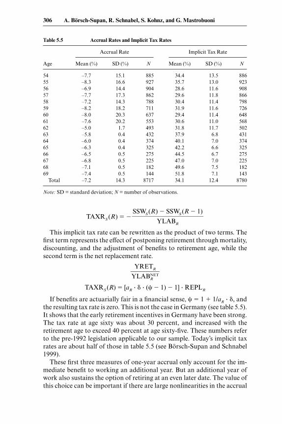
which is displayed in table 5.5. The lack of actuarial fairness of the Germanpublic pension system creates a negative accrual of pension wealth be-tween 5 and 8 percent during the early retirement window when retirementis postponed by one year. The average loss in our sample is about DM10,000 (roughly US$5,000 at purchasing power parity).

A negative accrual can be interpreted as a tax on further labor force par-ticipation. We therefore compute as an implicit tax rate the ratio of the(negative) SSW accrual to the gross wage (YLAB) that workers would earnif they postponed retirement to age R.

SSWS (R ) � SSWS (R � 1)��

SSWS (R � 1)


Table 5.4 Social Security Wealth and Its Accrual

SSW Accrual

Age Mean SD N Mean SD N

54 167.209 82.603 913 –10.084 5.083 91355 169.280 80.628 948 –10.494 5.175 94856 166.391 80.242 930 –8.327 4.356 93057 168.211 80.550 885 –8.730 4.651 88558 171.161 81.672 812 –8.991 4.612 81259 170.002 81.828 736 –9.360 4.713 73660 172.426 80.792 656 –8.565 4.565 65661 175.892 81.324 572 –8.929 4.690 57262 182.616 77.848 507 –9.064 4.780 50763 191.603 75.784 434 –10.997 4.302 43464 194.370 76.811 375 –11.643 4.512 37565 194.654 76.697 325 –12.149 4.652 32566 197.866 76.820 275 –12.855 4.846 27567 197.180 76.052 225 –13.374 5.038 22568 196.372 77.633 182 –13.869 5.330 18269 196.469 78.187 144 –14.424 5.637 144

Total 175.948 80.691 8919 –9.908 4.995 8919

Note: All figures in € 1995 (€1 has a purchasing power of about US$1.00) SD = standard de-viation; N = number of observations.

TAXRS (R) � �

This implicit tax rate can be rewritten as the product of two terms. Thefirst term represents the effect of postponing retirement through mortality,discounting, and the adjustment of benefits to retirement age, while thesecond term is the net replacement rate.

�Y

Y

L

R

A

E

B

T

RN

R

ET�

TAXRS (R) � [aR � � � (� � 1) � 1] � REPLR

If benefits are actuarially fair in a financial sense, � � 1 � 1/aR � �, andthe resulting tax rate is zero. This is not the case in Germany (see table 5.5).It shows that the early retirement incentives in Germany have been strong.The tax rate at age sixty was about 30 percent, and increased with theretirement age to exceed 40 percent at age sixty-five. These numbers referto the pre-1992 legislation applicable to our sample. Today’s implicit taxrates are about half of those in table 5.5 (see Börsch-Supan and Schnabel1999).

These first three measures of one-year accrual only account for the im-mediate benefit to working an additional year. But an additional year ofwork also sustains the option of retiring at an even later date. The value ofthis choice can be important if there are large nonlinearities in the accrual

SSWS (R) � SSWS (R � 1)��

YLABR


Table 5.5 Accrual Rates and Implicit Tax Rates

Accrual Rate Implicit Tax Rate

Age Mean (%) SD (%) N Mean (%) SD (%) N

54 –7.7 15.1 885 34.4 13.5 88655 –8.3 16.6 927 35.7 13.0 92356 –6.9 14.4 904 28.6 11.6 90857 –7.7 17.3 862 29.6 11.8 86658 –7.2 14.3 788 30.4 11.4 79859 –8.2 18.2 711 31.9 11.6 72660 –8.0 20.3 637 29.4 11.4 64861 –7.6 20.2 553 30.6 11.0 56862 –5.0 1.7 493 31.8 11.7 50263 –5.8 0.4 432 37.9 6.8 43164 –6.0 0.4 374 40.1 7.0 37465 –6.3 0.4 325 42.2 6.6 32566 –6.5 0.5 275 44.5 6.7 27567 –6.8 0.5 225 47.0 7.0 22568 –7.1 0.5 182 49.6 7.5 18269 –7.4 0.5 144 51.8 7.1 143

Total –7.2 14.3 8717 34.1 12.4 8780

Note: SD = standard deviation; N = number of observations.

profile. For example, if there is a small negative accrual at age fifty-nine, buta large positive accrual at age sixty, it would be misleading to say that thesystem induces retirement at age fifty-nine; the disincentive to work at thatage is dominated by incentives to work at age sixty.

One way of capturing this possibility is to use the “peak value” calcula-tion suggested by Coile and Gruber (1999). Rather than taking the differ-ence between SSW today and next year, peak value takes the difference be-tween SSW today and in the year in which the expected value of SSW ismaximized:

PEAKVALS (R) � SSWS (R) � maxT R

[SSWS(T )].

This measure therefore captures the tradeoff between retiring today andworking until a year with a much higher SSW. In years beyond the year inwhich SSW peaks, this calculation collapses to the simple one-year accrualvariable. In fact, PEAKVAL turns out to be virtually identical to AC-CRUAL since pension accrual is negative in most cases for the whole se-quence of retirement ages (see the averages in table 5.6).

All these measures include the financial aspects of the retirement deci-sion only. Alternatively, one might consider the consumption utility of netearnings and pension benefits and also account for the utility aspects of thelabor-for-leisure trade-off. To this end, we employ as the fifth and final in-centive variable the option value to postpone retirement (Stock and Wise


Table 5.6 Peak Value and Option Value

Peak Value Option Value

Age Mean SD N Mean SD N

54 –10.084 5.085 913 66.414 111.233 91355 –10.493 5.176 948 61.179 101.163 94856 –8.326 4.357 930 59.015 93.312 93057 –8.728 4.652 885 55.770 118.974 88558 –8.986 4.622 812 49.709 115.357 81259 –9.320 4.764 736 42.628 98.487 73660 –8.531 4.612 656 33.888 51.254 65661 –8.904 4.717 572 25.936 44.513 57262 –9.064 4.780 507 15.646 33.281 50763 –10.997 4.302 434 5.900 16.255 43464 –11.643 4.512 375 2.806 12.175 37565 –12.149 4.652 325 0.428 7.975 32566 –12.855 4.846 275 –1.341 6.873 27567 –13.374 5.038 225 –3.188 5.724 22568 –13.869 5.330 182 –4.984 4.855 18269 –14.424 5.637 144 –6.642 4.029 144

Total –9.900 5.007 8919 38.167 87.540 8919

Note: See table 5.4.


Fig. 5.4 Grid search for three estimation variantsSource: Authors’ estimates based on GSOEP panel of males (available at http://www.diw-berlin.de/gsoep). See text for explanation of legend.

1990). This value expresses for each retirement age the trade-off betweenretiring now (resulting in a stream of utility that depends on this retirementage) and keeping all options open for some later retirement date (with as-sociated streams of utility for all possible later retirement ages).

Let Vt(R) denote the expected discounted future utility at age t if theworker retires at age R, specified as follows:

Vt (R) � ∑R�1

s�t

u (YLABsNET) � as � �s�t � ∑

�

s�R

u(YRETs (R)) � as� �s�t.

YLABsNET � after-tax labor income at age s, s � t . . . R – 1

YRETs (R) � pension income at age s, s RR � retirement age � marginal utility of leisure (to be estimated)a � probability to survive at least until age s� � discount factor � 1/(1� r)

Utility from consumption is represented by an isoelastic utility functionin after-tax income, u(Y ) � Y �. (Remember that pension income in Ger-many is effectively untaxed.) To capture utility from leisure, utility duringretirement is weighted by 1, where 1/ is the marginal disutility of work.

We employed a grid search for the parameter , applied to three specifi-cations (see figure 5.4). The parameter gets smaller as more covariates areused: It is larger than 4 if only a second-order age polynomial is included(plus option value), 2.8 if initial SSW is added, and 2.5 if a large set of re-gressors including a full set of age dummies is added (see table 5.7).

The option value for a specific age is defined as the difference betweenthe maximum attainable consumption utility of the worker postpones re-tirement to some later year minus the utility of consumption that theworker can afford if the worker would retire now. Let R∗(t) denote the op-timal retirement age if the worker postpones retirement past age t, thatis, max(Vt (r)) for r t. With this notation, the option value is

G(t) � Vt (R∗(t)) � Vt (t).

Since a worker is likely to retire as soon as the utility of the option topostpone retirement becomes smaller than the utility of retiring now, re-tirement probabilities should depend negatively on the option value.

The option value captures the economic incentives created by thepension system and the labor market because the retirement incomeYRETs(R) depends on retirement age according to the adjustment factorsand on previous labor income by the benefit rules summarized in sections5.2 and 5.3. The option value is also closely linked to the pension accrual.This is most easily seen in a simple two-period comparison and for � equals1. In this crude approximation, a worker of age R in the first period will re-tire early if

� W(R) YLABNET � �W(R � 1),

where W(t) denotes the present discounted value of pension benefits whenretiring at age t. Using the definition of TAXR(R), it follows that a workerwill retire in the first period if TAXR(R) 1/. Hence, according to thiscrude approximation, the tax rates well above 50 percent exerted by thecurrent public pension system in Germany will lead to early retirement.

We compute the option value for every person in our sample, using theapplicable pension regulations and the imputed earning histories. The pa-rameters chosen are a discount rate � of 3 percent, a curvature parameter


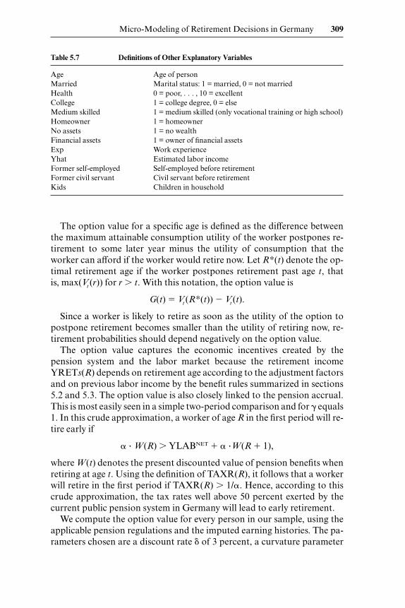
Table 5.7 Definitions of Other Explanatory Variables

Age Age of personMarried Marital status: 1 = married, 0 = not marriedHealth 0 = poor, . . . , 10 = excellentCollege 1 = college degree, 0 = elseMedium skilled 1 = medium skilled (only vocational training or high school)Homeowner 1 = homeownerNo assets 1 = no wealthFinancial assets 1 = owner of financial assetsExp Work experienceYhat Estimated labor incomeFormer self-employed Self-employed before retirementFormer civil servant Civil servant before retirementKids Children in household

� of 1.0, and a relative utility parameter of 2.8. Additional private pen-sion income is ignored because it represents only a very small proportionof retirement income as described before. Table 5.6 shows the sample aver-ages.

5.5 Regression Results

The variable to be explained is old-age labor force status. Because Ger-many has very few part-time employees, we model only two states—fullyin the labor force and fully retired—unlike the competing-risk analysis ofSueyoshi (1989). We use definition I for retired, based on the self-assessedlabor force status (see section 5.4.3).

In each of the following regressions, our main explanatory variable isone of the four incentive variables described in the previous section: ac-crual rate, implicit tax rate, peak value (which is essentially identical to theaccrual of SSW), and option value. The other explanatory variables are theusual suspects: an array of socioeconomic variables, such as gender, mari-tal status, wealth (indicator variables of several financial and real-wealthcategories), and a self-assessed health measure ranging from 0 for poor to10 for excellent health. We do not use the legal disability status as a mea-sure of health since this is endogenous to the retirement decision. The de-sire for early retirement may prompt workers to seek disability status, andfrequently the employer helps in this process to alleviate restructuring. Un-til recently, disability status was granted for labor market reasons withouta link to health.

We link the explanatory variables to the dependent variable by a binaryprobit model. This does some injustice to the panel nature of our data andprobably underestimates the true effect (see Börsch-Supan 2001b, who ex-periments with several specifications of panel probit models with parame-trized correlation patterns over time). This more complicated models can beinterpreted as partly nonparametric hazard models for multiple spell data,permitting unobserved heterogeneity and state dependence without impos-ing a functional form on the duration in a given state, while the simple pro-bit model ignores these temporal effects.22 We conducted several random-effect estimates that correct for some of the intertemporal correlations. Theeffects of the incentive variables were slightly strengthened, but the resultsdid not change significantly. Note that our estimation sample includes re-peated observations of the same person only while this person is employed.Once the person retires, we assume that this is an absorbing state and in-clude only the first observation in retirement. Hence, our dependent vari-able is in fact the probability to retire, given that the sample person has


22. Flexible-hazard-rate models of retirement have been estimated by Sueyoshi (1989) andMeghir and Whitehouse (1997), and parametric-hazard-rate models for German data havebeen estimated by Schmidt (1995) and Börsch-Supan and Schmidt (1996).

worked during the year before, pt � Prob(retired in t | worked in t – 1). Wethen compute the survivor function S(t) conditional on working until thebeginning of our window period (age fifty-three) as the product of (1 – pt )from age fifty-three to t. The probability of choosing a retirement age a isthen pa � S(a) and the expected retirement age is Σpa � S(a) � a.

Inserting the option value in this type of a regression model is a practi-cal estimation procedure that can be interpreted as a flexible discrete-timeduration model explaining the timing of retirement entry. It ignores, how-ever, the structure of the dynamic optimization that underlies the workersdecision regarding when to retire.23 Nevertheless, previous experimenta-tion has shown that this pragmatic approach generates robust estimates ofthe average effects of the incentive variables on retirement, although it islikely to fail the individual variation as precisely as the true dynamic opti-mization model.24

Identification of the incentive variables is possible only if we have mean-ingful variation in these variables. Sources of variation are

• The level of SSW reached at the earliest retirement age, mainly gener-ated by variation in labor force histories;

• The upper threshold for the social security contributions, mainly gen-erated by their changes over time and the different earnings levels;

• Differences in the pension rules between single workers and couples;• Widely varying age differences between husband and spouse;• Restricted eligibility of self-employed;• Restricted eligibility of women with less than fifteen years of service;• Differences in the pension formula between private-sector employees

and civil servants;• Differences in the ratio between contribution rates and pension bene-

fits across cohorts (younger cohorts have a substantially lower inter-nal rate of return); and

• Several minor rule changes during our the sample period.

We estimated twenty-four different models: We use four different incen-tive variables as our main regressors (accrual rate, tax rate, option value,and peak value; see section 5.4.6). For each of these incentive variables, werun probit regressions with three age specifications (linear, quadratic, anda full set of age dummies) as well as with and without including SSW. Wepool public and private workers, but have separate regressions for malesand females.

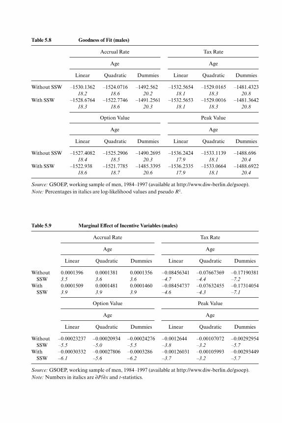
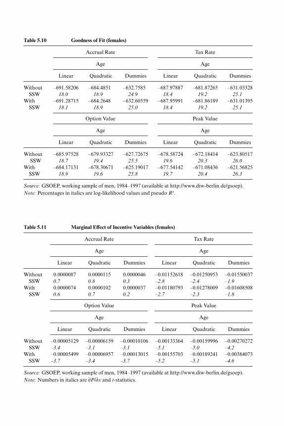
We first summarize our main results separately for men and women.Tables 5.8 and 5.10 report the goodness of fit, and tables 5.9 and 5.11 the im-pact of the incentive variables, measured as the change in the probability of


23. The full underlying dynamic programming model has been estimated by Rust and Phe-lan (1997).

24. See Lumsdaine, Stock, and Wise (1992).

Table 5.9 Marginal Effect of Incentive Variables (males)

Accrual Rate Tax Rate

Age Age

Linear Quadratic Dummies Linear Quadratic Dummies

Without 0.0001396 0.0001381 0.0001356 –0.08456341 –0.07667369 –0.17190381SSW 3.5 3.6 3.6 –4.7 –4.4 –7.2

With 0.0001509 0.0001481 0.0001460 –0.08454737 –0.07632455 –0.17314054SSW 3.9 3.9 3.9 –4.6 –4.3 –7.1

Option Value Peak Value

Age Age


Without –0.00023237 –0.00020934 –0.00024276 –0.0012644 –0.00107072 –0.00292954SSW –5.5 –5.0 –5.5 –3.8 –3.2 –5.7

With –0.00030332 –0.00027806 –0.0003286 –0.00126031 –0.00105993 –0.00293449SSW –6.1 –5.6 –6.2 –3.7 –3.2 –5.7

Source: GSOEP, working sample of men, 1984–1997 (available at http://www.diw-berlin.de/gsoep).Note: Numbers in italics are ∂P/∂x and t-statistics.

Table 5.8 Goodness of Fit (males)


Age Age


Without SSW –1530.1362 –1524.0716 –1492.562 –1532.5654 –1529.0165 –1481.432318.2 18.6 20.2 18.1 18.3 20.8

With SSW –1528.6764 –1522.7746 –1491.2561 –1532.5653 –1529.0016 –1481.364218.3 18.6 20.3 18.1 18.3 20.8


Age Age


Without SSW –1527.4082 –1525.2906 –1490.2695 –1536.2424 –1533.1139 –1488.69618.4 18.5 20.3 17.9 18.1 20.4

With SSW –1522.938 –1521.7785 –1485.3395 –1536.2335 –1533.0664 –1488.692218.6 18.7 20.6 17.9 18.1 20.4

Source: GSOEP, working sample of men, 1984–1997 (available at http://www.diw-berlin.de/gsoep).Note: Percentages in italics are log-likelihood values and pseudo R2.

Table 5.11 Marginal Effect of Incentive Variables (females)


Age Age


Without 0.0000087 0.0000115 0.0000046 –0.01152618 –0.01250953 –0.01550037SSW 0.7 0.8 0.3 –2.8 –2.4 –1.9

With 0.0000074 0.0000102 0.0000037 –0.01180793 –0.01278009 –0.01608508SSW 0.6 0.7 0.2 –2.7 –2.3 –1.8


Age Age


Without –0.00005129 –0.00006159 –0.00010106 –0.00133364 –0.00159996 –0.00270272SSW –3.4 –3.1 –3.1 –5.1 –5.0 –4.2

With –0.00005499 –0.00006957 –0.00013015 –0.00155703 –0.00189241 –0.00384073SSW –3.7 –3.4 –3.7 –5.2 –5.1 –4.6

Source: GSOEP, working sample of men, 1984–1997 (available at http://www.diw-berlin.de/gsoep).Note: Numbers in italics are ∂P/∂x and t-statistics.

Table 5.10 Goodness of Fit (females)


Age Age


Without –691.58206 –684.4851 –632.7585 –687.97887 –681.87265 –631.03328SSW 18.0 18.9 24.9 18.4 19.2 25.1

With –691.28715 –684.2648 –632.60559 –687.95991 –681.86189 –631.01395SSW 18.1 18.9 25.0 18.4 19.2 25.1


Age Age


Without –685.97528 –679.93327 –627.72675 –678.58724 –672.18414 –623.80517SSW 18.7 19.4 25.5 19.6 20.3 26.0

With –684.17131 –678.30671 –625.19017 –677.54142 –671.08436 –621.56825SSW 18.9 19.6 25.8 19.7 20.4 26.3

Source: GSOEP, working sample of men, 1984–1997 (available at http://www.diw-berlin.de/gsoep).Note: Percentages in italics are log-likelihood values and pseudo R2.

being retired when the incentive variable is changed infinitesimally. Tables5.12 and 5.13 show full regression results for our favorite specification (op-tion value with SSW and with a full set of age dummies). The other specifi-cations produce very similar results in terms of significance and signs.

Using tax rate and peak value yield significantly better fits than accrualrate and option value in almost all specifications. There is little difference


Table 5.12 Probit Estimates for Male Subsample—Incentive Variable OV

dF /dx SE z P z x-bar 95% C.I.

OPTVAL –.003053 .0000485 –6.07 0.000 249.725 –.0004 –.00021FSSW –.0001714 .0000361 –4.67 0.000 316.764 –.000242 –.000101AGEDUM55* –.0035989 .0146005 –0.24 0.810 .137001 –.032215 .025018AGEDUM56* .0171014 .0172827 1.09 0.275 .133765 –.016772 .050975AGEDUM57* .0283252 .0191398 1.72 0.086 .123902 –.009188 .065838AGEDUM58* .03864 .0213393 2.20 0.028 .111111 –.003184 .080464AGEDUM59* .0422839 .0230766 2.26 0.024 .096933 –.002945 .087513AGEDUM60* .1134217 .0357241 4.60 0.000 .081368 .043404 .18344AGEDUM61* .1363814 .0140872 4.97 0.000 .062567 .055852 .216911AGEDUM62* .112833 .0408826 4.05 0.000 .045307 .032704 .192961AGEDUM63* .1994108 .0552118 5.69 0.000 .033595 .091198 .307624AGEDUM64* .4444502 .0744151 8.93 0.000 .022346 .298599 .590301AGEDUM65* .3689588 .0861118 6.71 0.000 .01125 .200183 .537735AGEDUM66* .7122481 .084577 8.69 0.000 .006164 .540834 .883662AGEDUM67* .4784933 .2128542 3.34 0.001 .001079 .061307 .89568AGEDUM68* .3776805 .2945118 2.03 0.042 .00616 –.199552 .954913AGEDUM71* .6680958 .3101597 2.53 0.012 .000308 .060194 1.276HEALTH –.0101493 .0009479 –11.65 0.000 9.07096 –.012007 –.008292MARRIED* –.0076327 .0119856 –0.68 0.498 .95161 –.031124 .015859UNI* –.027545 .007122 –2.96 0.003 .128833 –.041504 –.013586SKILL .0029414 .0058029 0.51 0.612 .869934 –.008432 .014315VEIGEN* .0062658 .0050534 1.24 0.216 .53059 –.003639 .01617VNULL* –.0050004 .0078429 –0.61 0.541 .087225 –.020372 .010371VWP* .0156084 .0067196 2.51 0.012 .229619 .002438 .028779VPDAUER .0001696 .001485 0.11 0.909 38.3005 –.002741 .00308VPDAUER2 –3.57e-06 .0000249 –0.14 0.886 1521.28 –.000052 .000045YHAT .0012985 .0003284 3.92 0.000 59.9149 .000655 .001942YHAT2 2.80e-06 5.51e-07 4.95 0.000 4499.21 1.7e-06 3.9e-06ds* –.022587 .0057826 –3.13 0.002 .107104 –.033921 –.011253db* .0464132 .0141686 4.14 0.000 .093389 .018643 .074183KIDS* –.0075237 .0048206 –1.55 0.122 .419171 –.016972 .001925

Obs. P .0826013Pred. P .0412237 (at x-bar)No. of obs. = 6,489LR �2 (31) = 870.62Prob �2 = 0.0000Pseudo R2 = 0.2353Log-likelihood = –1414.5558

Source: GSOEP, working sample of men, 1984–1997 (available at http://www.diw-berlin.de/gsoep).Note: An asterisk denotes dummy variables.

between including SSW or not, although introducing age dummies makesa large difference. Judging from the goodness of fit, the regression with agedummies but without SSW, is our favorite specification. The pseudo R2 isjust about 20 percent, a satisfactory but not excellent value.

All incentive variables have the correct sign and are highly significant.


Table 5.13 Probit Estimates for Female Subsample—Incentive Variable OV

dF /dx SE z P z x-bar 95% C.I.

OPTVAL –.0001008 .0000657 –3.54 0.000 157.169 –.000229 .000028FSSW –.0000474 .0000351 –2.13 0.033 118.39 –.000116 .000021AGEDUM55* –.000499 .0044412 –0.11 0.912 .152008 –.009204 .008206AGEDUM56* .0009751 .0049257 0.21 0.835 .137986 –.008679 .010629AGEDUM57* –.0006681 .0043968 –0.15 0.882 .12747 –.009286 .00795AGEDUM58* .0002302 .0047638 0.05 0.961 .114404 –.009107 .009567AGEDUM59* .0042321 .0073449 0.78 0.434 .100064 –.010164 .018628AGEDUM60* .0606805 .0448888 4.97 0.000 .079987 –.0273 .148661AGEDUM61* .1375386 .0839864 6.78 0.000 .051307 –.027072 .302149AGEDUM62* .0385825 .0360184 2.92 0.003 .028043 –.032012 .109177AGEDUM63* .0209055 .0247693 1.79 0.074 .02167 –.027641 .069241AGEDUM64* .0712695 .0611771 3.48 0.001 .015296 –.048636 .191174AGEDUM65* .2828068 .1450685 6.64 0.000 .011791 –.001522 .567136AGEDUM66* .4289469 .2050834 5.55 0.000 .004461 .026991 .830903AGEDUM67* .0305762 .0538137 1.08 0.279 .002231 –.074897 .136049AGEDUM69* –.0046263 .0085027 –0.40 0.691 .001912 –.021291 .012039AGEDUM70* .010992 .0402127 0.40 0.690 .000956 –.067823 .089808AGEDUM71* .017278 .0628126 0.44 0.662 .000637 –.105832 .140388HEALTH –.0018635 .001441 –4.52 0.000 9.42065 –.004688 .000961MARRIED* –.028244 .0195633 –4.46 0.000 .950605 –.066587 .010099UNI* –.0063273 .0056794 –1.53 0.126 .035692 –.017459 .004804SKILL –.005533 .004353 –2.82 0.005 .476099 –.014065 .002999VEIGEN* –.0005057 .0019191 –0.27 0.786 .515934 –.004267 .003256VNULL* –.0016109 .0028384 –0.58 0.561 .108987 –.007174 .003952VWP* .0013406 .0026261 0.56 0.575 .202996 –.003806 .006488VPDAUER .0001974 .0003477 0.67 0.504 20.1118 –.000484 .000879VPDAUER2 –3.72e-06 6.74e-06 –0.63 0.529 558.3 –.000017 9.5e-06YHAT .0009701 .0005632 3.97 0.000 28.7974 –.000134 .002074YHAT2 –2.41e-06 6.26e-07 –2.02 0.043 6598 –3.6e-06 –1.2e-06ds* –.006747 .0053123 –2.66 0.008 .089229 –.016887 .003937db* .0410058 .0534307 1.63 0.103 .007967 –.063716 .145728KIDS* .0007423 .0021086 0.36 0.717 .345124 –.00339 .004875

Obs. P .0761632Pred. P .0080778 (at x-bar)No. of obs. = 3,138LR �2 (31) = 462.90Prob �2 = 0.0000Pseudo R2 = 0.2739Log-likelihood = –613.60367

Source: GSOEP, working sample of men, 1984–1997 (available at http://www.diw-berlin.de/gsoep).Note: An asterisk denotes dummy variables.

They are very robust across all the different specifications, including inclu-sion of other covariates, sample selection, and definition of retirement (notshown in table). Including age dummies yields larger marginal effects andbetter precision, while including SSW has a very small weakening effect.

The estimation sample also includes civil servants. We have pro-grammed the incentive variables for civil servants using the pension rulesfor civil servants, which should lead to stronger incentives for early retire-ment. However, estimates for a sample of civil servants only are disap-pointing. The most probable reason is that we do not capture the incentivescreated by promotion possibilities, the main reason for civil servants to re-tire later than measured by our incentive variables.

Turning to the female sample, results are much weaker than for males.While the overall fit is comparable and sometimes even better, the incentivevariables are very weak. Only option value and peak value are significant,with one incorrect sign for peak value in the specification with SSW andlinear age. Table 5.12 shows the full regression results for our favorite spec-ification in the full sample.

The incentive variable (here, option value) is highly significant aspointed out before. The set of age dummies is also highly significant andelevates the probabilities to retire after ages sixty, sixty-three, and sixty-five, the earliest retirement ages under the various pathways (see table 5.1).There clearly is an independent effect of age and the incentive variable onretirement. Self-reported health is also highly significant: Healthier work-ers retire substantially later than those males who report poor health. Mar-ried males do not have a different retirement behavior than single males.However, if there is (still) a child in the household retirement is more likelyto be deferred. The effect of a college degree on retirement age is verystrong and is present although we have an income measure (yhat and yhat2)as an additional control. The wealth variables indicate that there is awealth effect, also weak and barely significant: Persons with higher wealth(indicated by homeownership and financial assets) can afford an earlier re-tirement. Also, higher labor income weakens labor force attachment. Notethat the higher opportunity costs of retirement have already been ac-counted for in the option value variable, and hence, this income effect isover and above this plus the wealth effect. Two dummy variables indicatethe former labor force status. These variables take the value of 1 if the per-son is actually or used to be a self-employed or a civil servant. The modelindicates that the self-employed tend to work longer, while civil servants re-tire earlier. Both result confirm our expectations.

The peaks of the age dummies are now much more pronounced at agesixty and sixty-five, in accordance with the different rules for women. Mostsocioeconomic variables have similar (but weaker) effects compared withthe male sample. Different, however, is the effect of being married: Marriedwomen retire later, probably because they have raised children and there-


fore have an interrupted earnings record such that they are not yet eligiblefor retirement at age sixty.

5.6 Simulation Results

We now apply the estimated coefficients to several simulation experi-ments. We first simulate reforms that are close to what happened in Ger-many in the 1992 reform and what the next reform step may strengthen:shifting the retirement age up by making the system more actuarially fair.Second, we simulate several reforms not specific to Germany and unlikelyto happen, but which are used to compare the retirement incentive effectsacross the countries represented in this volume.

5.6.1 Reform Options Specific to Germany

The first country-specific experiment shows what is likely to happenwhen the 1992 reform is fully phased in. The experiment applies the ad-justment factors for early retirement that have been introduced by the pen-sion reform 1992 (3.6 percent per year of early retirement) and comparesit to the previous situation without any explicit adjustments. The 1992 ad-justment factors have been phased in after our sample period and will takefull force from the year 2004 onward. They are not actuarial fair, and theyare not effective before age sixty because they are overruled by the specialearnings-point credits given under disability insurance.

The second country-specific experiment goes one step further and in-troduces a geometric adjustment of 6 percent per year that comes closer toa actuarially fair adjustment. The experiment can therefore be thought ofas a preview of a potential pension reform after the 2002 elections. It isapplied to all ages in the window period (ages fifty-four to sixty-nine), an-chored at the pivotal retirement age of sixty-five.

For each policy scenario we use the estimated parameter values in orderto compute the probability to retire at age x given that the worker hasworked until age fifty-three. We first display the baseline probabilities (i.e.,predicted under the pension rules of 1972 valid in our sample period). Wethen predicted probabilities under the hypothetical new rules (see figures5.5 and 5.6 based on a specification with age and age squared, rather thanlinear age or a set of age dummies). The figures show the shift to the rightof the distribution, resulting in an increase of the average retirement age.

This resulting increase in retirement age is displayed in table 5.14. Itamounts to eight months for the 1992 reform, and seventeen months for asystem that is almost actuarially fair. Given that the average retirement ageis about sixty years in 1999 for German males, the adjustment factor of 6percent would imply an increase of the retirement age to sixty-one-and-one-half years for males. The impact of such a reform on the budget of thePAYG system would be considerable. Given that the average duration of


pension receipts was sixteen years prior to the reform, expenditure woulddecrease by roughly 10 percent through this effect. A second effect worksthrough the extended working life, which leads to higher contributions.Two additional years, relative to forty service years, increase the contribu-tions to the PAYG system by 5 percent—provided that deferred take-up of


Fig. 5.5 Baseline and predicted distribution of retirement ages (1992 reform)Source: GSOEP, working sample of males, 1984–1997 (available at http://www.diw-berlin.de/gsoep).

Fig. 5.6 Baseline and predicted distribution of retirement ages (fair system)Source: GSOEP, working sample of males, 1984–1997 (available at http://www.diw-berlin.de/gsoep).

pensions implies additional employment. Moreover, there is a third bud-getary effect (compared to the no-reform case) since pension benefits arenow lower for all who retire early. This would save another 18 percent.

5.6.2 Simulations for Cross-National Comparisons

This second set of simulations serves as a vehicle for an extensive cross-national comparison of the effects that the early retirement incentives ex-ert on retirement behavior. We use two hypothetical reform scenarios (the“three-year-shift reform” and the “common reform,” later explained inmore detail) and apply them systematically to several variants of our esti-mated models of retirement. These variants include the option value andthe peak value model, each of which is estimated using a linear and adummy-variable age specification. In the latter case and in combinationwith the three-year-shift reform, we introduce yet another two variants:one for keeping the dummy variables at their original ages and one for shift-ing them along with the shift in the incentive variables. These latter variantsare designed to bracket possible behavioral effects that are embedded in the


Table 5.14 Effects of Policy Reforms on Expected Retirement Age

With SSW Without SSW

Age Age


Simulation A (1992 Reform), MenAccrual rate –0.10 –0.10 –0.09 0.41 0.34 0.72Tax rate –0.12 –0.12 –0.11 0.41 0.34 0.73Option value 1.90 1.74 1.55 0.39 0.32 0.73Peak value 2.31 2.16 1.86 0.39 0.31 0.73

Simulation B (6% Geometric Adjustment Factors), MenAccrual rate –0.10 –0.10 –0.09 0.91 0.79 1.57Tax rate –0.12 –0.12 –0.11 0.91 0.79 1.58Option value 2.63 2.45 2.12 1.11 0.93 1.85Peak value 3.06 2.91 2.39 1.11 0.93 1.85

Simulation A (1992 Reform), WomenAccrual rate –0.02 –0.02 –0.01 0.12 0.08 0.08Tax rate –0.02 –0.02 0.00 0.12 0.08 0.09Option value 1.01 0.89 0.77 0.42 0.26 0.40Peak value 1.42 1.28 1.18 0.46 0.27 0.52

Simulation B (6% Geometric Adjustment Factors), WomenAccrual rate –0.02 –0.02 –0.01 0.33 0.25 0.19Tax rate –0.02 –0.02 0.00 0.34 0.26 0.20Option value 1.48 1.32 1.14 1.32 1.05 1.13Peak value 1.98 1.80 1.62 1.41 1.10 1.36

Source: GSOEP, working sample of men, 1984–1997 (available at http://www.diw-berlin.de/gsoep).

age dummies; for a particular example, the habitual effects associated withage sixty-five as a psychological anchor for retirement decisions.

The three-year-shift reform increases the ages of early and normal re-tirement by three years (and the corresponding adjustment factors, if ap-plicable) from the current age in the countries represented by this study.The common reform changes all national systems to a common systemwith an early retirement age of sixty years, a normal retirement age ofsixty-five years, a 60 percent replacement rate at age sixty-five, and a 6 per-cent per year actuarial adjustment, pivoted at age sixty-five.

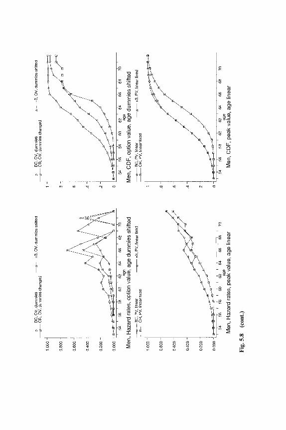
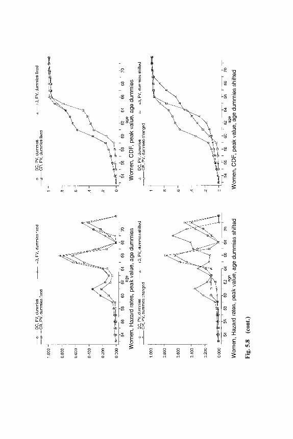
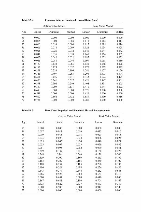
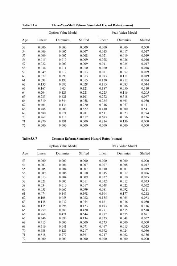
In the following set of figures, we show all our results both in terms ofhazard rates (left-side panels) and the cumulative distribution function (in-verse survival function, right-side panels). For convenience, the hazardrates are also tabulated in the appendix. We summarize our results in table5.15 which displays the expected average retirement ages for all simulations.

Figure 5.7 shows the fit of the option versus the peak value model used


Table 5.15 Expected Retirement Age

Men Women

SampleSample frequencies 61.77 61.89

Base SimulationOption value model

Linear age 62.01 62.02Dummies 61.79 61.89

Peak value modelLinear age 62.01 62.02Dummies 61.79 61.90

Three-Year-Shift SimulationOption value model

Linear age 63.52 64.50Dummies fixed 63.55 64.21Dummies shifted 65.52 66.23

Peak value modelLinear age 62.65 62.34Dummies fixed 62.46 62.55Dummies shifted 65.04 65.16

Common Reform SimulationOption value model

Linear age 64.31 62.64Dummies fixed 64.17 62.60Dummies changed 63.55 64.21

Peak value modelLinear age 63.56 62.32Dummies fixed 63.30 62.51Dummies changed 62.46 62.55

Note: Expected value is taken over distribution truncated at age 69.

Fig

. 5.7

Fit

of b

ase

case

Fig

. 5.7

(con

t.)

in these simulations. With a linear age specification, the peak value modelslightly underestimates retirement at age sixty-five, but in the other ages thetwo models are very close. They deliver, of course, identical simulationswith a full set of dummy variables for each age since in this case the modelis fully saturated. Table 5.15 shows the variation among the four models interms of expected retirement age and how closely the match the actual re-tirement age.

Figure 5.8 summarizes all simulations. Focusing on the cumulative re-tirement function, the three-year-shift reform is much more incisive forGerman men than the common reform, since the common reform keepsthe current early retirement age as well as the normal retirement age un-changed. The common reform lowers the replacement rate from currentlyaround 70 percent by 10 percentage points. This actually has very littleeffects on retirement age. The shift seen in figure 5.8 is mainly an effect ofchanging the actuarial adjustments and therefore closely corresponds towhat we have seen in simulation B in the previous subsection. The effectsare more complicated for women. Women have an earlier retirement age(sixty rather than sixty-three), so that the common reform has an evenlarger effect on women than on men. However, the early retirement age ap-plies only to women with thirty-five years of service. For women with an in-terrupted work history, the reform has little effect at all because they are re-stricted to enter retirement at age sixty-five anyway.

Figure 5.8 also shows that the option value model generally predictslarger effects than the peak value model. This difference is isolated in fig-ure 5.9. As seen by the hazard rates, the option value model has a moresubtle pattern of peaks than the peak value model, which does not reallycapture the in-between-peak at age sixty-three.

Another eye-catching difference in figure 5.8 stems from the impact ofshifting the dummies as an approximation of the effect, by which all age-specific behavior is shifted by three years. Figure 5.10 isolated these differ-ences for the three-year-shift reform and shows that this makes a hugedifference—by about two years concerning the expected retirement age.While these two years are probably an exaggeration of the long-run impactof a later retirement age, the short-run impact measured by keeping thedummies in place is probably an underestimate.

We finish this paper by summarizing that a reform policy of changing theactuarial adjustments, the early retirement ages, or both can indeed shiftthe retirement age quite substantially. Considering the overall length of re-tirement (which is currently about seventeen years in Germany), the ordersof magnitude—about two years for a set of feasible reform options—isquite significant.


Fig

. 5.8

Bas

e ca

se (B

C),

com

mon

refo

rm (C

R),

and

thre

e-ye

ar-s

hift

(�3)

Fig

. 5.8

(con

t.)

Fig

. 5.8

(con

t.) B

ase

case

(BC

), c

omm

on re

form

(CR

), a

nd th

ree-

year

-shi

ft (�

3)

Fig

. 5.8

(con

t.)

Fig

. 5.8

(con

t.) B

ase

case

(BC

), c

omm

on re

form

(CR

), a

nd th

ree-

year

-shi

ft (�

3)

Fig

. 5.8

(con

t.)

Fig

. 5.9

Opt

ion

valu

e ve

rsus

pea

k va

lue:

Sim

ulat

ions

Fig

. 5.9

(con

t.)

Fig

. 5.9

(con

t.) O

ptio

n va

lue

vers

us p

eak

valu

e: S

imul

atio

ns

Fig

. 5.9

(con

t.)

Fig

. 5.9

(con

t.) O

ptio

n va

lue

vers

us p

eak

valu

e: S

imul

atio

ns

Fig

. 5.9

(con

t.)

Fig

. 5.1

0S

imul

atio

ns w

ith

fixed

ver

sus

shif

ted

dum

mie

s

Fig

. 5.1

0(c

ont.

)


Appendix

Table 5A.1 Sample Hazard Rates

Men Women

95% 95% 95% 95%Lower Upper Lower Upper

Age N Mean SD Bound Bound N Mean SD Bound Bound

54 861 0.013 0.004 0.005 0.020 470 0.017 0.006 0.005 0.02955 889 0.015 0.004 0.007 0.023 477 0.019 0.006 0.007 0.03156 868 0.026 0.005 0.016 0.037 433 0.025 0.008 0.011 0.04057 804 0.041 0.007 0.027 0.055 400 0.025 0.008 0.010 0.04058 721 0.060 0.009 0.042 0.077 359 0.033 0.009 0.015 0.05259 629 0.073 0.010 0.053 0.094 314 0.051 0.012 0.026 0.07560 528 0.155 0.016 0.124 0.186 251 0.219 0.026 0.168 0.27161 406 0.185 0.019 0.147 0.223 161 0.348 0.038 0.273 0.42262 294 0.146 0.021 0.106 0.187 88 0.159 0.039 0.081 0.23763 218 0.225 0.028 0.169 0.281 68 0.103 0.037 0.029 0.17764 145 0.428 0.041 0.346 0.509 48 0.188 0.057 0.073 0.30265 73 0.315 0.055 0.206 0.424 37 0.486 0.083 0.318 0.65566 40 0.700 0.073 0.552 0.848 14 0.643 0.133 0.356 0.93067 7 0.429 0.202 –0.066 0.923 7 0.286 0.184 –0.166 0.73768 4 0.250 0.250 –0.546 1.046 5 0.000 0.000 0.000 0.00069 4 0.000 0.000 0.000 0.000 6 0.167 0.167 –0.262 0.59570 3 0.000 0.000 0.000 0.000 3 0.333 0.333 –1.101 1.76871 2 0.500 0.500 –5.853 6.853 2 0.500 0.500 –5.853 6.85372 1 0.000 • • • 0 • • • •73 2 0.000 0.000 0.000 0.000 0 • • • •74 1 0.000 • • • 0 • • • •75 0 • • • • 0 • • • •

Note: N = number of observations; SD = standard deviation. Dots indicate observations.

Table 5A.2 Base Case: Empirical and Simulated Hazard Rates (men)

Option Value Model Peak Value Model

Age Sample Linear Dummies Linear Dummies

53 0.000 0.000 0.000 0.000 0.00054 0.013 0.007 0.012 0.009 0.01255 0.015 0.013 0.014 0.016 0.01456 0.026 0.023 0.027 0.024 0.02657 0.041 0.039 0.041 0.039 0.04158 0.060 0.064 0.059 0.059 0.05959 0.073 0.100 0.076 0.088 0.07560 0.155 0.141 0.156 0.136 0.15661 0.185 0.182 0.181 0.181 0.18262 0.146 0.211 0.145 0.218 0.14563 0.225 0.258 0.225 0.285 0.25564 0.428 0.289 0.427 0.323 0.42665 0.315 0.310 0.316 0.280 0.32666 0.700 0.412 0.698 0.356 0.69267 0.429 0.424 0.425 0.437 0.42668 0.250 0.379 0.239 0.447 0.23469 0.000 0.507 0.000 0.537 0.00070 0.000 0.472 0.000 0.540 0.00071 0.500 0.550 0.500 0.623 0.50072 0.000 0.671 0.000 0.717 0.000

Table 5A.3 Three-Year-Shift Reform: Simulated Hazard Rates (men)


Age Linear Dummies Shifted Linear Dummies Shifted

53 0.000 0.000 0.000 0.000 0.000 0.00054 0.003 0.004 0.004 0.010 0.013 0.01355 0.005 0.004 0.005 0.016 0.014 0.01456 0.008 0.009 0.006 0.024 0.028 0.01257 0.013 0.012 0.006 0.039 0.042 0.01458 0.023 0.018 0.008 0.059 0.059 0.01559 0.036 0.022 0.015 0.087 0.073 0.03560 0.050 0.046 0.017 0.107 0.080 0.03461 0.077 0.065 0.025 0.146 0.096 0.04962 0.097 0.052 0.025 0.179 0.072 0.05163 0.142 0.106 0.065 0.237 0.120 0.08864 0.179 0.265 0.074 0.284 0.304 0.09465 0.222 0.211 0.065 0.328 0.475 0.07566 0.274 0.517 0.112 0.400 0.805 0.11767 0.265 0.240 0.224 0.351 0.203 0.18768 0.252 0.131 0.129 0.363 0.092 0.31369 0.387 0.000 0.482 0.465 0.000 0.67470 0.364 0.000 0.196 0.455 0.000 0.14971 0.493 0.432 0.179 0.559 0.316 0.07772 0.617 0.000 0.000 0.649 0.000 0.000

Table 5A.4 Common Reform: Simulated Hazard Rates (men)



53 0.000 0.000 0.000 0.000 0.000 0.00054 0.006 0.009 0.004 0.010 0.014 0.01355 0.010 0.010 0.004 0.017 0.015 0.01456 0.016 0.018 0.009 0.026 0.034 0.02857 0.026 0.026 0.012 0.040 0.047 0.04258 0.041 0.035 0.018 0.060 0.064 0.05959 0.062 0.042 0.022 0.085 0.071 0.07360 0.086 0.088 0.046 0.099 0.068 0.08061 0.137 0.130 0.065 0.139 0.088 0.09662 0.187 0.123 0.052 0.175 0.069 0.07263 0.269 0.238 0.106 0.241 0.127 0.12064 0.341 0.497 0.265 0.293 0.333 0.30465 0.401 0.426 0.211 0.353 0.524 0.47566 0.456 0.741 0.517 0.421 0.847 0.80567 0.398 0.394 0.240 0.404 0.331 0.20368 0.350 0.209 0.131 0.410 0.147 0.09269 0.498 0.000 0.000 0.525 0.000 0.00070 0.539 0.000 0.000 0.626 0.000 0.00071 0.602 0.564 0.432 0.689 0.690 0.31672 0.724 0.000 0.000 0.781 0.000 0.000

Table 5A.5 Base Case: Empirical and Simulated Hazard Rates (women)


Age Sample Linear Dummies Linear Dummies

53 0.000 0.000 0.000 0.000 0.00054 0.017 0.011 0.016 0.013 0.01655 0.019 0.018 0.018 0.021 0.01856 0.025 0.028 0.024 0.026 0.02457 0.025 0.043 0.024 0.040 0.02458 0.033 0.067 0.033 0.059 0.03259 0.051 0.095 0.052 0.079 0.05160 0.219 0.137 0.221 0.150 0.22261 0.348 0.16 0.346 0.179 0.34662 0.159 0.200 0.160 0.215 0.16263 0.103 0.229 0.105 0.250 0.10764 0.188 0.257 0.185 0.280 0.18665 0.486 0.324 0.488 0.256 0.48666 0.643 0.377 0.644 0.262 0.64567 0.286 0.523 0.303 0.561 0.31368 0.000 0.634 0.000 0.640 0.00069 0.167 0.681 0.180 0.704 0.16770 0.333 0.822 0.337 0.873 0.33771 0.500 0.905 0.500 0.942 0.50072 0.000 0.000 0.000 0.000 0.000

Table 5A.6 Three-Year-Shift Reform: Simulated Hazard Rates (women)



53 0.000 0.000 0.000 0.000 0.000 0.00054 0.006 0.007 0.007 0.013 0.017 0.01755 0.009 0.007 0.008 0.021 0.019 0.01956 0.015 0.010 0.009 0.028 0.026 0.01657 0.022 0.009 0.009 0.041 0.025 0.01758 0.034 0.011 0.010 0.060 0.033 0.01859 0.049 0.017 0.013 0.081 0.052 0.02960 0.072 0.099 0.013 0.093 0.111 0.01961 0.098 0.198 0.015 0.120 0.212 0.02462 0.135 0.082 0.028 0.155 0.083 0.04463 0.167 0.05 0.121 0.187 0.050 0.11064 0.204 0.123 0.221 0.225 0.116 0.20565 0.283 0.421 0.101 0.272 0.518 0.06766 0.310 0.544 0.058 0.285 0.691 0.03067 0.401 0.134 0.220 0.346 0.057 0.11168 0.488 0.000 0.622 0.410 0.000 0.54169 0.580 0.071 0.781 0.511 0.023 0.79470 0.762 0.217 0.312 0.683 0.056 0.12671 0.870 0.391 0.000 0.814 0.136 0.00072 0.000 0.000 0.000 0.000 0.000 0.000

Table 5A.7 Common Reform: Simulated Hazard Rates (women)



53 0.000 0.000 0.000 0.000 0.000 0.00054 0.003 0.004 0.007 0.007 0.008 0.01755 0.005 0.004 0.007 0.010 0.007 0.01956 0.009 0.006 0.010 0.015 0.012 0.02657 0.013 0.004 0.009 0.022 0.010 0.02558 0.021 0.005 0.011 0.032 0.012 0.03359 0.034 0.010 0.017 0.048 0.022 0.05260 0.053 0.067 0.099 0.081 0.092 0.11161 0.074 0.145 0.198 0.104 0.177 0.21262 0.108 0.058 0.082 0.135 0.065 0.08363 0.138 0.037 0.054 0.161 0.036 0.05064 0.175 0.096 0.123 0.193 0.086 0.11665 0.259 0.380 0.420 0.271 0.515 0.51866 0.268 0.471 0.544 0.277 0.675 0.69167 0.346 0.090 0.134 0.325 0.048 0.05768 0.415 0.000 0.000 0.375 0.000 0.00069 0.516 0.041 0.071 0.467 0.015 0.02370 0.688 0.126 0.217 0.592 0.024 0.05671 0.818 0.277 0.391 0.717 0.062 0.13672 0.000 0.000 0.000 0.000 0.000 0.000

References

Birg, H., and A. Börsch-Supan. 1999. Für eine neue Aufgabenteilung zwischen geset-ziclicher und privater Altersversorgung (A new division of labor between publicand private pensions). Berlin: GDV.

Börsch-Supan, A. 1992. Population aging, social security design, and early retire-ment. Journal of Institutional and Theoretical Economics 148:533–57.

———. 1995. Regional development, capital flows, and trade policies in an agingEurope. In Neue entwicklungen in der regionalökonomik (New developments inregional economics), ed. B. Gahlen, H. Hesse, and H. J. Ramser, 237–63.

———. 1998. Germany: A social security system on the verge of collapse. In Re-designing social security, ed. H. Siebert, 129–59. Tübingen, Germany: J. C. B.Mohr.

———. 2000a. A model under siege: A case study of the German retirement insur-ance system. The Economic Journal 110 (461): F24–45.

———. 2000b. Data and research on retirement in Germany. Report for the Na-tional Academy of Sciences, Washington, D.C. University of Mannheim, De-partment of Economics. Mimeograph.

———. 2000c. Incentive effects of social security on labour force participation: Ev-idence in Germany and across Europe. Journal of Public Economics 78:25–49.

———. 2001a. Blaupause für eine nachhaltige rentenreform (Blueprint for a sus-tainable pension reform). University of Mannheim, Department of Economics.Mimeograph.

———. 2001b. Incentive effects of social security under an uncertain disability op-tion. In Themes in the economics of aging, ed. D. A. Wise, 281–310. Chicago: Uni-versity of Chicago Press.

Börsch-Supan, A., and P. Schmidt. 1996. Early retirement in East and West Ger-many. In Employment policy in the transition to free enterprise: German integra-tion and its lessons for Europe, London, ed. R. Riphahn, D. Snower, and K. Zim-mermann, 83–102. Heidelberg, Germany: Springer.

———. 1998. Social security and declining labor force participation in Germany.American Economic Review 88 (2): 173–78.

———. 1999. Social security and retirement in Germany. In International social se-curity comparisons, ed. J. Gruber and D. A. Wise, 135–80. Chicago: Universityof Chicago Press.

Bundesministerium für Arbeit und Sozialordnung (BMA). 1997. Statistischestaschenbuch (Statistical handbook). Bonn, Germany: Bundespresseamt.

Burkhauser, R. 1991. An introduction to the German socio-economic panel forEnglish speaking researchers. Syracuse University, Department of Economics.Mimeograph.

Casmir, B. 1989. Staatliche rentenversicherungssysteme im internationalen Vergleich(Public pensions: An international comparison). Frankfurt, Germany: Lang.

Coile, Courtney. 1999. Retirement incentives and couples’ retirement decisions,Ph.D. diss. MIT, Department of Economics.

Coile, Courtney, and Jonathan Gruber. 1999. Social security and retirement. MIT,Department of Economics. Mimeograph.

Gruber, J., and D. A. Wise, eds. 1999. Social security and retirement around theworld. Chicago: University of Chicago Press.

Jacobs, K., M. Kohli, and K. Rein. 1990. Germany: The diversity of pathways. InTime for retirement: Comparative studies of early exit from the labor force, ed.M. Kohli, M. Rein, A. M. Guillemard, and H. van Gunsteren, 181–221. Cam-bridge: Cambridge University Press.


Lumsdaine, R. L., J. H. Stock, and D. A. Wise. 1992. Three models of retirement:Computational complexity versus predictive validity. In Topics in the economicsof aging, ed. D. A. Wise, 16–60. Chicago: University of Chicago Press.

Meghir, C., and E. Whitehouse. 1997. Labour market transitions and retirement ofmen in the UK. Journal of Econometrics 79:327–54.

Riphahn, Regina T. 1995. Disability retirement among German men in the 1980s.Ludwig Maximilians Universität. Münchner WirtschaftswissenschaftlicheBeiträge (Munich Economics Discussion Papers), no. 95-20. München, Ger-many.

Riphahn, Regina T., and P. Schmidt. 1995. Determinanten des ruhestandes: Locktder ruhestand oder drängt der arbeitsmarkt (Determinants of retirement: Is lei-sure pulling or the labor market pushing)? Center for European Economic Re-search (ZEW) Discussion Paper no. 95-10. Mannheim, Germany.

Rust, J. 1990. Behavior of male workers at the end of the life cycle: An empiricalanalysis of states and controls. In Issues in the economics of aging, ed. D. A. Wise,317–79. Chicago: University of Chicago Press.

Rust, J., and C. Phelan. 1997. How Social Security and Medicare affect retirementbehavior in a world of incomplete markets. Econometrica 65 (4): 781–831.

Schmähl, W. 1991. Alterssicherung in der DDR und ihre umgestaltung im zuge desdeutschen einigungsprozesses—einige verteilungspolitische aspekte (Pensionsin the GDR and their changes during reunification—some distributional as-pects). In Sozialpolitik im vereinten Deutschland (Social policy in a unified Ger-many), ed. G. Kleinhenz, 49–95. Berlin: Duncker and Humblot.

Schmidt, P. 1995. Die wahl des rentenalters—Theoretische und empirische analysedes rentenzugangsverhaltens in West- und Ostdeutschland (The choice of retire-ment age—theoretical and empirical analyses of retirement behavior in Westand East Germany). Frankfurt, Germany: Lang.

Schnabel, R. 1998. Rates of return of the German pay-as-you-go pension system.Finanzarchiv N.F. 55 (3): 374–99.

———. 1999. Opting out of social security: Incentives and participation in theGerman public pension system. SFB504-Discussion Paper no. 99-42. Universityof Mannheim, Department of Economics.

Siddiqui, S. 1997. The pension incentive to retire: Empirical evidence for West Ger-many. Journal of Population Economics 10 (4): 463–86.

Stock, J. H., and D. A. Wise. 1990. The pension inducement to retire: An optionvalue analysis. In Issues in the economics of aging, ed. D. A. Wise, 205–30. Chi-cago: University of Chicago Press.

Sueyoshi, G. T. 1989. Social security and the determinants of full and partial re-tirement: A competing risk analysis. NBER Working Paper no. 3113. Cam-bridge, Mass.: National Bureau of Economic Research.

Verband Deutscher Rentenversicherungsträger (VDR). 1999. Die rentenver-sicherung in zeitreihen (German public pensions in time series). Frankfurt amMain, Germany: VDR.


Date post:	02-Feb-2022
Category:	Documents
Upload:	others
View:	3 times
Download:	0 times

Social Security Programs and Retirement around the World ...

Documents