204
Socio-economic Impact of National Highway on Rural Population Asian Institute of Transport Development 2011

Socio-economic Impact of
National Highway on Rural Population
Asian Institute of Transport Development
2011

Socio-economic Impact of
National Highway on Rural Population
© Asian Institute of Transport Development, New Delhi
Published 2003 – Phase I of the study
© Asian Institute of Transport Development, New Delhi
Published 2011 – Phase II of the study
The views expressed in the publication are those of the authors and do not necessarily
reflect the views of the Board of Governors of the Institute or its member countries.
Asian Institute of Transport Development (AITD)
13 Palam Marg, Vasant Vihar
New Delhi-110057 INDIA
Phone: +91-11-26155309
Fax +91-11-26156298
Email: [email protected]
Table of Contents
Acknowledgements i
Abbreviations iii
Executive Summary v
Main Findings and Policy related Lessons xvi
Introduction xviii
Chapter 1: Methodology of Impact Evaluation 1
Chapter 2: Survey Structure and Methodology 25
Chapter 3: Socio-economic Profile of Rural Households 52
Chapter 4: Impact Evaluation at Village Level 83
Chapter 5: Impact Evaluation at Household Level 98
Chapter 6: Status of Rural Access and Mobility 132
Concepts and Definitions 141
References 158

Acknowledgements
This study was carried out under the overall guidance of K. L. Thapar,
Chairman, AITD. The study team included Y. K. Alagh, Dalip S. Swamy,
G. S. Bhalla, Ramprasad Sengupta, Dipankor Coondoo, TCA Srinivasa-Raghavan,
George Mathew, S. Gupta, Bhisma Rout, Anjula Negi, Madhav Raghavan and
S. N. Mathur.
Other experts associated with the study were Alakh Narain Sharma,
M. Neelakantan, TCA Anant, D. P. Gupta, Sat Parkash, Anindita Roy Saha,
Anvita Arora, Kaushik R. Bandyopadhyay, Loknath Acharya and Chetana Chaudhuri.
The baseline and follow-up field surveys were carried out with the help of Institute
for Human Development, Delhi and The Vision Consultancy Services, Lucknow
respectively.
The survey team, among others, included S. K. Khanna, S. Bahl, V. S. Ghai,
Balwant Mehta, R. A. Singh, Ranjit Kumar, Nidhi Mehta, Bharat Singh, Srinivas
Pandey and Sarvadev Chaudhary. The PRA exercises were conducted by Centre for
Management and Social Research, Hyderabad and The Vision Consultancy Services,
Lucknow.
The Institute held wide range of consultations at various stages of the study to
firm up the methodology and discuss the findings. Helpful comments were provided
by Hiten Bhaya, Vijay Kelkar, S. R. Hashim, G. K. Chadha, Sudipto Mundle,
Pradipto Ghosh, Anil Bhandari, Zhi Liu, A. L. Nagar, Andrew Chesher, Alok Bansal,
Jyotsna Jalan, Sheila Bhalla, Amitabh Kundu, Dinesh Mohan, Geetam Tiwari,
B. B. Bhattacharya, V. K. Sharma, Nandan Nawn, D. Dasgupta, Indira Rajaraman,
Rajesh Rohatgi and Brijeshwar Singh.
An interactive and participatory workshop was held before the commencement
of the project. The participants included officials of National Highways Authority of
India, the World Bank, National Sample Survey Organisation, Ministry of Rural
Development, Planning Commission, noted researchers and academicians from
Jawaharlal Nehru University, Delhi School of Economics, Indian Statistical Institute,
National Institute of Public Finance & Policy, Indian Institute of Technology, Sardar
Patel Institute of Economics & Social Research, University College, London and
Socio-economic Impact of 4-laning of National Highway on Rural Population
ii
Asian Institute of Transport Development. The meeting was presided over by
Prof. A. L. Nagar, the well-known academician.
On the completion of the first phase of the project, a seminar was arranged to
discuss the findings of the study. The participants included representatives from
Ministry of Finance, Ministry of Rural Development, Ministry of Road Transport and
Highways, Planning Commission, Jawaharlal Nehru University, Delhi University,
Indian Institute of Technology, Institute of Economic Growth, Central Road Research
Institute, National Sample Survey Organisation, Indian Statistical Institute, School of
Planning and Architecture, World Bank, Asian Development Bank and National
Highways Authority of India.
At the conclusion of the project, a seminar was organised to present the main
findings and policy related recommendations of the study. The participants included
representatives from Ministry of Finance, Ministry of Rural Development, Planning
Commission, Jawaharlal Nehru University, Indian Institute of Technology, Institute
of Economic Growth, Indian Statistical Institute, World Bank, Asian Development
Bank, Infrastructure Development Finance Company, National Institute of Public
Finance and Policy, TERI University, Institute for Human Development and National
Highways Authority of India.
The Institute acknowledges the commitment of the National Highways
Authority of India to upgrade the national highway network in the country. The
empirical studies sponsored by NHAI at the instance of the World Bank reflect their
keenness to understand the role of the highways in improving the well-being of the
rural population.
T. C. Kausar, who also coordinated its designing and production, edited the
report. K. K. Sabu and Lalit Malhotra provided the secretarial assistance.
Abbreviations
AFC : Average Fixed Cost
AIOPL : All-India Official Poverty Line
AVC : Average Variable Cost
BDO : Block Development Officer
BLUE : Best Linear Unbiased Estimator
BPL : Below Poverty Line
CBA : Cost Benefit Analysis
CGE : Computable General Equilibrium (Model)
CPIAL : Consumer Price Index for Agricultural Labour
CPIMR : Consumer Price Index for Middle-range Rural Population
CPIMU : Consumer Price Index for Middle-range Urban Population
CPITR : Consumer Price Indices for Total Rural Population
CPITU : Consumer Price Indices for Total Urban Population
CSO : Central Statistical Organisation
CV : Co-efficient of Variation
DRDA : District Rural Development Agency
EC : Encompassing Communities
FSU : First Stage Unit
GDI : Gender-related Development Index
GDP : Gross Domestic Product
GEM : Gender Empowerment Measure
HDI : Human Development Index
HPI : Human Poverty Index
IAY : Indira Awas Yojna
ICMR : Indian Council of Medical Research
ILO : International Labour Organisation
IRDP : Integrated Rural Development Programme
IWW : Institute for Economic Policy Research (University of Karlsruhe, Germany)
JRY : Jawahar Rozgar Yojna
LRMC : Long Run Marginal Cost
LUTI : Land-Use/Transport Interaction
MGNREGA: Mahatma Gandhi National Rural Employment Guarantee Act
MPCE : Monthly Per Capita Consumption Expenditure
MPCY : Monthly Per Capita Income

Socio-economic Impact of 4-laning of National Highway on Rural Population
iv
MRA : Multivariate Regression Analysis
NAS : National Accounts Statistics
NDC : National Development Council
NH : National Highway
NMT : Non-motorised Transport
NPRT : Non-parametric Regression Technique
NRA : Non-parametric Regression Analysis
NSS : National Sample Survey
NSSO : National Sample Survey Organisation
OAE : Own Account Enterprise
ODA : Overseas Development Administration
OLS : Ordinary Least Square
PCTE : Per Capita Total Expenditure
PCTR : Per Capita Trip Rate
PHC : Primary Health Centre
PL : Poverty Line
PRA : Participatory Rural Appraisal
PSMT : Propensity Score Matching Technique
RTS : Rural Transport Services
RTTS : Rural Travel and Transport Survey
SACTRA : Standing Advisory Committee on Trunk Road Assessment
SC/ST : Scheduled Castes and Scheduled Tribes
SEM : Simultaneous Equation Model
SJSY : Swarna Jayanti Swarozgar Yojna
SW : Social Welfare
TFP : Total Factor Productivity
TRT : Trasporti e Territorio Srl (Milano, Italy)
UTs : Union Territories
VLSS : Vietnam Living Standard Survey
WFPR : Workforce Participation Rate
WPI : Wholesale Price Index
WPR : Worker Population Ratio

Executive Summary and Main Findings
1. India has embarked upon a programme of upgrading of its national highway
network, initially connecting the four metropolises and major maritime ports. This
programme requires massive investments. Side by side, the country also carries a
crushing load of poverty, which is more pronounced in the rural areas. According to
the latest estimates, more than one-third of its rural population lives below the poverty
line.
2. The existing level of understanding of the causal relationship between
transport infrastructure and human ‘well-being’ in general and poverty in particular, is
inadequate. Most of the evidence in this regard is anecdotal and not based on
empirical results. Whilst transport is accepted as an important element in both direct
and indirect intervention for poverty reduction, there has so far been little attempt at
formal accounting of poverty in transport projects.
3. In the literature related to the impact analysis of road-related projects, there
are references to studies of the socio-economic impact of rural roads. But there is
virtually no discussion of the impact of a highway, particularly a major national trunk
route. The role of a major highway has been mainly evaluated in traditional terms of
moving intercity passenger and freight traffic. Its socio-economic impact on the rural
population living in its proximity has never been studied.
4. Over time, perceptions of poverty have also undergone a significant change. It
is no longer just monetary income that determines the poverty levels. There are other
dimensions as well. Poverty is now viewed as a level of deprivation of access to
means of attaining one’s potential as a human being physically and intellectually.
Thus, facilities like water, sanitation, connectivity, and educational and medical
services are also recognised as important indices of human development.
5. Typically, investment projects in the transport sector are evaluated by cost-
benefit analysis (CBA) primarily in terms of efficiency considerations. The method is,
however, not even-handed in all cases. It tends to favour investment in high-return
projects. Besides, there are many items where cost-benefits are not readily
quantifiable and therefore do not get adequately reflected. There are also issues of
market imperfections and externalities not captured in the conventional CBA.
Socio-economic Impact of National Highway on Rural Population
vi
6. The growing concern for poverty alleviation has led to a re-examination of the
adequacy of the existing project evaluation criteria in assessing the distributional
impacts. The socio-economic impact analysis, therefore, aims at assessing the
magnitude and distribution of both direct and indirect effects of a project. Keeping all
this in view, it was decided to undertake an evaluation of the socio-economic impact
of four-laning of a stretch of a national highway being four-laned on the rural
population living in its proximity.
7. For this, a long stretch of national highway (NH2) covering a distance of 995
km between Agra and Dhanbad, falling in the states of Uttar Pradesh, Bihar and
Jharkhand, was selected. The issue of poverty alleviation is more pertinent and
relevant in respect of this stretch because most of the areas contiguous to it have a
high incidence of rural poverty. This has also been confirmed by the census conducted
by the state governments concerned for identifying the rural poor for coverage under
various poverty alleviation programmes.
8. The measurement of the impact of an existing road or that of a road-related
project – be it a new road or widening or upgrading an existing one – is generally
beset with a number of problems. Such problems are specific to this kind of projects,
not normally encountered in most other public investment projects. It is essentially
because a road-related project generally has a number of unique features.
9. Firstly, since the various services of a road together form a public good, by
definition is non excludable and non-rivalrous, identifying the beneficiary/
participating population in a road-related project is not simple. Secondly, the impact
of a road-related project often tends to get confounded by the impact of other
interventions on the outcome variables. Finally, the conceptual and methodological
issues in the impact measurement of a road that already exists or has been improved
(by widening, say) may be somewhat different from those arising in the case of the
impact analysis of a new road.
10. The impact of a road (a new one or an upgraded one) consists of direct or first-
round effects, and indirect or a sum total of all later-round effects. Direct effects are
mostly observed in the form of increased mobility, reduced travel time, etc. The
indirect effects, on the other hand, consist of structural changes in the economy due to
enhanced opportunities which would result from increase in mobility arising from the
development of infrastructure.
Executive Summary
vii
11. An economic-theoretic framework has, therefore, been developed to explain
why and how a road or its improvement is expected to affect the well-being of people
living around it. The model justifies using variables related to mobility and socio-
economic well-being as relevant outcome variables, examining the relationship of
each of these variables with the distance from the highway, and delineating the
influence zone of the project.
12. An important issue in assessing the impact of a road or its expansion is the
identification of the influence zone, i.e., the area on either side of the road to which
the impact is supposed to be limited. Based on considerations of accessibility and
connectivity, this zone has, a priori, been delineated to be the area lying within a
distance of 5 km on either side of the chosen segment of NH2. This means the
distance that can be travelled in less than 30 minutes on a bicycle or in one hour on
foot.
13. The areas lying on both sides of the highway beyond the approach distance of
5 km and within the horizontal distance band of 7 km have been treated as the control
zone. This is on the presumption that the socio-economic benefits decline sharply as
the distance exceeds 5 km. The control zone enables comparison with the influence
zone for the purpose of assessing the net socio-economic impact of the project. This
comparison is done under two situations – before and after the implementation of the
project – so as to isolate the effects of other simultaneous development initiatives or
processes.
14. Typically, benefit analyses comprise two studies of socio-economic conditions
– one based on baseline survey data (collected before the project is launched) and the
other based on re-survey data (collected after the project has been completed). The
partial effects of the project are then assessed by appropriately comparing the results
of these two studies. The current report presents the results based on the baseline and
the re-survey data.
15. The methodology of impact assessment makes use of four
statistical/econometric techniques, viz., correlation analysis, comparison of means,
propensity score matching technique (PSMT)-based single difference analysis (SDA)
and double difference analysis (DDA) and non-parametric regression analysis (NRA).
The conventional regression modelling and the more sophisticated PSMT-double
difference method are not substitutes for each other, but rather serve as

Socio-economic Impact of National Highway on Rural Population
viii
complementary exercises where one seeks to corroborate and improve the results in
the overall framework.
16. The methodology adopted having a strong theoretical underpinning helps to
ensure robust empirical results. Compared to conventional evaluation techniques like
cost-benefit analysis or simulation based on the computable general equilibrium
model, or the econometric technique of simultaneous equations model, this
methodology is considered to be more operational, reliable and far less expensive.
17. The statistical/econometric techniques have been supplemented by
participatory rural appraisal (PRA), which, inter alia, includes reflexive or generic
controls. In reflexive comparisons, the participants themselves provide the control
information by comparing themselves ‘before’ and ‘after’ receiving the intervention.
With generic comparisons, the impact of the intervention on beneficiaries is compared
with established norms about typical changes occurring among the target population.
18. The full impact study of the widening of NH2 requires pre- and post-project
household and village level data in respect of possible outcome variables. The impact
assessment has, therefore, been set up in two stages and relies primarily on survey-
based collection of data and quantitative analysis of such data. The relevant universe
comprises all households living in villages belonging to the defined influence and
control zones of the selected stretches of NH2.
19. The area of this universe comprises seven stretches spanning the three states of
Uttar Pradesh, Bihar, and Jharkhand. The representative stretches have been chosen
on the basis of agro-climatic and other macro features, in particular, the incidence of
poverty. In these selected stretches, 1,697 villages lying in the horizontal distance
band of 0-7 km on both sides of NH2 have been identified. It may be clarified that the
concept of horizontal distance is different from that of approach distance. Thus, the
horizontal distance band of 7 km may include villages whose actual approach distance
may be much higher, extending up to 16 km.
20. The sample design adopted for each of these stretches is a stratified two-stage
one – villages being the first stage and households the second stage. The first stage
sample units have been selected using the probability proportional to size (PPS)
without the replacement technique, and those in the second stage have been selected
by using the circular systematic sampling technique. The sample covers 200 villages
Executive Summary
ix
and 3,200 households both in the baseline and follow-up surveys. However, due to
expected time-related attrition only 3071 households could be covered in the resurvey.
21. In order to generate data on village and household characteristics, as well as
different socio-economic causal factors and outcomes of the developmental
intervention of the highway, extensive schedules were prepared for the primary
baseline survey conducted in 2002-03. The baseline survey was followed up by post-
project survey in 2009-10. The list of variables covers, among others, transport
connectivity; mobility patterns; incidence of poverty; income, employment and
occupation; asset ownership; education and health facilities; and attitudinal response.
22. The temporal changes, as revealed by the baseline and the resurvey data sets,
have been analyzed. The summary profiles provide contextual underpinning for
assessing the socio-economic impact of making the national highway four-lane. Since
the time-gap between the two surveys is seven years and not long, any observed
improvement in indicators may partly be ascribed to the NH2 upgrading. The profiles
also help to see if any positive impact of NH2 upgrading has been progressive,
socially inclusive and spatially even-distributed.
23. The profiles clearly bring out a distinct structural shift in the rural economy in
terms of an increase in non-farm activities, higher workforce participation, an increase
in school enrolment and better literacy levels. There is a noticeable increase in female
participation in the workforce as also the school enrolment of girls. These beneficial
changes help in the empowerment of women, a development of considerable
importance for the country.
24. Mobility levels have also risen across all the income classes in terms of
increases in per capita weekly trip rates as well as trip lengths. This is a clear
indication of improvement in job opportunities and access to markets, schools, and
other services. This is also a sign of increase in the spatial distribution of economic
activities.
25. Economic growth and development have been widespread and largely
inclusive. However, the effects of such development have not been uniform across
time or across economic classes. Although the differences have remained they have
substantially narrowed. With Bihar and Jharkhand showing greater improvement, the
disparities there have considerably reduced.
Socio-economic Impact of National Highway on Rural Population
x
26. The non-poor or not-so-poor have benefitted more than the poorer ones. This
is perhaps typical of the early days of development as better-off persons have better
access to facilities. As time goes by, it can be expected that benefits would become
more even.
27. Human dignity depends to a great extent on education. Labour productivity in
the long run is also a function of the levels of schooling received. Average school
enrolment among children has increased to more than 90 percent. Significantly, the
enrolment level among the poor households has also been high – 86 percent.
Furthermore, Bihar and Jharkhand have shown considerable improvement in this
regard. All these developments have long-term beneficial implications.
28. The overall literacy level has improved across all the stretches, but it is still
somewhat lower than the national average. The interstate and class differences also
persist. For example, for the poor households, literacy is 17 percent less compared to
the non-poor households. However, the female literacy rate among the poor
households has increased at a much faster rate than the non-poor households which is
a welfare improvement.
29. It is now well-established that the individual and social returns from the
women’s education are exceptionally high, especially in the matter of lowering of
fertility and infant and child mortality rates, and improvement in the children’s
educational achievements. There has been a significant rise in school enrolment
among girls even in poor households. In this respect, both Bihar and Jharkhand have
done well.
30. The proportion of working women in the total female population has
registered a manifold increase across all economic classes, with Bihar and Jharkhand
registering higher increase. Generally, the female workforce participation rates are
higher in poor households. This position has undergone a dramatic change. The
women from not-so-poor households are also equally participating in the workforce.
31. The overall sex ratio (number of females per 1,000 males) has remained
unchanged and continues to be lower than the national average. The poor households
have a higher sex ratio than the non-poor households. Arguably, better-off
communities have a stronger gender bias against the female than poor households.
Executive Summary
xi
32. In terms of poverty indicators, the proportion of people living below the
poverty line has declined significantly for all the stretches except Auraiya in Uttar
Pradesh both on an overall basis and headcount basis. For scheduled castes and
scheduled tribes, this proportion has also reduced for all the stretches except at two
places in Uttar Pradesh, viz., Auraiya and Firozabad, both on an overall basis and
headcount basis.
33. The average landholding per household is low at 0.63 hectare, with marginally
higher holdings in Bihar and Jharkhand. There is pronounced disparity in resource
endowments across the economic classes. The average landholding of a poor
household is abysmally low – one-eighth of a hectare in Uttar Pradesh and a quarter
of a hectare in Bihar and Jharkhand. The non-poor households are better off,
particularly in Bihar and Jharkhand with an average landholding of 0.98 hectare.
34. The share of income from agriculture particularly in Bihar and Jharkhand has
increased but the number of households engaged in agricultural activities has gone
down in all the representative stretches. The poor households have a smaller share of
income from agriculture in comparison to the non-poor households. However, in case
of poor households, their share from non-agricultural activities has increased.
35. The rationale of the present study is based on the premise that, ceteris paribus,
access to a highway provides to the population living in its appropriately defined
neighbourhood opportunities that help improve their well-being. To verify this
presumption empirically on the basis of village-level data, the relationship between
selected village-level indicators of socio-economic well-being and the proximity of
villages to NH2 has been examined, using different statistical/econometric techniques.
36. The empirical results firmly confirm that proximity to highway has a positive
relationship with: (i) demographic characteristics (density of population), (ii)
proportion of BPL households (iii) share of motorised transport, (iv) employment in
non-farm activities (proportion of non-agricultural workers in total main workers), (v)
housing conditions (proportion of semi-pucca and pucca houses in the total number of
dwellings), (vi) enrolment of students and also that of girl students, and (vii) price of
land (price of irrigated crop land and residential land).
37. The results of non-parametric regression analysis of the follow-up survey
dataset have confirmed that for most of the chosen indicators, there is a desired shift
Socio-economic Impact of National Highway on Rural Population
xii
of the level of the curve in relation to the baseline NRA curve. More importantly, in
many cases, the gradient of the relationship shows a marked change around a distance
level of 4-5 km, indicating that the effect of the highway on villages located within
this approach distance is qualitatively different from that on villages at greater
distances.
38. The improved job opportunities available in closer proximity to the highway
have a significant influence on the demographic characteristics in terms of higher
density of population in the nearby villages. In particular, the relatively poor tend to
stay closer to the highway because of better job prospects in non-agricultural
activities and ease of commuting. This phenomenon has implications for interpreting
the gradient of change.
39. The basic premise underlying the household-level data analysis, as in the case
of analysis of village-level data, is that proximity to NH2 would help improve a
household’s well-being. An improved road infrastructure, in turn, would further
enhance the well-being of the population. Given that the notion of socio-economic
well-being is essentially multi-dimensional, a wide array of household-level outcome
variables (that are likely to reflect the well-being of the population) have been
analysed to assess if proximity to NH2 leads to significant differences in the level of
these variables and also to explore the nature of relationship these variables may have
with the distance from NH2.
40. The results clearly suggest that proximity to NH2 has a significant relationship
with (i) transport and mobility (per capita trip rate, per capita trip rate for work, per
capita trip rate involving travel on NH2, per capita trip length for trips involving NH2,
per capita travel time for trips involving NH2, travel cost per person km for trips
involving NH2), (ii) extent of income and employment in non-farm activities (share
of income from self-employment in non-agricultural activities, female labour
participation, proportion of non-agricultural workers in total working household
members), (iii) asset holding (whether a household owns at least one information
related consumer durable), and (iv) health attainment (proportion of household
members who availed of medical facilities during the last six months).
41. Proximity to NH2 and its upgrading has significant beneficial influence on
many aspects of household well-being especially those relating to mobility and non-
Executive Summary
xiii
agricultural employment, thereby signalling significant structural changes in the local
economies of the neighbourhood of the highway.
42. The beneficial influence systematically declines as the distance from the
highway increases, thus empirically supporting the gradient change hypothesis. The
influence zone generally extends up to a distance of 4-5 km on either side of the
highway. There are, however, some evidences of the expansion of the influence zone
beyond this distance slab.
43. Post-upgrading shifts of the NRA curves have mostly been in the expected
direction. This, however, is only suggestive of the positive impact of NH2, as NRA
analysis brings out the total temporal shift of the relationship of an outcome variable
with distance from NH2 rather than the partial shift due to upgrading. The measured
impact of NH2 upgrading based on PSMT-based double differences is in the expected
direction for majority of the outcome variables, including those for which re-
estimation based on 6 km delineation of influence zone gave expected results.
44. The presumption of temporal fixity of the delineated influence zone required
for impact measurement based on double difference needs careful attention. It is,
however, realized that a clinical divide of influence zone-control zone for impact
assessment is not possible.
45. The impact of proximity to NH2 has also been analysed for two well-being
indices: (i) Index of overall well-being based on income, employment, health and
education; and (ii) Index of access to infrastructural facilities, assets and amenities.
These indices have been constructed on the line of Human Development Index (HDI).
Both the indices show favourable shift in the curve as compared to baseline scenario.
46. In addition to the above, rural road transport and travel-related issues have
been separately analysed to understand the infrastructure related accessibility status
and mobility patterns of the population. The access of villages to various social and
physical infrastructure facilities has also been examined. It covers the ownership
pattern of different types of vehicles and availability of public transport facilities.
47. Rural road transport and travel-related issues have also been discussed in two
other chapters of the report. The issues relating to the mobility of the poor and
Socio-economic Impact of National Highway on Rural Population
xiv
disadvantaged population have been dealt with in Chapter 3. The relationship between
mobility and defined well-being indicators has been examined in Chapter 5.
48. The connectivity issues in relation to the national highway have also been
studied besides finding out the extent of access of the villagers to various social and
physical infrastructure facilities. The relationship between mobility and defined ‘well-
being’ indicators has been examined while carrying out the impact analysis of the
highway at the household level.
49. The study shows that, contrary to the traditional view that a national highway
primarily facilitates intercity travel and transport of goods, the study has shown that it
is also an important and integral part of the road network serving rural areas. This is
borne out by the fact that almost 50 percent of the total trips originating from the
selected villages involve the use of the national highway.
50. This brings out the need for building service roads along the highways for
slow-moving traffic – pedestrians, cyclists, bullock carts, etc. Equally important is the
safe design of road crossings between highways and village roads. A large number of
villages are connected to the highway by kutcha roads. The upgrading of these roads
would then enable the realization of full potential of the highway.
51. Overall, the levels of mobility have shown a marked increase of 60 percent –
8.7 trips a week as compared to 5.49 in the baseline survey. More trips are being
undertaken for visiting mandis, markets, and for work, education and health. This
development alone underscores the importance of the growing local economies.
52. Bicycles account for over 76 percent of the total number of vehicles owned by
the households. This share was 87 percent at the time of the baseline survey. The
share of motorised vehicles has doubled from 8.6 percent to 16 percent. Among the
motorised vehicles, two-wheelers – scooters and motorcycles – predominate. The
share of motorised vehicles is found to be higher in the vicinity of the highway.
53. Most trips are made on foot or by bicycle and two wheelers. However, the
number of trips on foot has declined. The average trip length continues to be
relatively short with more than half the trips being undertaken within a distance of 5

Executive Summary
xv
km. This finding in a way corroborates the hypothesis of delineating the influence
zone of 5 km.
54. The empirical studies convincingly document and confirm that, among other
interventions, large-scale public investments in road infrastructure development can
also be an effective and viable policy measure for improvement in the well-being and
qualify of life of the rural population.
Main Findings and Policy related Lessons
Proximity to the highway has significant influence on major aspects of socio-
economic well-being of the rural population. Greater opportunities of employment
and earnings in non-farm activities are generated. Access to education and health
facilities improves. Household incomes rise and so do asset holdings. Poor rural
households living in its vicinity thus also derive considerable benefits.
The benefits of the highway mostly extend up to a distance of 4-5 km on its
either side, which may be treated as the influence zone. There are, however, some
evidences of the expansion of the influence zone beyond this distance slab for a few
outcome variables. Improvement in mobility is likely to facilitate this process over a
long period.
The impact of the highway generally declines as one moves farther away from
it. A poor household residing in the influence zone is better-off in terms of various
indicators of well-being vis-à-vis a comparable household living away from the
influence zone.
The immediate net benefits of the upgraded highway mostly relate to
improvement in access to work and educational opportunities. This is borne out by:
three-fold increase in the share of income from non-agricultural activities; 85 percent
increase in female labour participation; two-fold increase in per capita trip rate for
education; and about 50 percent increase in school enrolment.
In the long-run, the net benefits are most likely to emerge in other aspects of
well-being as the role of the four-lane highway becomes more relevant for the rural
population living in its proximity. Greater economic opportunities will arise and pari
passu the proximity gains will increase, spilling over to even longer distances.
The temporal shifts in the level of well-being, as revealed by the pre and post
project surveys, indicate strong and mostly inclusive growth impulses in the economy.
The post-project analysis has shown improvement in almost all aspects of household
well-being including poverty reduction. The benefits are, however, not uniformly
spread either spatially or across economic classes. The differences have remained but
have substantially narrowed.
Main Findings and Policy related Lessons
xvii
There has been a distinct structural shift in the rural economy in terms of an
increase in non-farm activities, higher workforce participation, an increase in school
enrolment and better literacy levels. There is a noticeable increase in female
participation in the workforce as also the school enrolment of girls. These beneficial
changes help in the empowerment of women, a development of considerable
importance for the country.
Contrary to the traditional view that a national highway mainly facilitates
intercity travel and transport of goods, the results firmly bring out that it is also an
integral part of the road network serving the rural areas. This is borne out by the fact
that almost 50 percent of the total trips originating from the selected villages involve
the use of the national highway.
Policy related Lessons
The empirical studies convincingly document and confirm that, among other
interventions, large-scale public investments in road infrastructure development can
also be an effective and viable policy measure for improvement in the well-being and
qualify of life of the rural population.
The extensive use of the national highway by the rural population for their
social and work-related trips brings out the need for building service roads along the
highway to cater to the slow moving traffic comprising pedestrians, cyclists, bullock
carts, etc. Equally important is the safe design of road crossings between highways
and village roads.

Introduction
Since the early days of civilisation, conditions under which man lives are
largely shaped by the ease and speed with which he is able to move himself and his
goods. Transport affects the daily lives of people in its myriad forms. It influences the
nature and pace of economic development, population distribution, the shape of cities,
energy consumption, access to markets and materials, and the pace, style and quality
of life. At the same time, it provides employment to millions of people.
Thus, transport and economic development are interdependent, but their
relationship is both complex and dynamic. There is a positive feedback loop wherein
transport energises economic activity by facilitating the movement of persons and
goods which, in turn, leads to a greater demand for transport. This two-way
interaction tends to relocate industries, services and labour and thereby helps shape
the economic geography of a country. Indeed, the great visionary of economics,
Adam Smith visualised that by providing greater access to markets, transport would
bring about the specialisation and division of labour and thus foster the process of
economic growth.
The ultimate aim of any economic activity, including the development of
transport infrastructure, is to promote human welfare. However, due to an array of
reasons like the pattern of the existing socio-economic structure, geo-political and
historical factors, benefits of development are not shared equitably. A variety of
distributional inequalities therefore show up at all levels, be it local, regional, or
global. A large part of society often receives little or none of the benefits of
development. This segment consists of the poor who mostly live in the rural areas of
the developing world.
The post-Second World War period saw a great deal of conscious effort to
achieve economic development. New institutions were set up to deal with the
emerging political and economic architecture. In the early phase, the approach
towards economic development was rather straightforward: it was thought that a self-
sustaining process of growing gross national product could be started through a proper
allocation of resources across sectors in an economy and, in due course of time, it
would bring in prosperity for all, notably the poor. Thus, the thrust was essentially on
capital formation and investment and the ordering of alternative investment plans in
Introduction
xix
terms of their efficiency implicit in economic returns and selecting the investment(s)
that would be most productive in terms of surplus generation.
Accordingly, methodologies were evolved for a better measurement of
national income, on the one hand, and selection of investment projects, on the other.
For the latter, mainly direct costs and benefits would be enumerated and measured for
the purpose of project evaluation. Projects for which the expected benefits outweighed
the expected costs would be regarded as viable and hence fit for implementation,
resources permitting. With the passage of time and accumulation of experience, more
and more sophisticated techniques were introduced in this art of project selection.
These related to the method of quantification of intangible social costs, costs of
possible externality of a project to the economy, shadow pricing, internal rate of
return, and so on.
Project evaluation based on cost-benefit analysis became a routine feasibility
exercise across the board, including projects relating to the transport sector – a road, a
railway line, or an airport. However, despite its sophisticated nature, shortcomings of
the method for evaluating the projects started getting noticed soon. For instance, the
method would inherently favour the construction/development of urban, high traffic-
density roads, because in this case not only the pure economic return would often be
much higher, the urban population would have a greater ability and willingness to
pay. The method would disfavour investments in low-traffic rural areas since it would
not capture some important but hard-to-quantify benefits often generated by such
roads.
In the seventies, the debate thus centred around altering the methodology
while evaluating rural road projects. The case for a change rested on the need to
incorporate in the cost-benefit calculation the value of induced agricultural
developmental impacts that a rural road development would trigger by facilitating
transportation. However, even when such impacts are taken into consideration, the
method remains partial, as it ignores the impact on non-farm employment, other
income opportunities, and improvements in important social aspects of well-being.
Further attempt was made to correct the inherent bias by using distributional
weights. This effort could also not meet approval on several grounds. First, the
distributional concerns, if any, have to be handled directly at the macro-economic
Socio-economic Impact of National Highway on Rural Population
xx
level through the instruments of a tax-subsidy mechanism. Secondly, income
distribution decisions often involve value judgement issues that are essentially
political responsibilities. Lastly, the use of distributional weights is vulnerable to
misinterpretation and open to manipulation.
Over time, perceptions of poverty have also undergone a quantum change. The
phenomenon of absolute poverty is no longer viewed as the issue of a person or a
household living below or above a threshold poverty line of per capita income or
consumer expenditure identified as the poverty line. Today, poverty is understood as a
multifaceted phenomenon reflecting deprivations in several respects like food
security, shelter, health and education, command over productive assets, access to
employment and earning opportunities, and so on. To put it differently, poverty is
viewed as a major obstacle to attaining one’s potential as a human being, physically
and intellectually. That is why access to socio-economic infrastructures like
availability of potable water, sanitation, connectivity and communication, educational
and medical facilities are also recognised as important ingredients of human
development.
The concerns about poverty in its multidimensional form in the context of
impact evaluation of public investment projects would call for two things. First, a set
of indicators of well-being that would sufficiently reflect the socio-economic status of
the population connected with a project needs to be identified. Then, the causal link
between these indicators and economic development in general and the
implementation of a project in particular has to be established conceptually and
empirically. Needless to mention that a firm causal link between the two would mean
that sizeable public investment for transport sector improvement might serve as an
effective instrument for poverty lessening and overall improvement in the well-being
of the rural poor population.
The general impact of transport sector projects has hitherto been assessed
essentially using the conceptual framework of a general equilibrium model. In this
framework, the transport sector is taken as one of the sectors, albeit a major one, of a
country’s economy, and the backward and forward linkage effects of a specific
transport sector investment project on the economy are enumerated and valued.
Whilst transport is an important element in both direct and indirect intervention for
poverty reduction, there has so far been little attempt at formal accounting of poverty
Introduction
xxi
in transport projects. This is because of the prevalent supposition that distributive
equity is an issue to be tackled by fiscal measures like taxation.
Accordingly, a methodology of appraisal, viz., the socio-economic impact
analysis incorporating distributional issues is being evolved for such projects. This
analysis essentially aims at assessing the magnitude and distribution of both direct and
indirect effects of a project. A recent World Bank study has attempted to formulate
the issues involved in this regard specifically for road projects in the rural areas. The
study also suggests an econometric technique for isolating the impact of the road and
lists a host of potential variables for this purpose. The study, however, ends with a
word of caution that the design and administration of analysis would be complex and
costly and hence practical considerations will have to prevail.
In the literature related to the impact analysis of road-related projects, there
are references to studies of the socio-economic impact of rural roads. But there is
virtually no discussion of the impact of a highway, particularly a major national trunk
route. The existing level of understanding of the causal relationship between transport
infrastructure and human ‘well-being’ in general, and poverty in particular, is also
quite inadequate. Most of the evidence in this regard is anecdotal and not based on
empirical results. The role of the highway has been mainly evaluated in traditional
terms of moving intercity passenger and freight traffic.
India has embarked upon a programme of upgrading its national highway
network, initially connecting the four metropolises and major maritime ports. This
programme requires massive investments. Side by side, the country also carries a
crushing load of poverty, which is more pronounced in the rural areas. According to
the latest estimates, more than one-fourth of its rural population live below the official
poverty line. It was, therefore, decided to undertake an evaluation of the socio-
economic impact of a stretch of a national highway proposed to be upgraded to a four-
lane status on the rural population living in its proximity.
For this, a long stretch of national highway covering a distance of 995 km
between Agra and Dhanbad, falling in the states of Uttar Pradesh, Bihar and
Jharkhand, was selected. The issue of poverty alleviation is more pertinent and gains
greater importance in the case of these states because most of the areas contiguous to
it have a high incidence of rural poverty measured according to the official poverty
Socio-economic Impact of National Highway on Rural Population
xxii
line. This has been further confirmed by the census conducted by the state
governments concerned for identifying the rural poor for covering them under various
poverty alleviation programmes.
This study, which is perhaps the first of its kind, was faced with many
challenges. These included building the required conceptual and theoretical
framework, designing the baseline and post-project household surveys for the
collection of relevant data, selecting the set of outcome variables, evolving an
appropriate methodology of analysis and, last but not the least, estimating the impact
of four-laning of NH2 on the set of chosen outcome variables.
Typically, socio-economic impact evaluation of a public investment project
requires two sets of information on the relevant set of variables – a set of pre-project
information collected through a baseline socio-economic survey and a corresponding
set of post-project information gathered through an endline socio-economic survey.
The effects of the project are then assessed by appropriately comparing these two sets
of information.
The socio-economic impact of living in the proximity of the given stretch of
national highway based on the baseline survey data has already been studied and the
results of that study are presented in the first report (AITD, 2003). The present report
is the final report of the project on the socio-economic impact evaluation of four-
laning of the given stretch of national highway. It presents, along with other details,
empirical results relating to the socio-economic impact of upgrading the selected
stretch of the highway by four-laning.
The present report is structured as follows. Chapter 1 lays down the economic-
theoretic framework and a methodology for evaluating the road impact on the well-
being of the rural population. It also describes the use of statistical and econometric
techniques for isolating the impacts from a host of other factors. Chapter 2 comprises
a discussion of the survey structure and methodology, identification of representative
stretches, sample design, etc. The base-line survey covered 200 villages and 3,200
households spread over 73 blocks, 21 districts, and 3 states, involving an extensive
fieldwork in the interior of the countryside while the endline survey involved a
resurvey of the sample villages and households covered in the baseline survey.
Introduction
xxiii
However, due to attrition, 3071 households could be finally covered in the endline
survey.
Chapter 3 analyses the socio-economic profile of rural households separately
for the poor and the non-poor. This examination, carried out perhaps for the first time
in the country, helps to understand better the distributive impacts on different income
groups. At the same time, it provides a comparative regional perspective.
Chapters 4 and 5 present the estimates of the impact of the highway on the set
of chosen outcome variables at the village and household levels. This estimation
shows the relationship between these variables and the distance from the highway. In
the process, it also establishes a gradient-of-change hypothesis for most of the
variables. More importantly, it validates the concept of defined influence zone of the
highway.
Chapter 6 studies the rural road transport and travel-related issues to
understand the accessibility status and mobility patterns of the population. The
connectivity issues in relation to the national highway have also been studied, so also
the extent of access of the villagers to various social and physical infrastructure
facilities. The relationship between mobility and defined well-being indicators has
been examined while carrying out the impact analysis of the highway at the household
level.
Chapter 1
Methodology of Impact Evaluation
The socio-economic impact analysis of a public investment project is done to
assess the extent of net socio-economic benefits of the project that accrue to the
population group(s) concerned, with the object of achieving poverty alleviation and
improvement in socio-economic condition. Typically, such analyses comprise two
studies of the socio-economic condition of the concerned population group(s) – one
based on baseline survey data (collected before the project was launched) and the
other based on endline survey data (collected after the project has been completed).
The partial effects of the project are then assessed by appropriately comparing the
results of these two studies.
The measurement of the impact of an existing road or that of a road-related
project – be it a new road or widening or upgrading an existing one – is generally
beset with a number of problems. Such problems are typical of this kind of projects,
and are not normally encountered in case of most other public investment projects. It
is essentially because of a number of unique features that a road-related project
generally has.
Firstly, since the various services of a road together form a non-excludable
public good, defining the beneficiary/participating population in a road-related project
is not simple1. As we shall see later, defining beneficiary population for a road-related
project is difficult due to a host of other reasons as well. Secondly, the impact of a
road-related project often tends to get confounded by the effects of other interventions
on the relevant impact (i.e. outcome) variables2. That makes the measurement of the
partial effects of such a project a challenging proposition. Thirdly, in the case of a
road-related project like the present one, which involves massive investment, apart
from the partial and localised impact, strong economy-wide (general equilibrium)
effects are often generated. These are also, no doubt, important, but analysing them 1. Two things may be noted in this context. First, even when access to a road is controlled, say, through a toll,
the population living in an appropriately defined neighbourhood of the road will derive non-excludable net
benefit due to the presence of the road in their neighbourhood. Secondly, unlike in cases of welfare
programmes like, say, participation in a food for work programme, no direct/formal participation of
individuals/households is involved in the case of a road project and, therefore, participation is not voluntary.
2. Henceforth, we shall use the words ‘impact variables’ and ‘outcome variables’ interchangeably to mean the
variables based on which the socio-economic impact is being measured.
Socio-economic Impact of National Highway on Rural Population 2
may require technique(s) and information that may be widely different from those
required for an impact analysis. Finally, the conceptual and methodological issues in
the impact measurement of a road that already exists or has been improved (by
widening, say) may be somewhat different from those arising in the case of the impact
analysis of a new road.
Given the distinguishing features of a road-related project mentioned above,
evolving an appropriate impact analysis procedure would normally call for an
economic theoretic framework as well as resolving some important conceptual and
methodological issues. The former should explain why and how a road or its
improvement is expected to affect the well-being of the population concerned. The
latter, on the other hand, centres around the question whether the pure partial effect of
a road or its improvement on the chosen set of outcome variables can be segregated
and measured. This question arises because the variables in question may be affected
by factors of which the road may be just one, albeit a major one.
In this chapter, the various conceptual and methodological problems that arise
in the context of the impact analysis of a road-related project are elaborately
discussed. First, an economic-theoretic framework that may serve as a rationale for
the impact analysis of a road like the present one, and also for road-related projects in
general, is presented. Then, the concepts and methodological issues involved are
discussed3 and the procedures that have been used for the present impact analysis of
widening of NH2 are explained.
An Economic-theoretic Framework
Designing an impact study for a road-related project is immensely facilitated if
an economic model providing an explanation of the economic effects of a road is
available. Such a model would provide an analytical framework for the study and
hence help justify the choice of the specific outcome variables considered. As far as
the economic analysis of the effects of the road is concerned, Walters (1968) and
Jacoby (2000) developed a simple model that explains how road development (i.e.
construction of a new road or expansion/improvement of an existing one) might lead
to the economic betterment of the population concerned.
3. Although the present Report is an impact analysis of widening of an existing road – viz. the stretch between
Dhanbad in Jharkhand and Agra in Uttar Pradesh – and not of a new road, we shall discuss here the
methodological issues, etc. in a general fashion essentially because the literature on methodology for the
impact study of a road-related project like the present one is rather scanty.
Methodology of Impact Evaluation 3
Briefly, as this essentially location-theoretic model demonstrates, a road
development helps reduce producers’ cost, increases profit, expands the size of the
relevant set of production units, pushes up the opportunity cost of land, changes land
use pattern in the neighbourhood of the road, etc. – all of which together result in the
improvement of the level of well-being of the population living in the neighbourhood
of the road. It may be noted that such a model implicitly defines an influence zone to
which the impact of the road (improvement) is limited.
The Walters-Jacoby models offer a basic analytical support for designing a
road-related impact analysis. Drawing on the lesson of this simple model, an
analytical structure may be constructed, as has been done in the following paragraphs.
Suppose travel cost on NH24 is c (Rs./tonne km). Consider a representative
person who lives at a distance d (km) away from NH2 along an approach road
connecting his home to NH2. Let the (imputed) travel cost for reaching NH2 from
interior be c′ (Rs./tonne km). Thus, for one visit from home and back to a place on
NH2 located at a distance of D km from the junction of the relevant approach road the
unit travel cost is T=2{c′d+cD)}(Rs./tonne km). Suppose further that n visits to a
place located at distance (d+D) from home are made per unit of time (say, a day,
week, month or year) by the person for socio-economic purposes (i.e. for trade,
employment, education, health services, etc.). Let a trip involve a freight movement
(i.e. man and material) of F (tonne). The total travel cost per unit time is then TC=
nFT = 2nFc'd+2nFcD=f(c, d, D, n, F), say.
Let us denote the gross benefit by GB (Y (D, n, F), a (S)), where Y and a stand
for the gross earning per unit time (which may be reasonably assumed to be positively
related to each of D, n and F) and a summary measure of the attributes of the
household the person belongs to (like age-sex composition, health condition, literacy
status, etc.). Let us assume a to depend on S, socio-economic infrastructural facilities
like health, education, communication, justice, etc. accessed. It may be noted that
gross earning Y may arise out of trade, manufacturing, supply of labour or other factor
services, etc.
Given the travel cost and gross benefit (GB) as defined above, the net benefit
(NB) function may be defined as NB(c, d, D, n, F) = GB - TC. Now, if it is assumed
4. For the convenience of exposition, let us call the concerned road/highway NH2.
Socio-economic Impact of National Highway on Rural Population 4
that, ceteris paribus, GB is increasing concave in n, then there will be an optimal trip
rate n*, say, at which the net benefit of the person will be maximum. Next, let us see
how this optimum trip rate will change if d is increased. Assuming GB to be
decreasing in d, we readily have n* inversely related to d – i.e. the optimal trip rate
will be less for those living farther away from NH2. Arguing this way, there will be a
threshold distance d* from NH2 such that n* will be zero – i.e. the population living
at a distance d* or more will not generally access NH2 on a regular basis. One may
thus, in principle, define as influence zone of NH2 the area along NH2 falling within a
perpendicular distance of a few km on either side of NH2 beyond which the effect of
NH2 is negligible. What value of d* should be chosen to define the influence zone is,
however, an empirical question.
Stretching the imagination a little farther, one may argue that, ceteris paribus,
as d decreases, n* will increase and hence NB will increase and a long-run effect of
such a rise in NB will be a positive change in household well-being attributes, if it is
reasonably assumed that S is rising in NB5. In the context of the impact assessment of
a road-related project like the present one, this discussion, thus, may be taken to serve
as a rationale for three things, viz. for considering variables related to mobility and
socio-economic well-being as the set of relevant outcome variables, for examining the
relationship of these variables with the distance from NH2 individually, and last but
not the least, for defining an influence zone for the impact study to which the effect of
NH2 and its widening may be limited.
For the present impact study of upgrading of NH2, thus, the above theoretical
construct suggests the following steps:
In the first step, using the pre-project baseline survey data, examine the
relationship of individual well-being attributes (i.e. outcome variables) with d (i.e.
distance from NH2) and estimate (or confirm the hypothesised value) of d*and thus
delineate the influence zone. Next, identify control sample households corresponding
to sample households falling in the influence zone. Then compare levels of well-being
attributes of influence zone households and of their matched controls and obtain
estimate the benefits of living in the proximity of NH2.
5. Note that here we are implicitly assuming that the location of the socio-economic infrastructural facilities are
close to the road so that persons living farther and farther away from NH2 have less access. Whether the
reality will be such or otherwise will largely depend on the pattern of spatial distribution of relevant public
facilities.

Methodology of Impact Evaluation 5
In the final step, repeat the exercise of the first step using the post-project resurvey
data6. Then compare the pre- and post-upgrading estimated benefits of living in the
proximity of NH2 and obtain the impact of upgrading of NH2.
As explained later, for the present impact study an appropriate influence zone
of the relevant portion of NH2 has been delimited. In this context, it may be
mentioned that delimitation of the influence zone automatically defines the area (lying
beyond this defined influence zone) where the impact of the NH2 widening under
consideration would be absent. As impact measurement involves comparison of the
conditions (or its change between pre- and post-project situation) of the influence
zone and a corresponding control zone (where the impact of NH2 or its widening is
absent), such a control zone has also to be chosen appropriately. The way this choice
has been done in the present case has been explained later.
Some Conceptual Issues
Some conceptual issues which are likely to complicate and bias the impact
assessment of an existing or an improved road facility relate to direct and indirect
effects of a road, disentangling of partial effects of a road, the issue of time factor,
problem of heterogeneity of effects and delineation of the influence and control zones.
These are briefly discussed below.
Direct and Indirect Effects
The impact of a road (a new one or an upgraded one) consists of direct or first-
round effects, and indirect or a sum total of all later-round effects. Direct effects are
mostly observed in the form of increased mobility, reduced travel time and saving of
fuel and other direct transport costs. The indirect effects, on the other hand, consist of
structural changes in the economy due to enhanced opportunities which would result
from increase in mobility arising from the development of infrastructure. This would
ultimately result in change in occupational pattern, rise in income, consumption and
improvement in other dimensions of well-being. These general equilibrium effects
form a whole array of forward and backward linkage effects that the
presence/expansion of a road may ultimately generate7.
6. The re-examination of the relationship of individual well-being attributes (i.e. outcome variables) with d (i.e.
distance from NH2) based on the resurvey data will help ascertain whether upgrading of the highway has left
the influence zone unchanged. 7. In the case of a massive project, these effects may change outputs and prices across the economy and over
time.
Socio-economic Impact of National Highway on Rural Population 6
Thus, a comprehensive impact assessment of upgrading of a trunk road like
NH2 should cover a large array of issues. These include the examination of the effect
on several related indicators which may be placed in three categories: (i) direct effects
related to transport project outputs, such as frequency of trips, (ii) direct effects
related to transport project outcomes, such as access to jobs, markets, health and
education facilities, and (iii) indirect effects on income, employment, occupational
pattern, financial and social infrastructure like banks and schools and on the ultimate
effects on literacy, use of health service, etc.
Village-level variables relating to land use, education, health, infrastructure,
transport system, etc. and household-level variables like education, health,
use/ownership of means of transport, mobility etc. may be considered for the
measurement of direct effects. Corresponding outcome variables which may be
considered for measuring indirect effects could be a range of economic activities
affecting markets, land prices, migration etc. at the village level and income,
consumption, farm and non-farm employment, ownership of assets, non-farm
activities, migration, etc. at the household level.
A comprehensive impact assessment may not be easy because of the extremely
high information requirement involved. As indicated later, a feasible alternative to the
above approach may be to identify a set of household-level outcome variables
encompassing aspects of transportation and mobility, poverty and other dimensions of
well-being and estimate the partial effect of NH2 on these variables for the relevant
population groups. The list of these variables is given at the end of this chapter
(Annexure 1).
Disentangling Partial Effects
The partial effects of a new/upgraded road on individual outcome variables
may often get confounded with effects due to other interventions in respect of specific
outcome variables8. There is always a possibility of confounding of effects of
upgrading of the road with those due to other interventions. To avoid this, one would
perhaps need to collect relevant information from sample households living in the
influence zone by asking counter-factual questions like “What would have been the
level of a specific outcome variable had the road not been there (or had the road not
8. For example, if through deliberate planning free primary schools are set up in villages closer to NH2, then the
observed higher literacy rate among children in villages of the influence zone need not be due to better
mobility resulting from access to NH2 of the population living in these villages.
Methodology of Impact Evaluation 7
been expanded)?”. An alternative to asking such counter-factual questions is to
identify, corresponding to each sample household of the influence zone9, a set of
matched sample households in another zone which is very similar in nature with the
influence zone, but does not have the effect of NH210
, and then compare the mean
levels of each outcome variable for the two samples to get an estimate of the partial
effects of the road or its upgrading, as the case may be11
.
The Time Factor
In the case of a new road or an upgraded one, the full impact of the road
intervention may take a long time to be realised. Therefore, the pre- and post-
intervention observations (which may be collected at the gap of a few years, say) with
respect to the outcome variables relating to capability or entitlement factors of well-
being are to be compared. A method of double difference as elucidated in a later part
of this chapter is available for comparisons and estimating the impact of highway
upgradation.
The Problem of Heterogeneity of Effects
The impact of upgrading of a road may be heterogeneous not only over space
but also with respect to the different classes of population. So far as the heterogeneity
of the effect across population groups is concerned, little is known about the
distributional impacts of road investments (Gannon and Liu 1997). It is important to
understand the heterogeneity of impacts of road investment on people of different
levels of living12
. One needs to distinguish between the short and long-term impacts
as well13
.
9. In this Report, we have referred to these zones as the influence zone and the control zone, respectively.
10. Henceforth we shall call such a zone the control zone. The notion of a control zone essentially comes from
the literature of non-randomised experiments (see Rosenbaum and Rubin, 1983).
11. As we shall see below, the propensity score matching technique (PSMT) is based on this line.
12. For example, if a new road leads to higher land values, there may be a tendency towards land concentration
and landlessness. Those having initially greater land, education, wealth or influence will be better able to take
advantage of the changes. As a result, the distributional inequality of current income and future income-
earning opportunities may widen. It is quite likely that there will be a reduction in the common property
resources, which may hurt the poor the most. As cheaper manufactured goods are brought in, there may be
displacement of traditional craft or skill-based jobs.
13. For example, in the long term, even initial losers may win. But this is an empirical question. It is, therefore,
important to collect data that allow one to distinguish impacts across groups and follow the experience of
those groups long enough after the road is expanded so that the full effects can be understood. Apparently,
PSMT and appropriate econometric techniques may be used profitably as complementary procedures to tackle
these heterogeneity issues. Thus, while PSMT may help measure the partial effect of NH2, regression-based
econometric techniques will be convenient to examine the gradient of change and thus bring out the
effectiveness of the programme.
Socio-economic Impact of National Highway on Rural Population 8
Delineating the Influence Zone
An important issue in assessing the impact of a road or its expansion is the
identification of the influence zone, i.e. the area on either side of the road to which the
impact is supposed to be limited. There is no discussion in the literature on the
methodology for determining such a zone. The influence zone of a road may be
thought to be its natural catchment area, which may cover the entire country or even
other countries connected by the road in the case of an international road facility. The
concept of catchment area is based on consideration of connectivity, generally
indicated by origin and destination of trips. For immediate socio-economic impact,
however, the zone may be delimited up to a specified distance on either side of the
road.
The encompassing distance for the influence zone of a road can be defined in
different ways depending on the nature of the road, how it is connected to the existing
road network and the socio-demographic characteristics of the population living on its
either side (e.g. population density, spatial dispersion of the population, type of
economic activity). Accessibility (i.e. whether the road can be reached by travelling
not more than a reasonable distance) is also a major criterion. Accessibility implies a
distance conveniently travelled by a villager to reach the highway. This approach
distance may be taken to be the distance that can be covered in less than 30 minutes
by bicycle or in one hour on foot, i.e. a distance of 4-5 km. Thus, households in
villages lying within an approach distance of 5 km on either side of NH2 may
constitute the universe of influence zone households for the present study. This,
however, is a pragmatic way of defining the influence zone14
.
Whether or not this definition of the influence zone is appropriate has to be
empirically ascertained. In this regard, it may be mentioned that in a road related
project, it is well nigh impossible to clinically identify the influence zone that will
remain valid both for both the baseline and resurvey stages. What is important is that
the originally delineated influence zone continues to be the dominant stretch even if
the influence zone gets expanded.
14. It may be pointed out that for the present study households in villages lying within a band of 7 km of
horizontal distance on either side of NH2 have been taken to form the universe, from which sample data have
been collected. The horizontal distance of a village would normally differ from the approach distance, as
villages may not be connected to NH2 by the shortest road. An investigation in one NH2 stretch revealed that
the average approach distance of villages situated at a horizontal distance of 5 km was 7.5 km. The band of
horizontal distance of 7 km considered for sampling, thus, covers a range of much longer approach distance,
which may go even up to 16 km.
Methodology of Impact Evaluation 9
In the present study, the influence zone is empirically ascertained as follows.
Consider a household (or village) level outcome variable, which is a priori positively
(negatively) affected by proximity to the road of the household (or the village). In the
graph showing this outcome variable as a function of the approach distance, the level
of the variable should decline (increase) up to a critical distance level (at which the
impact of the road ceases to exit) and beyond that distance the graph should be rising
(falling) due to effects other than that of the road under reference. In other words, the
curve showing the outcome variable as a function of approach distance should have a
change of gradient at the critical distance level. This possibility of change of gradient
has henceforth been referred to as the Gradient of Change Hypothesis, which, if
empirically valid, should give an empirical delineation of the influence zone in terms
of the estimated critical approach distance at which change of gradient takes place. In
the present exercise, the relationship between individual outcome variables and
approach distance has been examined mainly using the Non-Parametric Regression
Technique (NPRT) explained later in this chapter and based on the results of that
exercise, the empirical delineation of the influence zone has been done15
.
There is an important issues involved in the use of the notion of the influence
zone in an impact study of this kind. This relates to whether the influence zone of the
road expands or remains unchanged after its widening. This is a testable proposition.
Applying NPRT separately on the baseline and endline survey data sets (as indicated
above) one may ascertain if the influence zone of the road has expanded after its
upgrading. The methodological implication of an expansion of the influence zone for
the impact study is as follows. As already mentioned, measuring the impact requires
delineation of a control zone corresponding to the given influence zone. If the
influence zone changes due to upgrading of the road, the control zone will also
change accordingly. Thus, if BB C,I denote the influence zone and control zone
suggested by the baseline survey data set and EE C,I denote the corresponding zones
suggested by the endline survey data set, one may have two alternative but equally
meaningful impact measurements based on BB C,I and EE C,I , respectively16
. The
impact measures based on BB C,I and EE C,I will be essentially Laspeyres and
15. Note that as there are many outcome variables, the influence zone suggested by the results of non-parametric
regression analysis for individual outcome variables need not be all same. The model value of the different
estimated critical distances has actually been considered to decide the influence zone.
16. The impact measures based on BB CI , and EE C,I will be Laspeyres and Passche type measures
respectively.
Socio-economic Impact of National Highway on Rural Population 10
Passche type measures, respectively. It may be mentioned that, as reported later, in
the present impact study the influence zone of the road has been empirically observed
to have expanded and this has been duly taken care of in the impact measurement.
Delineating the Control Zone
Formally, the control zone should be an area having similar agro-climatic and
other macro features as the influence zone17
, but with no effect of the road on the
poverty and other conditions of socio-economic well-being of the households living
there. In other words, the intervention (i.e. existence/widening of the road) should be
the only difference between the control zone and the influence zone. Ideally the
control zone should be a similar area surrounding another road very similar to the
road under reference in the same region, which is not widened. Finding such a control
zone is, however, extremely difficult18
.
Delineation of the control zone for the present impact study is based on a
major presumption – viz. areas lying within 7 km19
of horizontal distance on either
side of the road (i.e. NH2) have very similar agro-climatic and other macro features.
Given this, if areas lying within I km of horizontal distance on either side of the road
constitute the influence zone, then areas lying beyond I km but within 7 km of
horizontal distance on either side of the road is taken as the control zone. Thus, as
discussed earlier, if the influence zone expands from BI to EI due to the upgrading
of the road, the control zone correspondingly shrinks as per the estimate of the
influence zone of the highway based on the baseline data. However, the same control
zone will be identified to be the villages and houses lying beyond 6 km of approach
distance but within 7 km of horizontal distance from the highway as per the
estimation of influence zone based on the resurvey data.
Non-Parametric Regression Technique (NPRT)
NPRT is a convenient econometric tool that helps bring out the pattern of
relationship between a pair of variables implicit in a given bi-variate data set20
17. As per this technique, for every sample household of the influence zone, a set of matched sample households
of the control zone is selected and the impact is measured by comparing the estimated average value of an
outcome variable for influence zone households and that of the matched control zone households.
18. Further, NH2 being a very old road, the villages around it must have attained a long-term social equilibrium
and simply for this reason it may be impossible to find a proper control zone for measuring the impact of
broadening of NH2.
19. A 7-km horizontal distance may extend up to 16 km of approach distance.
20. This technique is well-defined for examining multiple regression relationships in multivariate data sets as
well. However, its use in bi-variate data set is popular.
Methodology of Impact Evaluation 11
(see Härdle, 1990)21
. The basic idea underlying this technique may be explained as
follows:
Consider a bi-variate data set ),1,,( niyx ii on a pair of random variables X
and Y, where ii yx , denote the ith sample observation on the explanatory and
explained variables, respectively. Given this data set, one seeks to estimate the
underlying regression line ,,...,2,1,)( nixmy iii where the algebraic form of the
regression curve (.)m is not a priori specified. In other words, the NPRT generates
empirical estimates )( of )(ˆ xmxm for a large set of values of the variable x in the
observed range of its values. Plotting xxm against )(ˆ one gets the estimated non-
parametric regression line.
The NPRT works as follows: Given the range of the sample values of the
variable X, m ( )2 equi-spaced values of X are taken. Let a typical specified value
be denoted as x. Consider the interval ),( hxhx and let xn be the number of
observed values of X falling in this interval. Denote these values by xj njx ,...,2,1, .
The ordinate of the non-parametric regression curve, )(ˆ xm , corresponding to this
value of x is then estimated by using the following Nadarya-Watson estimator:
x
x
n
1jjh
1x
n
1jjjh
1x
h
)xx(Kn
y)xx(Kn
)x(m̂ ,
where the kernel function (.)hK is an appropriately chosen weighting function. There
are a number of alternative forms of the kernel function that are frequently used. In
the present exercise, the quartic kernel function has been used. For estimation, a value
of h, the bandwidth, is to be chosen. In this context, it may be mentioned that a larger
value of h yields a smoother estimated regression line (whereas a smaller value of h,
in contrast, results in a wavy estimated line). For a given data set, the optimal
bandwidth h may be decided by using the cross-validation technique22
.
21. Härdle, W., Applied non-parametric regression, Chapter 1-3, Cambridge University Press, Cambridge, 1990.
22. For a discussion on the cross-validation technique, see Härdle (1990, Ch. 5). For the present exercise the
NPRT has been done using a version of STATA in which the cross-validation facility was not available.
Hence, the value of h in individual cases has been chosen by visual examination of the resulting graph of the
estimated non-parametric regression functions.

Socio-economic Impact of National Highway on Rural Population 12
Needless to mention, being primarily data-driven and not based on any a
priori functional form specification, the NPRT is a powerful tool of analysis. For the
present analysis, this has been used mainly to examine the gradient of change
hypothesis, i.e. the nature of the relationship between an outcome variable and the
distance from NH223
.
Propensity Score Matching Technique (PSMT)
Originally, PSMT was suggested as a device for selecting matched control
sample units corresponding to individual treated sample units in a non-randomised
experimental set-up for estimation of treatment effects, i.e. the impact of a controlled
intervention (see Rosenbaum and Rubin, 1983). This technique has been found
convenient for measuring the impact of socio-economic welfare programmes (see
Baker, 2000 and Jalan and Ravallion, 2002)24
. It involves two major steps: (i)
selection of matched control unit(s) (say, households) corresponding to every sample
participating unit; and (ii) estimating the effects of programmes by finding out the
difference in levels of outcome variables of participating units and the corresponding
matched control units.
To explain PSMT, let us consider a hypothetical targeted welfare project with
the provision of voluntary participation. The population of households thus includes
participating eligible households, non-participating eligible households and non-
eligible households. Suppose a representative sample of eligible households is drawn
from this population. Suppose further that for each sample household we have data
( nizy ii ,...,2,1 ),,( ), where iy is an indicator variable such that 1iy , if the sample
household is a participating household and 0 otherwise, and ),...,,( 21 kiiii zzzz is a
vector of household attributes that determine individual household’s participation
decision, n being the sample size.
On the basis of this information and an important assumption that given the
probability of participation, the indicator variable is not correlated with the individual
23 In the present study, Quartic (Biweight) weights have been used to define this weighting Kernel function and
we have chosen the bandwidth to be 3. In order to define the grid in terms of the number of equal divisions of
the range of x-variable we have taken n to be 3071 which happens to be the sample size pooling all the
households in influence zone and control zone together in the follow-up survey. The software STATA 11 has
been used to estimate these models and we have obtained the results in graphic form.
24. Jalan, J., and M. Ravallion, Income Gains from Workfare: Estimates for Argentina’s TRABAJAR Program
Using Matching Methods, Washington D. C.: Development Research Group, World Bank, 1998.
Methodology of Impact Evaluation 13
variables that determine participation decision25
, a logit analysis26
will provide an
estimated probability function that will give estimate of ex ante probability of
participation (i.e. the propensity score) for each sample household. This function may
be written as )ˆ()1(ˆ ii zhyrp , where ̂ is an estimated parameter vector and (.)h is
a known functional form. Using this estimated function, the propensity score is
calculated for each sample household. Now, by matching the propensity score of a
participating sample household with those of the non-participating ones, a few
matched sample non-participating households are identified such that the propensity
scores match (given a criterion of matching) for every participating sample
household27
.
In the present study, we have taken 1iy , if the ith sample household is in the
influence zone, 0 otherwise. The vector of household attributes consists of a set of
relevant village and household level variables. Given these, the logit analysis is
performed and estimated propensity scores are calculated for all influence zone and
control zone households in the sample. Finally, matched control zone households
corresponding to each sample influence zone household have been identified using
propensity scores (or the odds ratios based on these, to be precise).
A typical logit equation for the purpose of estimating propensity scores may
be written as:
Lv = d + gZv + vv where v
v
1 P
PLogL eV
where Pv is the probability of a household to belong to the influence zone, Zv is the
vector of co-variates of the households characterising its socio-economic attributes
and factors relating to its proximity to NH2 and Vv is the error terms for the vth
observation. The explanatory variables of this regression model are supposed to
determine the composite characteristics of the influence zone in terms of the logit
variable, but not supposed to include any of the outcome variables of 4-laning project
or their proxies, but may include some of the village-level characteristics, including
25. This assumption is known as the assumption of ignorability. It guarantees the feasibility of estimating
propensity score using available data on participation decision.
26. This is described later.
27. It may be noted that PSMT only requires the values of ̂iz of the households being matched to be close
enough, not the z vectors of the households. Although for such a matching the z vectors could have been far
preferable, that would be too demanding and might make the task of finding matched household impossible.
Socio-economic Impact of National Highway on Rural Population 14
some related to the distance characteristics of the household from the NH2. (See
Annexure 2 on Logit Regression Analysis).
The above equation is estimated over the full sample of households from all
the sample villages and the propensity score (predicted probability) is calculated for
each sample household from the predicted values of the equation. This means that the
representative sample of households within and outside the influence zone are pooled
together to estimate the logit model relating the probability of a sample household
belonging to the influence zone as a function of all the variables in the data that are
likely to determine the composite characteristics of the influence zone. The
probabilities or propensity scores yielded by the estimated regression are used for
matching households of the influence zone and control zone. If the range of
propensity scores for the group of households in the influence zone is similar to that
for the sample of households in the control zone, then the latter can be considered as
valid control group for the purpose of impact assessment.
As mentioned above, the aim of matching propensity scores is to find the
closest comparison group from a sample of households outside the influence zone to
the sample of households in the influence zone. For any given household in the
influence zone, the matching households in the control zone are defined to be the ones
which are closest to it in terms of the probability (P) for the concerned household to
belong to influence zone as derived from the logit model or in terms of its odds ratio.
The closest matching households may be defined to be the nearest 5 households of the
control zone for any given household of the influence zone, in terms of the probability
P or odds ratio P/1-P as referred to above. Or, it may be alternatively defined to be
households of the control zone lying within a defined interval around the value of P or
P/1-P for the given household in the influence zone. The interval has been taken to be
all values of such odds ratio or probability which would satisfy:
2
P1
P
P1
P
c
c
i
i
< 0.005 or
c
c
i
i
P1
P
P1
P
< 0.0707
where i with it Pi is given and c with its associated Pc is variable whose values are
being identified for ascertaining the closest households. While in the present study, all
households of all villages of the different selected stretches of NH2 have been pooled
together for finding the matching group of households for any given household in the

Methodology of Impact Evaluation 15
influence zone, this has been done to allow maximum flexibility of choice in
matching the households.
There is an implicit assumption that the non-similarity of villages would not
matter while comparing the outcome variable values of a household in the influence
zone and those of its matching group in the control zone. While one may question the
validity of such an assumption, there is a trade-off for making choice in favour of
multistage matching options in terms of the sacrifice that the effective length of
interval describing closeness in terms of probability or odds-ratio would be larger.
Otherwise, a number of observations in the control zone may be left out of matching
or a number of the influence zone households may not have adequate matching in the
control zone. Besides, the limitedness of the sample size of the villages also does not
permit efficient matching at the village level.
As already mentioned, since in the present impact study the influence zone is
observed to have changed after upgrading, say, from BI to EI (and accordingly the
control zone has also changed from BC to EC ), two separate impact measurements
have been done based on BB C,I and EE C,I , respectively. For the former impact
measurement based on BB C,I , PSMT has been applied to the baseline survey data to
find matched control sample households in BC for every sample household of BI and
for the latter impact measurement based on EE C,I , PSMT has been applied to the
endline survey data to find control sample households in EC for every sample
household of EI .
Single and Double Differencing
Given a set of matched non-participating sample households (i.e. control) for
each participating sample household, for every outcome variable, average values for
the sample of participating households and the corresponding sample of matched non-
participating households are calculated and compared to estimate impact in respect of
each outcome variable. In calculating the average outcome indicator of the matched
control units, several weighting schemes can be used, ranging from ‘nearest
neighbour’28
weights to non-parametric weights based on kernel functions of the
differences in scores (Heckman, et. al., 1997)29
.
28. For each sample participating unit closest propensity scores in the sample non-participating units are
identified in terms of the absolute difference in the propensity score. This is called ‘nearest neighbour’.
29. Jalan and Ravallion (2001) discuss the choice further, and find that their results for estimating income gains
from an anti-poverty programme are reasonably robust to the choice.

Socio-economic Impact of National Highway on Rural Population 16
In the present study, the process of averaging that is used (and has been
followed for different types of variables in the present exercise) is explained below:
The estimate of the average of an outcome variable for participating
households should be
IZ
IZ
n
i
i
n
i
ii
IZ
s
sy
y
1
1 , where iy : value of the per capita variable and
is : household size of the ith sample participating household, IZn : number of sample
participating households30
. The average value of the variable for the matched sample
non-participating households corresponding to the ith sample participating household
is
i
i
n
j
j
n
j
jj
IZi
s
sy
y
1
1, where in : number of matched non-participating sample households
for the ith sample participating household. A comparable average31
of variable for
control sample households is then
IZ
IZ
n
i
i
n
i
iIZi
CZ
s
sy
y
1
1 . Given the two averages thus
obtained, the impact is measured as CZIZ yy 32, or in percentage form as
100xy
yy
CZ
CZIZ
.
30. One should use appropriate multiplier weights in this formula, if the sample design is not self-weighting.
31. Note that here the household sizes have been used as weights essentially to make the two averages
comparable.
32. For a quantitative variable like the share of income from self-employment in non-agriculture, the process of
averaging is explained below:
Let y is the total income and s is the total income from the self-employment in non-agriculture
(i)
iz
iz
n
i
i
n
i
i
iz
y
s
y
1
1 where yi is the total income and si is income from self-employment in non-agriculture in the ith
sample IZ household , niz being the number of household in the sample.
Methodology of Impact Evaluation 17
The impact measurement procedure based on sample average values of an
outcome variable as described above is known as single difference method. One may
use this for measuring the impact of an existing road (in the case of a road upgrading
impact analysis based on baseline survey data). For measuring the impact of a project,
one needs to compare the levels of outcome variables in pre- and post-project periods.
The relevant method, known as double difference method, seeks to find the pure
partial effect of a project on the levels of individual outcome variables. For example,
in the case of upgrading of NH2, the impact of the project should be that part of the
observed change in the level of an outcome variable which is solely due to the
upgrading of NH2.
Let 0
jy be the observed pre-project period value of an outcome variable for the
jth sample participating household and m
jy0 be the mean value of the variable for
corresponding matched sample non-participating households. The difference
)( 00 m
jj yy measures the observed pre-project difference in the level of the outcome
variable33
. The aggregate (or average) of this difference over all sample participating
households gives a measure of the initial (i.e. pre-project) difference in the level of the
outcome variable under consideration between participating and non-participating
households. Formally, it is written as j
m
jj yyD )( 00
1
34.
The double difference method requires, in addition, a similar measure of
difference in the post-project levels of outcome variables for each sample
participating household and its matched non-participating ones. Let the required
difference for the jth sample participating household be )( 11 m
jj yy where the
(ii)
iz cz
iz cz
n
i
m
j
ji
n
i
m
j
ji
cz
y
s
y
1 1
1 1 where yj is the total income and sj is the income from self-employment in non-agriculture in
the matched household of ith sample household in IZ, mcz being the number of matched household in the ith
sample household in IZ
(iii) Given the two averages thus, obtained, the impact is measured as: 100y
yy
cz
cziz
33. In case of the NH2 4-lanning project, one may treat this as the impact of NH2 proximity as in this case a
household of the influence zone is a participating household and the corresponding matched households of the
control zone are the non-participating households.
34. It may be noted that this is basically a form of impact measured by the single difference method.
Socio-economic Impact of National Highway on Rural Population 18
superscript 1 is used to denote that the difference relates to the post-project situation,
the set of sample households being the ones covered in the pre-project baseline
survey. Based on these differences, an aggregate measure of difference exactly similar
to 1D is as
j
mjj yyD )( 11
2 that measures the aggregate/average difference in the
levels of the jth outcome variable of participating households and their matched non-
participating counterparts. The pure partial effect of the project, in principle, is then
given by ).( 12 DDP One may alternatively express this as
j j
m
j
m
jjj yyyyP )()( 0101 . It may be noted that the first term on the right-
hand side of this expression measures the aggregate change in the level of outcome
variable for the entire sample of participating households between the pre- and post-
project situation and the second term measures the corresponding change for the
matched non-participating households. This double difference, thus, in principle,
gives the pure partial effect of the project in respect of an individual outcome
variable.
Since in the present impact study the influence zone is observed to have
changed after upgrading, say, from BI to EI (and accordingly the control zone has
also changed from BC to EC ), two separate impact measurements have been done
based on BB C,I and EE C,I , respectively. Accordingly, the single and double
differences of individual outcome variables have been calculated twice – once using
BB C,I as the influence zone – control zone delineation and again using EE C,I as the
influence zone – control zone delineation. It may be noted here that closeness of these
alternative double difference estimates would indicate robustness and reliability of the
measured impact.
Methodological Issues and Solutions
This method of PSMT-based double differencing of outcome requires a panel
data set giving observed values of outcome variables and other associated data for the
same set of sample households (both treated and control sample units) collected
through the baseline survey and the resurvey. Data on such a common set of sample
households for the baseline survey and the resurvey are essential, because otherwise
the effect of unobservable factors, if any, cannot be eliminated (and that will lead to
bias in the estimated impact)35
. So long as the fraction of baseline sample households
35. It is often difficult to create such a panel as some of the baseline survey sample households may get missed
out in the resurvey because of deliberate refusal to give information, migration or family-split (attrition bias).
Methodology of Impact Evaluation 19
that get missed out in the resurvey is not large and more importantly such missing out
takes place randomly, a panel data set, formed by deleting baseline data of those
sample households that got missed out in the resurvey, can be reliably used.
In the present context, the sample households of the influence zone and those
of the control zone are treated as participating and non-participating households in the
PSMT-based double differencing exercise. A logit regression analysis explained in
the appendix is performed to estimate the probability of each sample household
(irrespective of whether or not it belongs to the influence zone) and this estimated
probability is used as the propensity scores for finding control zone matched
households for every influence zone sample households.
In principle, for any given influence zone – control zone delineations, the
matched control sample households for individual influence zone sample households
can, in fact, be found in two ways – viz. using the propensity scores given either by
logit regression analysis of the baseline data set or that of the resurvey data set, using
the same logit regression model specification. Accordingly, two sets of double
difference estimates of impact can be generated. A comparison of these estimates will
help judge the robustness of the estimated impact. A final estimate of the impact may
be obtained by an appropriate averaging of these alternative estimates which has been
followed in the present exercise.
Pertinent questions may, however, be raised about the appropriateness of
impact analysis based on PSMT-based double differencing done in the present case,
in particular, and for a road-related project, in general. These range from the question
of feasibility of satisfactorily delineating the control zone to the applicability of
PSMT for finding matched control zone households.
Consider first the issue of control zone delineation. This has already been
discussed in detail. Elaborating further, it may be mentioned that NH2 being an
important part of the major road network of India and, more importantly, being on the
same route as the historical route connecting the north to the east, villages located in
the proximity of this highway are in some kind of a long-term social equilibrium. So
these villages may not be comparable with those located in the proximity of some
other highway or in the interior. This brings out the problem of latent heterogeneity
due to which a matched control zone cannot be easily found and hence PSMT (which

Socio-economic Impact of National Highway on Rural Population 20
uses just a few observable characteristics) may not be a satisfactory way for finding
ideally matched control households.
PSMT-based impact evaluation is suitable for welfare projects with voluntary
participation where the participation decision of an eligible household or person
depends on a set of household/person specific factors. NH2 upgrading is not like such
a project where the participation of household/village is non-voluntary. Hence the
notion of participation (which is an essential issue in PSMT) in this case becomes
somewhat artificial. It thus becomes an empirical question whether or not, there
would exist a set of variables identifiable as different from the set of outcome
variables, that would satisfactorily predict if a sample household would be in the
influence zone or the control zone. In the present exercise of use of PSMT, we have,
however, been able to identify such a set of variables.
The conclusion that emerges from the above discussion is that there is a case
for the use of PSMT for impact study in the case of a road-related project like the
present one. However, there seems to be important empirical issues involved –
particularly in the context of choice of explanatory variables for the explanation of the
very artificial notion of project participation decision in such a case. One has to
choose very carefully an appropriate set of discriminating variables. How well this
can be achieved in actual practice is an empirical question. It would, therefore, be
prudent to supplement PSMT-based impact analysis by other studies based on
conventional wisdom (even though the latter may not give the pure partial effect of a
project that a PSMT aspires to capture).
In the present exercise, the PSMT-based impact analysis has been
supplemented by participatory rural appraisal (PRA) which, inter alia, includes
reflexive or generic controls, whereby direct questions to the respondents are asked as
to how much they think their situation has improved due to the road, or whereby the
observed evolution is compared to what happened region-wide or even country-wide.
In reflexive comparisons, the participants themselves provide the control information
by comparing themselves ‘before’ and ‘after’ receiving the intervention. With generic
comparisons, the impact of the intervention on beneficiaries is compared with
established norms about typical changes occurring among the target population.
Shadow comparisons consist of the judgement of experts, project administrators
Methodology of Impact Evaluation 21
and/or selected participants on what is ordinarily to be expected in the case of the
target population as compared to actual outcomes.
Data Requirement
The impact study of the widening of NH2 would require pre- and post-project
household- and village-level data in respect of possible outcome variables. The impact
assessment has, therefore, been set up in two stages. Further, it relies primarily on
survey-based collection of data and quantitative analysis of such data. The relevant
universe comprises all households living in villages belonging to the defined
influence and control zones of the selected stretches of NH2.
For the purpose of the study, the area of covering this universe has been
portioned into seven representative stretches in terms of agro-climatic and other
macro features. The sample design adopted for each of these stretches is a stratified
two-stage sample – villages being the first stage and households the second stage. The
first stage sample units have been selected using the probability proportional to size
(PPS) without the replacement technique, and those in the second stage have been
selected by using the circular systematic sampling technique. The sample design and
the sampling procedure followed have been explained in detail in Chapter 2.
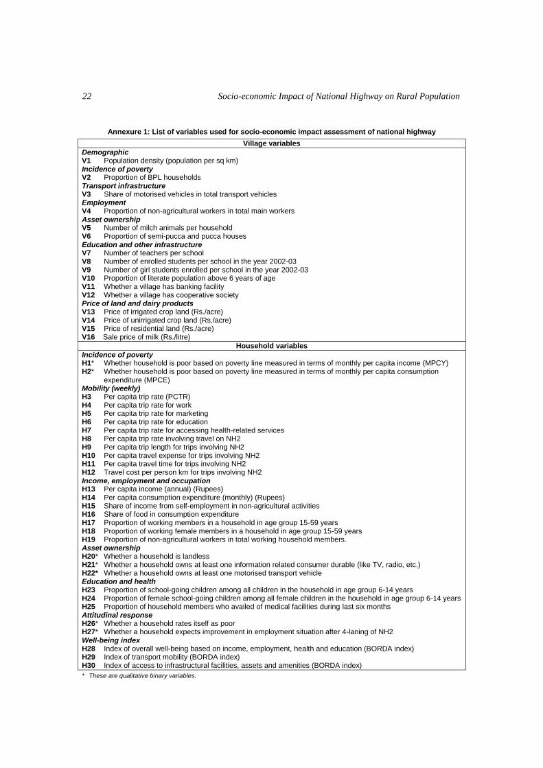
Socio-economic Impact of National Highway on Rural Population 22
Annexure 1: List of variables used for socio-economic impact assessment of national highway
Village variables
Demographic V1 Population density (population per sq km) Incidence of poverty V2 Proportion of BPL households Transport infrastructure V3 Share of motorised vehicles in total transport vehicles Employment V4 Proportion of non-agricultural workers in total main workers Asset ownership V5 Number of milch animals per household V6 Proportion of semi-pucca and pucca houses Education and other infrastructure V7 Number of teachers per school V8 Number of enrolled students per school in the year 2002-03 V9 Number of girl students enrolled per school in the year 2002-03 V10 Proportion of literate population above 6 years of age V11 Whether a village has banking facility V12 Whether a village has cooperative society Price of land and dairy products V13 Price of irrigated crop land (Rs./acre) V14 Price of unirrigated crop land (Rs./acre) V15 Price of residential land (Rs./acre) V16 Sale price of milk (Rs./litre)
Household variables
Incidence of poverty H1* Whether household is poor based on poverty line measured in terms of monthly per capita income (MPCY) H2* Whether household is poor based on poverty line measured in terms of monthly per capita consumption
expenditure (MPCE) Mobility (weekly) H3 Per capita trip rate (PCTR) H4 Per capita trip rate for work H5 Per capita trip rate for marketing H6 Per capita trip rate for education H7 Per capita trip rate for accessing health-related services H8 Per capita trip rate involving travel on NH2 H9 Per capita trip length for trips involving NH2 H10 Per capita travel expense for trips involving NH2 H11 Per capita travel time for trips involving NH2 H12 Travel cost per person km for trips involving NH2 Income, employment and occupation H13 Per capita income (annual) (Rupees) H14 Per capita consumption expenditure (monthly) (Rupees) H15 Share of income from self-employment in non-agricultural activities H16 Share of food in consumption expenditure H17 Proportion of working members in a household in age group 15-59 years H18 Proportion of working female members in a household in age group 15-59 years H19 Proportion of non-agricultural workers in total working household members. Asset ownership H20* Whether a household is landless H21* Whether a household owns at least one information related consumer durable (like TV, radio, etc.) H22* Whether a household owns at least one motorised transport vehicle Education and health H23 Proportion of school-going children among all children in the household in age group 6-14 years H24 Proportion of female school-going children among all female children in the household in age group 6-14 years H25 Proportion of household members who availed of medical facilities during last six months Attitudinal response H26* Whether a household rates itself as poor H27* Whether a household expects improvement in employment situation after 4-laning of NH2 Well-being index H28 Index of overall well-being based on income, employment, health and education (BORDA index) H29 Index of transport mobility (BORDA index) H30 Index of access to infrastructural facilities, assets and amenities (BORDA index)
* These are qualitative binary variables.

Methodology of Impact Evaluation 23
Annexure 2
Logit Regression Analysis
An important ingredient of PSMT is the logit analysis used to estimate
propensity scores. It is a convenient econometric tool for the analysis of a bi-variate
(or multivariate) data set comprising a binary qualitative dependent variable (see
Maddala (1986))36
. This technique is briefly explained below:
Consider a population in which some units possess a particular feature (e.g., in
a population of households some are poor). If a unit is picked up from the population
at random, the probability that the selected unit will have the feature depends on a
deterministic factor (that is a function of a set of explanatory variables) plus a random
error. Now, suppose a random sample of n households is drawn from the population.
Let yi = 1, if the ith sample household is observed to have the feature and 0 otherwise,
and ),...,,( 21 kiiii xxxx is the observed values of the relevant explanatory variables for
the ith sample unit (i = 1, 2,…, n, there being n sample households).
To explain the observed variation of the sample iy values, the following latent
variable regression model is specified: ,,...,2,1,* nixy iii where *y is an
unobservable variable, },...,,{ 21 k is the vector of coefficients associated with
k explanatory variables and si ' are random disturbances. Given this relationship, for
a sample unit with a given set of values of explanatory variables
otherwise 0 isit and 0 if 1 * ii yy37
. Now, it is assumed that the random
disturbances i ’s are identically distributed following a logistic distribution. That
means, Prob ( 1iy )=)exp(1
1
ii
xp
, or equivalently i
i
i xp
p
1
38 .
Given the sample observations ( nixy ii ,...,2,1,, ), the logit model is
estimated by maximum likelihood method. Once the estimation has been done, the
36. Maddala, G. S., Limited-dependent and qualitative variables in econometrics, Chapter 2, Cambridge
University Press, Cambridge, 1986.
37. In other words, ii xy i if 1 .
38. Note that the latter expression shows that odds ratio is a linear function of the explanatory variables under the
logit model.
Socio-economic Impact of National Highway on Rural Population 24
odds ratio can be calculated for the individual sample39
to derive the probability
measure of a household to fall in the influence zone.
39. However, before using the estimated probabilities and/or the corresponding odds ratios one should ensure that
the model has fitted satisfactorily to the given data set in the sense that the classification of the sample units
based on the estimated ex ante probabilities matches fairly well with the corresponding observed
classification. Along with the estimated parameter values, their standard errors and the maximised log-
likelihood value, values of other relevant sample statistics are provided by standard econometric software.
While these may be adequate for performing standard tests of hypotheses that are often required, there does
not exist any straightforward technique for visualising the performance in terms of the goodness of fit of the
estimated logit model (i.e. whether the classification of sample units based on estimated probabilities would
closely match the observed classification). It may, however, be possible to devise some ad hoc empirical
devices for such goodness of fit examination.
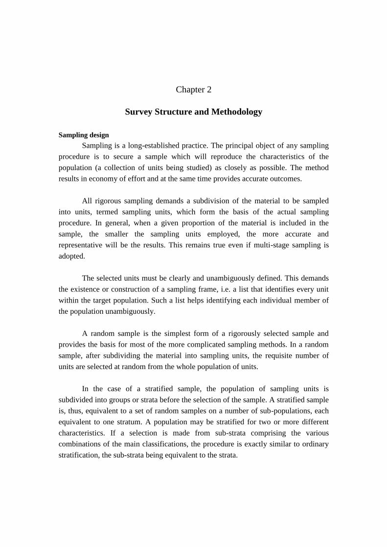
Chapter 2
Survey Structure and Methodology
Sampling design
Sampling is a long-established practice. The principal object of any sampling
procedure is to secure a sample which will reproduce the characteristics of the
population (a collection of units being studied) as closely as possible. The method
results in economy of effort and at the same time provides accurate outcomes.
All rigorous sampling demands a subdivision of the material to be sampled
into units, termed sampling units, which form the basis of the actual sampling
procedure. In general, when a given proportion of the material is included in the
sample, the smaller the sampling units employed, the more accurate and
representative will be the results. This remains true even if multi-stage sampling is
adopted.
The selected units must be clearly and unambiguously defined. This demands
the existence or construction of a sampling frame, i.e. a list that identifies every unit
within the target population. Such a list helps identifying each individual member of
the population unambiguously.
A random sample is the simplest form of a rigorously selected sample and
provides the basis for most of the more complicated sampling methods. In a random
sample, after subdividing the material into sampling units, the requisite number of
units are selected at random from the whole population of units.
In the case of a stratified sample, the population of sampling units is
subdivided into groups or strata before the selection of the sample. A stratified sample
is, thus, equivalent to a set of random samples on a number of sub-populations, each
equivalent to one stratum. A population may be stratified for two or more different
characteristics. If a selection is made from sub-strata comprising the various
combinations of the main classifications, the procedure is exactly similar to ordinary
stratification, the sub-strata being equivalent to the strata.

Socio-economic Impact of National Highway on Rural Population
26
In multi-stage sampling, the material is made up of a number of first-stage
sampling units, each of which, in turn, is made up of a number of second-stage units,
etc. The sampling procedure is carried out in stages. In the first stage, the first-stage
units are selected by a suitable method such as random or stratified sampling. In the
second stage, a sample of second-stage units is selected from among the selected first-
stage units by a method which may be the same or different from the method
employed for selecting the first-stage units. Further stages may be added as required.
Multi-stage sampling, thus, introduces an element of flexibility into sampling design
and enables utilising of the existing natural divisions and subdivisions of the material.
In the choice of the sampling frame, the following considerations were also
taken note of:
(i) Almost all surveys in general and surveys of households in particular
are multipurpose enquiries. They are designed to estimate numerous
characteristics on a variety of topics and sub-topics.
(ii) Just as a survey is seldom designed to measure a single variable,
similarly, it is seldom designed to measure variables at a single level of
aggregation.
Scope of the enquiry
The scope of the enquiry was confined to the rural population.
General design
The sample design was based on an appropriate stratification of village and
household units in order to make sampling units homogeneous within each stratum.
The general scheme of the sampling plan was a stratified two-stage design with
census villages as the first stage units (FSUs) and households within the sample
villages as the second stage units (SSUs). It may be mentioned that a stratified design
takes care of the variability factors and the two-stage design addresses the problem of
non-availability of a usable frame of the ultimate sampling units.
Delimiting influence zone
As mentioned in Chapter 1, a contiguous band of 5 km on both sides of NH2
has been taken to be the influence zone1.
1. The influence zone limits impact assessment analysis as the adaptation of the impact assessment method and
the definition of a zone of influence are interdependent, because both are a function of the characteristics of
the road and the surrounding area.

Survey Structure and Methodology
27
Identification of representative stretches
The national highway between Agra and Dhanbad extends over a distance of
995 km. Subjecting this entire length to a detailed survey would have involved huge
resources. It was, therefore, postulated that the purpose would be adequately served if
the scope of the enquiry were confined to representative stretches covering around 25
percent of the distance, i.e. 200-250 km of the road length. Thus, the foremost task
was to identify homogeneous and representative stretches spanning the three states of
Uttar Pradesh, Bihar and Jharkhand. The following criteria were adopted for the
purposes of selecting the stretches:
(i) should essentially cover rural areas;
(ii) should have homogeneous agro-climatic characteristics;
(iii) should be representative of the incidence of poverty in the district
concerned;
(iv) should form part of a single planning unit.
Rural coverage
The national highway passes through both rural and urban areas. Since the
focus of the present study is the rural population, the stretches have, essentially, to lie
in the rural areas. Therefore, while selecting each stretch, care was taken to identify a
contiguous segment of rural areas not having any urban habitation.
Agro-climatic regions
The agro-climatic characteristics of a region refer to soil quality, climate,
rainfall, and water resources. Based on these characteristics, the Planning
Commission has divided the country into the following 15 agro-climatic regions,
which have been further divided into sub-regions. The purpose of this division is to
promote farming systems of optimum crop production suited to the related agro-
climatic features.
(i) Western Himalayan (ii) Eastern Himalayan (iii) Lower Gangetic Plains
(iv) Middle Gangetic Plains (v) Upper Gangetic Plains (vi) Trans- Gangetic Plains
(vii) Eastern Plateau and Hills (viii) Central Plateau and Hills (ix) Western Plateau and Hills
(x) Southern Plateau and Hills (xi) East Coast Plains and Hills (xii) West Coast Plains and Ghats
(xiii) Gujarat Plains and Hills (xiv) Western Dry (xv) Islands
NH2 falls in three agro-climatic regions and five sub-regions. Care was taken
that the chosen stretches were representative of these regions and sub-regions, as
shown in Table 1.
Socio-economic Impact of National Highway on Rural Population
28
Table 1: State and district-wise agro-climatic sub-region distribution
State District Agro-climatic region Sub-region Chosen
stretches for survey purpose
Uttar Pradesh Agra Upper Gangetic Plain South Western Plains
Uttar Pradesh Firozabad Upper Gangetic Plain South Western Plains
Uttar Pradesh Etawah Upper Gangetic Plain South Western Plains
Uttar Pradesh Auraiya Upper Gangetic Plain South Western Plains
Uttar Pradesh Kanpur Dehat Upper Gangetic Plain South Western Plains
Uttar Pradesh Kanpur Nagar Upper Gangetic Plain South Western Plains
Uttar Pradesh Fatehpur Upper Gangetic Plain Central Plains
Uttar Pradesh Kaushambi Upper Gangetic Plain Central Plains
Uttar Pradesh Allahabad Upper Gangetic Plain Central Plains
Uttar Pradesh Sant Ravidas Nagar Middle Gangetic Plain Eastern Plains
Uttar Pradesh Varanasi Middle Gangetic Plain Eastern Plains
Uttar Pradesh Chandauli Middle Gangetic Plain Eastern Plains
Bihar Bhabua Middle Gangetic Plain South Bihar Plains
Bihar Rohtas Middle Gangetic Plain South Bihar Plains
Bihar Aurangabad Middle Gangetic Plain South Bihar Plains
Bihar Gaya Middle Gangetic Plain South Bihar Plains
Jharkhand Chatra Eastern Plateau & Hill Regions Chotta Nagpur Hills
Jharkhand Hazaribagh Eastern Plateau & Hill Regions Chotta Nagpur Hills
Jharkhand Giridih Eastern Plateau & Hill Regions Chotta Nagpur Hills
Jharkhand Koderma Eastern Plateau & Hill Regions Chotta Nagpur Hills
Jharkhand Bokaro Eastern Plateau & Hill Regions Chotta Nagpur Hills
Jharkhand Dhanbad Eastern Plateau & Hill Regions Chotta Nagpur Hills
Source: NSSO, Government of India, 1993-94 and Alagh, Y. K, ‘Land and Man: Essays in Sustainable Development’, 1996.
Incidence of poverty
Estimating poverty and identifying the poor, though closely related, are not
one and the same. The first is a task assigned to the Planning Commission and is done
through sample surveys on consumer expenditure conducted by the National Sample
Survey Organisation (NSSO). The identification of the poor is done through door-to-
door surveys with total coverage. The state governments under the overall direction of
the Union Ministry of Rural Development carry out these surveys. The census results
give an estimate of the percentage and number of poor households at the village,
block, district and state levels, while the NSSO surveys estimate poverty at the state
level.
While estimating poverty helps in assessing its magnitude, the identification of
specific households living ‘below the poverty line’ is necessary for targeting them
under various poverty alleviation programmes. We have, therefore, used the latter
data while selecting the stretches. Care was taken that, as far as possible, only areas
with reported higher incidence of poverty were covered. For instance, in Uttar
Pradesh, the highest incidence of poverty was reported in Auraiya district where 47.96
percent of the households were enumerated as BPL. A stretch falling in this district
was, therefore, included. Similarly, in Bihar, a stretch falling in Gaya district, with a

Survey Structure and Methodology
29
reported BPL household percentage of 69.83 and in Jharkhand, a stretch falling in the
district of Hazaribagh with a reported BPL household percentage of 66.18, was
included.
Planning unit
A single planning unit was taken as one of the criteria for choosing the
stretches because it would help to understand a self-sustaining region while evaluating
a specific programme. Such a unit can be defined as an area having economic and
administrative homogeneity. It is large enough to enable substantial changes in
distribution and employment to take place within its boundaries, yet is small enough
for its planning problems to be seen as a whole. In India, for the purpose of national
planning, a district is taken as a planning unit. Care was, therefore, taken that a stretch
fell in a single district and there was no overlap either across the districts or the states.
Formation of basic strata
Seven road stretches covering a total of 264 km of road length have been
demarcated out of 995 km of the highway falling in the states of Uttar Pradesh, Bihar
and Jharkhand. Each stretch is homogeneous with respect to agro-climatic
characteristics and the incidence of poverty and is synchronised with planning and
administrative geographic area. The details of the stretches are outlined in Table 2
below.
Table 2: Details of stretches
Stretch District State Length
(km) District level %
of poverty
Asfafabad-Mithepur Firozabad Uttar Pradesh 47 15.48
Lalpur-Purwa Rahat Auraiya Uttar Pradesh 27 47.96
Galtha-Sangaon Fatehpur Uttar Pradesh 37 31.73
Dahia-Naubatpur Chandauli Uttar Pradesh 36 34.70
Mahwaria-Khosmabad Bhabhua Bihar 47 43.04
Bairbigha-Barachatti Gaya Bihar 39 69.83
Barhi-Laimbua Hazaribagh Jharkhand 31 66.18
General characteristics of the basic strata
The four stretches in the state of Uttar Pradesh fall in the districts of
Firozabad, Auraiya, Fatehpur, and Chandauli. The two stretches in Bihar lie in the
districts of Bhabhua and Gaya. The stretch in Jharkhand falls in the district of
Hazaribagh. In these selected stretches, 1,697 villages lying in the horizontal distance
band of 0-7 km on both sides of NH2 were identified. This distance band covers both

Socio-economic Impact of National Highway on Rural Population
30
the influence and the control zones. Table 3 shows the stretch-wise distribution of
villages, population and residential households based on the 1991 census.
Table 3: Formation of basic strata
Stretch District No. of
villages Population
Residential households
I Firozabad 243 306603 46420
II Auraiya 162 184546 27735
III Fatehpur 170 224491 37874
IV Chandauli 332 384630 52921
V Bhabhua 254 230709 29237
VI Gaya 417 323096 45084
VII Hazaribagh 119 114028 14130
Total 1697 1768103 253401
The strata falling in the states of Uttar Pradesh and Bihar are endowed with the
water resources of the rivers Yamuna and Ganga, good annual rainfall in the range of
550-900 mm, and fertile alluvial soil of the Indo-Gangetic Plain. According to the
village directory of the Census of India 1991, the people living in these stretches have
a fairly enough drinking water, access to educational facilities, and power supply.
They are, however, poor in health facilities, and transport and communication
connectivity.
Basic Strata I to IV, which fall in Uttar Pradesh, are homogeneous with
respect to physiographic characteristics, irrigation, power supply, education, health
and connectivity. Annual rainfall in this region is in the range of 550-700 mm and
relative humidity during the driest part of the year is below 20 percent. Principal crops
are wheat, rice, sugarcane, pulses and potatoes. The availability of canal and tube-well
water and power supply is reasonably good.
Basic Strata V to VII falling in Bihar and Jharkhand have high rainfall (more
than 700 mm in a year) and high relative humidity. The cropping pattern, therefore,
changes in favour of paddy. The area is characterised by low irrigation and power
supply, lower educational facilities, and still lower health facilities. In the case of
Stretch VII in Jharkhand, which lies in the sub-region of Chotta Nagpur hills, the soil
type changes so also the physiographic characteristics.
Further insights into the socio-economic profile of the basic strata and the
infrastructural facilities available therein may be had from the details presented in
Annex 1.
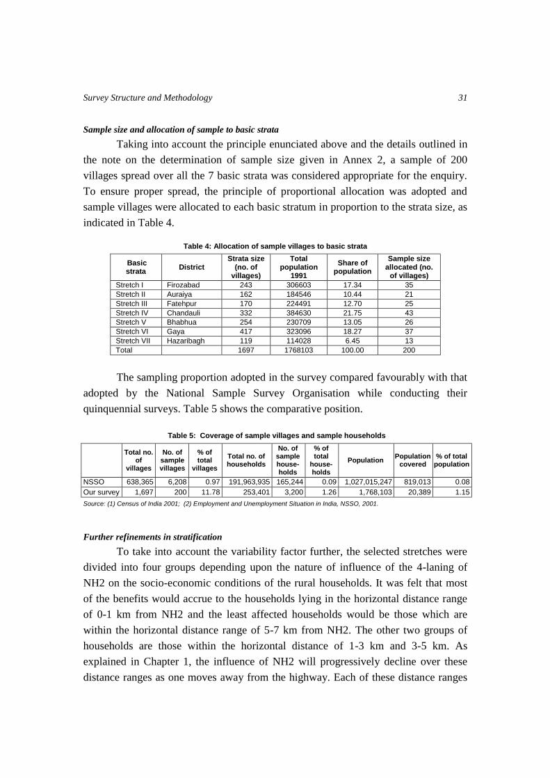
Survey Structure and Methodology
31
Sample size and allocation of sample to basic strata
Taking into account the principle enunciated above and the details outlined in
the note on the determination of sample size given in Annex 2, a sample of 200
villages spread over all the 7 basic strata was considered appropriate for the enquiry.
To ensure proper spread, the principle of proportional allocation was adopted and
sample villages were allocated to each basic stratum in proportion to the strata size, as
indicated in Table 4.
Table 4: Allocation of sample villages to basic strata
Basic strata
District Strata size
(no. of villages)
Total population
1991
Share of population
Sample size allocated (no.
of villages)
Stretch I Firozabad 243 306603 17.34 35
Stretch II Auraiya 162 184546 10.44 21
Stretch III Fatehpur 170 224491 12.70 25
Stretch IV Chandauli 332 384630 21.75 43
Stretch V Bhabhua 254 230709 13.05 26
Stretch VI Gaya 417 323096 18.27 37
Stretch VII Hazaribagh 119 114028 6.45 13
Total 1697 1768103 100.00 200
The sampling proportion adopted in the survey compared favourably with that
adopted by the National Sample Survey Organisation while conducting their
quinquennial surveys. Table 5 shows the comparative position.
Table 5: Coverage of sample villages and sample households
Total no.
of villages
No. of sample villages
% of total
villages
Total no. of households
No. of sample house-holds
% of total
house-holds
Population Population
covered % of total
population
NSSO 638,365 6,208 0.97 191,963,935 165,244 0.09 1,027,015,247 819,013 0.08
Our survey 1,697 200 11.78 253,401 3,200 1.26 1,768,103 20,389 1.15
Source: (1) Census of India 2001; (2) Employment and Unemployment Situation in India, NSSO, 2001.
Further refinements in stratification
To take into account the variability factor further, the selected stretches were
divided into four groups depending upon the nature of influence of the 4-laning of
NH2 on the socio-economic conditions of the rural households. It was felt that most
of the benefits would accrue to the households lying in the horizontal distance range
of 0-1 km from NH2 and the least affected households would be those which are
within the horizontal distance range of 5-7 km from NH2. The other two groups of
households are those within the horizontal distance of 1-3 km and 3-5 km. As
explained in Chapter 1, the influence of NH2 will progressively decline over these
distance ranges as one moves away from the highway. Each of these distance ranges
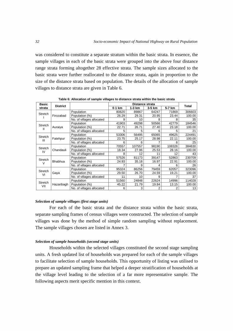
Socio-economic Impact of National Highway on Rural Population
32
was considered to constitute a separate stratum within the basic strata. In essence, the
sample villages in each of the basic strata were grouped into the above four distance
range strata forming altogether 28 effective strata. The sample sizes allocated to the
basic strata were further reallocated to the distance strata, again in proportion to the
size of the distance strata based on population. The details of the allocation of sample
villages to distance strata are given in Table 6.
Table 6: Allocation of sample villages to distance strata within the basic strata
Basic strata
District Distance strata
Total 0-1 km 1-3 km 3-5 km 5-7 km
Stretch I
Firozabad
Population 80620 89867 64247 71869 306603
Population (%) 26.29 29.31 20.95 23.44 100.00
No. of villages allocated 9 10 8 8 35
Stretch II
Auraiya
Population 41903 49298 50566 42779 184546
Population (%) 22.71 26.71 27.40 23.18 100.00
No. of villages allocated 5 5 6 5 21
Stretch III
Fatehpur
Population 53306 56495 65065 49625 224491
Population (%) 23.75 25.17 28.98 22.11 100.00
No. of villages allocated 6 6 7 6 25
Stretch IV
Chandauli
Population 70557 107557 98190 108326 384630
Population (%) 18.34 27.96 25.53 28.16 100.00
No. of villages allocated 8 12 11 12 43
Stretch V
Bhabhua
Population 57526 81173 39147 52863 230709
Population (%) 24.93 35.18 16.97 22.91 100.00
No. of villages allocated 7 9 4 6 26
Stretch VI
Gaya
Population 95324 86256 79459 62057 323096
Population (%) 29.50 26.70 24.59 19.21 100.00
No. of villages allocated 11 10 9 7 37
Stretch VII
Hazaribagh
Population 51560 24848 22624 14996 114028
Population (%) 45.22 21.79 19.84 13.15 100.00
No. of villages allocated 6 3 2 2 13
Selection of sample villages (first stage units)
For each of the basic strata and the distance strata within the basic strata,
separate sampling frames of census villages were constructed. The selection of sample
villages was done by the method of simple random sampling without replacement.
The sample villages chosen are listed in Annex 3.
Selection of sample households (second stage units)
Households within the selected villages constituted the second stage sampling
units. A fresh updated list of households was prepared for each of the sample villages
to facilitate selection of sample households. This opportunity of listing was utilised to
prepare an updated sampling frame that helped a deeper stratification of households at
the village level leading to the selection of a far more representative sample. The
following aspects merit specific mention in this context.
Survey Structure and Methodology
33
Listing: To control the workload at the listing stage, it was postulated that a
maximum of 200 households in a village would be enough to select 16 sample
households (ultimate stage units). This number was considered to be fairly adequate
for the purpose of using it as sampling frame. If the number of households in a village
exceeded 200, the following procedure was adopted for selecting the 200 households
for listing. A rough estimate of the number of households in each hamlet (tola) of a
village was obtained from the head (Pradhan/Sarpanch) of the village. The number of
households to be listed in a hamlet was then obtained by multiplying the share of
hamlet households to the total number of village households with 200. For example, if
a village had 1,000 households residing in five hamlets and in one hamlet, the number
of households was 400, the proportion of households in this hamlet to the total
number of households would be 400/1000 = 0.40. Thus, the number of households to
be listed in that hamlet would work out to 0.40 200 = 80. Every fifth household
would thus be listed in that particular hamlet.
Sub-stratification: At the time of listing, all the households in a village were
classified in the categories of ‘affluent households’ and ‘the rest’. A household was
treated as affluent if it owned items like car/jeep, colour TV, telephone, consumer
durables like VCR, or refrigerator; or owned a large well-maintained pucca house, or
owned land in excess of 20 acres of cultivable land or 10 acres of irrigated land; or
where at least one member of the household had a well-paid salaried job or was
engaged in a profession with handsome income, like doctor, advocate, etc.; or was the
owner of a large business establishment.
Information relating to the major sources of income of each household was
also collected. The households were categorised as ‘self-employed in non-agriculture’
or ‘rural labour’ or ‘others’ on the basis of this information.
All the households listed in a sample village were segregated into two second
stage strata, viz. ‘affluent households’ (forming second stage stratum 1) and ‘the rest’
(forming second stage stratum 2). The latter stratum was further stratified into three
categories: self-employed in non-agriculture, rural labour, and others. The size of
sample households in stratum 2 was in proportion to the number of households in
each of these categories.
Socio-economic Impact of National Highway on Rural Population
34
Procedure for the selection of households
A total of 16 households were selected from each sample village as follows:
(i) Two sample households from ‘affluent households’ (sub-strata 1)
circular systematically with a random start.
(ii) Fourteen sample households from sub-strata 2. These were selected
from the rest of the households circular systematically with a random
start.
Survey schedules
In order to generate data on village and household characteristics as well as
different socio-economic causal factors and outcomes of the developmental
intervention of four-laning of NH2, extensive schedules were prepared for the primary
baseline survey with emphasis on the following, and the pre-testing of the schedules
was done before their finalisation.
(i) Enable collection of accurate information to meet the needs in a timely
manner;
(ii) Facilitate the work of data collection, processing and tabulation;
(iii) Ensure economy in data collection; and
(iv) Permit comprehensive and meaningful analysis and purposeful
utilisation of data collected.
Since the present study is the first of its kind in the country, we utilised the
inputs of the researchers in the World Bank in preparing detailed schedules. We also
had the benefit of the advice of the National Sample Survey Organisation (NSSO),
which has wide experience in undertaking socio-economic household surveys in the
country. In addition, we referred to the questionnaires used by the Census of India to
elicit information on economic variables and also benefited from the related surveys
carried out by different research institutions.
Both the village and household schedules are fairly comprehensive and some
of the information collected may not be utilised for the socio-economic impact
analysis. It was, however, felt that the same would be useful as a qualitative input for
the participatory rural appraisal for which a separate exercise was carried out. The
data would also be useful for further research in different aspects of socio-economic
conditions at the regional level. Care was, however, taken that the length of the
schedules in no way fatigued the respondent and the investigator during the course of
the interview.

Survey Structure and Methodology
35
The schedules provide detailed information relating to the coordinates of the
sample villages and sample households. This would help in identifying the same set of
villages and households which would be surveyed in the follow-up exercise after a
lapse of 4-5 years. The schedules also show the dates when the survey was carried out
so that the follow-up survey is carried out in the same period to the extent possible so
as to eliminate seasonality factor bias.
A broad format of the socio-economic variables detailed in the village and
household survey schedules is given in Box 1. These variables can be clubbed into
three broad categories relating to transport; income and expenditure; and social
aspects.
Box 1: List of variables
(i) Transport variables
Connectivity to national highway Type of road connectivity from village to NH Distance of the village from NH
Accessibility Nearest distance of the village to different facilities (e.g., market, urban centre, educational institution, medical facility, etc.)
Traffic density Availability of public transport Frequency of public transport (bus, jeep, taxi, tempo, etc)
Fares and costs Passenger fares Transport cost of agricultural inputs (seeds, fertilisers, pesticides) Transport cost of agricultural products Transport cost of non-agricultural products
Transport patterns Number of trips taken outside village, by purpose Time required to reach selected destinations (nearest city, market, school, health centre, workplace.) Main mode of transport to selected destinations
Vehicle ownership Ownership of vehicles (motorised and non-motorised)
(ii) Income and expenditure variables
Impact on agricultural activities Land use pattern Ownership of land Land devoted to different crops Output of key crops per unit of cultivated land Amount of harvest sold in markets Use of improved seeds, fertilizers, herbicides, pesticides Use of farm equipment (tractors, machines) Farm-gate prices of key crops Unit price of farm inputs Number of people (household members, other) working on farm Agricultural wage rate Livestock ownership Evacuation of agricultural surplus
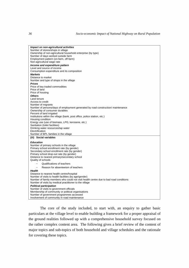
Socio-economic Impact of National Highway on Rural Population
36
Impact on non-agricultural activities Number of stores/shops in village Ownership of non-agricultural household enterprise (by type) Number of days worked outside farm Employment pattern (on-farm, off-farm) Non-agricultural wage rate
Income and expenditure pattern Level and source of income Consumption expenditure and its composition
Markets Distance to market Number and type of shops in the village
Prices Price of key traded commodities Price of land Price of housing
Others Land tenure Access to credit Number of migrants Number of persons/days of employment generated by road construction/ maintenance Ownership of consumer durables Percent of land irrigated Institutions within the village (bank, post office, police station, etc.) Housing condition Energy use (use of biomass, LPG, kerosene, etc.) Sanitation (toilet facilities) Drinking water resources/tap water Electrification Number of BPL families in the village
(iii) Social variables
Education Number of primary schools in the village Primary school enrollment rate (by gender) Secondary school enrollment rate (by gender) Primary school drop-out rate (by gender) Distance to nearest primary/secondary school Quality of schools
Qualifications of teachers
Reason for absenteeism of teachers
Health Distance to nearest health centre/hospital Number of visits to health facilities (by age/gender) Number of family members who could not visit health centre due to bad road conditions Number of visits by medical practitioner to the village
Political participation Number of visits to government officials Membership of community or political organisations Number of government programmes accessed Involvement of community in road maintenance
The core of the study included, to start with, an enquiry to gather basic
particulars at the village level to enable building a framework for a proper appraisal of
the ground realities followed up with a comprehensive household survey focused on
the rather complex content area. The following gives a brief review of the content of
major topics and sub-topics of both household and village schedules and the rationale
for covering these topics.
Survey Structure and Methodology
37
Household schedule
Household characteristics
The schedule provides a general overview of household characteristics such as
household size, social and religious status, and inward migration. This data are
relevant for the purpose of analysis and are included as basic particulars.
Roster of household members
The household roster records the composition of the household and collects
basic socio-economic information about its members (age, gender, marital status,
educational attainments, occupation, etc.). Information on place of work, travel time
and modes of transport is also included under this section.
Household economic activities
In rural areas, members of many households are engaged in self-employment.
Most of such activities are seasonal. Taking this feature into account, efforts have
been made to design the survey instrument in such a way as to reflect these
characteristics adequately. For this purpose, the standardised concept of activity status
has been adopted as per the National Industrial Classification Code 1998 of the
Central Statistical Organisation, Government of India.
Housing and amenities
Data on housing and other amenities are necessary as supplementary
information. The schedule obtains information on the type of housing and available
amenities (drinking water, electricity, energy use, sanitation).
Assets holding
Assets holding constitutes a major factor while assessing the standard of living
of the people residing in the rural areas. Hence, information relating to assets holding
(consumer durables, production equipment, vehicle ownership, etc.) has been
collected in sufficient detail indicating, inter alia, the purchases during the last 12
months and the expenditure incurred on the same.

Socio-economic Impact of National Highway on Rural Population
38
Landholding and agricultural production
The schedule includes information on landholding and agricultural production.
This covers the total operational landholding of the household, and area under
different crops and the total produce, including agricultural byproducts. To understand
the role of transport in the evacuation of agricultural surplus, information was sought
on modes of transport used and the cost involved for the same.
Livestock
Livestock is an important source of livelihood in the rural areas. The schedule
seeks information on the livestock ownership, yield of animal products, and
expenditure incurred on livestock maintenance. Special attention has been given to the
role of transportation in the evacuation of animal products by collecting information
on modes of transport used and the cost involved for the same.
Non-farm sector
An important aspect of road development is to measure its impact on the non-
farm sector. The schedule addresses this aspect by incorporating information on non-
agricultural enterprises, employment and productivity in such enterprises. The
schedule also seeks detailed information on informal units. To enable accounting
without omission or duplication, efforts were made to gather separate details for
entrepreneurial activities in handicraft or cottage industries and other income-
generating activities in trade, transport, communication, personal services, etc. To
have a better idea about the role of transportation in the growth of the non-farm
sector, the process of evacuation of non-agricultural products and transportation costs
involved are also incorporated in the schedule.
Household income
Conceptually, household income is the sum of money income and income in
kind and consists of receipts which, as a rule, are of a recurring nature and accrue to
household members regularly at frequent intervals. It includes individual income of
all household members and the combined income of the household, either in cash or
kind. The schedule comprises information on income from agriculture (including
livestock), self-employment in non-agriculture, salary or wage-paid employment, and
income from other sources. Taking into account the difficulties and complexities
involved in the measurement of income, especially in the context of the likely
preponderance of self-employment activities, special efforts have been made to
Survey Structure and Methodology
39
provide for all possible cases through a detailed structured approach. The household
income relates to a period of one year preceding the date of survey.
Consumption expenditure
Monthly consumption expenditure is an important aspect when measuring the
standard of living of the rural population. The schedule, therefore, seeks detailed
information on both food and non-food items. In the case of food items, the recall
period has been limited to 30 days, while in the case of non-food items, the recall
period varies between 30 days and 365 days.
Education
Information on education has been collected in a detailed manner so as to
assess the impact of the project on the educational attainment of the household
members. In addition to the current educational status, the survey was also designed
to understand the problems and prospects of children in the age-group 6-15 years in
pursuing education in institutions located within and outside the village. Of special
interest was the detailed recording of distance from educational institutions, time and
modes of transport.
Health
Health is a principal component of social consumption. It is important to
collect information about the extent to which medical and health services and
facilities available in and around the village are availed of by the household members.
Marginally extending the scope of health-related information, the issue of the mobility
of members in availing of health facilities in terms of distance travelled, mode of
transport and time taken in travel were also enquired into.
Participation in community affairs
Road construction and improvement may not only facilitate access to
education and health facilities but may also enhance social interaction and political
participation. The purpose of the schedule is also to capture the household’s
involvement in these aspects of community life. Social attitudes, gender
discrimination, attendance at social and political events in and outside the village are
some of the issues that are included in the schedule.

Socio-economic Impact of National Highway on Rural Population
40
Diary of travel activity
To see the direct effects of road development in terms of the mobility of
household members, special provision has been made in the schedule to obtain travel-
related information through the approach of origin-destination trips. Trip has been
defined as one-way movement of a person by any mode of transport having two trip
ends – an origin or start of a trip and a destination or end of a trip – for a specific
purpose. For the current study, only information on trips outside the village was
collected; information on trips within the village was not recorded. The travel diary
also seeks information on trip purpose, trip length, mode of transport used, and use of
national highway in the course of a trip, travel cost and time. In order to control errors
and bias creeping into the data, the reference period for capturing the details was kept
at the optimal level of seven days prior to the date of enquiry.
Information on household members’ preferred mode of travel, their attitudinal
response to development activities in the village, their perception and opinion on the
highway development project, etc. would be very significant to supplement the
database. Adequate provision to gather data on these aspects has been made in the
household schedule.
Village schedule
General characteristics
The schedule provides a general overview of the demographic characteristics
of the villages (population size, social/religious composition), and their major social
and economic infrastructure (including health, education, and transport
infrastructure).
Economic activities
The schedule adds the economic dimension to the general characteristics by
seeking information on various economic activities in the village. It covers the main
economic activities and resources of the village, and thus complements the household-
level economic data.
Education
The schedule obtains information on the inventory of the educational facilities
in the village (number and type of schools, classes and teachers) and indicators of
quality (educational qualifications of teachers, teachers’ credentials and attendance).
Survey Structure and Methodology
41
This information complements the enrollment and attendance data collected in the
household schedule. Information on enrollment rate and drop-out rate in the schools is
also elicited.
Health
Information on the inventory of the healthcare facilities in the village (number
and type of facilities and healthcare personnel) and indicators of quality (attendance
of doctors and nurses) is recorded in the schedule. This information was collected
from village Pradhan/Health Centre Personnel.
Transport infrastructure
The schedule seeks information on the state of the village transport
infrastructure. This refers to roads that connect or pass through the village, their
condition, distance from the national highway and state highway, distance to railway
station and waterways (where applicable), and the extent of available transport
services available. Information was also sought on difficulties experienced by the
villagers due to the poor quality of infrastructure and transport services.
Markets
The effect of road projects on the accessibility of markets is a critical factor in
bringing about changes in the pattern and level of income. The schedule obtains
information on the frequency and type of markets.
Prices
Changes in transport costs brought about by road projects are likely to affect
prices of tradable goods. The schedule records information on the prices of different
commodities in the market inside the village or in the nearby village/town.
Government programmes
There is every likelihood that the improvement in road infrastructure would
result in better coverage and would in turn enhance the quality of various
development programmes. Hence, information was sought on the number and type of
such programmes operating in the village and the extent to which they are availed of
by the residents (benefits accrued to the residents).

Socio-economic Impact of National Highway on Rural Population
42
Land use
Change in land use pattern is regarded as a major impact of road transport
development. As such, the schedule seeks village-wise information on land use
pattern. It also elicits information on the cropping pattern, price of land and tenancy
pattern.
Community activities
The schedule aims to provide an overview of the social and potential events
and activities in the village. The increased mobility and communication resulting from
better road connectivity may well have measurable social capital effects on villages,
which this schedule attempts to capture. This section complements the household
survey schedule, which covers the household participation in community affairs.
Method of enquiry
Considering the complexity of the subject matter, the necessity of obtaining
complete and consistent data and the advantages and limitations of various methods of
enquiry, it was considered appropriate to use the interview method or a combination
of interview and observation methods for the household enquiry.
Data input
The data was stored in the electronic form using the software MS ACCESS &
SPSS. Further tabulation for analysis was done in the MS EXCEL format after
appropriate mapping from MS ACCESS.
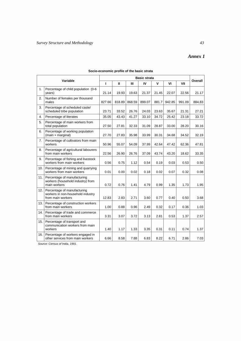
Survey Structure and Methodology
43
Annex 1
Socio-economic profile of the basic strata
Variable Basic strata
Overall I II III IV V VI VII
1. Percentage of child population (0-6 years) 21.14 19.93 19.63 21.37 21.45 22.07 22.56 21.17
2. Number of females per thousand males 827.66 818.89 868.59 899.07 881.7 942.85 991.09 884.83
3. Percentage of scheduled caste/ scheduled tribe population 23.71 33.52 26.76 24.03 23.63 35.67 21.31 27.21
4. Percentage of literates 35.05 43.43 41.27 33.10 34.72 25.42 23.18 33.72
5. Percentage of main workers from total population 27.50 27.81 32.33 31.09 28.87 33.00 28.20 30.16
6. Percentage of working population (main + marginal) 27.70 27.83 35.98 33.99 30.31 34.68 34.52 32.19
7. Percentage of cultivators from main workers 50.96 55.07 54.09 37.99 42.64 47.42 62.36 47.81
8. Percentage of agricultural labourers from main workers 22.56 26.90 26.76 37.09 43.74 43.20 18.62 33.35
9. Percentage of fishing and livestock workers from main workers 0.56 0.75 1.12 0.54 0.19 0.03 0.53 0.50
10. Percentage of mining and quarrying workers from main workers 0.01 0.00 0.02 0.18 0.02 0.07 0.32 0.08
11. Percentage of manufacturing workers (household industry) from main workers 0.72 0.76 1.41 4.79 0.99 1.35 1.73 1.95
12. Percentage of manufacturing workers in non-household industry from main workers 12.83 2.83 2.71 3.60 0.77 0.40 0.50 3.68
13. Percentage of construction workers from main workers 1.00 0.88 0.96 2.49 0.32 0.17 0.36 1.03
14. Percentage of trade and commerce from main workers 3.31 3.07 3.72 3.13 2.81 0.53 1.37 2.57
15. Percentage of transport and communication workers from main workers 1.40 1.17 1.33 3.35 0.31 0.11 0.74 1.37
16. Percentage of workers engaged in other services from main workers 6.66 8.58 7.88 6.83 8.22 6.71 2.86 7.03
Source: Census of India, 1991.
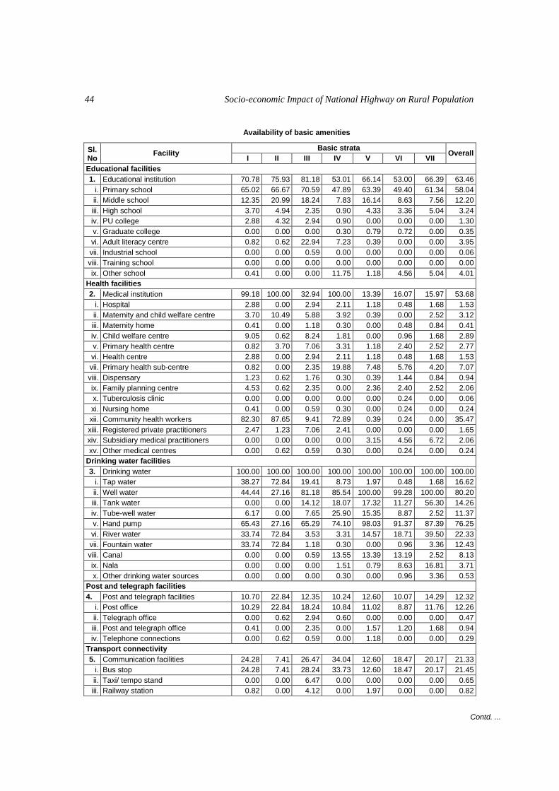
Socio-economic Impact of National Highway on Rural Population
44
Availability of basic amenities
Sl. No
Facility Basic strata
Overall I II III IV V VI VII
Educational facilities
1. Educational institution 70.78 75.93 81.18 53.01 66.14 53.00 66.39 63.46
i. Primary school 65.02 66.67 70.59 47.89 63.39 49.40 61.34 58.04
ii. Middle school 12.35 20.99 18.24 7.83 16.14 8.63 7.56 12.20
iii. High school 3.70 4.94 2.35 0.90 4.33 3.36 5.04 3.24
iv. PU college 2.88 4.32 2.94 0.90 0.00 0.00 0.00 1.30
v. Graduate college 0.00 0.00 0.00 0.30 0.79 0.72 0.00 0.35
vi. Adult literacy centre 0.82 0.62 22.94 7.23 0.39 0.00 0.00 3.95
vii. Industrial school 0.00 0.00 0.59 0.00 0.00 0.00 0.00 0.06
viii. Training school 0.00 0.00 0.00 0.00 0.00 0.00 0.00 0.00
ix. Other school 0.41 0.00 0.00 11.75 1.18 4.56 5.04 4.01
Health facilities
2. Medical institution 99.18 100.00 32.94 100.00 13.39 16.07 15.97 53.68
i. Hospital 2.88 0.00 2.94 2.11 1.18 0.48 1.68 1.53
ii. Maternity and child welfare centre 3.70 10.49 5.88 3.92 0.39 0.00 2.52 3.12
iii. Maternity home 0.41 0.00 1.18 0.30 0.00 0.48 0.84 0.41
iv. Child welfare centre 9.05 0.62 8.24 1.81 0.00 0.96 1.68 2.89
v. Primary health centre 0.82 3.70 7.06 3.31 1.18 2.40 2.52 2.77
vi. Health centre 2.88 0.00 2.94 2.11 1.18 0.48 1.68 1.53
vii. Primary health sub-centre 0.82 0.00 2.35 19.88 7.48 5.76 4.20 7.07
viii. Dispensary 1.23 0.62 1.76 0.30 0.39 1.44 0.84 0.94
ix. Family planning centre 4.53 0.62 2.35 0.00 2.36 2.40 2.52 2.06
x. Tuberculosis clinic 0.00 0.00 0.00 0.00 0.00 0.24 0.00 0.06
xi. Nursing home 0.41 0.00 0.59 0.30 0.00 0.24 0.00 0.24
xii. Community health workers 82.30 87.65 9.41 72.89 0.39 0.24 0.00 35.47
xiii. Registered private practitioners 2.47 1.23 7.06 2.41 0.00 0.00 0.00 1.65
xiv. Subsidiary medical practitioners 0.00 0.00 0.00 0.00 3.15 4.56 6.72 2.06
xv. Other medical centres 0.00 0.62 0.59 0.30 0.00 0.24 0.00 0.24
Drinking water facilities
3. Drinking water 100.00 100.00 100.00 100.00 100.00 100.00 100.00 100.00
i. Tap water 38.27 72.84 19.41 8.73 1.97 0.48 1.68 16.62
ii. Well water 44.44 27.16 81.18 85.54 100.00 99.28 100.00 80.20
iii. Tank water 0.00 0.00 14.12 18.07 17.32 11.27 56.30 14.26
iv. Tube-well water 6.17 0.00 7.65 25.90 15.35 8.87 2.52 11.37
v. Hand pump 65.43 27.16 65.29 74.10 98.03 91.37 87.39 76.25
vi. River water 33.74 72.84 3.53 3.31 14.57 18.71 39.50 22.33
vii. Fountain water 33.74 72.84 1.18 0.30 0.00 0.96 3.36 12.43
viii. Canal 0.00 0.00 0.59 13.55 13.39 13.19 2.52 8.13
ix. Nala 0.00 0.00 0.00 1.51 0.79 8.63 16.81 3.71
x. Other drinking water sources 0.00 0.00 0.00 0.30 0.00 0.96 3.36 0.53
Post and telegraph facilities
4. Post and telegraph facilities 10.70 22.84 12.35 10.24 12.60 10.07 14.29 12.32
i. Post office 10.29 22.84 18.24 10.84 11.02 8.87 11.76 12.26
ii. Telegraph office 0.00 0.62 2.94 0.60 0.00 0.00 0.00 0.47
iii. Post and telegraph office 0.41 0.00 2.35 0.00 1.57 1.20 1.68 0.94
iv. Telephone connections 0.00 0.62 0.59 0.00 1.18 0.00 0.00 0.29
Transport connectivity
5. Communication facilities 24.28 7.41 26.47 34.04 12.60 18.47 20.17 21.33
i. Bus stop 24.28 7.41 28.24 33.73 12.60 18.47 20.17 21.45
ii. Taxi/ tempo stand 0.00 0.00 6.47 0.00 0.00 0.00 0.00 0.65
iii. Railway station 0.82 0.00 4.12 0.00 1.97 0.00 0.00 0.82
Contd. ...

Survey Structure and Methodology
45
Sl. No
Facility Basic strata
Overall I II III IV V VI VII
Approach to village
iv. Pucca road 37.45 40.74 30.59 56.02 14.57 27.34 28.57 34.18
v. Katcha road 59.26 58.64 70.59 55.42 93.70 99.28 84.87 76.37
vi. Navigable river 0.00 0.00 8.82 1.20 0.00 2.16 2.52 1.83
vii. Navigable canal 0.00 0.00 0.59 0.30 1.18 0.00 0.00 0.29
viii. Footpath 3.70 0.62 34.12 12.05 0.00 0.00 7.56 6.89
Power supply
6. Power supply 83.95 51.23 85.29 90.06 83.07 46.76 33.61 69.36
i. Power supply for domestic purpose 30.04 35.80 44.12 62.35 22.44 1.20 14.29 28.99
ii. Power supply for agriculture 60.08 29.01 42.35 48.80 72.05 27.58 8.40 43.31
iii. Power supply for industrial/ commercial purpose 2.06 0.00 0.00 0.00 0.39 0.48 1.68 0.59
iv. Power for all purposes 25.93 3.09 28.24 17.77 10.63 17.51 11.76 17.03
Irrigation facilities
7. Irrigation facilities by
i. Well without electricity 0.78 0.01 0.52 0.00 5.69 11.53 30.64 4.00
ii. Well with electricity 1.66 2.45 0.32 0.29 28.60 2.98 1.88 5.10
iii. Tube-well with electricity 13.40 14.75 23.79 0.25 4.54 6.89 4.20 9.86
iv. Tube-well without electricity 54.87 9.71 30.62 0.89 14.03 1.20 0.15 19.25
v. Government canal 29.11 71.83 41.82 98.57 33.82 19.52 8.99 46.31
vi. Private canal 0.00 0.42 0.00 0.00 0.36 3.05 2.17 0.77
vii. River irrigation 0.05 0.00 0.00 0.00 1.61 2.91 17.31 1.17
viii. Tank irrigation 0.00 0.07 2.25 0.00 3.43 10.03 15.67 3.18
ix. Other source 0.13 0.75 0.69 0.00 7.92 41.89 18.99 10.35
Market facilities
8. Availability of market facilities 3.29 4.94 5.88 3.31 1.18 5.76 12.61 4.66
Source: Census of India, 1991.
Socio-economic Impact of National Highway on Rural Population
46
Annex 2
Note on Determination of Sample Size
The prime objective of a sample survey is to make estimates of certain values
for a population using the observations obtained from the limited number of units
(sample) of the population. The accuracy of the survey estimate is generally taken to
mean the closeness of the estimate to an exact or true value. The true value, which is
always unknown, is the value that would be obtained if data would be collected and
processed, without error, for all units in the population. The error of a particular
estimate is the difference between the estimate and the true value of the quantity being
estimated. This type of error arises from the fact that the operation is confined to a
sample of population rather than the whole population. The statistical concept refers
to this deviation of the estimate from the true value it is supposed to estimate as
sampling error. Most of the methods of determination of sample size are associated
with the expected margin of uncertainty of the estimate from its true value, expressed
generally in terms of ‘permissible margin’.
In planning a sample survey for estimating the population parameters, it is
important to determine the size of a sample. It is well known that in a simple random
sample of size n, the sample mean is an unbiased estimator of the population mean.
The standard deviation of the mean is inversely proportional to the square root of
sample size, / n . This measure is indicative of the sampling error. Clearly, the
sampling error decreases with increase in the sample size. But the increase in the
sample size involves additional cost of investigation. There, thus, is a (negative)
trade-off between precision to be attained, in other words reduction in sampling error
and higher cost of sample survey.
The size of the sample can be determined by specifying the degree of risk in
terms of permissible loss of accuracy and the level of confidence. A generalised
solution for the estimation of a sample size is as follows:
Let z be the amount of error by taking the estimate and let l (z) be the
loss incurred by taking it. For a given sampling method, the theory will
provide the density function. Thus, the expected value of the loss for a
given sample size is obtained by:
L(n) = E[l(z)] ………………. (1)
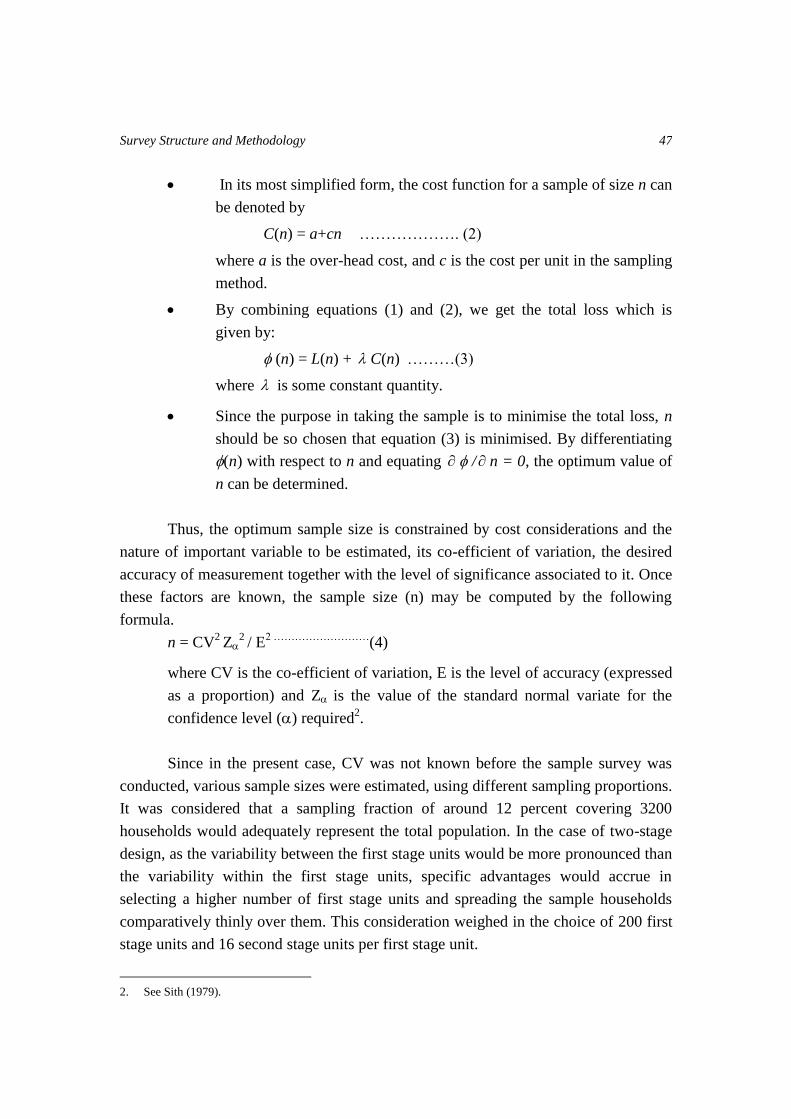
Survey Structure and Methodology
47
In its most simplified form, the cost function for a sample of size n can
be denoted by
C(n) = a+cn ………………. (2)
where a is the over-head cost, and c is the cost per unit in the sampling
method.
By combining equations (1) and (2), we get the total loss which is
given by:
(n) = L(n) + C(n) ………(3)
where is some constant quantity.
Since the purpose in taking the sample is to minimise the total loss, n
should be so chosen that equation (3) is minimised. By differentiating
(n) with respect to n and equating / n = 0, the optimum value of
n can be determined.
Thus, the optimum sample size is constrained by cost considerations and the
nature of important variable to be estimated, its co-efficient of variation, the desired
accuracy of measurement together with the level of significance associated to it. Once
these factors are known, the sample size (n) may be computed by the following
formula.
n = CV2
Z2
/ E2 ………………………
(4)
where CV is the co-efficient of variation, E is the level of accuracy (expressed
as a proportion) and Z is the value of the standard normal variate for the
confidence level () required2.
Since in the present case, CV was not known before the sample survey was
conducted, various sample sizes were estimated, using different sampling proportions.
It was considered that a sampling fraction of around 12 percent covering 3200
households would adequately represent the total population. In the case of two-stage
design, as the variability between the first stage units would be more pronounced than
the variability within the first stage units, specific advantages would accrue in
selecting a higher number of first stage units and spreading the sample households
comparatively thinly over them. This consideration weighed in the choice of 200 first
stage units and 16 second stage units per first stage unit.
2. See Sith (1979).

Socio-economic Impact of National Highway on Rural Population
48
Annex 3
List of sample villages
S. No. Census code 1991 Name of the village Block District State
1 210030008000150158 Dharmai Araon Firozabad Uttar Pradesh 2 210030008000160159 Sarai Haibatpur Araon Firozabad Uttar Pradesh 3 210030008000160162 Kithaut Araon Firozabad Uttar Pradesh 4 210030008000160163 Karahara Araon Firozabad Uttar Pradesh 5 210030008000170172 Shekhupur Araon Firozabad Uttar Pradesh 6 210010002000150135 Mondha Firozabad Firozabad Uttar Pradesh 7 210010002000160148 Jahangirpur Firozabad Firozabad Uttar Pradesh 8 210010002000160153 Nurpur Kutubpur Firozabad Firozabad Uttar Pradesh 9 210010002000170170 Matsena Firozabad Firozabad Uttar Pradesh
10 210030007000010005 Dargapur-Mohanipur Firozabad Firozabad Uttar Pradesh 11 210020005000140168 Lalai Khergarh Firozabad Uttar Pradesh 12 210020005000150175 Dhunpai Khergarh Firozabad Uttar Pradesh 13 210020005000160190 Keshopur Khergarh Firozabad Uttar Pradesh 14 210020005000160191 Prathavipur Khergarh Firozabad Uttar Pradesh 15 210020005000170207 Hasanpur Garia Khergarh Firozabad Uttar Pradesh 16 210030009000190199 Ujraikhera Madanpur Firozabad Uttar Pradesh 17 210030009000220223 Bithauli Madanpur Firozabad Uttar Pradesh 18 210030009000220227 Bachhmai Madanpur Firozabad Uttar Pradesh 19 210030009000220230 Naglator Madanpur Firozabad Uttar Pradesh 20 210030009000270272 Sujanipur Madanpur Firozabad Uttar Pradesh 21 210030009000280286 Semra Atikabad Madanpur Firozabad Uttar Pradesh 22 210030007000010002 Jinjauli Shikohabad Firozabad Uttar Pradesh 23 210030007000010004 Naoli Shikohabad Firozabad Uttar Pradesh 24 210030007000020014 Mohamdpur Labhna Shikohabad Firozabad Uttar Pradesh 25 210030007000020019 Dewaechi Shikohabad Firozabad Uttar Pradesh 26 210030007000020024 Maiyamai Shikohabad Firozabad Uttar Pradesh 27 210030007000020026 Shaijalpur Shikohabad Firozabad Uttar Pradesh 28 210030007000030030 Basudeomai Shikohabad Firozabad Uttar Pradesh 29 210030007000030032 Nagla Saidlal Shikohabad Firozabad Uttar Pradesh 30 210030007000040046 Bakalpur Shikohabad Firozabad Uttar Pradesh 31 210030007000050050 Jaslai Shikohabad Firozabad Uttar Pradesh 32 210030007000050053 Mohabatpur Ahir Shikohabad Firozabad Uttar Pradesh 33 210030007000050056 Jahagirpur Gulrai Shikohabad Firozabad Uttar Pradesh 34 210030007000010001 Makhanpur Sikohabad Firozabad Uttar Pradesh 35 210010002000170163 Undani Friozabad Friozabad Uttar Pradesh 36 350040012000100074 Ailchipur Ajitmal Auraiya Uttar Pradesh 37 350040012000110086 Shekhupur Jainpur Ajitmal Auraiya Uttar Pradesh 38 350040012000120093 Bahadurpur Uncha Ajitmal Auraiya Uttar Pradesh 39 350040012000130106 Purwadori Ajitmal Auraiya Uttar Pradesh 40 350040012000130109 Jagatpur Ajitmal Auraiya Uttar Pradesh 41 350040012000130110 Turkipur Bhagwandas Ajitmal Auraiya Uttar Pradesh 42 350040014000310275 Akbarpur Auraiya Auraiya Uttar Pradesh 43 350040014000350316 Takpura Auraiya Auraiya Uttar Pradesh 44 350040014000360324 Hasuliya Auraiya Auraiya Uttar Pradesh 45 350040014000370332 Parariya Auraiya Auraiya Uttar Pradesh 46 350040014000370333 Garha Manik Chandra Auraiya Auraiya Uttar Pradesh 47 350040014000370334 Salaiya Auraiya Auraiya Uttar Pradesh 48 350040014000380342 Tilakpur Auraiya Auraiya Uttar Pradesh 49 350040014000380344 Inguthiya Auraiya Auraiya Uttar Pradesh
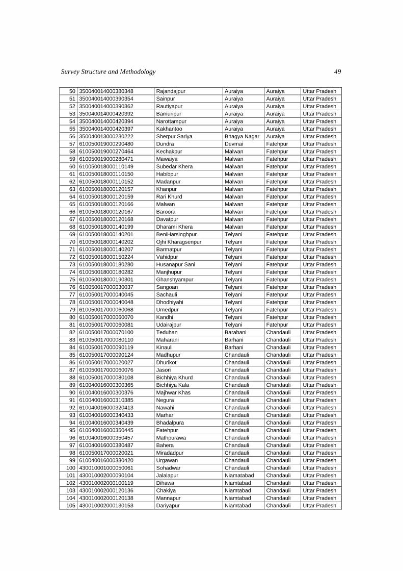
Survey Structure and Methodology
49
50 350040014000380348 Rajandajpur Auraiya Auraiya Uttar Pradesh 51 350040014000390354 Sainpur Auraiya Auraiya Uttar Pradesh 52 350040014000390362 Rautiyapur Auraiya Auraiya Uttar Pradesh 53 350040014000420392 Bamuripur Auraiya Auraiya Uttar Pradesh 54 350040014000420394 Narottampur Auraiya Auraiya Uttar Pradesh 55 350040014000420397 Kakhantoo Auraiya Auraiya Uttar Pradesh 56 350040013000230222 Sherpur Sariya Bhagya Nagar Auraiya Uttar Pradesh 57 610050019000290480 Dundra Devmai Fatehpur Uttar Pradesh 58 610050019000270464 Kechakpur Malwan Fatehpur Uttar Pradesh 59 610050019000280471 Mawaiya Malwan Fatehpur Uttar Pradesh 60 610050018000110149 Subedar Khera Malwan Fatehpur Uttar Pradesh 61 610050018000110150 Habibpur Malwan Fatehpur Uttar Pradesh 62 610050018000110152 Madanpur Malwan Fatehpur Uttar Pradesh 63 610050018000120157 Khanpur Malwan Fatehpur Uttar Pradesh 64 610050018000120159 Rari Khurd Malwan Fatehpur Uttar Pradesh 65 610050018000120166 Malwan Malwan Fatehpur Uttar Pradesh 66 610050018000120167 Baroora Malwan Fatehpur Uttar Pradesh 67 610050018000120168 Davatpur Malwan Fatehpur Uttar Pradesh 68 610050018000140199 Dharami Khera Malwan Fatehpur Uttar Pradesh 69 610050018000140201 BeniHarsinghpur Telyani Fatehpur Uttar Pradesh 70 610050018000140202 Ojhi Kharagsenpur Telyani Fatehpur Uttar Pradesh 71 610050018000140207 Barmatpur Telyani Fatehpur Uttar Pradesh 72 610050018000150224 Vahidpur Telyani Fatehpur Uttar Pradesh 73 610050018000180280 Husanapur Sani Telyani Fatehpur Uttar Pradesh 74 610050018000180282 Manjhupur Telyani Fatehpur Uttar Pradesh 75 610050018000190301 Ghanshyampur Telyani Fatehpur Uttar Pradesh 76 610050017000030037 Sangoan Telyani Fatehpur Uttar Pradesh 77 610050017000040045 Sachauli Telyani Fatehpur Uttar Pradesh 78 610050017000040048 Dhodhiyahi Telyani Fatehpur Uttar Pradesh 79 610050017000060068 Umedpur Telyani Fatehpur Uttar Pradesh 80 610050017000060070 Kandhi Telyani Fatehpur Uttar Pradesh 81 610050017000060081 Udairajpur Telyani Fatehpur Uttar Pradesh 82 610050017000070100 Teduhan Barahani Chandauli Uttar Pradesh 83 610050017000080110 Maharani Barhani Chandauli Uttar Pradesh 84 610050017000090119 Kinauli Barhani Chandauli Uttar Pradesh 85 610050017000090124 Madhupur Chandauli Chandauli Uttar Pradesh 86 610050017000020027 Dhurikot Chandauli Chandauli Uttar Pradesh 87 610050017000060076 Jasori Chandauli Chandauli Uttar Pradesh 88 610050017000080108 Bichhiya Khurd Chandauli Chandauli Uttar Pradesh 89 610040016000300365 Bichhiya Kala Chandauli Chandauli Uttar Pradesh 90 610040016000300376 Majhwar Khas Chandauli Chandauli Uttar Pradesh 91 610040016000310385 Negura Chandauli Chandauli Uttar Pradesh 92 610040016000320413 Nawahi Chandauli Chandauli Uttar Pradesh 93 610040016000340433 Marhar Chandauli Chandauli Uttar Pradesh 94 610040016000340439 Bhadalpura Chandauli Chandauli Uttar Pradesh 95 610040016000350445 Fatehpur Chandauli Chandauli Uttar Pradesh 96 610040016000350457 Mathpurawa Chandauli Chandauli Uttar Pradesh 97 610040016000380487 Bahera Chandauli Chandauli Uttar Pradesh 98 610050017000020021 Miradadpur Chandauli Chandauli Uttar Pradesh 99 610040016000330420 Urgawan Chandauli Chandauli Uttar Pradesh
100 430010001000050061 Sohadwar Chandauli Chandauli Uttar Pradesh 101 430010002000090104 Jalalapur Niamatabad Chandauli Uttar Pradesh 102 430010002000100119 Dihawa Niamtabad Chandauli Uttar Pradesh 103 430010002000120136 Chakiya Niamtabad Chandauli Uttar Pradesh 104 430010002000120138 Mannapur Niamtabad Chandauli Uttar Pradesh 105 430010002000130153 Dariyapur Niamtabad Chandauli Uttar Pradesh
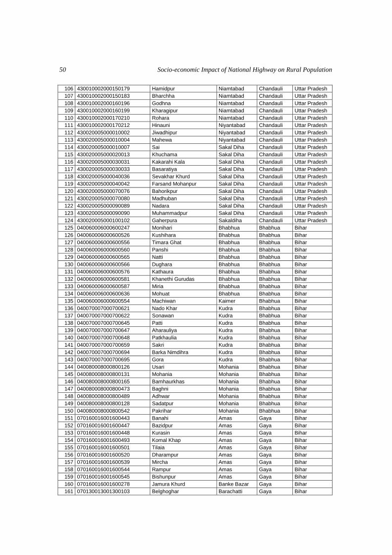
Socio-economic Impact of National Highway on Rural Population
50
106 430010002000150179 Hamidpur Niamtabad Chandauli Uttar Pradesh 107 430010002000150183 Bharchha Niamtabad Chandauli Uttar Pradesh 108 430010002000160196 Godhna Niamtabad Chandauli Uttar Pradesh 109 430010002000160199 Kharagipur Niamtabad Chandauli Uttar Pradesh 110 430010002000170210 Rohara Niamtabad Chandauli Uttar Pradesh 111 430010002000170212 Hinauni Niyantabad Chandauli Uttar Pradesh 112 430020005000010002 Jiwadhipur Niyantabad Chandauli Uttar Pradesh 113 430020005000010004 Mahewa Niyantabad Chandauli Uttar Pradesh 114 430020005000010007 Sai Sakal Diha Chandauli Uttar Pradesh 115 430020005000020013 Khuchama Sakal Diha Chandauli Uttar Pradesh 116 430020005000030031 Kakarahi Kala Sakal Diha Chandauli Uttar Pradesh 117 430020005000030033 Basaratiya Sakal Diha Chandauli Uttar Pradesh 118 430020005000040036 Sevakhar Khurd Sakal Diha Chandauli Uttar Pradesh 119 430020005000040042 Farsand Mohanpur Sakal Diha Chandauli Uttar Pradesh 120 430020005000070076 Bahorikpur Sakal Diha Chandauli Uttar Pradesh 121 430020005000070080 Madhuban Sakal Diha Chandauli Uttar Pradesh 122 430020005000090089 Nadara Sakal Diha Chandauli Uttar Pradesh 123 430020005000090090 Muhammadpur Sakal Diha Chandauli Uttar Pradesh 124 430020005000100102 Gaherpura Sakaldiha Chandauli Uttar Pradesh
125 040060006000600247 Monihari Bhabhua Bhabhua Bihar
126 040060006000600526 Kushihara Bhabhua Bhabhua Bihar
127 040060006000600556 Timara Ghat Bhabhua Bhabhua Bihar
128 040060006000600560 Panshi Bhabhua Bhabhua Bihar
129 040060006000600565 Natti Bhabhua Bhabhua Bihar
130 040060006000600566 Dughara Bhabhua Bhabhua Bihar
131 040060006000600576 Kathaura Bhabhua Bhabhua Bihar
132 040060006000600581 Khanethi Gurudas Bhabhua Bhabhua Bihar
133 040060006000600587 Miria Bhabhua Bhabhua Bihar
134 040060006000600636 Mohuat Bhabhua Bhabhua Bihar
135 040060006000600554 Machiwan Kaimer Bhabhua Bihar
136 040070007000700621 Nado Khar Kudra Bhabhua Bihar
137 040070007000700622 Sonawan Kudra Bhabhua Bihar
138 040070007000700645 Patti Kudra Bhabhua Bihar
139 040070007000700647 Aharauliya Kudra Bhabhua Bihar
140 040070007000700648 Patkhaulia Kudra Bhabhua Bihar
141 040070007000700659 Sakri Kudra Bhabhua Bihar
142 040070007000700694 Barka Nimdihra Kudra Bhabhua Bihar
143 040070007000700695 Gora Kudra Bhabhua Bihar
144 040080008000800126 Usari Mohania Bhabhua Bihar
145 040080008000800131 Mohania Mohania Bhabhua Bihar
146 040080008000800165 Bamhaurkhas Mohania Bhabhua Bihar
147 040080008000800473 Baghni Mohania Bhabhua Bihar
148 040080008000800489 Adhwar Mohania Bhabhua Bihar
149 040080008000800128 Sadatpur Mohania Bhabhua Bihar
150 040080008000800542 Pakrihar Mohania Bhabhua Bihar
151 070160016001600443 Banahi Amas Gaya Bihar
152 070160016001600447 Bazidpur Amas Gaya Bihar
153 070160016001600448 Kurasin Amas Gaya Bihar
154 070160016001600493 Komal Khap Amas Gaya Bihar
155 070160016001600501 Tilaia Amas Gaya Bihar
156 070160016001600520 Dharampur Amas Gaya Bihar
157 070160016001600539 Mircha Amas Gaya Bihar
158 070160016001600544 Rampur Amas Gaya Bihar
159 070160016001600545 Bishunpur Amas Gaya Bihar
160 070160016001600278 Jamura Khurd Banke Bazar Gaya Bihar
161 070130013001300103 Belghoghar Barachatti Gaya Bihar

Survey Structure and Methodology
51
162 070130013001300108 Manjhuali Barachatti Gaya Bihar
163 070130013001300130 Makhdumpur Barachatti Gaya Bihar
164 070130013001300139 Sonbarsa Barachatti Gaya Bihar
165 070130013001300146 Dharamthan Barachatti Gaya Bihar
166 070130013001300173 Kalua Khurd Barachatti Gaya Bihar
167 070130013001300180 Rohi Barachatti Gaya Bihar
168 070130013001300181 Bhaghar Barachatti Gaya Bihar
169 070130013001300184 Mankumhari Barachatti Gaya Bihar
170 070130013001300185 Bhat Bigha Barachatti Gaya Bihar
171 070130013001300144 Jodha Bigha Dobhi Gaya Bihar
172 070130013001300156 Bundabigha Dobhi Gaya Bihar
173 070130013001300159 Kaleyanpur Dobhi Gaya Bihar
174 070130013001300168 Mushehani Dobhi Gaya Bihar
175 070130013001300201 Kurmawan Dobhi Gaya Bihar
176 070130013001300212 Gangi Dobhi Gaya Bihar
177 070140014001400781 Ghorwadih Dobhi Gaya Bihar
178 070140014001400787 Darioaura Dobhi Gaya Bihar
179 070140014001400805 Wari Dobhi Gaya Bihar
180 070140014001400837 Marha Dobhi Gaya Bihar
181 070150015001500500 Morahar Gurva Gaya Bihar
182 070150015001500578 Hasanpur Gurva Gaya Bihar
183 070150015001500599 Pakari Gurva Gaya Bihar
184 070140014001400418 Bhikhanpur Sherghati Gaya Bihar
185 070140014001400749 Kalendara Sherghati Gaya Bihar
186 070140014001400756 Majhanpur Sherghati Gaya Bihar
187 070140014001400773 Bhus Bhusia Sherghati Gaya Bihar
188 340160016001600167 Ranichunwa Burhi Hazaribagh Jharkhand
189 340160016001600142 Pipra Ghoghar Barhani Hazaribagh Jharkhand
190 340160016001600166 Mahugarha Barhani Hazaribagh Jharkhand
191 340160016001600072 Konra Burhi Hazaribagh Jharkhand
192 340160016001600136 Malkoko Burhi Hazaribagh Jharkhand
193 340040004000400050 Tuio Barkatha Hazaribagh Jharkhand
194 340040004000400053 Buchai Pathauria Barkatha Hazaribagh Jharkhand
195 340040004000400079 Jhurjhuri Barkatha Hazaribagh Jharkhand
196 340040004000400103 Masipirhi Barkatha Hazaribagh Jharkhand
197 340040004000400096 Ghanghari Barkatha Hazaribagh Jharkhand
198 340040004000400109 Lemua Barkatha Hazaribagh Jharkhand
199 340040004000400118 Dumardiha Barkatha Hazaribagh Jharkhand
200 340160016001600123 Karma Burhi Hazaribagh Jharkhand
Chapter 3
Socio-economic Profile of Rural Households
This chapter provides an overview of the temporal changes in some
aggregative indicators of socio-economic development between pre- and post-
upgrading of NH2 for rural households living in different districts falling in the
selected stretches around the highway as revealed by the baseline and the resurvey
data sets. These indicators, relating to demography, mobility, poverty, sector
composition of household income and employment, ownership of assets, etc., should
reflect the state or stage of development of the economy of an area. Therefore, their
temporal changes, should tell us about the qualitative improvement, if any, between
the time points concerned. As such, many of these indicators are essentially socio-
economic parameters in the sense that their values may improve over long period with
income development unless very strong and effective specific public policy
interventions are made. Since the time-gap between the two surveys is seven years
and not long, any observed improvement in indicators may partly be ascribed to the
NH2 upgrading.
The Table 0 below gives the list of indicators used in the present analysis. It
may be noted that there are 18 indicators, of which 4 are examined separately for
female population to see the presence of a significant gender-specific pattern, if any,
and for one the patterns for scheduled caste and scheduled tribe population have also
been examined. In each case, temporal change has been examined separately for the
sample of poor and non-poor households as well as for the pooled sample of
households. In what follows, for every indicator, a table giving baseline and resurvey
values of the indicator by stretch (district) for the poor, the non-poor and the
aggregate sample of households and figure(s) showing corresponding baseline and
resurvey graphs are presented and discussed. The graphs have the stretches (districts)
shown along the horizontal axis (arranged in order of their position on NH2 as one
moves along the highway from NW to SE) and the indicator value on the vertical axis.
Also, the baseline and resurvey graphs are shown on the same figure to facilitate a
visual inspection of the temporal shifts. Needless to mention, this analysis should also
help to ascertain if any positive impact of NH2 upgrading has been progressive and
socially inclusive.
Socio-economic Profile of Rural Households 53
Table 0: List of selected Indicators of socio-economic development used
Nature of indicator Indicators examined
Socio-demographic 1. Household size 2. Sex ratio 3. Dependency ratio 4. Literacy rate 5. School enrolment rate
Health 6. Proportion of Households visiting a doctor
Expenditure pattern 7. Share of food, education and health in total consumer expenditure
Mobility 8. Per capita weekly trip rate 9. Per capita weekly trip length
Poverty 10. Percentage of poor households 11. Percentage of poor persons
Asset ownership and income composition
12. Land holding per household 13. No. of consumer durables owned per household 14. Share of income from agriculture
Employment 15. Proportion of working population 16. Proportion of working population engaged in non-
agriculture
Household size
Socio-economic development affects the household size in two ways. At the
first stage of development, generally there is an increase in the household size via the
decline in the mortality rate compared to the fertility rate and, at an advanced stage of
development, the household size decreases due to decline in the fertility rate as well.
The average household size in the states of Bihar and Uttar Pradesh has
generally been higher than the national average size. In the census of 2001, while the
national average was 5.3, the same was 6.4 for Uttar Pradesh and 6 for Bihar1. In the
stretches selected on the basis of high incidence of poverty, the average household
size worked out to 6.5 for Uttar Pradesh and as high as 7.6 for Bihar and Jharkhand.
The poor households have a still higher size as compared to the non-poor. Indeed, in
their case, the growth rate has been much higher in Bihar and Jharkhand.
Table 1: Average household size (number of family members)
Stretch Aggregate Poor Non-poor
Baseline Resurvey Baseline Resurvey Baseline Resurvey
Firozabad 6.1 6.6 6.6 6.8 5.8 6.5
Auraiya 5.5 6.3 6.7 7.5 5.1 5.3
Fatehpur 5.5 6.1 6.3 6.7 5.3 5.8
Chandauli 6.5 6.7 6.5 7.0 6.5 6.6
Bhabhua 7.2 8.0 6.5 8.1 7.7 7.9
Gaya 6.8 7.4 7.0 7.8 6.5 6.9
Hazaribagh 7.0 7.4 7.1 8.0 6.6 6.8
Uttar Pradesh 6.0 6.5 6.6 7.0 5.8 6.2
Bihar and Jharkhand 7.0 7.6 6.9 8.0 7.0 7.2
Total 6.4 6.9 6.7 7.4 6.2 6.6
1. As per the labour bureau survey the average rural household size is 5.8 for Bihar, 5.3 for Jharkhand and 5.9
for Uttar Pradesh. Government of India, 2010. “Report on Employment and Unemployment Survey (2009-
10)”, Ministry of Labour & Employment, New Delhi.

Socio-economic Impact of National Highway on Rural Population 54
Figure 1(a): Average household size (aggregate)
Figure 1(b): Average household size among the poor
Average household size (poor)
Average household size (non-poor)
Figure 1(c): Average household size among the non-poor
Sex ratio
The sex ratio of population is one of the major indicators of the gender related
status of development. The higher status and empowerment of women is expected to
rise with development, as higher income gives wider opportunities and freedom to
make choices. This gets reflected in the level of care a girl child receives and whether
any pre-natal gender determination and foeticide takes place or not2.
2. Dreze and Murthi (2001) argue that the increase in female foeticide is directly a reason of technological
diffusion. One may argue that as the access to roads have improved; households have also gained access to
quack clinics which offer pre-natal sex determination, earlier not available within the village.
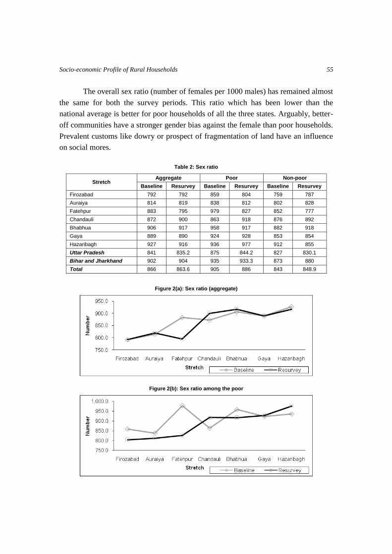
Socio-economic Profile of Rural Households 55
The overall sex ratio (number of females per 1000 males) has remained almost
the same for both the survey periods. This ratio which has been lower than the
national average is better for poor households of all the three states. Arguably, better-
off communities have a stronger gender bias against the female than poor households.
Prevalent customs like dowry or prospect of fragmentation of land have an influence
on social mores.
Table 2: Sex ratio
Stretch Aggregate Poor Non-poor
Baseline Resurvey Baseline Resurvey Baseline Resurvey
Firozabad 792 792 859 804 759 787
Auraiya 814 819 838 812 802 828
Fatehpur 883 795 979 827 852 777
Chandauli 872 900 863 918 876 892
Bhabhua 906 917 958 917 882 918
Gaya 889 890 924 928 853 854
Hazaribagh 927 916 936 977 912 855
Uttar Pradesh 841 835.2 875 844.2 827 830.1
Bihar and Jharkhand 902 904 935 933.3 873 880
Total 866 863.6 905 886 843 848.9
Figure 2(a): Sex ratio (aggregate)
Figure 2(b): Sex ratio among the poor
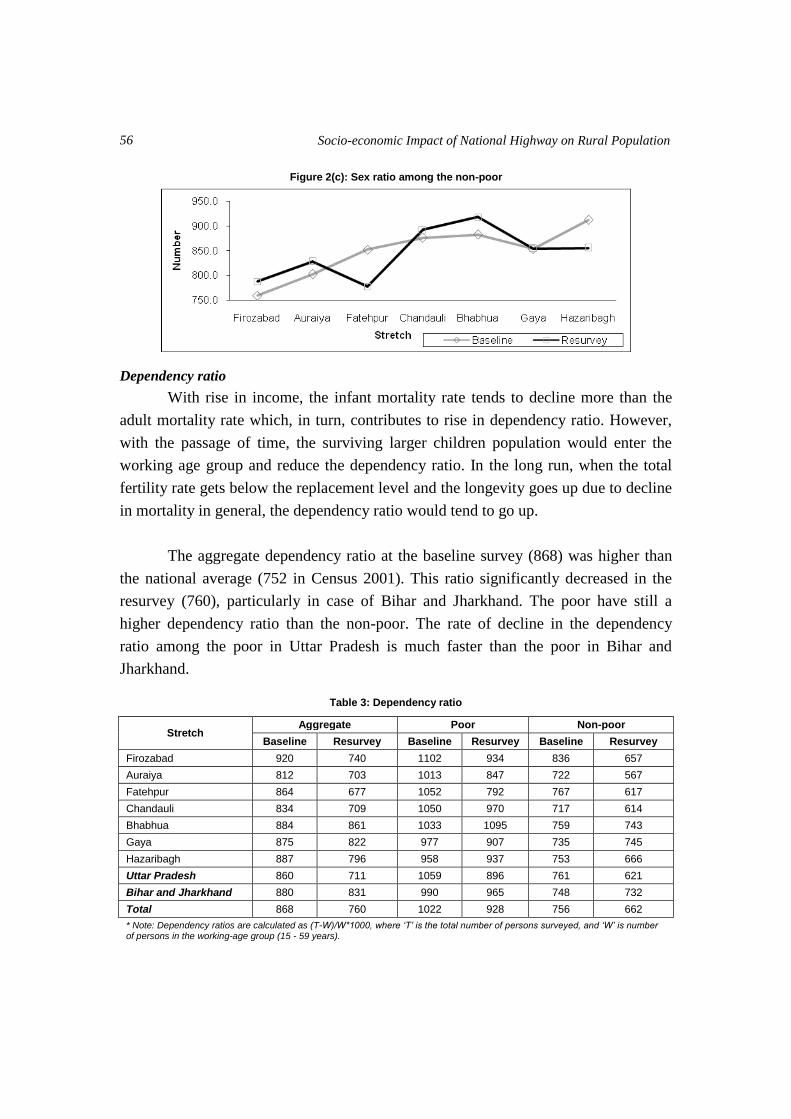
Socio-economic Impact of National Highway on Rural Population 56
Figure 2(c): Sex ratio among the non-poor
Dependency ratio
With rise in income, the infant mortality rate tends to decline more than the
adult mortality rate which, in turn, contributes to rise in dependency ratio. However,
with the passage of time, the surviving larger children population would enter the
working age group and reduce the dependency ratio. In the long run, when the total
fertility rate gets below the replacement level and the longevity goes up due to decline
in mortality in general, the dependency ratio would tend to go up.
The aggregate dependency ratio at the baseline survey (868) was higher than
the national average (752 in Census 2001). This ratio significantly decreased in the
resurvey (760), particularly in case of Bihar and Jharkhand. The poor have still a
higher dependency ratio than the non-poor. The rate of decline in the dependency
ratio among the poor in Uttar Pradesh is much faster than the poor in Bihar and
Jharkhand.
Table 3: Dependency ratio
Stretch Aggregate Poor Non-poor
Baseline Resurvey Baseline Resurvey Baseline Resurvey
Firozabad 920 740 1102 934 836 657
Auraiya 812 703 1013 847 722 567
Fatehpur 864 677 1052 792 767 617
Chandauli 834 709 1050 970 717 614
Bhabhua 884 861 1033 1095 759 743
Gaya 875 822 977 907 735 745
Hazaribagh 887 796 958 937 753 666
Uttar Pradesh 860 711 1059 896 761 621
Bihar and Jharkhand 880 831 990 965 748 732
Total 868 760 1022 928 756 662
* Note: Dependency ratios are calculated as (T-W)/W*1000, where ‘T’ is the total number of persons surveyed, and ‘W’ is number of persons in the working-age group (15 - 59 years).

Socio-economic Profile of Rural Households 57
Figure 3(a): Dependency ratio (aggregate)
Figure 3(b): Dependency ratio among the poor
Figure 3(c): Dependency ratio among the non-poor
Literacy level
The persistence of widespread illiteracy among the disadvantaged groups
tends to reinforce diverse kinds of social inequality. The expansion of basic education,
thus, is seen as an essential requirement for rapid elimination of these inequalities,
and for positive social change. Thus, literacy level is one of the most important
indicators of human development and a vital determinant of human capabilities.
The overall literacy level (61.86 percent) has improved across all the stretches,
but it is still lower than the national average of 65.38 percent (Census 2001).
Socio-economic Impact of National Highway on Rural Population 58
However, inter-state and class differences still persist. In case of the poor households,
literacy attainment is 17 percent less as compared to the non-poor households.
Literacy level has gone down among the poor in Bihar and Jharkhand as compared to
Uttar Pradesh. In contrast, among the non-poor, literacy level has improved in Bihar
& Jharkhand as compared to Uttar Pradesh.
Table 4: Literacy level (percent)
Stretch Aggregate Poor Non-poor
Baseline Resurvey Baseline Resurvey Baseline Resurvey
Firozabad 58.36 66.58 53.28 59.95 61.04 69.91
Auraiya 62.55 72.03 61.83 68.03 62.93 76.49
Fatehpur 55.51 67.32 61.70 60.96 51.78 70.97
Chandauli 60.85 64.98 60.85 50.47 60.85 71.43
Bhabhua 58.91 60.60 65.26 46.35 52.72 69.26
Gaya 45.00 51.40 45.33 42.31 44.47 60.36
Hazaribagh 46.31 51.98 47.40 46.55 44.02 57.80
Uttar Pradesh 59.42 67.00 59.13 59.07 59.59 71.48
Bihar and Jharkhand 50.18 54.81 51.78 44.31 47.96 63.65
Total 55.58 61.86 55.25 51.98 55.86 68.48
Figure 4(a): Literacy level (aggregate)
Figure 4(b): Literacy level among the poor

Socio-economic Profile of Rural Households 59
Figure 4(c): Literacy level among the non-poor
Female literacy level
Women's education has been consistently viewed not only as a benefit in
itself, but as a means of achieving other development goals. The women’s status and
gender-related state of development is also reflected in the female literacy level and
school enrolment of girls which are the fundamental factors for the development of
women’s awareness and their capability.
Census 2001 registered 54.16 percent female literacy. For the selected
stretches, female literacy has shown considerable improvement, though it is still
below the overall literacy level (male and female aggregate). The disparity between
the poor and non-poor households persists. Female literacy rate among the poor
households is increasing at a much faster rate than the non-poor households.
Table 5: Female literacy (percent)
Stretch Aggregate Poor Non-poor
Baseline Resurvey Baseline Resurvey Baseline Resurvey
Firozabad 38.19 56.39 31.57 50.95 41.63 59.15
Auraiya 48.20 66.10 44.24 62.04 50.00 70.57
Fatehpur 39.17 57.93 30.50 52.91 41.96 60.91
Chandauli 44.56 54.23 30.89 39.36 49.39 60.93
Bhabhua 46.08 51.17 30.00 36.19 53.37 60.27
Gaya 32.12 41.47 24.51 33.43 40.05 49.75
Hazaribagh 26.55 39.66 24.71 36.58 29.52 43.20
Uttar Pradesh 42.37 57.38 33.33 50.07 46.03 61.54
Bihar and Jharkhand 36.08 44.69 25.87 34.85 44.74 53.23
Total 39.73 51.89 29.34 42.55 45.57 58.30
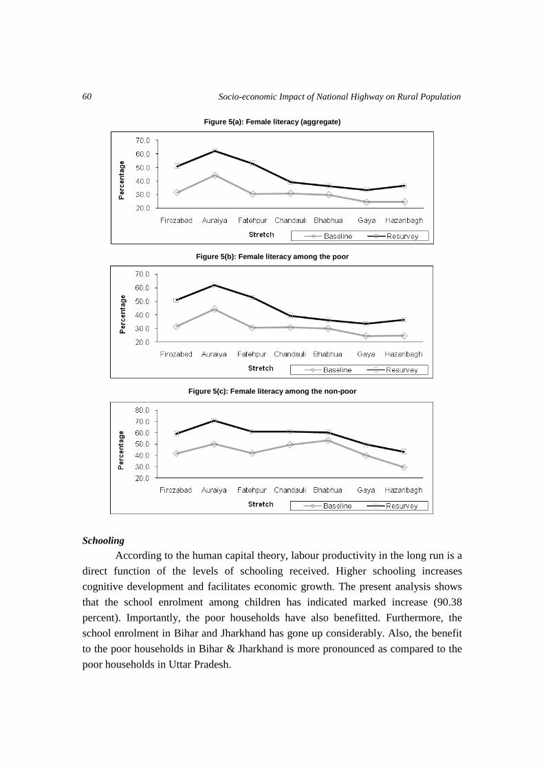
Socio-economic Impact of National Highway on Rural Population 60
Figure 5(a): Female literacy (aggregate)
Figure 5(b): Female literacy among the poor
Figure 5(c): Female literacy among the non-poor
Schooling
According to the human capital theory, labour productivity in the long run is a
direct function of the levels of schooling received. Higher schooling increases
cognitive development and facilitates economic growth. The present analysis shows
that the school enrolment among children has indicated marked increase (90.38
percent). Importantly, the poor households have also benefitted. Furthermore, the
school enrolment in Bihar and Jharkhand has gone up considerably. Also, the benefit
to the poor households in Bihar & Jharkhand is more pronounced as compared to the
poor households in Uttar Pradesh.
Socio-economic Profile of Rural Households 61
Table 6: School enrolment (percent)
Stretch Aggregate Poor Non-poor
Baseline Resurvey Baseline Resurvey Baseline Resurvey
Firozabad 84.30 91.17 78.82 86.69 87.91 94.18
Auraiya 94.19 93.64 93.29 93.91 94.74 93.30
Fatehpur 91.47 89.16 91.12 83.98 91.72 92.81
Chandauli 88.42 91.14 81.09 84.95 93.55 94.40
Bhabhua 85.82 92.57 79.11 87.46 93.75 96.11
Gaya 68.32 86.97 61.71 81.53 80.37 92.75
Hazaribagh 76.02 89.13 72.88 84.95 83.02 94.85
Uttar Pradesh 88.67 91.16 84.14 87.20 91.75 93.91
Bihar and Jharkhand 75.77 89.35 69.24 83.99 86.32 94.43
Total 83.40 90.38 76.50 85.67 90.08 94.12
Figure 6(a): School enrolment (aggregate)
Figure 6(b): School enrolment among children of the poor
Figure 6(c): School enrolment among children of the non-poor

Socio-economic Impact of National Highway on Rural Population 62
Schooling among girls
The individual and social returns from the women’s education are believed to
be exceptionally high especially where the lowering of fertility and infant and child
mortality rate are concerned. In addition, rising levels of education of women lead to
improvement in nutrition and healthcare facilities as also in the children’s educational
achievements. Prejudice against the education of girls has a strong detrimental effect
on the amount of schooling they receive. Resurvey data shows a significant rise in
school enrolment among girls particularly in the states of Bihar and Jharkhand.
Importantly, there is also marked improvement in this regard in the case of poor
households. On an aggregate, 90 percent of the girl children attend school; 84 percent
even in the poor families. These are positive developments reflecting the awareness of
the society towards the care of a girl child.
Table 7: Percentage of female school going children
Stretch Aggregate Poor Non-poor
Baseline Resurvey Baseline Resurvey Baseline Resurvey
Firozabad 77.88 89.63 72.66 83.89 81.68 93.94
Auraiya 93.88 95.70 93.94 94.64 93.85 97.30
Fatehpur 88.03 89.73 87.38 83.33 88.55 94.53
Chandauli 85.29 92.57 80.42 85.03 88.57 96.30
Bhabhua 78.34 90.36 70.52 82.27 87.94 95.50
Gaya 62.53 85.68 54.98 79.59 75.64 92.82
Hazaribagh 70.76 89.70 64.35 85.15 83.93 96.88
Uttar Pradesh 85.19 91.67 81.49 86.51 87.70 95.41
Bihar and Jharkhand 69.52 88.09 63.05 81.52 81.87 94.55
Total 78.51 90.06 71.02 84.06 85.81 95.05
Figure 7(a): Female school-going children (aggregate)
Female school-going children (poor)
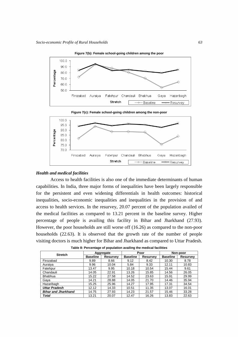
Socio-economic Profile of Rural Households 63
Figure 7(b): Female school-going children among the poor
Figure 7(c): Female school-going children among the non-poor
Health and medical facilities
Access to health facilities is also one of the immediate determinants of human
capabilities. In India, three major forms of inequalities have been largely responsible
for the persistent and even widening differentials in health outcomes: historical
inequalities, socio-economic inequalities and inequalities in the provision of and
access to health services. In the resurvey, 20.07 percent of the population availed of
the medical facilities as compared to 13.21 percent in the baseline survey. Higher
percentage of people is availing this facility in Bihar and Jharkhand (27.93).
However, the poor households are still worse off (16.26) as compared to the non-poor
households (22.63). It is observed that the growth rate of the number of people
visiting doctors is much higher for Bihar and Jharkhand as compared to Uttar Pradesh.
Table 8: Percentage of population availing the medical facilities
Stretch Aggregate Poor Non-poor
Baseline Resurvey Baseline Resurvey Baseline Resurvey
Firozabad 9.89 8.66 9.12 8.42 10.30 8.78
Auraiya 9.96 10.04 5.84 9.33 12.11 10.83
Fatehpur 13.47 9.95 10.18 10.54 15.44 9.61
Chandauli 14.05 22.91 13.26 15.85 14.56 26.05
Bhabhua 15.22 27.58 14.52 23.63 15.91 29.99
Gaya 14.21 28.88 14.05 21.70 14.46 35.94
Hazaribagh 15.25 25.96 14.27 17.95 17.31 34.54
Uttar Pradesh 12.12 14.33 10.51 11.35 13.07 16.01
Bihar and Jharkhand 14.75 27.93 14.23 21.57 15.46 33.28
Total 13.21 20.07 12.47 16.26 13.83 22.63

Socio-economic Impact of National Highway on Rural Population 64
Figure 8(a): Percentage of population availing the medical facilities (aggregate)
Figure 8(b): Percentage of population availing the medical facilities among the poor
Figure 8(c): Percentage of population availing the medical facilities among the non-poor
Expenditure patterns
Economists perceive the share of food in total expenditure as an indicator of
the level of consumption and the standard of living. A higher value suggests that
households are mostly spending on necessities, being nearer the subsistence level,
and, as such, are at a lower level of well-being.
Generally, poor people have to spend larger portion of their income on food,
estimated to be about 75 percent. For the non-poor households, it is less than half of
it. There are, however, spatial differences in expenditure patterns. The growth rate of
share of expenditure on food is much higher for Bihar and Jharkhand, and
surprisingly, for the non-poor households.
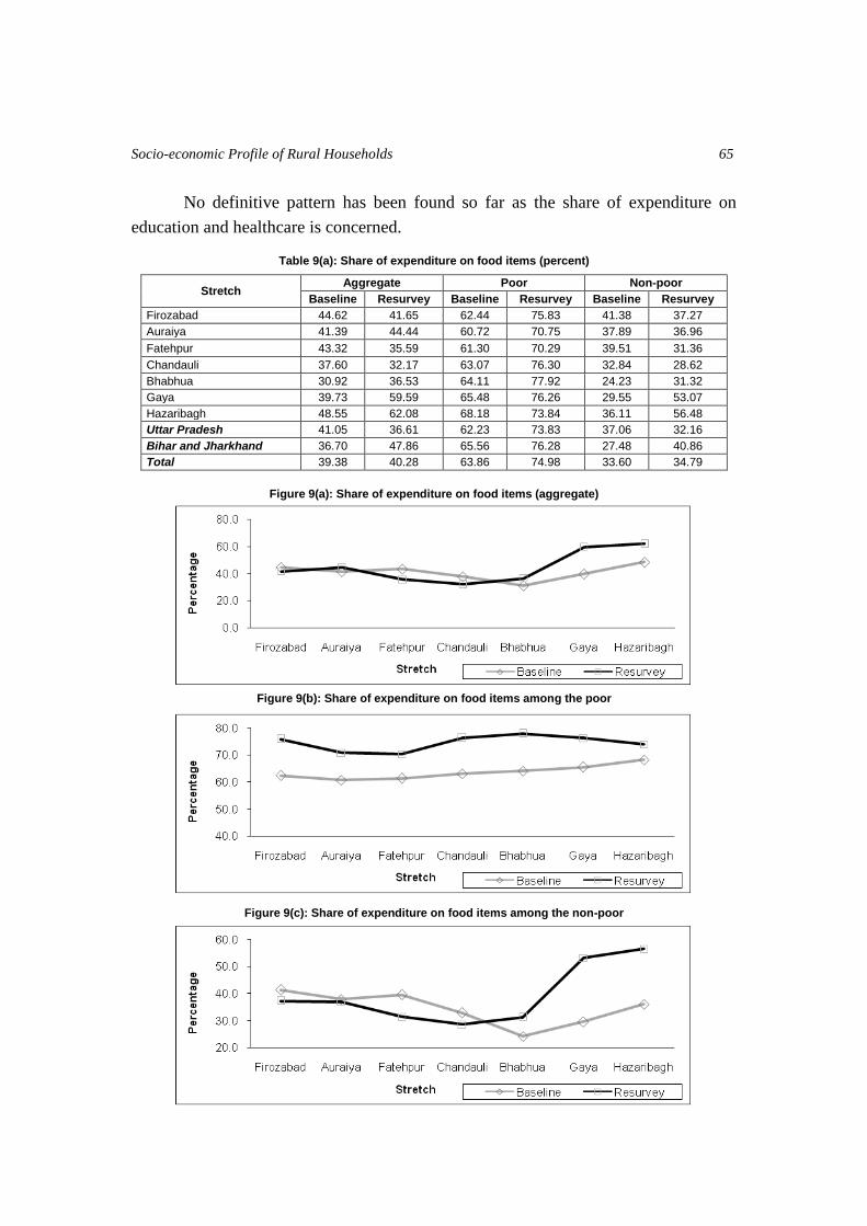
Socio-economic Profile of Rural Households 65
No definitive pattern has been found so far as the share of expenditure on
education and healthcare is concerned.
Table 9(a): Share of expenditure on food items (percent)
Stretch Aggregate Poor Non-poor
Baseline Resurvey Baseline Resurvey Baseline Resurvey
Firozabad 44.62 41.65 62.44 75.83 41.38 37.27
Auraiya 41.39 44.44 60.72 70.75 37.89 36.96
Fatehpur 43.32 35.59 61.30 70.29 39.51 31.36
Chandauli 37.60 32.17 63.07 76.30 32.84 28.62
Bhabhua 30.92 36.53 64.11 77.92 24.23 31.32
Gaya 39.73 59.59 65.48 76.26 29.55 53.07
Hazaribagh 48.55 62.08 68.18 73.84 36.11 56.48
Uttar Pradesh 41.05 36.61 62.23 73.83 37.06 32.16
Bihar and Jharkhand 36.70 47.86 65.56 76.28 27.48 40.86
Total 39.38 40.28 63.86 74.98 33.60 34.79
Figure 9(a): Share of expenditure on food items (aggregate)
Figure 9(b): Share of expenditure on food items among the poor
Figure 9(c): Share of expenditure on food items among the non-poor
Table 9(b): Share of expenditure on education
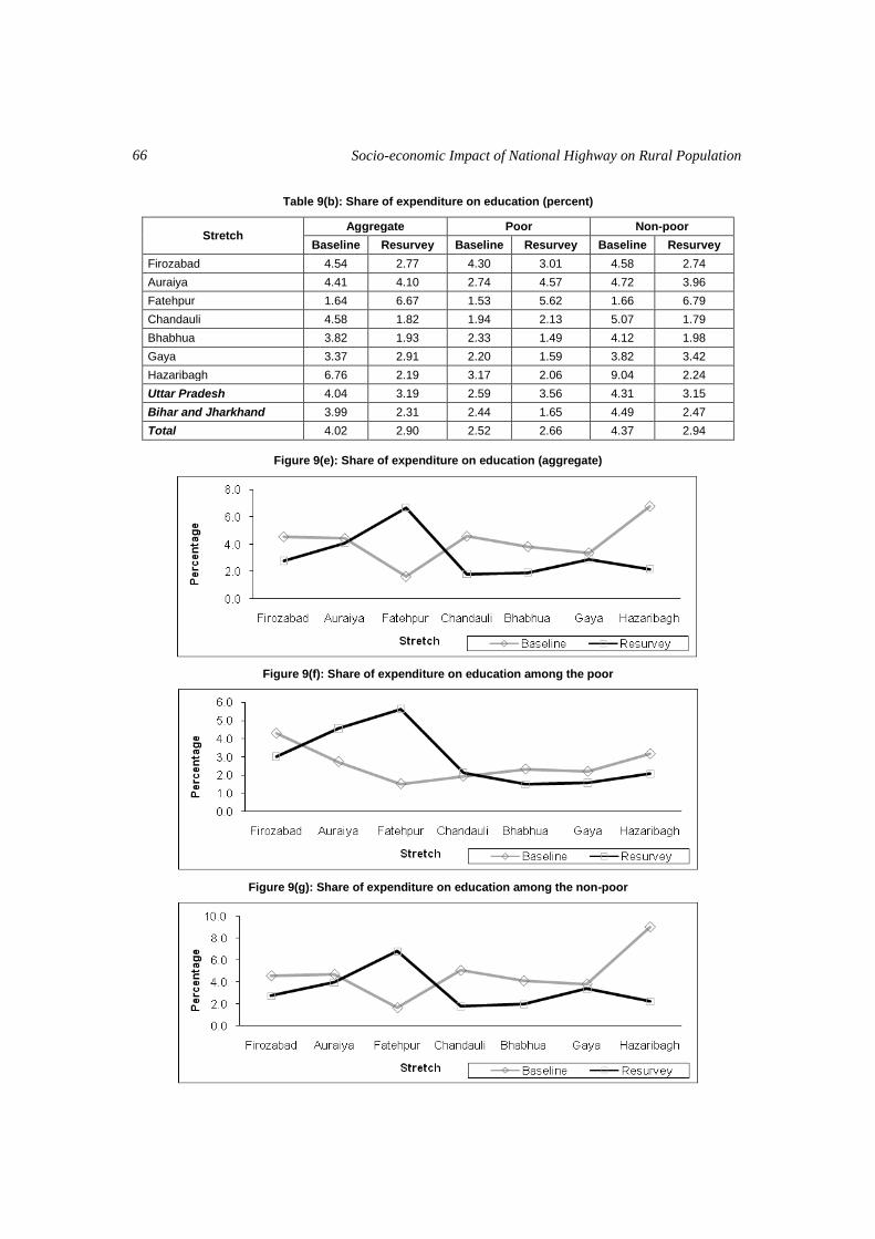
Socio-economic Impact of National Highway on Rural Population 66
Table 9(b): Share of expenditure on education (percent)
Stretch Aggregate Poor Non-poor
Baseline Resurvey Baseline Resurvey Baseline Resurvey
Firozabad 4.54 2.77 4.30 3.01 4.58 2.74
Auraiya 4.41 4.10 2.74 4.57 4.72 3.96
Fatehpur 1.64 6.67 1.53 5.62 1.66 6.79
Chandauli 4.58 1.82 1.94 2.13 5.07 1.79
Bhabhua 3.82 1.93 2.33 1.49 4.12 1.98
Gaya 3.37 2.91 2.20 1.59 3.82 3.42
Hazaribagh 6.76 2.19 3.17 2.06 9.04 2.24
Uttar Pradesh 4.04 3.19 2.59 3.56 4.31 3.15
Bihar and Jharkhand 3.99 2.31 2.44 1.65 4.49 2.47
Total 4.02 2.90 2.52 2.66 4.37 2.94
Figure 9(e): Share of expenditure on education (aggregate)
Figure 9(f): Share of expenditure on education among the poor
Figure 9(g): Share of expenditure on education among the non-poor
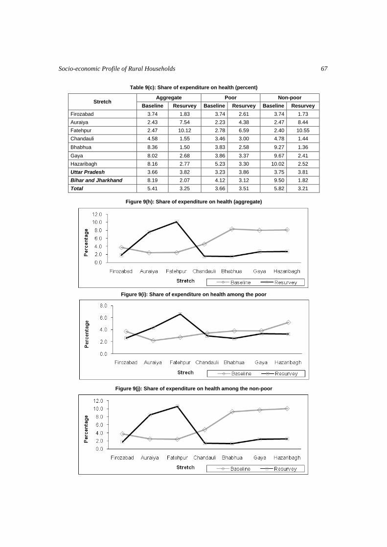
Socio-economic Profile of Rural Households 67
Table 9(c): Share of expenditure on health (percent)
Stretch Aggregate Poor Non-poor
Baseline Resurvey Baseline Resurvey Baseline Resurvey
Firozabad 3.74 1.83 3.74 2.61 3.74 1.73
Auraiya 2.43 7.54 2.23 4.38 2.47 8.44
Fatehpur 2.47 10.12 2.78 6.59 2.40 10.55
Chandauli 4.58 1.55 3.46 3.00 4.78 1.44
Bhabhua 8.36 1.50 3.83 2.58 9.27 1.36
Gaya 8.02 2.68 3.86 3.37 9.67 2.41
Hazaribagh 8.16 2.77 5.23 3.30 10.02 2.52
Uttar Pradesh 3.66 3.82 3.23 3.86 3.75 3.81
Bihar and Jharkhand 8.19 2.07 4.12 3.12 9.50 1.82
Total 5.41 3.25 3.66 3.51 5.82 3.21
Figure 9(h): Share of expenditure on health (aggregate)
Figure 9(i): Share of expenditure on health among the poor
Figure 9(j): Share of expenditure on health among the non-poor

Socio-economic Impact of National Highway on Rural Population 68
Per capita weekly trip rate
Mobility is a direct function of economic activities. Greater mobility enables
people to access better facilities in terms of education, health and market and widens
their job opportunities. As the economy has grown, the aggregate weekly per capita
trip rate (PCTR) has also shown increase in all the stretches, particularly in the state
of Bihar. Furthermore, both the poor and non-poor have benefitted from this
development. Despite this, poor households continue to have lower mobility levels as
compared to the non-poor households. It may be mentioned here that though the per
capita trip rate is higher for Uttar Pradesh compared to Bihar and Jharkhand, the rate
of growth is significantly higher in Bihar and Jharkhand.
Table 10(a): Travel characteristics – Per capita weekly trip rate
Stretch Aggregate Poor Non-poor
Baseline Resurvey Baseline Resurvey Baseline Resurvey
Firozabad 1.02 1.30 0.79 1.09 1.15 1.41
Auraiya 1.04 1.12 0.89 0.85 1.11 1.43
Fatehpur 0.89 1.19 0.76 1.02 0.97 1.29
Chandauli 1.07 1.46 0.95 1.25 1.16 1.56
Bhabhua 0.75 1.21 0.65 1.01 0.85 1.32
Gaya 0.49 1.18 0.39 1.04 0.66 1.32
Hazaribagh 0.80 1.11 0.64 0.93 1.15 1.31
Uttar Pradesh 1.02 1.31 0.86 1.07 1.11 1.45
Bihar and Jharkhand 0.64 1.18 0.52 1.01 0.80 1.32
Total 0.86 1.25 0.68 1.04 1.01 1.40
Figure 10(a): Per capita weekly trip rate (aggregate)
Figure 10(b): Per capita weekly trip rate among the poor

Socio-economic Profile of Rural Households 69
Figure 10(c): Per capita weekly trip rate among the non-poor
Per capita weekly trip length
Improvement in access and availability of transportation services determines
the length of a trip undertaken by an individual. Spatial extension, in turn, leads to
improvement in the availability of economic opportunities. The average per capita
weekly trip length has increased across all the stretches both for the poor and non-
poor households. It is observed that though per capita trip length is higher among the
non-poor compared to the poor in Bihar and Jharkhand, the growth rate registered has
been higher for the poor.
Table 10(b): Travel characteristics – Per capita weekly trip length (km)
Stretch Aggregate Poor Non-poor
Baseline Resurvey Baseline Resurvey Baseline Resurvey
Firozabad 8.97 18.45 8.54 12.52 9.20 21.43
Auraiya 6.07 14.63 4.89 9.29 6.68 20.58
Fatehpur 6.45 14.57 4.81 9.71 7.43 17.35
Chandauli 9.54 17.16 6.75 10.22 11.35 20.24
Bhabhua 6.49 12.43 4.59 7.11 8.35 15.67
Gaya 3.90 10.32 2.59 9.96 5.96 10.68
Hazaribagh 7.41 11.64 3.61 7.56 15.38 16.00
Uttar Pradesh 8.27 16.64 6.59 10.52 9.25 20.10
Bihar and Jharkhand 5.43 11.30 3.40 8.66 8.23 13.53
Total 7.09 14.39 4.91 9.62 8.92 17.58
Figure 10(d): Per capita weekly trip length (aggregate)
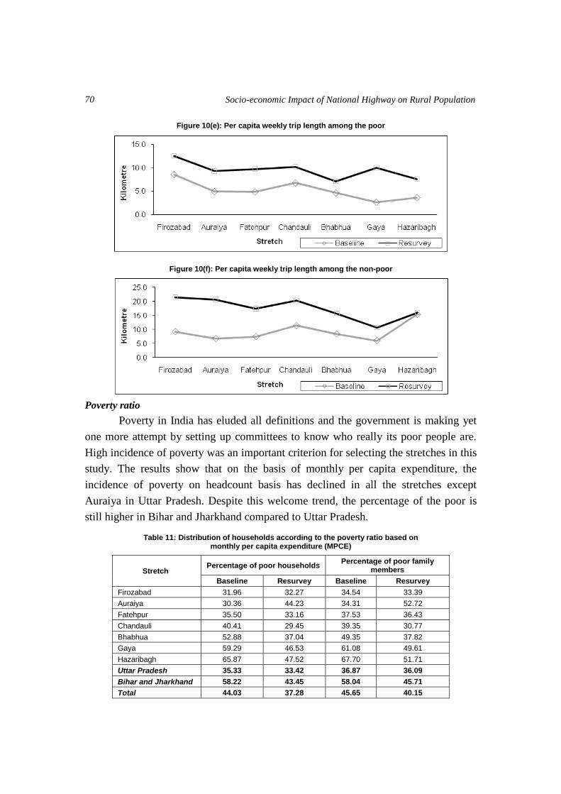
Socio-economic Impact of National Highway on Rural Population 70
Figure 10(e): Per capita weekly trip length among the poor
Figure 10(f): Per capita weekly trip length among the non-poor
Poverty ratio
Poverty in India has eluded all definitions and the government is making yet
one more attempt by setting up committees to know who really its poor people are.
High incidence of poverty was an important criterion for selecting the stretches in this
study. The results show that on the basis of monthly per capita expenditure, the
incidence of poverty on headcount basis has declined in all the stretches except
Auraiya in Uttar Pradesh. Despite this welcome trend, the percentage of the poor is
still higher in Bihar and Jharkhand compared to Uttar Pradesh.
Table 11: Distribution of households according to the poverty ratio based on monthly per capita expenditure (MPCE)
Stretch Percentage of poor households
Percentage of poor family members
Baseline Resurvey Baseline Resurvey
Firozabad 31.96 32.27 34.54 33.39
Auraiya 30.36 44.23 34.31 52.72
Fatehpur 35.50 33.16 37.53 36.43
Chandauli 40.41 29.45 39.35 30.77
Bhabhua 52.88 37.04 49.35 37.82
Gaya 59.29 46.53 61.08 49.61
Hazaribagh 65.87 47.52 67.70 51.71
Uttar Pradesh 35.33 33.42 36.87 36.09
Bihar and Jharkhand 58.22 43.45 58.04 45.71
Total 44.03 37.28 45.65 40.15
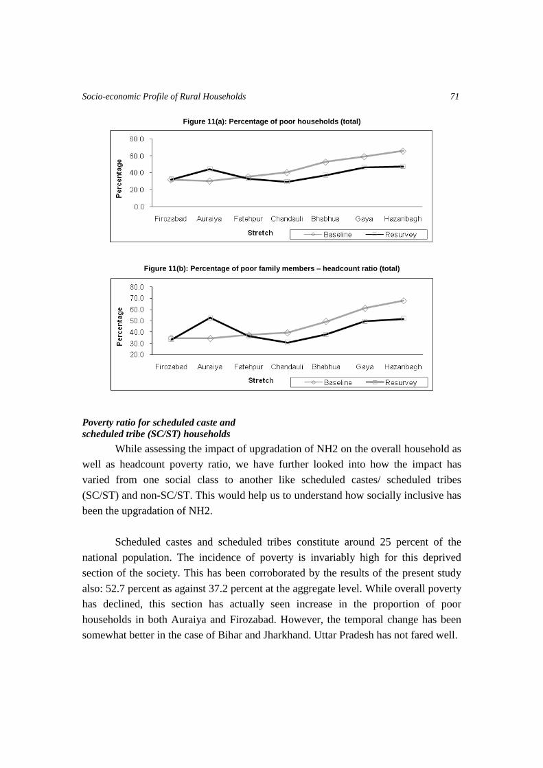
Socio-economic Profile of Rural Households 71
Figure 11(a): Percentage of poor households (total)
Figure 11(b): Percentage of poor family members – headcount ratio (total)
Poverty ratio for scheduled caste and
scheduled tribe (SC/ST) households
While assessing the impact of upgradation of NH2 on the overall household as
well as headcount poverty ratio, we have further looked into how the impact has
varied from one social class to another like scheduled castes/ scheduled tribes
(SC/ST) and non-SC/ST. This would help us to understand how socially inclusive has
been the upgradation of NH2.
Scheduled castes and scheduled tribes constitute around 25 percent of the
national population. The incidence of poverty is invariably high for this deprived
section of the society. This has been corroborated by the results of the present study
also: 52.7 percent as against 37.2 percent at the aggregate level. While overall poverty
has declined, this section has actually seen increase in the proportion of poor
households in both Auraiya and Firozabad. However, the temporal change has been
somewhat better in the case of Bihar and Jharkhand. Uttar Pradesh has not fared well.
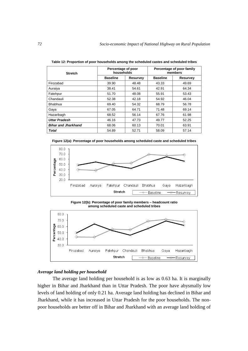
Socio-economic Impact of National Highway on Rural Population 72
Table 12: Proportion of poor households among the scheduled castes and scheduled tribes
Stretch
Percentage of poor households
Percentage of poor family members
Baseline Resurvey Baseline Resurvey
Firozabad 39.90 48.48 43.33 49.69
Auraiya 38.41 54.61 42.91 64.34
Fatehpur 51.70 48.08 55.91 53.43
Chandauli 52.38 42.18 54.92 46.04
Bhabhua 69.40 54.32 68.79 56.78
Gaya 67.05 64.71 71.48 69.14
Hazaribagh 68.52 56.14 67.76 61.98
Uttar Pradesh 46.16 47.73 49.77 52.25
Bihar and Jharkhand 68.06 60.13 70.01 63.91
Total 54.89 52.71 58.09 57.14
Figure 12(a): Percentage of poor households among scheduled caste and scheduled tribes
Figure 12(b): Percentage of poor family members – headcount ratio among scheduled caste and scheduled tribes
Average land holding per household
The average land holding per household is as low as 0.63 ha. It is marginally
higher in Bihar and Jharkhand than in Uttar Pradesh. The poor have abysmally low
levels of land holding of only 0.21 ha. Average land holding has declined in Bihar and
Jharkhand, while it has increased in Uttar Pradesh for the poor households. The non-
poor households are better off in Bihar and Jharkhand with an average land holding of
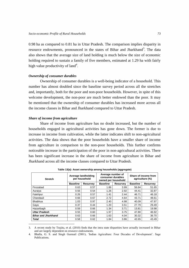
Socio-economic Profile of Rural Households 73
0.98 ha as compared to 0.81 ha in Uttar Pradesh. The comparison implies disparity in
resource endowments, pronounced in the states of Bihar and Jharkhand3. The data
also shows that the average size of land holding is much below the size of economic
holding required to sustain a family of five members, estimated at 1.29 ha with fairly
high value productivity of land4.
Ownership of consumer durables
Ownership of consumer durables is a well-being indicator of a household. This
number has almost doubled since the baseline survey period across all the stretches
and, importantly, both for the poor and non-poor households. However, in spite of this
welcome development, the non-poor are much better endowed than the poor. It may
be mentioned that the ownership of consumer durables has increased more across all
the income classes in Bihar and Jharkhand compared to Uttar Pradesh.
Share of income from agriculture
Share of income from agriculture has no doubt increased, but the number of
households engaged in agricultural activities has gone down. The former is due to
increase in income from cultivation, while the latter indicates shift to non-agricultural
activities. The data shows that the poor households have a smaller share of income
from agriculture in comparison to the non-poor households. This further confirms
noticeable increase in the participation of the poor in non-agricultural activities. There
has been significant increase in the share of income from agriculture in Bihar and
Jharkhand across all the income classes compared to Uttar Pradesh.
Table 13(a): Asset ownership among households (aggregate)
Stretch
Average landholding per household
Average number of consumer durables
owned per household
Share of income from agriculture (%)
Baseline Resurvey Baseline Resurvey Baseline Resurvey
Firozabad 0.63 0.57 1.86 3.99 56.84 51.65
Auraiya 0.56 0.54 1.26 2.92 44.41 32.87
Fatehpur 0.26 0.57 1.41 2.44 46.71 46.18
Chandauli 0.66 0.67 2.72 4.64 43.71 48.61
Bhabhua 1.03 0.97 2.40 4.98 40.09 47.97
Gaya 0.37 0.44 1.20 3.51 27.79 29.49
Hazaribagh 0.59 0.66 1.34 3.71 13.81 19.98
Uttar Pradesh 0.55 0.60 1.97 3.75 47.80 46.92
Bihar and Jharkhand 0.63 0.66 1.63 4.04 30.32 36.70
Total 0.58 0.62 1.84 3.86 42.65 43.49
3. A recent study by Tsujita, et al. (2010) finds that the intra state disparities have actually increased in Bihar
and are largely dependent on resource endowments.
4. Bhalla, G. S. and Singh Gurmail (2001), ‘Indian Agriculture: Four Decades of Development’. Sage
Publications.
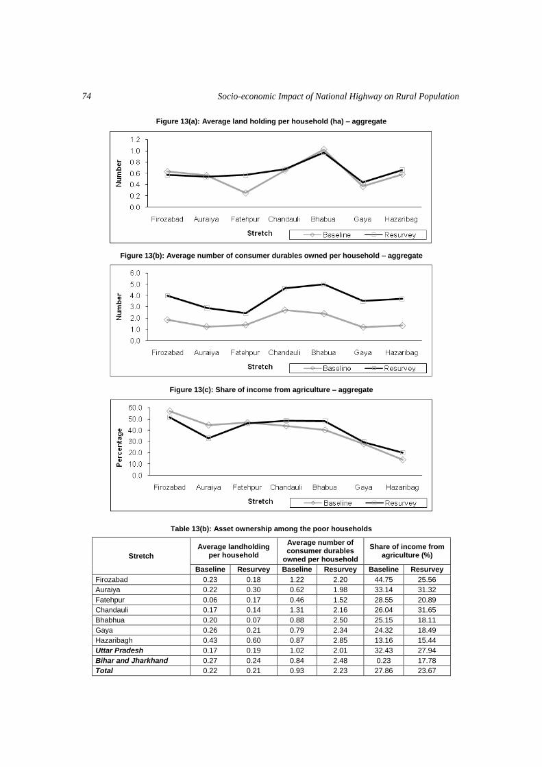
Socio-economic Impact of National Highway on Rural Population 74
Figure 13(a): Average land holding per household (ha) – aggregate
Figure 13(b): Average number of consumer durables owned per household – aggregate
Figure 13(c): Share of income from agriculture – aggregate
Table 13(b): Asset ownership among the poor households
Stretch
Average landholding per household
Average number of consumer durables
owned per household
Share of income from agriculture (%)
Baseline Resurvey Baseline Resurvey Baseline Resurvey
Firozabad 0.23 0.18 1.22 2.20 44.75 25.56
Auraiya 0.22 0.30 0.62 1.98 33.14 31.32
Fatehpur 0.06 0.17 0.46 1.52 28.55 20.89
Chandauli 0.17 0.14 1.31 2.16 26.04 31.65
Bhabhua 0.20 0.07 0.88 2.50 25.15 18.11
Gaya 0.26 0.21 0.79 2.34 24.32 18.49
Hazaribagh 0.43 0.60 0.87 2.85 13.16 15.44
Uttar Pradesh 0.17 0.19 1.02 2.01 32.43 27.94
Bihar and Jharkhand 0.27 0.24 0.84 2.48 0.23 17.78
Total 0.22 0.21 0.93 2.23 27.86 23.67

Socio-economic Profile of Rural Households 75
Figure 13(d): Average land holding per household (ha) among the poor
Figure 13(e): Average number of consumer durables owned per household among the poor
Figure 13(f): Share of income from agriculture among the poor
Table 13(c): Asset ownership among the non-poor households
Stretch
Average landholding per household
Av no of consumer durables owned per
household
Share of income from agriculture (%)
Baseline Resurvey Baseline Resurvey Baseline Resurvey
Firozabad 0.63 0.76 1.86 4.80 56.84 57.12
Auraiya 0.56 0.74 1.26 3.63 44.41 33.62
Fatehpur 0.26 0.78 1.41 2.88 46.71 50.71
Chandauli 0.66 0.88 2.72 5.66 43.71 51.17
Bhabhua 1.03 1.5 2.40 6.44 40.09 53.79
Gaya 0.37 0.63 1.20 4.54 27.79 34.37
Hazaribagh 0.59 0.71 1.34 4.51 13.81 22.45
Uttar Pradesh 0.55 0.81 1.97 4.58 47.80 50.86
Bihar and Jharkhand 0.63 0.98 1.63 5.25 0.32 42.91
Total 0.58 0.87 1.84 4.81 42.65 48.35
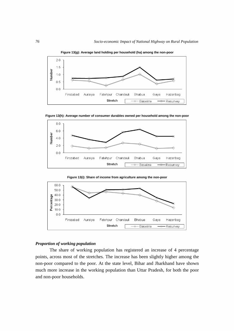
Socio-economic Impact of National Highway on Rural Population 76
Figure 13(g): Average land holding per household (ha) among the non-poor
Figure 13(h): Average number of consumer durables owned per household among the non-poor
Share of income from agriculture – non-poor
Figure 13(i): Share of income from agriculture among the non-poor
Proportion of working population
The share of working population has registered an increase of 4 percentage
points, across most of the stretches. The increase has been slightly higher among the
non-poor compared to the poor. At the state level, Bihar and Jharkhand have shown
much more increase in the working population than Uttar Pradesh, for both the poor
and non-poor households.

Socio-economic Profile of Rural Households 77
Table 14: Proportion of working population (percent)
Stretch Aggregate Poor Non-poor
Baseline Resurvey Baseline Resurvey Baseline Resurvey
Firozabad 28.00 32.54 25.06 30.53 29.55 33.55
Auraiya 30.68 33.61 27.44 31.00 32.37 36.51
Fatehpur 31.39 36.26 29.45 34.37 32.56 37.34
Chandauli 29.10 33.54 29.75 31.64 28.68 34.39
Bhabhua 26.90 32.42 26.88 33.31 26.92 31.89
Gaya 29.96 36.65 29.32 35.94 30.98 37.35
Hazaribagh 28.71 31.27 28.34 28.61 29.49 34.12
Uttar Pradesh 29.45 33.77 28.11 31.71 30.24 34.94
Bihar and Jharkhand 28.66 34.23 28.39 33.77 29.03 34.62
Total 29.12 33.97 28.26 32.70 29.85 34.81
Figure 14(a): Proportion of working population (aggregate)
Proportion of working population among poor
Figure 14(b): Proportion of working population among the poor
Figure 14(c): Proportion of working population among the non-poor

Socio-economic Impact of National Highway on Rural Population 78
Proportion of working population among females
The participation of women in the workforce contributes to both social
awareness and well-being. In the present study, the proportion of working women in
the total female population has registered manifold increase, across all selected
stretches and economic classes, with Bihar and Jharkhand registering more increase
compared to Uttar Pradesh. Generally, the female workforce participation rates are
higher in the poor households and this was the position at the time of the baseline
survey. In the interregnum, this has undergone a dramatic change: the percentage rates
of working women both for the poor and non-poor households have leveled off.
Table 15: Proportion of working women in the female population (percent)
Stretch Aggregate Poor Non-poor
Baseline Resurvey Baseline Resurvey Baseline Resurvey
Firozabad 2.47 8.93 1.69 7.25 2.90 9.78
Auraiya 3.14 11.04 1.77 9.76 3.84 12.44
Fatehpur 6.30 15.57 8.15 14.81 5.11 16.01
Chandauli 7.47 14.55 10.36 13.83 5.56 14.87
Bhabhua 3.49 14.40 4.36 18.35 2.63 11.99
Gaya 6.85 20.36 7.47 19.19 5.88 21.57
Hazaribagh 5.02 8.72 4.53 6.84 6.01 10.88
Uttar Pradesh 5.21 12.61 6.48 11.38 4.44 13.31
Bihar and Jharkhand 5.33 16.25 5.93 16.57 4.51 15.97
Total 5.26 14.18 6.19 13.94 4.46 14.35
Figure 15(a): Proportion of working women in the female population (aggregate)
Figure 15(b): Proportion of working women in the female population among the poor
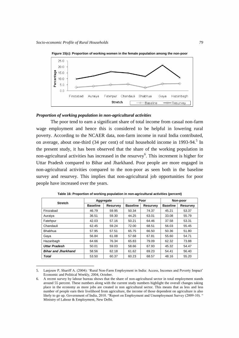
Socio-economic Profile of Rural Households 79
Figure 15(c): Proportion of working women in the female population among the non-poor
Proportion of working population in non-agricultural activities
The poor tend to earn a significant share of total income from casual non-farm
wage employment and hence this is considered to be helpful in lowering rural
poverty. According to the NCAER data, non-farm income in rural India contributed,
on average, about one-third (34 per cent) of total household income in 1993-94.5 In
the present study, it has been observed that the share of the working population in
non-agricultural activities has increased in the resurvey6. This increment is higher for
Uttar Pradesh compared to Bihar and Jharkhand. Poor people are more engaged in
non-agricultural activities compared to the non-poor as seen both in the baseline
survey and resurvey. This implies that non-agricultural job opportunities for poor
people have increased over the years.
Table 16: Proportion of working population in non-agricultural activities (percent)
Stretch Aggregate Poor Non-poor
Baseline Resurvey Baseline Resurvey Baseline Resurvey
Firozabad 46.79 59.95 50.34 74.37 45.21 53.37
Auraiya 36.51 59.30 44.25 63.01 33.08 55.79
Fatehpur 42.03 57.16 50.21 64.46 37.58 53.31
Chandauli 62.45 59.24 72.00 68.51 56.03 55.45
Bhabhua 57.95 57.51 65.75 66.50 50.36 51.80
Gaya 56.84 61.08 57.68 67.81 55.60 54.71
Hazaribagh 64.66 76.34 65.83 79.09 62.32 73.88
Uttar Pradesh 50.01 59.03 58.66 67.93 45.32 54.47
Bihar and Jharkhand 58.56 62.18 61.62 69.23 54.41 56.40
Total 53.50 60.37 60.23 68.57 48.16 55.20
5. Lanjouw P, Shariff A. (2004): ‘Rural Non-Farm Employment in India: Access, Incomes and Poverty Impact’
Economic and Political Weekly, 2004, October.
6. A recent survey by labour bureau shows that the share of non-agricultural sector in total employment stands
around 55 percent. These numbers along with the current study numbers highlight the overall changes taking
place in the economy as more jobs are created in non agricultural sector. This means that as less and less
number of people earn their livelihood from agriculture, the income of those dependent on agriculture is also
likely to go up. Government of India, 2010. “Report on Employment and Unemployment Survey (2009-10). “
Ministry of Labour & Employment, New Delhi.
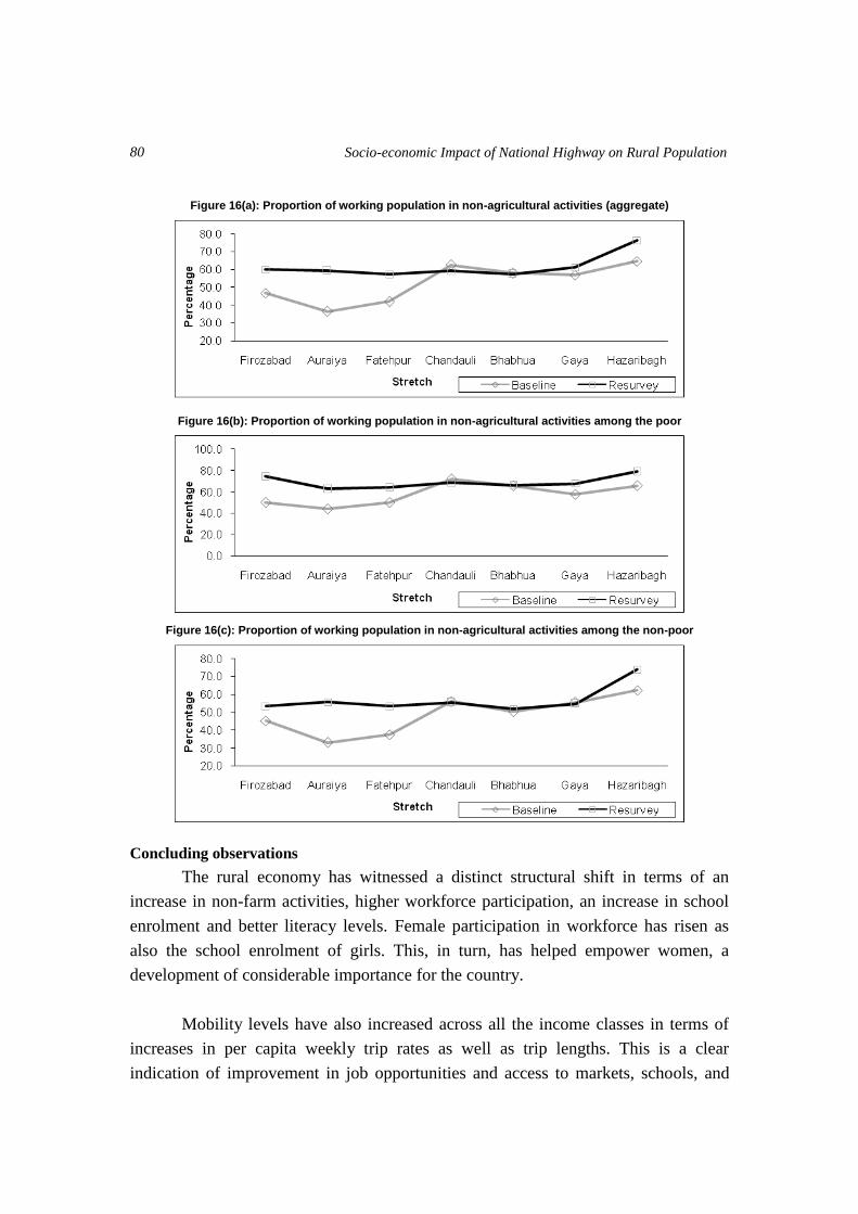
Socio-economic Impact of National Highway on Rural Population 80
Figure 16(a): Proportion of working population in non-agricultural activities (aggregate)
Figure 16(b): Proportion of working population in non-agricultural activities among the poor
Figure 16(c): Proportion of working population in non-agricultural activities among the non-poor
Concluding observations
The rural economy has witnessed a distinct structural shift in terms of an
increase in non-farm activities, higher workforce participation, an increase in school
enrolment and better literacy levels. Female participation in workforce has risen as
also the school enrolment of girls. This, in turn, has helped empower women, a
development of considerable importance for the country.
Mobility levels have also increased across all the income classes in terms of
increases in per capita weekly trip rates as well as trip lengths. This is a clear
indication of improvement in job opportunities and access to markets, schools, and

Socio-economic Profile of Rural Households 81
other services. This is also a sign of increase in the spatial distribution of economic
activities.
Economic growth and development have been widespread and largely
inclusive. However, the effects of such development have not been uniform across
time or across economic classes. Although the differences have remained they have
substantially narrowed. With Bihar and Jharkhand showing greater improvement, the
disparities have considerably reduced.
The non-poor or not-so-poor have benefitted more than the poorer ones. This
is perhaps typical of the early days of development as better-off persons have better
access to facilities. As time goes by, it can be expected that benefits would become
more even.
Human dignity depends to a great extent on education. Labour productivity in
the long run is also a function of the levels of schooling received. Average school
enrolment among children has increased to more than 90 percent. Significantly, the
enrolment level among the poor households has also been high – 86 percent.
Furthermore, Bihar and Jharkhand have shown considerable improvement in this
regard. All these developments have long-term beneficial implications.
The overall literacy level has improved across all the stretches, but it is still
somewhat lower than the national average. The interstate and class differences also
persist. For example, for the poor households, literacy is 17 percent less compared to
the non-poor households. However, the female literacy rate among the poor
households has increased at a much faster rate than the non-poor households.
It is now well-established that the individual and social returns from the
women’s education are exceptionally high, especially in the matter of lowering of
fertility and infant and child mortality rates, and improvement in the children’s
educational achievements. There has been a significant rise in school enrolment
among girls even in the poor households. In this respect, both Bihar and Jharkhand
have done well.
The proportion of working women in the total female population has
registered a manifold increase across all economic classes, with Bihar and Jharkhand

Socio-economic Impact of National Highway on Rural Population 82
registering higher increase. Generally, the female workforce participation rates are
higher in the poor households. This position has undergone a dramatic change. The
women from not-so-poor households are also equally participating in the workforce.
The overall sex ratio (number of females per 1000 males) has remained
unchanged and continues to be lower than the national average. The poor households
have a higher sex ratio than the non-poor households. Arguably, better-off
communities have a stronger gender bias against the female than poor households.
In terms of poverty indicators, the proportion of people living below the
poverty line has declined significantly for all the stretches except Auraiya in Uttar
Pradesh both on an overall basis and headcount basis. For scheduled castes and
scheduled tribes, this proportion has also reduced for all the stretches except at two
places in Uttar Pradesh, viz., Auraiya and Firozabad, both on an overall basis and
headcount basis.
The average landholding per household is low at 0.63 hectare, with marginally
higher holdings in Bihar and Jharkhand. There is pronounced disparity in resource
endowments across the economic classes. The average landholding of a poor
household is abysmally low – one-eighth of a hectare in Uttar Pradesh and a quarter
of a hectare in Bihar and Jharkhand. The non-poor households are better off,
particularly in Bihar and Jharkhand with an average landholding of 0.98 hectare.
The share of income from agriculture particularly in Bihar and Jharkhand has
increased but the number of households engaged in agricultural activities has gone
down in all the representative stretches. The poor households have a smaller share of
income from agriculture in comparison to the non-poor households. However, in case
of poor households, their share from non-agricultural activities has increased.
Chapter 4
Impact Evaluation at Village Level
As mentioned elsewhere in the report, the socio-economic impact analysis of a
public investment project (like the present one of 4-laning of NH2) is made to
determine the extent of the net socio-economic benefits of the project that accrue to
the population group(s) concerned, with a focus on poverty alleviation. Typically,
such analysis comprises two studies of the socio-economic conditions of these
group(s) – one, based on baseline survey data (collected before the project is
launched) and the other, based on the resurvey data (collected after the project has
been completed). The partial effects of the project are then assessed by appropriately
comparing and interpreting the results of these two studies. This report presents the
results of a study of the impact analysis of widening of the NH2 based on the
comparison of the socio-economic conditions of the population living around the
stretch of NH2 being widened, before and after the project.
The rationale of the present study is based on the premise that, ceteris paribus,
access to a highway provides to the population living in its appropriately defined
neighbourhood opportunities that help improve their well-being. To verify this
presumption empirically, the relationship between the selected village-level indicators
of socio-economic well-being and the proximity of villages to NH2 has been
examined. This relationship is further influenced by the quality and width of the
highway and is therefore indicative of the positive impact of highway widening.
Three different statistical/econometric techniques, viz., correlation analysis, non-
parametric regression analysis, and comparison of means have been used to analyse
the baseline and the resurvey data collected. The results of these analyses are
presented in the following sections.
Village level variables
For the present analysis, 16 village-level socio-economic variables that are
likely to be influenced directly or indirectly by the proximity of the villages to NH2
have been considered (Table 1). These variables may be categorised into seven
groups. Of these, five groups, viz., incidence of poverty, transport infrastructure,
employment, asset ownership, and education and other infrastructure, relate to the
well-being of the population. Another group relates to the demographic characteristics
which reflect the role of better economic opportunities arising from proximity to
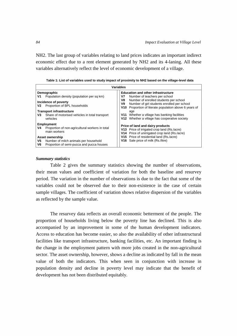
84 Impact Evaluation at Village Level
NH2. The last group of variables relating to land prices indicates an important indirect
economic effect due to a rent element generated by NH2 and its 4-laning. All these
variables alternatively reflect the level of economic development of a village.
Table 1: List of variables used to study impact of proximity to NH2 based on the village-level data
Variables
Demographic V1 Population density (population per sq km)
Education and other infrastructure V7 Number of teachers per school V8 Number of enrolled students per school V9 Number of girl students enrolled per school V10 Proportion of literate population above 6 years of
age V11 Whether a village has banking facilities V12 Whether a village has cooperative society Price of land and dairy products V13 Price of irrigated crop land (Rs./acre) V14 Price of unirrigated crop land (Rs./acre) V15 Price of residential land (Rs./acre) V16 Sale price of milk (Rs./litre)
Incidence of poverty V2 Proportion of BPL households
Transport infrastructure V3 Share of motorised vehicles in total transport
vehicles
Employment V4 Proportion of non-agricultural workers in total
main workers
Asset ownership V5 Number of milch animals per household V6 Proportion of semi-pucca and pucca houses
Summary statistics
Table 2 gives the summary statistics showing the number of observations,
their mean values and coefficient of variation for both the baseline and resurvey
period. The variation in the number of observations is due to the fact that some of the
variables could not be observed due to their non-existence in the case of certain
sample villages. The coefficient of variation shows relative dispersion of the variables
as reflected by the sample value.
The resurvey data reflects an overall economic betterment of the people. The
proportion of households living below the poverty line has declined. This is also
accompanied by an improvement in some of the human development indicators.
Access to education has become easier, so also the availability of other infrastructural
facilities like transport infrastructure, banking facilities, etc. An important finding is
the change in the employment pattern with more jobs created in the non-agricultural
sector. The asset ownership, however, shows a decline as indicated by fall in the mean
value of both the indicators. This when seen in conjunction with increase in
population density and decline in poverty level may indicate that the benefit of
development has not been distributed equitably.

85 Impact Evaluation at Village Level
Table 2: Summary of selected demographic and socio-economic impact indicators at village level
Variable
Baseline Resurvey
Number of obser-vations
Mean value Coefficient of variation
(percent)
Number of obser-vations
Mean value Coefficient of variation
(percent)
V0 Approach distance from NH2 (in km) 200 4.34 79.26 200 4.34 79.26
Demographic
V1 Population density 200 564.34 59.72 200 723.13 132.45
Incidence of poverty
V2 Proportion of BPL households 200 38.23 62.43 200 34.70 85.21
Transport infrastructure
V3 Share of motorised vehicles in total transport vehicles 200 8.56 80.16 200 16.00 76.76
Employment
V4 Proportion of non-agricultural workers in total main workers 200 19.56 127.73 199 35.65 78.16
Asset ownership
V5 Number of milch animals per household 200 1.87 67.98 200 1.12 123.30
V6 Proportion of semi-pucca and pucca houses 200 60.31 60.25 200 54.80 54.19
Education and other infrastructure
V7 Number of teachers per school 151 3.28 60.8 167 4.16 49.86
V8 Number of enrolled students per school 151 55.43 118.3 167 133.12 70.72
V9 Number of girl students enrolled per school 151 23.14 105.84 167 59.39 73.32
V10 Proportion of literate population above 6 years of age 200 43.27 44.27 200 59.35 28.76
V11 Whether a village has banking facilities 200 12 36.83 200 138.00 67.20
V12 Whether a village has cooperative society 200 19.5 203.69 200 83.00 119.03
Price of land and dairy products
V13 Price of irrigated crop land (Rs./acre) 200.00 186,243.75 63.09 200 826,105.56 194.42
V14 Price of unirrigated crop land (Rs./acre) 187.00 117,940.00 85.58 186 191,494.74 79.95
V15 Price of residential land (Rs./acre) 200.00 427,005.00 114.99 200 2,734,254.64 377.66
V16 Sale price of milk (Rs./litre) 200.00 10.46 22.47 200 13.87 16.83
Note: The demographic data is based on Census of India, 1991, 2001 has been extrapolated for the relevant survey years
Correlation analysis
For a preliminary analysis, the pattern of interdependence among various
chosen variables has been examined using the simple correlation coefficient between
pairs of variables. As is well known, the correlation coefficient is an index of the
degree of linear dependence of a pair of variables as present in a given data set. The
computed correlation matrix is presented in Table 3.
Table 3: Correlation among selected socio-economic indicators at village level
V0 V1 V2 V3 V4 V5 V6 V7 V8 V9 V10 V11 V12 V13 V14 V15 V16
V0 1
V1 -0.1787* 1
V2 -0.119 -0.1316 1
V3 -0.0667 0.0335 0.0051 1
V4 -0.2235* 0.2041 0.0219 0.0386 1
V5 0.0856 -0.1953 0.1352 0.144 -0.0494 1
V6 -0.1724* 0.0772 -0.2245 0.148 0.2057 0.0156 1
V7 -0.1127 0.1525 0.0424 0.0808 0.1479 -0.0033 0.0841 1
V8 -0.0711 0.0788 0.0858 0.0431 0.0584 0.0002 -0.3432 0.2245 1
V9 -0.0537 0.0674 0.0278 0.056 0.0323 -0.0544 -0.3092 0.1961 0.9497 1
V10 0.0412 -0.0526 -0.1826 0.1183 0.298 0.0133 0.5512 0.1415 -0.1708 -0.1428 1
V11 0.0368 0.0136 -0.0364 0.0642 0.0562 0.109 0.1936 0.0676 0.0492 0.0382 0.1707 1
V12 0.0011 -0.0205 0.0949 -0.1353 -0.0257 -0.0824 -0.2121 0.1234 0.2271 0.2357 -0.249 -0.1595 1
V13 -0.0827 0.1211 0.121 -0.0103 0.2355 -0.0514 -0.1005 0.0617 0.1843 0.1778 -0.0017 0.1159 -0.0317 1
V14 0.0351 0.2018 0.0502 0.0284 0.1254 -0.1092 -0.0406 0.2289 0.2189 0.1925 -0.001 -0.0331 0.0789 0.1201 1
V15 -0.1328 0.0506 0.0142 -0.0453 0.1941 -0.0541 -0.0791 0.0829 0.1162 0.0927 -0.082 0.0369 0.1164 0.1114 0.2179 1
V16 0.1057 -0.065 0.0657 0.0104 -0.2038 0.0649 -0.2925 0.0881 0.2747 0.2717 -0.2733 -0.062 0.1641 -0.0158 0.0233 -0.0222 1
Note: * are significant at 5 percent level with the distance from NH2 V0: denotes approach distance of the village from NH2 (km)

86 Impact Evaluation at Village Level
As the above results suggest, the degree of pair-wise association with V0 (i.e.
distance from NH2) is significant with the expected sign for three of the chosen well-
being indicator variables – population density (V1), proportion of non-agricultural
workers in total main workers (V4) and proportion of semi-pucca and pucca houses
(V6). Importantly, these three correlations were also found to be statistically
significant in the baseline analysis.
Table 3 also provides information on the degree of correlation between pairs
of chosen ‘well-being’ indicators. It may be noted that, except in a few cases, such
correlation is not strong. This suggests that, by and large, the chosen ‘well-being’
indicators reflect diverse aspects of well-being which are not closely related to one
another.
The cases of strong correlation include the association between the proportion
of semi-pucca and pucca houses and proportion of literate population above 6 years of
age and between the number of enrolled students per school and the number of girl
students enrolled per school. Significantly, these pairs of variables had also shown
strong correlation in the baseline analysis. Importantly, this relationship has become
stronger in the resurvey.
In sum, the correlation matrix suggests that there are higher job opportunities
available for non-agricultural workers in closer proximity of the highway. This
attribute also influences demographic characteristics in terms of density of population
in nearby habitations. Better housing conditions are indicative of their economic well-
being.
Comparison of means analysis
As a preliminary analysis, it has been examined whether the mean values of a
variable for the influence and control zones are equal. This has been done by testing
for each variable the null hypothesis that population means for two zones are the
same1. The comparison of overall means for the two zones provides a benchmark of
measurement of the differences in the average levels of various impact variables
between the influence and control zones. Table 4 presents the mean values of the 16
selected village-level indicators of well-being for the two groups of villages in the
influence and control zones. The table also provides the single difference between the
1. The significance of means has been tested using t-statistics.
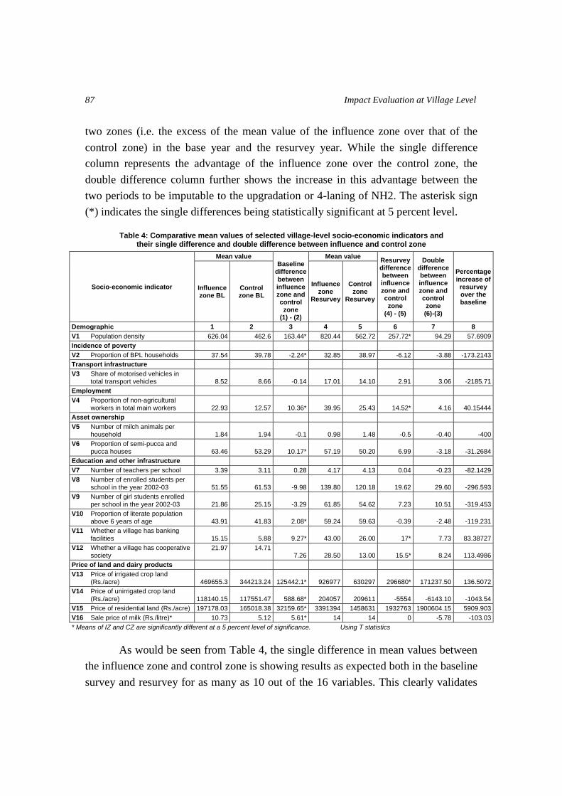
87 Impact Evaluation at Village Level
two zones (i.e. the excess of the mean value of the influence zone over that of the
control zone) in the base year and the resurvey year. While the single difference
column represents the advantage of the influence zone over the control zone, the
double difference column further shows the increase in this advantage between the
two periods to be imputable to the upgradation or 4-laning of NH2. The asterisk sign
(*) indicates the single differences being statistically significant at 5 percent level.
Table 4: Comparative mean values of selected village-level socio-economic indicators and
their single difference and double difference between influence and control zone
Socio-economic indicator
Mean value Baseline
difference between influence zone and control zone
(1) - (2)
Mean value Resurvey difference between influence zone and control zone
(4) - (5)
Double difference between influence zone and control zone (6)-(3)
Percentage increase of resurvey over the baseline
Influence zone BL
Control zone BL
Influence zone
Resurvey
Control zone
Resurvey
Demographic 1 2 3 4 5 6 7 8
V1 Population density 626.04 462.6 163.44* 820.44 562.72 257.72* 94.29 57.6909
Incidence of poverty
V2 Proportion of BPL households 37.54 39.78 -2.24* 32.85 38.97 -6.12 -3.88 -173.2143
Transport infrastructure
V3 Share of motorised vehicles in total transport vehicles 8.52 8.66 -0.14 17.01 14.10 2.91 3.06 -2185.71
Employment
V4 Proportion of non-agricultural workers in total main workers 22.93 12.57 10.36* 39.95 25.43 14.52* 4.16 40.15444
Asset ownership
V5 Number of milch animals per
household 1.84 1.94 -0.1 0.98 1.48 -0.5 -0.40 -400
V6 Proportion of semi-pucca and pucca houses 63.46 53.29 10.17* 57.19 50.20 6.99 -3.18 -31.2684
Education and other infrastructure
V7 Number of teachers per school 3.39 3.11 0.28 4.17 4.13 0.04 -0.23 -82.1429
V8 Number of enrolled students per school in the year 2002-03 51.55 61.53 -9.98 139.80 120.18 19.62 29.60 -296.593
V9 Number of girl students enrolled per school in the year 2002-03 21.86 25.15 -3.29 61.85 54.62 7.23 10.51 -319.453
V10 Proportion of literate population above 6 years of age 43.91 41.83 2.08* 59.24 59.63 -0.39 -2.48 -119.231
V11 Whether a village has banking facilities 15.15 5.88 9.27* 43.00 26.00 17* 7.73 83.38727
V12 Whether a village has cooperative society
21.97 14.71 7.26 28.50 13.00 15.5* 8.24 113.4986
Price of land and dairy products
V13 Price of irrigated crop land (Rs./acre) 469655.3 344213.24 125442.1* 926977 630297 296680* 171237.50 136.5072
V14 Price of unirrigated crop land (Rs./acre) 118140.15 117551.47 588.68* 204057 209611 -5554 -6143.10 -1043.54
V15 Price of residential land (Rs./acre) 197178.03 165018.38 32159.65* 3391394 1458631 1932763 1900604.15 5909.903
V16 Sale price of milk (Rs./litre)* 10.73 5.12 5.61* 14 14 0 -5.78 -103.03
* Means of IZ and CZ are significantly different at a 5 percent level of significance. Using T statistics
As would be seen from Table 4, the single difference in mean values between
the influence zone and control zone is showing results as expected both in the baseline
survey and resurvey for as many as 10 out of the 16 variables. This clearly validates
88 Impact Evaluation at Village Level
the ‘basic neighbourhood premise’ for studying the well-being of the population
living in the proximity of the national highway.
In the resurvey, five variables – population density (V1), proportion of non-
agricultural workers in total main workers (V4), availability of banking facilities
(V11) availability of cooperative society (V12) and price of irrigated crop land (V13)
– have shown not only significant differences in mean values but their magnitude has
also increased as compared to the baseline mean values.
Furthermore, irrespective of the significance, the percentage improvement in
single differences of the resurvey over the baseline survey has also turned out to be
positive for 50 percent of the variables, thereby reflecting positive impact of highway
after its upgradation. These relate to population density (V1), proportion of BPL
households (V2), proportion of non-agricultural workers in total main workers (V4),
enrolment of students in schools (V8), enrolment of girl students in schools (V9),
availability of banking facility (V11), availability of cooperative societies (V12) price
of irrigated crop land (V13) and price of residential land (V15).
Non-parametric regression analysis
For a more rigorous examination of the extent and nature of the association of
selected well-being indicators with approach distance of a village from the highway
based on the available village-level data, we have used the bi-variate non-parametric
regression analysis (Chapter 1 explains this econometric technique). To be more
specific, for each of the sixteen well-being indicator variables, the graphs of the
estimated non-parametric regression of the variable concerned on the distance from
the highway have been obtained for both the baseline survey data and the resurvey
data for the entire range of variation of the distance variable for the villages as
covered by the said surveys. This range has been almost 8 km. These graphs are
expected to show the gradient of change with a negative slope of a specific well-being
indicator for which a higher value is better in relation to the distance from the
highway.
The results of the non-parametric regression analysis have brought out the
well-behaved relationship with distance from the highway for most of the well-being
indicator variables implicit in the village-level data set. In each of these cases, the
estimated relationship is observed to be a monotonic one over either the entire range

89 Impact Evaluation at Village Level
of distance or up to a critical distance, which varies from one indicator to another. The
graphs of the estimated non-parametric regression relationships are presented for both
the surveys and explained in the following section.
Demographic implications
As Figure 1 shows, the population density of a village tends to decline
monotonically as the distance from NH2 increases for both the baseline and resurvey
years. Such a pattern suggests that the villages in the vicinity of the highway have a
much better prospect of
having diversified economic
activities which, among
other things, induce a higher
population density. Here, it
may be pointed out that the
level of population density
at all distance levels has
become higher in the
resurvey after the
upgradation of the highway. It is, however, more pronounced up to a distance of
3 km, suggesting that ease of commuting also plays a reinforcing role.
Incidence of poverty
Figure 2 indicates that as per the baseline data, the percentage of households
living below the poverty line (BPL) monotonically increases up to a distance of 4 km
and then declines. However,
in the resurvey data, this
percentage remains stable
up to a distance of 3 km and
then steadily declines with
increase in distance. The
level of resurvey graph is
also considerably lower
than that of the baseline
graph. This pattern, when
studied in relation to the recorded higher density of population, explains the fact that
relatively poor tend to stay closer to the highway.
Figure 1: Density of population per sq km
Figure 2: Percentage of BPL households
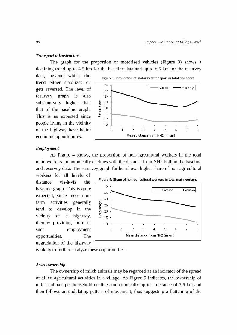
90 Impact Evaluation at Village Level
Transport infrastructure
The graph for the proportion of motorised vehicles (Figure 3) shows a
declining trend up to 4.5 km for the baseline data and up to 6.5 km for the resurvey
data, beyond which the
trend either stabilizes or
gets reversed. The level of
resurvey graph is also
substantively higher than
that of the baseline graph.
This is as expected since
people living in the vicinity
of the highway have better
economic opportunities.
Employment
As Figure 4 shows, the proportion of non-agricultural workers in the total
main workers monotonically declines with the distance from NH2 both in the baseline
and resurvey data. The resurvey graph further shows higher share of non-agricultural
workers for all levels of
distance vis-à-vis the
baseline graph. This is quite
expected, since more non-
farm activities generally
tend to develop in the
vicinity of a highway,
thereby providing more of
such employment
opportunities. The
upgradation of the highway
is likely to further catalyze these opportunities.
Asset ownership
The ownership of milch animals may be regarded as an indicator of the spread
of allied agricultural activities in a village. As Figure 5 indicates, the ownership of
milch animals per household declines monotonically up to a distance of 3.5 km and
then follows an undulating pattern of movement, thus suggesting a flattening of the
Figure 3: Proportion of motorized transport in total transport
Figure 4: Share of non-agricultural workers in total main workers

91 Impact Evaluation at Village Level
curve beyond 3.5 km, on average, in the base year situation. As per the resurvey data,
the value of the variable monotonically rises over distance. This is clearly indicative
of the spatially penetrating effect of highway upgradation. The inter-sectoral linkage
effect may warrant a change in our a priori expectation regarding the nature of such
relationship.
Figure 6, on the
other hand, presents the
graph of the estimated non-
parametric regression for
the proportion of semi-
pucca and pucca houses.
The graph tends to decline
monotonically up to a
distance of around 4 km in
the baseline situation and up
to 3.5 km for the resurvey
situation. It is interesting to
note that the level of the
proportion has been lower
for the resurvey graph up to
4 km, beyond which it has
been higher than the
baseline graph. This again
suggests some higher
beneficial impact on distant
villages between the two
periods, either due to the agrarian development driven by linkage effects on farther
places or due to other developmental factors.
Figure 5: Number of milch animals per household
Figure 6: Proportion of semi-pucca/pucca houses
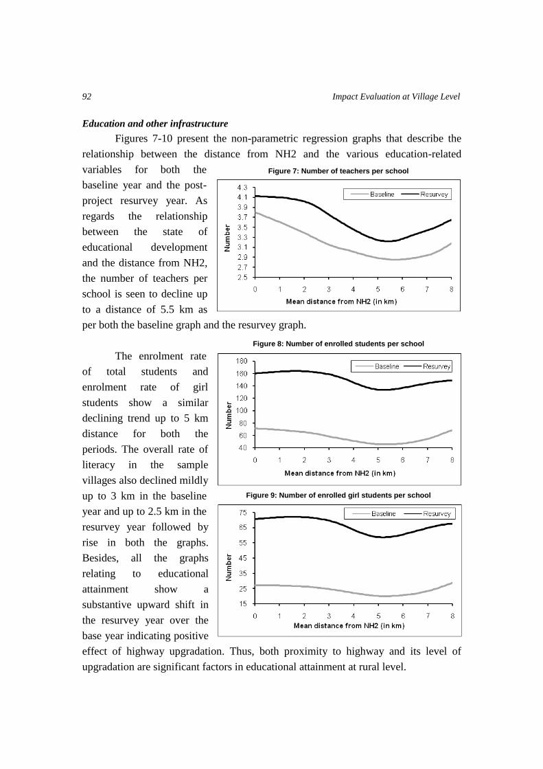
92 Impact Evaluation at Village Level
Education and other infrastructure
Figures 7-10 present the non-parametric regression graphs that describe the
relationship between the distance from NH2 and the various education-related
variables for both the
baseline year and the post-
project resurvey year. As
regards the relationship
between the state of
educational development
and the distance from NH2,
the number of teachers per
school is seen to decline up
to a distance of 5.5 km as
per both the baseline graph and the resurvey graph.
The enrolment rate
of total students and
enrolment rate of girl
students show a similar
declining trend up to 5 km
distance for both the
periods. The overall rate of
literacy in the sample
villages also declined mildly
up to 3 km in the baseline
year and up to 2.5 km in the
resurvey year followed by
rise in both the graphs.
Besides, all the graphs
relating to educational
attainment show a
substantive upward shift in
the resurvey year over the
base year indicating positive
effect of highway upgradation. Thus, both proximity to highway and its level of
upgradation are significant factors in educational attainment at rural level.
Figure 7: Number of teachers per school
Figure 8: Number of enrolled students per school
Figure 9: Number of enrolled girl students per school

93 Impact Evaluation at Village Level
So far as the
availability of banking
facilities is concerned
(Figure 11), the baseline
regression curve declines
monotonically up to 5 km
and considerably flattens
beyond that. The resurvey
curve of regression shows
mild monotonic rise with
distance covering the entire
range of 8.5 km of approach
distance. For the existence
of a cooperative society
(Figure 12), on the other
hand, the baseline regression
graph curve declines
monotonically all through,
while the resurvey graph
shows a rise up to 4 km and
then mildly declines with
distance.
For both the banking
facility and the cooperative
society institutions, the
levels of resurvey graph are
substantially higher than
those of the baseline graph
showing a positive impact of
highway upgradation between the two periods.
Figure 10: Percentage of literate population
Figure 11: Proportion of villages having banking facilities
Figure 12: Proportion of villages having a cooperative society
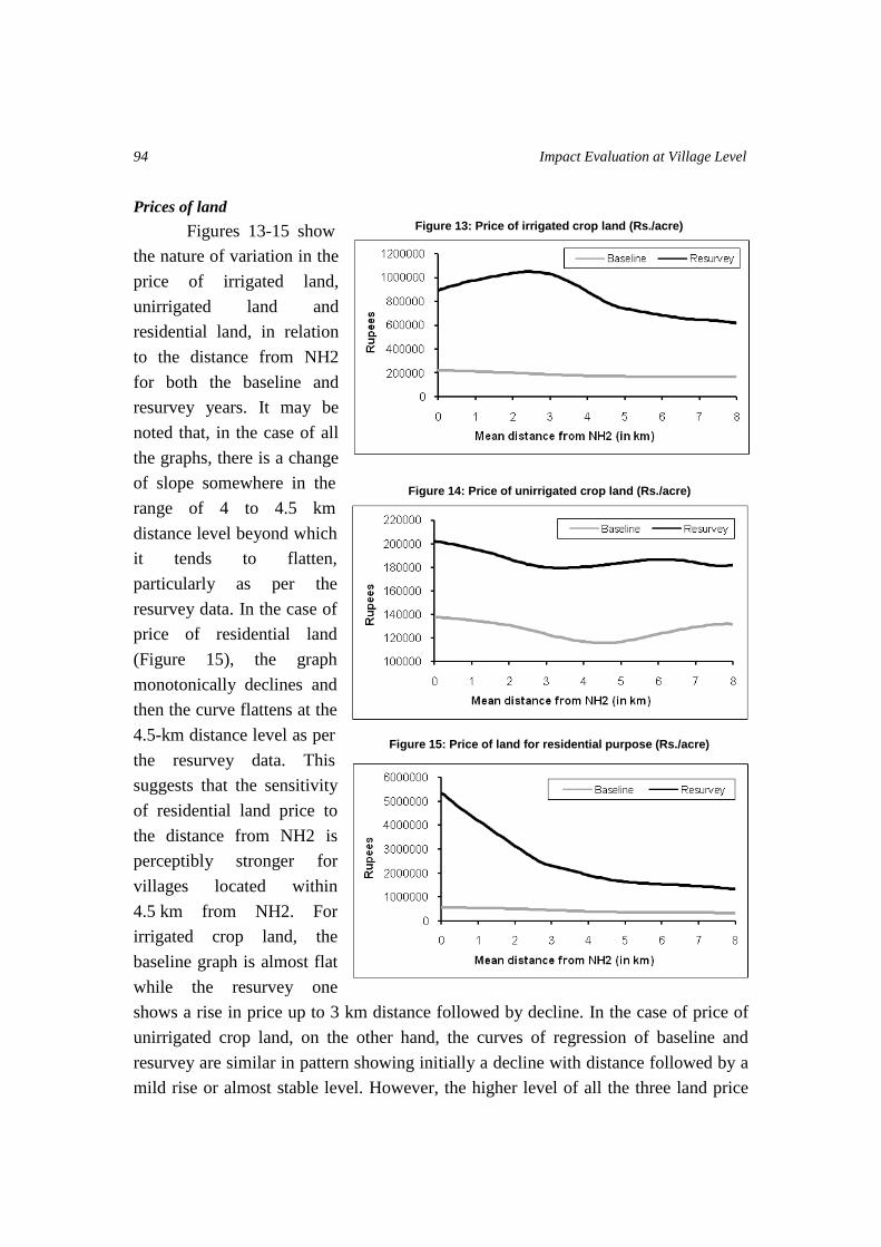
94 Impact Evaluation at Village Level
Prices of land
Figures 13-15 show
the nature of variation in the
price of irrigated land,
unirrigated land and
residential land, in relation
to the distance from NH2
for both the baseline and
resurvey years. It may be
noted that, in the case of all
the graphs, there is a change
of slope somewhere in the
range of 4 to 4.5 km
distance level beyond which
it tends to flatten,
particularly as per the
resurvey data. In the case of
price of residential land
(Figure 15), the graph
monotonically declines and
then the curve flattens at the
4.5-km distance level as per
the resurvey data. This
suggests that the sensitivity
of residential land price to
the distance from NH2 is
perceptibly stronger for
villages located within
4.5 km from NH2. For
irrigated crop land, the
baseline graph is almost flat
while the resurvey one
shows a rise in price up to 3 km distance followed by decline. In the case of price of
unirrigated crop land, on the other hand, the curves of regression of baseline and
resurvey are similar in pattern showing initially a decline with distance followed by a
mild rise or almost stable level. However, the higher level of all the three land price
Figure 13: Price of irrigated crop land (Rs./acre)
Figure 14: Price of unirrigated crop land (Rs./acre)
Figure 15: Price of land for residential purpose (Rs./acre)
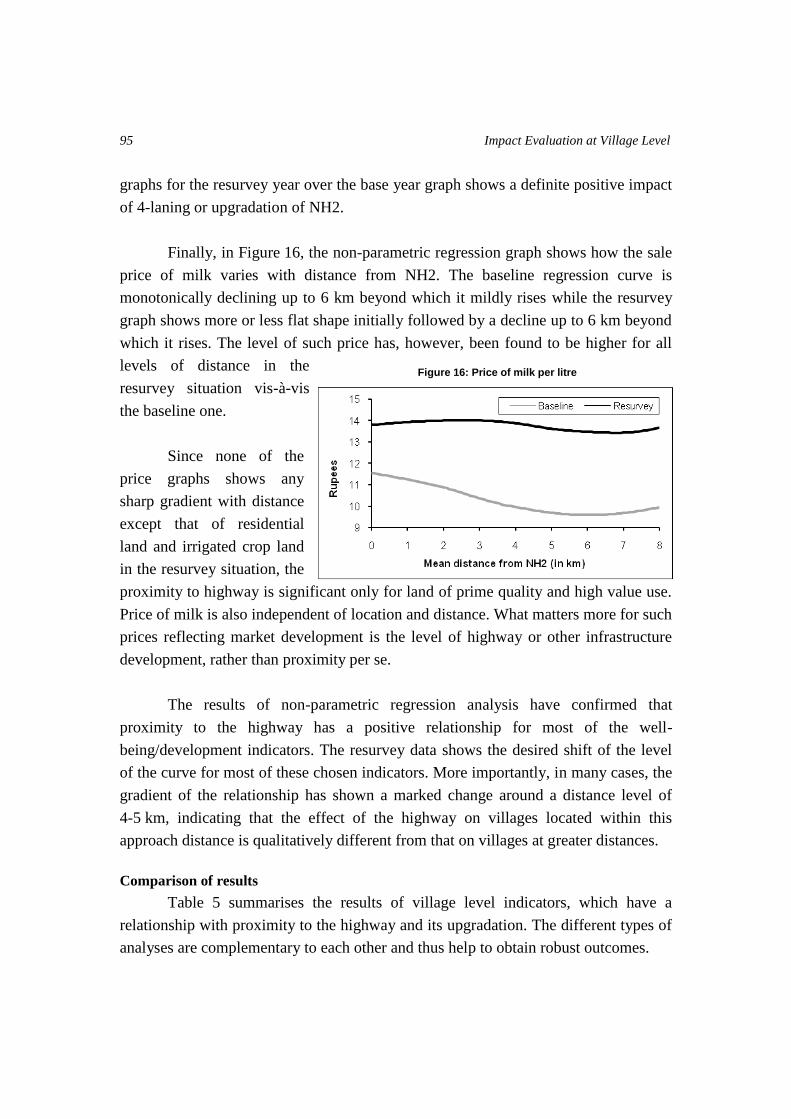
95 Impact Evaluation at Village Level
graphs for the resurvey year over the base year graph shows a definite positive impact
of 4-laning or upgradation of NH2.
Finally, in Figure 16, the non-parametric regression graph shows how the sale
price of milk varies with distance from NH2. The baseline regression curve is
monotonically declining up to 6 km beyond which it mildly rises while the resurvey
graph shows more or less flat shape initially followed by a decline up to 6 km beyond
which it rises. The level of such price has, however, been found to be higher for all
levels of distance in the
resurvey situation vis-à-vis
the baseline one.
Since none of the
price graphs shows any
sharp gradient with distance
except that of residential
land and irrigated crop land
in the resurvey situation, the
proximity to highway is significant only for land of prime quality and high value use.
Price of milk is also independent of location and distance. What matters more for such
prices reflecting market development is the level of highway or other infrastructure
development, rather than proximity per se.
The results of non-parametric regression analysis have confirmed that
proximity to the highway has a positive relationship for most of the well-
being/development indicators. The resurvey data shows the desired shift of the level
of the curve for most of these chosen indicators. More importantly, in many cases, the
gradient of the relationship has shown a marked change around a distance level of
4-5 km, indicating that the effect of the highway on villages located within this
approach distance is qualitatively different from that on villages at greater distances.
Comparison of results
Table 5 summarises the results of village level indicators, which have a
relationship with proximity to the highway and its upgradation. The different types of
analyses are complementary to each other and thus help to obtain robust outcomes.
Figure 16: Price of milk per litre
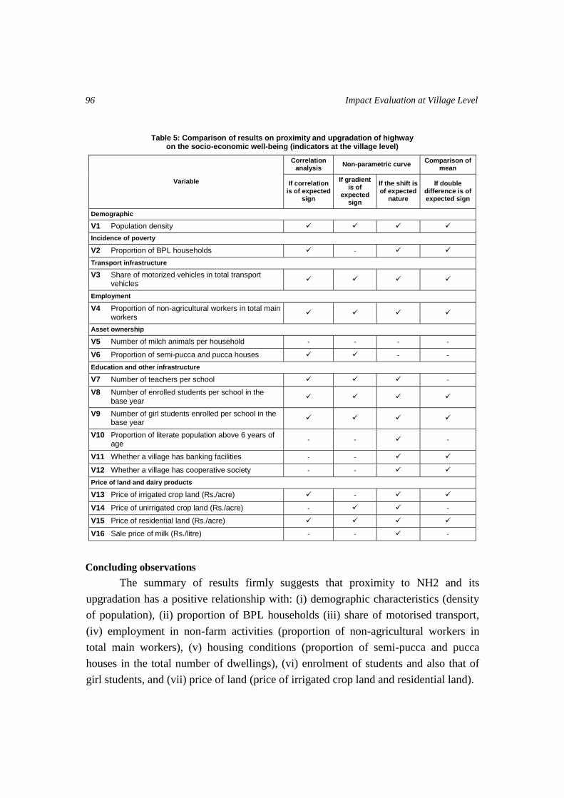
96 Impact Evaluation at Village Level
Table 5: Comparison of results on proximity and upgradation of highway on the socio-economic well-being (indicators at the village level)
Variable
Correlation analysis
Non-parametric curve Comparison of
mean
If correlation is of expected
sign
If gradient is of
expected sign
If the shift is of expected
nature
If double difference is of expected sign
Demographic
V1 Population density
Incidence of poverty
V2 Proportion of BPL households -
Transport infrastructure
V3 Share of motorized vehicles in total transport vehicles
Employment
V4 Proportion of non-agricultural workers in total main workers
Asset ownership
V5 Number of milch animals per household - - - -
V6 Proportion of semi-pucca and pucca houses - -
Education and other infrastructure
V7 Number of teachers per school -
V8 Number of enrolled students per school in the base year
V9 Number of girl students enrolled per school in the base year
V10 Proportion of literate population above 6 years of age
- - -
V11 Whether a village has banking facilities - -
V12 Whether a village has cooperative society - -
Price of land and dairy products
V13 Price of irrigated crop land (Rs./acre) -
V14 Price of unirrigated crop land (Rs./acre) - -
V15 Price of residential land (Rs./acre)
V16 Sale price of milk (Rs./litre) - - -
Concluding observations
The summary of results firmly suggests that proximity to NH2 and its
upgradation has a positive relationship with: (i) demographic characteristics (density
of population), (ii) proportion of BPL households (iii) share of motorised transport,
(iv) employment in non-farm activities (proportion of non-agricultural workers in
total main workers), (v) housing conditions (proportion of semi-pucca and pucca
houses in the total number of dwellings), (vi) enrolment of students and also that of
girl students, and (vii) price of land (price of irrigated crop land and residential land).
97 Impact Evaluation at Village Level
This relationship has brought about a desired shift of the curve for most of the
identified village-level indicators of well-being. Furthermore, the gradient of the
relationship has a marked turning around at a distance of 4-5 km which happens to be
in sync with the hypothesis of the influence zone of the highway on the rural
settlements.
The improved job opportunities available in closer proximity to the highway
have a significant influence on the demographic characteristics in terms of higher
density of population in the nearby villages. In particular, the relatively poor tend to
stay closer to the highway because of better job prospects in non-agricultural
activities and ease of commuting. This phenomenon has implications for interpreting
the gradient of change.

Chapter 5
Impact Evaluation at Household Level
This chapter presents a comprehensive analysis of the household-level data
using different statistical/econometric methods. These methods are complementary to
one another; hence, their simultaneous use may help in getting robust results. The
basic premise underlying the household-level data analysis, as in the case of analysis
of village-level data, is that proximity to NH2 would help improve a household’s
well-being. An improved road infrastructure would further enhance the level of well-
being.
Given that the notion of socio-economic well-being is essentially multi-
dimensional, a wide array of household-level variables (that are likely to reflect the
well-being of the population1) have been analyzed to assess if proximity to NH2 leads
to significant differences in these variables and also to explore the nature of their
individual relationship with distance from NH2. Although poverty is one of the
important manifestations of lack of well-being, the present analysis focuses on other
indicators driving socio-economic well-being at household level.
Four different techniques have been used for the household-level data analysis
– viz., correlation analysis, comparison of means, PSMT2-based single difference
analysis (SDA) and double difference analysis (DDA) and non-parametric regression
analysis (NRA). Of these, the first two constitute the preliminary data analysis.
PSMT-based SDA and DDA have been employed to measure impact by comparing
average values of outcome variables for households in the influence and control
zones. NRA, on the other hand, has been used to explore the nature of relationship of
individual outcome variables with distance from NH2.
Household level variables
As mentioned above, proximity to NH2 is expected to affect a household’s
well-being directly by enhancing mobility and also indirectly by broadening the scope
1. Henceforth, we shall refer to these variables as outcome variables.
2. It may be mentioned here that since the present analysis is based on benchmark survey data, the impact
analysis based on the propensity score matching technique (PSMT) is essentially a single difference analysis
that compares the average value of an outcome variable for households living in the influence zone, i.e. a
defined neighbourhood of NH2 with that of a matched group of households living in the control zone which is
away from NH2.

Impact Evaluation at Household Level 99
for various socio-economic opportunities. To measure these effects, seven different
groups of outcome variables have been considered for the present analysis. These
include a set each of (i) alternative measures of the incidence of poverty, (ii) measures
of mobility, (iii) certain measures of income, employment and occupation, (iv)
variables relating to housing and asset ownership, (v) indicators of access to health,
education and other infrastructural facilities, and (vi) attitudinal variables recording a
household’s perception about its own poverty status and about the possibility of
improvement in the range of its employment opportunities due to the proposed
expansion of NH2. The total number of variables falling under these seven groups is
29. The list of these variables is given in Table 1.
Table 1: List of variables used to study impact of proximity to NH2 based on the household-level data
Incidence of poverty H1* Whether household is poor based on poverty line measured in terms of monthly per capita income (MPCY) H2* Whether household is poor based on poverty line measured in terms of monthly per capita consumption
expenditure (MPCE)
Mobility (weekly) H3 Per capita trip rate (PCTR) H4 Per capita trip rate for work H5 Per capita trip rate for marketing H6 Per capita trip rate for education H7 Per capita trip rate for accessing health-related services H8 Per capita trip rate involving travel on NH2 H9 Per capita trip length for trips involving NH2 H10 Per capita travel expense for trips involving NH2 H11 Per capita travel time for trips involving NH2 H12 Travel cost per person km for trips involving NH2
Income, employment and occupation H13 Per capita income (annual) (Rupees) H14 Per capita consumption expenditure (monthly) (Rupees) H15 Share of income from self-employment in non-agricultural activities H16 Share of food in consumption expenditure H17 Proportion of working members in a household in age group 15-59 years H18 Proportion of working female members in a household in age group 15-59 years H19 Proportion of non-agricultural workers in total working household members.
Asset ownership H20* Whether a household is landless H21* Whether a household owns at least one information related consumer durable (like TV, radio, etc.) H22* Whether a household owns at least one motorised transport vehicle
Education and health H23 Proportion of school-going children among all children in the household in age group 6-14 years H24 Proportion of female school-going children among all female children in the household in age group 6-14
years H25 Proportion of household members who availed of medical facilities during the last six months
Attitudinal response H26* Whether a household rates itself as poor H27* Whether a household expects improvement in employment situation after 4-laning of NH2
Well-being index H28 Index of overall well-being based on income, employment, health and education H29 Index of access to infrastructural facilities, assets and amenities
* These are qualitative binary variables

Socio-economic Impact of National Highway on Rural Population 100
Correlation analysis
For a preliminary analysis, the pattern of interdependence among the chosen
variables has been examined using the simple correlation coefficient between pairs of
variables. The computed correlation matrix is presented in Table 2. It shows that the
correlation with H0 (i.e. distance from NH2) is significant with the expected sign for
eleven variables – H3, H4, H6, H8, H10, H11, H15, H19, H20, H27 and H28.
Importantly, nine of these correlations (viz. all except the ones with H6 and H27)
were also found to be statistically significant in the analysis of baseline survey data. It
also shows that, except in a few cases, the correlation between pairs of chosen
outcome variables is not strong, which suggests that, by and large, the chosen
outcome variables reflect aspects of well-being that are not related to one another.
The pattern of correlation between pairs of outcome variables also provides
certain useful insights. The mobility-related variables per capita trip rate for work
(H4) and per capita trip rate for education (H6) are both positively correlated with per
capita trip rate (H3), suggesting that trips are mostly made for work and education
purposes. The variables H8-H11, all of which involve travel on NH2, are also
positively correlated with one another signifying that proximity to NH2 leads to more
frequent and longer trips.
In the group of variables relating to income, employment and occupation, two
systematic relations may be noticed. The pattern of pair-wise correlation for per capita
income (H13), per capita consumption expenditure (H14) and share of food in
consumption expenditure (H16) are on the expected lines. The correlation between the
proportion of working members in a household in the age group 15-59 years (H17)
and the corresponding variable for working female household members (H18) is also
positive, suggesting that a higher female workforce participation would lead to a
higher overall labour force participation.
The variables relating to education, viz., proportion of school-going children
among children in the age group 6-14 years (H23) and the corresponding variable
relating to education of female children (H24) are highly positively correlated. This is
only to be expected, because a higher schooling rate for female children would push
up the overall schooling rate.
Positive or negative depending on the variable.

Impact Evaluation at Household Level
101 Table 2: Correlation matrix of follow up outcome variables (households)
H0 H1 H2 H3 H4 H5 H6 H7 H8 H9 H10 H11 H12 H13 H14 H15 H16 H17 H18 H19 H20 H21 H22 H23 H24 H25 H26 H27 H28 H29
H0 1.00
H1 -0.01 1.00
H2 -0.01 0.55 1.00
H3 -0.0752* -0.19 -0.17 1.00
H4 -0.0794* -0.03 -0.04 0.60 1.00
H5 0.03 -0.06 -0.06 0.19 -0.31 1.00
H6 -0.0414* -0.16 -0.12 0.49 -0.04 -0.11 1.00
H7 -0.01 -0.06 -0.06 0.11 -0.10 -0.12 -0.03 1.00
H8 -0.1302* -0.09 -0.10 0.56 0.38 0.07 0.21 0.07 1.00
H9 -0.03 -0.06 -0.06 0.10 0.06 -0.07 0.05 0.03 0.21 1.00
H10 -0.0534* -0.06 -0.06 0.05 0.00 -0.04 0.04 0.00 0.09 0.37 1.00
H11 -0.1159* -0.09 -0.10 0.29 0.20 -0.08 0.13 0.06 0.54 0.58 0.28 1.00
H12 0.01 -0.13 -0.10 -0.01 -0.05 -0.02 0.05 -0.01 -0.05 0.05 0.57 0.03 1.00
H13 0.00 -0.20 -0.20 0.11 0.04 0.00 0.08 0.01 0.08 0.10 0.14 0.10 0.09 1.00
H14 -0.01 -0.20 -0.15 0.12 0.01 0.03 0.12 -0.01 0.07 0.09 0.18 0.07 0.13 0.34 1.00
H15 -0.1126* 0.29 0.19 0.03 0.17 -0.07 -0.11 -0.03 0.05 0.01 -0.04 0.04 -0.13 -0.12 -0.11 1.00
H16 0.01 0.39 0.22 -0.12 -0.02 0.04 -0.18 0.00 -0.06 -0.07 -0.15 -0.07 -0.19 -0.26 -0.52 0.14 1.00
H17 0.01 0.10 0.05 0.11 0.16 0.08 -0.13 0.00 0.08 -0.02 -0.05 0.02 -0.06 -0.09 -0.04 0.15 0.04 1.00
H18 0.01 0.05 0.04 0.15 0.12 0.03 0.03 0.00 0.07 -0.02 -0.03 0.03 -0.05 -0.07 -0.03 0.09 -0.03 0.81 1.00
H19 -0.1343* 0.16 0.11 0.02 0.18 -0.12 -0.09 -0.04 0.05 0.01 -0.03 0.03 -0.12 -0.07 -0.07 0.58 0.11 -0.08 -0.20 1.00
H20 -0.0680* 0.25 0.20 0.05 0.14 -0.01 -0.10 0.00 0.01 -0.02 -0.04 -0.03 -0.10 -0.14 -0.15 0.50 0.20 0.21 0.21 0.35 1.00
H21 -0.01 -0.18 -0.16 -0.04 -0.04 -0.09 0.09 -0.06 -0.02 0.02 0.05 -0.01 0.09 0.12 0.09 -0.14 -0.14 -0.16 -0.14 0.00 -0.12 1.00
H22 0.02 -0.33 -0.27 -0.02 -0.07 -0.08 0.12 -0.02 0.01 0.05 0.11 0.02 0.24 0.29 0.30 -0.27 -0.44 -0.20 -0.16 -0.16 -0.29 0.34 1.00
H23 0.00 -0.14 -0.09 -0.01 -0.07 -0.03 0.08 0.01 -0.01 0.03 0.03 0.00 0.07 0.12 0.07 -0.14 -0.11 -0.17 -0.10 -0.12 -0.20 0.08 0.13 1.00
H24 0.01 -0.18 -0.11 0.04 -0.03 -0.03 0.07 -0.01 -0.02 0.02 0.03 -0.01 0.08 0.11 0.06 -0.14 -0.11 -0.16 -0.11 -0.09 -0.18 0.07 0.12 0.90 1.00
H25 -0.02 -0.15 -0.13 0.19 0.03 0.20 0.02 0.15 0.02 -0.03 -0.01 0.00 0.03 0.02 0.02 0.01 -0.05 0.23 0.28 -0.06 0.08 -0.02 -0.10 -0.06 -0.03 1.00
H26 -0.01 0.32 0.27 0.04 0.10 0.06 -0.07 -0.01 0.00 -0.07 -0.05 -0.06 -0.10 -0.17 -0.16 0.32 0.22 0.20 0.17 0.17 0.40 -0.15 -0.36 -0.16 -0.16 0.13 1.00
H27 0.0695* -0.04 0.01 0.01 -0.06 0.09 0.08 -0.05 -0.01 0.00 -0.01 -0.03 0.00 0.06 0.09 -0.21 -0.09 -0.11 -0.09 -0.20 -0.19 0.11 0.18 0.03 0.02 -0.08 0.01 1.00
H28 -0.07* 0.07 0.10 0.10 0.13 0.00 -0.03 0.02 0.04 0.00 0.01 0.03 -0.02 -0.02 0.25 0.57 -0.10 0.53 0.46 0.24 0.31 -0.09 -0.15 0.31 0.24 0.44 0.22 -0.16 1.00
H29 0.01 0.04 0.04 0.03 0.03 -0.03 0.03 -0.02 -0.02 -0.03 0.00 -0.04 -0.01 0.00 0.02 0.03 -0.02 0.04 0.04 -0.01 -0.02 0.00 0.01 0.01 0.02 0.04 0.03 0.06 0.07 1.00
* Significant at 5 percent level with the distance from the highway. H0 denotes approach distance from a household
Socio-economic Impact of National Highway on Rural Population
102
Comparison of means
As a preliminary analysis, whether mean values of individual variables for
influence and control zones are equal has been examined by testing for each variable
the null hypothesis that population means for two zones are equal3. This comparison
of overall means should provide a preliminary idea about the difference in average
levels of the influence and control zones for different variables. Table 3 gives baseline
and resurvey means of the selected outcome variables separately for sample
households falling in influence and control zones, taking the 5 km distance based
delineation of the influence zone. The table also provides (i) the difference of means
of the two zones for baseline survey and resurvey, which should be a crude measure
of the impact of proximity to NH2, and (ii) the difference of these differences, which
should similarly be a crude double difference measure of the impact of upgrading of
NH2.
As Table 3 shows, means of the influence and control zones are different for
10 out of 29 variables for the resurvey data. For 7 out of these 11 variables, the
difference of means is also found for the baseline survey data. These 7 variables are
H3, H4 and H8 related to mobility, H15 and H19 related to income, employment and
occupation, H20 related to asset ownership, and H27 related to attitudinal response.
Significant mean difference is observed for H6, H11 and H25 only for resurvey data
and for H26 only for the baseline survey data. These results thus reinforce the basic
neighbourhood premise for studying the effects of proximity to NH2 on the well-
being of the population.
Comparison of the baseline and resurvey means shows that for 17 out of 29
variables both influence zone and control zone means have improved in the resurvey
data, some of the improvements being fairly large (e.g. trip rate for marketing and
health, proportion of working female members, ownership of information related
consumer durables and motorized transport vehicle, etc.). These improvements in the
means, however, may not be entirely due to the upgrading of NH2.
Finally, the double differences (i.e. the difference of baseline and resurvey
differences of sample means of influence zone and control zone) given in column 7 of
Table 3 suggest the following: For 9 of the 29 outcome variables, this crude measure
of impact of NH2 widening shows expected positive impact, among which are some
related to mobility (H3, H6, H8 and H11), some to income, employment and
occupation (H15 and H19), some to health (H25) and overall wellbeing (H28).
3. The significance of means has been tested using t-test.
Impact Evaluation at Household Level
103
Table 3: Sample mean of outcome variables for influence zone and control zone and their comparison: Baseline survey and resurvey
Variable
Mean value (Baseline)
Baseline difference of
influence zone and
control zone means (1) - (2)
Mean value (Resurvey)
Resurvey difference of
influence zone and
control zone means (4) - (5)
Double difference between
influence zone and control
zone
Percentage increase of
resurvey over the baseline
Influence zone
Control zone
Influence zone
Control zone
1 2 3 4 5 6 7 8
Incidence of poverty
H1 Proportion of poor households based on poverty line measured in terms of MPCY
36.86 38.88 -2.02 31.9 30.31 1.59 3.61 178.71
H2 Proportion of poor households based on poverty line measured in terms of MPCE
45.23 46.73 -1.5 40.83 38.85 1.98 3.48 232.00
Mobility
H3 Per capita trip rate (PCTR) 0.89 0.79 0.09* 1.3 1.16 0.14* 0.05 55.56
H4 Per capita trip rate for work 0.55 0.41 0.14* 0.55 0.43 0.13* -0.01 -7.14
H5 Per capita trip rate for marketing 0.1 0.09 0.01 0.34 0.37 -0.03 -0.04 -400.00
H6 Per capita trip rate for education 0.21 0.25 -0.04 0.28 0.22 0.06* 0.11 250.00
H7 Per capita trip rate for accessing health-related services
0.01 0.02 -0.01 0.06 0.06 -0.01 -0.01 0.00
H8 Per capita trip rate involving travel on NH2 0.42 0.23 0.18* 0.67 0.46 0.21* 0.03 16.67
H9 Per capita trip length for trips involving travel on NH2
3.74 3.28 0.46 6.59 5.15 1.44 0.97 213.04
H10 Per capita travel expenses for trips involving travel on NH2 (Rs.)
1.16 0.94 0.22 5.74 2.29 3.45 3.23 1468.18
H11 Per capita travel time for trips involving travel on NH2 (minutes)
18.18 15.51 2.67 21.6 14.25 7.34* 4.67 174.91
H12 Travel cost per person km for trips involving travel on NH2 (Rs.)
0.000024 0.000042 -0.000018 0.000063 0.000061 0.000002 0.00002
111.11
Income, employment and occupation
H13 Per capita annual income (Rs.) 8143.67 7900.23 243.44 11959.41 12046.93 -87.53 -330.96 -135.96
Deflated per capita annual income (Rs.) 8143.67 7900.23 243.44 8996.84 9053.22 -56.38 -299.81 -123.16
H14 Per capita monthly consumption expenditure (Rs.)
552.79 598.14 -45.34 1101.75 1148.87 -47.12 -1.78 -3.93
Deflated per capita monthly consumption expenditure (Rs.)
552.79 598.14 -45.34 757.95 791.59 -33.64 11.7 25.81
H15 Share of income from self-employment in non-agricultural activities
58.64 54.13 4.51* 58.38 52.98 5.39* 0.88 19.51
H16 Share of food in consumption expenditure 40.59 37.43 3.16 40.33 40.19 0.15 -3.01 -95.25
H17 Proportion of working members in a household in age group 15-59 years
49.43 48.37 1.06 54.24 53.95 0.29 -0.77 -72.64
H18 Proportion of working female members in a household in age group 15-59 years
8.73 8.32 0.41 22.69 22.06 0.64 0.22 56.10
H19 Proportion of non-agricultural workers in total working household members.
56.0442 48.4786 7.57* 63.01 55.27 7.74* 0.17 2.25
Asset ownership
H20 Proportion of landless households 39.4963 35.74701 3.75* 38.1 32.57 5.53* 1.78 47.47
H21 Proportion of households owning at least one information related consumer durable
15.491 15.11748 0.37 70.86 70.74 0.12 -0.25 -67.57
H22 Proportion of households owning at least one motorised transport vehicle
10.5076 11.17186 -0.66 25.31 27.33 -2.01 -1.35 -204.55
Education and health
H23 Proportion of school-going children among all children in age group 6-14 years
82.8477 84.97375 -2.13 90.25 90.62 -0.37 1.75 82.63
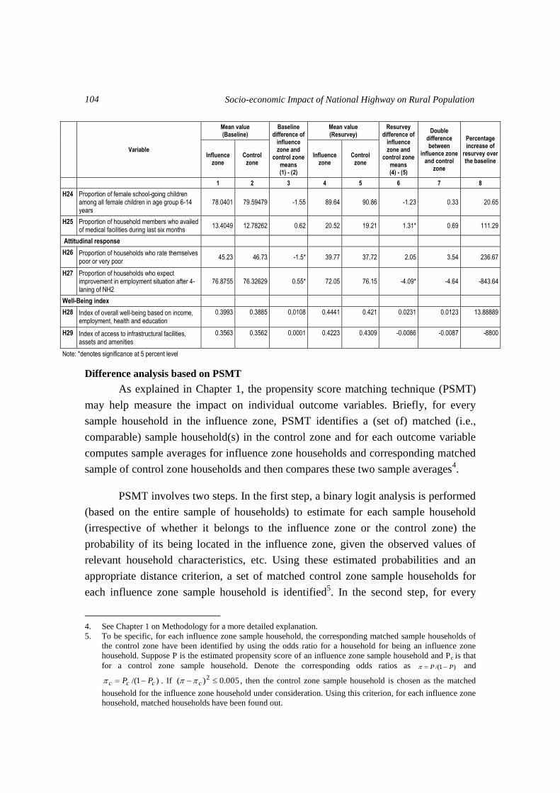
Socio-economic Impact of National Highway on Rural Population
104
Variable
Mean value (Baseline)
Baseline difference of
influence zone and
control zone means (1) - (2)
Mean value (Resurvey)
Resurvey difference of
influence zone and
control zone means (4) - (5)
Double difference between
influence zone and control
zone
Percentage increase of
resurvey over the baseline
Influence zone
Control zone
Influence zone
Control zone
1 2 3 4 5 6 7 8
H24 Proportion of female school-going children among all female children in age group 6-14 years
78.0401 79.59479 -1.55 89.64 90.86 -1.23 0.33 20.65
H25 Proportion of household members who availed of medical facilities during last six months
13.4049 12.78262 0.62 20.52 19.21 1.31* 0.69 111.29
Attitudinal response
H26 Proportion of households who rate themselves poor or very poor
45.23 46.73 -1.5* 39.77 37.72 2.05 3.54 236.67
H27 Proportion of households who expect improvement in employment situation after 4-laning of NH2
76.8755 76.32629 0.55* 72.05 76.15 -4.09* -4.64 -843.64
Well-Being index
H28 Index of overall well-being based on income, employment, health and education
0.3993 0.3885 0.0108 0.4441 0.421 0.0231 0.0123 13.88889
H29 Index of access to infrastructural facilities, assets and amenities
0.3563 0.3562 0.0001 0.4223 0.4309 -0.0086 -0.0087 -8800
Note: *denotes significance at 5 percent level
Difference analysis based on PSMT
As explained in Chapter 1, the propensity score matching technique (PSMT)
may help measure the impact on individual outcome variables. Briefly, for every
sample household in the influence zone, PSMT identifies a (set of) matched (i.e.,
comparable) sample household(s) in the control zone and for each outcome variable
computes sample averages for influence zone households and corresponding matched
sample of control zone households and then compares these two sample averages4.
PSMT involves two steps. In the first step, a binary logit analysis is performed
(based on the entire sample of households) to estimate for each sample household
(irrespective of whether it belongs to the influence zone or the control zone) the
probability of its being located in the influence zone, given the observed values of
relevant household characteristics, etc. Using these estimated probabilities and an
appropriate distance criterion, a set of matched control zone sample households for
each influence zone sample household is identified5. In the second step, for every
4. See Chapter 1 on Methodology for a more detailed explanation.
5. To be specific, for each influence zone sample household, the corresponding matched sample households of
the control zone have been identified by using the odds ratio for a household for being an influence zone
household. Suppose P is the estimated propensity score of an influence zone sample household and Pc is that
for a control zone sample household. Denote the corresponding odds ratios as )1/( PP and
)1/( ccc PP . If 005.0)( 2 c , then the control zone sample household is chosen as the matched
household for the influence zone household under consideration. Using this criterion, for each influence zone
household, matched households have been found out.

Impact Evaluation at Household Level
105
outcome variable, the averages of sample values for the influence zone and the
corresponding control zone matched sample are computed. The difference between
these two computed averages is taken as estimated impact on the particular variable.
The estimated logit model, based on which PSMT has been performed, is presented in
Appendix 1.
It may be noted that the set of explanatory variables of the above-mentioned
estimated logit model mostly include household attributes. Some of these may be
regarded as endogenous variables in the sense that these are partly determined by the
category to which a sample household belongs (in the present case, these categories
are whether a household is in the influence zone or control zone). Normally, such
endogeneity problems of explanatory variables would bias the impact estimator. If the
households had the option to choose their location, the ideal set of explanatory
variables for the logit model would have been the variables inducing that choice.
However, in the present case, households have not chosen their location, but happen
to be located where they are. Since a choice is absent, the cause-effect relationship
between the qualitative dependent variable and whatever explanatory variables are
chosen is bound to be blurred. For example, whether a household is poor because it is
in the control zone or it is in the control zone because it is poor cannot be ascertained.
Given the artificiality of PSMT in the present case, the endogeneity issue appears to
be somewhat ill-defined.
Table 4 gives estimated impact measures obtained as PSMT-based single and
double differences for individual outcome variables, taking the influence zone to be of
5 km distance delineation. It may be noted that the baseline and resurvey (single)
difference between influence zone and control zone given in columns 3 and 6,
respectively, are supposed to measure the impact of proximity to NH2 before and
after upgrading of NH2, and hence the double difference estimate of column 7 is
supposed to be a measure of the impact of upgrading of NH2. It may also be noted
that this procedure of PSMT-based impact measurement through double difference
assumes that (i) upgrading of NH2 is the only intervention and this affects influence
zone alone and (ii) there has been no intervention affecting control zone households
alone6.
6. Clearly these are strong assumptions and their violation will introduce bias in the double difference impact
measures.
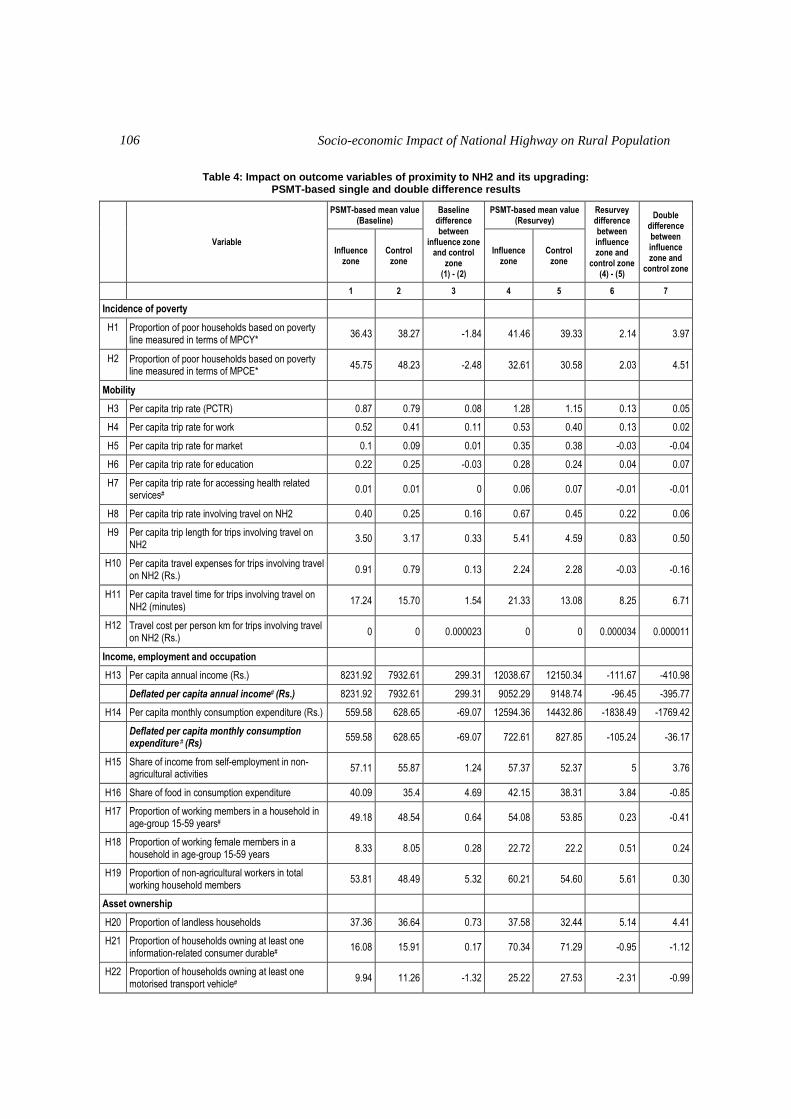
Socio-economic Impact of National Highway on Rural Population
106
Table 4: Impact on outcome variables of proximity to NH2 and its upgrading: PSMT-based single and double difference results
Variable
PSMT-based mean value (Baseline)
Baseline difference between
influence zone and control
zone (1) - (2)
PSMT-based mean value (Resurvey)
Resurvey difference between influence zone and
control zone (4) - (5)
Double difference between influence zone and
control zone
Influence zone
Control zone
Influence zone
Control zone
1 2 3 4 5 6 7
Incidence of poverty
H1 Proportion of poor households based on poverty line measured in terms of MPCY*
36.43 38.27 -1.84 41.46 39.33 2.14 3.97
H2 Proportion of poor households based on poverty line measured in terms of MPCE*
45.75 48.23 -2.48 32.61 30.58 2.03 4.51
Mobility
H3 Per capita trip rate (PCTR) 0.87 0.79 0.08 1.28 1.15 0.13 0.05
H4 Per capita trip rate for work 0.52 0.41 0.11 0.53 0.40 0.13 0.02
H5 Per capita trip rate for market 0.1 0.09 0.01 0.35 0.38 -0.03 -0.04
H6 Per capita trip rate for education 0.22 0.25 -0.03 0.28 0.24 0.04 0.07
H7 Per capita trip rate for accessing health related services#
0.01 0.01 0 0.06 0.07 -0.01 -0.01
H8 Per capita trip rate involving travel on NH2 0.40 0.25 0.16 0.67 0.45 0.22 0.06
H9 Per capita trip length for trips involving travel on NH2
3.50 3.17 0.33 5.41 4.59 0.83 0.50
H10 Per capita travel expenses for trips involving travel on NH2 (Rs.)
0.91 0.79 0.13 2.24 2.28 -0.03 -0.16
H11 Per capita travel time for trips involving travel on NH2 (minutes)
17.24 15.70 1.54 21.33 13.08 8.25 6.71
H12 Travel cost per person km for trips involving travel on NH2 (Rs.)
0 0 0.000023 0 0 0.000034 0.000011
Income, employment and occupation
H13 Per capita annual income (Rs.) 8231.92 7932.61 299.31 12038.67 12150.34 -111.67 -410.98
Deflated per capita annual income# (Rs.) 8231.92 7932.61 299.31 9052.29 9148.74 -96.45 -395.77
H14 Per capita monthly consumption expenditure (Rs.) 559.58 628.65 -69.07 12594.36 14432.86 -1838.49 -1769.42
Deflated per capita monthly consumption expenditure # (Rs)
559.58 628.65 -69.07 722.61 827.85 -105.24 -36.17
H15 Share of income from self-employment in non-agricultural activities
57.11 55.87 1.24 57.37 52.37 5 3.76
H16 Share of food in consumption expenditure 40.09 35.4 4.69 42.15 38.31 3.84 -0.85
H17 Proportion of working members in a household in age-group 15-59 years#
49.18 48.54 0.64 54.08 53.85 0.23 -0.41
H18 Proportion of working female members in a household in age-group 15-59 years
8.33 8.05 0.28 22.72 22.2 0.51 0.24
H19 Proportion of non-agricultural workers in total working household members
53.81 48.49 5.32 60.21 54.60 5.61 0.30
Asset ownership
H20 Proportion of landless households 37.36 36.64 0.73 37.58 32.44 5.14 4.41
H21 Proportion of households owning at least one information-related consumer durable#
16.08 15.91 0.17 70.34 71.29 -0.95 -1.12
H22 Proportion of households owning at least one motorised transport vehicle#
9.94 11.26 -1.32 25.22 27.53 -2.31 -0.99

Impact Evaluation at Household Level
107
Variable
PSMT-based mean value (Baseline)
Baseline difference between
influence zone and control
zone (1) - (2)
PSMT-based mean value (Resurvey)
Resurvey difference between influence zone and
control zone (4) - (5)
Double difference between influence zone and
control zone
Influence zone
Control zone
Influence zone
Control zone
1 2 3 4 5 6 7
Education and health
H23 Proportion of school-going children among all children in age-group 6-14 years
83.21 86.41 -3.20 90.19 91.83 -1.65 1.55
H24 Proportion of female school-going children among all female children in age-group 6-14 years
78.02 82.41 -4.39 89.27 91.83 -2.56 1.83
H25 Proportion of household members who availed of medical facilities during last six months#
13.34 12.68 0.66 19.85 19.74 0.10 -0.56
Attitudinal response
H26 Proportion of households who rate themselves poor or very poor
41.14 42.95 -1.82 39.48 36.74 2.74 4.55
H27 Proportion of households who expect improvement in employment situation after 4-laning of NH2#
78.70 75.46 3.24 73.37 75.42 -2.05 -5.29
Well-Being index
H28 Index of overall well-being based on income, employment, health and education
0.4114 0.4064 0.005 0.4591 0.4371 0.022 0.017
H29 Index of access to infrastructural facilities, assets and amenities#
0.34 0.3398 0.0002 0.4147 0.4204 -0.0057 -0.0059
* : double difference not meaningful # : double difference not expected
The following observations may be made from the data contained in Table 4
above:
In 18 out of 29 cases, the double difference measures show positive impact of
NH2 upgrading. These include all the mobility-related variables except one and 4 of
the 5 employment-related variables (viz. H17 for which the resurvey single difference
has been smaller), those relating to education of both male and female children, and
non-agricultural employment and earning. These are suggestive of perceptible
structural changes taking place in the local economies of the NH2 neighbourhood.
However, there are a few exceptions, notably the one relating to poverty
variables H1 and H2, for which the resurvey means for influence zone are larger7.
This exception could be caused by the effect of simultaneity, omission of which may
introduce bias in double difference impact measures. For example, in the present
impact study, poverty incidence, i.e. probability of a household being poor, is perhaps
7. Note that the poverty incidence increased for both the zones and hence the unexpected result.
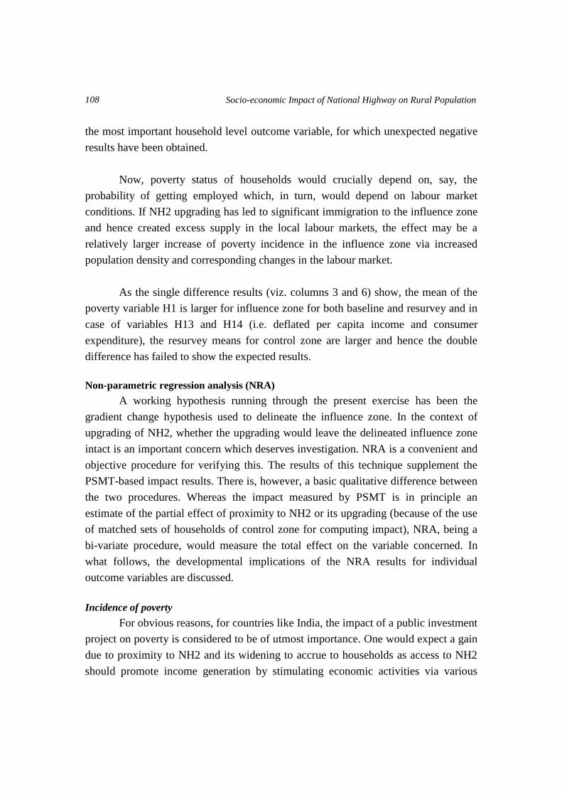
Socio-economic Impact of National Highway on Rural Population
108
the most important household level outcome variable, for which unexpected negative
results have been obtained.
Now, poverty status of households would crucially depend on, say, the
probability of getting employed which, in turn, would depend on labour market
conditions. If NH2 upgrading has led to significant immigration to the influence zone
and hence created excess supply in the local labour markets, the effect may be a
relatively larger increase of poverty incidence in the influence zone via increased
population density and corresponding changes in the labour market.
As the single difference results (viz. columns 3 and 6) show, the mean of the
poverty variable H1 is larger for influence zone for both baseline and resurvey and in
case of variables H13 and H14 (i.e. deflated per capita income and consumer
expenditure), the resurvey means for control zone are larger and hence the double
difference has failed to show the expected results.
Non-parametric regression analysis (NRA)
A working hypothesis running through the present exercise has been the
gradient change hypothesis used to delineate the influence zone. In the context of
upgrading of NH2, whether the upgrading would leave the delineated influence zone
intact is an important concern which deserves investigation. NRA is a convenient and
objective procedure for verifying this. The results of this technique supplement the
PSMT-based impact results. There is, however, a basic qualitative difference between
the two procedures. Whereas the impact measured by PSMT is in principle an
estimate of the partial effect of proximity to NH2 or its upgrading (because of the use
of matched sets of households of control zone for computing impact), NRA, being a
bi-variate procedure, would measure the total effect on the variable concerned. In
what follows, the developmental implications of the NRA results for individual
outcome variables are discussed.
Incidence of poverty
For obvious reasons, for countries like India, the impact of a public investment
project on poverty is considered to be of utmost importance. One would expect a gain
due to proximity to NH2 and its widening to accrue to households as access to NH2
should promote income generation by stimulating economic activities via various

Impact Evaluation at Household Level
109
linkage effects8. To put it differently, between two households with similar attributes
and resource endowments, one located in the influence zone and the other in the
control zone, the probability of the former being poor should be lower as this
household would be able to utilize resource endowments better due to greater
accessibility and mobility provided by its proximity to NH2. Widening of NH2 is
likely to increase the difference of this probability for a household of control zone vis-
à-vis that for an influence zone household.
Given the importance of incidence of poverty as an outcome variable for this
impact study, care has been taken to have this variable measured satisfactorily. As
already mentioned, two different measures of poverty based on MPCY (H1) and
MPCE (H2) are considered here. Note that, whether the MPCY or MPCE should be
used to measure the poverty incidence has been an issue of intense debate in the
country. Use of consumer expenditure data is preferred by many for two reasons – (i)
consumer expenditure relates more directly to nutritional deprivation, which is a
major dimension of absolute poverty, and (ii) compared to income, consumer
expenditure data collected through household survey may be more reliable as a
measure of well-being. Standard arguments put forward in this context relate to
greater recall lapse and the tendency to underreport in case of income.
For MPCE-based poverty variable H2, the official poverty line has been
adopted. Using this, a sample household is classified if its MPCE is found below the
poverty line. The poverty lines for the concerned states given by the Planning
Commission with appropriate indexation for price level changes have been used. The
poverty line in terms of MPCY has been estimated by inverse interpolation. Thus,
using the observed MPCE and MPCY data, a log-linear consumption function is
estimated by regressing the logarithm of MPCE on the logarithm of MPCY. Then the
MPCY corresponding to the given poverty line in terms of MPCE is calculated from
the fitted consumption function. These estimated MPCY values are used as poverty
lines in terms of income.
Figures9 1 and 2 give the NPR graphs for poverty variables H2 and H1,
respectively. One would expect these graphs to rise with distance from NH2 and/or to
8. As mentioned elsewhere, a road development is expected to generate important general equilibrium effects at
the national or state level, in addition to major local effects. In an impact analysis based on household/village-
level data, one may expect to find out these local effects only.
9. Distances are plotted against X-axis for all the figures.

Socio-economic Impact of National Highway on Rural Population
110
be rising after the impact of NH2 has vanished, unless effect of some other
influence/intervention induces a change of gradient. Given this, the shape of these
graphs suggests the following: (1) The influence zone may have changed from 5.5 to
7 km for H1 and from 5.5 to 7 km for H2; and (2) For both H1 and H2, the resurvey
graph is lower at all distances – which is consistent with the expected beneficial
impact of widening of NH2 on poverty incidence.
Figure 1: Proportion of poor households based on poverty line measured in terms of MPCY
Figure 2: Proportion of poor households based on poverty line measured in terms of MPCE
Mobility
The direct economic benefits of proximity to NH2 should arise out of
enhanced mobility of people. A household living close to NH2 should have greater
movement for work, business, education and health, etc. and so a larger per capita trip
rate, compared to a household, otherwise similar, but not having access to NH2. We
Impact Evaluation at Household Level
111
have seen that 6 out of the 10 mobility-related variables, viz. H3, H4, H6, H8, H10
and H11, show significant negative correlation with distance from NH2 for both
baseline and resurvey data and the strength of this correlation has increased between
the surveys for all of them.
Figure 3: Per capita trip rate
Figures 3-12 give the NPR graphs for the 10 mobility-related variables (viz.
H3 to H12). A careful examination of these graphs would suggest the following
conclusions: Mobility has substantially increased after NH2 widening, except for trips
involving direct use of NH2. However, the influence zone limits for most mobility
related variables have remained either between 3.5-4.5 km range or between 5-5.5 km
range and widening of NH2 has, by and large, not strongly affected the influence
zone. Figure 4: Per capita trip rate for work

Socio-economic Impact of National Highway on Rural Population
112
Figure 5: Per capita trip rate for market
Figure 6: Per capita trip rate for education
Figure 7: Per capita trip rate for health
Impact Evaluation at Household Level
113
Figure 8: Per capita trip rate on NH
Figure 9: Per capita trip length on NH
Figure 10: Per capita travel cost on NH

Socio-economic Impact of National Highway on Rural Population
114
Figure 11: Per capita travel time on NH (minutes)
Figure 12: Spending per capita per km on NH (Rs.)
Income, employment and occupation
Proximity to NH2 is likely to promote a structural change towards more
remunerative non-agricultural activities in local economies of the neighbourhood. In
addition, improved connectivity will enable those living closer to NH2 to find more
non-agricultural employment farther away. This implies that income, consumption,
share of non-agricultural income in total income, proportion of non-agricultural
workers in all workers, etc. would be inversely related with the distance of NH2 and
levels of these variables would increase after NH2 upgrading.

Impact Evaluation at Household Level
115
Figure 13: Annual per capita income (Rs.)
Figure 13, which gives the NPR graph for H13 (annual per capita income),
shows broadly the expected inverse relationship with distance from NH2 for both the
baseline and resurvey data. In both cases, a change of gradient with the reversal of
direction is suggested at around 4.5 km distance. This may be taken as the unchanged
limit of the influence zone for this variable. The higher level of the resurvey graph at
all distances may be indicative of the positive effect of NH2 upgrading.
Figure 14: Monthly per capita consumption expenditure (MPCE) (Rs.)
For H14 (MPCE), the baseline and resurvey graphs are of quite different
shapes. Whereas the baseline graph shows a rising tendency up to 5 km and then
declines sharply, the resurvey graph has a tendency to decline all through, attaining a
local minimum around 4 km. Thus, in this case, whereas the baseline graph does not
support the expected inverse relationship of MPCE with distance, the resurvey graph
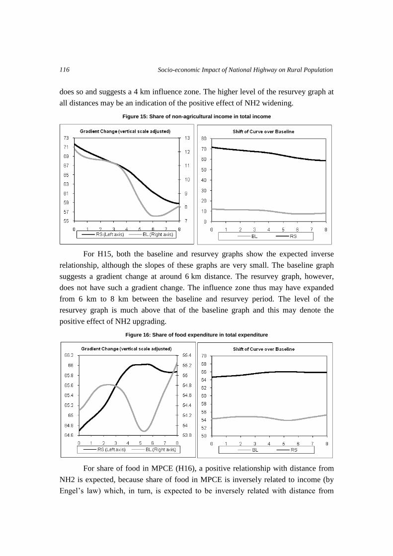
Socio-economic Impact of National Highway on Rural Population
116
does so and suggests a 4 km influence zone. The higher level of the resurvey graph at
all distances may be an indication of the positive effect of NH2 widening.
Figure 15: Share of non-agricultural income in total income
For H15, both the baseline and resurvey graphs show the expected inverse
relationship, although the slopes of these graphs are very small. The baseline graph
suggests a gradient change at around 6 km distance. The resurvey graph, however,
does not have such a gradient change. The influence zone thus may have expanded
from 6 km to 8 km between the baseline and resurvey period. The level of the
resurvey graph is much above that of the baseline graph and this may denote the
positive effect of NH2 upgrading.
Figure 16: Share of food expenditure in total expenditure
For share of food in MPCE (H16), a positive relationship with distance from
NH2 is expected, because share of food in MPCE is inversely related to income (by
Engel’s law) which, in turn, is expected to be inversely related with distance from
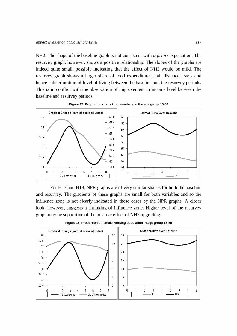
Impact Evaluation at Household Level
117
NH2. The shape of the baseline graph is not consistent with a priori expectation. The
resurvey graph, however, shows a positive relationship. The slopes of the graphs are
indeed quite small, possibly indicating that the effect of NH2 would be mild. The
resurvey graph shows a larger share of food expenditure at all distance levels and
hence a deterioration of level of living between the baseline and the resurvey periods.
This is in conflict with the observation of improvement in income level between the
baseline and resurvey periods.
Figure 17: Proportion of working members in the age group 15-59
For H17 and H18, NPR graphs are of very similar shapes for both the baseline
and resurvey. The gradients of these graphs are small for both variables and so the
influence zone is not clearly indicated in these cases by the NPR graphs. A closer
look, however, suggests a shrinking of influence zone. Higher level of the resurvey
graph may be supportive of the positive effect of NH2 upgrading.
Figure 18: Proportion of female working population in age group 15-59

Socio-economic Impact of National Highway on Rural Population
118
Figure 19: Proportion of non-agricultural workers in total workers
For H19 both the graphs have the expected downward sloping shape over the
entire distance range. The baseline graph, however, shows a very mild gradient
change around 7 km. The resurvey graph having a higher level, is suggestive of a
positive impact of NH2 upgrading.
Assets and ownership
One would expect proximity to NH2 to promote asset acquisition due to
income improvement and NH2 widening should strengthen this tendency. For H20
(probability of being landless), however, appreciation of land value due to proximity
to and/or upgrading of NH2 may induce land sell out and thus H20 may show an
inverse relationship. An inverse relationship with distance from NH2 is also expected
for the other two ownership variables, H21 and H22, due to their positive relation
with income and mobility.
For H20 baseline and resurvey graphs are very similar and monotonically
decreasing. The lower level of the resurvey graph is supportive of positive income
effect of NH2 leading to lower landlessness. The graphs for H21 show a u-shape. The
baseline graph clearly suggests a 4.5 km influence zone. The resurvey graph, which is
much flatter, suggests a 7 km influence zone very weakly. It shows a level about 3
times that of the baseline graph, supporting the positive effect of the NH2 upgrading.
The baseline graph for H22 shows a u-shape. The resurvey graph has a
somewhat different shape with influence zone showing a decline in distance. A higher
level of the resurvey graph could be interpreted as showing the positive effect of NH2
upgrading.
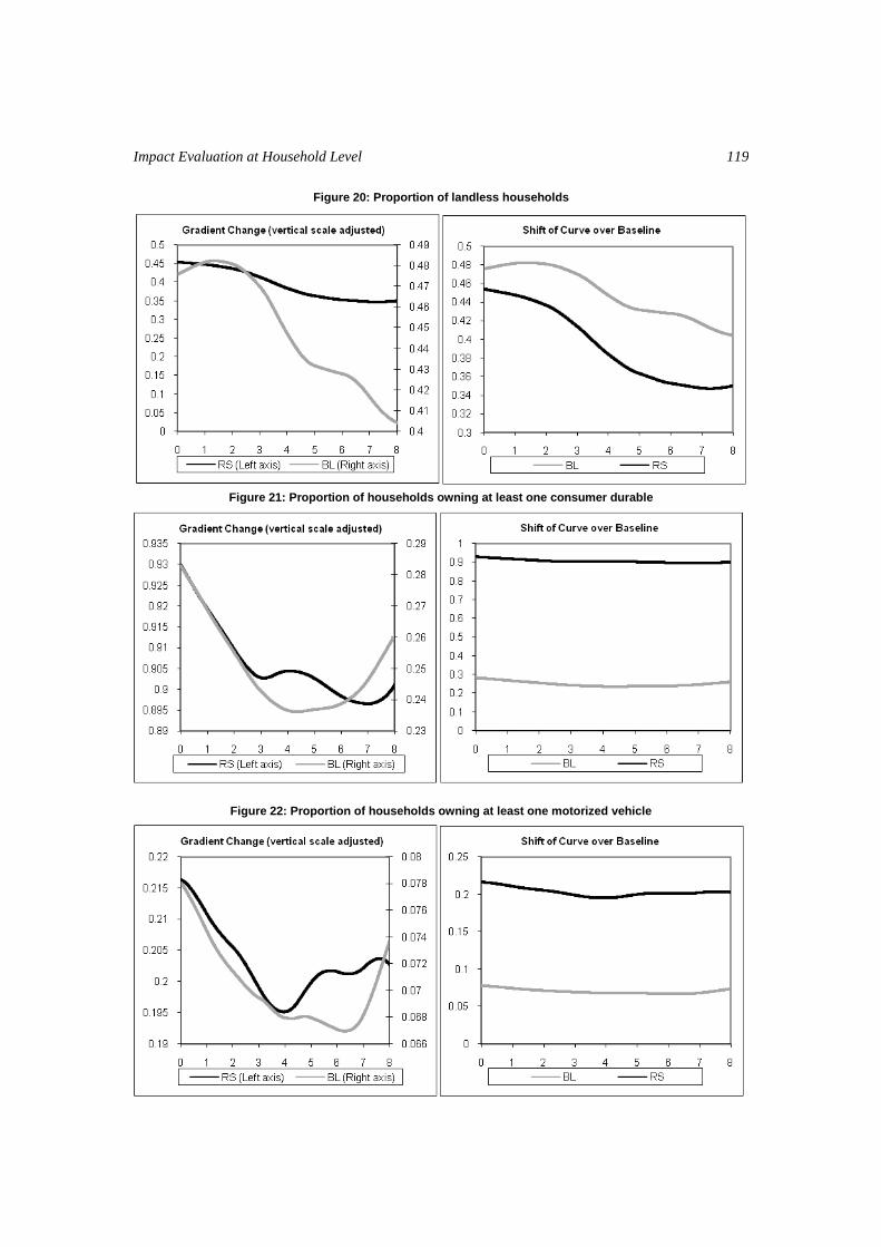
Impact Evaluation at Household Level
119
Figure 20: Proportion of landless households
Figure 21: Proportion of households owning at least one consumer durable
Figure 22: Proportion of households owning at least one motorized vehicle

Socio-economic Impact of National Highway on Rural Population
120
Education and health
Given the expectation that a road infrastructure development would promote
human development, inverse relation of H23 to H25 with NH2 distance is expected
and the level of the function should go up with upgrading of NH2. However, since
these variables are likely to be affected strongly by direct public policy interventions,
shapes of the observed graphs would depend on the pattern of spatial distribution of
such direct public interventions.
The baseline and resurvey graphs for H23 and H24 are of somewhat different
shapes and they do not readily suggest an influence zone. However, in both cases, the
resurvey graph has a higher level. The graphs for both the baseline and resurvey for
H25 decline after an initial phase of approximate constancy. The influence zone
seems to have expanded marginally from 5.5 km to 6 km. The higher level of the
resurvey graph, suggests positive effect of NH2 upgrading.
Figure 23: Proportion of school going children in the age group 6-14 years
Figure 24: Percentage of female school going children in the age group 6-14 years

Impact Evaluation at Household Level
121
Figure 25: Proportion of household members who availed medical services
Attitudinal response
The shapes of the baseline and resurvey graphs of H26 and H27 do not match
the expectation. Since in the case of both of them the baseline and resurvey graphs are
of very dissimilar shapes, it is difficult to conclude much from these graphs. In fact,
the resurvey graph is declining while the baseline graph is rising, which contradicts
expectation.
Figure 26: Proportion of households which rate themselves poor

Socio-economic Impact of National Highway on Rural Population
122
Figure 27: Proportion of household expect improvement in employment
Well-being indices
Finally, the impact of proximity to NH2 has been analyzed in this study for the
two well-being indices: (i) index of overall well-being based on income, employment,
health and education (H28); and (iii) index of well-being in respect of access to basic
amenities like electrical connection, safe drinking water, proper sanitation and type of
house (semi-pucca or pucca) (H29). These indices have been constructed to give an
indication of overall well-being and show the level of socio-economic development.
These indices are the summary measure of well-being and are constructed along the
line of UNDP Human Development Index10
.
The household index of overall well-being has been compiled using the
household specific data on: (a) per capita expenditure, (b) share of income earned
from self-employment in non-agricultural activities, (c) labour participation rate, (d)
proportion of family members visiting health personnel, and (e) proportion of school-
going children. It may be noted that some of these variables are related to entitlement
to well-being [like (a) and (c)], while others relate to capability for well-being [viz.,
(b), (d) and (e)].
The second well-being index, based on access, has been compiled by
combining household specific responses to such qualitative outcome variables as (a)
whether the household has electrical connection, (b) whether it is dependent on
10. See Appendix 1.
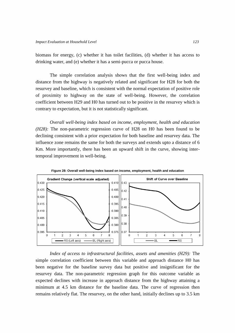
Impact Evaluation at Household Level
123
biomass for energy, (c) whether it has toilet facilities, (d) whether it has access to
drinking water, and (e) whether it has a semi-pucca or pucca house.
The simple correlation analysis shows that the first well-being index and
distance from the highway is negatively related and significant for H28 for both the
resurvey and baseline, which is consistent with the normal expectation of positive role
of proximity to highway on the state of well-being. However, the correlation
coefficient between H29 and H0 has turned out to be positive in the resurvey which is
contrary to expectation, but it is not statistically significant.
Overall well-being index based on income, employment, health and education
(H28): The non-parametric regression curve of H28 on H0 has been found to be
declining consistent with a prior expectation for both baseline and resurvey data. The
influence zone remains the same for both the surveys and extends upto a distance of 6
Km. More importantly, there has been an upward shift in the curve, showing inter-
temporal improvement in well-being.
Figure 28: Overall well-being index based on income, employment, health and education
Index of access to infrastructural facilities, assets and amenities (H29): The
simple correlation coefficient between this variable and approach distance H0 has
been negative for the baseline survey data but positive and insignificant for the
resurvey data. The non-parametric regression graph for this outcome variable as
expected declines with increase in approach distance from the highway attaining a
minimum at 4.5 km distance for the baseline data. The curve of regression then
remains relatively flat. The resurvey, on the other hand, initially declines up to 3.5 km
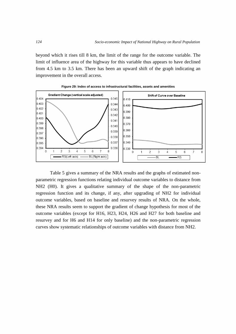
Socio-economic Impact of National Highway on Rural Population
124
beyond which it rises till 8 km, the limit of the range for the outcome variable. The
limit of influence area of the highway for this variable thus appears to have declined
from 4.5 km to 3.5 km. There has been an upward shift of the graph indicating an
improvement in the overall access.
Figure 29: Index of access to infrastructural facilities, assets and amenities
Table 5 gives a summary of the NRA results and the graphs of estimated non-
parametric regression functions relating individual outcome variables to distance from
NH2 (H0). It gives a qualitative summary of the shape of the non-parametric
regression function and its change, if any, after upgrading of NH2 for individual
outcome variables, based on baseline and resurvey results of NRA. On the whole,
these NRA results seem to support the gradient of change hypothesis for most of the
outcome variables (except for H16, H23, H24, H26 and H27 for both baseline and
resurvey and for H6 and H14 for only baseline) and the non-parametric regression
curves show systematic relationships of outcome variables with distance from NH2.
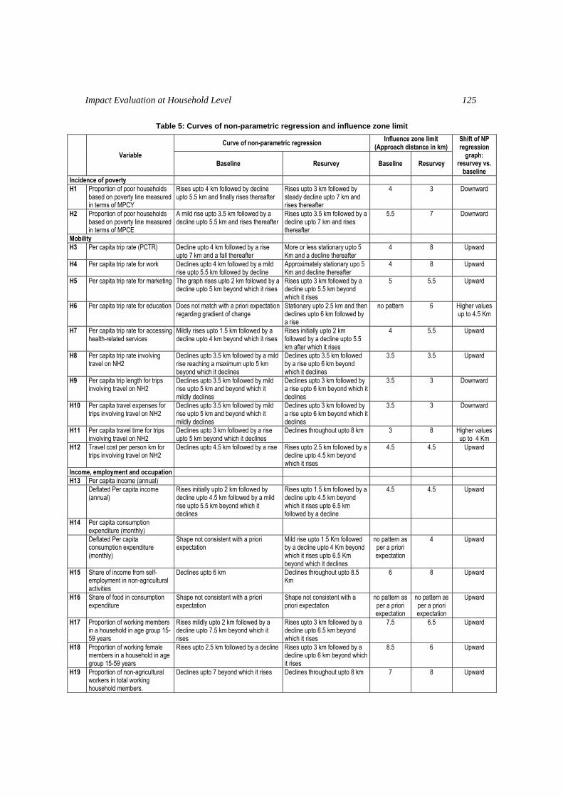
Impact Evaluation at Household Level
125
Table 5: Curves of non-parametric regression and influence zone limit
Variable
Curve of non-parametric regression Influence zone limit
(Approach distance in km) Shift of NP regression
graph: resurvey vs.
baseline Baseline Resurvey Baseline Resurvey
Incidence of poverty
H1 Proportion of poor households based on poverty line measured in terms of MPCY
Rises upto 4 km followed by decline upto 5.5 km and finally rises thereafter
Rises upto 3 km followed by steady decline upto 7 km and rises thereafter
4 3 Downward
H2 Proportion of poor households based on poverty line measured in terms of MPCE
A mild rise upto 3.5 km followed by a decline upto 5.5 km and rises thereafter
Rises upto 3.5 km followed by a decline upto 7 km and rises thereafter
5.5 7 Downward
Mobility
H3 Per capita trip rate (PCTR) Decline upto 4 km followed by a rise upto 7 km and a fall thereafter
More or less stationary upto 5 Km and a decline thereafter
4 8 Upward
H4 Per capita trip rate for work Declines upto 4 km followed by a mild rise upto 5.5 km followed by decline
Approximately stationary upo 5 Km and decline thereafter
4 8 Upward
H5 Per capita trip rate for marketing The graph rises upto 2 km followed by a decline upto 5 km beyond which it rises
Rises upto 3 km followed by a decline upto 5.5 km beyond which it rises
5 5.5 Upward
H6 Per capita trip rate for education Does not match with a priori expectation regarding gradient of change
Stationary upto 2.5 km and then declines upto 6 km followed by a rise
no pattern 6 Higher values up to 4.5 Km
H7 Per capita trip rate for accessing health-related services
Mildly rises upto 1.5 km followed by a decline upto 4 km beyond which it rises
Rises initially upto 2 km followed by a decline upto 5.5 km after which it rises
4 5.5 Upward
H8 Per capita trip rate involving travel on NH2
Declines upto 3.5 km followed by a mild rise reaching a maximum upto 5 km beyond which it declines
Declines upto 3.5 km followed by a rise upto 6 km beyond which it declines
3.5 3.5 Upward
H9 Per capita trip length for trips involving travel on NH2
Declines upto 3.5 km followed by mild rise upto 5 km and beyond which it mildly declines
Declines upto 3 km followed by a rise upto 6 km beyond which it declines
3.5 3 Downward
H10 Per capita travel expenses for trips involving travel on NH2
Declines upto 3.5 km followed by mild rise upto 5 km and beyond which it mildly declines
Declines upto 3 km followed by a rise upto 6 km beyond which it declines
3.5 3 Downward
H11 Per capita travel time for trips involving travel on NH2
Declines upto 3 km followed by a rise upto 5 km beyond which it declines
Declines throughout upto 8 km 3 8 Higher values up to 4 Km
H12 Travel cost per person km for trips involving travel on NH2
Declines upto 4.5 km followed by a rise Rises upto 2.5 km followed by a decline upto 4.5 km beyond which it rises
4.5 4.5 Upward
Income, employment and occupation
H13 Per capita income (annual)
Deflated Per capita income (annual)
Rises initially upto 2 km followed by decline upto 4.5 km followed by a mild rise upto 5.5 km beyond which it declines
Rises upto 1.5 km followed by a decline upto 4.5 km beyond which it rises upto 6.5 km followed by a decline
4.5 4.5 Upward
H14 Per capita consumption expenditure (monthly)
Deflated Per capita consumption expenditure (monthly)
Shape not consistent with a priori expectation
Mild rise upto 1.5 Km followed by a decline upto 4 Km beyond which it rises upto 6.5 Km beyond which it declines
no pattern as per a priori expectation
4 Upward
H15 Share of income from self-employment in non-agricultural activities
Declines upto 6 km Declines throughout upto 8.5 Km
6 8 Upward
H16 Share of food in consumption expenditure
Shape not consistent with a priori expectation
Shape not consistent with a priori expectation
no pattern as per a priori expectation
no pattern as per a priori expectation
Upward
H17 Proportion of working members in a household in age group 15-59 years
Rises mildly upto 2 km followed by a decline upto 7.5 km beyond which it rises
Rises upto 3 km followed by a decline upto 6.5 km beyond which it rises
7.5 6.5 Upward
H18 Proportion of working female members in a household in age group 15-59 years
Rises upto 2.5 km followed by a decline Rises upto 3 km followed by a decline upto 6 km beyond which it rises
8.5 6 Upward
H19 Proportion of non-agricultural workers in total working household members.
Declines upto 7 beyond which it rises Declines throughout upto 8 km 7 8 Upward

Socio-economic Impact of National Highway on Rural Population
126
Variable
Curve of non-parametric regression Influence zone limit
(Approach distance in km) Shift of NP regression
graph: resurvey vs.
baseline Baseline Resurvey Baseline Resurvey
Asset ownership
H20 Proportion of landless households
Rises upto 2.2 km beyond which it declines throughout
Declines upto 7.5 km beyond which it rises
8 7 Marginally lower
H21 Proportion of households owning at least one information related consumer durable
Declines upto 4.5 km followed by a rise Declines upto 7 km followed by a rise
4.5 7 Upward
H22 Proportion of households owning at least one motorised transport vehicle
Declines upto 6.5 km followed by a rise Declines upto 4 km followed by rise of the curve upto 7.5 km beyond which it declines
6.5 4 Upward
Education and health
H23 Proportion of school-going children among all children in age group 6-14 years
Not consistent with a priori expectation and difficulty in conclusion
Not consistent with a priori expectation and difficulty in conclusion
dissimilar shape, no conclusion
dissimilar shape, no conclusion
Upward
H24 Proportion of female school-going children among all female children in age group 6-14 years
Not consistent with a priori expectation and difficulty in conclusion
Not consistent with a priori expectation and difficulty in conclusion
dissimilar shape, no conclusion
dissimilar shape, no conclusion
Upward
H25 Proportion of household members who availed of medical facilities during last six months
Stationary upto 1.5 km followed by a decline upto 5.5 km beyond which it rises
Mildly rises upto 2.5 km followed by a decline upto 6 km beyond which it rises
5.5 6 Upward
Attitudinal response
H26 Proportion of households who rate themselves poor or very poor
Not consistent with a priori expectation and difficulty in conclusion
Not consistent with a priori expectation and difficulty in conclusion
Difficulty in interpretation
Difficulty in interpretation
Inconclusive
H27 Proportion of households who expect improvement in employment situation after 4-laning of NH2
Not consistent with a priori expectation and difficulty in conclusion
Not consistent with a priori expectation and difficulty in conclusion
Difficulty in interpretation
Difficulty in interpretation
Inconclusive
Well-being index
H28 Index of overall well-being based on income, employment, health and education
Declines upto 7 km followed by a rise Declines upto 6.5 km followed by a rise
7 6.5 Upward
H29 Index of access to infrastructural facilities, assets and amenities
Declines upto 4.5 km and remains relatively flat thereafter.
Declines upto 3.5 km follow 4.5 3.5 Upward
As regards the shift of the non-parametric regression curves between baseline
and resurvey, in almost all the cases, the observed shifts indicate improvement, in
some cases substantial improvement, in the level of the outcome variable after
upgrading of NH2. However, it should be noted that since the distance from NH2 is
only one of the sets of explanatory variables influencing the set of outcome variables,
these observed favourable shifts need not be entirely due to the upgrading of NH2.
So far as the expansion of the influence zone of NH2 after its upgrading is
concerned, the results are rather mixed. For some variables (viz. H1, H9, H10, H17,
H18, H20, H22, H28 and H29), a shrink of the influence zone is indicated. For some
others (viz. H2, H3 – H5, H7, H11, H15, H17, H19, H21 and H25), on the other hand,
expansion of the influence zone is suggested. It may be noted in this context that if
the influence zone gets changed, no matter whether it expands or shrinks, the impact
of upgrading would remain somewhat underestimated. This will be so because if the

Impact Evaluation at Household Level
127
influence zone expands (shrinks), the resurvey mean value for the specified control
(influence) zone will overestimate (underestimate) the true control (influence) zone
mean.
PSMT-based impacts – Some recalculations
The NRA results summarized in Table 5 give indication of the possibility that
the influence zone of NH2 may have changed after its upgrading. Normally, in the
absence of any other intervention due to policy or otherwise, the influence zone may
expand, if it changes, and not shrink. The NRA results appear to indicate variable-
specific change of the influence zone in either direction, given the gradient change
criterion used for the purpose of empirical determination of influence zone
delineation. As an illustrative exercise, PSMT-based DDA has been re-done using a
6 km delineation for those 11 outcome variables for which the double difference
impact measures reported in Table 4 turned out to be unexpected and counter-
intuitive. The results of this exercise are given in Table 6.
Table 6: Impact on outcome variables based on comparison of mean values using propensity score
matching of households (6 km limit based influence zone)
Variable
PSMT-based mean value (Baseline)
Baseline difference between influence zone and
control zone (1) - (2)
PSMT-based mean value (Resurvey)
Resurvey difference between
influence zone and control
zone (4) - (5)
Double difference between influence zone and
control zone
Influence zone
Control zone
Influence zone
Control zone
1 2 3 4 5 6 7
Incidence of poverty
H1 Proportion of poor households based on poverty line measured in terms of MPCY
36.6572 38.6705 -2.0134 30.9289 33.8321 -2.9032 -0.8898
H2 Proportion of poor households based on poverty line measured in terms of MPCE
44.6637 50.1217 -5.4580 41.8136 47.7081 -5.8945 -0.4365
Mobility
H7 Per capita trip rate for accessing health related services
0.0131 0.0189 -0.0058 0.0575 0.0644 -0.0069 -0.0011
Income, employment and occupation
H13 Deflated per capita annual income (Rs.) 8151.6456 7884.3683 267.2773 9074.4839 8580.6282 493.8557 226.5784
H14 Deflated per capita monthly consumption expenditure (Rs.)
555.0226 616.9738 -61.9512 780.3302 726.4492 53.8811 115.8323
H17 Proportion of working members in a household in age-group 15-59 years
49.2661 48.6788 0.5873 54.2056 54.2113 -0.0057 -0.5930
Asset ownership
H21 Proportion of households owning at least one information-related consumer durable
15.8744 16.4964 -0.6220 70.7809 71.1305 -0.3497 0.2723
H22 Proportion of households owning at least one motorised transport vehicle
9.9062 12.8578 -2.9516 25.5324 27.6613 -2.1289 0.8227
Education and health
H25 Proportion of household members who availed of medical facilities during last six months
13.1431 13.4933 -0.3502 20.3267 20.3948 -0.0681 0.2821
Attitudinal response
H27 Proportion of households who expect improvement in employment situation after 4-laning of NH2
79.3804 73.6165 5.7638 72.7044 77.4174 -4.7130 -10.4768
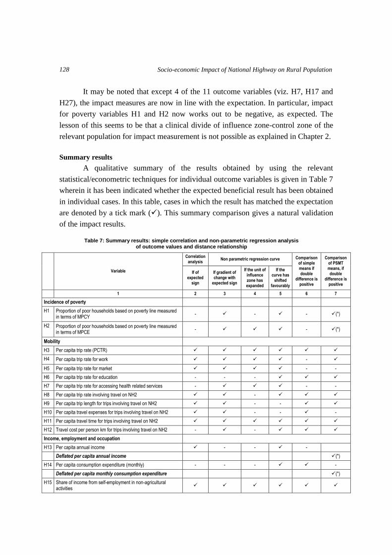
Socio-economic Impact of National Highway on Rural Population
128
It may be noted that except 4 of the 11 outcome variables (viz. H7, H17 and
H27), the impact measures are now in line with the expectation. In particular, impact
for poverty variables H1 and H2 now works out to be negative, as expected. The
lesson of this seems to be that a clinical divide of influence zone-control zone of the
relevant population for impact measurement is not possible as explained in Chapter 2.
Summary results
A qualitative summary of the results obtained by using the relevant
statistical/econometric techniques for individual outcome variables is given in Table 7
wherein it has been indicated whether the expected beneficial result has been obtained
in individual cases. In this table, cases in which the result has matched the expectation
are denoted by a tick mark (). This summary comparison gives a natural validation
of the impact results.
Table 7: Summary results: simple correlation and non-parametric regression analysis
of outcome values and distance relationship
Variable
Correlation analysis
Non parametric regression curve Comparison of simple means if double
difference is positive
Comparison of PSMT means, if double
difference is positive
If of expected
sign
If gradient of change with
expected sign
If the unit of influence zone has expanded
If the curve has
shifted favourably
1 2 3 4 5 6 7
Incidence of poverty
H1 Proportion of poor households based on poverty line measured in terms of MPCY
- - - (*)
H2 Proportion of poor households based on poverty line measured in terms of MPCE
- - (*)
Mobility
H3 Per capita trip rate (PCTR)
H4 Per capita trip rate for work -
H5 Per capita trip rate for market - -
H6 Per capita trip rate for education - - -
H7 Per capita trip rate for accessing health related services - - -
H8 Per capita trip rate involving travel on NH2 -
H9 Per capita trip length for trips involving travel on NH2 - -
H10 Per capita travel expenses for trips involving travel on NH2 - - -
H11 Per capita travel time for trips involving travel on NH2
H12 Travel cost per person km for trips involving travel on NH2 - -
Income, employment and occupation
H13 Per capita annual income - - -
Deflated per capita annual income (*)
H14 Per capita consumption expenditure (monthly) - - - -
Deflated per capita monthly consumption expenditure (*)
H15 Share of income from self-employment in non-agricultural activities
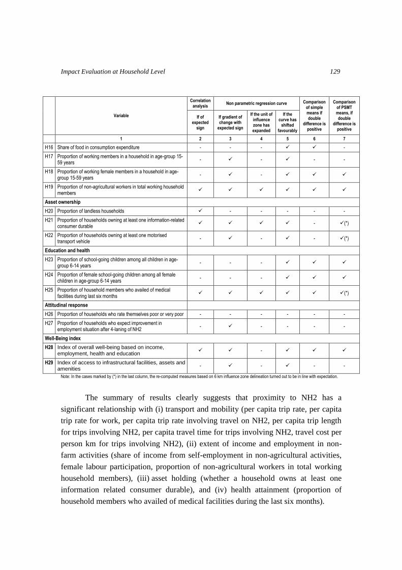
Impact Evaluation at Household Level
129
Variable
Correlation analysis
Non parametric regression curve Comparison of simple means if double
difference is positive
Comparison of PSMT means, if double
difference is positive
If of expected
sign
If gradient of change with
expected sign
If the unit of influence zone has expanded
If the curve has
shifted favourably
1 2 3 4 5 6 7
H16 Share of food in consumption expenditure - - - -
H17 Proportion of working members in a household in age-group 15-59 years
- - - -
H18 Proportion of working female members in a household in age-group 15-59 years
- -
H19 Proportion of non-agricultural workers in total working household members
Asset ownership
H20 Proportion of landless households - - - - -
H21 Proportion of households owning at least one information-related consumer durable
- (*)
H22 Proportion of households owning at least one motorised transport vehicle
- - - (*)
Education and health
H23 Proportion of school-going children among all children in age-group 6-14 years
- - -
H24 Proportion of female school-going children among all female children in age-group 6-14 years
- - -
H25 Proportion of household members who availed of medical facilities during last six months
(*)
Attitudinal response
H26 Proportion of households who rate themselves poor or very poor - - - - - -
H27 Proportion of households who expect improvement in employment situation after 4-laning of NH2
- - - - -
Well-Being index
H28 Index of overall well-being based on income, employment, health and education
-
H29 Index of access to infrastructural facilities, assets and amenities
- - - -
Note: In the cases marked by (*) in the last column, the re-computed measures based on 6 km influence zone delineation turned out to be in line with expectation.
The summary of results clearly suggests that proximity to NH2 has a
significant relationship with (i) transport and mobility (per capita trip rate, per capita
trip rate for work, per capita trip rate involving travel on NH2, per capita trip length
for trips involving NH2, per capita travel time for trips involving NH2, travel cost per
person km for trips involving NH2), (ii) extent of income and employment in non-
farm activities (share of income from self-employment in non-agricultural activities,
female labour participation, proportion of non-agricultural workers in total working
household members), (iii) asset holding (whether a household owns at least one
information related consumer durable), and (iv) health attainment (proportion of
household members who availed of medical facilities during the last six months).

Socio-economic Impact of National Highway on Rural Population
130
As regards the effect on the incidence of poverty, the same has declined in
both the influence and control zones, but the magnitude of reduction has been higher
in the control zone as compared to influence zone. However, the re-estimation of the
net effect based on expansion of the influence zone gave expected positive results.
Concluding observations
Proximity to NH2 and its upgrading has significant beneficial influence on
many aspects of household well-being especially those relating to mobility and non-
agricultural employment, thereby signalling significant structural changes taking
place in the local economies of the neighbourhood of the highway.
The beneficial influence systematically declines as the distance from the
highway increases, thus empirically supporting the gradient change hypothesis. The
influence zone generally extends up to a distance of 4-5 km on either side of the
highway. There are, however, some evidences of the expansion of the influence zone
beyond this distance slab.
Post-upgrading shifts of the NPR curves have mostly been in the expected
direction. This, however, is only suggestive of the positive impact of NH2, as NPR
analysis brings out the total temporal shift of the relationship of an outcome variable
with distance from NH2 rather than the partial shift due to upgrading.
The measured impact of NH2 upgrading based on PSMT-based double
differences is in the expected direction for majority of the outcome variables,
including those for which re-estimation based on 6 km delineation of influence zone
gave expected results.
The presumption of temporal fixity of the delineated influence zone required
for impact measurement based on double difference needs careful attention. It is,
however, realized that a clinical divide of influence zone-control zone for impact
assessment is not possible.
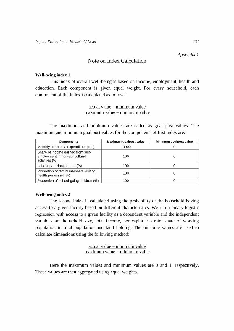
Impact Evaluation at Household Level
131
Appendix 1
Note on Index Calculation
Well-being index 1
This index of overall well-being is based on income, employment, health and
education. Each component is given equal weight. For every household, each
component of the Index is calculated as follows:
actual value – minimum value
maximum value – minimum value
The maximum and minimum values are called as goal post values. The
maximum and minimum goal post values for the components of first index are:
Components Maximum goalpost value Minimum goalpost value
Monthly per capita expenditure (Rs.) 10000 0
Share of income earned from self-employment in non-agricultural activities (%)
100 0
Labour participation rate (%) 100 0
Proportion of family members visiting health personnel (%)
100 0
Proportion of school-going children (%) 100 0
Well-being index 2
The second index is calculated using the probability of the household having
access to a given facility based on different characteristics. We run a binary logistic
regression with access to a given facility as a dependent variable and the independent
variables are household size, total income, per capita trip rate, share of working
population in total population and land holding. The outcome values are used to
calculate dimensions using the following method:
actual value – minimum value
maximum value – minimum value
Here the maximum values and minimum values are 0 and 1, respectively.
These values are then aggregated using equal weights.
Chapter 6
Status of Rural Access and Mobility
Accessibility and mobility are two fundamental aspects of rural road transport.
Accessibility implies ease of access to destinations. Mobility refers to a person’s ability
to travel. Both these aspects have a relationship of reciprocity. Both of them have been
analysed in depth in relation to 200 villages and 3200 households comprising the
universe of the present study.
Concepts of Accessibility and Mobility
The definitions of accessibility and mobility have changed over time and
are often interchangeably used. Mobility is often defined as the amount of
travel people undertake. Accessibility refers to the ability to reach desired
goods, services, activities and destinations. This perspective considers all
access options as potentially important, including motorized and non-
motorized modes. It values modes according to their ability to meet users’
needs, and does not necessarily favour longer trips or faster modes if shorter
trips and slower modes provide adequate access. An important point is the
impact of accessibility on equity. The quality of a person’s or a group’s access
determines their opportunity to engage in economic and social activities.
Policies that favour access for one group over others can be considered
horizontally inequitable.
The analysis covers the status of access from the national highway to the
villages, in particular, the type and nature of this access. It also covers the ownership
pattern of vehicles at the village level and the availability of public transport facilities at
these habitations. The access of the rural population to social infrastructure such as
schools, primary health centres, markets, etc. has also been examined. The issues of
mobility of rural households covering aspects like number of trips performed, travel
time, trip length, etc. have been analyzed extensively.
The thrust of the analysis is to correlate the pattern of travel behaviour in relation
to distance from the highway.It may be mentioned that rural road transport and travel-
related issues have also been discussed in two other chapters of this report. For example,

Status of Rural Access and Mobility
133
the issues relating to the mobility of the poor and disadvantaged population have been
dealt with in Chapter 3, while the relationship between mobility and defined well-being
indicators has been examined in Chapter 5.
Connectivity status
The quality of roads connecting the villages to the national highway has an
important bearing on the optimal use of the highway by the rural population. Figure 1
shows the status of the roads at the
aggregate level connecting all the
200 surveyed villages. The quality of
roads has improved over time. At
present, 84 percent of the villages
have a metalled road access to the
highway.
Table 1 shows the type of
road connectivity in the stretches
falling in the states of Uttar Pradesh,
Bihar and Jharkhand. The quality of
connectivity is better in Uttar Pradesh
as compared to Bihar and Jharkhand.
97 per cent of villages in Uttar
Pradesh are connected to the highway
with at least one metalled road.
Table 2 shows the state-wise
position in respect of the category1 of
road connectivity. As many as 54
villages accounting for 25 percent of
the total villages are connected with
state highways and district roads.
This category of roads, therefore, plays an important role in serving the rural population.
1. In India, the roads are categorized as Village roads, District roads, State highways, National highways.
Table 2: Category of road connectivity at state level (resurvey)
State No. of
villages
Category of road
Village roads
State highways & district
roads
Village, district roads &
state highways
Uttar Pradesh 124 85 36 3
Bihar & Jharkhand 76 53 18 5
Overall 200 138 54 8
Table 1: Type of road connectivity at state level (resurvey)
State No. of
villages
Type of road
Katcha Katcha & metalled
Metalled
Uttar Pradesh 124 4 9 111
Bihar & Jharkhand 76 28 24 24
Overall 200 32 33 135
Figure 1: Distribution of villages by type of roads connecting the highway

Socio-economic Impact of National Highway on Rural Population
134
Vehicle ownership
The rural population own a large variety of vehicles, both motorized and non-
motorized. With the passage of time, the share of motorized vehicles has been
increasing. Table 3 shows the
type and number of vehicles
owned at the village level.
The average ownership per
village works out to 197
vehicles. Bicycles account for
76 percent share. This share
was 87 percent at the time of
the baseline survey. The share
of motorized vehicles has
almost doubled from 8.6
percent to 16 percent. Among
the motorized vehicles, two-
wheelers (motorcycles and
scooters) account for a larger
share.
The distribution of the
share of all types of vehicles
and in particular that of
motorized vehicles in the
distance range of 0-7 km from
the national highway is shown
in Figures 2(a) and 2(b). The
overall vehicle ownership in
close proximity of the highway
(0-1 km) has substantially
declined. However, the
ownership of motorized
vehicles has gone up.
Table 3: Type, number and percentage composition of vehicles
Type of vehicles
Baseline Resurvey
Number Percentage composition
Number Percentage composition
Cycle 33180 87.31 29936 76.08
Cycle rickshaw 227 0.6 1389 3.53
Bullock cart 1061 2.79 1594 4.05
Horse/Camel/Mule cart 128 0.33 134 0.34
Motorcycle 1179 3.1 3921 9.97
Scooter 655 1.72 552 1.4
Three-wheeler 66 0.17 236 0.6
Car/Jeep 250 0.66 295 0.75
Tractor 914 2.41 1085 2.76
Truck 114 0.3 129 0.33
Bus/Minibus 19 0.05 52 0.13
Tempo 32 0.08 8 0.02
Maruta (hybrid vehicle) 25 0.07 16 0.04
Other 153 0.4 0 0
Total 38003 100 39347 100
Figure 2(a): Distribution of share of vehicles by distance from NH2
Table 2(b): Distribution of share of motorized vehicles by distance from NH2

Status of Rural Access and Mobility
135
Public transport facilities
Figure 3 shows the
number of villages having
access to public transport. This
number has increased
significantly since the baseline
survey. At present, 66 percent
of the villages are served by
public transport. The position in
the states of Bihar and
Jharkhand has considerably
improved in this regard.
Approach distance to various
social infrastructure
The ease of accessibility to social infrastructure is an important aspect of
beneficial development. Figure 4 shows average approach distance from villages to
various facilities such as primary school, health centre, local market, etc. Over time,
these basic facilities are getting located closer to the villages, a clear indication of ease
of accessibility to primary social infrastructure.
Figure 4: Average approach distance of villages to social infrastructure
Figure 3: Distribution of villages by availability of public transport facilities
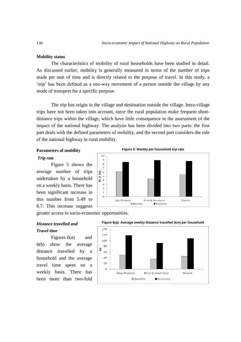
Socio-economic Impact of National Highway on Rural Population
136
Mobility status
The characteristics of mobility of rural households have been studied in detail.
As discussed earlier, mobility is generally measured in terms of the number of trips
made per unit of time and is directly related to the purpose of travel. In this study, a
‘trip’ has been defined as a one-way movement of a person outside the village by any
mode of transport for a specific purpose.
The trip has origin in the village and destination outside the village. Intra-village
trips have not been taken into account, since the rural population make frequent short-
distance trips within the village, which have little consequence in the assessment of the
impact of the national highway. The analysis has been divided into two parts: the first
part deals with the defined parameters of mobility, and the second part considers the role
of the national highway in rural mobility.
Parameters of mobility
Trip rate
Figure 5 shows the
average number of trips
undertaken by a household
on a weekly basis. There has
been significant increase in
this number from 5.49 to
8.7. This increase suggests
greater access to socio-economic opportunities.
Distance travelled and
Travel time
Figures 6(a) and
6(b) show the average
distance travelled by a
household and the average
travel time spent on a
weekly basis. There has
been more than two-fold
Figure 5: Weekly per household trip rate
Figure 6(a): Average weekly distance travelled (km) per household
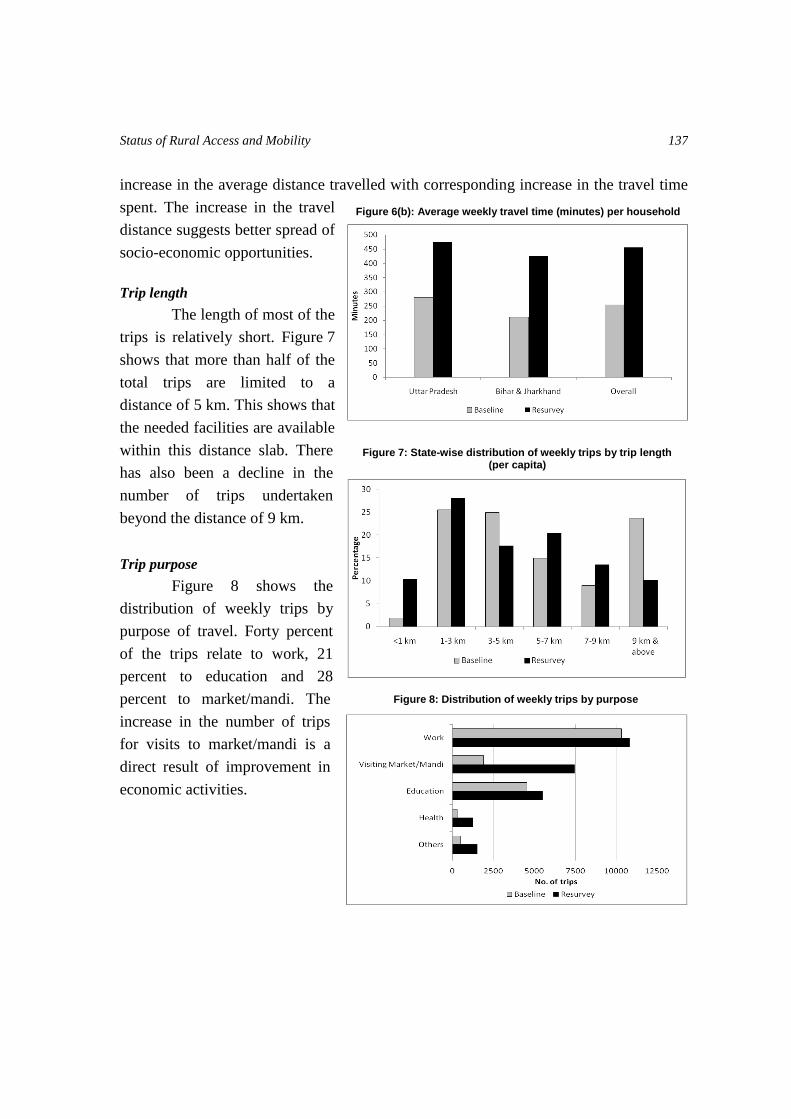
Status of Rural Access and Mobility
137
increase in the average distance travelled with corresponding increase in the travel time
spent. The increase in the travel
distance suggests better spread of
socio-economic opportunities.
Trip length
The length of most of the
trips is relatively short. Figure 7
shows that more than half of the
total trips are limited to a
distance of 5 km. This shows that
the needed facilities are available
within this distance slab. There
has also been a decline in the
number of trips undertaken
beyond the distance of 9 km.
Trip purpose
Figure 8 shows the
distribution of weekly trips by
purpose of travel. Forty percent
of the trips relate to work, 21
percent to education and 28
percent to market/mandi. The
increase in the number of trips
for visits to market/mandi is a
direct result of improvement in
economic activities.
Figure 6(b): Average weekly travel time (minutes) per household
Figure 7: State-wise distribution of weekly trips by trip length
(per capita)
Figure 8: Distribution of weekly trips by purpose
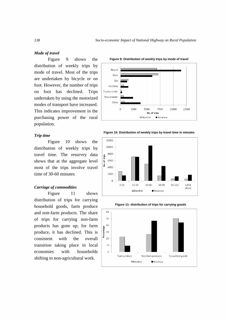
Socio-economic Impact of National Highway on Rural Population
138
Mode of travel
Figure 9 shows the
distribution of weekly trips by
mode of travel. Most of the trips
are undertaken by bicycle or on
foot. However, the number of trips
on foot has declined. Trips
undertaken by using the motorized
modes of transport have increased.
This indicates improvement in the
purchasing power of the rural
population.
Trip time
Figure 10 shows the
distribution of weekly trips by
travel time. The resurvey data
shows that at the aggregate level
most of the trips involve travel
time of 30-60 minutes.
Carriage of commodities
Figure 11 shows
distribution of trips for carrying
household goods, farm produce
and non-farm products. The share
of trips for carrying non-farm
products has gone up; for farm
produce, it has declined. This is
consistent with the overall
transition taking place in local
economies with households
shifting to non-agricultural work.
Figure 9: Distribution of weekly trips by mode of travel
Figure 10: Distribution of weekly trips by travel time in minutes
Figure 11: distribution of trips for carrying goods
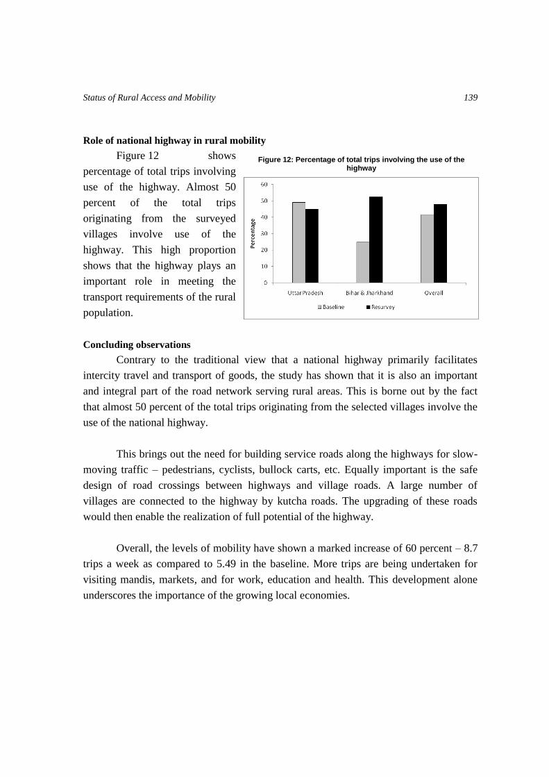
Status of Rural Access and Mobility
139
Role of national highway in rural mobility
Figure 12 shows
percentage of total trips involving
use of the highway. Almost 50
percent of the total trips
originating from the surveyed
villages involve use of the
highway. This high proportion
shows that the highway plays an
important role in meeting the
transport requirements of the rural
population.
Concluding observations
Contrary to the traditional view that a national highway primarily facilitates
intercity travel and transport of goods, the study has shown that it is also an important
and integral part of the road network serving rural areas. This is borne out by the fact
that almost 50 percent of the total trips originating from the selected villages involve the
use of the national highway.
This brings out the need for building service roads along the highways for slow-
moving traffic – pedestrians, cyclists, bullock carts, etc. Equally important is the safe
design of road crossings between highways and village roads. A large number of
villages are connected to the highway by kutcha roads. The upgrading of these roads
would then enable the realization of full potential of the highway.
Overall, the levels of mobility have shown a marked increase of 60 percent – 8.7
trips a week as compared to 5.49 in the baseline. More trips are being undertaken for
visiting mandis, markets, and for work, education and health. This development alone
underscores the importance of the growing local economies.
Figure 12: Percentage of total trips involving the use of the highway
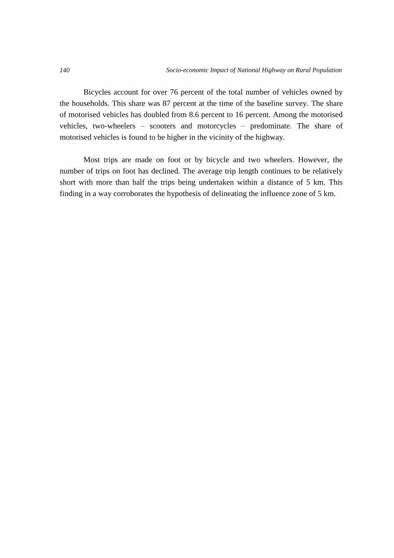
Socio-economic Impact of National Highway on Rural Population
140
Bicycles account for over 76 percent of the total number of vehicles owned by
the households. This share was 87 percent at the time of the baseline survey. The share
of motorised vehicles has doubled from 8.6 percent to 16 percent. Among the motorised
vehicles, two-wheelers – scooters and motorcycles – predominate. The share of
motorised vehicles is found to be higher in the vicinity of the highway.
Most trips are made on foot or by bicycle and two wheelers. However, the
number of trips on foot has declined. The average trip length continues to be relatively
short with more than half the trips being undertaken within a distance of 5 km. This
finding in a way corroborates the hypothesis of delineating the influence zone of 5 km.
Concepts and Definitions
The concepts and definitions of some of the important terms used in the baseline survey
schedules or referred to in the present report are explained below. The technical terms have been
explained, only with a view to enabling the lay reader to understand the context of the narration.
Access: It is the ability to reach, visit, or use a service, and encompasses two factors of mobility and
proximity.
Accessibility: It is a term often used in transport and land use planning and is generally understood to
mean ‘ease of reaching’ (Jones, 1981).
Acre: A unit of surface area (equivalent to 4047 sq.m.)
Agricultural Labour: A person is considered as agricultural labour, if he/she follows one or more of
the following agricultural occupations in the capacity of a wage-paid manual labour, whether paid in
cash or kind or both: (i) farming, (ii) dairy farming, (iii) production of any horticultural commodity,
(iv) raising of livestock, bee-keeping or poultry farming, (v) any practice performed on a farm as
incidental to or in conjunction with farm operations (including forestry and timbering), preparation for
market and delivery to storage or to market or to carriage for transportation to market of farm produce.
Working in fisheries is excluded from agricultural labour. Further, ‘carriage for transportation’ refers
only to the first stage of transport from farm to the first place of disposal. (Source: NSSO)
Agricultural Marketing Societies: These societies are formed by groups of farmers with the objective
of getting better prices for their products. Their activities include collection, processing, selling, and
transporting the products of their members.
Agricultural Production: An occupation category which includes growing of (i) cereal crops (paddy,
wheat, jowar, bajra, maize, ragi, barley, etc.), (ii) pulses (arhar, gram, moong, urad, etc.), (iii) cotton,
(iv) jute, mesta, sann hemp or other kindred fibres, (v) oilseeds, (vi) sugarcane or sugar beet, (vii) roots
and tubers, vegetables, singharas, chillies and spices (other than pepper and cardamom), (viii) fodder
crops; floriculture and horticulture including tree nurseries; and agricultural production not elsewhere
classified. (Source: Census of India)
Agro-climatic Zone: A division of the country based on physical and climatic considerations for an
optimum farming system of crop production. The agro-climatic division (zoning) broadly takes into
account the soil characteristics, climate, rainfall, and water availability. The country has been divided
into 15 zones for the purposes of national agricultural economy:
(i) Western Himalayan (ii) Eastern Himalayan (iii) Lower Gangetic Plains
(iv) Middle Gangetic Plains (v) Upper Gangetic Plains (vi) Trans- Gangetic Plains
(vii) Eastern Plateau and Hills (viii) Central Plateau and Hills (ix) Western Plateau and Hills
(x) Southern Plateau and Hills (xi) East Coast Plains and Hills (xii) West Coast Plains and Ghats
(xiii) Gujarat Plains and Hills (xiv) Western Dry (xv) Islands
(Source: Planning Commission)
Arithmetic Mean or Mean: It is the sum of a set of numbers divided by the number of cases in the set.
It is denoted as X = ( X)/N.
Artisans: An occupation category which includes (i) sculptors, painters and related artists; (ii)
commercial artists, interior decorators and designers; (iii) movie camera operators; (iv) photographers;
(v) composers, musicians and singers; (vi) choreographers; (vii) actors; (viii) stage and film directors
and producers (performing arts); (ix) circus performers (excluding rope dancers and acrobats); (x)
dancers; (xi) rope dancers; (xii) acrobats; and (xiii) snake charmers. (Source: Census of India)
Attached Labour: Contract labour for a specified period of agricultural season.
Socio-economic Impact of National Highway on Rural Population
142
Average Cost: Cost per unit of output, where the costs of all inputs (factors of production) are included.
Thus, the average cost (AC) may be written as: AC = (TC/X), where X is output and TC is the total
cost. Average cost comprises average fixed cost (AFC) and average variable cost (AVC).
Average Daily Traffic (ADT): Average number of vehicles that pass a specified point during a 24-hour
period.
Average Travel Cost: It is the average cost of travel taking all trips into account; also expressed as a
ratio of total trips to total cost.
Average Travel Time: It is the average time of travel taking all trips into account; also expressed as the
ratio of total trips to total travel time.
Average Trip Length: It is the average distance of travel taking all trips into account.
Bias: It may be said to exist when the value of a sample statistics shows a persistent tendency to
deviate in one direction from the value of the parameter.
Big Business (Organised Sector Enterprise): It refers to those enterprises which are registered under
the Factory Act, 1948, and have 10 or more employees, using power for their operations; or have 20 or
more employees and carry out their operations without power (Source: CSO).
Bigha: One fifth of an acre (equivalent to 809 sq.m.)
Casual Wage Labour: A person who is casually engaged in others’ farm or non-farm enterprises (both
household and non-household) and, in return, receives wages according to the terms of the daily or
periodic work contract. Usually, in the rural areas, a type of casual labourers can be seen who normally
engage themselves in ‘public works’ activities. ‘Public works’ are those activities which are sponsored
by the government or local bodies for constructing roads, bunds, digging ponds, etc. as ‘test relief’
measures (like flood relief, drought relief, or famine relief.) and also employment-generation schemes
under poverty alleviation programmes (NREP, RLEGP, etc.). (Source: NSSO)
Co-efficient of Variation (CV): The coefficient of variation is defined as: CV = 100x
, where σ is
the standard deviation and x is the mean. It is used to compare two or more series where the means
differ significantly and where the standard deviation is an inadequate measure of dispersion.
Community Health Centre: It is an upgraded primary health centre provided in each community
development block, covering a population of one lakh. It has up to 30 beds and is equipped with X-ray
and other laboratory facilities. The centre has a specialist each in surgery, medicine, obstetrics,
gynaecology, and pediatrics.
Community Water Supply: Irrigated water supply for a group of people living in a particular area.
Community Wells: Wells dug for the purpose of providing drinking water to a group of people living
in a particular area.
Confidence Interval: It is a random interval for a parameter constructed from data in such a way that
the probability of that interval contains the true value of the parameter which can be specified before
the data are collected.
Confidence Level: It is the chance that the interval which will result once data are collected will
contain the corresponding parameter in a confidence interval. If one computes confidence intervals
again and again from independent data, the long-term limit of the fraction of intervals that contain the
parameter is the confidence level.
Construction Worker(s): Workers classified under this category are: (i) bricklayers, stone masons and
tile-setters; (ii) reinforced concreters, cement finishers and terrazzo workers; (iii) roofers (iv) parquetry
Concepts and Definitions 143
workers; (v) plasterers; (vi) insulators; (vii) glaziers; (viii) hut builders and thatchers; and (ix) well
diggers. (Source: Census of India)
Consumer Price Index: A measurement of average changes in prices paid by consumers of a fixed
basket of a wide variety of goods and services (Source: CSO).
Control Zone (Control Area): It is the area which will be least influenced by the impact of the project.
The control zone enables comparison with the influence zone for the purpose of assessing the net socio-
economic impact of the project. This comparison is done under two situations – before and after the
implementation of the project – so as to isolate the effects of other simultaneous development
initiatives or processes (for the current study, the control zone is the area extending beyond an
approach distance of 5 km within the horizontal distance band of 7 km on either side of the national
highway).
Co-operative: A business owned by people who use its services. Some cooperatives sell goods or
services produced by their members. In the case of other cooperatives, farmers and other consumers as
a group buy directly from suppliers. By reducing expenses, these organisations often provide lower
costs for consumers and higher earnings for producers.
Correlation Coefficient: Given a pair of related measures (X and Y) on each of a set of items, the
correlation coefficient (r) provides an index of the degree to which the paired measures co-vary in a
linear fashion.
Cost-Benefit Analysis: The appraisal of an investment project which includes all social and financial
costs and benefits accruing to the project. It is the technique adopted in investment appraisal in order to
evaluate and decide whether a proposed project should proceed, i.e. its benefits would exceed its costs.
Cross-section Data: A set of data which are collected at one point of time.
Cultivation: All activities related to crop production including ancillary activities are considered as
cultivation. Growing trees, plants, vegetables or of crops as plantation or orchards (such as rubber,
cashew, coconut, pepper, coffee, tea, etc.) is not considered as cultivation activity. (Source: NSSO)
Cultivator: A cultivator is one engaged as employer, single worker or family worker in cultivation of
crops on land owned or held from government or private persons for payments in money, kind or share.
(Source: Census of India)
Degrees of Freedom: This term is used to describe the number of values in the final calculation of a
statistic that are free to vary.
Demand: It is the desire for a commodity backed by ability and willingness to pay.
Development Block: An administrative unit coterminous with the jurisdiction of Panchayat Samiti.
Dhaba: A small open eating place on the roadside, offering inexpensive eatables.
District Rural Development Agency: It is the government nodal agency at the district level which
supports and finances micro development projects in the field of land and water resources.
Double Difference Method: A method of assessing the socio-economic impact of a project (Explained
in detail in the text).
Drought: A situation when the deficiency of rainfall at a meteorological sub-division level is 25
percent or more of the long-term average of that sub-division for a given period. The drought is
considered ‘moderate’, if the deficiency is between 26 and 50 percent, and ‘severe’ if it is more than 50
percent.
Dummy Variable: A binary (off-on) variable designed to take account of exogenous shifts (shift
dummy) or changes of slope (slope dummy) in an econometric relationship. For instance, dummies can
Socio-economic Impact of National Highway on Rural Population
144
be used to account for seasonal influences in the data. By specifying a dummy to take on the value of
unity of, say, winter months, and zero at other times, it will indicate the degree to which a relationship
shifts during the winter, compared to other seasons, by augmenting the constant term of the equation.
This type of variable can also be used to include qualitative factors in a regression.
Economic Activity: Any activity resulting in the production of goods and services that add value to
national product is considered economic activity. Such activities include producing goods and services
for the market (market activities), i.e. production for pay or profit, and the production of primary
commodities for own consumption and own account production of fixed assets, among the non-market
activities. (Source: NSSO)
Economic Development: The process of improving the standard of living and well-being of the
population by raising per capita income.
Economic Growth: Typically taken to mean an increase in the real level of net national product. The
measure is sensitive to the way in which national product is measured. Thus, an economy with a large
sector containing bartered goods or unrecorded consumption of its own products (e.g., farmers’
consumption of their own produce) may raise its level of national product without the recorded level
showing an increase.
Economies of Scale: Reduction in the average cost of a product in the long run, resulting from an
expanded level of output. Also known as long-run increasing returns.
Elasticity of Demand: It is the proportionate change in demand due to change in price.
Employed: See ‘Worker(s)’.
Employee: A worker who is hired to perform a job.
Employment: The state of being employed or having a job (Source: NSSO).
Endogenous Variable: A variable whose value is determined within the framework of an economic or
econometric model. Thus, if a variable appears as a dependent variable in an equation, it is an
endogenous variable.
Enterprise: It is an undertaking which is engaged in the production and/or distribution of some goods
and/or services meant mainly for the purpose of sale, whether fully or partly. An enterprise may be
owned and operated by a single household, or by several households jointly, or by an institutional
body. (Source: NSSO)
Establishment: Those enterprises which have got at least one hired worker on a ‘fairly regular basis’
are called establishments. (Source: NSSO)
Exogenous Variable: A variable whose value is not determined within an economic model, but which
plays a role in the determination of the values of endogenous variable. Thus, an exogenous variable is
an explanatory variable but never appears as a dependent variable in the model.
Explanatory Variable: A variable which plays a part in ‘explaining’ the variation in a dependent
variable in a regression analysis.
Expressway: A highway with divided carriageway, controlled access, generally provided with grade
separations at intersections and permitting only fast-moving vehicles.
Externalities: Externalities are variously known as external effects, external economies and
diseconomies, spillovers and neighbourhood effects. Externalities involve an interdependence of utility
and/or production function. For example, the upstream pulp mill which discharges effluent in the river,
thus reducing the scope of fishing downstream, is said to impose an externality on the fishermen. A
beneficial externality, known as an external economy, is where an externality-generating activity raises
the production or utility of the externally-affected party. For example, a beekeeper may benefit

Concepts and Definitions 145
neighbouring farmers by incidentally supplying pollination services. An external diseconomy is where
the externality-generating activity lowers the production or utility of the externally-affected party.
Examples of this are the numerous forms of environmental pollution.
Factor Analysis: An analytical technique for identifying the major inter-relationships between
variables, frequently used in transportation demand analysis.
Factors of Production: The resources used in the process of production. These are usually divided into
three main groups – land, labour, capital – but may also include entrepreneurship.
Financial Institution(s): It includes any bank, thrift institution, insurance company, investment
advisory firm.
Firm: Analytical label for an institution which transforms inputs into output. Thus, a firm is viewed as
an abstract entity which mainly fulfils technical role.
Fishing: An occupation category which includes: (i) ocean, sea and coastal fishing; (ii) inland water
fishing; (iii) pisciculture: rearing of fish, including fish hatcheries; (iv) collection of pearls, conches,
shells, sponges and other sea products; (v) cultivation of oysters for pearls; and (vi) other allied
activities and services incidental to fishing not elsewhere classified. (Source: Census of India)
Flood: The rising of a body of water and its overflowing on to normally dry land.
Forestry: An occupation category which includes: (i) planting, replanting and conservation of forests;
(ii) logging, felling and cutting of trees and preparation of rough, round, hewn or riven logs (including
incidental hauling); (iii) production of firewood/fuel wood (including charcoal by burning); (iv)
gathering of fodder; (v) gathering of uncultivated materials, such as gums, resins, lac, barks, munjh,
herbs, honey, wild fruits, leaves, etc.; and (vi) forestry services not elsewhere classified. (Source:
Census of India)
Gender: The term refers to the socially constructed roles ascribed to males and females and the
resulting socially determined relations. These roles change over time, and vary widely within and
across cultures. Gender is one of the key entry points for social analysis/assessment.
General Equilibrium: A situation where all markets in an economy are simultaneously in equilibrium
(i.e. where prices and quantities don’t change). Economists have traditionally adopted two approaches
in analysing economic systems. The simpler approach is associated with partial equilibrium, where
only a part of the equilibrium is examined, on the assumption of unchanged condition in the rest of the
economy. The second approach, the general equilibrium analysis, looks at an economic system as a
whole and observes the simultaneous determination of prices and quantities of all goods and services in
the economic system.
Geometric Mean: It is the nth root of the product of a set of values. For example, the geometric
average of the values 2,2,4, and 16 is the 4th
root of 256, which is 4. The arithmetic average of the same
set of values is 6.
Government Enterprise: Enterprise owned by the state.
Gram Sabha: A body consisting of persons registered on the electoral rolls relating to a village
included within the area of Panchayat.
Gross Domestic Product (GDP): A measure of the total flow of goods and services produced by the
economy over a specified time period, normally a year or quarter. It is obtained by valuing the output
of goods and services at market prices and then aggregating. All final consumption or investment
goods or changes in the stocks are included. This is because the values of intermediate goods are
implicitly included in the prices of final goods. The word ‘gross’ means that no deduction for the value
of expenditure on capital goods for replacement purposes is made. Because the income arising from

Socio-economic Impact of National Highway on Rural Population
146
investment and possessions owned abroad is not included, only the value of the flow of goods and
services produced in the country is estimated.
Hectare (ha): A unit of surface area equal to 10,000 sq.m.
Highway: A general term denoting a public way for purposes of vehicular movement; or an important
road in a road system.
Highway Classes by Function: The road network in the country has been classified into: National
Highways, State Highways, Major District Roads, Other District Roads and Village Roads (see
definitions under specific nomenclature).
Hired Labour: Workers hired to perform a job.
Home-Based Trips: Trips which have one end (origin or destination) at the home of the person making
trip.
Home Interview Survey: A survey in which the data are collected at home through face-to-face
interviews. Such interviews usually cover information on household characteristics and travel patterns.
Hospital: Apart from primary health centres, the present organisation of health services of the
government sector consists of rural hospitals, sub-divisional/tehsil/taluka hospitals, district hospitals,
specialist hospitals and teaching institutions. Unlike a health centre whose services are preventive,
promotive and curative, in a hospital, services provided are mostly curative. The hospital has no
specified catchment area.
House: Any structure, tent, shelter, etc., is a house irrespective of its use. It may be used for residential
or non-residential purposes or both or may even be vacant. (Source: Census of India)
Household: A group of persons normally living together and taking food from a common kitchen. The
adverb ‘normally’ means that temporary visitors are excluded but temporary stay-aways are included.
‘Living together’ is given more importance than ‘sharing food from a common kitchen’ in drawing the
boundaries of a household, in case the two criteria are in conflict. (Source: NSSO)
Household Industry: An industry conducted by one or more members of the household at home or
within the village in rural areas, and only within the precincts of the house where the household lives in
urban areas. (Source: Census of India)
Household Size: The total number of persons normally residing together in a household including
temporary stay-aways, but excluding temporary visitors and guests.
Imperfect Competition: A generic term which may be used in two ways. The first refers to any form of
market structure other than perfect competition and would thus include monopolistic competition,
oligopoly and monopoly. The second definition of the term refers to any market structure other than
perfect competition and monopoly.
Influence Zone (Influence Area): It is the area showing significant socio-economic impact of the
project on the population (for the present study, the influence zone has been delineated as an area
extending up to an approach distance of 5 km on either side of the national highway).
Informal Sector: It is broadly characterised as comprising production units that operate on a small
scale and at a low level of organisation, with little or no division between labour and capital as factors
of production, and with the primary objective of generating income and employment for the persons
concerned. Operationally, the sector is defined on a country-specific basis as the set of unincorporated
enterprises owned by households which produce at least some products for the market but which either
have less than a specified number of employees and/or are not registered under national legislation
referring, for example, to tax or social security obligations, or regulatory acts.
Katcha House: House built with unbrunt bricks but the roof covered with tiles.

Concepts and Definitions 147
Kharif: Agricultural season corresponding to summer months.
Labour Force: Persons who are either ‘working’ (or employed) or ‘seeking work or available for
work’ (or unemployed) together constitute the labour force. Persons who are neither ‘working’ nor
‘seeking work or available for work’ for various reasons are considered ‘out of labour force’. The
persons under this category include students, those engaged in domestic duties, rentiers, pensioners,
recipients of remittances, etc. and casual labourers not working due to sickness. (Source: NSSO)
Land Possessed: Land possessed means land owned (including land under owner-like possession) +
land leased in – land leased out + any land possessed by the household which is neither owned nor
leased-in. A plot of land is considered to be ‘owned by the household’ if permanent heritable
possession, with or without the right to transfer the title, is vested in a member or members of the
household. Land held in owner-like possession under long-term lease or assignment is also considered
as land owned. As regards lease, land given to others on rent or free by owner of the land without
surrendering the right of permanent heritable title is defined as leased out. Land leased-in is defined as
land taken by a household on rent or free without any right of permanent or heritable possession. The
lease contract may be written or oral. If the household has possession of land for which it lacks title of
ownership and also does not have any lease agreement in the case of the land transacted either verbally
or in writing, such land will be considered as ‘neither owned nor leased-in’. (Source: NSSO)
Land Utilisation: It is the categorisation of land under operational holding. The broad categories are:
(a) Net Sown Area: This represents the total area sown with crops and orchards counting only
once the area sown more than once in the same year.
(b) Current Fallow Land: This represents the areas of any classification which were cropped
during the previous year of the reference year, but were kept fallow during the current year. If
any seedling area is not cropped in the same year, it is treated as current fallow land.
(c) Other Cultivated Land excluding Fallow Land: This includes:
(i) Permanent Pastures and Grazing Lands: All grazing land whether they were
permanent pastures or meadows are included in this category.
(ii) Land under Miscellaneous Use: Cultivable land which is not included in the net
sown area, but is put to some agricultural use, and land under thatching grasses,
bamboo bushes, casurina trees and other groves for fuel etc., which are not included
under ‘orchards’ are classified under this category.
(d) Fallow Land Other than Current Fallow: This category includes land taken up for cultivation,
but have been temporarily out of cultivation for a period of more than one year and not more
than five years previous to the reference year for one reason or the other.
(e) Culturable Waste Land: This includes land for cultivation, whether not taken up for
cultivation any time or taken up for cultivation once but not cultivated during the current year
and the last five years or more in succession for one reason or the other. Such land may be
either fallow or covered with shrubs and jungles.
(f) Land Not Available for Cultivation: This includes:
(i) Forests: All land classed as forests under any legal enactment dealing with forests or
administered as forests, whether state-owned or private, and whether wooded or
maintained as potential forest land.
(ii) Area under Non-agricultural Uses: All land occupied by buildings and other lands
put to uses other than agriculture within the operational holdings are included in this
category.
Socio-economic Impact of National Highway on Rural Population
148
(iii) Barren and Uncultivable Land: All barren and uncultivable land like steep hills,
eroded lands, unproductive lands, etc. and the lands which are not fit for cultivation
or which cannot be brought under cultivation unless at a high cost are included in this
category. (Source: Agricultural Census, 1990-91, Ministry of Agriculture,
Government of India)
Livestock Occupation: An occupation category which includes (i) cattle breeding, rearing and
ranching etc., production of milk; (ii) goat breeding, rearing, ranching etc., production of milk; (iii)
rearing of sheep and production of shorn wool; (iv) rearing of horses, mules, camels and other pack
animals; (v) rearing of pigs and other animals not elsewhere classified; (vi) rearing of ducks, hens and
other birds, production of eggs; (vii) rearing of bees, production of honey and wax; (viii) rearing of
silk-worms, production of cocoons and raw silk; and (ix) rearing of livestock and production of
livestock products not elsewhere classified. (Source: Census of India)
Local Wage Labour: Wage labour (both agricultural and non-agricultural) in a particular locality or
neighbourhood.
Logit Model: Described in the text of the report.
Long-Run Marginal Cost (LRMC): The extra cost of producing an extra unit of output in the long run.
Long Run: A time-period relating to the process of production during which there is time to vary all
factors of production, but not sufficient time to change the basic technological processes being used.
Main Worker: A worker engaged in any economically productive activity for 183 days or six months
or more during the year. (Source: Census of India)
Major District Roads (MDR): These are branch roads of the state and national highways and serve as
the main roads for intra-district movements. They traverse the length and breadth of a district
connecting the areas of production and marketing in the district to one another and to the national
highways.
Mandi: A market centre found in an urban area for trading agricultural products, generally having
storage and warehousing facilities.
Manual Work: A job essentially involving physical labour. Jobs essentially involving physical labour
but also requiring a certain level of general, professional, scientific or technical education are not
termed manual work. On the other hand, jobs not involving much of physical labour and at the same
time not requiring much educational (general, scientific, technical or otherwise) background are treated
as ‘manual work’. Thus, engineers, doctors, dentists, midwives, etc. are not considered as manual
workers even though their jobs involve some amount of physical labour. But peons, watchmen, etc. are
considered as manual workers even though their work may not involve much physical labour. Manual
work covers the following occupational groups of the National Classification of Occupations – service
workers; farmers, fishermen and related workers, and production and related workers. (Source: NSSO)
Manufacturing: Manufacturing is the process of transformation of raw materials into final products.
Marginal Benefit: The additional benefit obtained by consuming the last (or next) unit of a
commodity.
Marginal Cost: The extra cost of producing an extra unit of output. Algebraically, it is written as: MC
= (ΔC/ΔX), where Δ means ‘a small change in’, C is Total Cost and X is output.
Marginal Social Benefit: The benefit associated with producing one more unit of a good or service.
When positive externalities are present, they must be added to marginal private benefits to obtain
marginal social benefits (Hyman, 1983).

Concepts and Definitions 149
Marginal Social Cost(s): Costs that represent the total value of resources used to produce one more
unit of output of a good or service (Hyman, 1983).
Median: It is the value of a series which splits an ordered list of cases into two halves, i.e. the middle
value, in the sense that an equal number of cases lie above this value as below it.
Mobility: The ability of an individual/group to physically move from one place to another.
Mode: It is the value of a series that occurs most often. The term is also used to refer to a particular
mode of transport.
National Highways (NH): The national highways constitute the primary network of the road system in
the country. Under the Constitution, these highways are a union subject and their development and
maintenance are the responsibility of the Government of India. These are the arterial roads for inter-
state and strategic defence movements. They traverse the length and breadth of the country connecting
the national and state capitals, major ports and rail junctions and link up with border roads and foreign
highways.
Non-parametric Method: Described in the text of the report.
Non-Sampling Error: The errors mainly arising at the stage of acquiring, recording and processing of
data are termed non-sampling errors. They are common both in complete enumeration and sample
survey. Non-sampling errors include biases and mistakes.
Non-workers: Those who have not worked any time at all during the year. Non-workers include (i)
those engaged in household duties at home, (ii) students, (iii) dependents, (iv) retired or rentiers, (v)
beggars, (vi) inmates of institutions and (vii) other non-workers. (Source: Census of India)
Null Hypothesis: It is a term that statisticians often use to indicate the statistical hypothesis tested. The
purpose of most statistical tests is to determine if the obtained results provide a reason to reject the
hypothesis that they are merely a product of chance factors.
Nyaya Panchayat: A body of village elders constituted to mete out justice, locally.
Operational Holding: An operational holding is defined as all land which is wholly or partly used for
agricultural production and operates as one technical unit by one person alone or with others without
regard to title, legal form, size of location. It is, thus, distinct from an ownership holding. For the
purposes of this definition, a ‘technical unit’ is the unit which under the same management has the
same means of production, such as labour force, machinery and animals. The ‘total area of holding’
includes all the lands forming part of a unit which is under the same technical responsibility and
management. It comprises all the land occupied by the farm buildings including the house of the
holder, provided such buildings are within the cultivated area (Source: Agricultural Census, Ministry of
Agriculture).
Opportunity Cost: The opportunity cost of a commodity is the value of the best alternative use to
which the resources could have been put; the value of the productive opportunities foregone by the
decision to use them in producing that commodity (Evans, 1984).
Other District Roads (ODR): These roads serve rural areas and provide them with outlets to market
centres, taluka/tehsil headquarters, block development headquarters or other main roads.
Own Account Enterprise (OAE): It is an undertaking run by household labour, usually without any
hired worker employed on a ‘fairly regular basis’. By ‘fairly regular basis’ is meant the major part of
the period of operation(s) of the enterprise during the last 365 days. (Source: NSSO)
Panchayati Raj Institutions: The three-tier institutions of elected local self-government for rural areas
having constitutional status (Article 243B of the Constitution of India). These are Panchayat, Panchayat
Samiti and Zilla Parishad.
Socio-economic Impact of National Highway on Rural Population
150
Panchayat: It is the first tier of the institution of self-government at the village(s) level. The electoral
body called Gram Sabha consists of persons registered in the electoral rolls relating to a village
included within the area of Panchayat.
Panchayat Samiti: It is the tier above the Panchayat with its territorial area usually congruous with an
administrative Development Block.
Panchayat Area: It means the territorial area of a Panchayat.
Pradhan/ Mukhia / Sarpanch: Chairperson of Panchayat.
Panel Data: A type of pooled cross-section time series data in which the same cross-section is sampled
over time. Panel data are usually microeconomic data arising from individual economic agents, such as
households or firms.
Parameter: A numerical property of a population, such as its mean.
Parametric Approach: Methods which test hypotheses using data samples assuming that the data
comes from a normal distribution.
Participatory Rural Appraisal (PRA): PRA is a research and planning methodology for studying the
community wishes and values in villages, or rural areas. It enables local people to share, enhance and
analyse their knowledge of life and conditions, to plan and to act. Many definitions have been stated by
several researchers. Robert Chambers (1992) defines PRA as ‘a family of approaches and methods to
enable rural people to share, enhance, and analyse their knowledge of life and conditions, to plan and to
act’. Eileen Kane (1997) defines PRA as ‘a flexible research strategy which draws on community
expertise and involvement to get action-based, timely, cost-effective and reliable information’. James
and Karen (1997) define PRA as ‘a research and planning methodology in which a local community
studies an issue that concerns the population, prioritises problems, evaluates options for solving the
problem(s) and comes up with a Community Action Plan’. Somesh Kumar (2002) defines PRA as ‘a
radical personal and institutional change which is intended to enable local people to conduct their own
analysis, and often to plan and take action’.
Population Density: Number of persons per square kilometre.
Population Mean: The mean of the numbers in a numerical population. For example, the population
mean of a box of numbered tickets is the mean of the list compiled of all the numbers on all the tickets.
The population mean is a parameter.
Population Standard Deviation: The standard deviation of the values of a variable for a population.
This is a parameter, not a statistic.
Population: It is a collection of units being studied. The units can be people, places, objects, drugs,
procedures, or many other things. Much of the statistics is concerned with estimating numerical
properties (parameters) of an entire population from a random sample of units from the population.
Post Office: The government department responsible for mail delivery (and sometimes
telecommunications).
Poverty: An unacceptable deprivation in well-being having many dimensions, both economic and non-
economic, material deprivation being a critical component.
Poverty Line: The minimum norm that defines a standard of consumption, anchored in food
consumption, which is socially accepted as the minimum desirable. The levels and composition of non-
food items included in the minimum standard are taken to be whatever happens to go along with the
fulfilment of the calorie norm. Together, they are used to determine the value of per capita
consumption expenditure which defines the national poverty line (PL). In India, per capita consumption
expenditure, which meets the average calorie requirement of 2400 kcal in rural areas and 2100 kcal in
Concepts and Definitions 151
urban areas along with associated quantities of non-food expenditure is the cut-off line for determining
poverty. Persons having consumption expenditure below the laid down norms are treated as ‘Below
Poverty Line’ (Source: Planning Commission).
Poverty Mapping: It is the spatial representation and analysis of indicators of human well-being and
poverty within a region.
Poverty Ratio/Headcount Ratio: It is the ratio of persons living below the poverty line to the total
number of people. In other words, if the number of persons below the poverty line is ‘q’ and the total
number of population be ‘n’ then the headcount ratio (H) is defined as H=q/n (Source: Planning
Commission).
Primary Health Centre (PHC): It is a basic health unit to provide, as close to the people as possible,
integrated curative and preventive healthcare to the rural population with emphasis on preventive and
promotive aspects of health care. The national health plan provides for one primary health centre for
every 30,000 rural population in the plains, and one PHC for 20,000 population in hilly, tribal and
backward areas. The functions of PHC cover all the eight essential elements of primary health care as
outlined in the Alma Ata Declaration. These include (i) medical care, (ii) maternity and child homes
including family planning, (iii) safe water supply and basic sanitation, (iv) prevention and control of
locally endemic diseases, (v) collection and reporting of vital statistics, (vi) education about health,
(vii) natural health programmes – as relevant, (viii) referral services, (ix) training of health guides,
health workers, local dais and health assistants, and (x) basic laboratory services. Each PHC is manned
by one medical officer, one block extension educator, one health assistant (male), one health assistant
(female), and supporting staff (e.g., compounder, driver, laboratory technician).
Primary Health Sub-centre: It is the peripheral outpost of the existing health delivery system in rural
areas. Its function is now limited to mother and child healthcare, family planning and immunisation. A
sub-centre is generally established on the basis of one unit for every 5000 population and one unit for
every 3000 population in hilly, tribal and backward areas. Each sub-centre is manned by one male and
one female multipurpose health worker.
Primary School: A school having classes up to IVth standard only.
Private Enterprise: Enterprises owned by individuals and firms.
Probability: A number between 0 and 1 which represents how likely an event is to occur. Events with
probability equal to 0 never occur. Events with probability equal to 1 always occur.
Probit Model: Described in the text of the report.
Propensity Score Matching: Described in the text of the report.
Pucca House: House built with burnt bricks, G.I. sheets, other metal sheets, stone, cement concrete,
etc. (Source: Ministry of Rural Development).
Rabi: Agricultural season corresponding to winter months.
Random Numbers: A set of numbers used for generating samples from a given population.
Random Sampling: A random sample is a sample in which every member of the population or some
sub-set of the population being tested has an equal chance of being included in the sample.
Regional Rural Bank: A bank whose main objective is to develop rural economy by providing credit
and facilities for the development of agriculture, trade, commerce, industry and other productive
activities in the rural areas, particularly to small and marginal farmers, agricultural labourers, artisans
and small entrepreneurs.

Socio-economic Impact of National Highway on Rural Population
152
Regression: A mathematical technique for estimating parameters of an equation from set of data of
independent and dependent variables.
Regular Salaried/Wage Employees: Persons working in others’ farm or non-farm enterprises (both
household and non-household) and, in return, receiving salary or wages on a regular basis (i.e. not on
the basis of daily or periodic renewal of work contract). The category not only includes persons getting
time wage but also those receiving piece wage or salary and paid apprentices, both full-time and part-
time.
Rent: The income accruing to the owner for the services of durable goods, such as a piece of land,
property or a computer.
Rentier: A person who is living on agricultural or non-agricultural royalty, rent or dividend is
classified under this category (Source: Census of India).
Resource Mapping: The resource map focuses on the natural resources in the locality and depicts land,
hills, rivers, fields, vegetation, etc., and may include habitation as well. It is not drawn to scale and is
not done by experts, but by the local people themselves.
Response Code: It shows the quality of survey by collecting information on the type of informant,
considering his co-operation and capability in providing the required information.
Retired Person: A person who has retired from service and is doing no other work, i.e. is neither
employed in the same work nor engaged in some other work, such as cultivation, business, trade, etc.
(Source: Census of India).
Returns to Scale: The proportionate increase in output resulting from proportionate increase in all
inputs. If the number of workers, raw materials and machines used by the firms are all doubled, three
situations can result: decreasing returns to scale hold if output is less than doubled; constant returns to
scale would exist if output exactly doubled; and increasing returns to scale would hold if output is
more than doubled.
Road: A way on land with a right of way for the public.
Paved Road (PR): A road provided with a hard pavement course, which should be at least a
water-bound-macadam layer. A paved road need not necessarily be surfaced or black-topped.
Unpaved Road (UPR)/Katcha Road: A road not having a hard pavement course (which should
be at least a water-bound-macadam layer). Thus, earthen road and gravel road will be unpaved
roads.
Black-Topped Road (BTR): A road provided with a bituminous surfacing.
Gravel Road (GR): A road constructed using well compacted crushed rock or gravel material,
which is fairly silent and does not become slippery when wet.
All-weather Road: An all-weather road is one which is negotiable during all weathers, except
at major river crossings. This implies that the road-bed is drained effectively by adequate
cross-drainage structures such as culverts, minor bridges and causeways. Interruptions to
traffic as per permitted frequency and duration are, however, allowed. The pavement should
be negotiable during all-weathers, but this does not necessarily imply that it should be paved
or surfaced or black-topped.
R-squared: A statistic employed in regression analysis that measures how much variance has been
explained by the regression model. Specifically, it is the proportion of the total variability (variance) in
the dependent variable that can be explained by the independent variables. R-squared is also employed
as a measure of goodness of fit of the model. R-squared ranges from 0 to 100 percent. If all the
observations fall on the regression line, R-squared is equal to 100 percent. The variability in the
Concepts and Definitions 153
dependent variable is partitioned into two component sums of squares: variability explained by the
regression model and unexplained variation. To calculate R-squared, the regression sums of squares are
divided by the total sums of squares. In a simple regression, R-squared can also be obtained by
squaring the correlation coefficient.
R 2 (Adjusted R-squared): The regression R-squared statistic ‘corrected’ for the number of
independent variables in a multiple regression analysis. It is often used to compare models involving
different numbers of coefficients. The adjusted R-squared statistic is interpreted as:
(i) a measure of the goodness of fit of the least squares regression line.
(ii) the proportion of variance in the dependent variable accounted for by the independent
variables.
Rural Labour: Manual labour (by a person living in rural area) in agricultural and/or non-agricultural
occupations in return for wages/salary paid either in cash or kind (excluding exchange labour) and
living in rural areas, is taken as ‘rural labour’.
Sample: A set of observations, usually taken from collection of units being studied, i.e. the population.
Sample Mean: The arithmetic mean of a random sample from a population. It is a statistic commonly
used to estimate the population mean.
Sample Number: The number assigned to a household selected from the list of households.
Sample Size: The number of elements in a sample from a population.
Sampling Error: The error arising due to drawing of inference about population on the basis of a few
observations (sampling). Such errors are non-existent in complete enumeration survey.
Sarpanch / Pradhan/ Mukhia: Chairperson of Panchayat.
School - Middle: A school having classes up to VIIIth standard only.
School - High: A school having classes up to standard X only.
School - Higher Secondary/ +2/ Intermediate: A school having classes up to standard XI or XII only.
Seasonal Diagramming: By major season or by month to show days and distribution of crops,
agricultural labour, non-agricultural labour, animal fodder, fuel, migration, etc.
Secondary Sources: These include files, reports, maps, aerial photographs, satellite imagery, articles,
journals, and books.
Seeking or Available for Work (or unemployed): Persons who owing to lack of work have not worked
but have either sought work through employment exchanges, intermediaries, friends or relatives or by
making applications to prospective employers or expressed their willingness or availability for work
under the prevailing conditions of work and remuneration are considered as those who are ‘seeking or
available for work’ (or unemployed). (Source: NSSO)
Self-Cultivation: Self-employed in cultivation.
Self-employed: Persons who are engaged in their own farm or non-farm enterprises or are engaged
independently in a profession or trade on own account or with one or a few partners are deemed to be
self-employed in household enterprises. The essential feature of the self-employed is that they have
autonomy and economic independence for carrying out their operation. Self-employed persons are
categorised as follows:
(i) Own-account workers: Self-employed persons who operate their enterprises on their
own account or with one or a few partners and who, by and large, run their
Socio-economic Impact of National Highway on Rural Population
154
enterprises without hiring any labour. They may, however, have unpaid helpers to
assist them in the activity of the enterprise;
(ii) Employers: Self-employed persons who work on their own account or with one or a
few partners and, who, by and large, run their enterprises by hiring labour; and
(iii) Helpers in household enterprise: Self-employed persons (mostly family members)
who are engaged in their household enterprises, working full or part-time and do not
receive any regular salary or wages in return for the work performed. They do not run
the household enterprise on their own but assist the related person living in the same
household in running the household enterprise. (Source: NSSO)
Self-employed in Non-agricultural and Allied Activities: Workers classified under this category are
self-employed in economic activities excluding agriculture, hunting, forestry and fishing. (Source:
NSSO)
Semi-pucca House: House built with burnt bricks, stone, concrete materials, but the roof covered with
tiles.
Semi-structured Interview: It is an exercise having a mental or written checklist, but being open-ended
and following up on the unexpected using participatory visuals as well as traditional verbal methods i.e.
through interaction.
Short Run: The time period in the production process during which the fixed factors of production
cannot be changed, but the level of utilisation of variable factors can be altered.
Simple Random Sampling: Sampling at random without replacement of sample units between the
draws.
Small Business and Trade (Unorganised Sector Enterprise): It refers to those enterprises which are
not registered under the Factory Act 1948.
Social Capital: The social capital of a society includes the institutions, relationships, attitudes and
values that govern interactions among people and contribute to economic and social development. It
includes the shared values and rules for social conduct expressed in personal relationships, trust and a
common sense of ‘civic’ responsibility, that makes a society more than a collection of individuals.
Social Cost: It is the opportunity cost to society as a whole rather than just to one firm or individual. It
differs from the private cost since it includes costs of externalities.
Social Mapping: Social mapping is a type of space-related PRA method and explores the spatial
dimensions of people’s realities. It helps in depicting the habitation patterns and the nature of housing
and social infrastructure: roads, drainage system, schools, drinking water facilities, etc. A social map is
different from other maps as it is made by local people and not by experts. It is not drawn to scale. It
depicts what the local people believe to be relevant and important for them. It reflects their perceptions
of the social dimensions of their reality with a high degree of authenticity.
Stakeholders: Include all individuals and/or groups who are affected by, or can affect, a given
operation. Stakeholders can be individuals, interest groups, corporate organisations.
Standard Deviation: It is the measure of the dispersion of a series around the mean value.
Standard Error: It is the standard deviation of the values of a given function of the data (parameter)
over all possible samples of the same size.
Standard Normal Variate: A variable (a set of data) that has normal distribution with mean = 0 and
standard deviation = 1 is known as standard normal variate.
Concepts and Definitions 155
State Highways (SH): These are the arterial roads in a state for inter-district movements. They traverse
the length and width of a state connecting the state capital, district headquarters and important towns
and cities and link up with the national highways and adjacent state highways.
Statistic: A number that can be computed from data, involving no unknown parameters. As a function
of a random sample, a statistic is a random variable. Statistics are used to estimate parameters and to
test hypotheses.
Statistically Significant: A finding (for example, the observed difference between the means of two
random samples) is described as statistically significant, when it can be demonstrated that the
probability of obtaining such a difference by chance only, is relatively low.
Stratified Random Sampling: Sampling at random from each of the stratum or subgroup of a
population.
Stratified Sampling: Sampling from each stratum or subgroup of a population.
Subsidiary Economic Activity Status: A person whose principal usual status is determined on the basis
of the major time criterion may have pursued some economic activity for a relatively shorter time
(minor time) during the reference period of 365 days preceding the date of survey. The status in which
such economic activity is pursued is the subsidiary economic activity status of the person. In case of
multiple subsidiary economic activities, the major two activities and their statuses based on the
relatively long time spent criterion is considered. The engagement in work in subsidiary capacity may
arise out of the following two situations:
(i) a person may be engaged for a relatively long period during the last 365 days in
economic/non-economic activity and for a relatively short period in another
economic activity; and
(ii) a person may be pursuing one economic activity/non-economic activity almost
throughout the year in the principal usual activity status and also simultaneously
pursuing another economic activity for a relatively short period in a subsidiary
capacity (Source: NSSO).
Supply: The quantity of goods or services available for sale at any specified price.
Survey Code: It shows whether the originally selected sample household has been surveyed or a
substituted household has been surveyed.
Tehsil: A unit constituted at sub-district level for the purpose of revenue administration.
Thatched House: House built with grass, leaves, bamboo, wood, and mud.
Time Line: Chronologies of events, listing major remembered events in a village with approximate
dates.
Total Cost: The total cost of producing any given level of output. In the short run, total cost can be
divided into two parts: fixed cost, that is, those costs which don’t vary with output and variable cost,
that is, those costs which vary directly with output. In the short run, output can only be changed by
adjustment of the variable factor inputs. Thus the addition to total cost from any increase in output is
given by the cost of the extra variable inputs required. In the long run, all factors are variable.
Track: A path on the land much trodden by persons and animals.
Trading: The commercial exchange (buying and selling on domestic or international markets) of goods
and services. This includes both wholesale and retail trade.

Socio-economic Impact of National Highway on Rural Population
156
Transit Walks: Systematically walking with informants through an area, observing, asking, listening,
discussing, identifying different zones, local technologies, introduced technologies; seeking problems,
solutions and opportunities; and mapping and diagramming resources and findings.
Trip: It is a one-way person movement by any mode of transport having two trip ends, an origin or
start of a trip and a destination or end of a trip for a specific purpose.
Trip Distance: It is the distance of one-way person movement between origin and destination.
Trip Purpose: It is the purpose of the one-way person movement. A trip may be made for any purpose
like work, education, business, shopping, etc.
Trip Time: It is the time taken to complete one-way person movement between origin and destination.
Unemployed: See ‘Seeking or Available for Work’.
Unit: A member of a population.
Urban Area: All places with a municipality, corporation or cantonment or notified town area and all
other places which satisfy the following criteria:
(i) minimum population of 5,000;
(ii) at least 75 percent of male working non-agricultural population; and
(iii) a density of population of at least 400 per square km.
Usual Activity Status: It relates to the activity status of a person during the reference period of 365
days preceding the date of survey. The activity status on which a person spent relatively longer time
(major time criterion) during the 365 days preceding the date of survey is considered the principal
usual activity status of the person. To decide the principal usual activity of a person, he/she is first
categorised as either belonging to the labour force or not belonging to the labour force, during the
reference period on the basis of major time criterion. Persons thus adjudged as not belonging to the
labour force, are assigned the broad activity status ‘neither working nor available for work’. For the
persons belonging to the labour force, the broad activity status of either ‘working’ or ‘not working but
seeking and/or available for work’ is ascertained again on the basis of the relatively longer time spent
in the labour force during the 365 days preceding the date of survey. Within the broad activity status so
determined, the detailed activity status category of a person pursuing more than one such activity will
be determined again on the basis of the relatively longer time spent. (Source: NSSO)
Variance: A measure of the dispersion of a distribution from the mean. The variance of a series is the
square of the standard deviation of the series, i.e. the average of the squares of the deviations of the
numbers in the series from their mean.
Vehicle: A conveyance that transports people or objects.
Village: It is the smallest unit of habitation in rural areas and generally follows the limits laid down for
a revenue village. The revenue village need not necessarily be a single agglomeration of habitation
(Source: Census of India).
Village Roads (VR): These roads pass through rural areas, connecting villages to one another and serve
as the feeder roads for the district roads, state highways, national highways, railways or river ghats.
Wage Paid Manual Labour: A person who does manual work in return for wages in cash or kind or
partly in cash and partly in kind (excluding exchange labour) is a wage paid manual labour. Salaries are
also counted as wages. A person who is self-employed in manual work is not treated as a wage paid
manual labour (Source: NSSO).
Wage/Salaried Employees: An occupation category covering employees working for regular salary or
wage.

Concepts and Definitions 157
Wealth Ranking or Well-being Ranking: A method commonly used for ranking and grouping
households and communities on the basis of income and wealth, and other perceivable well-being
criteria. Wealth ranking is a tool that helps to better understand socio-economic differences within a
community. Well-being ranking is based on the perception of the local people.
Worker(s) (or Employed): Persons who are engaged in any economic activity or who, despite their
attachment to economic activity, have abstained from work for reasons of illness, injury or other
physical disability, bad weather, festivals, social or religious functions or other contingencies
necessitating temporary absence from work. Unpaid helpers who assist in the operation of an economic
activity in the household and farm or non-farm activities are also considered as workers. All workers
are assigned one of the detailed activity statuses under the broad activity category ‘working or being
engaged in economic activity’ (or employed) (Source: NSSO).
Worker: A ‘worker’ is a person who mainly participates in an economically productive activity either
physically or mentally. Work includes not only involves actual work but effective supervision and
direction of work as well. (Source: Census of India).
Workforce Participation Rate (WFPR): The number of persons/person-days employed per thousand
persons/person-days is referred to as workforce participation rate (WFPR) or worker – population ratio
(WPR). (Source: NSSO)
Zilla Parishad/District Council: It is the topmost tier with its territorial area congruous with an
administrative district.
References Ahluwalia, M. S., 1978. “Rural Poverty and Agricultural Performance in India”, Journal of
Development Studies, Vol. 14, No. 3.
Ahluwalia, M. S., 1986. “Rural Poverty and Agricultural Production and Prices”, in J.W. Mellor and
G.M. Desai (eds.), Agricultural Change and Rural Poverty, Oxford University Press, Delhi.
Ahmed, R., and M. Hossain, 1990. Development Impact of Rural Infrastructure in Bangladesh,
Research Report No. 83, International Food Policy Research Institute (IFPRI), Washington D.C.
Airey, T., D. Bryceson and J. Howe, 1989. Interim Evaluation of the Songea-Makambako Road,
Evaluation Department, Overseas Development Administration, London, UK.
Alagh, Y. K., 1995. “A Note on Measurement and Use of Poverty Estimates”, The Indian Journal of
Labour Economics¸ Vol. 38, No. 1.
Alagh, Y. K., 1996. Land and Man: Essays in Sustainable Development, Har-Anand Publication, New
Delhi..
Allport, R., 1990. Transport and Development in Asia, World Bank, Washington, D.C.
Amano, K. and M. Fujita, 1970. “A Long Run Economic Effect Analysis of Alternative Transportation
Facility Plans – Regional and National”, Journal of Regional Science, Vol. 24.
Anderson, G. W., 1980. Effectiveness and Impact of CARE/Sierra Leone Rural Penetration Roads
Projects, ILO, Geneva.
Anderson, G.W., 1980. Effectiveness and Impact of CARE/Sierra Leone Rural Penetration Roads
Project, AID Project Impact Evaluation Report No.7, Agency for International Development,
Washington.
Antle, J. M., 1983. “Infrastructure and Aggregate Agricultural Productivity: International Evidence”,
Economic Development and Cultural Change, Vol. 31, No. 3.
Aschauer, D.A., 1989. “Is Public Expenditure Productive?”, Journal of Monetary Economics, No.23.
Aschauer, D. A., 1990. “Why is Infrastructure Important?”, Proceedings of the Conference on ‘Is there
a Shortfall in Public Capital Investment?’, Massachusetts (Harwich Port) Federal Reserve Bank
of Boston.
Baker, J., 2000. Evaluating the Impact of Development Project on Poverty – A Handbook for
Practitioners, Directions in Development Series, World Bank, Washington, D.C.
Baldwin, R., 1989. “The Growth Effects of 1992”, Economic Policy, No. 9.
Bamberger, M., 2000. Integrating Quantitative and Qualitative Methods in Development Research,
World Bank, Washington, D.C.
Bansal, A.N. and B.R. Patil, 1979. Socio-economic Impact of Roads on Village Development, National
Council of Applied Economic Research, New Delhi.
Bardhan P. K., 1973. “Incidence of Rural Poverty in the Sixties”, Economic and Political Weekly,
Annual Number.
Barewell, I., 1996. “Transport and Village: Findings from African Village-level Travel and Transport
Surveys and Related Studies”, World Bank Discussion Paper No. 344, African Region Series,
World Bank, Washington, D.C.
Barewell, I., G. A. Edmonds, J.D.G.F. Howe and J. de Veen, 1985. “Rural Transport in Developing
Countries”, A Study carried out for the ILO within the Framework of the World Employment
Programme, Intermediate Technology Publications, London.
References
159
Barrell, R., and N. Pain, 1997. “Foreign Direct Investment Technological Change and Economic
Growth within Europe”, Economic Journal, Vol. 107, No. 445.
Barwell, I. and C. Malmberg, 1989. Maket Integrated Rural Transport Project: The Transport Demands
of Rural Households – Findings from a Village Level Travel Survey, Employment and
Development Department, ILO, Geneva.
Barwell, I. and T. Airey, 1991. “Report on Interim Analysis of First Village-level Survey in Zambia –
Village-level Transport and Travel Surveys and related Case Studies”, IT Transport Ltd.,
Ardinton, UK for Rural Travel and Transport Project, Sub-Saharan Africa Transport Policy
Program, ILO, Geneva.
Barwell, I., G. A. Edmonds, J. Howe and J. de Veen, 1985. Rural Transport in Developing Countries,
ILO, Geneva.
Barwell, I., I. Howe and M. Anderson, 1988. “Rural Mobility in Developing Countries”, Position
Paper, IT Transport LTd. For Transport Division, Infrastructure Department, World Bank,
Washington, D. C.
Batten, David, F. and Charlie Karlsson, 1996. Infrastructure and Complexity of Economic
Development, Springer-Verlag, Heidelberg.
Becker, G. S., 1964. Human Capital, National Bureau of Economic Research, New York.
Beenhakker, H. and A. Chammari, 1979. “Identification and Appraisal of Rural Roads Projects”,
World Bank Staff Working Paper No. 362, World Bank, Washington, D.C.
Bhalla, G. S. and G. Singh, 2001. Indian Agriculture: Four Decades of Development, Sage Publication,
New Delhi.
Bhalla, S. S., 2000. “FAQ’s on Poverty in India”, Mimeo, (http://www.oxusresearch.com).
Bhalla, S. S., 2000. “Growth and Poverty in India: Myth and Reality”, Mimeo,
(http://www.oxusresearch.com).
Bhattacharya, et al, 1991. Poverty Inequality and Prices in Rural India, Sage Publication, New Delhi.
Biehl, D. (ed), 1986. The Contribution of Infrastructure to Regional Development, Office for Official
Publications of the European Communities, Luxemburg.
Biehl, D., 1991. “The Role of Infrastructure in Regional Development”, in R.W. Vickerman (ed.),
Infrastructure and Regional Development, Pion, London.
Bigman, D., and H. Fofack, 2000. Geographical Targeting for Poverty Alleviation: Methodology and
Applications, World Bank Regional and Sector Studies, World Bank, Washington, D.C.
Binswanger, H., S. Khandker, and M. Rosenzweig, 1993. “How Infrastructure and Financial
Institutions Affect Agricultural Output and Investment in India”, Journal of Development
Economics, Vol. 41, No. 2.
Black, J., 1981, Urban transport planning: theory and practice, Taylor & Francis, USA
Black, J., 1992, "Policy Measures for Land Use and Transport Demand Management and Their
Implications in Managing Growing Asian Metropolises," Regional Development Dialogue, 13, 3
(Autumn), pp. 3-26.
Blaikie, P., J. Cameron, D. Feldman, Alain Fournier and D. Sneddon, 1976. The Effects of Roads in
West Central Nepal, ILO, Geneva.
Bonney, R.S.P., 1964. The Relationship between Road Building and Economic and Social
Development in Sabah, Parts II & III, Road Research Laboratory Notes Nos. LN/520/RSPB and
LN/648/RSPB, UK.

Socio-economic Impact of National Highway on Rural Population 160
Booth, D., L. Hanmer and E. Lovell, 2000. Poverty and Transport, Overseas Development Institute,
London, UK.
Bouchard, J.F., 1972. “The Impact of Roads on Monetary Activities of Subsistence Economies in the
Okapa Region of Papua New Guinea”, Occasional Paper No.4, Department of Geography,
University of Papua New Guinea.
Bowley, A. C., 1926. “Measurement of Precision Attained in Sampling”, Bulletin of International
Statistical Institute, No. 22.
Boyle, P., O. D. Williams and A. Turner, 2000. “Commuting Patterns in Rural Areas”,
(http://www.geog.leeds.ac.uk/staff/a.turner/projects/migcom/home.htm).
Brülhart, M., 1998. “Economic Geography, Industry Location and Trade: The Evidence”, The World
Economy, No. 21.
Button, K. and E. Pentecost, 1999. Regional Economic Performance within the European Union,
Edward Elgar Publishers, Northampton.
Cameron, G., and J. Muellbauer, 1998. “The Housing Market and Regional Commuting and Migration
Choices”, CEPR Discussion Paper No. 1945.
Canning, D., and M. Fay, 1993. “The Effect of Transportation Networks on Economic Growth”,
Discussion Paper, Columbia University, New York.
Carapetis, S., H. L. Beenhakken and J.D.G.F. Howe, 1981. “The Supply and Quality of Rural
Transport Services in Developing Countries”, World Bank Staff Working Paper No.654, World
Bank, Washington, D.C.
Carnemark, C., J. Biderman, and D. Bovet, 1976. “The Economic Analysis of Rural Road Projects”,
World Bank Staff Working Paper No. 241, World Bank, Washington, D.C.
Carvalho, S., and H. White, 1997. “Combining the Quantitative and Qualitative Approaches to Poverty
Measurement and Analysis: The Practice and the Potential”, World Bank Technical Paper No.
366, World Bank, Washington, D.C.
Carvalho, S., and H. White, 1998. Performance Indicators to Monitor Poverty Reduction, World Bank
ESP Discussion Paper No.67, World Bank, Washington, D.C.
Cavelle, D. C., 1993. “Transport and Economic Performance: A Survey of Developing Countries”,
World Bank Technical Paper No. 232., World Bank, Washington, D.C.
Central Road Research Institute, 1993. Report on Planning of Rural Roads in Jaipur District, New
Delhi.
Centre for Transportation Studies and Indian Institute of Management, 1983. “District Level Study of
Socio-economic Aspects of Rural Roads in Ratnagiri District of Maharashtra”, Bangalore.
Cervero,R.,1997.” Paratransit in America: redefining mass transportation.”,Greenwood Publishing
Inc.,USA
Chand, M., 1996. “Application of Central Place Theory in Estimating Rural Road Requirements”,
Indian Highways, New Delhi.
Chatterjee, B., 1998. “Poverty in West Bengal: What have We Learnt?”, Economic and Political
Weekly, Vol. 33, Nos. 47-48.
Cheshar, A, 1998. “Individual Demands from Household Aggregates: Time and Age Variation in the
Composition of the Diet”, Journal of Applied Econometrics, Vol. 13.
Cheshar, A, and C. Schluter, 2001. “Welfare Measurement and Measurement Error”, Mimeo,
University College, London.
References
161
Chowdhury, N., and J. Kandler, 1995. “The Contribution of Railway Projects to Poverty Alleviation:
The Case of Bangladesh”, KFW Discussion Paper, Frankfurt, Germany.
Cochran, W. G., 1977. Sampling Techniques, John Wiley & Sons, New York.
Connerley, E. and L. Schroeder, 1996. “Rural Transport Planning: Approach Paper”, SSATP Working
Paper No 19, Sub-Saharan Africa Transport Policy Program (SSATP), World Bank, Washington,
D.C.
Cook, C. C., 1983. “ Review of Research Proposal on Personal Mobility in Rural Areas of the
Developing World”, Paper Presented at the 25th Anniversary Meeting of the Transport Research
Forum, Washington.
Cootner, P., 1963. “The Role of the Railroads in US Economic Growth”, Journal of Economic History,
No 23.
Cornes, R., 1995. “Measuring the Distributional Impact of Public Goods” in D. van de walle, and K.
Nead (eds.), Public Spending and the Poor: Theory and Evidence, Johns Hopkins University
Press, Baltimore.
Crafts, N. F. R., 1996. “Post Neo-Classical Endogenous Growth Theory, What are its Policy
Implications?”, Oxford Review of Economic Policy, No. 12(2).
Crampton, G., 1998. Urban Labour Markets, Draft, University of Reading, UK.
Crossley, P. and S. Ellis, 1996. A Handbook of Rural Transport Vehicles in Developing Countries,
Silsoe College Cranfield, UK and Transport Research Laboratory, Crowthorne, UK.
Daimond, D., and N. A. Spance, 1989. Infrastructure and Industrial Costs in British Industry, Research
conducted for the British Department of Trade and Industry, UK.
Dale, R., 1978. An Evaluation of Socio-economic Effects of Rural Roads in Botswana, Norwegian
Agency for International Development.
Dandekar, V. M., 1981. “On Measurement of Poverty”, Economic and Political Weekly, Vol.16, No.30.
Dandekar, V. M., 1992. Indian Economy 1947-92: Population, Poverty and Unemployment, Vol. 2,
Sage Publication, New Delhi.
Dandekar, V. M., and N. Rath, 1971. Poverty in India, Indian School of Political Economy, Pune.
Das, K., 2002. “Issues in Promoting Rural Infrastructure in India”, Mimeo, Gujarat Institute of
Development Research, Ahmedabad and REGARDS, Maison des Suds, 33607, Pesac Cedex,
France.
Datt, G, 1999. “Has Poverty Declined since Economic Reforms?”, Economic and Political Weekly,
Vol. 34, No. 50.
Datt, G., and M. Ravallion, 1998. “Farm Productivity and Rural Poverty in India”, Journal of
Development Studies, Vol. 34, No. 4.
Datt, G., V. Kozel and M. Ravallion, 2002. “ A Model Based Assessment of India’s Progress in
Reducing Poverty in the 1990s” Economic and Political Weekly, Vol. 38, No. 4.
Datta, K. L., 2002. “On Measurement of Poverty in India”, Draft, Planning Commission, Government
of India, New Delhi.
David Simmonds Consultancy in collaboration with Marcial Echenique and Partners, 1998. Review of
Land-Use/Transport Interaction Models, report to SACTRA, UK.
Davies, S. W., 1998. Review of the Incidence of Imperfect Competition in the UK, Report to SACTRA,
UK.
Socio-economic Impact of National Highway on Rural Population 162
Dawson, J. and I. Barwell, 1993. Roads are not Enough: New Perspectives on Rural Transport
Planning in Developing Countries, Intermediate Technology Publications, London.
Deaton, A. 1985. “The Demand for Personal Travel in Developing Countries”, Transportation
Research Record, Transport Research Board, Washington D.C.
Deaton, A., 2001. “Adjusted Indian Poverty Estimates for 1999-2000”, Mimeo, Research Programme
in Development Studies, Princeton University (http://www.wws. princeton.edu/~rpds).
Deaton, A., 2001. “Computing Prices and Poverty Rates in India”, Mimeo, Research Programme in
Development Studies, Princeton University, (http://www.wws.princeton.edu/~rpds).
Deaton, A., 2001. “Counting the World’s Poor: Problems and Possible Solutions”, The World Bank
Research Observer, Vol.16, No.2.
Deaton, A., and A. Tarozzi, 2000. “Prices and Poverty in India”, Mimeo, Research Programme in
Development Studies, Princeton University (http://www.wws.princeton.edu/~rpds).
Deaton, A., and J. Dreze, 2002. “Poverty and Inequality in India: A Re-examination”, Economic and
Political Weekly, Vol. 37, No. 36.
Deichmann, Uwe, Marianne Fay, Jun Koo, and Somik V. Lall, 2002. “Economic Structure,
Productivity, and Infrastructure Quality in Southern Mexico”, World Bank Policy Research
Working Paper No. 2900, World Bank, Washington, D.C.
Devres Inc. (1980). “Socio-economic and environmental impacts of low-volume rural roads, a review
of the literature”, AID Program Discussion Paper No.7., Agency for International Development,
Washington D.C.
Deolalikar, A. B., 2001. The Spatial Distribution of Public Spending on Roads in Vietnam and its
Implications, Draft, World Bank, Washington, D.C.
Dollar, D., and A. Kraay, 2001. “Growth is Good for the Poor”, Mimeo, Development Research Group,
World Bank, Washington D.C.
Dreze, J., 1990. “Poverty in India and IRDP Delusion”, Economic and Political Weekly, Vol.25, No. 5.
Dreze, J., and Murthi,M.,. 2001. Fertility, education and development: Evidence from India. Population
and Development Review 27
Dubey, A. and S. Gangopadhyay, 1998. “Counting the Poor”, Sarvekshana, Analytical Report No.1,
Department of Statistics, Government of India, New Delhi.
Duffy-Deno, K. T., and R. W. Eberts, 1991. “Public Infrastructure and Regional Economic
Development: A Simultaneous Equations Approach”, Journal of Urban Economics, No. 30.
Edmonds, G. A, C. Donnges and N. Palarea, 1994. Guidelines on Integrated Rural Accessibility
Planning, ILO/DILU, Philippines.
Edmonds, G. A. and Colin Relf, 1985. Transport and Development, ILO, Geneva.
Edmonds, G. A., 1982. “Towards More Rational Rural Road Transport Planning”, International Labour
Review, Vol. 12.
Edmonds, G., 1998. “Wasted Time: The Price of Poor Access”, ILO, Geneva.
Ellis, S. D., 1996. The Economics of the Provision of Rural Transport Services in Developing
Countries, Ph.D. Thesis, Cranfield University.
Elmendorf, M. and D. Merill, 1977. Socio-Economic Impact of Development in Chan Kom 1971-76:
Rural Women Participate in Change, World Bank, Washington, D.C.
Emerson, M., 1988. The Economics of 1992, Oxford University Press, UK.
References
163
EPW Research Foundation, 1993. “Poverty Levels in India: Norms, Estimates and Trends”, Economic
and Political Weekly, August 21.
Ernst & Young, 1996. Transport Infrastructure, Business Costs and Business Location, Ernst &
Young, Beckett House, 1 Lambeth Palace Road, London SE1 7EU.
Faiz, A., 1976. “Economic Analysis of Rural Road Projects”, World Bank Staff Working Paper No.
241, World Bank, Washington, D.C.
Fan, S., P. Hazel and S. Thorat, 1999. Linkages between Government Spending, Growth and Poverty in
Rural India, Research Report 110, International Food Policy Research Institute, Washington,
D.C.
Feltenstein, A., and J. Ha, 1995. “The Role of Infrastructure in Mexican Economic Reform”, World
Economic Review, No 9(2).
Fernando, P., 1997. Balancing the Load: Gender Issues in Rural Transport, International Forum for
Rural Transport and Development (IFRTD), London, UK.
Fishlow, A., 1965. American Railroads and the Transformation of the American Economy, Harvard
University Press, Cambridge.
Fleming, J. M., 1955. “External Economics and the Doctrine of Balanced Growth”, Economic Journal,
Vol. 65, No. 1.
Feltenstein, A. and J. Ha, 1996. “An Analysis of the Optimal Provision of Public Infrastructure - A
Computational Model Using Mexican Data”, Working Paper No. 96/13, International Monetary
Fund.
Fogels, R., 1964. Railroad and American Economic Growth: Essays in Econometric History, Johns
Hopkins University Press, Baltimore.
Ford, R., and P. Poret, 1991. “Infrastructure and Private Sector Productivity”, OECD Economic Studies
No. 17.
Foster, J. E., J. Greer, and E. Thorbecke, 1984. “A Class of Decomposable Poverty Indices’,
Econometrica, No. 52.
Friedmann, J., 1966. Regional Development Policy: A Case Study of Venezuela, MIT Press,
Cambridge.
Fujita, M. and T. Mori, 1995. “Why Most Great Cities are Port Cities? Transport Nodes and Spatial
Economic Development”, Working Papers in Regional Science, No. 175, Regional Science
Graduate Programme, University of Pennsylvania, Philadelphia. Processed.
Fujita, M., and T. Mori, 1995. “Structural Stability and Evolution of Urban Systems”, Regional Science
and Urban Economics, Vol. 34, No.8.
Fujita, M., and T. Mori, 1996. “Role of Ports in the Making of Major Cities: Self-agglomeration and
Hub-effect”, Journal of Development Economics, Vol. 49.
Fujita, M., P. Krugman and A. J. Venables, 1999. The Spatial Economy; Cities, Regions, and
International Trade, MIT Press, Cambridge.
Gannon, C., and Z. Liu, 1997. “Poverty and Transport”, Transport, Water and the Urban Development
Paper No.30, World Bank, Washington, D.C.
Gannon, C., K. Gwilliam, Z. Liu and C. Malmberg Calvo, 2001. “Transport: Infrastructure and
Services”, in Poverty Reduction Strategy Sourcebook, World Bank, Washington, D.C.
Gaviria, J. 1974. Analysis of Rural Transport and Economic Development in Less Developed Areas of
Sub-Saharan, Unpublished Dissertation, University of California.
Socio-economic Impact of National Highway on Rural Population 164
Gaviria, J. 1991. Rural Transport and Agricultural Performance in SSA: 6 County Case Studies, Africa
Technical Department, World Bank, Washington, D.C.
Gerald Kraft, J. R. Meyer and J. P. Valette, 1971. The Role of Transportation in Regional Economic
Development, D.C. Health and Company, Charles River Associates, Boston, Massachusetts.
Gerosovitz, M., 1989. “Transportation, State Marketing, and the Taxation of the Agricultural
Hinterland”, Journal of Political Economy, Vol. 97, No. 5.
Ghate, P., 1984. Direct Attacks on Rural Poverty, Policy, Programme and Implementation, Concept
Publishing, New Delhi.
Ghosh, B. and P. De, 2000. “Linkage between Infrastructure and Income among Indian States: A Tale
of Rising Disparity since Independence”, Indian Journal of Applied Economics, Vol. 8, No. 4.
Ghosh, B., and P. De, 2001. “How Do Public Infrastructure Services Affect Regional Economic
Performance? An Investigation with Indian States”, Proceedings of the Conference on ‘Making
India Rural Infrastructure Report’ organised by NCAER, New Delhi.
Gordon, I., 1975. “Employment and Housing Streams in British Inter-regional Migration”, Scottish
Journal of Political Economy, No. 22.
Goutheir, H. L., 1970. “Geography, Transportation and Regional Development”, Journal of Economic
Geography, Vol. 46, No. 4.
Government of Bihar, 1995. State Report on Agricultural Census: 1990-91, Agricultural Census
Commissioner, Patna.
Government of India, 1995. Report on Agricultural Census: 1990-91, Agricultural Census
Commissioner, Department of Agriculture and Co-operation, Ministry of Agriculture, New
Delhi.
Government of India, 1996. “Savekshana” Vol. XIX, No. 4, Issue No. 67, National Sample Survey
Organisation, Ministry of Statistics and Programme Implementation, New Delhi.
Government of India, 1998. “Savekshana” Vol. XXI, No. 3, Issue No. 74, National Sample Survey
Organisation, Ministry of Statistics and Programme Implementation, New Delhi.
Government of India, 2001. “Instructions to the Field Investigators and Supervisors, Employment
Unemployment Survey: 1999-2000”, National Sample Survey Organisation, Ministry of
Statistics and Programme Implementation, New Delhi.
Government of India, 2001. Report on Agricultural Cost and Price: 2000, CACP, Ministry of
Agriculture, New Delhi.
Government of India, 2001. Report on All-India Economic Census: 1998, Central Statistical
Organisation, Ministry of Statistics and Programme Implementation, New Delhi.
Government of India, 2002. Statistical Abstract India: 2000, Central Statistical Organisation, Ministry
of Statistics and Programme Implementation, New Delhi.
Government of India, Census of India: 1991, Registrar General of India, New Delhi
(www.censusindia.net).
Government of India, Census of India: 2001, Registrar General of India, New Delhi
(www.censusindia.net).
Government of India, National Sample Survey Organisation (NSSO), Ministry of Statistics and
Programme Implementation, New Delhi.
“Key Results on Household Consumption Expenditure: 1993-94”, NSSO Report No. 401.
“Level and Pattern of Consumption Expenditure”, NSSO Report No. 402.
“Consumption of Some Important Commodities in India”, NSSO Report No. 404.

References
165
“Key Results on Employment and Unemployment”, NSSO Report No. 406.
“Operational Land Holdings in India, 1991-92: Salient Features”, NSSO Report No. 407.
“Livestock and Agricultural Implements in Household Operational Holdings, 1991-92”, NSSO
Report No. 408.
“Employment and Unemployment in India: 1993-94”, NSSO Report No. 409.
“Dwelling in India”, NSSO Report No. 410 (Part I).
“Energy Used by Indian Households”, NSSO Report No. 410 (Part II).
“Economic Activities and School Attendance by Children in India: 1993-94”, NSSO Report
No. 412.
“Sources of Household Income in India: 1993-94”, NSSO Report No. 413.
“Seasonal Variations in the Operation of Land Holdings in India: 1991-92”, NSSO Report
No. 414.
“Participation of Indian Women in Household Work and Other Specified Activities: 1993-94”,
NSSO Report No. 416.
“Unemployment in India: 1993-94: Salient Features”, NSSO Report No. 418.
“Household Assets and Liabilities as on 30.6.1991”, NSSO Report No. 419.
“Indebtedness of Rural Households as on 30.6.1991”, NSSO Report No. 420.
“Differences in Level of Consumption among Socio-economic Groups”, NSSO Report No. 422.
“IRDP Assistance and Participation in Public Works: 1993-94”, NSSO Report No. 423.
“Ownership of Livestock, Cultivation of Selected Crops and Consumption Levels: 1993-94”,
NSSO Report No. 424.
“Employment and Unemployment Situation among Social Groups in India: 1993-94”, NSSO
Report No. 425.
“Use of Durable Goods by Indian Households: 1993-94”, NSSO Report No. 426.
“Housing Conditions in India”, NSSO Report No. 429.
“Migration in India”, NSSO Report No. 430.
“Household Borrowings and Repayments during 1.7.1991 to 30.6.1992”, NSSO Report No. 431
(Parts I and II).
“Household Assets and Indebtedness of Social Groups as on 30.6.1991”, NSSO Report No. 432
(Parts I and II).
“Unorganized Manufacturing Sector in India: Its Size, Employment and some Key Estimates”,
NSSO Report No. 433.
“Unorganized Manufacturing Sector in India: Salient Features”, NSSO Report No. 434.
“Household Consumer Expenditure and Employment Situation in India: 1994-95”, NSSO Report
No. 435.
“Attending Educational Institutions in India: Its Level, Nature and Cost”, NSSO Report No. 439.
“Household Consumer Expenditure and Employment Situation in India”, NSSO Report No. 442.
“Maternity and Child Health Care in India”, NSSO Report No. 445.
“Drinking Water, Sanitation and Hygiene in India”, NSSO Report No. 449.
“Household Consumer Expenditure in India: 1999-2000 – Key Results”, NSSO Report No. 454.
“Employment and Unemployment Situation in India: 1999-2000”, NSSO Report No. 458
(Part I & II).
“Informal Sector in India: 1999-2000, Salient Features”, NSSO Report No. 459.
“Non-agricultural Workers in Informal Sector based on Employment and Unemployment Survey:
1999-2000”, NSSO Report No. 460.
“Sources of Household Income in India: 1999-2000”, NSSO Report No. 463.
“Energy Used by Indian Households: 1999-2000”, NSSO Report No. 464.
“Participation of Indian Women in Household Work and other Specified Activities: 1999-2000”,
NSSO Report No. 465.
“Employment and Unemployment among Religious Groups in India: 1999-2000”, NSSO Report
No. 468.
“Employment and Unemployment among Social Groups in India: 1999-2000”, NSSO Report
No. 469.
“Migration in India: 1999-2000”, NSSO Report No. 470.

Socio-economic Impact of National Highway on Rural Population 166
“Sources of Consumption in India: 1999-2000”, NSSO Report No. 470.
“Differences in Level of Consumption among Socio-economic Groups: 1999-2000”, NSSO
Report No. 472.
“Literacy and Levels of Education in India, 1999-2000”, NSSO Report No. 473.
Government of India, Planning Commission, 2006 “Report of Working Group on Rural Roads in the
11th
Five Year Plan”, Ministry of Rural Development, New Delhi.
Government of India, 2010. “Report on Employment and Unemployment Survey (2009-10). “
Ministry of Labour & Employment, New Delhi.
Government of Uttar Pradesh, 1995. State Report on Agricultural Census: 1990-91, Agricultural
Census Commissioner, Board of Revenue, Lucknow.
Greene, W. H., 1997. Econometric Analysis, 3rd Edition, Prentice-Hall, New Jersey.
Grootaert, C., 2001. “Socio-economic Impact Assessment of Rural Roads”, Mimeo, Infrastructure
Group, World Bank, Washington, D.C.
Grosh, M., and P. Glewwe (eds.), 2000. Designing Household Survey Questionnaires for Developing
Countries – Lessons from 15 years of the Living Standards Measurement Study, World Bank,
Washington, D.C.
Guasch, J. L., 2002. “Economic Activity, Agglomerations and Logistics in the Mexican Southern
States”, A Report for the Mexican Southern States Strategy, World Bank, Washington, D.C.
Guha, S., 1980. “Economic Impact of Rural Roads”, Indian Roads Congress Journal, Vol. 8, No.7.
Guhan, S., 1995. “Economic Reform and its Impact on the Poor”, Economic and Political Weekly, Vol.
21, No. 17.
Hamilton, J.M., et al, 1980. Honduras Rural Roads, Old Directions and New, AID Project Impact
Evaluation Report, Agency for International Development, Washington.
Hanson, Gordon H., 1998. “Market Potential, Increasing Returns and Geographic Concentration”,
NBER Working Paper No. 6429, National Bureau of Economic Research, Cambridge.
Härdle, W., 1990. Applied Nonparametric Regression, Cambridge University Press, UK.
Harris, C., 1954. “The Market as a Factor in the Localization of Industry in the United States”,
Regional Science and Urban Economics, No. 18.
Henderson, V., Z. Shalizi and A. Venables, 2001. “Geography and Development”, Journal of
Economic Geography, Vol. 1.
Hine, J. L., 1982. Road Planning for Rural Development in Developing Countries: A Review of
Current Practice, TRRL Laboratory Report 1046, Overseas Unit, Transport and Road Research
Laboratory, Crowthorne, Berkshire, U.K.
Hine, J.L. and J.D.N. Riverson, 1982. “The Impact of Feeder Road Investment on Accessibility and
Agricultural Development in Ghana”, Conference Proceedings on Criteria for Planning Highway
Investments in Developing Countries, Institution of Civil Engineering, UK.
Hirschman, A., 1958. The Strategy of Economic Development, New Haven Yale University Press.
Hoban, C., John Riverson, and A. Weckerle, 1994. “Rural Road Maintenance and Improvement”,
World Bank, Washington, D.C.
Holland, S., 1976. Capital versus the Region, MacMillan, London.
Hossain, M., Gascon Fe and E. B. Marciano, 2000. “Income Distribution and Poverty in Rural
Philippines”, Economic and Political Weekly, Vol. 35. Nos. 52-53.

References
167
Howe, J.D.G.F, 1981. “The Impact of Rural Roads on Poverty Alleviation”, ILO Working Paper No.
106, ILO, Geneva.
Howe, J.D.G.F, 1997. Transport for the Poor or Poor Transport: General Review of Rural Transport
Policy in Developing Countries, ILO, and Geneva.
Howe, J.D.G.F. 1983. Conceptual Framework for Defining and Evaluating Improvements to Local
Level Rural Transport in Developing Countries, ILO, Geneva.
Howe, J.D.G.F. and G.A. Edmonds, et al, 1994. Guidelines for Integrated Rural Accessibility
Planning, ILO/DILG, Manila.
Howe, J.D.G.F. and P. Richards, 1984. Rural Roads and Poverty Alleviation, Intermediate Technology
Development Group Publishing, London.
Hoyle, B. S., and J. Smith, 1992. “Transport and Development” in B. S. Hoyle and R. D. Knowles
(eds.) Modern Transport Geography, Belhaven Wiley, London.
Huenemann, R. W., 2001. “Cost–Benefit Analysis of Rural Roads in Poverty Areas of Western China”,
Faculty of Business, University of Victoria, Victoria BC, Canada, Unpublished.
Human Development Report, 2002. Published for the UNDP, Oxford University Press, New York.
Hunter, H., 1965. “Transport in Soviet and Chinese Development”, Economic Development and
Cultural Change, Vol. 14.
ILO-ASIST – AP, 2000. Integrated Rural Accessibility Planning, 2nd Expert Group Meeting Bangkok,
ILO.
Indian Roads Congress, 1983. “Highlights of the Fourth Regional Workshop on Rural Development”,
Indian Highways, Vol. 11, No.2, New Delhi.
Indian Roads Congress, 1985-86. Socio-economic Impact Studies of Rural Roads, Reports on Districts
of Kheda (Ahmedabad) Karbi-Angkong (Assam), Bhiwani and Kurukshetra (Haryana), Patiala
(Punjab), Kilar (Karnataka) Basti (Uttar Pradesh), Banswara (Rajasthan), New Delhi.
Indian Roads Congress-SP30, 1993. Manual on Economic Evaluation of Highway Projects in India,
Indian Roads Congress, New Delhi.
Indira, A., M. Rajeev and V. Vyasulu, 2002. “Estimation of District Income and Poverty in Indian
States”, Economic and Political Weekly, Vol. 37, No. 22.
International Labour Organisation (ILO), 1995. Gender, Poverty and Employment: Turning
Capabilities into Entitlements, Geneva.
International Labour Organisation, 1996. Integrated Rural Accessibility Planning in Indonesia, Final
Report, and Bandung.
International Labour Organisation, 1996. Integrated Rural Accessibility Planning in Lao PDR, Geneva.
International Labour Organisation, 2000. Wasted Time: The Price of Poor Access, Geneva.
IWW, TRT, ME&P, CEBR, 1998. Assessment of Transport Strategies Deliverable D2, Design and
Specification of a Systems Dynamics Model, Project ST-97-SC, 1049, DGVII - Transport,
Commission of the European Communities, University of Karlsruhe, Germany.
Jackman, R, and S. Savouri, 1992. “Regional Migration versus Regional Commuting: The
Identification of Housing and Employment Flows”, Scottish Journal of Political Economy,
No. 39.
Jacoby, H. G., 2000. “Access to Markets and the Benefits of Rural Roads”, Economic Journal,
Vol.110.
Socio-economic Impact of National Highway on Rural Population 168
Jalan, J., and M. Ravallion, 2002. “Geographic Poverty Traps: A micro Econometric Model of
Consumption Growth in Rural China”, Journal of Applied Econometrics, Vol. 17. No. 4.
Jalan, J., and M. Ravallion, 2001. “Does Piped Water Reduce Diarrhea for Children in Rural India?”,
Mimeo, World bank, Washington, D. C.,
Jalan, J and M. Ravallion, 2003. “Estimating Benefit Incident for an Anti-poverty Program using
Propensity Score Matching, Journal of Business and Economic Statistics, forthcoming.
Janaiah, A., M. L. Bose and A. G. Agarwal, 2000. “Poverty and Income Distribution in Rainfed and
Irrigated Ecosystems”, Economic and Political Weekly, Vol. 35, Nos. 52-53
Jayaram, R., and P. Lanjouw, 1999. “The Evolution of Poverty and Inequality in Indian Villages”,
Mimeo, World Bank, Washington D.C.
Kakwani, N. C., 1980. “On a Class of Poverty Measures”, Econometrica, No. 48(2).
Kanyhama Dixon-Fyle, 1998. “Accessibility Planning and Local Development”, ILO, Geneva.
Kauffman, S., 1993. “A Review of the Poverty Alleviation Components within a Feeder Roads
Program”, Northern Region Pilot Scheme, Ministry of Transport, Accra, Ghana.
Keeble, L., 1969. Principle and Practice of Town and Country Planning, Estates Gazettes Ltd., London.
Kessides, Christine, 1993. “The Contribution of Infrastructure to Economic Development: A Review of
Experience and Policy Implications”, World Bank Discussion Paper No.213, World Bank,
Washington, D.C.
Kozel, V. and B. Parker, 2002. “A Profile and Diagnostic of Poverty in Uttar Pradesh,” A paper
presented at the Workshop on Poverty Measurement, Monitoring and Evaluation organized by
the World Bank in India, January 11-12.
Kranton, R., 1991. “Transport and the Mobility Needs of the Urban Poor”, Discussion Paper,
Infrastructure and Urban Development Department, World Bank. Washington, D.C.
Krugman, P., 1991. “Increasing Returns and Economics”, Journal of Political Economy, No. 99.
Krugman, P., 1991. Geography and Trade, MIT Press, Cambridge.
Krugman, P., 1998a, “Space: the Final Frontier”, Journal of Economic Perspectives, No.12.
Krugman, P., 1998b. “What’s New about the New Economic Geography?”, Oxford Review of
Economic Policy, No. 14(2).
Krugman, P., and A. J. Venables, 1995. “Globalisation and the Inequality of Nations”, Quarterly
Journal of Economics, CX 857-880.
Krugman, P., and A. J. Venables, 1996. “Integration, Specialization and Adjustment”, European
Economic Review, No. 40.
Kudat, A., 1989. “Participation of Women in Rural Road Maintenance in Sub-Saharan Africa”, World
Bank, Washington, D.C.
Kulshrestha, A. C., and A. Kar, 2002. “Estimates of Food Consumption Expenditure from Household
Surveys and National Accounts”, A paper presented at the joint Planning Commission/ World
Bank Workshop on Poverty Measurement, Delhi, January (www.
worldbank.org/indiapovertyworkshop).
Kumar, A. and H. T. Tillotson, 1989. “A Comprehensive Planning Methodology for Rural Roads”,
Indian Roads Congress Journal, Vol. 50-2, New Delhi.
Lakshmanan, T. R. and W. P. Anderson, 1999. “Trade and Transportation Integration: Lessons from
North American Experience”, Paper Presented at the Workshop on ‘Regional Initiative on
Transport Integration of South Asia Region’, Bangkok, April 19-21.

References
169
Lal, D., R. Mohan and I. Natrajan, 2001. “Economic Reforms and Poverty Alleviation: A Tale of Two
Surveys”, Economic and Political Weekly, Vol. 36, No. 12.
Lall, S. V. and C. Rodrigo, 2001. “Perspectives on the Sources of Heterogeneity in Indian Industry”,
World Development, Vol. 29, No. 12.
Lall. S.V., Z. Shalizi and U. Deichmann, 2001. “Agglomeration Economies and Productivity in Indian
Industry”, Policy Research Working paper No. 2663, Development Research Group, World
Bank, Washington, D.C.
Lanjouw P, Shariff A. (2004): ‘Rural Non-Farm Employment in India: Access, Incomes and Poverty
Impact’ Economic and Political Weekly, 2004, October
Lau, S.H.P. and C. Y. Sin, 1997. “Public Infrastructure and Economic Growth: Time Series Properties
and Evidence”, Economic Record, No. 73.
Lebo, J., 1999. “Options for the Design and Evaluation of Rural Transport Infrastructure” (draft),
World Bank, Washington, D.C.
Leibenstein, H., 1966. “Allocative Efficiency vs. X-efficiency”, American Economic Review, Vol. 68.
Leinbach, T. R., 2000. “Mobility in Development Context: Changing Perspectives, New
Interpretations, and the Real Issues”, Journal of Transport Geography, Vol. 8 (1).
Leisegang, P. K., 1994. Accessibility in the Rural Areas of Developing Countries, ILO, Geneva.
Levy, Herman, 1996. Kingdom of Morocco – Impact Evaluation Report: Socio-economic Influence of
Rural Roads, Operations Evaluation Department, World Bank, Washington, D.C.
Levin, R. C., A. K. Klevonick, R. R. Nelson, and S. G. Winter, 1987. “Appropriating the Returns from
Industrial R & D”, Brookings Papers on Economic Activity, No. 3.
Limao, N. and A. J. Venables, 2001. “Infrastructure, Geographical Disadvantage, Transport Costs, and
Trade”, The World Bank Economic Review, Vol. 15, No. 3.
Litman, T., 2003a, “Measuring Transportation: Traffic, Mobility and Accessibility”, The ITE Journal,
Vol 73, No. 10, October 2003, pp 28-32
Litman, T., 2003b,”Accessibility: Defining, Evaluating and Improving Accessibility”, TDM
Encyclopedia, Victoria Transport Policy Institute,
Looney, R. and P. Frederickson, 1981. “The Regional Impact of Infrastructure Investment in Mexico,”
Regional Studies, Vol. 15, No. 4.
Lucas, K., V. Rutachokozibwa and E. Tagora, 1995. “The Njombe-Makete Road: An Impact
Assessment of an ATAP Funded Road Improvement Project”, Mimeo, Dar-es-Salaam, Tanzania.
Lucas, R. E., 1988. “On the Mechanics of Economic Development”, Journal of Monetary Economics,
Vol. 22.
Mackie, P. and G. Tweddle, 1993. “Measuring the Benefits Gained by Industry from Road Network
Improvements”, Working Paper, Institute for Transport Studies, University of Leeds, UK.
Maddala, G. S., 1986. Limited-dependent and Qualitative Variables in Econometrics, Cambridge
University Press, Cambridge, UK.
Mahalanobis, P. C., 1961. Experiments in Statistical Sampling in the Indian Statistical Institute, Asia
Publishing House, New Delhi.
Mahendradev S., Kirit S. Parikh and M. H. Suryanarayana, 1991. “Rural Poverty in India: Incidence,
Issues and Policies”, Discussion Paper No. 55, Indira Gandhi Institute of Development Research.
Mumbai.
Socio-economic Impact of National Highway on Rural Population 170
Mahendru A. K., S. K. Khanna, and P. K. Sikdar, 1983. “Spatial Distribution and Functional Planning
of Settlement Hierarchies in Rural Road Network”, Indian Highways, New Delhi.
Mahendru, A. K., P. K. Sikdar and S. K. Khanna, 1982. “Nodal Points in Rural Road Network
Planning”, Indian Highways, New Delhi.
Mahendru, A. K., P. K. Sikdar and S. K. Khanna, 1983. “Linkage Pattern in Rural Road Network
Planning”, Journal of Indian Roads Congress, Vol. 44. No. 3, New Delhi.
Mahendru, A. K., R. K. Mehta and S. K. Khanna, 1983. “Graph Theoretic Approach Applied to Road
Network Planning and Analysis”, Indian Highways, June, New Delhi.
Malhotra, R., 1997. “Incidence of Poverty in India: Towards a Consensus on Estimating the Poor”, The
Indian Journal of Labour Economics, Vol. 40, No.1.
Malmberg, C., 1992. “Case Studies on Intermediate Means of Transport and the Role of Women in
Rural Transport: Intermediate Means of Transport, Women and Rural Transport in Eastern
Uganda”, SSATP Working Paper 3, Sub-Saharan Africa Transport Policy Program (SSATP),
World Bank, Washington, D.C.
Malmberg, C., 1994. “Case Study on the Role of Women in Rural Transport: Access of Women to
Domestic Facilities”, Sub-Saharan African Transport Policy Program (SSATP), Working Paper
No. 11, World Bank, Washington, D.C.
McKinnon, A., 1995. “The Contribution of Road Construction to Economic Development”, paper
prepared for T & E workshop on roads and the economy.
McKinnon, A., 1996. “Logistics, Peripherality and Manufacturing Competitiveness”, in B. Fynes, and
S. Ennis, (eds) Competing from the Periphery, The Dryden Press, London.
Mellor, J. W., and G. M. Desai (eds.), 1986. Rural Poverty, Agricultural Production and Prices,
Oxford University Press, Delhi.
Miller, F., 1968. “Highway Improvements and Agricultural Production: An Argentine Case Study”,
Traffic Quraterly, No. (1)
Milne, A. M. and J. C. Laight, 1968. The Economics of Inland Transport, Pitman, London.
Mine, J. L. and J. D. N. Riverson, 1982. “The Impact of Feeder Road Investment on Accessibility and
Agriculture Development in Ghana”, Highway Investment in Developing Countries, Thomas
Telford Ltd., London, UK.
Minhas, B. S., L. R. Jain, 1989. “Incidence of Rural Poverty in Different States and All-India: 1970-71
to 1983”, in Agricultural Development Policy, Adjustment and Reorientation, Oxford and IBH,
New Delhi,
Minhas, B. S., L. R. Jain, and S. D. Tendulkar, 1991. “Declining Incidence of Poverty in the 1980s:
Evidence versus Artefacts”, Economic and Political Weekly, Vol. 26, No. 6.
Minhas, B. S., L. R. Jain, S. M. Kansal and M. R. Saluja, 1988. “Measurement of General Cost of
Living for Urban India, All-India and Different States”, Sarvekshana, No. 12, NSSO, New Delhi.
Ministry in the Office of the President, 1995. “The Rural Development Strategy of the Government of
National Unity”, Pretoria.
Minot, N., and B. Baulch, 2001. “The Spatial Distribution of Poverty in Vietnam and the Potential for
Targeting”, Mimeo, IFPRI, Washington, D.C.
Mitchell, B. and X. Rakotanirina, 1977. The Impact of the Andapa Sambava Road: Socio-economic
Study of the Andapa Basin, Madagascar, World Bank Transportation Department, World Bank,
Washington, D.C.
References
171
Molho, I., 1982. “Contiguity and Inter-Regional Migration Flows in Great Britain”, Scottish Journal of
Political Economy, No. 29.
Moore, B., et al, 1980. Rural Roads in Thailand, AID Project Impact Evaluation Report, Agency for
International Development, Washington.
Moseley, M. J. 1979. Accessibility: The Rural Challenge, Methuen, London.
MOST, 1959. Economic Benefits of Ramnad Mandapan Road, Ministry of Surface Transport, Roads
Wing, Government of India.
MOST, 2000. Four-laning of National Highway No-2 from Ballabhgarh to Mathura: Feasibility Study
Report, Ministry of Surface Transport, Roads Wing, Government of India.
MOST, October 1999. Evaluation of Road Accident Costs Research Scheme R-79, Ministry of Surface
Transport, Roads Wing, Government of India.
Muller, J., et al, 1987. “Access to Rural Kenya: An Evaluation of the Rural Access Roads Programme”,
Danish Agency for Development Assistance (DANIDA).
Munnell, A. H., 1990. “How Does Public Infrastructure Affect Regional Economic Performance?”
Proceedings of the Conference on ‘Is there a Shortfall in Public Capital Investment?’,
Massachusetts (Harwich Port): Federal Reserve Bank of Boston.
Myrdal, G., 1957. Economic Theory and Underdeveloped Regions, Duckworth, London.
Nadiri, M. I. and T.P. Mamuneas, 1998. Contribution of Highway Capital to Output and Productivity
Growth in the US Economy and Industries, Report prepared for the Federal Highway
Administration, US Department of Transportation.
National Council of Applied Economic Research, 1979. “Socio-economic Survey of Animal Carts –
Northern Region”, New Delhi.
National Council of Applied Economic Research, 1981. Transport Technology for the Rural Areas,
New Delhi.
National Council of Applied Economic Research, 1983. Socio-Economic Aspects of Roads in Bhiwani
District and Thaneswar Block (Kurukshetra Dist) in Haryana: A Case Study, Phase-I,
New Delhi.
National Institute of Rural Development, 1999. India Rural Development Report 1999: Regional
Disparities in Development and Poverty, Hyderabad.
Nelson, R. R. and E. S. Phelps, 1966. “Investment in Humans, Technological Diffusion and Economic
Growth”, American Economic Review, No. 56(2).
Newbery, D. M., 1998. Measuring the Indirect Benefits of Transport Costs Reductions, Report for
MEP, London, UK.
Nijkamp, P., 1984. “A Multidimensional Analysis of Regional Infrastructure and Economic
Development” in A. E. Andersson, W. Isard and T. Puu, Regional and Industrial Development
Theories, Models and Empirical Evidence, North Holland, Amsterdam.
Njenga, Peter, et al, 1995. Guidelines on Integrated Rural Transport and Accessibility Planning in
Tanzania, ILO, Geneva.
Nutley, S. D., 1980. “Accessibility, Mobility and Transport Related Welfare: The Case of Rural
Wales”, Geoforum, Vol.11.
Nutley, S. D., 1984. “Planning for Rural Accessibility Provision: Welfare, Economy and Equity”,
Environment and Planning, Vol.16.
Socio-economic Impact of National Highway on Rural Population 172
Odier, L., 1960. The Economic Benefits of Road Construction and Improvements, Ministry of Public
Works and Ministry of Cooperation, French Government, Paris.
Oulton, N., and G. Young, 1996. “How High is the Social Rate of Return to Investment?”, Review of
Economic Policy, No. 12(2).
Owen, W., 1987. Transportation and World Development, Johns Hopkins University, Hutchinson,
London, UK.
Pagan, A. and Aman Ullah, 1999. Nonparametric Econometrics, Cambridge University Press, UK.
Palmer-Jones, R., and Kunal Sen, 2001. “On India’s Poverty Puzzles and Statistics of Poverty”,
Economic and Political Weekly, Vol. 36, No. 3.
Pannilage, U., 1999. “IMTs in the Asian Region”, Paper prepared for Experts Meeting held on 15-18
June 1999, Nairobi, Kenya, Rural Travel and Transport Program (RTTP), World Bank, Harare,
Zimbabwe.
Parkinson, M., 1981. “The Effects of Road Investment on Economic Development in the UK”,
Government Economic Service Working Paper no. 43, DOT (Department of Transport; former),
London.
Patching, R., 1998. “Integrated Rural Accessibility Planning”, Community Participation, Vol. 5, No. 4.
Peters, H. J., 1992. “Service: The New Focus in International Manufacturing and Trade”, Policy
Research Working Papers No. 950, World Bank, Washington, D.C.
Peterson, George E., 1990. “Is Public Infrastructure Undersupplied”? in Alicia H. Munnell, (ed.),
Is There a Shortfall in Public Capital Investment?, FRB Boston, USA.
Planning Commission, 1993. Report of the Expert Group on Estimation of Proportion and Number of
Poor, Government of India, New Delhi.
Pluym, W. K., and S. Y. Roosma, 1984. Economische Betekenis van Transport infrastructuur,
Groningen: Federatie van Noordelijke Economische Instituten.
Porter, M., 1980. Competitive Strategy, The Free Press, New York.
Porter, M., 1985. Competitive Advantage, The Free Press, New York.
Porter, M., 1990. The Competitive Advantage of Nations, Macmillan, London.
Porter, M., 1991. “Toward a Dynamic Theory of Strategy”, Strategic Management Journal, Vol.12,
No. 4.
Pradhan, M., and M. Ravallion, 1998. “Measuring Poverty Using Qualitative Perceptions of Welfare”,
Mimeo, World Bank, Washington D.C.
Pred, A., 1966. The Spatial Dynamics of US Urban-industrial Growth, MIT Press, Cambridge.
Quarmby, D., 1989. Developments in the Retail Market and their Effect on Freight Distribution.
Quibria, M. H., 1993. Rural Poverty in Asia: Priority Issues and Policy Options, Asian Development
Bank, Oxford University Press.
Rail India Technical and Economic Services (RITES), 1998. Traffic and Transportation Policies and
Strategies in Urban Areas in India, New Delhi.
Raj, D., and P. Chandhok, 1998. Sampling Survey Theory, Narosa Publishing House, New Delhi.
Ramarao, R., 1970. “Road and Road Development in Southern Region”, Transport Journal (January).
Rao, C. H. H., 1986. “Infrastructural Development and Rural Poverty in India”, A Cross-sectional
Analysis, in J. W. Mellor and G.M. Desai (eds.), Agricultural Change and Rural Poverty, Oxford
University Press, Delhi.
References
173
Rao, H. K., and B. S. Reddy, 1998. “Rural Poverty: Inter-regional Variations and Determinants”,
Background Paper, NIRD, Hyderabad.
Rao, M. S., 1975. “Analysis of Road Network in the Districts of Orissa and Assessment for Future”,
Indian Highways, New Delhi.
Rauch, J. E., 1991. “Comparative Advantage, Geographic Advantage and the Volume of Trade”,
Economic Journal, Vol. 101.
Ravallion, M., 1998. “Poor Areas”. in D. Giles and A. Ullah (eds.), The Handbook of Applied
Economic Statistics, Marcel Dekkar, New York.
Ravallion, M., 2001. “Growth, Inequality and Poverty: Looking Beyond Averages”, Mimeo,
Development Research Group, World Bank, Washington D.C.
Ravallion, M., 2001. “The Mystery of the Vanishing Benefits: An Introduction to Impact Evaluation”,
World Bank Economic Review, No. 15(1).
Ravallion, M., 2002. “Have We Already Met the Millennium Development Goal for Poverty?”,
Economic and Political Weekly, Vol. 37, No. 46.
Ravallion, M., and G. Datt, 1996. “India Chequered History in the Fight Against Poverty: Are There
Lessons for the Future”, Economic and Political Weekly, Vol. 31, Special Number.
Ravallion, M., and G. Datt, 2000. “When is Growth Pro-Poor? Evidence from the Diverse Experiences
of India’s States”, Mimeo, World Bank, Washington D.C.
Ray, S. N., and M. G. Bhattacharya, 1992. “An Appraisal of the Methodologies and Data Issues
Relating to Poverty Analysis”, in G.K. Kadekodi & G.V.S.N. Murthy (eds), Poverty in India:
Database Issues, Vikash Publishing House, New Delhi.
Republic of Philippines, Department of Local Government and Community Development, 1978. Rural
Roads Program, Rural Roads Evaluation Report, United State Agency for International
Development.
Richards, P. G., 1984. Rural Roads and Poverty Alleviation, Intermediate Technology, Development
Group Publishing, London, UK.
Richardson, H.W., 1969. Regional Economics, Weidenfeld & Nicholson, London.
Rietveld, P. and Peter Nijkamp, 1993. “Transport and Regional Development”, in Jacob Polak and
Arnold Heertje (eds.), European Transport Economics, Blackwell Publishers, Oxford, UK.
Riverson, J. and S. Carapetis, 1991. “Intermediate Means of Transport in Sub-Saharan Africa: Its
Potential for Improving Rural Travel and Transport”, Africa Technical Department Series,
Technical Paper No. 161, World Bank, Washington, D.C.
Roberts, J., 1988, City centres: planning, transport and conservation in British and German cities,
Hass-klau, C.(Ed.), New life for city centres: Planning, transport and conservation in British and
German cities, pp. 219-233, London: Anglo-German Foundation for the Study of Industrial
Society
Roberts, J., 1990, Summary and conclusions for policy, Tolley (Ed.), The greening of urban transport,
pp. 287-302, London: Belhaven Press
Romer, P. M., 1986. “Increasing Returns and Long-run Growth”, Journal of Political Economy,
Vol. 94.
Romer, P. M., 1990. “Endogenous Technological Change”, Journal of Political Economy, Vol. 98.
Rosenbaum, P., and D. Rubin, 1983. “The Central Role of Propensity Score in Observational Studies
for Causal Effects”, Biometrica, Vol. 70.

Socio-economic Impact of National Highway on Rural Population 174
Rosenstein-Rodan, P., 1943. “Problems of Industrialisation of East and South-East Europe”, Economic
Journal, Vol. 53.
Ross,W., (2000), “Mobility and Accessibility: The Yin and Yang of Planning,” World Transport Policy
& Practice, Vol. 6, No. 2 pp. 13-19.
Rostow, W. W., 1960. The Stages of Economic Growth, Cambridge University Press, Cambridge, UK.
SACTRA, 1994. Trunk Roads and the Generation of Traffic, HMSO, London, UK.
SACTRA, 2001. Transport and Economy, Standing Advisory Committee on Trunk Road Assessment,
HMSO, London.
Sarkar, A. K., 2002. “Rural Development Planning Using Accessibility Criterion”, Indian Highways,
New Delhi.
Sarna, A. C. and I. C. Agarwal, 1985. “Socio-economic Impact of Rural Roads and Parametres for
Evaluation”, Proceedings of the Seminar on ‘Roads and Road Transport in Rural Areas’, Central
Road Research Institute, Pune.
Sarna, A. C., P. S. Shetty and D. Mukhopadhyay, 1985. “Some Aspects of Measuring Impact of Rural
Roads in India” Seminar Proceedings on ‘Roads and Road Transport in Rural Areas’, Central
Road Research Institute, Pune.
Sathisan, S. K. and S. Nanda, 1998. “Evaluation of Accessibility of Urban Transportation Networks”,
Transportation Research Record, No. 1617, Washington D.C.
Satyanarayana, J., M. G. Sardana, and R. P. Katyal, 2002. “ Measurement of Poverty at District Level”,
Mimeo, Socio-Economic Research Centre, New Delhi.
Schroeder, M.C.W. and D.G. Sisler, 1971. “Impact of Sonauli – Pokhara Highway on the Regional
Income and Agricultural Production of Pokhara Valley, Nepal”, Cornell International
Agricultural Development Bulletin 14.
Sen, A. K., 1976. “Poverty: A Ordinal Approach to Measurement”, Econometrica, No. 48(2).
Sen, A. K., 1979. “Issues in the Measurement of Poverty”, Scandanavian Journal of
Economics, No.81.
Sen, A. K., 1979. “Three Notes on the Concept of Poverty”, World Employment Programme Research
Working Paper 65, ILO, Geneva.
Sen, A. K., 1981. Poverty and Famines: An Essay on Entitlement and Deprivation, Oxford University
Press, Delhi.
Sen, A. K., 1985. Commodities and Capabilities, North Holland, Amsterdam.
Sen, Abhijit, 1996. “Economic Reforms, Employment and Poverty: Trends and Options”, Economic
and Political Weekly, Vol. 31, Nos. 35-37.
Sen, Abhijit, 2000. “Estimates of Consumer Expenditure and its Distribution: Statistical Priorities after
the NSS 55th Round”, Economic and Political Weekly, Vol. 35, No. 51.
Shenggen, F., P. Hazel and S. Thorat, 1999. Linkages between Government Spending, Growth and
Poverty in Rural India, Draft, ILO, Geneva.
Shultz, T. W., 1961. “Investment in Human Capital”, American Economic Review, L1, 1-17.
Simon, David, 1996. Transport and Development in the Third World, Routledge, London.
Singh, A. K., 2001. Uttar Pradesh Development Report 2000, New Royal Book Company, Lucknow.
Singh, G., 2002. “Scheduled Tribes in India: Poverty and Social Opportunity”, Mimeo, Punjab
University, Chandigarh.
References
175
Smith, Adam, 1776. The Wealth of Nations, University of Chicago Press, Chicago.
Smith, John D., 1981. Transport Technology and Employment in Rural Malaysia, ILO, Geneva.
Smith, N.D.S., 1959. A Pilot Study in Uganda of the Effects upon Economic Development of the
Construction of Feeder Roads, Road Research Laboratory, Note No. RN/3408/NDS S, UK.
Society of Indian Automobile Manufacturers , 2010-11.
Solow, R. M., 1956. “A Contribution to the Theory of Economic Growth”, Quarterly Journal of
Economics, No. 70.
South-East Asian Agency for Regional Transport and Communications Development, 1976. Study of
Transport Investment and Impact on Distribution of Income in Remote Areas: Phase I, Final
Report, Kuala Lumpur.
Squire, L., 1973. “Optimal Feeder Roads in Developing Countries: A Case of Thailand”, Journal of
Development Studies, Vol. 9.
Srinivasan, N. S., 1983. “Aspects of Rural Development”, Indian Highways, Vol.12, New Delhi.
Srinivasan, N. S., 1984. “Development of Roads and Transport in Rural Areas”, National Seminar on
‘Science and Technology for Rural Development’, Institution of Engineers (I), Patna.
Srinivasan, N. S., et al, 1984. “Development Pattern and Accessibility of Rural Settlements in Salem
District”, Journal of Institution of Engineers (September Issue).
Srinivasan, T. N., 2001. “Comment on Counting the World’s Poor”, by Angus Deaton, World Bank
Research Observer, Vol. 16.
Stilwell, F.J.B., 1972. Regional Economic Policy, MacMillan, London.
Sukhatme, P. V., 1977. “Malnutrition and Poverty”, Ninth Lal Bahadur Shastri Lecture, Indian
Agricultural Research Institute, New Delhi.
Sukhatme, P. V., and B. V. Sukhatme, 1997-2002. Sampling Theory of Surveys with Application,
Piyush Publications, Delhi.
Sundaram, K., 2001. “Employment and Poverty in the 1990s: Further Results from NSS 55th Round
Employment and Unemployment Survey, 1999-2000”, Economic and Political Weekly, Vol. 36,
No. 32.
Sundaram, K., 2001. “Employment and Unemployment Situation in the Nineties: Some Results from
NSS 55th Round Survey”, Economic and Political Weekly, Vol. 36, No. 11.
Sundaram, K., 2001. “Poverty in India: Some Issues in Measurement and Database”, Mimeo, Delhi
School of Economics, Delhi.
Sundaram, K., 2003. “On Identification of Households below Poverty Line in BPL Census 2002: Some
Comments on the Proposed Methodology”, Economic and Political Weekly, Vol. 38, No. 9.
Sundaram, K., and S. D. Tendulkar, 2000. “Poverty in India: An Assessment and Analysis”, Draft
Report for the ADB, Mimeo, Delhi School of Economics, Delhi.
Sundaram, K., and S. D. Tendulkar, 2001. “NAS and NSS Estimates of Private Consumption for
Poverty Estimation: A Disaggregated Comparison for 1993-94”, Economic and Political Weekly,
Vol. 36, No. 2.
Sundaram, K., and S. Tendulkar, 2002. “Recent Debates on Database for Measurement of Poverty in
India”, Paper presented at the joint Planning Commission/ World Bank Workshop on Poverty
Measurement, Delhi, January (www. worldbank.org/ indiapovertyworkshop).
Suryanarayana, M. H., 2002. “Estimates of District Income and Poverty: Some Issues”, IGIDR,
Mumbai.
Socio-economic Impact of National Highway on Rural Population 176
Swaminathan, C. G., N. B. Lal and A. Kumar, 1981. “A Systems Approach to Rural Road
Development”, Journal of Indian Roads Congress, Paper No.347, Vol.42.
Swan, T. W., 1956. “Economic Growth and Capital Accumulation”, Economic Record, Vol. 32.
Taaffe, E. J., R. L. Morrill and P. R. Gould, 1963. “Transport Expansion in Underdeveloped countries:
A Comparative Analysis”, Geographical Review, Vol. 53, No.4.
Takayama, T. and G. C. Judge, 1971. Spatial and Temporal Price and Equilibrium Models, North-
Holland, Amsterdam.
Takayama, T. and W. C. Labys, 1986. “Spatial Equilibrium Analysis” in Peter Nijkamp (ed.),
Handbook of Regional Economics, Elsevier, Amsterdam.
Tarozzi, A., 2001. “Estimating Comparable Poverty Counts from Incomparable Surveys: Measuring
Poverty in India”, Mimeo, Research Programme in Development Studies, Princeton University,
(http://www.wws. princeton.edu/~rpds).
Terleckyj, Nestor E., 1975. Improvements in the Quality of Life, National Planning Board, Washington,
D.C.
Thakur, J., M. L. Bose, M. Hossain and A. Janaiah, 2000. “Rural Income Distribution and Poverty in
Bihar”, Economic and Political Weekly, Vol. 35, No. 2.
Thampil, Pankaj, 1991. “Designing Low-cost Rural Transport Components to Reach the Poor”,
Infrastructure Notes, Transport No. RD-2, World Bank, Washington, D.C.
Tiffen, M., 1995. “Population Density, Economic Growth and Societies in Transition: Boserup
Reconsidered in a Kenyan Case-Study”, Development and Change, Vol. 26 (1).
Tinbergen, J., 1956. Economic Policy: Principles and Design, North-Holland, Amsterdam.
Tinbergen, J., 1957. “The Appraisal of Road Construction”, Review of Economics and Statistics,
Vol.10, No. 6.
Tipping, D.G., 1980. Evaluating Road Improvements in Developing Countries, ILO, Geneva.
Trevor, M., 2003. “Rural Transport: Local Transport Plan” (Herefordshire Country Strategy)
(www.hertsdirect.org/ltp).
Tsujita et al (2010):”Development and Intra-State Disparities in Bihar”Economic & Political Weekly,
Dec 11-17, 2010.
Tybout, J., 1998. “Manufacturing Firms in Developing Countries – How Well Do They Do and Why?”,
Policy Research Working Paper No. 1965, Development Research Group, World Bank,
Washington, D.C.
UNDP, 1998. UNDP Poverty Report 1998: Overcoming Human Poverty, New York.
United Nations Economic and Social Commission for Asia and the Pacific (UN-ESCAP) and Asian
Institute of Transport Development (AITD), 1999. Evaluation of Infrastructural Interventions for
Rural Poverty Alleviation, New Delhi.
Urasa, 1990. Women and Transport – An Assessment of their Role in Sub-Saharan Africa, Rural Travel
and Transport Project, SSATP, ILO, Geneva.
USAID, 1982. The Rural Roads Evaluation Summary Report, AID Program Evaluation Report No. 5,
Washington.
Vaidyanathan, A., 2001. “Poverty and Development Policy,” Economic and Political Weekly, Vol. 36,
No. 21.
Valette, J. P., et al, 1971. Role of Transport in Regional Economic Development, Lexington Books,
Lexington (March).

References
177
van de Walle, D., 1999. “Assessing the Poverty Impact of Rural Road Projects”, Mimeo, Development
Research Group, World Bank, Washington, D.C.
van de Walle, D., 2001. “Choosing Rural Road Investment to Help Reduce Poverty”, Mimeo, World
Bank, Washington, D.C.
van de Walle, D., 2003. “Are Returns to Investments Lower for the Poor? Human and Physical Capital
Interactions in Rural Vietnam”, Review of Development Economics. Forthcoming.
van de Walle, D., and D. Gratty, 2002. “Impact Evaluation of a Rural Road Rehabilitation Project”,
Mimeo, World Bank, Washington, D.C.
van de Walle, D., and D. Gunewardena, 2001. “Does Ignoring Heterogeneity in Impacts Distort Project
Appraisals? An Experiment for Irrigation in Vietnam”, World Bank Economic Review, Vol. 15,
No. 1.
Van der Tak, H.G. and J. De. Weille, 1969. “Reappraisal of a Road Project in Iran”, World Bank Staff
Occasional Papers No.7, World Bank, Washington, D. C.
Van Raalte, G.R., et al, 1980. Columbia: Small Farmer Market Access, AID Project Impact Evaluation
Report No.1, Agency for International Development, Washington.
Vasaria, P., 2000. “Poverty in India during 1994-98: Alternative Estimates”, Institute for Economic
Growth, Delhi. Processed.
Venables, A. J., 1996. “Equilibrium Locations of Vertically Linked Industries”, International
Economic Review, No. 37(2).
Venables, A. J., and M. Gasiorek, 1996. “Evaluating Regional Infrastructure; A Computable
Equilibrium Approach”, London School of Economics, Processed.
Venables, A. J., and M. Gasiorek, 1998. The Welfare Implications of Transport Improvements in the
Presence of Market Failure, Report to SACTRA., London, UK.
Vijayraghavan, P, and K. M. Anatharamiah, 1985. “Rural Traffic Characteristics – A Case Study”,
Seminar on ‘Roads and Road Transport in Rural Areas’, Central Road Research Institute, Pune.
Walters, A. A., 1968. “A Development Model of Transport”, American Economic Review, Vol. 58,
No.2.
Walters, A. A., 1968. “The Economics of Road User Charges”, World Bank, Washington D.C.
Wennergren, E.B. and M.D. Whitaker, 1976. “Investment in Access Roads and Spontaneous
Colonization: Additional Evidence from Bolivia”, Land Economics, Vol. 52, No.1.
Wilbanks, T.J., 1969. Accessibility and Agricultural Development – A Systems Approach to an Aspect
of Economic Development Process, Ph.D thesis, Syracuse University, Michigan.
Wilson, G.W., 1966. “Case Studies of Effect of Roads on Development”, Highway Research Record
Numbers 115.
Wilson, G. (1973) “Towards a Theory of Transport and Development”, in B. Hoyle (ed), Transport
and Development, Macmillan, London.
Winston, Clifford, 1985. “Conceptual Developments in the Economics of Transportation: An
Interpretive Survey”, Journal of Economic Literature, Vol. 23, No. 1.
World Bank Group, 2002. “Rural Transport Services and Intermediate Means of Transport”
(www.worldbank.org/transport/rural_tr/rts_imt.htm).
World Bank, 1989. Gender and Poverty in Rural India, Washington, D.C.
World Bank, 1989. India: Poverty and Social Opportunities, Country Economic Memorandum,
Washington, D.C.
Socio-economic Impact of National Highway on Rural Population 178
World Bank, 1989. India: Poverty, Employment and Social Services, Vo. I & II, Report No.7617-IN,
Washington, D.C.
World Bank, 1992. Poverty Reduction Handbook, World Bank, Washington, D.C.
World Bank, 1995. India: Transport – Long Term Issues, Washington, D.C.
World Bank, 1995. State Appraisal Report: Peru Rural Road Rehabilitation and Maintenance Project,
Report No. 14939-PE. Washington, D.C.
World Bank, 1996. Impact Evaluation Report – Socio-economic Influence of Rural Roads, Report
No.15808-MOR, Fourth Highway Project, Loan 2254-MOR, Operations Evaluation Department,
Washington, D.C.
World Bank, 1996. State Appraisal Report: China, Second Henan Provincial Highway Project, Report
No. 15358-CHA, Washington, D.C.
World Bank, 1996. Sustainable Transport Priorities for Policy Reform, Washington, D.C.
World Bank, 1997, Poverty and Transport, Washington, D.C.
World Bank, 1997. Impact Evaluation Report – Feeder Roads in Bahia, Report No. 16738-BR,
Secondary and Feeder Roads Project, Loan 1207-BR; Second Feeder Roads Project, Loan 1730-
BR, Operations Evaluation Department, Washington, D.C.
World Bank, 1997. India: Achievements and Challenges in Reducing Poverty, Country Economic
Memorandum, Washington, D.C.
World Bank, 1997. State Appraisal Report: Republic of Zambia, Project to Support a Road Sector
Investment Program, Report No. 16539-ZA, Washington, D.C.
World Bank, 1998(a). Economic Analysis for the Rural Road Component: Andhra Pradesh Economic
Rehabilitation Project, India, Infrastructure South Asia Region, Washington, D.C.
World Bank, 1998(b). Vietnam Rural Transport Project II: Project Concept Document, Washington,
D.C.
World Bank, 1998. India: Reducing Poverty in India, Report 17881-1N, Washington, D.C.
World Bank, 1999. “World Bank Rural Transport Projects Database”, World Bank, Washington, D.C.
(http://www.worldbank.org/html/fpd/ transport/rural_tr/pf_docs/wbrtproj.xls)
World Bank, 2001. Project Appraisal Document – Second Rural Roads Project in Peru, Report
No.22110-PE, Finance, Private Sector and Infrastructure Department, Country Management Unit
LCC6C, Latin America and Caribbean Region, Washington, D.C.
World Bank, 2002. India’s Transport Sector: The Challenges Ahead, Washington, D.C.
World Bank, 2002. World Development Report, 2000/2001: Attacking Poverty, Washington, D.C.
Yates, F., 1960. Sampling Methods for Censuses and Surveys, Charles Griffin & Company Limited,
London. .


