Sociology Working PapersPaper Number: 2005–06

The Instability of Divorce Risk Factors in the UK

Tak Wing ChanBrendan Halpin

Department of SociologyUniversity of Oxford

Littlegate House, St Ebbes

Oxford OX1 1PT, UK

www.sociology.ox.ac.uk/swp.html

The Instability of Divorce Risk Factors

in the UK∗

Tak Wing ChanDepartment of Sociology

University of Oxford

Brendan HalpinDepartment of SociologyUniversity of Limerick

August 9, 2005

Abstract

We examine the stability of divorce determinants in the UK be-tween 1960 and 1989. Using retrospective marriage history data, weshow that the effects on divorce rate of educational attainment, pre-marital cohabitation, and spouse’s previous marital status have allundergone significant changes. This is in sharp contrast to results re-cently reported for the US (Teachman, 2002). We also confirm an un-expected finding of Boheim and Ermisch (2001) and Chan and Halpin(2002): that in the UK children are now associated with higher divorcerisks. The destabilising effect of children, we further show, is partlyrelated to premarital birth.

1 Introduction

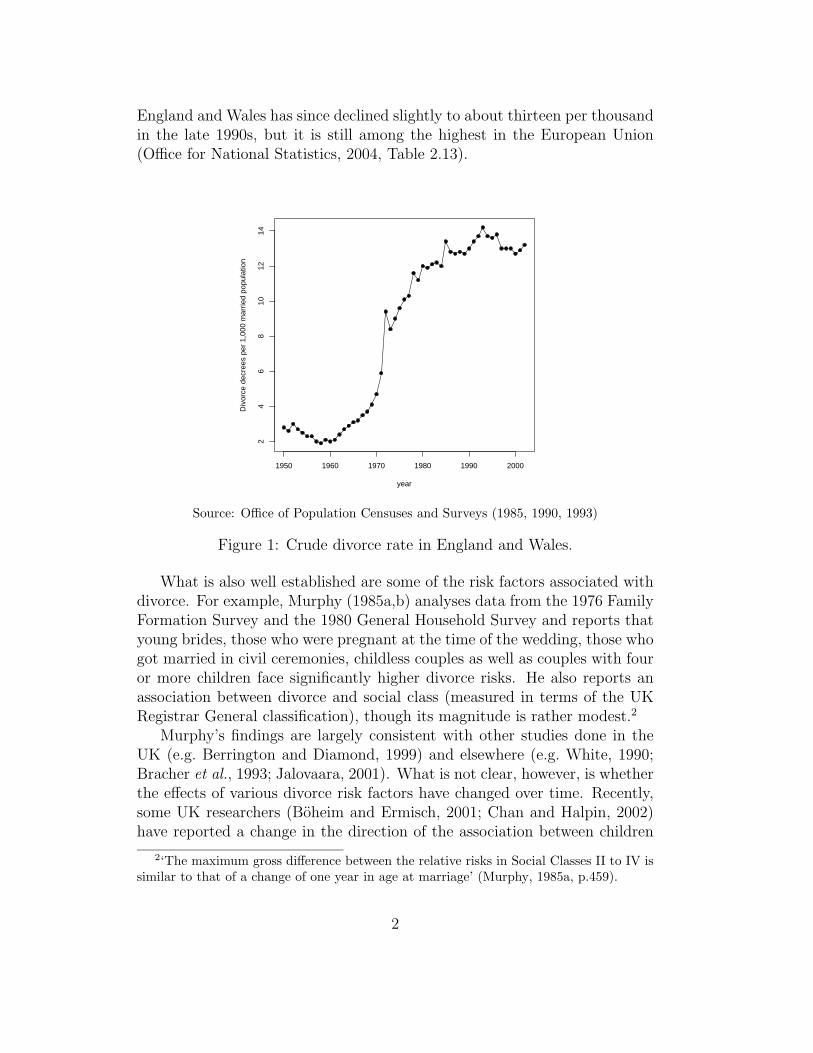
It is well known that the divorce rate in the UK has increased very sharplysince the 1960s. Figure 1 shows the trend for England and Wales, where theannual average between 1950 and 1964 was 2.4 divorces per 1,000 marriages.This increased sixfold to over fourteen divorces per thousand in 1993 (Officeof Population Censuses and Surveys, 1985, 1990, 1993).1 The divorce rate in

∗We thank Yvonne Aberg, Josef Bruderl, Lynn Prince Cooke, Jaap Dronkers, JohnErmisch, John Goldthorpe, Juho Harkonen, Peter Hedstrom, Stephen Jenkins, MatthijsKalmijn, Rob Mare, Mike Murphy, Wendy Sigle-Rushton, Jay Teachman, Michael Wagner,and participants of the third conference of the European Research Network on Divorce inKoln, the GHS User Group, and seminar audiences in Colchester, London, Oxford, Parisand Urbana-Champaign for helpful comments on early drafts.

1The divorce rate of recent years can be found on the web site of the UK Office forNational Statistics: www.statistics.gov.uk.

1

England and Wales has since declined slightly to about thirteen per thousandin the late 1990s, but it is still among the highest in the European Union(Office for National Statistics, 2004, Table 2.13).

1950 1960 1970 1980 1990 2000

24

68

1012

14

year

Div

orce

dec

rees

per

1,0

00 m

arrie

d po

pula

tion

Source: Office of Population Censuses and Surveys (1985, 1990, 1993)

Figure 1: Crude divorce rate in England and Wales.

What is also well established are some of the risk factors associated withdivorce. For example, Murphy (1985a,b) analyses data from the 1976 FamilyFormation Survey and the 1980 General Household Survey and reports thatyoung brides, those who were pregnant at the time of the wedding, those whogot married in civil ceremonies, childless couples as well as couples with fouror more children face significantly higher divorce risks. He also reports anassociation between divorce and social class (measured in terms of the UKRegistrar General classification), though its magnitude is rather modest.2

Murphy’s findings are largely consistent with other studies done in theUK (e.g. Berrington and Diamond, 1999) and elsewhere (e.g. White, 1990;Bracher et al., 1993; Jalovaara, 2001). What is not clear, however, is whetherthe effects of various divorce risk factors have changed over time. Recently,some UK researchers (Boheim and Ermisch, 2001; Chan and Halpin, 2002)have reported a change in the direction of the association between children

2‘The maximum gross difference between the relative risks in Social Classes II to IV issimilar to that of a change of one year in age at marriage’ (Murphy, 1985a, p.459).

2

and marital stability. Using data from the British Household Panel Survey(BHPS), they suggest that in the 1990s British couples with children face sig-nificantly higher divorce risks than similar but childless couples. This is anintriguing and potentially important result as it contradicts established em-pirical findings and widely accepted theories on marital stability (e.g. Beckeret al., 1977).

In this paper we have two objectives. First, we wish to put the unexpectedfinding of Boheim and Ermisch (2001) and Chan and Halpin (2002) to furtherempirical tests using a large and nationally representative data set. And iftheir finding could indeed be confirmed, we shall take some initial steps toexplore why such a change has taken place. Our second goal is to ascertainwhether the effect of other divorce risk factors have changed over time.

2 Stability and change in family formation

and dissolution

It is unusual in the social sciences to see large shifts in the relationship be-tween basic variables, let alone a reversal in the direction of their association.But marriage and the family is one domain in contemporary societies thatis truly in a state of flux. We have seen, for example, large increase in therates of premarital cohabitation and out-of-wedlock birth, the closing of thegender gap in education, and a rise in the employment of married womenwith young children. Many of these factors are well known determinants ofdivorce. But why might their effect be changing?

A possible explanation is that the direct and indirect costs of divorcehave changed. When divorce was relatively expensive, only the rich andresourceful could afford to divorce. But as divorce becomes cheaper, morepeople are able to do so. Such a change would imply a flattening of thedivorce gradient of those variables which index resources, such as income oreducational attainment (Goode, 1993, p.vii). But apart from the changingcosts (and benefits) of divorce, we believe, broadly speaking, two types ofprocesses might be at work. For convenience, we shall refer to them ascomposition effects and contextual effects.

2.1 Composition effects

An example of composition effects concerns premarital cohabitation. It isa well established finding that marriages which began as cohabiting unionsare less stable than those which did not (DeMaris and Rao, 1992; Axinn andThornton, 1992; Lillard et al., 1995). As many researchers have observed,

3

this finding could plausibly be interpreted as arising from a process of self-selection. That is, individuals with non-traditional attitudes about marriageand the family are more likely to cohabit before marriage; but they are alsomore likely to divorce. Thus, the association between premarital cohabitationand marital instability is, under this view, spurious. To the extent that thisis true, because the rate of premarital cohabitation in the UK has risenfrom 3 per cent in the 1960s to over 70 per cent in the 1990s (Berringtonand Diamond, 2000),3 the cohabitants should have become a much less self-selected group, and thus the association between premarital cohabitation andmarital instability should have attenuated over time. However, as the levelof premarital cohabitation gets very high, an opposite self-selection processmight begin to operate: only those who are very conservative about marriageand the family would marry directly. If this group is especially unlikely todivorce, we would expect the association between cohabitation and divorceto become stronger again.

A similar argument could be made in relation to marrying a divorcee.4

When this was very rare, the individuals involved are likely to be a selectedunconventional group. However, as divorce and remarriage become morecommon, this group should become less self-selective. Accordingly, the asso-ciation between remarriage and divorce would attenuate over time.

2.2 Contextual effects

It is also possible that as remarriage becomes more common, the stigmaassociated with them declines, and couples in higher order marriages receivegreater acceptance and support from their friends and relatives, leading to aweakening of the association between remarriage and divorce. But note thatthis argument refers not to a composition effect, but rather to the effect of achanging context, viz. there are more remarriages around.

Along a similar line, Wolfinger (1999) argues that as divorce becomesmore common, children with divorced parents suffer less stigma and traumathan did similar children in the past. Through various psychological andsocial pathways, this might then lead to a reduction of the excess divorcerisks faced by people with divorced parents. Empirically, he shows that inthe US intergenerational transmission rate of divorce risks has declined byalmost 50 per cent between 1973 and 1996.

3See also Figure 3 below. For trends of cohabitation in the US, see Smock (2000) andBumpass and Lu (2000).

4Although the focus of this paper is women in their first marriage, their spouses couldbe divorcees.

4

A further example of contextual effects concerns women’s employment(Becker et al., 1977; Tzeng and Mare, 1995). As South (2001) points out, themarital strain experienced by a working wife might be higher when few mar-ried women work, because under such a condition she is more likely seen asviolating traditional gender role expectations. Furthermore, institutions andpolicies that support women’s employment, such as flexible working sched-ules or childcare facilities, are likely to be less developed. These and otherarguments imply a steeper divorce gradient for women’s employment whenthe overall level of female employment is low. However, South also points outthat the contextual effects might work in the opposite direction. For example,better childcare facilities and flexible schedules might help divorced womencombine paid work and family obligations. The lack of these facilities in anearly period might have made even working wives reluctant to divorce. Asthese facilities develop with rising level of female employment and, further,if working wives are in a better position to take advantage of such facilitiesshould they choose to divorce, the association between women’s employmentand divorce might be stronger when the overall level of female employmentis high. Thus, there is no clear theoretical prediction. Empirically, it is thesecond contextual effect that is supported by his data.

We have noted two mechanisms through which the effect of divorce riskfactors might change. But in evaluating them against empirical results, threepoints should be kept in mind. First, given the nature of the data that isavailable to us, our ability to distinguish between composition and contex-tual effects is rather limited. However, there is one circumstance under whichthe two mechanisms give quite different predictions: as a behaviour or phe-nomenon changes from very rare to very popular, composition effects wouldimply a non-monotonic trend in the relevant parameter (see the discussionon premarital cohabitation above). This is not true for contextual effects.Secondly, it is likely that multiple mechanisms are at work. Thus, if we dofind evidence for composition effects, it does not follow that contextual ef-fects are absent. Thirdly, both composition and contextual effects are drivenby changes in the relative size of different subgroups (e.g. cohabitants andnon-cohabitants) in the population. As we shall see below, there are otherchanges in some divorce predictors which would require more involved expla-nations. We shall discuss these in Section 5.5

5A third class of processes, namely diffusion effects, can also explain shifts in the effectof divorce determinants. For examples of diffusion of demographic behaviour throughsocial networks, see Lesthaeghe and Surkyn (1988), Montgomery and Casterline (1996),Axinn and Yabiku (2001), Kohler et al. (2001), Behrman et al. (2002), and Rindfuss et al.

(2004). However, because of the nature of the data that is available to us, we are not ableto examine this class of processes in this paper.

5

2.3 Empirical research

While there are good reasons to believe that the effect of many divorce riskfactors might be changing, the empirical evidence is far from clear. Teachman(2002) analyses data taken from five rounds of the US National Survey ofFamily Growth. After examining data on first marriages formed between1950 and 1984 with proportional hazard models, he concludes that, with theexception of race, the effects of major sociodemographic predictors have notchanged by historical period.6

However, as noted above, recent research in the UK suggests that theassociation between children and marital stability has changed. Boheim andErmisch (2001) draw their sample from the first eight waves of the BHPS(1991–98). They consider married and cohabiting couples with at least onedependent child in the household. Using discrete time event history models,they show that ‘the risk of partnership dissolution increases with the numberof children’ (Boheim and Ermisch, 2001, p.205).7 Chan and Halpin (2002)use the same BHPS data, but they consider married couples only (with orwithout children). Controlling for a similar set of covariates, they also reportan association between children and higher divorce risks. They then checkthis finding with data collected in the Family and Working Lives Survey(FWLS), a retrospective life-history survey conducted in 1994–95. Using theCox proportional hazard model, but controlling for fewer covariates, theyreport comparable results.

3 Data and methods

Our data come from the General Household Survey (GHS), which is a re-peating general purpose survey conducted by the UK Office for NationalStatistics. The GHS has been running on an annual basis, almost withoutinterruption, since 1971. Each year, about 9,000 households are sampled andface-to-face interviews were conducted with all individuals in these house-holds aged 16 or over. The GHS is a cross-sectional survey, but since 1979respondents were asked quite detailed retrospective questions on marriageand the family. This allows us to reconstruct their complete marriage and

6Teachman (2002) notes that overall blacks have higher divorce rates than whites, butthis gap has been narrowing over time.

7Boheim and Ermisch (2001) control for age at marriage, marriage duration, age of theyoungest child and various characteristics of the respondents and their partners, such asage, religion, ethnicity, educational attainment, employment status, income and financialsurprise.

6

fertility histories. In this paper, we pool together relevant GHS data from1989 to 2000, and focus on women’s first marriage.8

Because of the retrospective nature of the GHS data, almost all of ourcovariates, e.g. year of marriage, age at marriage, premarital cohabitation andeducational attainment, are time-constant in nature. There is just one set oftime-varying covariates, which measures parity.9 We are not able to examinethe dynamic effect of those factors which might themselves be changing overthe course of a marriage, such as women’s employment or family income.

Also, we have only one piece of information about the husbands: whetherthey were previously married.10 Because the GHS is a household survey,there is additional information about the husband of those women who arecurrently married, such as their age or educational attainment. But suchinformation is not available for women whose first marriage had alreadydissolved. This precludes us from including these covariates in the analy-sis. These limitations notwithstanding, the GHS is still an invaluable datasource. It gives us information on the first marriage of 31,381 women who gotmarried between 1960 and 1989. The size of this data set and its temporalcoverage allow us to examine the stability and change of the effect of divorcerisk factors over a period in which family behaviour has been changing mostrapidly.

Table 1 reports the basic descriptive statistics of the covariates. Al-though the overall means and proportions reported in this table are fairlyself-explanatory, we hasten to add that they mask a great deal of changeover time. Thus, for example, while the mean age at marriage of all bridesin our sample is 22.5, there is a well known trend towards late marriage, onewhich has accelerated since the mid-1970s (see Figure 2). Furthermore, thevariation in the age at marriage seems to have increased over time.

A similar point can be made about premarital cohabitation. Overall, 22per cent of all brides in our sample lived with their future husband as acouple before marriage.11 But the level of premarital cohabitation has varied

8Before 1989 information on cohabitation before first marriage was not available for re-spondents who have been married twice or more. Since the multivariate analyses reportedbelow include the covariate of premarital cohabitation, our analysis is based on a smallerdata set of GHS 1989–2000.

9In this paper, we consider children born to the respondents only. There is someinformation on step, adopted and fostered children in the GHS. But the relevant GHSquestions refer to step, adopted and fostered children who are currently living with therespondents. Since step children from dissolved first marriages are probably not livingwith the respondents any more, such information is, for our purpose, incomplete, andtherefore not used in this paper.

10This piece of information is supplied by the respondents.11Because cohabitation with someone other than the respondent’s future husband is not

7

Table 1: Descriptive statistics of covariates.

mean s.d. min. max.

Age at marriage 22.5 4.0 14.5 56.0Number of children 1.9 1.3 0.0 15.0

Premarital birth 7.9%Premarital conception 13.7%Premarital cohabitation 21.9%Husband was a divorcee 8.2%

EducationDegree 18.3%A-level 8.9%O-level 24.6%No qualifications 48.2%

1950 1960 1970 1980 1990 2000

1520

2530

35

year of marriage

age

(yea

rs)

Figure 2: age at marriage of brides (mean, first and thirdquartiles) by year of marriage. Source: pooled GHS data1989–2000.

8

1950 1960 1970 1980 1990 2000

020

4060

80

year of marriage

perc

enta

ge

premarital cohabitation

divorcee

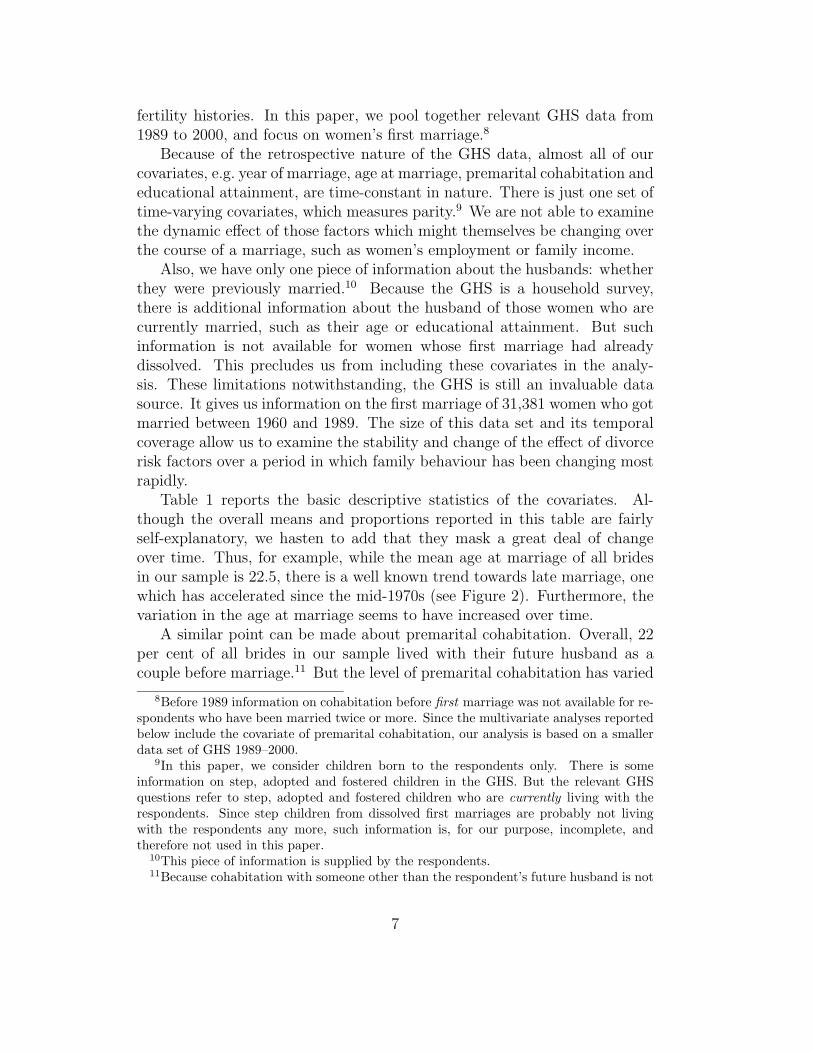
Figure 3: Proportion of brides who cohabited with theirfuture husband before marriage, or married a divorcee byyear of marriage. Source: pooled GHS data 1989–2000.

dramatically across marriage cohorts—from an average of two per cent forthose who married in the 1950s and 1960s to about three quarters in thelate 1990s (see Figure 3). Over the same period, the proportion of womenmarrying a divorcee also rose from three per cent to about 17 per cent.

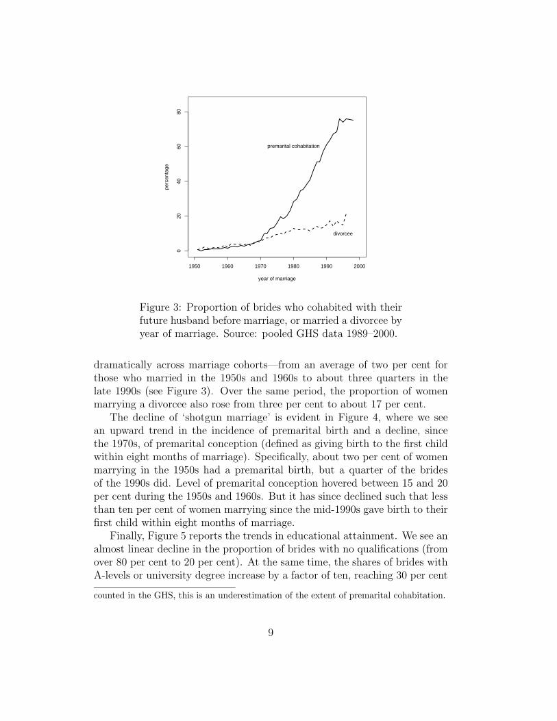
The decline of ‘shotgun marriage’ is evident in Figure 4, where we seean upward trend in the incidence of premarital birth and a decline, sincethe 1970s, of premarital conception (defined as giving birth to the first childwithin eight months of marriage). Specifically, about two per cent of womenmarrying in the 1950s had a premarital birth, but a quarter of the bridesof the 1990s did. Level of premarital conception hovered between 15 and 20per cent during the 1950s and 1960s. But it has since declined such that lessthan ten per cent of women marrying since the mid-1990s gave birth to theirfirst child within eight months of marriage.

Finally, Figure 5 reports the trends in educational attainment. We see analmost linear decline in the proportion of brides with no qualifications (fromover 80 per cent to 20 per cent). At the same time, the shares of brides withA-levels or university degree increase by a factor of ten, reaching 30 per cent

counted in the GHS, this is an underestimation of the extent of premarital cohabitation.

9

1950 1960 1970 1980 1990 2000

05

1015

2025

30

year of marriage

perc

enta

ge

premarital birth

premarital conception

Figure 4: Proportion of brides with premarital birthor premarital conception by year of marriage. Source:pooled GHS data 1989–2000.

and 34 per cent respectively in the late 1990s. These trends are, of course,consistent with what we know about the general expansion of education andthe closing of the gender gap in educational attainment.

4 Results

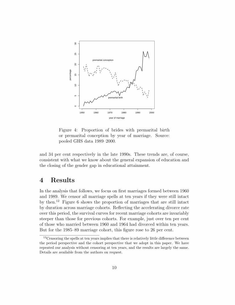
In the analysis that follows, we focus on first marriages formed between 1960and 1989. We censor all marriage spells at ten years if they were still intactby then.12 Figure 6 shows the proportion of marriages that are still intactby duration across marriage cohorts. Reflecting the accelerating divorce rateover this period, the survival curves for recent marriage cohorts are invariablysteeper than those for previous cohorts. For example, just over ten per centof those who married between 1960 and 1964 had divorced within ten years.But for the 1985–89 marriage cohort, this figure rose to 26 per cent.

12Censoring the spells at ten years implies that there is relatively little difference betweenthe period perspective and the cohort perspective that we adopt in this paper. We haverepeated our analysis without censoring at ten years, and the results are largely the same.Details are available from the authors on request.

10

1950 1960 1970 1980 1990 2000

020

4060

80

year of marriage

perc

enta

ge

no qualifications

O−levels

A−levels

degree

Figure 5: Educational attainment of brides by year ofmarriage. Source: pooled GHS data 1989–2000.

months

prop

ortio

n st

ill m

arrie

d

0 24 48 72 96 120

0.7

0.8

0.9

1.0

1960−−641965−−691970−−741975−−791980−−841985−−89

Figure 6: Survival function by marriage cohort.

11

We then fit the Cox proportional hazard model to the data. Our base-line model contains the following covariates: a linear term and a quadraticterm for age at marriage (centred at age 21), year of marriage (centred at1960), and dummies for having one child, two children, three or more children(hereafter as the children dummies), whether the youngest child is less thanfour years old (hereafter as the preschooler parameter), whether the husbandwas a divorcee, premarital cohabitation, and educational attainment (withno qualifications serving as the reference category). This model is fitted toall first marriages in our data, and the parameter estimates are reported inthe first column of Table 2.

It can be seen that, considered over the entire period (i.e. 1960–89),women who marry late face lower divorce risks. For example, comparedto those who married at age 21, the divorce hazard of those marrying at age22 is, on average, 15 per cent lower (1−e−.170+.006). The positive coefficient ofyear of marriage reflects the rising divorce rate over time. Women marryingdivorcees are 29 per cent (e.257

− 1) more likely to divorce, and premaritalcohabitation raises marital instability by 71 per cent (e.539

− 1). The rela-tionship between divorce risks and educational attainment is non-monotonic.Compared with the reference category of women with no qualifications, grad-uates have lower divorce risks, but women with A-levels have higher divorcerisks (though the A-level parameter is marginally insignificant with p = .08).Having a preschooler is associated with substantially lower divorce risks.Controlling for all of the above, the dummies for having one child, two chil-dren, three or more children are all positive, though only the last of theseis statistically significant at the 5% level. These estimates, apart from thoseconcerning children, are not all that exceptional. But are they stable overmarriage cohorts?

To answer this question, we first report in Table 3 the fit statistics of ourbaseline model (model A) and those with an additional term postulating alinear interaction effect between year of marriage and one covariate (or oneset of covariates, see models B to I). On the basis of the likelihood ratio test,it is clear that models B, C, D, E, H and I fit the data better than does thebaseline model, while for model G the improvement in fit is just outside theconventional 5% level. When we allow all covariates to interact with yearof marriage, the fit of model J is again significantly better than that of thebaseline model.13

Thus, in sharp contrast to the US (Teachman, 2002), there is rather

13We would arrive at the same conclusion if BIC is used as the criterion of modelselection, except that models F and G would also be regarded as fitting the data betterthan model A.

12

Table 2: Cox proportional hazard model fitted to episode data of first mar-riage (baseline model).

1960–89 1960–64 1965–69 1970–74 1975–79 1980–84 1985–89

age at marriage -.170** -.198** -.216** -.162** -.166** -.155** -.166**(.006) (.018) (.015) (.013) (.013) (.013) (.014)

age at marr. sq. .006** .022** .012** .007** .006** .005** .005**(.000) (.004) (.002) (.001) (.001) (.001) (.001)

year of marriage .043** .075* .034 .041 -.003 .030 .038(.002) (.032) (.024) (.022) (.021) (.021) (.026)

husband a divorcee .257** .593** .307 .095 .335** .189* .178(.048) (.197) (.171) (.126) (.102) (.094) (.107)

pre. cohabitation .539** 1.014** .786** .660** .423** .467** .524**(.035) (.205) (.138) (.088) (.074) (.064) (.074)

O-levels -.043 -.177 .013 .013 -.088 -.121 .023(.033) (.140) (.090) (.078) (.071) (.070) (.083)

A-levels .091 .724** .070 .019 .095 .039 .037(.051) (.194) (.169) (.125) (.109) (.104) (.117)

university -.097* .011 .281** .101 -.228* -.336** -.272*(.044) (.151) (.104) (.091) (.098) (.103) (.118)

one child .095 -.173 -.395** .100 .065 .174 .499**(.052) (.172) (.130) (.113) (.116) (.116) (.140)

two children .008 -.496** -.435** -.250 -.136 .246 .744**(.058) (.189) (.140) (.130) (.133) (.126) (.149)

three + children .231** -.586* -.289 -.057 .264 .509** 1.018**(.073) (.228) (.176) (.172) (.167) (.157) (.189)

youngest child < 4 -.369** -.016 -.200 -.287** -.462** -.414** -.585**(.045) (.145) (.109) (.099) (.104) (.099) (.124)

# respondents 31381 4669 5796 5903 5182 4888 4943# divorce 5388 478 845 1030 1098 1121 816Log-likelihood -53915.56 -3929.15 -7128.66 -8718.99 -9115.61 -9160.67 -6424.15

Notes: * p < .05, ** p < .01, standard errors in parentheses.

13

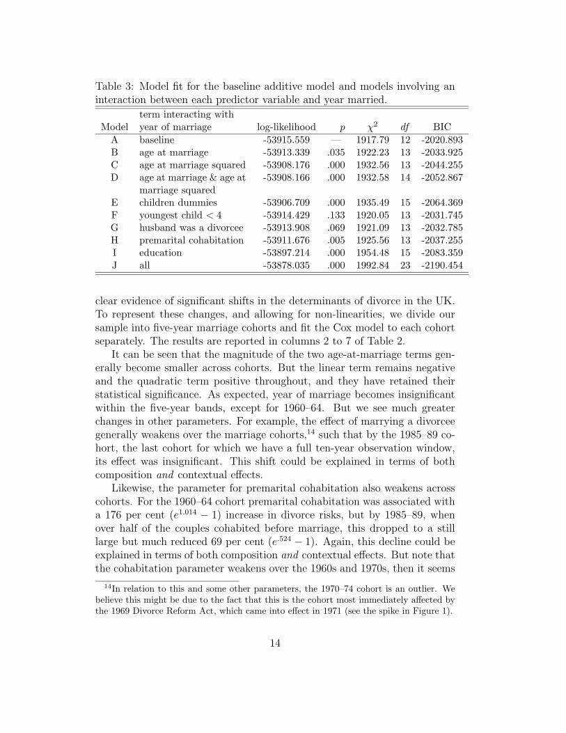
Table 3: Model fit for the baseline additive model and models involving aninteraction between each predictor variable and year married.

term interacting withModel year of marriage log-likelihood p χ2 df BIC

A baseline -53915.559 — 1917.79 12 -2020.893B age at marriage -53913.339 .035 1922.23 13 -2033.925C age at marriage squared -53908.176 .000 1932.56 13 -2044.255D age at marriage & age at

marriage squared-53908.166 .000 1932.58 14 -2052.867

E children dummies -53906.709 .000 1935.49 15 -2064.369F youngest child < 4 -53914.429 .133 1920.05 13 -2031.745G husband was a divorcee -53913.908 .069 1921.09 13 -2032.785H premarital cohabitation -53911.676 .005 1925.56 13 -2037.255I education -53897.214 .000 1954.48 15 -2083.359J all -53878.035 .000 1992.84 23 -2190.454

clear evidence of significant shifts in the determinants of divorce in the UK.To represent these changes, and allowing for non-linearities, we divide oursample into five-year marriage cohorts and fit the Cox model to each cohortseparately. The results are reported in columns 2 to 7 of Table 2.

It can be seen that the magnitude of the two age-at-marriage terms gen-erally become smaller across cohorts. But the linear term remains negativeand the quadratic term positive throughout, and they have retained theirstatistical significance. As expected, year of marriage becomes insignificantwithin the five-year bands, except for 1960–64. But we see much greaterchanges in other parameters. For example, the effect of marrying a divorceegenerally weakens over the marriage cohorts,14 such that by the 1985–89 co-hort, the last cohort for which we have a full ten-year observation window,its effect was insignificant. This shift could be explained in terms of bothcomposition and contextual effects.

Likewise, the parameter for premarital cohabitation also weakens acrosscohorts. For the 1960–64 cohort premarital cohabitation was associated witha 176 per cent (e1.014

− 1) increase in divorce risks, but by 1985–89, whenover half of the couples cohabited before marriage, this dropped to a stilllarge but much reduced 69 per cent (e.524

− 1). Again, this decline could beexplained in terms of both composition and contextual effects. But note thatthe cohabitation parameter weakens over the 1960s and 1970s, then it seems

14In relation to this and some other parameters, the 1970–74 cohort is an outlier. Webelieve this might be due to the fact that this is the cohort most immediately affected bythe 1969 Divorce Reform Act, which came into effect in 1971 (see the spike in Figure 1).

14

to be strengthening again. This non-monotonic pattern is consistent with theview that an opposite selection process begins to operate when cohabitationbecomes very common. This lends support to the view that composition–selection is operating here. But since multiple mechanisms could be at work,one should not rule out the relevance of contextual effects. Furthermore, wenote that the cohabitation parameter is never insignificant. The fact thatcohabitation always has an effect in our model suggests that composition–selection is not the whole story behind the association between premaritalcohabitation and marital instability. It would appear that the cohabitationexperience does have some causal influence on the cohabitants which some-how makes them more prone to divorce.

The changing association with educational attainment is intriguing. Re-call that taken over the entire period of 1960–89, university graduates aresignificantly less likely to divorce than women with no qualifications (see firstcolumn of Table 2). When split into marriage cohorts, the following patternemerges: compared to women with no qualifications, better educated womenused to have higher divorce risks, but the education gradient has now re-versed. For example, in the 1960–64 cohort, women with A-levels were twice(e.724) as likely to divorce as women with no qualifications. But for subse-quent cohorts, the A-levels parameter became statistically insignificant. Asfor university graduates, those who got married in 1965–69 were 32 per cent(e.281

− 1) more likely to divorce than women with no qualifications. Thisparameter became insignificant for the 1970–74 cohort, and then turned neg-ative and significant for subsequent cohorts, such that graduates who marriedbetween 1985 and 1989 were 24 per cent (1−e−.272) less likely to divorce thanwomen with no qualifications.15

4.1 Children and marital stability

Coming to the effect of children, our result is consistent with the finding ofBoheim and Ermisch (2001) and Chan and Halpin (2002). Table 2 showsthat for marriages formed in the 1960s, the children dummies were negativein sign, and four of the six parameters were statistically significant at the 5%level. At the same time, the preschooler parameter was not significant. Thus,it would seem that for these couples, children generally reduced the divorcehazard, and the marriage-stabilising effect of children applied regardless ofthe children’s age.

For marriages formed in the 1970s, the children dummies were insignifi-

15Hoem (1997) reports a similar reversal of the educational gradient in divorce risks forSweden.

15

cant, while the preschooler parameter turned significant. Thus, children werestill associated with marital stability, but only when they were under the ageof four. When we get to the 1985–89 cohort, the children dummies were pos-itive and significant, and their effects were large. Although the preschoolerparameter was also significant and its magnitude had in fact increased, thenet association for having two children, or three or more children, even whenthey were under four, was marriage-destabilising. For example, the divorcerate of those couples with two children (at least one child being a preschooler)was 17 per cent (e.744−.585

−1) higher than otherwise similar but childless cou-ples. Boheim and Ermisch (2001) and Chan and Halpin (2002) use panel datafrom the 1990s to show that children are associated with greater marital in-stability. Using retrospective GHS data, we now see that this shift was wellunderway in the 1980s.

What might account for such a change? It is beyond the scope of this pa-per to address this question in detail. But we shall consider a plausible expla-nation and suggest several reasons as to why it is probably not an importantcontributing factor. The plausible explanation goes as follows. Children areusually a factor protective of marriage because they are a marriage-specificinvestment (Becker et al., 1977). But it has been quite convincingly demon-strated that step children receive less parental investment than biologicalchildren (see e.g. Biblarz and Raftery, 1999; Case et al., 2000). So could thechange in the children parameters be due to the growing prevalence of stepfamilies?

We think not, firstly because in this paper we consider children bornto the respondent only (see note 9). However, we recognise that this doesnot rule out step relationship in the family, as children born to the respon-dent could be step children from the husband’s point of view. We do nothave information on the children’s paternity. But step relationship mightbe thought more likely if the husband was previously married.16 Thus, inanalyses not reported here, we have tested for interaction effects between thechildren parameters and husband’s previous marital status. It turns out thatonly one of the 24 interaction terms (4 × 6 cohorts) are significant at the 5%level. Furthermore, this significant interaction term pertains to the 1965–69cohort, and so cannot explain the change in the 1980s.17

At the end of this section, we shall provide a third argument against the‘step relationship’ or ‘paternity’ interpretation that is based on the timingof cohabiting spell and premarital birth. But at this point, we note that

16For example, the husband could bring his own children from a previous marriage intothe marriage in question, though this is unlikely as custody of children usually goes to themother in the event of divorce.

17Details are available from the authors on request.

16

1960 1965 1970 1975 1980 1985

−1.

0−

0.5

0.0

0.5

1.0

One child

marriage cohort

model 0model 1model 2model 3model 4

1960 1965 1970 1975 1980 1985

−1.

0−

0.5

0.0

0.5

1.0

two children

marriage cohort

model 0model 1model 2model 3model 4

1960 1965 1970 1975 1980 1985

−1.

0−

0.5

0.0

0.5

1.0

Three or more children

marriage cohort

model 0model 1model 2model 3model 4

1960 1965 1970 1975 1980 1985

−1.

0−

0.5

0.0

0.5

1.0

Youngest child < 4

marriage cohort

model 0model 1model 2model 3model 4

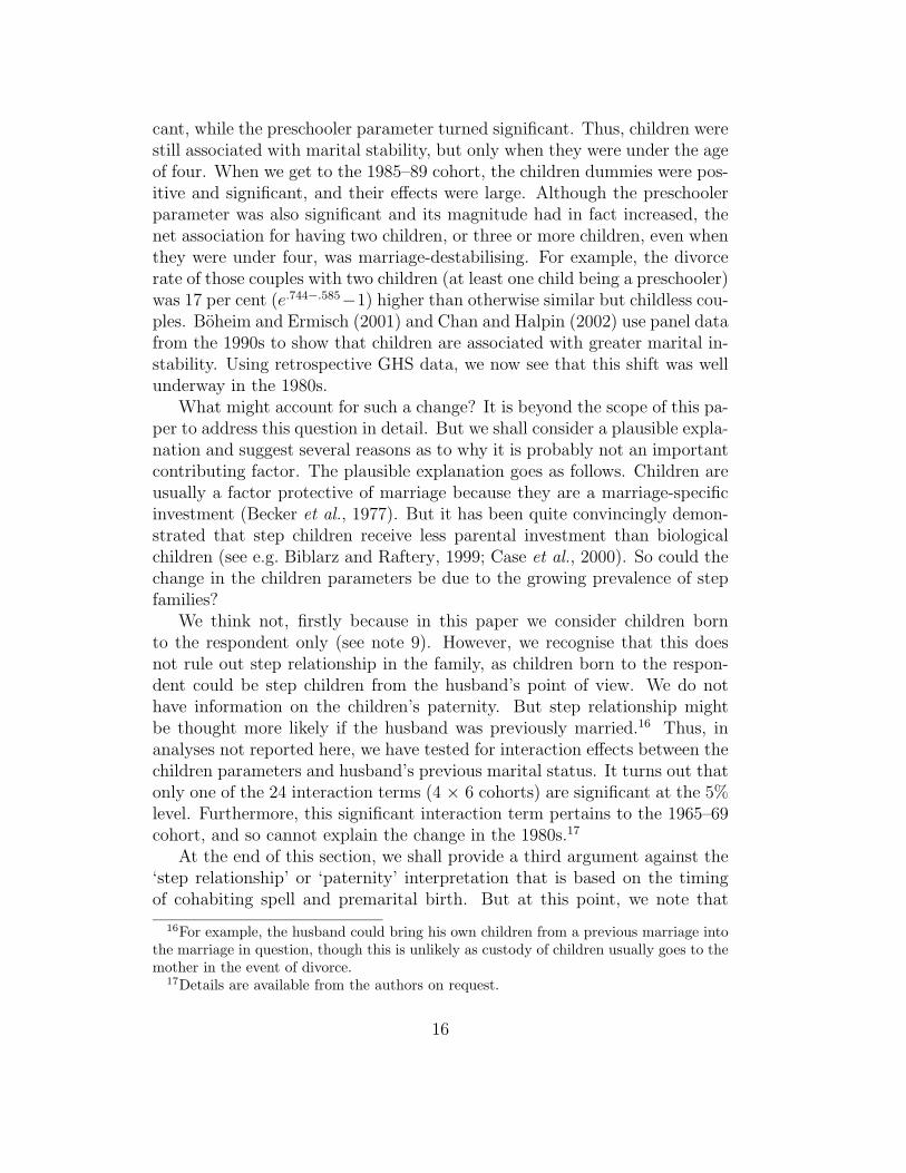
Figure 7: Estimated effects of the children dummies and the preschoolerparameter under different models.Note: Model 0 contains the three children dummies and the preschooler parameter only.

Model 1 is the baseline model reported in columns 2 to 7 of Table 2. Model 2 is the

baseline model plus a dummy for premarital conception. Model 3 is the baseline model

plus dummies for premarital conception and premarital birth (see Table 4). Model 4

substitutes the premarital birth parameter of model 3 with three separate dummies

indicating whether premarital birth took place without cohabitation, before cohabitation

or during a cohabiting spell (see Table 5). “•” denotes that the parameter estimate is

significantly different from zero at the 5% level, while “+” denotes that it is not.17

previous research suggests that the association between children and maritalstability is multidimensional. Not only are the number of children and theirage important, the timing of childbirth also matters (e.g. Murphy, 1985a;Waite and Lillard, 1991). To disentangle the effect of timing from thoseof number and age, we control for premarital conception and premaritalbirth in the model. Figure 7 shows how the inclusion of these terms affectsthe children dummies and the preschooler parameter. Model 0 is the nullmodel in the sense that it contains the children parameters only. Thus, theparameter estimates of the null model show the gross association betweenchildren and marital stability. Model 1 is the baseline model reported incolumns 2 to 7 of Table 2. In both models 0 and 1 the children dummiesgenerally trend upward, while the preschooler parameter trends downward.As we saw in Table 2, for those who got married in the late 1980s, havingchildren is associated with significantly higher divorce risks.

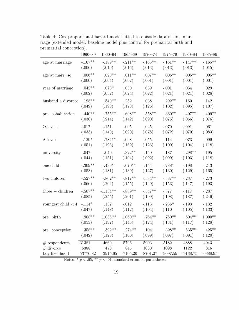
When we control for premarital conception in model 2, the children dum-mies and the preschooler parameter change little, as can be seen from theclose proximity of the lines for models 1 and 2 in Figure 7. However, when wefurther control for premarital birth in model 3, the estimates for the childrendummies remained negative throughout, although they became insignificantfor the last two cohorts. The preschooler parameter also becomes insignifi-cant once premarital birth is taken into account. Thus, it would seem thatthe destabilising effect of children is related to the growth of premarital birthin recent years. But it should be noted that even under model 3 the generaltrend is for the children dummies to become less negative (i.e. less stabilis-ing). We report the parameter estimates of model 3 in Table 4. (Figure 7also contains a Model 4 which we shall discuss below.)

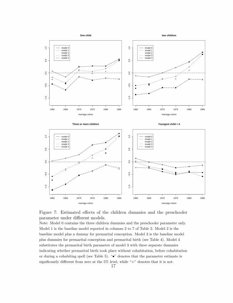
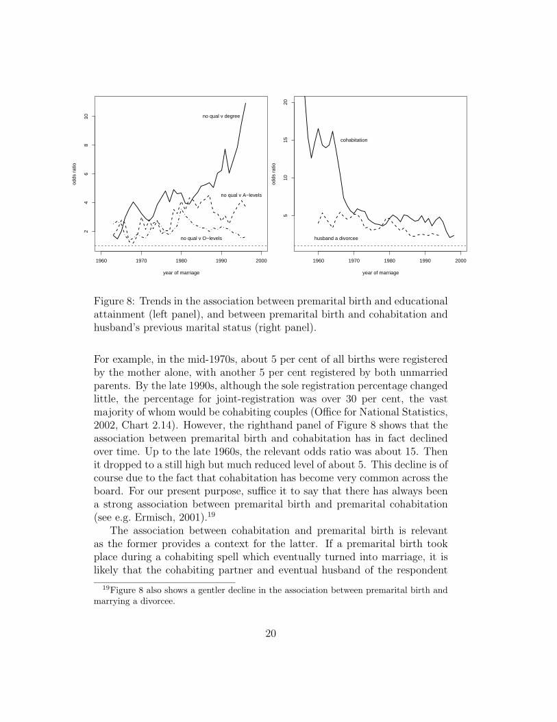
Given the apparent importance of premarital birth, two questions comenaturally to mind. First, who are more likely to have premarital birth?Secondly, under what circumstances is premarital birth especially likely toaccentuate the association between children and marital instability? To an-swer the first of these questions, the lefthand panel of Figure 8 shows theassociation between educational attainment and premarital birth. It is strik-ing how that association has strengthened over time. For example, in the1960s, the odds of a woman with no qualifications having a premarital birthwas about 2 to 3 times that of a female graduate. By the late 1980s, theodds ratio has risen to almost 6, which gets even higher in the 1990s.18

As regards the second question, we note that childbirth timing is relatedto other social changes discussed above, especially premarital cohabitation.

18We have carried out some data smoothing for Figure 8 by averaging the contingencytable of any year with those of the immediately preceding and subsequent years.

18

Table 4: Cox proportional hazard model fitted to episode data of first mar-riage (extended model: baseline model plus control for premarital birth andpremarital conception).

1960–89 1960–64 1965–69 1970–74 1975–79 1980–84 1985–89

age at marriage -.167** -.189** -.211** -.165** -.161** -.147** -.165**(.006) (.019) (.016) (.013) (.013) (.013) (.015)

age at marr. sq. .006** .020** .011** .007** .006** .005** .005**(.000) (.004) (.002) (.001) (.001) (.001) (.001)

year of marriage .042** .073* .030 .039 -.001 .034 .029(.002) (.032) (.024) (.022) (.021) (.021) (.026)

husband a divorcee .198** .540** .252 .038 .292** .160 .142(.049) (.198) (.173) (.126) (.102) (.095) (.107)

pre. cohabitation .440** .755** .608** .558** .360** .407** .409**(.036) (.214) (.142) (.090) (.075) (.066) (.076)

O-levels -.017 -.151 .005 .025 -.070 -.091 .061(.033) (.140) (.090) (.078) (.072) (.070) (.083)

A-levels .129* .784** .098 .055 .114 .073 .099(.051) (.195) (.169) (.126) (.109) (.104) (.118)

university -.047 .040 .322** .140 -.187 -.298** -.195(.044) (.151) (.104) (.092) (.099) (.103) (.118)

one child -.309** -.439* -.670** -.154 -.288* -.198 -.243(.058) (.181) (.139) (.127) (.130) (.129) (.165)

two children -.527** -.862** -.817** -.584** -.587** -.237 -.273(.066) (.204) (.155) (.149) (.153) (.147) (.193)

three + children -.507** -1.134** -.889** -.547** -.377 -.117 -.287(.085) (.255) (.201) (.199) (.198) (.187) (.246)

youngest child < 4 -.114* .137 -.012 -.115 -.236* -.193 -.132(.047) (.148) (.112) (.104) (.110 (.105) (.133)

pre. birth .908** 1.035** 1.060** .764** .750** .604** 1.090**(.053) (.197) (.145) (.124) (.131) (.117) (.128)

pre. conception .358** .392** .274** .104 .398** .535** .425**(.042) (.128) (.100) (.099) (.097) (.091) (.120)

# respondents 31381 4669 5796 5903 5182 4888 4943# divorce 5388 478 845 1030 1098 1122 816Log-likelihood -53776.82 -3915.65 -7105.20 -8701.27 -9097.59 -9138.75 -6388.95

Notes: * p < .05, ** p < .01, standard errors in parentheses.

19

1960 1970 1980 1990 2000

24

68

10

year of marriage

odds

rat

io

no qual v degree

no qual v A−levels

no qual v O−levels

1960 1970 1980 1990 2000

510

1520

year of marriageod

ds r

atio

cohabitation

husband a divorcee

Figure 8: Trends in the association between premarital birth and educationalattainment (left panel), and between premarital birth and cohabitation andhusband’s previous marital status (right panel).

For example, in the mid-1970s, about 5 per cent of all births were registeredby the mother alone, with another 5 per cent registered by both unmarriedparents. By the late 1990s, although the sole registration percentage changedlittle, the percentage for joint-registration was over 30 per cent, the vastmajority of whom would be cohabiting couples (Office for National Statistics,2002, Chart 2.14). However, the righthand panel of Figure 8 shows that theassociation between premarital birth and cohabitation has in fact declinedover time. Up to the late 1960s, the relevant odds ratio was about 15. Thenit dropped to a still high but much reduced level of about 5. This decline is ofcourse due to the fact that cohabitation has become very common across theboard. For our present purpose, suffice it to say that there has always beena strong association between premarital birth and premarital cohabitation(see e.g. Ermisch, 2001).19

The association between cohabitation and premarital birth is relevantas the former provides a context for the latter. If a premarital birth tookplace during a cohabiting spell which eventually turned into marriage, it islikely that the cohabiting partner and eventual husband of the respondent

19Figure 8 also shows a gentler decline in the association between premarital birth andmarrying a divorcee.

20

is the father of the child. One might argue that premarital births of thistype are comparable to marital births. But for premarital births which tookplace before the cohabiting spell or without cohabitation, there is a higherprobability that it was someone else who fathered the child.20 In a sense,this argument goes back to the question of step-relationship and paternity.To test this idea, we distinguish three types of premarital birth: those whichtook place (1) without cohabitation, (2) before cohabitation, and (3) duringcohabitation. We replace the premarital birth dummy of Table 4 with thesethree dummies and repeat the analysis. The relevant results are reported inTable 5.21

Table 5: Cox proportional hazard model fitted to episode data of first mar-riage (modified extended model: premarital birth dummy replaced by threedummies indicating the timing of premarital birth relative to premarital co-habitation).

1960–89 1960–64 1965–69 1970–74 1975–79 1980–84 1985–89

Pre. birth without 1.056** 1.113** 1.123** .879** 1.051** .856** 1.434**cohabitation (.066) (.208) (.154) (.141) (.149) (.168) (.182)

Pre. birth before .813** .488 1.162** .497* .421 .583** .959**cohabitation (.089) (.489) (.367) (.245) (.258) (.171) (.170)

Pre. birth during .709** 1.032 .513 .590* .231 .385* .958**cohabitation (.086) (.561) (.395) (.238) (.246) (.171) (.153)

Note: * p < .05, ** p < .01, standard errors in parentheses. Other parameters of the

model, such as age at marriage, education, children dummies or premarital cohabitation

are not shown, but are available from the authors on request.

As readers can see, there is partial support for the above argument. Whilethe parameters for type 1 premarital birth are always positive and signifi-cant, those for type 2 and type 3 premarital birth are significant in four andthree marriage cohorts respectively. Furthermore, where a type 3 parame-ter is significant, its magnitude tends to be considerably smaller than thecorresponding type 1 parameter (i.e. premarital birth without cohabitation),though the pattern is less clear when we compare the magnitude of type 2 and

20We thank Josef Bruderl for this thoughtful suggestion.21The model in Table 5 also contains all the other parameters considered above. But

since they are substantively very similar to those of Table 4, we do not report them here.Details are available from the authors on request.

21

type 3 premarital births.22 Having said that, we note that all three typesof premarital birth are significant in the last two marriage cohorts. Moreimportantly, the children dummies and the preschooler parameter are unaf-fected when the distinction of three types of premarital birth is introduced.If we go back to Figure 7, it can be seen that the lines for model 3 (where weuse one parameter for all premarital births) and model 4 (three parameters)are virtually indistinguishable from each other. This result reinforces ourview that paternity or step-relationship is not a key factor which led to theobserved change in the association between children and marital stability.

5 Summary and discussion

In this paper, we use retrospective marriage history data to show that inthe UK the effects of many predictors of divorce have changed over time.In contrast to Teachman (2002), who finds a pattern of overall stability inthe US, we find substantial, systematic and quite interpretable change inthe effects of education, premarital cohabitation, marriage to a divorcee, andchildren.

As the rate of premarital cohabitation rose from less than 5 per cent inthe 1960s to about 50 per cent in the 1980s, the coefficient of our cohabi-tation parameter almost halves in magnitude (.409/.755, see Table 4). Theestimate for marrying a divorcee also weakens over time, such that it becameinsignificant for the 1985–89 marriage cohort. The change of these two pa-rameters could, at least in part, be explained in terms of composition effects,i.e. as cohabitation and remarriage become more common, they become lessselective and tell us less about the individuals involved. But it is also possi-ble that as cohabitation and remarriage become more common, they becomesocially more acceptable, leading to a weakening of their association withmarital instability (i.e. contextual effects).

We have noted one unique implication of composition effects: that is,as previously rare behaviour becomes very popular, there would be selectionfrom the opposite direction, leading to a non-monotonic trend in the relevantparameter. This seems to be the case for premarital cohabitation, thoughwe need data from even more recent marriage cohorts to confirm our initial

22Compared with marriage, cohabitation is a less well-defined state (Murphy, 2000), andthere would be a higher degree of measurement error in the reporting of the beginningdate of cohabitation spells. Note that this is not just a matter of recall error. For manycohabitants, there is a gradual process from staying over occasionally to finally movingin. Such measurement errors mean that the distinction between premarital births whichhappened before and those which happened during a cohabitation spell is not very clearcut.

22

finding. Moreover, as we have noted above, the fact that composition effectsare at work does not imply that other mechanisms are irrelevant. It is morethan likely that multiple mechanisms are operating.

Among women who got married in the 1960s, it was the better educatedwho faced higher divorce risks. Over time, the education gradient has notonly flattened but reversed, such that for those who got married in the 1980s,university graduates were less likely to divorce than women with no quali-fications. A flattening of the education gradient could be explained by thedeclining costs of divorce or some composition–selection process.23 But areversal of the gradient suggests that additional factors are involved. With-out further investigation, we could only offer some speculative remarks here.First, it could be the case that with greater female access to the labourmarket, and pressure (from the housing market and elsewhere) to have twoincomes, British society has become more accepting of educated and econom-ically successful women.

Thirdly, it is also possible that the expansion of higher education andthe closing of the gender gap in educational attainment have made univer-sities and colleges more efficient institutions for sorting and matching po-tential spouses. Whether this happened, and if so how, are questions forfuture investigation. Halpin and Chan (2003) recently report that both ab-solute and relative rates of educational assortative mating has declined inthe UK between 1973 and 1995. But we note that the measures used inthat paper (e.g. percentage of cases off the main diagonal in a square ta-ble cross-classifying husband’s and wife’s education, and uniform differenceparameters) are global measures. That is, they pertain to all levels of ed-ucational attainment. More work on assortative mating that is sensitiveto the experience of people with specific levels of education would be veryilluminating.

The effect of children has been one of our main concerns. Previous re-search has demonstrated a reversal of the familiar protective effect of chil-dren on marriages, and we replicate that result here with a different data set.We have offered several arguments to suggest that the destabilising effect ofchildren in recent cohorts is not due to the growing prevalence of step rela-tionship. We then demonstrate that the change is related to the growth ofpremarital birth. Premarital birth, we further show, is becoming ever morestrongly associated with low educational attainment.

23When very few women were going to university, they would be a very selected uncon-ventional group. Perhaps many of them were especially independent and focussed on theircareer, which might explain the higher divorce risks they faced. When more women aregoing to universities, such composition effects should become weaker, and the educationgradient flatter.

23

The last observation is important because, as we have shown, the lessqualified have recently become more likely to divorce than graduates anyway.But they are also much more likely to have premarital births (see Figure 8),which means that their children are likely to have a marriage-destabilising

effect. Thus, children born to mothers with no qualifications are much morelikely to go through a parental divorce and suffer its consequences. Com-pounding this is the link between low wage and no qualifications. Overall, thewelfare implications for individuals, especially the children, is considerable.Our results clearly echo some of the concerns for the ‘diverging destinies’ ofUS children expressed recently by McLanahan (2004).

The importance of premarital birth in the change of the children effectspeaks obviously to the platitude that we need to know the process of familyformation before we can understand the process of family dissolution. Butpremarital birth is probably not the complete explanation for the observedchange. As we point out in relation to model 3 in Figure 7, even whenpremarital birth is taken in account, the overall trend is for the children effectto become less stabilising over time. This raises the question of whether inthe UK the overall level of parental investment in children has been decliningas well as polarising. We intend to pursue this important question with UKsurvey data on family expenditure and time use (cf. Sayer et al., 2004).

References

Axinn, W. G. and Thornton, A. (1992). The relationship between cohabi-tation and divorce: Selectivity or causal influence? Demography, 29(3),357–374.

Axinn, W. G. and Yabiku, S. T. (2001). Social change, the social organizationof families, and fertility limitation. American Journal of Sociology, 106(5),1219–1261.

Becker, G. S., Landes, E. M., and Michael, R. T. (1977). An economicanalysis of marital instability. Journal of Political Economy, 85(6), 1141–1187.

Behrman, J. R., Kohler, H.-P., and Watkins, S. C. (2002). Social networksand change in contraceptive use over time: Evidence from a longitudinalstudy in rural Kenya. Demography, 39(4), 713–738.

Berrington, A. and Diamond, I. (1999). Marital dissolution among the 1958British birth cohort: The role of cohabitation. Population Studies, 53(1),19–38.

24

Berrington, A. and Diamond, I. (2000). Marriage or cohabitation: A com-peting risks analysis of first-partnership formation among the 1958 Britishbirth cohort. Journal of the Royal Statistical Society, Series A, 163(2),127–151.

Biblarz, T. J. and Raftery, A. E. (1999). Family structure, educational at-tainment, and socioeconomic success: Rethinking the “pathology of ma-triarchy”. American Journal of Sociology, 105(2), 321–365.

Boheim, R. and Ermisch, J. (2001). Partnership dissolution in the UK —the role of economic circumstances. Oxford Bulletin of Economics and

Statistics, 63(2), 197–208.

Bracher, M., Santow, G., Morgan, S. P., and Trussell, J. (1993). Marriagedissolution in Australia. Population Studies, 47, 403–425.

Bumpass, L. and Lu, H.-H. (2000). Trends in cohabitation and implicationsfor children’s family contexts in the united states. Population Studies, 54,29–41.

Case, A., Lin, I., and McLanahan, S. (2000). How hungry is the selfish gene?The Economic Journal, 110, 781–804.

Chan, T. W. and Halpin, B. (2002). Union disruption in the United Kingdom.International Journal of Sociology, 32(4), 76–93.

DeMaris, A. and Rao, K. V. (1992). Premarital cohabitation and subsequentmarital stability in the United States: A reassessment. Journal of Marriage

and the Family, 54, 178–190.

Ermisch, J. (2001). Cohabitation and childbearing outside marriage inBritain. In L. L. Wu and B. Wolfe, editors, Out of Wedlock: Causes and

Consequences of Nonmarital Fertility, chapter 4, pages 109–139. RussellSage Foundation, New York.

Goode, W. J. (1993). World Changes in Divorce Patterns. Yale UniversityPress, New Haven.

Halpin, B. and Chan, T. W. (2003). Educational homogamy in Ireland andBritain: Trends and patterns. British Journal of Sociology, 54(4), 473–495.

Hoem, J. M. (1997). Educational gradients in divorce risks in Sweden inrecent decades. Population Studies, 51, 19–27.

25

Jalovaara, M. (2001). Socio-economic status and divorce in first marriagesin Finland 1991–93. Population Studies, 55, 119–133.

Kohler, H.-P., Behrman, J. R., and Watkins, S. C. (2001). The densityof social networks and fertility decisions: Evidence from south Nyanzadistrict, Kenya. Demography, 38(1), 43–58.

Lesthaeghe, R. and Surkyn, J. (1988). Cultural dynamics and economictheories of fertility change. Population and Development Review, 14(1),1–45.

Lillard, L. A., Brien, M. J., and Waite, L. J. (1995). Premarital cohabitationand subsequent marital dissolution: A matter of self-selection? Demogra-

phy, 32(3), 437–457.

McLanahan, S. (2004). Diverging destinies: how children are faring underthe second demographic transition. Demography, 41(4), 607–627.

Montgomery, M. R. and Casterline, J. B. (1996). Social learning, socialinfluence, and new models of fertility. Population and Development Review,22(1), 151–175.

Murphy, M. (2000). Editoral: Cohabitation in Britain. Journal of the Royal

Statistical Society, Series A, 163(2), 123–126.

Murphy, M. J. (1985a). Demographic and socio-economic influences on recentbritish marital breakdown patterns. Population Studies, 39, 441–460.

Murphy, M. J. (1985b). Marital breakdown and socio-economic status: Areappraisal of the evidence from recent british sources. British Journal of

Sociology, 36(1), 81–93.

Office for National Statistics (2002). Social Trends, volume 32. HMSO,London.

Office for National Statistics (2004). Social Trends, volume 34. HMSO,London.

Office of Population Censuses and Surveys (1985). Marriage and Divorce

Statistics: Review of the Registrar General on Marriages and Divorces in

England and Wales, 1982. Number 19 in Series FM2. HMSO, London.

Office of Population Censuses and Surveys (1990). Marriage and Divorce

Statistics: Historical Series of Statistics on Marriages and Divorces in

England and Wales, 1837–1983. Number 16 in Series FM2. HMSO, Lon-don.

26

Office of Population Censuses and Surveys (1993). Marriage and Divorce

Statistics: Review of the Registrar General on Marriages and Divorces in

England and Wales, 1993. Number 19 in Series FM2. HMSO, London.

Rindfuss, R. R., Choe, M. K., Bumpass, L. L., and Tsuya, N. O. (2004).Social networks and family change in Japan. American Sociological Review,69(6), 838–861.

Sayer, L. C., Bianchi, S. M., and Robinson, J. P. (2004). Are parents invest-ing less in children? trends in mothers’ and fathers’ time with children.American Journal of Sociology, 110(1), 1–43.

Smock, P. J. (2000). Cohabitation in the United States: An appraisal ofresearch themes, findings, and implications. Annual Review of Sociology,26, 1–20.

South, S. J. (2001). Time-dependent effects of wives’ employment on maritaldissolution. American Sociological Review, 66(2), 226–245.

Teachman, J. D. (2002). Stability across cohorts in divorce risk factors.Demography, 39(2), 331–351.

Tzeng, J. M. and Mare, R. D. (1995). Labor market and socioeconomiceffects on marital stability. Social Science Research, 24, 329–351.

Waite, L. J. and Lillard, L. A. (1991). Children and marital disruption.American Journal of Sociology, 96(4), 930–953.

White, L. K. (1990). Determinants of divorce: A review of research in theeighties. Journal of Marriage and the Family, 52(4), 904–912.

Wolfinger, N. H. (1999). Trends in the intergenerational transmission ofdivorce. Demography, 36(3), 415–420.

27