Soft Information And The Cost Of Job Rotation:

Evidence From Loan Officer Rotation∗

Subhendu Bhowal Krishnamurthy Subramanian

Prasanna Tantri

July 2014

We highlight the costs from a principal rotating agents among tasks when decision-

making inside a firm is driven by soft information. These costs arise because (i) an

incoming agent cannot verify the information set that the outgoing agent utilised, and

(ii) neither agent receives the entire marginal benefit/penalty for her effort. We provide

evidence of this cost using unique loan and officer level data from a large public sector

bank in India. Using the bank’s fixed-tenure-based policy of loan officer rotation for

identification, we find that default probabilities are 7.5% higher for loans affected by job

rotation when compared to other loans. This difference is not explained by differences in

hard information or the loss of a lending relationship.

Key Words : Agency Costs, Bank, Default, Hard Information, Loan, Rotation, Soft In-

formation, Relationship Banking.

JEL Classification: C72, G20, G21, G28, G30, G38, L51, M52.

Please address correspondence to:

Krishnamurthy Subramanian, Indian School of Business, Gachibowli, Hyderabad, 500032,

India. Email: Krishnamurthy Subramanian@isb.edu

∗All authors are from the Indian School of Business, Hyderabad, India. We would like to thankManju Puri for her detailed comments as part of the review provided under the aegis of the NationalStock Exchange (NSE) - New York University (NYU) grant. We also thank for their comments andsuggestions Rajesh Chakrabarti, Subir Gokarn, Atif Mian, Nachiket Mor, Rajkamal Iyer and seminarand conference participants at the Multinational Finance Society Symposium, Cyprus. We would alsolike to thank Center for Analytical Finance, Indian School of Business for providing the data and otherassistance for this project. This research is supported by the National Stock Exchange (NSE) - NewYork University (NYU) grant. The usual disclaimer applies.

I Introduction

This paper examines the policy of rotating agents between tasks in order to miti-

gate agency problems in communication within an organization. Few empirical studies

have examined the implications of a well defined rotation policy. A notable exception

is Hertzberg, Liberti, and Paravisini (2010), who study loan officer rotation in a bank

and find that rotation policy creates incentives for the outgoing agent to reveal private

information truthfully towards the end of her tenure, which leads to more efficient capital

allocation. However, the possible costs associated with a rotation policy have not received

attention in the empirical literature. In this paper, we argue that rotation policies can be

costly when soft information dominates decision-making inside a firm. The cost we high-

light stems from the inability to verify soft information. We provide evidence supporting

our thesis using unique data for bank loans and the loan officers that make these loans.

We find that mandatory rotation of loan officers leads to outgoing loan officers making

lower effort when the officer’s tenure in a bank branch is expected to come to an end.

Such distortion in loan officer incentives, in turn, leads to inefficient capital allocation by

the bank.

Delegation of tasks to agents is a reality in all organizations. While delegation induces

the agent to maximize effort, it also leads to loss of control for the principal (Aghion and

Tirole (1997); Stein (2003)). Delegating authority to an agent can also create other

problems such as collusion, sub-optimal performance, etc. These problems stem from

the fact that the agent, in her normal course of business, acquires private information

that the principal has no access to. Moreover, the congruence between the interests of a

principal and an agent vary with the nature of the task and the circumstances in which

the task is carried out. Rotation of agents among tasks has been suggested as a solution

for eliciting private information from agents (Arya and Mittendorf, 2004).

We argue that job rotation imposes costs when decision-making inside the firm is

driven by soft information because (i) an incoming agent cannot verify the information

set that the outgoing agent utilised, and (ii) neither agent receives the entire marginal

benefit/penalty for her effort. We study this cost of job rotation inside a bank for the fol-

lowing reasons. First, because bank lending relies on relationships and soft information,1

decision-making inside the bank provides an ideal setting to study this cost. Second,

ex-post default on a loan represents a concrete and verifiable outcome measure that, in

turn, depends upon unverifiable sets of information. Such an empirical setup is rarely

available in other organizational settings.

In a bank, a rotation policy creates a peculiar situation with respect to loans lent

during the end of a loan officer’s tenure. By design, the outgoing and incoming officers

1See Ramakrishnan and Thakor (1984); Rajan (1992); Petersen and Rajan (1995); Petersen andRajan (2002); Stein (2002); Petersen (2004); Berger, Miller, Petersen, Rajan, and Stein (2005).

1

become responsible for the performance of such a loan. While the outgoing loan officer

is responsible for screening and due diligence at the time of lending, the incoming officer

bears responsibility for monitoring and collecting the dues. Thus, job rotation transforms

a simple incentive problem, where employee performance can be possibly rewarded based

on how the loan performs, into a problem of moral hazard in teams (Holmstrom (1982)).

If the efforts made by the incoming and outgoing officers are verifiable, then the firm can

create incentive structures where each employee reaps the benefit/penalty proportional

to his (measurable) contribution. Moreover, as Hertzberg, Liberti, and Paravisini (2010)

highlight, if effort is verifiable then job rotation creates the possibility that the outgoing

officer reveals his predecessor’s effort. As a result, career concerns motivate the predeces-

sor to provide effort optimally. However, when the information collected by the employee

is soft, neither the information nor the effort at collecting the same can be verified. In

this case, as in Holmstrom and Milgrom (1991), the number of observables—default on

the loan in this case—is less than the number of activities performed by two different

agents. Therefore, the firm cannot design an incentive contract that rewards each em-

ployee partially according to this effort. Using a simple theoretical model presented in

Section IV, we show that a rotation policy therefore leads to an equilibrium where both

the officers exert low effort for loans lent at the end of the outgoing loan officer’s tenure.

This result is obtained due to the combination of two factors. First, due to the problem

of moral hazard in teams, neither officer receives in toto the marginal benefit from (or

penalty for) her effort. Second, when lending is based on soft information, the incoming

loan officer finds it hard to verify the level of effort exerted by the outgoing officer in

screening the loan. Similarly, the outgoing officer cannot verifiably prove to his superiors

that the incoming loan officer may have exerted low effort in monitoring the loan and

collecting the dues. Our second assumption is based on the fact that decision-making

inside banks is dominated by soft information. This assumption is motivated not only by

bank lending relying on soft information in general (Petersen (2004); Ramakrishnan and

Thakor (1984)) but also by the findings in Fisman, Paravisini, and Vig (2012). They show

in the Indian context that informal relationships between a loan officer and a borrower

play a major role in lending and repayment decisions.

We test our hypothesis using unique data for bank loans and the loan officers that

make these loans. This data was provided to us by a large public sector bank in India.

Apart from internal audits, audit by the officials from the Reserve Bank of India ensures

that our data are authentic. Even though the loan account data provided to us span the

time period October 2005 to May 2012, we restrict our analysis to loans issued till May

2011. The agricultural crop loans that we employ for our analysis have a maturity of

one year. Therefore, restricting our analysis to loans issued till May 2011 ensures that

we have data on loan performance for all the loans in our sample. The data comprise

of 45592 agricultural crop loans issued by 51 loan officers over the time period October

2

2005 to May 2011; of these 45592 loans, 25976 loans constitute repeat loans.

To identify the effect of job rotation on loan performance, as in Hertzberg, Liberti,

and Paravisini (2010) and Fisman, Paravisini, and Vig (2012), we exploit the mandatory

rotation policy employed at the bank. As part of this policy, the bank rotates its loan

officers once the officer has completed three years in a particular branch. Typically,

rotation of loan officers in a bank may be correlated with their prior performance, which

would spoil identification. However, public sector banks in India are bureaucratic and

operate based on rigid rules. As well, the employees of public sector banks in India are

heavily unionised and oppose any rotation that deviates from the set rules.2 Thus, in

our setting, rotation of loan officers occurs based on a rule rather than as a reaction to

loan officer performance. Though de jure loan officers should get rotated exactly after

completing three years, de facto loan officer tenure exhibits some variation around three

years. This variation comes about because a loan officer has to wait for a replacement

to be identified and for the replacement to take over responsibilities from him, which

leads to many loan officers’ tenure being more than three years. On the other side of

the spectrum, we inferred through our interviews with the bank officials and our review

of official documents that administrative exigencies contribute to tenure of some loan

officers being less than three years. Figure 2 shows how the likelihood of a loan officer

remaining in her current job varies with her tenure. We observe a sharp discontinuity at

three years, which illustrates that the bank’s rotation policy of transferring officers after

three years indeed operates on the ground.

We use the sample of agricultural crop loans made by the bank. Agricultural crop

loans provide us two key advantages. First, as we argue in Section III.A, agricultural

lending in a developing country like India is based primarily on soft information. Second,

because agricultural crop loans have a fixed maturity of one year, we can cleanly separate

loan officers into “treatment” and “control” groups to estimate the effect of a rotation

policy. Because the expected tenure equals three years, an officer that has completed two-

and-a-half years in office is more likely to make a loan that would straddle her tenure and

that of her replacement. These officers represent our “treatment” group. In contrast,

a loan officer that has not completed two-and-a-half years in office is less likely to be

involved in such a loan. As in Hertzberg, Liberti, and Paravisini (2010), these officers

represent our “control” group. Using these treatment and control groups, we estimate

a difference-in-difference. For both the control and treatment groups, we estimate the

difference in probability of default between loans issued in the last six months of an

officer’s tenure and loans issued earlier. The difference between these two differences

provides an estimate of the effect of job rotation on loan performance. We estimate

2For example, the unions of State Bank of India—the largest public sector bankin India— opposed a recent transfer policy calling it a “harassment”. Source:http://www.hindu.com/2010/11/16/stories/2010111652630300.htm

3

this effect after including fixed effects for each loan officer and each year in the sample,

which enable us to control for unobserved loan officer characteristics and time trends

respectively. We estimate that job rotation increases the probability of default by 10.7%.

Apart from this difference-in-difference effect, we find the average performance of loans

affected by job rotation to be lower: loans lent during the last six months of a loan

officer’s tenure default 2.6% more than loans lent earlier.

Could the above cost of job rotation stem from reasons unrelated to soft information?

For example, could it be the case that a new loan officer faces a learning curve, which

leads to the higher default rates on loans affected by job rotation as in Di Maggio and

Van Alstyne (2012)? To disentangle the hypothesized effect from this alternative, we

examine separately for the control and treatment groups the difference in the default

rates on loans issued in the last six months of an officer’s tenure vis-a-vis loans issued

earlier. If learning necessitated by job rotation accounts for the above effects, then for

both groups the default rates for loans issued in the last six months should be similarly

high when compared to earlier loans. However, we find that for the control group of

officers, default rates for loans issued in the last six months are lower than loans issued

earlier. In contrast, for the treatment group of officers, default rates for loans issued

in the last six months are higher than loans issued earlier. Thus, the above results are

unlikely to result because the new loan officer faces a learning curve.

The above effects could also be due to lower effort in acquiring hard information rather

than in collecting soft information. To distinguish these disparate effects, we examine

the (bank’s) credit history of borrowers who avail a crop loan in the last six months of

a loan officer’s tenure. In general, officers who spend longer time in a branch tend to

chose borrowers with a better credit history. However, we find no difference between the

treatment and control groups in the credit history of borrowers that received loans in

the last six months of a loan officers’ tenure vis-a-vis the credit history of borrowers that

received loans in other periods. Because credit history represents hard information, this

result demonstrates that the above differences in probability of default do not stem from

differences in effort in obtaining hard information.

As well, the above results cannot be explained by the possibility that job rotation

adversely affects loan performance by destroying the relationship between the borrower

and the loan officer (see Drexler and Schoar (2011) for evidence of such effects). Since we

include officer fixed effects in all our empirical specifications, our tests exploit variation

within the loans originated by a loan officer. Moreover, we test and find that our results

are not driven exclusively by repeat borrowers, where the effects due to the destruction

of the relationship between the borrower and the loan officer would manifest.

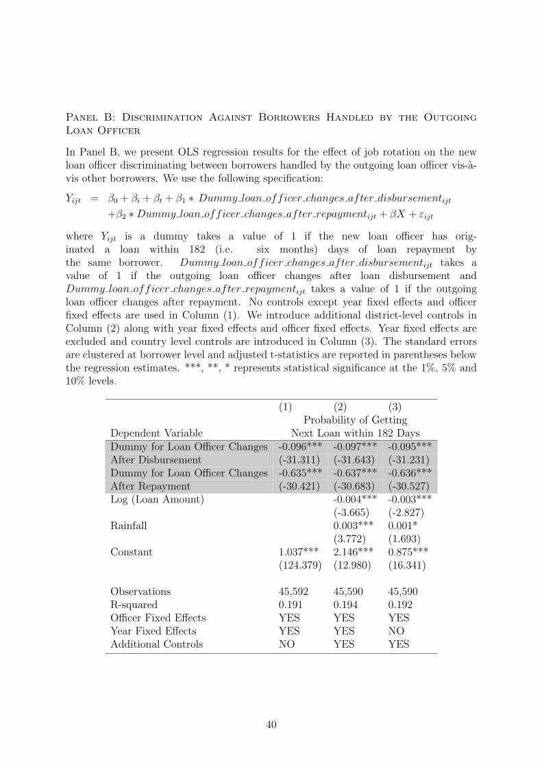
Interestingly, we also find that the (incoming) new loan officer discriminates between

borrowers who borrowed their previous loan during the tenure of the outgoing loan officer

and those who borrowed their previous loan during her tenure: borrowers in the former

4

group have less chance of being given a new loan when compared to borrowers in the

latter group. This evidence suggests that the incoming loan officer anticipates lack of

(screening) effort on the part of the previous loan officer.

The rest of the paper proceeds as follows: Section II describes the literature and

highlights our contribution. Section III provides the institutional background. Section

IV describes a simple model that generates our thesis. Section V describes the data while

Section VI explains our empirical results. Section VII concludes.

II Literature Review

Our study relates to the literature on banking as well as to the organizational eco-

nomics literature that examines the role of information in organizational decision making.

First, our study relates to a growing literature in banking that examines the incentive

effects of loan officers on the quality of lending. We contribute to this literature by high-

lighting the perverse incentives created by job rotation when lending is based on soft

information. In this respect, our study is closest to Hertzberg, Liberti, and Paravisini

(2010), who show that impending loan rotation in a bank creates incentives for the

incumbent agent to reveal information truthfully. The agent faces the threat of being ex-

posed by the incoming agent, which would adversely impact her career prospects. While

Hertzberg, Liberti, and Paravisini (2010) highlight this important benefit of job rotation,

we focus on the costs stemming from job rotation in organizational environments where

soft information dominates decision-making. Because bank lending inherently depends

on soft information, we highlight this cost in the context of a bank.3 In particular, we

focus on agricultural loans provided to small farmers in India — a setting where loans

are made primarily using soft information.

Liberti and Mian (2009) find that hierarchical and geographical distance between

collectors of information and those who use the same in decision making reduce the

importance of soft information in lending. Agarwal and Hauswald (2010) find that del-

egation of authority leads to increased production and utilization of soft information in

decision making. Di Maggio and Van Alstyne (2012) argue that job rotation leads to

destruction of human capital acquired over the years by loan officers, which leads to ad-

verse loan performance. Agarwal and Ben-David (2014) find that change in incentives

from fixed salary to volume-based pay increases aggressiveness of loan origination and

leads to higher default. Cole, Kanz, and Klapper (2013) examine the effect of various

performance-based compensation schemes for loan officers on the quality of lending done

3Among empirical studies that investigate job rotation, Arya and Mittendorf (2004) shows that jobrotation can help a principal to know the true ability of the workers. Job rotation has also been considereda costless way of extracting information about the productivity of a job (Hirao (1993) and Arya andMittendorf (2004)).

5

by loan officers. Berg, Puri, and Rocholl (2013) highlight the perverse incentives created

by volume-based incentives when lending is based on hard information. Specifically, they

find that the quality of lending is adversely affected in such settings because loan officers

increasingly use multiple trials to move loans over the cut-off. Puri, Rocholl, and Steffen

(2010) find that information about borrowers obtained from simple savings or checking

accounts can help to improve loan performance.

Relatedly, our study also contributes to the banking literature that studies the use of

soft versus hard information in bank lending. This literature identifies hard information

with “transactions-based lending.” Berger and Udell (2002), Stein (2002), Petersen and

Rajan (2002), and Berger, Miller, Petersen, Rajan, and Stein (2005), among others,

provide support for this link. Petersen and Rajan (2002), Berger, Miller, Petersen, Rajan,

and Stein (2005), DeYoung, Glennon, and Nigro (2008) and Liberti and Mian (2009),

Agarwal and Hauswald (2010) and Skrastins and Vig (2013) substantiate a positive link

between geographical and hierarchical distance between the bank and the borrower and

the use of hard information.

This study also relates to the literature examining agency problems that arise when

agents have to communicate with each other inside a firm to facilitate decision-making.

We contribute to the organizational economics literature by highlighting the costs of job

rotation when decision making is based on soft information. Aghion and Tirole (1997)

develop a theory of allocation of formal and real authority in an organization. Starting

from the premise that a principal’s preferred project need not be the best choice for the

agent, they show that by delegating authority to an agent the principal loses some control

over the project. However, such delegation increases the agent’s initiative. They also

show that the principal delegates more authority to the agent if the degree of congruence

between the principal’s and agent’s project choices is high. Our study shows that the

congruence between an agent’s preferred actions and those of the principal is low when the

agent finds it imminent that he/she would be rotated out of the job. Thus the agent (loan

officer), whose actions align with the principal’s interests in normal times, deviates from

the principal’s preferred action when job rotation is imminent. This divergence causes

reduction in effort by the agent. The divergence happens in organizational environments

where decision-making relies primarily on soft information because soft information is not

verifiable and the agent realizes that he/she is not going to derive in toto the marginal

benefit/penalty from her effort.

III Background

As institutional background, we describe agricultural lending in India and the nature

of incentives faced by employees of public sector banks in India.

6

III.A Agricultural Lending in India

As described in the introduction, our empirical analysis focuses on the agricultural

loans provided by the lender. Four key factors—soft information, scarce collateral, state

control of banking and poor legal enforcement—characterize the agricultural credit mar-

kets in emerging economies like India.

III.A.1 Importance of soft information

Agricultural lending in a developing country like India is based primarily on soft in-

formation. First, apart from routine information such as name, address, etc., the loan

officer does not have access to any other relevant hard information. Because agricultural

income in India is exempt from income tax,4 small farmers, who do not have any other

source of income other than agricultural income, do not file income tax returns. Neither

is there any independent audit of the farmers’ income. Given that nearly 44.1% of small

farmers in India are illiterate (Mahadevan and Suardi, 2013), proper annual records of

production are not maintained by small farmers. As well, no publicly available credit

history exists for borrowers of agricultural loans in India.5 The farmers in our sample are

quite small: they have landholding of less than 2 hectares. In fact, nearly 82% farmers in

India have landholding less than 2 hectares (Mahadevan and Suardi, 2013). Small farmers

do not use modern technology as these involve fixed costs both in terms of learning and

financial resources. Given the size of their landholdings, such fixed costs are dispropor-

tionately high. Nearly 65% of the small farmers depend on rain fed irrigation (Mahadevan

and Suardi, 2013). As well, more than 75% of Indian farmers are not even covered by

crop insurance (Mahul and Verma, 2012). Thus, a loan officer cannot use potentially

hard information such as the use of irrigation and/or crop insurance. This deprives the

loan officer of any “verifiable” source of information to assess the creditworthiness of an

agricultural borrower.

Second, the literature on soft versus hard information argues that distance—both and

hierarchical—determines crucially the use of hard versus soft information (see Petersen

and Rajan (2002), Berger, Miller, Petersen, Rajan, and Stein (2005), Liberti and Mian

(2009), Agarwal and Hauswald (2010) among others). We have observed during the

data collection exercise that the branch manager, who is the loan officer in our sample,

meets all the borrowers personally before sanctioning crop loans. The branch manager

is located geographically proximate to the borrower and interacts regularly with them.

Also, as part of the policy set by the bank, loans below the size of INR 0.65 million can

4As per Sec 10(1) of the Income Tax Act 1961, agricultural income is exempt from tax.5 India has a credit information bureau named “Credit Information Bureau (India) Limited (CIBIL).”

CIBIL needs a unique identifier such as a social security number, income tax number, etc. to link atransaction to an individual. No such unique identifier exists for small and marginal farmers. Therefore,CIBIL does not possess the credit histories of small agricultural borrowers.

7

be sanctioned by the branch manager. Because the size of the agricultural crop loans

in our sample are much smaller, the loan officer has the authority to sanction the small

sized agricultural crop loans without having to seek the permission of an officer higher in

the organizational hierarchy.

Finally, the borrowers in our sample do not own a checking or savings account with

the bank. This fact reflects the reality of financial exclusion in India where 51% of farmers

do not even have a bank account (Karmakar 2012). The loan officers interactions with

his borrowers are through the loan account and transactions related to the same. As a

result, unlike in Puri, Rocholl, and Steffen (2010), loan officers cannot utilize information

from savings or checking accounts to obtain hard information about the borrower.

III.A.2 Scarce collateral

A common solution to mitigate strategic default is to have the borrower post a physical

asset, which can be appropriated upon default. However, most farmers in emerging

economies are too poor to post any substantial collateral other than the land and the

crop. Also, poorly delineated property rights over land exacerbate the problem by making

it difficult for the bank to foreclose the land that has been put up as collateral for the loan.

Moreover, foreclosing a farmer’s land is extremely politically sensitive as local politicians,

cutting across party lines, intervene on behalf of farmers.6 In extreme cases, laws have

been passed to render recovery of agricultural loans difficult; an example of this is the

Andhra Pradesh Microfinance Institutions (Regulation and Moneylending) Act, 2010.

Effectively, farmers in India do not face the threat of their land being taken over by their

lenders, which encourages strategic default.

III.A.3 State controlled banking system

Government of India plays a dominant role in the banking sector. Government owned

banks account for 74.2% (75.1%) of aggregate amount loans outstanding (deposits) in the

banking sector. The Government of India nationalized many private banks in 1969 and

1980 and enforced several measures with the declared objective of improving access to

finance to some “critical” sectors and to vulnerable sections of the population. Priority

sector guidelines and branch expansion norms were the most impactful regulations issued

(see Burgess and Pande (2003), Burgess, Pande, and Wong (2005), Cole (2009)). Priority

sector lending guidelines require by law that 18% of a bank’s credit be directed to agri-

culture and allied activities. Government of India introduced another set of guidelines

that required the banks to open branches in four unbanked locations for every branch in

a banked location. This substantially increased the branch network and improved access

6In one such incident in Mysore, Karnataka, the lender was forced to return the tractor repossessedfrom a farmer as the farmer committed suicide. The local politicians alleged that the suicide was due to“arm twisting“ tactics employed by the recovery agents of the bank. The Hindu, June 30, 2008.

8

to finance in rural areas (see Burgess and Pande (2003)). As on 31st March, 2013, there

were 157 commercial banks operating 104,467 branches in India.7

III.A.4 Poor enforcement

Given state control of banking and the political economy of state controlled lending

(see Khwaja and Mian (2005), Cole (2009)), recovery of loans has been a major chal-

lenge in India. Though the establishment of debt recovery tribunals and the passage

of “Securitization and Reconstruction of Financial Assets and Enforcement of Security

Interest( SARFAESI)” Act have substantially improved the NPA scenario (see Visaria

(2009), Vig (2013)), neither of them apply to small agricultural loans. Thus, when it

comes to agricultural loans, lenders do not have recourse to any special laws and have to

rely on courts for enforcement. However, the slow judicial process compounds lenders’

difficulties in loan recovery.8

III.B Loan Officer Incentives in Indian Public Sector Banks

For employees of public sector banks in India, who are considered as “public ser-

vants”,9 the number of years spent on the job remains the most important factor that

determines the promotion of a loan officer in Indian public sector banks.

The Ministry of Finance, Government of India decides the compensation for em-

ployees of public sector banks; this compensation varies primarily based on the level of

an employee in the organizational hierarchy. Unlike their counterparts in the private

sector banks, employees in public sector banks do not receive variable pay linked to per-

formance. Moreover, the level of compensation provided to employees of public sector

banks is significantly lower than that provided to employees of private sector banks, whose

compensation is primarily market-driven.10 Banerjee, Cole, and Duflo (2008) document

that loan officers in Indian public sector banks are driven more by fear of prosecution by

the federal vigilance authorities for alleged corruption than by positive rewards related to

their performance. Such a skewed incentive structure typically motivates the loan officers

to be lax in their effort when the perceived threat of being prosecuted is low. As we ar-

gue in section IV, scheduled rotation represents one such instance where the loan officers

7Source:http://rbidocs.rbi.org.in/rdocs/Publications/PDFs/00QSB170913F.pdf8World Bank’s doing business survey 2012-2013 ranks India 132 out of 185 in terms of ease of doing

business. In terms of enforcement of contracts India occupies 17th out of 185 countries surveyed. Also,in India it takes on an average 1420 days to enforce a contract. In comparison in Singapore the sametakes just 150 days.

9See http://en.wikipedia.org/wiki/Gazetted Officer (India)10The Central Bank governor is on record saying that the salaries of public sector executives

are far lower compared to the remuneration received by their private sector counterparts. Source:http://profit.ndtv.com/news/market/article-rbi-for-higher-salaries-to-ceos-of-psu-banks-41347 In fact,the chairman of largest bank in India, which is a public sector bank, draws a total remuneration lessthan 20% of what her counterparts in the private sector draw.

9

know ex-ante that they cannot be held fully responsible for ex-post loan performance on

loans lent towards the end of their tenure.

Indian public sector banks follow a common system of performance appraisal for their

employees. As specified in the pro-farma appraisal document issued by the Department

of Financial Services, Ministry of Finance, Government of India, a loan officer in a public

sector bank in India is evaluated on three dimensions:

1. Business Issues: This category, which gets a weightage of 60%, includes aspects such

as lending, NPA management, resource mobilization, selling third-party products

such as insurance and mutual funds, income and expense management, etc. These

quantitative aspects are measured against set targets.

2. Qualitative aspects: This category includes qualitative aspects such as proper main-

tenance of books, remarks during audit, compliance of audit instructions, customer

service, cleanliness of branch premises, employee satisfaction. Here, the supervising

manager decides a rating based on his/her subjective assessment of the employee’s

performance on these criteria. This category gets a weightage of 10%.

3. Managerial Qualities: In this category, , which gets a weightage of 30%, the loan

officer is evaluated for his/her leadership skills, administrative acumen, decision

making, communication skills, etc. Here again the supervising manager assigns a

score based on his/her subjective assessment of the loan officer.

If a loan officer’s performance is rated as below average by the bank, then chances

of promotion gets substantially diminished even if the officer has spent many years at

the same level. However, a very high rating does not necessarily qualify an officer for

promotion unless he/she has spent the required number of years at the particular level

of the organizational hierarchy.

From our perspective, a couple of features of the incentives system are worth noting.

First, assessment of the loan officers performance is based only by his/her achievements

in the current branch. The loan officer’s performance in branches he/she previously

served has no bearing on his/her current appraisal ratings. The appraisal document only

requires the loan officer to provide details about the previous positions held. Second,

NPA management receives an overall weightage of only 10%.

IV A Simple Model

We develop a simple model to derive our empirical hypotheses. Consider a principal-

agent relationship, where a bank is the principal and loan officer(s) are the agents. We

study how the effort choice of the loan officer(s) is affected by job rotation when decision-

making inside the firm is driven by soft information. We study this question given the

10

incentive structure set by the principal. Therefore, we take the incentive contract, which

the principal decides to incentivize the loan officers, as exogenously given and then ex-

amine how job rotation affects the loan officer’s effort. Specifically, we assume that the

incentive structure is identical across loans that are not affected by job rotation and loans

that are affected by job rotation. Apart from our focus being on how effort choice is af-

fected by job rotation, this assumption is justified on conceptual and practical grounds.

Conceptually, as discussed in the introduction, when the information collected by the em-

ployee is soft, neither the information nor the effort at collecting the same can be verified.

In this case, as in Holmstrom and Milgrom (1991) the number of observables—default

on the loan in this case—is less than the number of activities performed by two different

agents. Therefore, the firm cannot design an incentive contract that rewards each em-

ployee partially according to this effort. Moreover, the empirical setting we study—an

Indian public sector bank where the incentives are quite low powered—involves a princi-

pal that does not alter the incentive structure for loans affected by job rotation vis-a-vis

loans that are not affected by job rotation.

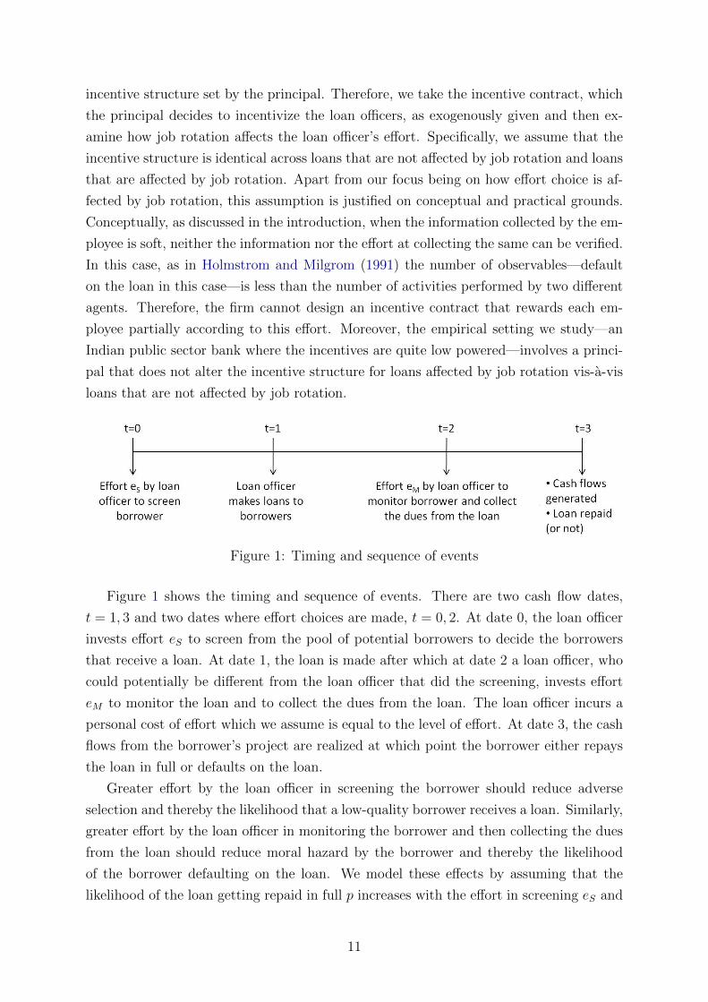
Figure 1: Timing and sequence of events

Figure 1 shows the timing and sequence of events. There are two cash flow dates,

t = 1, 3 and two dates where effort choices are made, t = 0, 2. At date 0, the loan officer

invests effort eS to screen from the pool of potential borrowers to decide the borrowers

that receive a loan. At date 1, the loan is made after which at date 2 a loan officer, who

could potentially be different from the loan officer that did the screening, invests effort

eM to monitor the loan and to collect the dues from the loan. The loan officer incurs a

personal cost of effort which we assume is equal to the level of effort. At date 3, the cash

flows from the borrower’s project are realized at which point the borrower either repays

the loan in full or defaults on the loan.

Greater effort by the loan officer in screening the borrower should reduce adverse

selection and thereby the likelihood that a low-quality borrower receives a loan. Similarly,

greater effort by the loan officer in monitoring the borrower and then collecting the dues

from the loan should reduce moral hazard by the borrower and thereby the likelihood

of the borrower defaulting on the loan. We model these effects by assuming that the

likelihood of the loan getting repaid in full p increases with the effort in screening eS and

11

the effort in monitoring the loan and collecting the dues eM :

p ≡ p (eS, eM) , (1)

pi > 0, pii < 0, i = 1, 2,

where the subscripts denote partial derivatives. We also assume that the effort in screen-

ing and the effort in monitoring and collecting the dues are either complementary to each

other (p12 ≥ 0) or substitutes for each other (p12 = 0):

p12 ≥ 0 (2)

Bank lending relies on relationships and soft information (Petersen (2004); Ramakrishnan

and Thakor (1984)). In the Indian context, it has been shown that informal relationships

between a loan officer and a borrower play a major role in lending and repayment de-

cisions (Fisman, Paravisini, and Vig, 2012). Therefore, the effort invested in screening

and monitoring are primarily aimed at collecting soft information about the borrower.

Therefore, we assume the effort to be observable but not verifiable. This assumption dif-

fers from that in Hertzberg, Liberti, and Paravisini (2010), who show that the outgoing

loan officer reports truthfully near the scheduled rotation because she fears being exposed

by the incoming loan officer. Such exposure is possible when the incoming loan officer can

uncover the information the outgoing loan officer chooses to hide. However, uncovering

soft information hidden by the outgoing loan officer poses difficulties.

As argued above, we consider incentive contracts for loan officers as exogenously

specified. Following the discussion in Section III.B, we model low-powered incentives

that reward performance and penalize default:

wp > wd, (3)

where wp denotes the payoff to the loan officer when the borrower repays the loan in full

and wd denotes the payoff to the loan officer when the borrower defaults on the loan.

IV.A Job Rotation

In a bank, with respect to loans affected by job rotation, the outgoing and incom-

ing officers become jointly responsible for the performance of such a loan. While the

outgoing loan officer is responsible for screening and due diligence at the time of lend-

ing, the incoming officer bears responsibility for residual monitoring and collecting the

dues. This creates a situation of moral hazard in teams (Holmstrom, 1982), where neither

the outgoing loan officer nor the incoming loan officer can be held fully responsible for

the performance of the loan. We model this by assuming that payoff to the outgoing

12

loan officer equals (α · wp, α · wd) while the payoff to the incoming loan officer equals

([1 − α] · wp, [1 − α] · wd) , where 0 < α < 1.

IV.B Analysis

We solve the model by backward induction by considering separately the “job rota-

tion” and “no job rotation” scenarios. First consider the case under “no job rotation.”

When the loan officer is solely responsible for the performance of the loan and does the

screening, monitoring and collection of dues on his own, his expected payoff is given by:

U (eS, eM) = wp · p (eS, eM)︸ ︷︷ ︸borrower repays loan in full

+ wd · [1 − p (eS, eM)]︸ ︷︷ ︸borrower defaults on the loan

− eS − eM (4)

The loan officer decides his screening and monitoring effort to maximize his expected

payoff. Using backward induction, given the effort in screening chosen by the loan officer,

he chooses monitoring effort to maximize his expected payoff:

eN−JRM = max

eMU(eN−JRS , eM

)(5)

where the N − JR denotes effort choice in the “no job rotation” case. The loan officer

then chooses screening effort to maximize his expected payoff:

eN−JRS = max

eSU(eS, e

N−JRM

)(6)

The first-order conditions for the effort choice are therefore given by:

p1

(eN−JRS , eN−JR

M

)= p2

(eN−JRS , eN−JR

M

)=

1

wp − wd

(7)

Now consider the “job rotation” case. As stated above, the outgoing loan officer is

responsible for screening while the incoming officer is responsible for monitoring and

collecting the dues. Therefore, the expected payoff to the outgoing loan officer UO is

given by:

UO (eS, eM) = αwp · p (eS, eM) + αwd · [1 − p (eS, eM)] − eS (8)

The expected payoff to the incoming loan officer U I is given by:

U I (eS, eM) = [1 − α]wp · p (eS, eM) + [1 − α]wd · [1 − p (eS, eM)] − eM (9)

13

Given the effort in screening chosen by the outgoing loan officer, the incoming loan officer

chooses (monitoring) effort to maximize his expected payoff:

eJRM = maxeM

U I(eJRS , eM

)(10)

where the superscript JR denotes effort choice in the “job rotation” case. Anticipating

the monitoring effort of the incoming loan officer, the outgoing loan officer chooses effort

to maximize his expected payoff:

eJRS = maxeS

UO(eS, e

JRM

)(11)

The first-order conditions for the effort choice in the “job rotation” case are therefore

given by:

p1

(eJRS , eJRM

)=

1

α (wp − wd)(12)

p2

(eJRS , eJRM

)=

1

(1 − α) (wp − wd)(13)

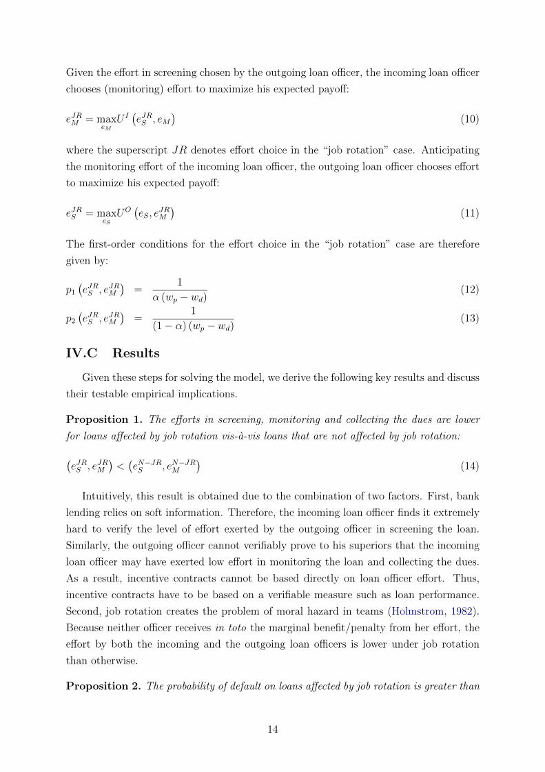
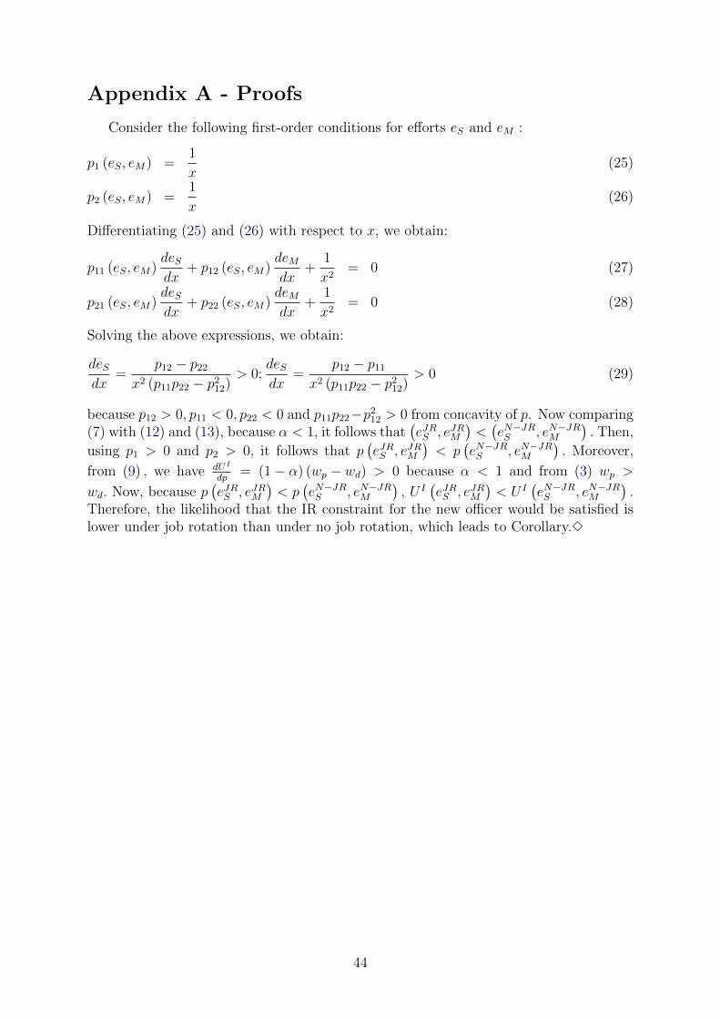
IV.C Results

Given these steps for solving the model, we derive the following key results and discuss

their testable empirical implications.

Proposition 1. The efforts in screening, monitoring and collecting the dues are lower

for loans affected by job rotation vis-a-vis loans that are not affected by job rotation:

(eJRS , eJRM

)<(eN−JRS , eN−JR

M

)(14)

Intuitively, this result is obtained due to the combination of two factors. First, bank

lending relies on soft information. Therefore, the incoming loan officer finds it extremely

hard to verify the level of effort exerted by the outgoing officer in screening the loan.

Similarly, the outgoing officer cannot verifiably prove to his superiors that the incoming

loan officer may have exerted low effort in monitoring the loan and collecting the dues.

As a result, incentive contracts cannot be based directly on loan officer effort. Thus,

incentive contracts have to be based on a verifiable measure such as loan performance.

Second, job rotation creates the problem of moral hazard in teams (Holmstrom, 1982).

Because neither officer receives in toto the marginal benefit/penalty from her effort, the

effort by both the incoming and the outgoing loan officers is lower under job rotation

than otherwise.

Proposition 2. The probability of default on loans affected by job rotation is greater than

14

on loans not affected by job rotation:

p(eJRS , eJRM

)< p

(eN−JRS , eN−JR

M

)(15)

This result follows from the probability of default on the loan increasing with the

effort in screening and the effort in monitoring the loan.

Corollary 1. The likelihood of the incoming loan officer providing a repeat loan to a

borrower screened by the outgoing loan officer is lower than the situation in which the

repeat borrower is screened by the same officer.

This result follows from the incoming loan officer accounting for the possibility that the

effort made by the outgoing officer in screening loans (that are affected by job rotation)

would be lower than the (screening) effort that she would herself would make in screening

the borrowers.

IV.D Empirical Implications

The main empirical implication follows from proposition 2, which implies that loans

that are affected by job rotation are more likely to default when compared to loans that

are not affected by job rotation. Proposition 1 specifies that the mechanism underlying

this effect is that loan officers exert lower effort in screening, monitoring and collecting

the dues for a loan affected by job rotation when compared to a loan that is not affected

by job rotation. Corollary 1 provides the final empirical implication: because of the lower

effort in screening by the outgoing loan officer, the incoming loan officer is likely to ration

credit to borrowers that were screened by the outgoing loan officer.

V Data

For our empirical analysis in the paper, we use loan account level information from an

Indian public sector bank.11 The bank provided us data for 15 branches located in four

districts in the state of Andhra Pradesh, two districts in Karnataka, and three districts

in Maharashtra. The details regarding the names of districts and the location of the

branches are provided in Appendix 1. The loan account data provided to us by the bank

starts in October 2005 and ends in May 2012. However, as described in the introduction,

to avoid the problem of right censoring of data on loan performance for the loans issued

later in our sample, we restrict our analysis to loans issued till May 2011.

We have data pertaining to more than 45,000 loans availed by more than 16,000

agricultural borrowers. These loans were issued by 51 different loan officers who managed

11The bank has a history of more than 75 years. The bank has pan India presence. It operates throughmore than 1000 branches.

15

the 15 branches during our sample period. We obtain information regarding the identity

of the loan officer who lent a particular loan and the tenure of the loan officer in a

particular branch. We have hand collected this information by verifying bank records.

For the purpose of this paper, the loan officer corresponds to the branch manager.

The transaction records provided by the bank include the date of each transaction, a

short description of each transaction, transaction amount, type of transaction (debit or

credit), the account balance before and after the transaction and type of balance (debit

or credit). With help of the account details provided to us by the bank, we are able

to infer when a loan was availed, number of days the loan was outstanding, the interest

charged etc. All the loans analyzed are crop loans with a one year maturity.12

Dependent variable: We define default as the borrower not repaying the loan by the

due date of repayment. In using this definition of default, we follow the Reserve Bank

of India’s guidelines for Asset Classification, Provisioning and Other Related Matters,

which stipulate that a loan is considered in default if it has not been repaid by the due

date of repayment. Our results remain qualitatively and quantitatively unchanged when

we define default as the borrower not having repaid the loan 90 days after scheduled

repayment, which corresponds to the Reserve Bank of India’s norm for classification of

loans into non-performing assets.13

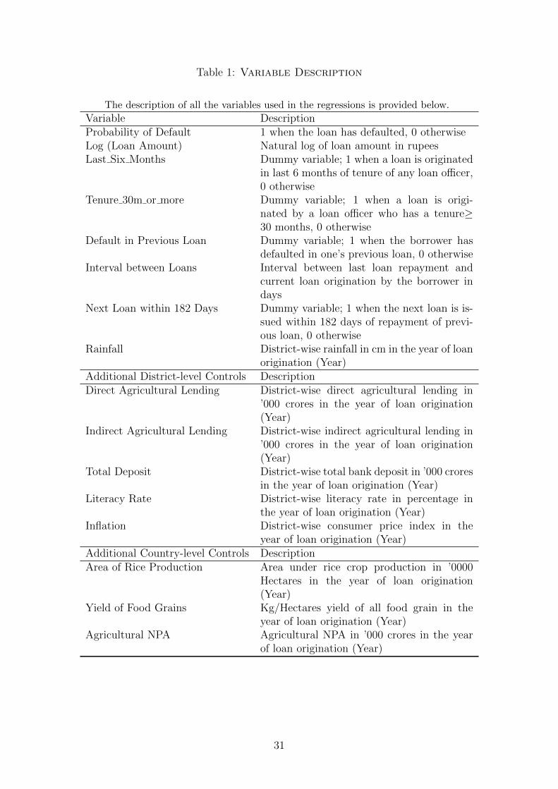
Control variables: We use the following controls in our econometric analysis. Rainfall

data pertains to district-wise yearly rainfall in the year of loan origination (year here-

after). This data is taken from the Indian Meteorological Department (www.imd.gov.in).

Data for direct and indirect agricultural lending and for the total deposits in a (dis-

trict, year) are obtained from the Reserve Bank of India (RBI) Database on Indian

Economy (www.dbie.rbi.org.in). Data for the literacy rate in a (district, year) is ob-

tained from the Indian census data. Inflation is measured as the district-wise yearly

consumer price inflation; the data for the same is obtained from the Indian Labour Bu-

reau (www.labourbureau.nic.in). Area of rice production refers to area under rice crop

production in ’0000 hectares in a year; this data is obtained from the Indiastat database

(www.indiastat.com). Yield of food grains is defined as Kg/Hectares yield of all food

grain in a year; we obtain this data from www.agricoop.nic.in. Data for the nonperform-

ing assets (NPA) for each year at the country level is obtained from the RBI website.

Table 1 provides a brief description of all the variables used in this study.

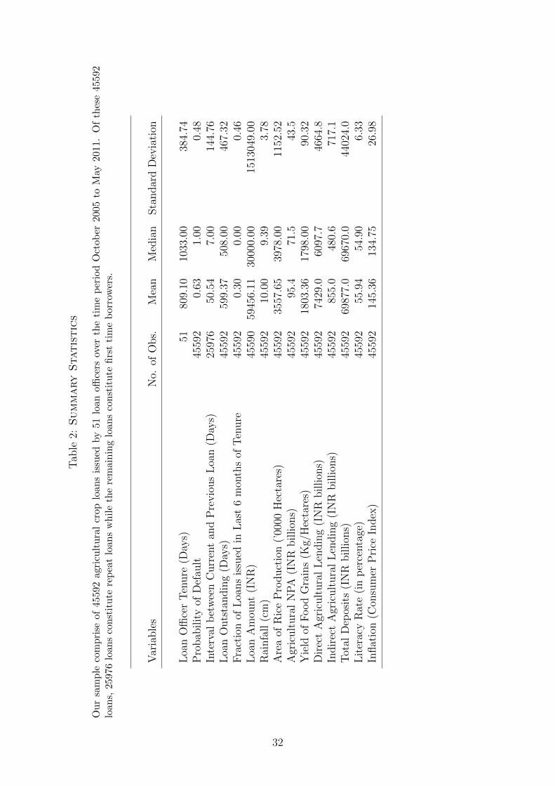
V.A Descriptive Statistics

Table 2 provides the descriptive statistics for the variables employed in our study.

Loan officer tenure equals an average of 809 days, or 2.2 years, while the median equals

12A copy of the loan agreement between the bank and borrowers of agricultural loans, which capturesthe various features of the loan contract, is available from the authors on request.

13See Section 2.1 in http://www.rbi.org.in/scripts/bs viewmascirculardetails.aspx?id=7370#cla.

16

1033 days, or 2.8 years. The probability of default for a loan in our sample, which consists

exclusively of agricultural crop loans, is on average 63%. The median loan in our sample

does not meet the payment obligations by the scheduled repayment date. While such a

large rate of default may be surprising in the context of a developed economy, because

of the challenges related to agricultural lending described in section III, high default

rates on agricultural loans represent a key concern in developing countries such as India.

In fact, concerned with the dismal performance of the agricultural sector and rising

farmer suicides because of indebtedness,14 Government of India set up a high powered

committee (The Radhakrishna Committee) in 2007 to study the problem of agricultural

distress and high indebtedness and suggest remedial measures. Moreover, as part of

the financial budget speech delivered on February 29, 2008, the then Finance Minister

of India announced an unprecedented bailout of indebted small and marginal farmers,

which increases the rate of default in our sample. However, the empirical strategy we

adopt, which exploits staggered transfers of loan officers all through our sample, ensures

that the debt waiver scheme does not affect our results.

Table 2 also shows that of the 45592 loans in our sample, approximately 57% (=25976

loans) are given to repeated borrowers. We also notice that on average 30% of the loans

are given by a loan officer during the last six months of his/her tenure while the median

loan is given earlier. The average loan amount equals INR 59456 or approximately $1000

while the median loan amount equals INR 30,000 or approximately $500.

VI Results

VI.A Empirical Strategy

Our empirical strategy critically depends on loan officer rotation being well-defined

and being unrelated to the loan officer’s performance. A well-defined loan officer rotation

policy also gives an opportunity to the loan officer to plan her moves in advance.

Public sector banks in India follow a uniform policy of rotating their loan officers after

three years.15 Accordingly, the large public sector bank that has provided us with the data

follows the same policy. Because the Government of India only issues broad guidelines

relating to rotation and promotion of loan officers, banks exercise some discretion in

transferring officers before they complete three years or in retaining officers in a branch

even after completing three years. Our discussions with the management of the bank

14According to a UN report, more than 100,000 farmers have committed suicide since 1997, 87% ofthem incurring an average debt of US$835.

15See for example the documents detailing the rotation policies of three largepublic sector banks—Punjab National Bank: http://getup4change.org/rti/wp-content/uploads/2012/01/Transfer-policy-for-officers.htm; State Bank of India:http://www.sbioahc.com/business%20company files/circulars/assn%202013/circular%20no.11.pdf;and Uco Bank: http://www.aiucbof.com/transfer promotion.php?type=Transfer Promotion.

17

and our review of official documents reveal that administrative exigencies such as acute

shortage of officers in a branch/region, death/long illness of a loan officer in a branch,

etc. primarily contribute to early transfers (i.e. before completion of three years). On

the other side of the spectrum, because a loan officer has to wait for a replacement to be

identified and for the replacement to takeover responsibilities from him, which leads to

many loan officers’ tenure being more than three years.

However, loan officer transfers are unrelated to performance. All officers are members

of All India Bank Employees union, which strongly resists any move which is seen by the

employees as arbitrary. Due to the potential pressure from the unions, managements of

public sector banks play it safe and stick to a uniform transfer policy.

As mentioned in the introduction, in figure 2, we plot the probability of a loan officer

continuing in her current job in the (n + 1)th month conditional on having been on the

job for n months. In this figure, we observe a sharp discontinuity at three years in the

probability of a loan officer continuing in her current job. Therefore, we find that the

bank’s rotation policy of transferring officers after three years is indeed operational on

the ground. Figure 3 shows the distribution of loans based on loan officer tenure. We

notice here that close to 45% of the loans are originated by loan officers who spend exactly

three years in the branch. Moreover, in figures 2 and 3, we find sufficient variation in

loan officer tenure around the three-year threshold, which enables us to identify the effect

of job rotation on loan performance.

Our empirical strategy also exploits the fact that the sample of agricultural crop loans

given by the bank have a fixed maturity of one year, which enable us to cleanly separate

officers into “treatment” and “control” groups to estimate the effect of a rotation policy.

Using these groups, we estimate a difference-in-difference effect of the rotation policy.

To fix ideas, consider a representative loan officer who completes two-and-a-half years in

a branch. Because the expected tenure is three years, she can expect to be transferred

from the branch in the next six months. So, loans that she originates in the next six

months are likely to be due during the tenure of the loan officer that replaces her. Thus,

complete responsibility for the performance of the loans that she originates in the last six

months of her tenure cannot be attributed to her. Moreover, given the soft information

that drives bank lending, the incoming loan officer cannot verify the effort that she made.

As a result, this group constitutes the treatment group for examining the effect of job

rotation. In contrast, consider a representative loan officer who has not completed two-

and-a-half years in the branch. Because she does not expect to be transferred over the

next six months, she is likely to be held fully responsible for loans that she originate in

these next six months. Such an officer forms part of our “control” group.

We estimate the difference-in-difference as follows. For the treatment group of officers,

we first estimate the difference between average default rates for loans originated in the

last six months of their tenure vis-a-vis the average default rate for loans originated in

18

previous periods. Next, we estimate the same difference for the control group of officers.

The difference between these two differences provides a causal estimate of the effect

of job rotation on loan performance. This is because the second difference provides an

estimate for the counterfactual question: what would have been the default rate if the

representative loan officer had originated a loan that was not affected by job rotation?

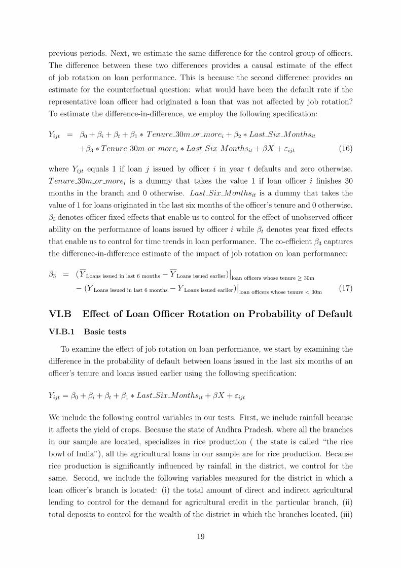
To estimate the difference-in-difference, we employ the following specification:

Yijt = β0 + βi + βt + β1 ∗ Tenure 30m or morei + β2 ∗ Last Six Monthsit

+β3 ∗ Tenure 30m or morei ∗ Last Six Monthsit + βX + εijt (16)

where Yijt equals 1 if loan j issued by officer i in year t defaults and zero otherwise.

Tenure 30m or morei is a dummy that takes the value 1 if loan officer i finishes 30

months in the branch and 0 otherwise. Last Six Monthsit is a dummy that takes the

value of 1 for loans originated in the last six months of the officer’s tenure and 0 otherwise.

βi denotes officer fixed effects that enable us to control for the effect of unobserved officer

ability on the performance of loans issued by officer i while βt denotes year fixed effects

that enable us to control for time trends in loan performance. The co-efficient β3 captures

the difference-in-difference estimate of the impact of job rotation on loan performance:

β3 = (Y Loans issued in last 6 months − Y Loans issued earlier)∣∣loan officers whose tenure ≥ 30m

− (Y Loans issued in last 6 months − Y Loans issued earlier)∣∣loan officers whose tenure < 30m

(17)

VI.B Effect of Loan Officer Rotation on Probability of Default

VI.B.1 Basic tests

To examine the effect of job rotation on loan performance, we start by examining the

difference in the probability of default between loans issued in the last six months of an

officer’s tenure and loans issued earlier using the following specification:

Yijt = β0 + βi + βt + β1 ∗ Last Six Monthsit + βX + εijt

We include the following control variables in our tests. First, we include rainfall because

it affects the yield of crops. Because the state of Andhra Pradesh, where all the branches

in our sample are located, specializes in rice production ( the state is called “the rice

bowl of India”), all the agricultural loans in our sample are for rice production. Because

rice production is significantly influenced by rainfall in the district, we control for the

same. Second, we include the following variables measured for the district in which a

loan officer’s branch is located: (i) the total amount of direct and indirect agricultural

lending to control for the demand for agricultural credit in the particular branch, (ii)

total deposits to control for the wealth of the district in which the branches located, (iii)

19

literacy to control for awareness of modern methods of farming that can affect agricultural

production, (iv) inflation as it directly affects the borrowers’ consumption basket. We

also include other control variables that are measured yearly at the country level: (i) total

area under rice production, (ii) average yield of food grains, and (iii) total nonperforming

assets among agricultural loans.

The results for these tests are presented in table 3. In Column (1), we do not include

any control variables except for the year and officer fixed effects. In column (2), we

introduce all the district/loan level control variables described above. For brevity, we

report the coefficients of log(loan amount) and rainfall in the district because these are

the variables that are statistically significant. We find that log(loan amount) is positively

correlated with the probability of default, which is consistent with the likelihood of default

being greater when the borrower is more indebted. We also find that rainfall in the district

is positively correlated with the probability of default. This could possibly be the case

because excessive rainfall adversely affects rice production and could therefore lead to

borrower distress. In column (3), we include control variables that are measured at the

country level: area under rice production, yield of food grains, and agricultural NPA.

Because these variables vary at the yearly level, we exclude year fixed effects from the

specification though the district/loan level control variables as well as officer fixed effects

continue to be included.

Across columns (1)-(3) of table 3, we notice that the coefficient estimate for β1 is

positive and statistically significant at the 1% level. Thus we find that the loans issued

in the last six months of and officer’s tenure default more than loans issued earlier.

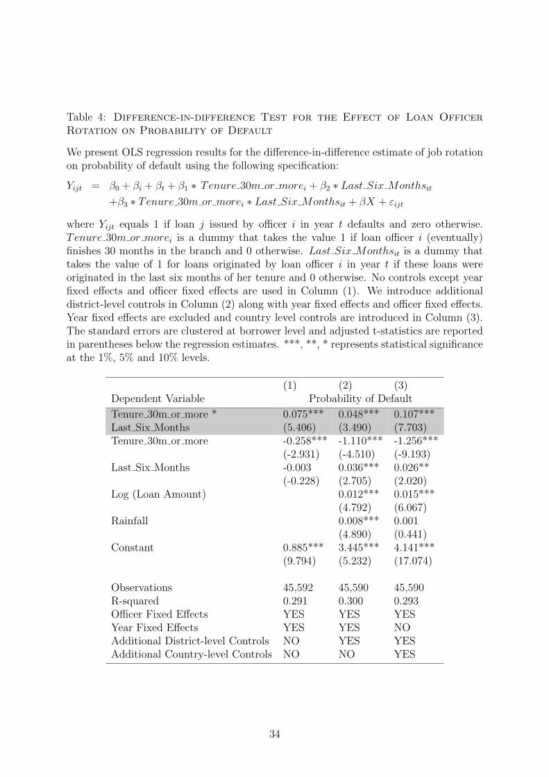
VI.B.2 Difference-in-difference

The above tests do not enable us to control for the effect of confounding factors. For

example, the higher default rates in the last six months of an officer’s tenure could be

because the new officer that replaces him faces a learning curve as in Di Maggio and

Van Alstyne (2012). To disentangle the effect of job rotation from this alternative, we

employ the empirical strategy using difference-in-difference tests described above.

Because the loan officers in the treatment group can anticipate an impending transfer,

they can plan their moves in advance. Loan officers in the control group, who experience

unscheduled transfers, cannot do so. Thus, while the effect of the new officer facing a

learning curve should manifest in both the control and treatment groups, the effect of

job rotation should be visible only in the case of the treatment group. We therefore test

equation (25) now; the results for these tests are presented in table 4. The specifications

shown in columns (1)-(3) of table 4 are similar to those in table 3.

Across all three specifications, we observe that the coefficient estimate for β3 is positive

and statistically significant at the 1% level, which shows that the difference-in-difference

20

estimate for the effect of job rotation on the probability of loan default is positive. Eco-

nomically, using the coefficient estimate for β3 in column (1) we infer that loans that

are affected by job rotation default 7.5% more than loans that are not affected by job

rotation.

Across columns (1)-(3) of table 4, we notice that the coefficient estimate for β2, which

provides an estimate of the probability of default for loans originated in the last six

months of any officer’s tenure vis-a-vis the probability of default for loans originated

earlier, is positive and statistically significant at the 5% level or lower in columns 2 and

3. Thus, apart from the difference-in-difference estimate, we find that loans issued in the

last six months of an officer’s tenure default more often than loans issued earlier.

VI.B.3 Effect of learning

Across columns (1)-(3) of table 4, we notice that the coefficient estimate for β1 is

negative and statistically significant at the 1% level. Thus, the loans originated by loan

officers that spend 2.5 years or more in a particular branch have a lower probability of

default when compared to loans originated by officers that spend less than 2.5 years in a

particular branch. Thus, longer tenure has the overall effect of reducing default rate on

loans. As loan officers learn more and acquire soft information about the borrowers, the

portfolio quality improves.

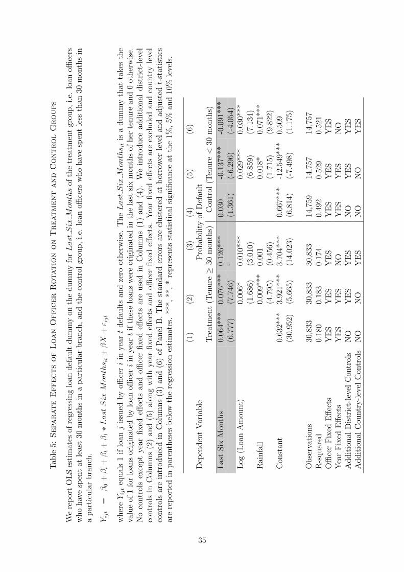
VI.B.4 Examining the effects separately for treatment and control groups

In table 5, we examine the effect of job rotation separately for the treatment and

control groups. In columns (1)-(3) of table 5, we notice that that the coefficient of the

dummy for last six months of tenure is positive and statistically significant at the 1% level.

In contrast, in columns 3 to 6 of table 5, we notice that the coefficient of the dummy for

last six months of tenure is negative and statistically significant in columns 5 and 6 even

though it is insignificant in column 4. Thus, consistent with our hypothesis, job rotation

increases the probability of default on loans originated by the treatment group of loan

officers. However, consistent with learning on the job, the probability of default on loans

originated is lower in the last six months of tenure for the control group of officers.

Also, as we argued in the introduction, the negative coefficients for the control group

suggest that the higher default rates observed in table 4 are not due to a new loan officer

facing a learning curve as in Di Maggio and Van Alstyne (2012). If that were the case, we

should have observed an increase in the default rates in the last six months for the control

group as well. Thus, we can infer that the expertise gained on the job reduces default

rates for loans issued in the last six months for the control group while the hypothesized

effect of job rotation increases the same for the treatment group.

21

VI.C Disentangling possible effects of hard information

Our hypothesis relies on job rotation leading to lower effort in gathering of soft infor-

mation by loan officers. As argued in Section III.A, loan officers have to primarily rely

on soft information for their lending decisions on agricultural crop loans. Therefore, our

empirical setting makes it possible that the above effect of job rotation stems from lower

effort in collecting soft information. Nevertheless, we would like to examine further if

the above results are indeed stemming from lower effort in collecting soft information.

In particular, because default on a loan represents a verifiable outcome and each bank is

likely to maintain a record of defaulters, the above results could still be due to the effect

of job rotation on collection of hard information. However, if the above effects were due

to hard information, then as in Hertzberg, Liberti, and Paravisini (2010), the likelihood

of default on loans affected by job rotation should be lower, not higher as we find.

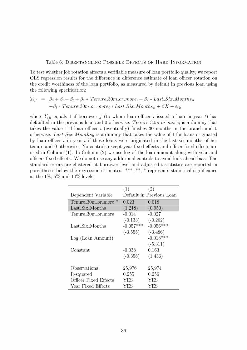
A loan officer does not have to gather any soft information to verify whether or not

a loan applicant has repaid the previous loan within the term specified in the contract.

To test whether job rotation affects a verifiable measure of loan portfolio quality, we

implement the following specification:

Yijt = β0 + βi + βt + β1 ∗ Tenure 30m or morei + β2 ∗ Last Six Monthsit

+β3 ∗ Tenure 30m or morei ∗ Last Six Monthsit + βX + εijt (18)

where Yijt now measures whether borrower j (to whom loan officer i gave a loan in year

t) has defaulted on a previous loan or not. Yijt equals 1 if borrower j has defaulted on a

previous loan and 0 otherwise. By construction, this test is run on the sample of repeat

borrowers. The results are presented in table 6. Column (1) shows the results of the

specification containing year and officer fixed effects while column (2) shows the results

of the specification containing year and officer fixed effects as well as the log of the loan

amount. Loan portfolio quality on average improves in the last 6 months of a loan officer’s

tenure as seen in the negative and statistically significant coefficient estimate for β2, which

suggests that a loan officer is less likely to lend to a previously defaulted borrower in the

last six months of his tenure for fear of leaving verifiable evidence of a dubious loan. The

coefficient estimate for β1 is statistically insignificant, which suggests that loan officers in

the treatment and control groups are equally likely to lend to previous defaulters.

Crucially, we find that the coefficient estimate for β3 is statistically insignificant in

columns (1) and (2), which suggests that the difference-in-difference estimate for the effect

of job rotation on a verifiable measure such as previous default is insignificant. Because

the only piece of verifiable information available about the borrower of an agricultural

loan is whether or not he/she has defaulted on an earlier loan, the results in table 6

further suggest that job rotation increases the probability of default by reducing effort in

22

collection of soft information.16

VI.D Repeat borrowers versus first-time borrowers

Could it be the case that job rotation adversely affects loan performance by destroy-

ing the relationship between the borrower and the loan officer (see Drexler and Schoar

(2011) for evidence of such effects)? Because we include officer fixed effects in all our

empirical specifications, our tests exploit variation within the loans originated by a loan

officer. Therefore, it is unlikely that our results are driven by job rotation destroying the

relationship between the borrower and the loan officer. Nevertheless, we examine this

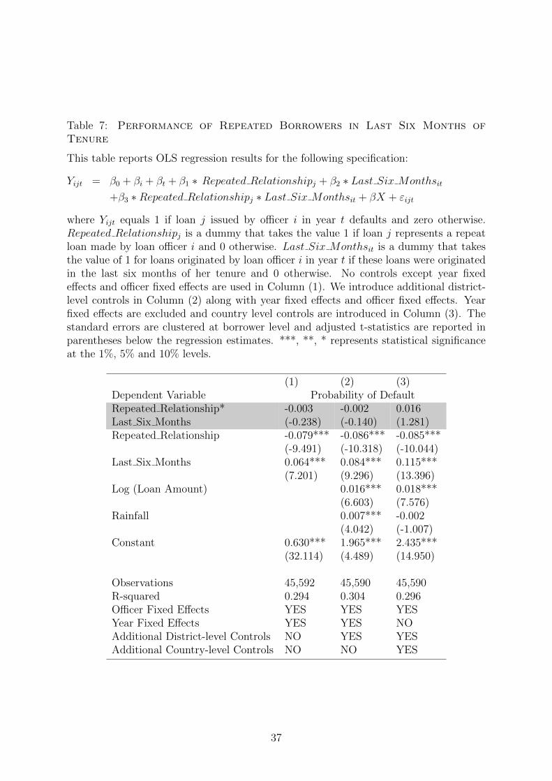
alternative thesis using the following specification:

Yijt = β0 + βi + βt + β1 ∗ Repeated Relationshipj + β2 ∗ Last Six Monthsit

+β3 ∗Repeated Relationshipj ∗ Last Six Monthsit + βX + εijt (19)

where Yijt equals 1 if loan j issued by officer i in year t defaults and zero otherwise.

Repeated Relationshipj is a dummy that takes the value 1 if loan j represents a repeat

loan made by loan officer i and 0 otherwise. Last Six Monthsit is defined as before.

In table 7, we report the results from testing equation (19). The specifications shown

in columns (1)-(3) of table 7 are similar to those in table 3 and in table 4. We observe that

the co-efficient estimate for β1 is negative and statistically significant in all specifications.

Thus, borrowers who share a repeated borrowing relationship with the departing loan

officer default less, which is consistent with relationship lending reducing the probability

of default (Puri, Rocholl, and Steffen, 2010). Because loans given out in the last six

months of the outgoing officer’s tenure are likely to be affected by job rotation, the

coefficient β2 captures the effect of job rotation for first-time borrowers:

β2 = (Y Loans issued in last 6 months − Y Loans issued earlier)∣∣first-time borrowers

For new borrowers, the loan officer has to make the effort to acquire soft information.

The positive and statistically significant coefficient estimate for β2 shows that job rota-

tion affects the effort by the loan officer to acquire soft information. Interestingly, the

coefficient estimate for the interaction term β3 is statistically indistinguishable from zero.

Because loans given out in the last six months of the outgoing officer’s tenure are likely

16It is possible that the new loan officer has formal or informal access to the old loan officer. In thiscontext, we note the following. First, based on our interviews with the bank officials and our reviewof official documents, we do not find any information suggesting that the current loan officer may haveformal access to the old loan officer. Second, the low powered incentives faced by loan officers in oursample make it less likely that that the new loan officer would informally access the old officer. Finally,such access between the old and new officers should serve to reduce the probability of default on loansaffected by job rotation, which would stack the odds against finding the positive effect of job rotation onthe probability of default. We therefore believe that the effect we obtain is robust to such access.

23

to be affected by job rotation, this evidence suggests that the above results are not driven

exclusively by repeat borrowers.

Overall, we conclude that the evidence presented in tables 4 to 7 is consistent with

our main thesis as predicted by proposition 2.

VI.E Effect Of Loan Officer Rotation On Loan Officer Effort

We now examine attempt to throw some light on this mechanism for the main effect.

We use the time elapsed between the date when a loan is repaid by the borrower and the

date when he gets a repeat loan. Any delay in renewing the loan can be a measure of

(lack of) effort by the loan officer. If it were the result of more careful consideration of the

loan application, we should see an improvement in loan performance due to job rotation.

In fact, we observe deterioration in loan performance due to job rotation. Therefore, a

delay in renewing the loan should proxy for lack of effort.

Of course, we only observe equilibrium outcomes for the number of days elapsed. It

is possible that farmers delay their current application because agricultural requirements

are seasonal in nature. For example, agricultural activity tends to be lowest during the

summer months of April and May. Hence, it is possible that a farmer who repays a

loan in March may wait till June before applying for his next loan. To control for such

seasonal effects, we can also include fixed effects for the month in which the repeat loan is

originated. These fixed effects enable us to control for unobserved differences in the days

elapsed depending on the month in which the repeat loan is originated. We therefore

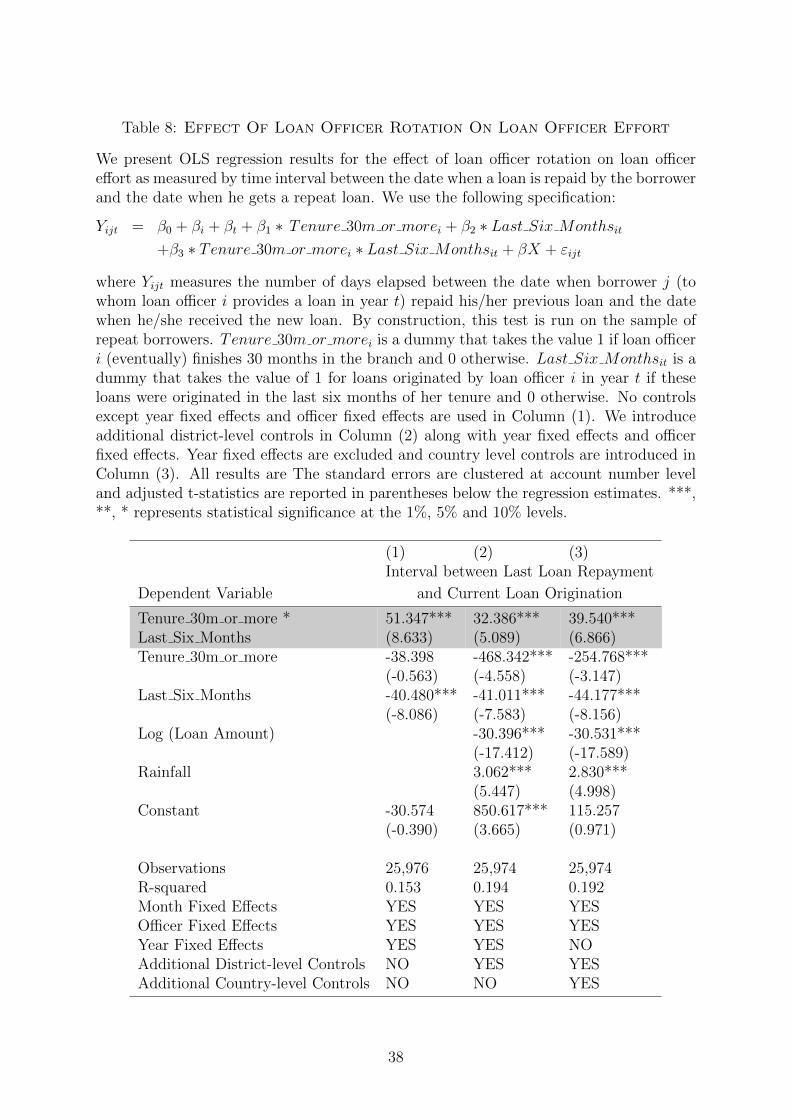
implement the following specification:

Yijt = β0 + βi + βt + βmonth + β1 ∗ Tenure 30m or morei + β2 ∗ Last Six Monthsit

+β3 ∗ Tenure 30m or morei ∗ Last Six Monthsit + βX + εijt (20)

where Yijt now measures the number of days elapsed between the date when borrower j

(to whom loan officer i provides a loan in year t) repaid his/her previous loan and the

date when he/she received the new loan. By construction, this test is run on the sample

of repeat borrowers. βmonth captures fixed effects for the month in which the new loan

was originated.

The results for this test are presented in table 8. Across columns (1)-(3), we find that

the coefficient estimate for β1 is negative and statistically significant except in column 1,

which suggests that loan officers that have a longer tenure in a branch take lesser time to

approve the loan for a repeat borrower. Similarly, we find that the coefficient estimate

for β2 is negative and statistically significant in each of the three columns, which suggests

that loan officers take lesser time to approve the loan for the repeated borrower in the

last six months of their tenure when compared to earlier periods. The negative coefficient

estimates for β1 and β2 suggests that the loan officer learns on the job and therefore takes

24

less time to approve the loan for a repeated borrower as his tenure in the branch increases.

However, crucially, we notice across columns 1 to 3 that the coefficient estimate for β3 is

positive and statistically significant. The economic effect is large as well: loans that are

affected by job rotation take between 32 to 51 days more for approval when compared to

loans that are not affected by job rotation, where the mean equals 10 days.

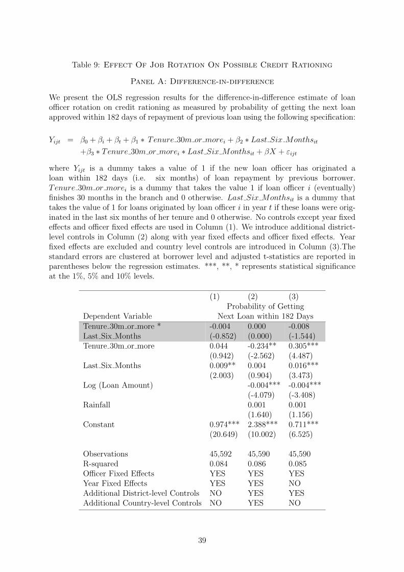
VI.F Effect Of Job Rotation On Possible Credit Rationing

We now test whether job rotation leads to possible credit rationing as implied by

Corollary 1, which implies that the incoming loan officer is likely to ration credit to

borrowers that had a borrowing relationship with the outgoing loan officer because of

lower effort exerted by the outgoing loan officer. We implement the following specification:

Yijt = β0 + βi + βt + β1 ∗ Tenure 30m or morei + β2 ∗ Last Six Monthsit

+β3 ∗ Tenure 30m or morei ∗ Last Six Monthsit + βX + εijt (21)

where Yijt is a dummy takes a value of 1 if the new loan officer has originated a loan within

182 days (i.e. six months) of loan repayment by previous borrower. Columns (1)-(3) in

Panel A of table 9 shows the results of these tests, where the specifications are similar

respectively to those in table 3 and in table 4. We notice that the coefficient estimate for β3

is statistically indistinguishable from zero, which suggests that the difference-in-difference

estimate for the effect of job rotation on a new loan being granted is insignificant. Thus,

the evidence does not seem to suggest overall credit rationing due to job rotation. We

therefore investigate if the new loan officer discriminates between borrowers handled by

the outgoing loan officer vis-a-vis other borrowers because the new loan officer may factor

in the possibility that the outgoing loan officer may not have invested optimal effort in

screening loans given out during the ending period of his tenure. We implement the

following specification:

Yijt = β0 + βi + βt + β1 ∗ Dummy loan officer changes after disbursementijt+β2 ∗Dummy loan officer changes after repaymentijt + βX + εijt (22)

where Yijt is a dummy takes a value of 1 if the new loan officer has originated a loan

within 182 (i.e. six months) days of loan repayment by previous borrower. Panel B shows

the results for testing equation (22). The specifications shown in columns (1)-(3) of Panel

B of table 9 are similar to those in table 3 and in table 4.

As evident from results in Panel B, columns (1)-(3), those borrowers that took a loan

during the tenure of the previous loan officer and subsequently the loan officer changed

before they repaid the loan have 9.6% less likelihood of getting a loan within 6 months

of their repayment. Interestingly, the succeeding loan officer is quite unlikely to lend

25

to those borrowers that received and repaid a loan in the last 6 months of the previous

loan officer’s tenure. They have a stark 63.5% lower likelihood of getting a loan within

next 6 months of their loan repayment. When the new loan officer provides a loan to

a borrower that got the loan during the tenure of the outgoing loan officer but repaid

during the new officer’s tenure, the new loan officer would have spent effort in monitoring

this borrower and collecting the dues from the borrower. The new loan officer would not

have however screened this borrower. In contrast, when the new loan officer provides a

loan to a borrower that got the loan and repaid the loan during the tenure of the outgoing

loan officer, the new loan officer has not spent effort on either screening this borrower

or in monitoring the borrower. The disproportionately larger effect for borrowers that

were screened and monitored by the outgoing loan officer when compared to the effect for

borrowers that were screened by the outgoing loan officer but were monitored by the new

loan officer is consistent with the predictions in Corollary 1. However, we don’t observe

overall credit rationing due to job rotation possibly because the new loan officer extends

loans to borrowers that were not handled by the outgoing loan officer.

VI.G Robustness

VI.G.1 Threshold Tenure for Classifying into Treatment and Control Groups

In table 10, we examine the robustness of our key by separating loan officers into the

treatment and control groups based on whether or not they have completed three years

in a particular branch. Because the expected tenure in a branch equals three years, a

loan officer that has already spent three years in a branch can be transferred at any point

in time. As a result, any loan that such a loan officer originates is likely to be monitored

and collected by his/her replacement. Therefore, loans that are originated by loan officers

that have spent three years in a branch are at least as likely to be affected by job rotation

as loans that originated by loan officers that have spent 2.5 years in a branch. For this

purpose, we employ the following specification:

Yijt = β0 + βi + βt + β1 ∗ Tenure 36m or morei + β2 ∗ Last Six Monthsit

+β3 ∗ Tenure 36m or morei ∗ Last Six Monthsit + βX + εijt (23)

where the only difference compared with (25) is the use of the Tenure 36m or morei

dummy instead of the Tenure 30m or morei dummy. To ensure that there is no other

change in our specification, we continue to compare the performance of loans originated

in the last six months of tenure vis-a-vis those originated earlier. Columns (1) and (2)

of table 10 show the results of testing using equation (23) . Column (1) shows the results

of the specification including year and officer fixed effects but without any other control

variables while column (2) shows the results of the specification including year and officer

26

fixed effects as well as other district level control variables. In both these columns, we

find that the results are as strong as before.

Next, to examine possible placebo effects that may be accounting for this result, we

examine whether the result is obtained when we separate loan officers into treatment and

control groups based on whether or not they have completed 1.5 years in a particular

branch. Because the expected tenure in a branch equals three years, a loan officer that

has only spent 1.5 years in a branch is unlikely to be transferred over the next 1.5 years.

As a result, the loan officer is likely to himself/herself monitor and collect any loan that

he/she originates in the next six months. Therefore, loans originated in the next six

months by loan officers that have only spent 1.5 years in a branch are unlikely to be

affected by job rotation. To test for this effect, we employ the following specification:

Yijt = β0 + βi + βt + β1 ∗ Tenure 18m or morei + β2 ∗ Last Six Monthsit

+β3 ∗ Tenure 18m or morei ∗ Last Six Monthsit + βX + εijt (24)

where the only difference compared with (25) is the use of the Tenure 18m or morei

dummy instead of the Tenure 30m or morei dummy. Here as well, we continue to com-

pare the performance of loans originated in the last six months of tenure vis-a-vis those

originated earlier. Columns (3) and (4) of table 10 show the results of testing using

equation (24) . while the coefficient estimate for β3 is negative and statistically significant

in column (3), it is insignificant in column (4). Thus, when we separate loan officers

into treatment and control groups based on a tenure of 18 months, we find that the

hypothesized effect of job rotation increasing the probability of default is not obtained.

These results Suggest that the above results for the effect of job rotation are not driven

by omitted variables that may be leading to some placebo effects.

VI.G.2 Time Varying Unobserved Officer Characteristics

Our causal claims are valid if there are no systematic differences in observable and

unobservable characteristics between the treatment and control group of loan officers.

Note that all our tests included loan officer fixed effects, which enabled us to control for

the effect of time-invarying characteristics of loan officers. However, time-varying loan

officer characteristics present a residual concern. Our empirical setting in a public sector

bank provides multiple lines of defence against such a concern. First, incentives in public

sector banks are low-powered. In particular, loan officers are promoted based on fixed

tenure in a particular role and not based on their performance in the role. So, time-

varying officer ability is unlikely to correlate with rotation on the job. Second, possible

confounding effects created by time-varying officer characteristics require the following

high hurdle. Difference in an unobserved characteristic of the treatment group of officers

in the last six months when compared to the same characteristic in the previous period

27

should be systematically different from the identical difference for the control group of

officers.

Nevertheless, we test for one possible source of time-varying unobserved officer charac-

teristics. It is possible that the control group of loan officers learn about their impending

transfer on promotion at least six months in advance and are thereby motivated to exert

more effort. If the same phenomenon manifests for the treatment group of officers as

well, then the systematic differences mentioned above would not result. Therefore, for

the confounding effects to materialise, lets presume that the above phenomenon affects

only the control group of officers and not the treatment group. This unlikely scenario

may produce results similar to what we have obtained so far. To rule out this possibility,

we rerun our basic difference-in-difference test as in equation (25) by excluding the four

officers who were transferred on promotion. The results for this test are displayed in

table 11. Our results are unchanged by this exclusion, which addresses concerns that our

results are confounded by such time-varying unobserved officer characteristics.

VII Conclusion

In this paper, we show that rotation of agents between tasks leads to costs that have

not yet been investigated in the literature. In particular, the costs we highlight stem

when decision-making inside a firm is driven by soft information because the principal

finds it difficult to fix sole responsibility when a task is underatken by multiple agents.

Our objective is to highlight a cost of job rotation that should be factored in when

analyzing the overall effect of job rotation. Because job rotation can alleviate agency

related problems relating to collusion, the ratchet effect, sub-optimal performance, etc.

we speculate based on the evidence in this paper that the net effect of job rotation may

be positive in organizational settings where hard information is relied upon for decision-

making. In contrast, the net effect may be negative in organizational settings where

soft information has to be relied upon for decision-making. A fruitful area for further

investigation would be to examine how the overall effect of job rotation varies with the

structure of information employed for decision-making in a firm.

References

Agarwal, S., and I. Ben-David (2014): “Do loan officers incentives lead to lax lendingstandards?,” Discussion paper, National Bureau of Economic Research.

Agarwal, S., and R. Hauswald (2010): “Authority and information,” in AFA 2011Denver Meetings Paper.

Aghion, P., and J. Tirole (1997): “Formal and real authority in organizations,”Journal of Political Economy, pp. 1–29.

28

Arya, A., and B. Mittendorf (2004): “Using job rotation to extract employee infor-mation,” Journal of Law, Economics, and Organization, 20(2), 400–414.

Banerjee, A., S. Cole, and E. Duflo (2008): “Are the monitors over-monitored:Evidence from Corruption, Vigilance, and Lending in Indian Banks,” Discussion paper,MIMEO, MIT.

Berg, T., M. Puri, and J. Rocholl (2013): “Loan officer incentives and the limitsof hard information,” Discussion paper, National Bureau of Economic Research.

Berger, A. N., N. H. Miller, M. A. Petersen, R. G. Rajan, and J. C. Stein(2005): “Does function follow organizational form? Evidence from the lending practicesof large and small banks,” Journal of Financial economics, 76(2), 237–269.

Berger, A. N., and G. F. Udell (2002): “Small business credit availability andrelationship lending: The importance of bank organisational structure,” The EconomicJournal, 112(477), F32–F53.

Burgess, R., and R. Pande (2003): “Do rural banks matter? Evidence from the In-dian social banking experiment,” Evidence from the Indian Social Banking Experiment(August 2003)., Vol.

Burgess, R., R. Pande, and G. Wong (2005): “Banking for the poor: Evidencefrom India,” Journal of the European Economic Association, 3(2-3), 268–278.

Cole, S. (2009): “Financial Development, Bank Ownership, and Growth: Or, DoesQuantity Imply Quality?,” The Review of Economics and Statistics, 91(1), 33–51.

Cole, S., M. Kanz, and L. Klapper (2013): “Incentivizing calculated risk-taking:evidence from an experiment with commercial bank loan officers,” Discussion paper,National Bureau of Economic Research.

DeYoung, R., D. Glennon, and P. Nigro (2008): “Borrower–lender distance, creditscoring, and loan performance: Evidence from informational-opaque small businessborrowers,” Journal of Financial Intermediation, 17(1), 113–143.

Di Maggio, M., and M. Van Alstyne (2012): “Information Sharing, Social Normsand Performance!,” .

Drexler, A., and A. Schoar (2011): “Does Soft Information Matters? EvidenceFrom Loan Officer Absenteeism,” Discussion paper, Working Paper, MIT Sloan Schoolof Management.

Fisman, R., D. Paravisini, and V. Vig (2012): “Cultural proximity and loan out-comes,” Discussion paper, National Bureau of Economic Research.

Hertzberg, A., J. Liberti, and D. Paravisini (2010): “Information and incentivesinside the firm: Evidence from loan officer rotation,” The Journal of Finance, 65(3),795–828.

Hirao, Y. (1993): “Task Assignmentand Agency Structures,” Journal of Economics &Management Strategy, 2(2), 299–323.

29

Holmstrom, B. (1982): “Moral hazard in teams,” The Bell Journal of Economics, pp.324–340.

Holmstrom, B., and P. Milgrom (1991): “Multitask principal-agent analyses: In-centive contracts, asset ownership, and job design,” JL Econ. & Org., 7, 24.

Khwaja, A. I., and A. Mian (2005): “Do lenders favor politically connected firms?Rent provision in an emerging financial market,” The Quarterly Journal of Economics,120(4), 1371–1411.

Liberti, J. M., and A. R. Mian (2009): “Estimating the effect of hierarchies oninformation use,” Review of financial studies, 22(10), 4057–4090.

Mahadevan, R., and S. Suardi (2013): “Is there a role for caste and religion in foodsecurity policy? A look at rural India,” Economic Modelling, 31, 58–69.

Mahul, O., and N. Verma (2012): “Improving farmers’ access to agricultural insur-ance in India,” World Bank Policy Research Working Paper, (5987).

Petersen, M. A. (2004): “Information: Hard and soft,” Discussion paper, workingpaper, Northwestern University.

Petersen, M. A., and R. G. Rajan (1995): “The effect of credit market competitionon lending relationships,” The Quarterly Journal of Economics, 110(2), 407–443.

(2002): “Does distance still matter? The information revolution in small busi-ness lending,” The Journal of Finance, 57(6), 2533–2570.

Puri, M., J. Rocholl, and S. Steffen (2010): “The impact of bank relationshipson default risk in consumer lending,” Available at SSRN 1572673.

Rajan, R. G. (1992): “Insiders and outsiders: The choice between informed and arm’s-length debt,” The Journal of Finance, 47(4), 1367–1400.

Ramakrishnan, R. T., and A. V. Thakor (1984): “Information reliability and atheory of financial intermediation,” The Review of Economic Studies, 51(3), 415–432.

Skrastins, J., and V. Vig (2013): “How Organizational Hierarchy Affects InformationProduction,” .

Stein, J. C. (2002): “Information production and capital allocation: Decentralizedversus hierarchical firms,” The Journal of Finance, 57(5), 1891–1921.

(2003): “Agency, information and corporate investment,” Handbook of the Eco-nomics of Finance, 1, 111–165.

Vig, V. (2013): “Access to collateral and corporate debt structure: Evidence from anatural experiment,” The Journal of Finance, 68(3), 881–928.

Visaria, S. (2009): “Legal reform and loan repayment: The microeconomic impact ofdebt recovery tribunals in India,” American Economic Journal: Applied Economics,pp. 59–81.

30

Table 1: Variable Description

The description of all the variables used in the regressions is provided below.

Variable DescriptionProbability of Default 1 when the loan has defaulted, 0 otherwiseLog (Loan Amount) Natural log of loan amount in rupeesLast Six Months Dummy variable; 1 when a loan is originated

in last 6 months of tenure of any loan officer,0 otherwise

Tenure 30m or more Dummy variable; 1 when a loan is origi-nated by a loan officer who has a tenure≥30 months, 0 otherwise

Default in Previous Loan Dummy variable; 1 when the borrower hasdefaulted in one’s previous loan, 0 otherwise

Interval between Loans Interval between last loan repayment andcurrent loan origination by the borrower indays

Next Loan within 182 Days Dummy variable; 1 when the next loan is is-sued within 182 days of repayment of previ-ous loan, 0 otherwise

Rainfall District-wise rainfall in cm in the year of loanorigination (Year)

Additional District-level Controls DescriptionDirect Agricultural Lending District-wise direct agricultural lending in

’000 crores in the year of loan origination(Year)

Indirect Agricultural Lending District-wise indirect agricultural lending in’000 crores in the year of loan origination(Year)

Total Deposit District-wise total bank deposit in ’000 croresin the year of loan origination (Year)

Literacy Rate District-wise literacy rate in percentage inthe year of loan origination (Year)

Inflation District-wise consumer price index in theyear of loan origination (Year)

Additional Country-level Controls DescriptionArea of Rice Production Area under rice crop production in ’0000

Hectares in the year of loan origination(Year)

Yield of Food Grains Kg/Hectares yield of all food grain in theyear of loan origination (Year)

Agricultural NPA Agricultural NPA in ’000 crores in the yearof loan origination (Year)

31

Tab

le2:

SummaryStatistics

Ou

rsa

mp

leco

mp

rise

of45

592

agri

cult

ura

lcr

oplo

ans

issu

edby

51lo

anoffi

cers

over

the

tim

ep

erio

dO

ctob

er2005

toM

ay2011.

Of

thes

e45592

loan

s,25

976

loan

sco

nst

itu

tere

pea

tlo

ans

wh

ile

the

rem

ain

ing

loan

sco

nst

itu

tefi

rst

tim

eb

orro

wer

s.

Var

iable

sN

o.of

Obs.

Mea

nM

edia

nSta

ndar

dD

evia

tion

Loa

nO

ffice

rT

enure

(Day

s)51

809.

1010

33.0

038

4.74

Pro

bab

ilit

yof

Def

ault

4559

20.

631.

000.

48In

terv

alb

etw

een

Curr

ent

and

Pre

vio

us

Loa

n(D

ays)

2597

650

.54

7.00

144.

76L

oan

Outs

tandin

g(D

ays)

4559

259

9.37

508.

0046

7.32

Fra

ctio

nof

Loa

ns

issu

edin

Las

t6

mon

ths

ofT

enure

4559

20.

300.

000.

46L

oan

Am

ount

(IN

R)

4559

059

456.

1130

000.

0015

1304

9.00

Rai

nfa

ll(c

m)

4559

210

.00

9.39

3.78

Are

aof

Ric

eP

roduct

ion

(’00

00H

ecta

res)

4559

235

57.6

539

78.0

011

52.5

2A

gric

ult

ura

lN

PA

(IN

Rbillion

s)45

592

95.4

71.5

43.5

Yie

ldof

Food

Gra

ins

(Kg/

Hec

tare

s)45

592

1803

.36

1798

.00

90.3

2D

irec

tA

gric

ult

ura

lL

endin

g(I

NR

billion

s)45

592

7429

.060

97.7

4664

.8In

dir

ect

Agr

icult

ura

lL

endin

g(I

NR

billion

s)45

592

855.

048

0.6

717.

1T

otal

Dep

osit

s(I

NR

billion

s)45

592

6987

7.0

6967

0.0

4402

4.0

Lit

erac

yR

ate

(in

per

centa

ge)

4559

255

.94

54.9

06.

33In

flat

ion

(Con

sum

erP

rice

Index

)45

592

145.

3613

4.75

26.9

8

32

Table 3: Effect of Loan Officer Rotation on Probability of Default

We present OLS regression results for the effect of loan officer rotation on the probabilityof default using the following specification:

Yijt = β0 + βi + βt + β1 ∗ Last Six Monthsit + βX + εijt

where Yijt equals 1 if loan j issued by officer i in year t defaults and zero otherwise. TheLast Six Monthsit is a dummy that takes the value of 1 for loans originated by loanofficer i in year t if these loans were originated in the last six months of her tenure and0 otherwise. No controls except year fixed effects and officer fixed effects are used inColumns (1). We introduce additional district-level controls in Column (2) along withyear fixed effects and officer fixed effects. Year fixed effects are excluded and country levelcontrols are introduced in Columns (3). The standard errors are clustered at borrowerlevel and adjusted t-statistics are reported in parentheses below the regression estimates.***, **, * represents statistical significance at the 1%, 5% and 10% levels.

(1) (2) (3)Dependent Variable Probability of Default

Last Six Months 0.057*** 0.075*** 0.113***(6.758) (8.795) (13.967)

Log (Loan Amount) 0.012*** 0.015***(4.678) (5.768)

Rainfall 0.008*** -0.000(4.730) (-0.095)

Constant 0.623*** 2.321*** 2.731***(31.259) (5.286) (17.265)

Observations 45,592 45,590 45,590R-squared 0.290 0.300 0.292Officer Fixed Effects YES YES YESYear Fixed Effects YES YES NOAdditional District-level Controls NO YES YESAdditional Country-level Controls NO NO YES

33

Table 4: Difference-in-difference Test for the Effect of Loan OfficerRotation on Probability of Default

We present OLS regression results for the difference-in-difference estimate of job rotationon probability of default using the following specification:

Yijt = β0 + βi + βt + β1 ∗ Tenure 30m or morei + β2 ∗ Last Six Monthsit

+β3 ∗ Tenure 30m or morei ∗ Last Six Monthsit + βX + εijt

where Yijt equals 1 if loan j issued by officer i in year t defaults and zero otherwise.Tenure 30m or morei is a dummy that takes the value 1 if loan officer i (eventually)finishes 30 months in the branch and 0 otherwise. Last Six Monthsit is a dummy thattakes the value of 1 for loans originated by loan officer i in year t if these loans wereoriginated in the last six months of her tenure and 0 otherwise. No controls except yearfixed effects and officer fixed effects are used in Column (1). We introduce additionaldistrict-level controls in Column (2) along with year fixed effects and officer fixed effects.Year fixed effects are excluded and country level controls are introduced in Column (3).The standard errors are clustered at borrower level and adjusted t-statistics are reportedin parentheses below the regression estimates. ***, **, * represents statistical significanceat the 1%, 5% and 10% levels.

(1) (2) (3)Dependent Variable Probability of Default

Tenure 30m or more * 0.075*** 0.048*** 0.107***Last Six Months (5.406) (3.490) (7.703)Tenure 30m or more -0.258*** -1.110*** -1.256***

(-2.931) (-4.510) (-9.193)Last Six Months -0.003 0.036*** 0.026**

(-0.228) (2.705) (2.020)Log (Loan Amount) 0.012*** 0.015***

(4.792) (6.067)Rainfall 0.008*** 0.001

(4.890) (0.441)Constant 0.885*** 3.445*** 4.141***

(9.794) (5.232) (17.074)

Observations 45,592 45,590 45,590R-squared 0.291 0.300 0.293Officer Fixed Effects YES YES YESYear Fixed Effects YES YES NOAdditional District-level Controls NO YES YESAdditional Country-level Controls NO NO YES

34

Tab

le5:

Sepa

rateEffectsofLoanOfficerRotationonTreatmentand

ControlGroups

We

rep

ort

OL

Ses

tim

ates

ofre

gres

sing

loan

def

ault

dum

my

onth

edum

my

forLastSixMonths

ofth

etr

eatm

ent

grou

p,

i.e.

loan

office

rsw

ho

hav

esp

ent

atle

ast

30m

onth

sin

apar

ticu

lar

bra

nch

,an

dth

eco

ntr

olgr

oup,

i.e.

loan

office

rsw

ho

hav

esp

ent

less

than

30m

onth

sin

apar

ticu

lar

bra

nch

.

Yijt

=β

0+βi+βt+β

1∗LastSixMonths i

t+βX

+ε i

jt

wher

eYijt

equal

s1

iflo

anj

issu

edby

office

ri

inye

art

def

ault

san

dze

root

her

wis

e.T

heLastSixMonths i

tis

adum

my

that

take

sth

eva

lue

of1

for

loan

sor

igin

ated

by

loan

office

ri

inye

art

ifth

ese

loan

sw

ere

orig

inat

edin

the

last

six

mon

ths

ofher

tenure

and

0ot

her

wis

e.N

oco

ntr

ols

exce

pt

year

fixed

effec

tsan

doffi

cer

fixed

effec

tsar

euse

din

Col

um

ns

(1)

and

(4).

We

intr

oduce

addit

ional

dis

tric

t-le

vel

contr

ols

inC

olum

ns

(2)

and

(5)

alon

gw

ith

year

fixed

effec

tsan

doffi

cer

fixed

effec

ts.

Yea

rfixed

effec

tsar

eex

cluded

and

countr

yle

vel

contr

ols

are

intr

oduce

din

Col

um

ns

(3)

and

(6)

ofP

anel

B.

The

stan

dar

der

rors

are

clust

ered

atb

orro

wer

leve

lan

dad

just

edt-

stat

isti

csar

ere

por

ted

inpar

enth

eses

bel

owth

ere

gres

sion

esti

mat

es.

***,

**,

*re

pre

sents

stat

isti

cal

sign

ifica

nce

atth

e1%

,5%

and

10%

leve

ls.

(1)

(2)

(3)

(4)

(5)

(6)

Dep

enden

tV

aria

ble

Pro

bab

ilit

yof

Def

ault

Tre

atm

ent

(Ten

ure

≥30

mon

ths)

Con

trol

(Ten

ure<

30m

onth

s)

Las

tSix

Mon

ths

0.06

4***

0.07

6***

0.12

6***

0.03

0-0

.137

***

-0.0

91**

*(6

.777

)(7

.746

)‘

(1.3

61)

(-6.

296)

(-4.

054)

Log

(Loa

nA

mou

nt)

0.00

6*0.

010*

**0.

029*

**0.

030*

**(1

.686

)(3

.010

)(6

.859

)(7

.134

)R

ainfa

ll0.

009*

**0.

001

0.01

8*0.

071*

**(4

.795

)(0

.456

)(1

.715

)(9

.822

)C

onst

ant

0.63

2***

3.92

1***

3.70

4***

0.66

7***

-12.

549*

**0.

509

(30.

952)

(5.6

65)

(14.

023)

(6.8

14)

(-7.

498)

(1.1

75)

Obse

rvat

ions

30,8

3330

,833

30,8

3314

,759

14,7

5714

,757

R-s

quar

ed0.

180

0.18

30.

174

0.49

20.

529

0.52

1O

ffice

rF

ixed

Eff

ects

YE

SY

ES

YE

SY

ES

YE

SY

ES

Yea

rF

ixed

Eff

ects

YE

SY

ES

NO

YE

SY

ES

NO

Addit

ional

Dis

tric

t-le

vel

Con

trol

sN

OY

ES

YE

SN

OY

ES

YE

SA

ddit

ional

Cou

ntr

y-l

evel

Con

trol

sN

ON

OY

ES

NO

NO

YE

S

35

Table 6: Disentangling Possible Effects of Hard Information

To test whether job rotation affects a verifiable measure of loan portfolio quality, we reportOLS regression results for the difference in difference estimate of loan officer rotation onthe credit worthiness of the loan portfolio, as measured by default in previous loan usingthe following specification:

Yijt = β0 + βi + βt + β1 ∗ Tenure 30m or morei + β2 ∗ Last Six Monthsit

+β3 ∗ Tenure 30m or morei ∗ Last Six Monthsit + βX + εijt

where Yijt equals 1 if borrower j (to whom loan officer i issued a loan in year t) hasdefaulted in the previous loan and 0 otherwise. Tenure 30m or morei is a dummy thattakes the value 1 if loan officer i (eventually) finishes 30 months in the branch and 0otherwise. Last Six Monthsit is a dummy that takes the value of 1 for loans originatedby loan officer i in year t if these loans were originated in the last six months of hertenure and 0 otherwise. No controls except year fixed effects and officer fixed effects areused in Column (1). In Column (2) we use log of the loan amount along with year andofficers fixed effects. We do not use any additional controls to avoid look ahead bias. Thestandard errors are clustered at borrower level and adjusted t-statistics are reported inparentheses below the regression estimates. ***, **, * represents statistical significanceat the 1%, 5% and 10% levels.

(1) (2)Dependent Variable Default in Previous Loan

Tenure 30m or more * 0.023 0.018Last Six Months (1.218) (0.950)Tenure 30m or more -0.014 -0.027

(-0.133) (-0.262)Last Six Months -0.057*** -0.056***

(-3.555) (-3.486)Log (Loan Amount) -0.018***

(-5.311)Constant -0.038 0.163

(-0.358) (1.436)

Observations 25,976 25,974R-squared 0.255 0.256Officer Fixed Effects YES YESYear Fixed Effects YES YES

36

Table 7: Performance of Repeated Borrowers in Last Six Months ofTenure

This table reports OLS regression results for the following specification:

Yijt = β0 + βi + βt + β1 ∗ Repeated Relationshipj + β2 ∗ Last Six Monthsit

+β3 ∗Repeated Relationshipj ∗ Last Six Monthsit + βX + εijt

where Yijt equals 1 if loan j issued by officer i in year t defaults and zero otherwise.Repeated Relationshipj is a dummy that takes the value 1 if loan j represents a repeatloan made by loan officer i and 0 otherwise. Last Six Monthsit is a dummy that takesthe value of 1 for loans originated by loan officer i in year t if these loans were originatedin the last six months of her tenure and 0 otherwise. No controls except year fixedeffects and officer fixed effects are used in Column (1). We introduce additional district-level controls in Column (2) along with year fixed effects and officer fixed effects. Yearfixed effects are excluded and country level controls are introduced in Column (3). Thestandard errors are clustered at borrower level and adjusted t-statistics are reported inparentheses below the regression estimates. ***, **, * represents statistical significanceat the 1%, 5% and 10% levels.

(1) (2) (3)Dependent Variable Probability of DefaultRepeated Relationship* -0.003 -0.002 0.016Last Six Months (-0.238) (-0.140) (1.281)Repeated Relationship -0.079*** -0.086*** -0.085***

(-9.491) (-10.318) (-10.044)Last Six Months 0.064*** 0.084*** 0.115***

(7.201) (9.296) (13.396)Log (Loan Amount) 0.016*** 0.018***

(6.603) (7.576)Rainfall 0.007*** -0.002

(4.042) (-1.007)Constant 0.630*** 1.965*** 2.435***

(32.114) (4.489) (14.950)

Observations 45,592 45,590 45,590R-squared 0.294 0.304 0.296Officer Fixed Effects YES YES YESYear Fixed Effects YES YES NOAdditional District-level Controls NO YES YESAdditional Country-level Controls NO NO YES

37

Table 8: Effect Of Loan Officer Rotation On Loan Officer Effort

We present OLS regression results for the effect of loan officer rotation on loan officereffort as measured by time interval between the date when a loan is repaid by the borrowerand the date when he gets a repeat loan. We use the following specification:

Yijt = β0 + βi + βt + β1 ∗ Tenure 30m or morei + β2 ∗ Last Six Monthsit

+β3 ∗ Tenure 30m or morei ∗ Last Six Monthsit + βX + εijt

where Yijt measures the number of days elapsed between the date when borrower j (towhom loan officer i provides a loan in year t) repaid his/her previous loan and the datewhen he/she received the new loan. By construction, this test is run on the sample ofrepeat borrowers. Tenure 30m or morei is a dummy that takes the value 1 if loan officeri (eventually) finishes 30 months in the branch and 0 otherwise. Last Six Monthsit is adummy that takes the value of 1 for loans originated by loan officer i in year t if theseloans were originated in the last six months of her tenure and 0 otherwise. No controlsexcept year fixed effects and officer fixed effects are used in Column (1). We introduceadditional district-level controls in Column (2) along with year fixed effects and officerfixed effects. Year fixed effects are excluded and country level controls are introduced inColumn (3). All results are The standard errors are clustered at account number leveland adjusted t-statistics are reported in parentheses below the regression estimates. ***,**, * represents statistical significance at the 1%, 5% and 10% levels.

(1) (2) (3)Interval between Last Loan Repayment

Dependent Variable and Current Loan Origination

Tenure 30m or more * 51.347*** 32.386*** 39.540***Last Six Months (8.633) (5.089) (6.866)Tenure 30m or more -38.398 -468.342*** -254.768***

(-0.563) (-4.558) (-3.147)Last Six Months -40.480*** -41.011*** -44.177***

(-8.086) (-7.583) (-8.156)Log (Loan Amount) -30.396*** -30.531***

(-17.412) (-17.589)Rainfall 3.062*** 2.830***

(5.447) (4.998)Constant -30.574 850.617*** 115.257

(-0.390) (3.665) (0.971)

Observations 25,976 25,974 25,974R-squared 0.153 0.194 0.192Month Fixed Effects YES YES YESOfficer Fixed Effects YES YES YESYear Fixed Effects YES YES NOAdditional District-level Controls NO YES YESAdditional Country-level Controls NO NO YES

38

Table 9: Effect Of Job Rotation On Possible Credit Rationing

Panel A: Difference-in-difference

We present the OLS regression results for the difference-in-difference estimate of loanofficer rotation on credit rationing as measured by probability of getting the next loanapproved within 182 days of repayment of previous loan using the following specification:

Yijt = β0 + βi + βt + β1 ∗ Tenure 30m or morei + β2 ∗ Last Six Monthsit

+β3 ∗ Tenure 30m or morei ∗ Last Six Monthsit + βX + εijt

where Yijt is a dummy takes a value of 1 if the new loan officer has originated aloan within 182 days (i.e. six months) of loan repayment by previous borrower.Tenure 30m or morei is a dummy that takes the value 1 if loan officer i (eventually)finishes 30 months in the branch and 0 otherwise. Last Six Monthsit is a dummy thattakes the value of 1 for loans originated by loan officer i in year t if these loans were orig-inated in the last six months of her tenure and 0 otherwise. No controls except year fixedeffects and officer fixed effects are used in Column (1). We introduce additional district-level controls in Column (2) along with year fixed effects and officer fixed effects. Yearfixed effects are excluded and country level controls are introduced in Column (3).Thestandard errors are clustered at borrower level and adjusted t-statistics are reported inparentheses below the regression estimates. ***, **, * represents statistical significanceat the 1%, 5% and 10% levels.

(1) (2) (3)Probability of Getting

Dependent Variable Next Loan within 182 DaysTenure 30m or more * -0.004 0.000 -0.008Last Six Months (-0.852) (0.000) (-1.544)Tenure 30m or more 0.044 -0.234** 0.305***

(0.942) (-2.562) (4.487)Last Six Months 0.009** 0.004 0.016***

(2.003) (0.904) (3.473)Log (Loan Amount) -0.004*** -0.004***

(-4.079) (-3.408)Rainfall 0.001 0.001

(1.640) (1.156)Constant 0.974*** 2.388*** 0.711***

(20.649) (10.002) (6.525)

Observations 45,592 45,590 45,590R-squared 0.084 0.086 0.085Officer Fixed Effects YES YES YESYear Fixed Effects YES YES NOAdditional District-level Controls NO YES YESAdditional Country-level Controls NO YES NO

39

Panel B: Discrimination Against Borrowers Handled by the OutgoingLoan Officer

In Panel B, we present OLS regression results for the effect of job rotation on the newloan officer discriminating between borrowers handled by the outgoing loan officer vis-a-vis other borrowers. We use the following specification:

Yijt = β0 + βi + βt + β1 ∗ Dummy loan officer changes after disbursementijt+β2 ∗Dummy loan officer changes after repaymentijt + βX + εijt

where Yijt is a dummy takes a value of 1 if the new loan officer has orig-inated a loan within 182 (i.e. six months) days of loan repayment bythe same borrower. Dummy loan officer changes after disbursementijt takes avalue of 1 if the outgoing loan officer changes after loan disbursement andDummy loan officer changes after repaymentijt takes a value of 1 if the outgoingloan officer changes after repayment. No controls except year fixed effects and officerfixed effects are used in Column (1). We introduce additional district-level controls inColumn (2) along with year fixed effects and officer fixed effects. Year fixed effects areexcluded and country level controls are introduced in Column (3). The standard errorsare clustered at borrower level and adjusted t-statistics are reported in parentheses belowthe regression estimates. ***, **, * represents statistical significance at the 1%, 5% and10% levels.

(1) (2) (3)Probability of Getting

Dependent Variable Next Loan within 182 DaysDummy for Loan Officer Changes -0.096*** -0.097*** -0.095***After Disbursement (-31.311) (-31.643) (-31.231)Dummy for Loan Officer Changes -0.635*** -0.637*** -0.636***After Repayment (-30.421) (-30.683) (-30.527)Log (Loan Amount) -0.004*** -0.003***

(-3.665) (-2.827)Rainfall 0.003*** 0.001*

(3.772) (1.693)Constant 1.037*** 2.146*** 0.875***

(124.379) (12.980) (16.341)

Observations 45,592 45,590 45,590R-squared 0.191 0.194 0.192Officer Fixed Effects YES YES YESYear Fixed Effects YES YES NOAdditional Controls NO YES YES

40

Table 10: Robustness of Difference-in-difference Result

We present robustness of the difference-in-difference estimate using two different cut-offsfor tenure to define treatment and control groups. The regression specification is similarto that employed in Table 4. In Columns (1) and (2), treatment and control groups arebased on whether or not loan officers have completed three years in a particular branch.In Columns (3) and (4), treatment and control groups are based on whether or not loanofficers have completed 1.5 years in a particular branch. No controls except year fixedeffects and officer fixed effects are used in Column (1) and (3). We introduce additionaldistrict-level controls in Column (2) and (4) along with year fixed effects and officer fixedeffects. The standard errors are clustered at each borrower level and adjusted t-statisticsare reported in parentheses below the regression estimates. ***, **, * represents statisticalsignificance at the 1%, 5% and 10% levels.

(1) (2) (3) (4)Dependent Variable Probability of Default

Tenure Cutoff Tenure Cutoffm=36 Months m=18 Months

Dummy for Loan Officer Tenure ≥ m months * 0.075*** 0.048*** -0.120*** 0.002Last Six Months (5.406) (3.490) (-3.968) (0.050)Dummy for Loan Officer Tenure ≥ m months -0.258*** -1.110*** -0.096** -1.081***

(-2.931) (-4.510) (-2.438) (-4.589)Last Six Months -0.003 0.036*** 0.169*** 0.074**

(-0.228) (2.705) (5.708) (2.460)ln loan 0.012*** 0.012***

(4.792) (4.670)Rainfall(D) 0.008*** 0.008***

(4.890) (4.714)Constant 0.885*** 3.445*** 0.719*** 3.402***

(9.794) (5.232) (18.358) (5.165)

Observations 45,592 45,590 45,592 45,590R-squared 0.291 0.300 0.291 0.300Officer Fixed Effects YES YES YES YESYear Fixed Effects YES YES YES YESAdditional District-Level Controls NO YES NO YES

41

Table 11: Effect of Loan Officer Rotation on Probability of Default af-ter Excluding Officers who are Transferred on Promotion

We present OLS regression results for the difference-in-difference estimate of job rotationon probability of default after excluding officers who are transferred on promotion. Theregression specification is similar to that employed in Table 4. No controls except yearfixed effects and officer fixed effects are used in Column (1). We introduce additionaldistrict-level controls in Column (2) along with year fixed effects and officer fixed effects.Year fixed effects are excluded and country level controls are introduced in Column (3).The standard errors are clustered at borrower level and adjusted t-statistics are reportedin parentheses below the regression estimates. ***, **, * represents statistical significanceat the 1%, 5% and 10% levels.

(1) (2) (3)Dependent Variable Probability of Default

Tenure 30m or more * 0.111*** 0.159*** 0.170***Last Six Months (6.927) (8.814) (10.846)Tenure 30m or more -0.200** 1.708*** -1.665***

(-2.252) (5.416) (-11.246)Last Six Months -0.050*** -0.085*** -0.047***

(-3.240) (-4.936) (-3.082)Log (Loan Amount) 0.008*** 0.011***

(3.022) (4.321)Rainfall 0.001 -0.002

(0.517) (-1.071)Constant 0.820*** -3.811*** 5.387***

(8.976) (-4.502) (19.573)

Observations 40,946 40,944 40,944R-squared 0.268 0.280 0.273Officer Fixed Effects YES YES YESYear Fixed Effects YES YES NOAdditional District-level Controls NO YES YESAdditional Country-level Controls NO NO YES

42

Figure 2: Kaplan-Meier survival curve with Loan Officer Tenure inMonths

Note: The graph shows Kaplan-Meier survival curve (also known as the Kaplan-Meier productlimit estimate) against loan officers tenure (in months). The discontinuity in the graph occursat 12th quarter which illustrates that the average loan officer gets transferred after 3 years.

Figure 3: Histogram of Loan Disbursal Density with Loan Officer Tenurein Months

Note: The graph shows loan disbursal density against loan officers tenure in months.

43

Appendix A - Proofs

Consider the following first-order conditions for efforts eS and eM :

p1 (eS, eM) =1

x(25)

p2 (eS, eM) =1

x(26)

Differentiating (25) and (26) with respect to x, we obtain:

p11 (eS, eM)deSdx

+ p12 (eS, eM)deMdx

+1

x2= 0 (27)

p21 (eS, eM)deSdx

+ p22 (eS, eM)deMdx

+1

x2= 0 (28)

Solving the above expressions, we obtain:

deSdx

=p12 − p22

x2 (p11p22 − p212)

> 0;deSdx

=p12 − p11

x2 (p11p22 − p212)

> 0 (29)

because p12 > 0, p11 < 0, p22 < 0 and p11p22−p212 > 0 from concavity of p. Now comparing

(7) with (12) and (13), because α < 1, it follows that(eJRS , eJRM

)<(eN−JRS , eN−JR

M

). Then,

using p1 > 0 and p2 > 0, it follows that p(eJRS , eJRM

)< p

(eN−JRS , eN−JR

M

). Moreover,

from (9) , we have dUI

dp= (1 − α) (wp − wd) > 0 because α < 1 and from (3) wp >

wd. Now, because p(eJRS , eJRM

)< p

(eN−JRS , eN−JR

M

), U I

(eJRS , eJRM

)< U I

(eN−JRS , eN−JR

M

).

Therefore, the likelihood that the IR constraint for the new officer would be satisfied islower under job rotation than under no job rotation, which leads to Corollary.3

44

Appendix B - Location of Bank Branches

S.no Name Of the Branch District State

1 Paloncha Kothagudem Andhra Pradesh2 Bhadrachalam Road Kothagudem Andhra Pradesh3 Mahabubnagar Mahabub Nagar Andhra Pradesh4 Sattupalli Khammam Andhra Pradesh5 VM Banjara Khammam Andhra Pradesh6 Zaheerabad Medak Andhra Pradesh7 Kohir Medak Andhra Pradesh8 Medak Medak Andhra Pradesh9 Peddapally Karim Nagar Andhra Pradesh10 Sindhanur Raichur Karnataka11 Gangavathi Koppal Karnataka12 Parbhani Parbhani Maharashtra13 Nanded Nanded Maharashtra14 Ramtirth Nanded Maharashtra

45