TDA Progress Report 42-108 February 15, 1992 Software-Engineering Process (SEPS) C. Y. Lin Information Systems Division T. Abdel-Hamid Naval Postgraduate School Monterey, California J. S. Sherif Simulation Model Software Product Assurance Section I I and California State University at Fullerton This article describes the Software-Engineering Process Simulation (SEPS) model developed at JPL. SEPS is a dynamic simulation model of the software project-development process. It uses the feedback principles of system dynamics to simulate the dynamic interactions among various software lifecycle development activities and management decision-making processes. The model is designed to be a planning tool to examine trade-offs of cost, schedule, and functionality, and to test the implications of different managerial policies on a project’s outcome. Further- more, SEPS will enable software managers to gain a better understanding of the dynamics of software project development and perform postmortem assessments. 1. Introduction The development and maintenance of software systems is a growing business; it has been estimated that U.S. expenditures for software development and maintenance were $70 billion [14]. This figure is projected to grow to more than $255 billion in 1995 [ll], which accounts for 90 percent of total system expenditures [19]. However, the growth of the software industry has its downside. The record indicates that the development of software systems has been plagued by cost overruns, late deliveries, and dis- satisfied customers [20,36,45,47,52]. These pervasive prob- lems continue despite the significant software-engineering advances that have been made since the 1970s. There is a growing realization that most of these advanced tech- nologies focus too much on solving the technical problems of software production and not enough on the managerial aspect of software project development [29,34,41]. In recent years, the management component has fi- nally gained recognition as an area that is at the core 165 https://ntrs.nasa.gov/search.jsp?R=19920015071 2018-06-27T15:53:48+00:00Z
Transcript
TDA Progress Report 42-108 February 15, 1992
Software-Engi neeri ng Process (SEPS)
C. Y. Lin Information Systems Division
T. Abdel-Hamid Naval Postgraduate School
Monterey, California
J. S. Sherif
Simulation Model
Software Product Assurance Section I
I and
California State University at Fullerton
This article describes the Software-Engineering Process Simulation (SEPS) model developed at JPL. SEPS is a dynamic simulation model of the software project-development process. It uses the feedback principles of system dynamics to simulate the dynamic interactions among various software lifecycle development activities and management decision-making processes. The model is designed to be a planning tool to examine trade-offs of cost, schedule, and functionality, and to test the implications of different managerial policies on a project’s outcome. Further- more, SEPS will enable software managers to gain a better understanding of the dynamics of software project development and perform postmortem assessments.
1. Introduction The development and maintenance of software systems
is a growing business; it has been estimated that U.S. expenditures for software development and maintenance were $70 billion [14]. This figure is projected to grow to more than $255 billion in 1995 [ll], which accounts for 90 percent of total system expenditures [19]. However, the growth of the software industry has its downside. The record indicates that the development of software systems has been plagued by cost overruns, late deliveries, and dis-
satisfied customers [20,36,45,47,52]. These pervasive prob- lems continue despite the significant software-engineering advances that have been made since the 1970s. There is a growing realization that most of these advanced tech- nologies focus too much on solving the technical problems of software production and not enough on the managerial aspect of software project development [29,34,41].
In recent years, the management component has fi- nally gained recognition as an area that is at the core
of both the problems, as well as the solutions for soft- ware crises [12,21,53]. For example, the defense-science board task-force investigation, led by Professor Frederick Brooks, concluded that the problems with military soft- ware development were not technical but managerial. The report urges not to apply technical fixes to what are man- agement problems [15]. Furthermore, Dr. Richard F. Mer- win, a guest editor for a special issue of IEEE Transactions on Software Engineering devoted to project management, pointed out that “Programming disciplines such as top- down design, use of standardized high-level programming languages, and program library support systems all con- tributed to production of reliable software on time, within budget . . . . What is still missing is the overall manage- ment fabric which allows the senior project manager to understand and lead major data processing development efforts.” [34] And lastly, Abdel-Hamid notes, “Recently, it has become more and more evident that in software, product innovation is no longer the primary bottleneck to progress. The bottleneck is project management innova- tion.” [3]
Thus, there is a growing belief that to minimize fail- ures, good software-engineering practices are essential, but at the same time, there is a strong need to improve and advance existing software-management technology. Con- sequently, this has motivated the authors to develop a new software management technology-the Software Engineer- ing and Management Process Simulation (SEPS) model, a software project-management tool.
The remainder of this section discusses software- management tools, the approaches used in existing tools, and a comparison of these tools with those of the SEPS model.
A. State of the Art
A number of different techniques and tools have been developed to aid software-development planning. There are cost-estimation and Critical Path Method/Program Evaluation and Review Techniques (CPM/PERT) models that support resource-management functions [9,13,42,49] and models for process-management functions [27,37,39, 541. Each of these models has strengths and limitations. The strength of process models and CPM systems is their ability to model in great detail the activities within the software-development process. Their weaknesses include the inability to account for managerial decision making (such as a preference to hire versus reschedule) and the lack of feedback, among activities, that underlie software- development dynamics.
Cost-estimation models produce initial estimates that are essential for project start-up planning. These cost models, nevertheless, are limited. Most are static models (cost parameters are time-independent) designed to pro- vide point estimates. They fail to capture management decision-making dynamics and their impact on project be- havior. Furthermore, they are not well suited for real-time estimation adjustments once a project starts.
In summary, the existing management tools tend to fo- cus on the software artifact and its transformation pro- cesses but fail to model the managerial and dynamic as- pects that are at the core of software project-development.
B. SEPS Ovenriew
SEPS is being developed to address the above weak- nesses, specifically, it integrates technological aspects of software production with the managerial aspects. SEPS was designed so that it could be used to conduct trade- offs (on an ongoing basis) with regard to project cost, schedule, and functionality, and also would allow manage- ment to evaluate the implications of different managerial policies on a project’s outcome. In addition, the authors sought to develop a model that would provide insight into the dynamics of the software-development process, since without a fundamental understanding of that process, the likelihood of any significant gains in software management is questionable [10,24,32].
To achieve that objective, the authors took a unique approach to developing SEPS that embodies: (1) dynamic feedback modeling, (2) an integrated view of the software project-development process, and (3) the use of simula- tion. The approach is articulated in more detail in [2]. The significance of these properties is summarized in the following paragraphs.
1. Dynamic Feedback Modeling. At the heart of the SEPS modeling task is the principle of dynamic feed- back. The advantage of using dynamic feedback was de- scribed by Ondash, Maloney, and Huerta [40]. “A unique feature of dynamic project models not offered by network- ing planning methodologies is the ability to calculate the ripple (secondary) effects on project cost and schedule due to changing requirements. These changes might include changing government regulations . . . [or] work force avail- ability. Ripple effects occur in labor productivity, unantic- ipated schedule slack and float time . . . . These processes can only be modeled by using dynamic modeling with ex- plicitly represented feedback mechanisms. In this respect, dynamic project models complement the static . . . mod-
166
els by providing the capability to readily perform sensitiv- ity analyses of likely perturbations and their consequential ripple effects.”
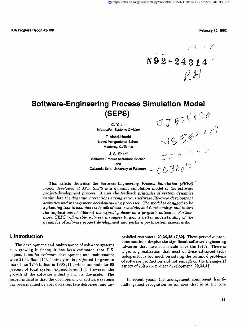
2. An Integrated View. Not only does SEPS en- capsulate and simulate the dynamic interactions among various software life-cycle engineering activities (e.g., de- sign, rework, inspection), but also it illustrates the influ- ential relationships among management functions (plan- ning, controlling, monitoring) and engineering activities (see Fig. 1). Only the integration of both engineering and management aspects allows one to examine the effective- ness of an intended management decision on overall project performance [2,31].
3. Simulation. Simulation is a powerful technique used to handle the complexity of the model (hundreds of dynamic variables and causal linkages). The use of sim- ulation enables managers to assess quickly and safely the implications of an intended policy before it is implemented. Also, users can easily conduct controlled postmortem ex- periments to develop new insights into .z project.
In summary, employing a feedback-modeling technique allows one to capture the dynamic ripple effect that char- acterizes software project development, and the integrated approach enforces an explicit description and enhances the understanding of the interrelationships among engineering activities and managerial decisions. Finally, the use of sim- ulation helps to reduce uncertainties and risks associated with a policy and provides support for ongoing project replanning.
Section I1 provides a summary of the process used to develop SEPS and its overall model structure. A detailed description of a submodel structure and some of its math- ematical formulations are also discussed.
II. SEPS Model Development The SEPS feedback structure was created by a rigor-
ous process that included three critical development steps: field interviews, literature review, and peer/expert review. The first step was to conduct a series of interviews with various software managers and engineers. Their views and hands-on experiences of how software systems are pro- duced were used to develop SEPS’s core feedback struc- ture. The information gathered included management and engineering practices, strategies, activity interactions, and the influential relationships among managerial decisions and development activities. After this information was in- corporated into the model structure, a literature review
was performed. The literature review provided the follow- ing benefits:
It verified the feedback structure by checking the structure obtained from field interviews with obser- vations from the open literature.
It supplemented knowledge in areas that are closely related to software development (such as manage- ment control, psychology, and organization behav- ior), and therefore enabled the authors to enhance the overall model structure [2].
At the end of the literature-review step, a fairly com- prehensive and integrated software project-development model was produced. This model was then subjected to iterative review and critique by experts (from JPL and other NASA centers) in the areas of modeling and simula- tion, software project management, and software engineer- ing. The review process produced a model structure that closely mimics the software project-development process.
The following sections present an overview of the SEPS model feedback structure. Included in the discussion are examples of mathematical formulations used in the model.
A. SEPS Structure Overview
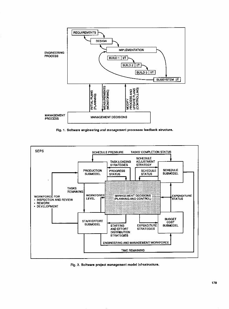
The SEPS model consists of the following four sub- models: Production, Staff/Effort, Scheduling, and Budget. Each submodel represents one part of the software project- development process and is linked to the others by a management-decision network. Together, these compo- nents represent an integrated view of the dynamics of the software project-development process. Figure 2 depicts a high-level view of the relationships among the four sub- models.
The Production submodel captures the various software production activities, their dependencies and interrelation- ships, and the functions that determine work progress. The Staff/Effort submodel simulates the functions that de- termine required work-force levels and mimics the flow of personnel resources. The Scheduling submodel encapsu- lates the functions that determine the time to complete a task and forecasts a completion time for each software life-cycle phase. The Budget submodel calculates expen- ditures and accumulated costs.
The decision-making characteristics in SEPS are de- rived from the dynamic feedback of information among the planning (e.g., for resources), monitoring (e.g., for prod- uct development), and controlling (e.g., the development process) functions. Also, since SEPS encompasses each
167
life-cycle phase, the structure shown in Fig. 2 exists within each phase.
Figure 3 illustrates a second level of abstraction for the interrelationships among the various components within each submodel. This figure shows how the submodels in- terrelate through a set of information-feedback links.
It is beyond the scope of this article to discuss in de- tail the entire SEPS model structure. Instead, the next section provides examples of the feedback structure of the variables included in the Production submodel and the relationships of these variables to other submodels. The relationships among variables are described by mathemat- ical formulations.
B. SEPS Feedback Structure: An Example The Production submodel starts with a number of tasks
(input parameter) to be developed. The number of tasks uncompleted is normally depleted through the software- production rate. However, as a project continues to de- velop, its scope is frequently altered. The changes can be attributed to various sources, such as the discovery of new tasks when requirements are better defined, or descoping tasks due to schedule or budget overruns. This relation- ship is illustrated in the upper left-hand quarter of Fig. 3.
Let W ( t ) denote the number of tasks to be developed at any time t (i.e., the backlog of work). Furthermore, let P(t - d t , t ) , R(t - d t , t ) and N(t - d t , t ) denote the team production rate (during time interval t - d t , t ) , task descoping rate, and new task discovery rate, respectively. There exists a relationship such that
W(1) = W(t - dt)
+ d t [ N ( t - d t , t ) - P(t - d t , t ) - R(t - d t , t ) ]
where dt is the time-increment interval. To simplify the discussion, the authors treat R(t - d t , t ) and N ( t - d t , t ) as exogenous variables that mimic management decisions based on information generated from other parts of the system (as shown in Fig. 3). These parameters can be ex- pressed as a pulse function or a time-tagged table function. The team production rate is defined as P(t - d t , t ) , which is a function of staff size, S(t); average productivity rate, Pa(t); intercommunication-overhead factor, C(t ) ; learning factor, L ( t ) ; and work-intensity factor, F ( t ) . The team production rate takes the form
where each Si(t) is the number of full-time equivalent staff of type i that is allocated for production at time t . In the model, staff is classified by their origins and experience levels. This results in four distinct groups of Si: in-house senior staff, in-house junior staff, newly hired senior staff, and newly hired junior staff. Si(t) is modeled in the Staff submodel as
+ d t [ A i ( t - d t , t ) - z ( t - d t , t ) - X i ( t - d t , t ) ]
(3)
where Ai( t -d t , t ) is the staff-assignment rate, z ( t - d t , t ) is the staff-release rate, and Xi( t - d t , t ) is staff-assimilation rate.
The weighted average productivity rate, Pa(t) is defined as
(4)
where each 8 is the nominal (unencumbered) individual staff-productivity rate for staff type i . Here the authors encapsulate within pi (a constant for each staff type) those productivity determinants cited by Boehm [13]. The rea- son for using static nominal productivity is based on the observation that even though productivity determinants vary from organization to organization, and from project to project within an organization, they remain constant within a single project [2].
There are three productivity determinants that exhibit dynamic characteristics during project development and, therefore, their effects on productivity are modeled explic- itly. The determinants are the intercommunication over- head factor, C(t ) ; the learning factor, L(t ) ; and the actual fraction of time an individual spends on a project, or work- intensity factor, F ( t ) .
The intercommunication overhead factor, C(t ) , is cited by many software researchers and practitioners as a signif- icant productivity determinant [2]. I t is generally agreed that increases in staff level for a project could have a neg- ative effect on team productivity [2,16,48,55]. The reason for this behavior is that adding staff to a project creates
168
additional communication overhead, such as verbal com- munication, documentation, and interfaces, all of which cause each team member’s productivity to drop below his or her normal rate. In Tausworthe’s work on intercommu- nication overhead [50], he points out that the team produc- tivity rate is affected by the intercommunication overhead factor, C(t), such that’
C(t) = [l - t(S)]
where t (S) is the relative productivity loss due to inter- communication among staff and is a function of staff size S. In the SEPS model, t (S) is derived from the data gath- ered from field interviews and the open literature [2], and it is defined as
t(s) = 1 - [1.03exp(-0.02~)]
and, therefore,
C(2) = 1.03exp(-O.O2S) ( 5 )
The learning factor, L ( t ) , can again be modeled by a time-tagged table function in which the independent vari- able is the percentage of work completed. The parametric value of L ( t ) shown in Fig. 5 has an S-shaped curve, as suggested by several authors [8,17,53].
Finally, the authors define F ( t ) as the work inten- sity, or the actual fraction of time an individual spends working on a project. In his doctoral work at the Mas- sachusetts Institute of Technology, Professor Abdel-Hamid conducted extensive research in this area. His review of the literature [4,5,6,25,30,33], combined with field interviews (5 organizations), led him to conclude that in the absence of schedule pressure, a person devotes, on average, 60 per- cent of his or her time working on project-related tasks. The remaining “slack time” is consumed by miscellaneous activities not directly related to the project, such as confer- ences, personal telephone calls, coffee breaks, and so on [2]. However, the effective work fraction fluctuates throughout a project. It would decrease even more if a project were ahead of schedule (negative schedule pressure), or increase, potentially up to 100 percent [13], if a project were behind schedule. Since it is known that F ( t ) can fluctuate dynam- ically throughout a project’s development, one can express it as a state variable
The authors took the liberty of changing Tausworthe’s notation so that it would be consistent with the notation used in this article.
or
where F ( 0 ) is the initial value of F ( t ) (e.g., 0.6), and T is the constant time required to realize the need to adjust work intensity. The desired fraction of daily work hours at time t is denoted by g ( t ) and is expressed as
where z( t ) is the fractional increase or decrease of effective work time, based on schedule pressure, from the initial fraction (Le., 0.6).
7 1:
Errors are made during the software development pro- cess; this characteristic is defined in SEPS as the error- generation rate. These human errors produce defects in products that remain undetected until product quality- assurance (QA) activities occur (e.g., formal inspections, design/code walk-throughs, and peer reviews). The QA effort will discover some defective products, but others will escape detection. These undetected faulty products will further affect the quality of subsequent products. This phenomenon is called the error-explosion factor. Let E(t - dt , t ) denote the error-generation rate, defined as
E(t - d t , t ) = [P(t - d t , t ) * N ( t ) * Y ( t ) * M(t)]
+ [P(t - d t , t ) * U ( t ) * 21 (7)
The first part of the right-hand side of Eq. (7) indicates that the defects are generated proportionally to the team production rate, P(t - d t , t ) . This is defined by the re- lationship between N ( t ) , the nominal number of defects committed per unit of work (e.g., source line of instruc- tion), and the dynamic factors Y ( t ) and M ( t ) , where Y ( t ) is the schedule pressure factor and M ( t ) is the work-force mix factor. N ( t ) can be modeled through a table func- tion in which the independent variable is the percentage of work completed for a given task, as shown in Fig. 6. The range of N ( t ) parameter values is based on the em- pirical evidence gathered by Boehm [13]; Jones [26]; and Thayer, Lipow, and Nelson [51]; however, these values are project dependent and can be calibrated accordingly. No- tice that N ( t ) is a nominal value, which means that a
169
certain number of errors will be created even though a project is right on track (e.g., no schedule slippage or un- planned workforce fluctuation). However, many software projects do experience some sort of schedule pressure (also known as schedule crunch) during their development life cycle. Schedule pressure has been found to cause an in- crease in the number of errors generated [1,4,5,35,43,44]. Hence, SEPS captures this phenomenon with variable Y ( t ) as the error-generation modifier due to schedule pressure,
l and its parametric value is shown in Fig. 7.
Finally, M ( t ) , the workforce-mix factor, is the last mod- ifier of the first part of the right-hand side of Eq. (7). When a project is facing a schedule crunch, management is often inclined to add staff to get the project back on track. Even though it would be desirable to add experienced in-house staff (e.g., a tiger team), these people may not be available. In such a case, management must find less-experienced in- house personnel or hire staff from outside the organiza- tion. In either approach, there would be an impact on both productivity and error generation (increase) [18,38]. SEPS introduces M ( t ) t o capture the dynamic changes in the workforce-mix ratio (e.g., experienced versus in- experienced staff) and its impact on the error-generation rate. The parametric value of M ( t ) is shown in Fig. 8 (derived from data gathered by Albrecht [5], Artzer, and Neidrauer [7]).
Thus far, error generation has been addressed with the assumption that the previous life-cycle-phase output prod- uct used to create the current-phase product is flawless. Of course, this is often not the case. One must therefore consider the existence of undiscovered defects from previ- ous life-cycle phases that create additional defects down- stream. The second part of the right-hand side of Eq. (7) is designed to model this characteristic. The behavior is modeled by saying that during production, additional de-
phase). The constant values of Z used in SEPS are based on the empirical study conducted by Kelly and Sherif [28]. In that study, the researchers found that the explosion fac- tor for developing ground software using Ada and/or C is about 15, from requirements analysis to coding. For flight software, the explosion factor from requirements analysis to coding is about 25.
Finally, a look at the error-detection rate completes the discussion of the Production submodel. As noted earlier, defective products remain undiscovered until QA activities occur. The causal loop structure for the error-detection rate, D(t ) , shown in Fig. 3, is illustrated in Fig. 4. Specifi- cally, the error-detection rate is a function of the product- inspection rate, I ( t - d t , t ) ; the error density, 6 ( t ) ; and the inspection efficiency factor, X ( t ) . This relationship is defined as
(9) D(t - d t , t ) = I ( t - d t , t ) * 6 ( t ) * X ( t )
and
-dW(t) I ( t - d t , t ) = -
dt
where W ( t ) denotes work units that have been developed and are ready for inspection, and
where P D indicates the level of potential detectable faulty products and is defined as
fects are created due to the density of previously unde- tected defects, U ( t ) , with an explosion factor, or latency, Z. U ( t ) is defined as
PD( t ) = PD(t - dt) -I- dt [E(t - d t , t , - - d t , t ) * 6(t)1 I
(12)
(8) (Undiscovered defects from previous phase)
J ( P ( t - dt , t )d t from previous phase U ( t ) =
and the latency factor 2 accounts for the fact that, for example, one design error will explode into five coding er- rors. Another way to express this behavior is that it will require more effort (often substantially more) to fix an er- ror that was not discovered in a previous phase. In SEPS, the 2’s are constants (since SEPS is a life-cycle model, 2 is allowed to have a distinct constant for each life-cycle
Empirical studies suggest that the effectiveness of detect- ing faulty products has a strong correlation to the level of QA effort allocated and the amount of products to be inspected in a given period of time (this correlation exists regardless of the QA technique used). The parametric val- ues used in SEPS to describe X ( t ) correspond with these studies and are shown in Fig. 9. The behavior exhibited in Fig. 9 indicates that the efficiency indicators correspond to the dependent variable J ( t ) , the units of work that are being inspected per staff hour (or week), as defined by
170
(9) Annual turnover rate.
where S,(t) is the actual level of staff allocated to QA, and is computed in the Effort/Staff submodel. Basically, Sq(t) is derived from the planned fraction of effort allocated for &A, a management-decision input parameter, with sched- ule pressure and training factors impacting the planned QA effort fraction.
So far, the SEPS model has been reviewed, and its de- velopment and feedback structure has been explained. In Section 111, the validity of SEPS is demonstrated by re- viewing its behavior when subjected to sensitivity analy- sis, and comparing it with the actual characteristics of a real project.
111. Validation of the SEPS Model A battery of validation tests designed to evaluate the
SEPS model is being carried out in two separate phases. Phase-1 validation tests were conducted in FY’91, and phase-2 validation tests will be performed during FY’92. Tests conducted in phase 1 included sensitivity analysis and historical project comparison. Sensitivity tests are used to check how sensitive the model is to perturba- tions over a range of input parameters, whereas historical project-comparison tests validate how precisely the model replicates historical projects. The results of phase-1 tests are presented in the following sections.
A. Sensitivity Analysis Tests
To conduct this test, the authors created a hypothetical software project where the project size is 128,000 source lines of code (sloc). The initial effort estimate was 1621 work-weeks with 95 weeks of project duration and an av- erage staff size of approximately 18 people.
Sensitivity analysis tests over nine SEPS input param- eters were performed. The input parameters are:
The graphical results of the sensitivity tests are shown in Figs. 10-18. The data were normalized for ease of demon- stration of the results. A brief description of each test follows
1. Staff Experience Level. A project normally con- sists of people with mixed experience levels; in this exper- iment the software engineers are grouped into two cate- gories: experienced and inexperienced staff. To demon- strate the effect of average team skill on the project (in terms of experience), the percentage of experienced staff level was varied from 30 to 100 percent, with 80 percent as the base case. The results indicate that as the fraction of experienced staff increases, the total effort and completion time required to complete the project decreases; however, the impact on project completion time is less significant than it is on effort. This is due to the management pres- sure to finish the project on schedule. (See Fig. 10.)
2. Project Size. It is well publicized that there is a strong correlation between the size of a software project and the effort and schedule needed to complete a project. In this experiment the authors verified whether SEPS can produce such behavior by varying the project size from 76.8 ksloc to 192 with 128 ksloc, as the base case. The results show that as the project site increases, both the total effort and completion time increase. (See Fig. 11.)
3. Initial Estimated Schedule (Compression/ Relaxation). Studies have demonstrated that the sched- ule estimated at the beginning of a project has a profound impact on the project’s outcome. To investigate the ef- fect the authors gradually compressed the initial estimated schedule from the base case (95 weeks) down to 60 percent (58 weeks) and also relaxed it to 150 percent (142 weeks). The results show that as the initial estimated schedule is compressed, the total effort required increases and, on the other hand, as the estimated schedule is extended, the total effort required decreases slightly. (See Fig. 12.)
4. Quality Assurance (QA) Effort. In this ex- periment the authors studied the effect of the percentage of total effort allocated to the software QA activities on project outcomes. The percentage of the QA effort was varied from 5 percent to 45 percent, with 15 percent as the base case, and the results show that both total effort and completion time increase if the planned quality assur- ance effort is either too high or too low. (See Fig. 13.)
5. Initial Staff Size. The initial staff size is defined in this experiment as the number of people assigned at the
171
beginning of a project. By using the Constructive Cost Model (COCOMO) [ll], an average staff size of 8 and peak staff size of 10 were obtained for the requirements- analysis phase. The authors started the experiment with 2 people and gradually increased the number to 10, with 8 as the base case. The results indicate that as the ini- tial requirements staff size is increased (up t o the planned peak value for the requirements phase), both total effort and completion time decrease. (Keep in mind that the authors assume that the staff will continue to participate throughout project life-cycle development; see Fig. 14.)
6. Staff Size Limit. The workforce limit is defined as the maximum allowable peak staff size during project development. In this experiment, the authors first ran the model without a workforce cap. As a result, the staff level peaked at 25. Next, the authors varied the workforce limit from 10 to 25, with 20 as the base case. The experiment results demonstrate that as the staff size limit is decreased (due to a hiring freeze, for example), the project comple- tion time is increased and the total effort is decreased; however, the drop in total effort is not significant. (See Fig. 15.)
7. Initial Estimated Effort. The initial estimated effort is defined as the total effort, estimated at the be- ginning of the project, required for developing a project. In this study the authors examined the effect of the initial estimated effort variation on the project’s final total effort and completion time. The results show that the project’s final total effort increases when the initial estimated effort is either severely underestimated or overestimated. The completion time tends to decrease as the initial estimated effort increases. (See Fig. 16.)
8. Error-Generation Rate. As explained in Sec- tion 11, during the product-development phase, it is almost certain that errors will be generated. In this experiment certain error rates are assumed and their effects on the project outcome is examined. When the error rates were varied from 2 to 40, with 10 (errors per ksloc) as the base case, the results show that the higher the error generation rate is, the higher the total effort and the longer the com- pletion t ime. It is assumed that the planned allocated Q A effort is a fixed function. (See Fig. 17.)
9. Annual Turnover Rate. It is a management nightmare to be confronted with a large staff-turnover rate. In this study the impact of varying staff annual turnover on project total effort and completion time is examined. The results show that a moderate increase in annual turnover rate causes an increase in completion time and no visible
variation in total effort . A higher turnover rate causes both the total effort and completion time to increase. (See Fig. 18.)
B. Evaluation of Sensitivity-Analysis Tests
Sensitivity analysis involves determining how much the simulation output will vary with a small change in an in- put parameter. It is a tool used to characterize the unique features of the original model. In general, sensitivity anal- ysis has four main uses: (1) assessing and interpreting the reasonableness of simulation, (2) experimental explo- ration of the model, (3) better allocation of resources for further data collection, and (4) promoting model simplifi- cation [46].
To evaluate the sensitivity-analysis tests, the authors relied on the experience of project managers and researchers at JPL and Goddard Space Flight Center (GSFC). Twenty-three staff members with an average of more than fifteen years experience in software man- agement and/or costing evaluated the sensitivity-analysis tests. Their assessments of the comparative accuracy of the model output to real life are summarized in Table 1.
The stratified survey of 23 experienced managers and researchers a t JPL and GSFC rated the behavior of the simulation model as reasonable 88 percent of the time, with a standard deviation of 0.02. A 95-percent confi- dence interval for the overall evaluation extends from 84 to 92 percent.
C. Historical Project Comparison
The sensitivity test is very effective in revealing abnor- malities in the model-generated behavior, which in turn indicate possible problems with the model structure or mathematical equations. In essence, this test examines a model’s correctness. However, the test does not confirm a model’s accuracy in prediction. Another test was there- fore conducted-a historical project case comparison-to validate the SEPS prediction capability.
The Cosmic Background Explorer (COBE) Attitude Ground Support System (AGSS) project at GSFC was chosen for the study as it maintained a detailed database and a well-documented report that describes the project- development history. The COBE/AGSS system was de- signed and implemented to support the COBE spacecraft mission, which began in July 1986 and was completed in August 1988. Its functional requirements include [23]:
(1) Provide ground-attitude determination.
172
1
(2) Monitor and verify attitude-control system (ACS)
(3) Provide attitude-sensor alignment and calibration.
(4) Provide spacecraft attitude-control support.
( 5 ) Provide ACS prediction support.
(6) Provide testing and simulation support.
(7) Provide contact prediction support.
performance.
The project characteristics are summarized as follows (see [23] for a detailed description of the project):
(1) Estimated size: 94.1 ksloc; actual size: 163.2 ksloc.
(3) Estimated duration: 85 staff weeks; actual duration:
(4) Language used: mostly Fortran, some Assembler.
( 5 ) Incremental development process used: three imple-
(6) Computer Science Corporation (CSC) was the con-
(7) Project started in July 1986 and ended in August
110 staff weeks.
mentation builds and two releases.
tracting developer.
1988.
The COBE/AGSS life-cycle phases modeled by SEPS in c 1 u d e :
Requirements analysis.
Preliminary design.
Detailed design.
Implement at ion :
(a) Three developmental builds.
(b) Three build integration/tests.
System test.
There are approximately twenty other parameters (e.g., hiring delay, nominal staff productivity, nominal staff at- trition) that are calibrated to the COBE/AGSS develop ment environment.
The validation scheme is presented in Fig. 19. The SEPS-predicted versus COBEactual project life-cycle staffing curve over time is shown in Fig. 20. The root mean squared error (RMSE) as a measure of accuracy between the predicted values of SEPS and actual values of COBE is 1.77 persons. Analysis of variance shows that on the av- erage there is no significant difference between the values predicted by SEPS and actual project life-cycle staffing values of COBE at the level of significance of Q = 0.01. Figure 21 illustrates a comparison of the accumulated ef- fort predicted by SEPS versus actual accumulated effort as a function of time. The RMSE measure of accuracy between the predicted values of SEPS and actual values of COBE is 13.6 person weeks. Analysis of variance shows that on the average there is no significant difference be- tween the values predicted by SEPS and COBE’s actual project-accumulated effort at the level of significance of a = 0.01. Finally, the schedule comparisons for each life- cycle phase are given in Fig. 22. The RMSE measure of accuracy between the values predicted by SEPS and the actual values of COBE is 2 weeks. Analysis of variance shows that on the average there is no significant difference between the values predicted by SEPS and COBE’s ac- tual project schedule end date at the level of significance of a = 0.01.
IV. Conclusions The increasing awareness of the need to improve the
quality of managerial software motivates the software in- dustry to come up with better management techniques and tools.
This article briefly reviewed some existing tools and then focused on the SEPS model. SEPS was developed to support software project planning and prevent software
The initial COBE/AGSS project estimates used as in- project-development failures. The specific objectives of SEPS are to assist software managers in preproject con- put parameters to SEPS include: tingency analyses and support project replanning (of cost and schedule, for example) during the development life cycle. In addition, SEPS provides a learning environment through simulation where the implications of different poli- cies on a project can be studied, and insight can be gained into the causes of project dynamics.
Initial project size (94.1 ksloc).
Initial project effort (241 staff months).
Planned life-cycle effort distribution [22].
Initial schedule estimates for the life cycle modeled.
Project-size growth estimate.
Nominal error-generation rate. Although more testing needs to be conducted, the find-
ings from the sensitivity test-with a confidence rating of
173
88 percent from the evaluators, and the results from the COBE historical project comparison at the level of signifi- cance a = 0.01-give the researchers and evaluators great confidence in the validity of the SEPS model.
SEPS has demonstrated its ability to replicate the soft- ware project dynamics observed in the software industry, and a specific project at GSFC, the next challenge for SEPS is to validate its applicability to the DSN.
References
[l] T. K. Abdel-Hamid, “On the Utility of Historical Project Statistics for Cost and Schedule Estimation,” Journal of Systems and Software, vol. 13, pp. 71-82, 1990.
[2] T. K. Abdel-Hamid, Software Project Dynamics: A n Integrated Approach, En- glewood Cliffs, New Jersey: Prentice-Hall, 1991.
[3] T. K. Abdel-Hamid, “Organizational Learning-The Key to Software Manage- ment Innovation,” American Programmer, vol. 4, no. 6, pp. 20-27, June 1991.
[4] D. S. Alberts, “The Economics of Software Quality Assurance,” Proceedings of the National Computer Conference, Montvale, New Jersey, pp. 433442, 1976.
[5] A. J . Albrecht, “Measuring Application Development Productivity,” Proceedings of the Joint SHARE/GUIDE/IBM Application Development Symposium, New York, pp. 83-92, October 1979.
[6] R. N. Anthony, Planning and Control Systems: A Framework for Analysis, Cam- bridge, Massachusetts: Harvard University Press, 1979.
[7] S. P. Artzer and R. A. Neidrauer, “Software Engineering Basics: A Primer for the Project Manager,” Unpublished thesis, Naval Postgraduate School, Monterey, California, 1982.
[8] J . M. Buxton, P. Naur, and B. Randell, eds., Software Engineering: Concepts and Techniques, New York: Litton Educational Publishing, Inc., 1976.
[9] J . W. Bailey and V. R. Basili, “A Meta-Model for Software Development Re- source Expenditures,” Proceedings of the 5th International Conference on Soft- ware Engineering, IEEE/ACM/NBS, New York, pp. 107-116, March 1981.
[lo] V. R. Basili, Tutorial on Models and Metrics for Software Management and Engineering, New York: Computer Society Press, 1980.
[ll] B. W. Boehm, “Improving Software Productivity,” Computer, vol. 20, pp. 43-50, September 1987.
[I21 B. W. Boehm, Software Risk Management, New York: IEEE Computer Society,
[13] B. W. Boehm, Software Engineering Economics, Englewood Cliffs, New Jersey: Prentice-Hall, 1981.
[14] B. W. Boehm and P. N. Papaccio, “Understanding and Controlling Software Costs,” IEEE Transactions on Software Engineering, vol. 14, no. 10, pp. 1462- 1477, October 1988.
1989.
[15] F. P. Brooks, Jr., “IEEE Software,” Softnews, vol. 13, p. 87, January 1988.
[16] F. P. Brooks, Jr., The Mythical Man-Month, Reading, Massachusetts: Addison- Wesley Publishing Co., 1978.
174
[17] J . Cooper, “Software Development Management Planning,” IEEE Dansactions
[18] A. G. Endres, “An Analysis of Errors and Their Causes in System Programs,’’
[19] R. E. Fairley, Software Engineering Concepts, New York: McGraw-Hill Book Co.,
[20] W. L. Frank, Critical Issues in Software: A Guide to Software Economics, Strat- egy , and Profitability, New York: John Wiley and Sons, 1983.
[21] P. F. Gehring, Jr . and V. W. Poovch, “Software Development Management,” Data Management, vol. 8, pp. 14-38, February 1977.
[22] Manager’s Handbook for Software Development, Revision I, Goddard Space Flight Center, Baltimore, Maryland, November 1990.
[23] Software Development History for Cosmic Background Explorer (COBE) Atti- tude Ground Support System (AGSS), Goddard Space Flight Center, Baltimore, Maryland, December 1988.
[24] W. S. Humphrey, Managing the Software Process, Reading, Massachusetts: Addison-Wesley Publishing Company, 1989.
[25] R. L. Ibrahim, “Software Development Information System,” Journal of Systems Management, vol. 11, pp. 34-39, December 1978.
[26] T . C. Jones, “Measuring Programming Quality and Productivity,” IBM Systems Journal, vol. 17, no. 1, pp. 39-63, 1978.
[27] M. Keller and M. Wilkins, “On the Use of an Extended Relational Model to Handle Changing Incomplete Information,” IEEE Tbansactions on Software En- gineering, vol. 11, no. 12, pp. 620-633, 1985.
[28] J . Kelly and Y . S. Sherif, “Where Is The Most Critical Point to Emphasize Software Inspections?,’’ IEEE Dansactions on Software Engineering, submitted in 1991.
[29] K. Kolence, “Software Engineering Management and Methodology,” Software Engineering: Report on a Conference Sponsored by the NATO Science Commit- tee , edited by P. Naur and R. Randell, New York: IEEE Press, vol. 13, pp. 116- 123, October 1968.
[30] J . H . Lehman, “HOW Software Projects Are Really Managed,” Datamation,
[31] C. Y. Lin and R. Levary, “Computer-Aided Software Process Design,” IEEE Transactions on Software Engineering, vol. 15, no. 9, pp. 1025-1037, September 1989.
[32] L. Liu and E. Horowitz, “A Formal Model for Software Project Management,” IEEE Dansactions on Software Engineering, vol. 15, no. 10, pp. 1280-1293, October 1989.
on Software Engineering, vol. 10, pp. 22-26, 1984.
IEEE Dansactions on Software Engineering, vol. 1, pp. 140-149, June 1975.
1985.
V O ~ . 25, pp. 35-41, 1979.
[33] C. L. McGowan and R. C. Henry, “Software Management” in Research Directions in Software Technology, edited by P. Wegner, Cambridge, Massachusetts: MIT Press, 1979.
[34] R. E. Merwin, “Software Management: We Must Find a Way,” IEEE Dansac- tions in Software Engineering, no. 4, pp. 307-361, 1978.
175
[35] H. D. Mills, Software Productivity, Toronto, Canada: Litter, Brown & Co., 1983.
[36] S. N. Mohanty, “Software Cost Estimation: Present and Future,” Software-
[37] P. Montgomery, Jr., “A Model of the Software Development Process,” Journal
[38] C. J . Myers, Software Reliability: Principles and Practices, New York: John Wiley
[39] M. Newman and R. Sabherwal, “A Process Model for the Control of Information System Projects,” Proceedings of the Tenth International Conference on Infor- mation Systems, New York, pp. 185-197, December 1989.
[40] S. C. Ondash, S. Maloney, and J . Huerta, “Large Project Simulation: A Power Tool for Project Management Analysis,” Proceedings of the 1988 Winter Simu- lation Conference, Los Angeles, pp. 231-239, January 1988.
Practice and Ezperience, vol. 11, pp. 103-121, 1981.
of Systems and Software, vol. 2, pp. 237-255, 1981.
and Sons, 1976.
[41] A. J . Perlis, “Software Engineering Education,” Software Engineering Tech- niques: Report on a Conference Sponsored b y the Nate Science Committee, edited by J . N. Baxton and B. Randell, October 1969.
[42] L. H. Putnam, “A General Empirical Solution to the Macro Software Sizing and Estimating Problem,” IEEE Transactions on Software Engineering, vol. 4,
[43] L. H. Putnam and A. Fitzsimmons, “Estimating Software Costs, Part I,” Data-
[44] A. Radice, “Productivity Measures in Software,” The Economics of Information Processing Vol. 2: Operations, Programming, and Software Models, edited by R. Goldberg and H . Lorin, New York: John Wiley and Sons, 1982.
[45] C. V. Ramamoorthy, K. H. Kim, and W. T . Chen, “Optional Placement of Software Monitors Aiding Systematic Testing,” IEEE Transactions on Software Engineering, vol. 1, pp. 46-58, 1975.
[46] M. R. Rose and R. Harmsen, “Using Sensitivity Analysis to Simplify Ecosystem
[47] B. R. Schlender, “How to Break the Software Logjam,” Fortune, vol. 212,
[48] R. F. Scott and D. B. Simmons, “Predicting Programming Productivity-A Communications Model,” IEEE Bansactions on Software Engineering, vol. 1, pp. 230-238, December 1975.
[49] R. C. Tausworthe, Deep Space Network Software Cost Estimation Model, JPL
[50] R. C. Tausworthe, “Staffing Implication of Software Productivity Models,” T D A Progress Report 42-72, vol. October-December, Jet Propulsion Laboratory, Pasadena, California, pp. 70-75, February 15, 1983.
Project Reality, New York: North Holland, 1978.
pp. 345-361, July 1978.
mation, vol. 25, pp. 189-198, September 1979.
Models: A Case Study,” Simulation, vol. 31, no. 1, pp. 15-24, 1978.
[51] T. A. Thayer, M. Lipow, and E. C. Nelson, Software Reliability: A Study of Large
[52] R. W. Thayer, A. Pyster, and R. Wood, “Major Issues in Software Engineering Project Management,” IEEE Bansactions on Software Engineering, vol. SE-7, no. 4, pp. 111-125, July 1981.
1 76 I I
[53] R. D. H. Warburton, “Managing and Predicting the Costs of Real-Time Soft-
[54] L. G . Williams, “Software Process Modeling: A Behavioral Approach,” IEEE
[55] M. V. Zelkowitz, “Perspectives on Software Engineering,” Computing Surveys,
ware,” IEEE lhnsac t ions in Soflware Engineering, vol. 9, pp. 502-509, 1983.
lhnsac t ions on Soflware Engineering, vol. 4 , pp. 174-186, 1978.
vol. 10, no. 2, pp. 197-216, June 1978.
Table 1. Staff members' evaluations of sensitivity-analysis tests.
Overall evaluation of sensitivity test StafT member
Standard deviations Reasonable = 1. Not reasonable = 0 Number Category
18 Manager 0.89 0.06 5 Researcher 0.87 0.18
23 Stratified 0.88 0.02
178
PROCESS MANAGEMENT I MANbGEMENT DECISIONS
Fig. 1. Software engineering and management processes feedback structure.
SEPS SCHEDULE PRESSURE TASKS COMPLETION STATUS
PRODUCTION
EXPENDITURE
DEVELOPMENT
I I ANUH-~WII t DISTRIBUTION STRATEGIES
ENGINEERING AND MANAGEMENT WORKFORCE I I I TIME REMAINING
Fig. 2. Sottware project management model infrastructure.
179
I- E 9 z 5 Q
W
n " Y v) 4 I-
S3IC331WlS DNlavOl SXSVl
I z
I I I I I I I I I I I I I I $ I : 1 ; I : : l g l a
m
180
f DISCZZED DEFECT- 4,->
ERROR TASKS TO )C INSP~CTION e INS~ECTION DENSITY\ BE INSPECTED d RATE y EFFECTIVENESS
UNDETECTED
PRODUCTS I I
PLANNED SCHEDULE QUALITY- PRESSURE
EFFORT
t ERROR-
GENERATION ASSURANCE RATE
Fig. 4. Error-detection-rate submodel.
- 0 0.2 0.4 0.6 0.8 1.0
PERCENT OF TASK WORKED
Fig. 5. Learning factor on potential productivity rate.
40
0- W I- & 30- I
W
6 10- m I 3 z
DESIGN- CODING
I s 0 7 I I I I I + 0 0.2 0.4 0.6 0.8 1 .o
DESIGN- CODING
I I I I I + 0 0.2 0.4 0.6 0.8 1 .o
PERCENT OF TASK WORKED
Fig. 6. Nominal errors generated per ksloc.
EFFORT NEEDED - EFFORT REMAINING EFFORT REMAINING
I I I I I I I .4 -0.2 0 0.2 0.4 0.6 0.8 1.0
SCHEDULE PRESSURE
Fig. 7. Schedule pressure factor on error-generation rate.
181
1.3
PERCENT OF STAFF THAT IS EXPERIENCED
Fig. 8. Staff-mix effect on error-generation rate.
21 I- rn
20
19 0
8 17 v)
16 0 8 15 w
a
f 18
w 14 13
g! 12 a
11
10 9
I I I I
INSPECTION RATE, source staternenvhr 70 TO 122 130 TO 285
Fig. 9. Error-detection rate.
s 1.0 COMPLETION TIME (weeks)
0.9 1 \
0.8 4 30 40 50 60 70 80 90 1c
EXPERIENCED STAFF, percent
Fig. 10. The impact of staff experience level (percent) on project total effort and completion time normalized at 80-percent staff experience.
0.9 t $
0.7 TOTAL I EFFORT (work weeks) I 0.5 1
77 90 103 116 129 142 155 168 181 194
PROJECT SIZE, ksloc
Fig. 11. The impact of project size (one thousand source lines of code) variatlons on project total effort and completion time normalized at 128 ksloc.
Fig. 16. The impact of initial estimated effort variation on project total effort and completion time normalized at initial eatimated effort at 1,621 work weeks.
2.4 1 1 2.2 t
n 1.8
z P 1.4
2 4 6 8 10 30 40 ERROR RATE, errors/ksloc
Fig. 17. The impact of error-rate variations on total effort and completion time normalized at 10 errorslksloc.
183
1.31 I t 4
0'9 0.8 t 20 30 40 50 60 70
ANNUAL TURNOVER RATE, percent
Fig. 18. The impact of annual turnover rate on project total effort and completion time normalized at annual turnover rate of 20 percent.
COBE/AGSS
PLANS INITIAL PROJECT SIZE
* INITIAL EFFORT ESTIMATE
INPUT LIFE-CYCLE-EFFORT
SEPS DISTRIBUTION
ESTIMATE
GROWTH ESTIMATE NOMINAL ERROR RATE
* INITIAL SCHEDULE
* PROJECT-SIZE
COBE/AGSS COMPARISON
- EFFORT SCHEDULE
* STAFFING SIZE
ACTUAL S EFFORT SCHEDULE STAFFING SIZE
I I I
Fig. 19. Historical project-case comparison.
25 T
f 15 c
'/ \ /SEPS H
0 I 0 8 10 12 17 21 30 38 52 60 70 78 85 90 95
TIME. weeks
Fig. 20. Staffing-curve comparison.
184
35c
30C In 5
250
6 F 200 B ._ c -
150 0
I-- 100 e
LL w 50
0 8 20 38 62 74 95 TIME, weeks
Fig. 21. Accumulated effort comparison of COBE and SEPS.
0 8 20 38 62 74 95 TIME, weeks
Fig. 21. Accumulated effort comparison of COBE and SEPS.
d . -A REQUIREMENTS - I _ _ _ _ _ _ _ _ a PRELIMINARY DESIGN
- COBE &--a SEPS
b A A _ _ _ _ _ _ _ _ _ _ _ _ _ _ _ A BUILD 1 -
I _ _ . -.A BUILD-1 INTEGRATION TEST - '"lLD2 L,,,,,,,,,,,,A -
BUILD-2 INTEGRATION TEST A - _ _ _ _ _ _ _. _ _ _ _A b A