Software EngineeringProf. Rajib Mall

Department of Computer Science and EngineeringIndian Institute of Technology, Kharagpur

Lecture – 24Basics of Data Flow Diagrams (DFD)

Welcome to this lecture in the last lecture, we had started discussing how to performed

structure analysis. In structured analysis we take the functionalities as the documented in

the SRS document and then we decompose the functions into a fine set of functions. We

use the DFD technique to represent this the DFD is the modeling technique and we had

mention that DFD is very simple technique we can learn it in no time and be product if to

model any given problem.

We just starting to discuss about the DFD technique

(Refer Slide Time: 01:07)

and we said that it uses a very limited set of symbols, 5 symbols to be precise, the set of

rules are very simple and it is hierarchical model, because it is a hierarchical model we

start with a very simple representation number system and then we slowly elaborate that

into more detailed levels and that is your reason why even when the problem is

extremely complicated, coming up with the first level representation is extremely simple

and then each time evenly hard few details and therefore, we do not even realize that we

could so easily model even a very very sophisticated system.

(Refer Slide Time: 02:03)

One of the main reason why this technique is very simple is that it is a hierarchical model

and we had discuss in the early part of our lectures, that if the human cognitive

restrictions which prevent us from easily understanding a very detailed description. The

number of elements that we can recognized easily is restricted to 5 your 7 and if our

problem is represented in a such a way that we start with the very simple representation

of the problem and then over different hierarchy is we keep on adding small details to the

problem we can easily understand and that is to overcome the human cognitive

restriction and DFD model does exactly the same and that is the reason why so it is a

very simple model and very effective model.

(Refer Slide Time: 03:15)

So, this is how we will develop we start with something very simple and at any level, so

these are various levels of the DFD level 0, level 1, level 2, level 3 and so on and at any

level we will add only very small amount of feature to the previous level, but at the end

we will get a very detailed model of our system.

(Refer Slide Time: 03:48)

Now, let us look at the symbols that are used, there only 5 symbols rectangular circle a

narrow parallel gram and to parallel lines and once we know this symbols what the mean

we can straight away start using them.

(Refer Slide Time: 04:09)

The first symbol will look at is the rectangle, this represent the user we use it even to

represent an external system for example; we might have a remote computer. We will

represent the remote computer also using the rectangle and we write the name of the user

or the external system inside the rectangle for example, if library and is user for a library

software we just draw the rectangle and write the library and there. And each user

produces some data for the system and also it can consume some data that is produced by

the system and that is thus reason why an external entity symbol like a rectangle is also

called as a terminator a source or sink.

When we start using the tools, we will see that these terminology are often used and even

when we read the books papers and so on we will see that these are referred to sometime

by external entity some time by terminator source of data or sink of data, but the symbol

is very simple a rectangle represents an external entity.

(Refer Slide Time: 05:48)

Another very important symbol here is a circle and this is called as a process, a bubble or

a transfer.

We write the name of the process or the function here inside the circle and as we

mentioned, that since the processing represents some activity some processing activity

therefore, it has to be named using a verb form. Search book is a proper name for this

entity of this function symbol or a process, but if we give a noun form here like let us say

a search register or just book search etcetera that is not proper, we have to give search

book which is a verb form.

(Refer Slide Time: 07:02)

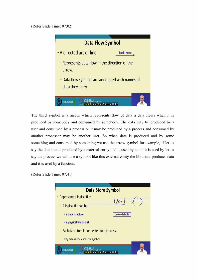
The third symbol is a arrow, which represents flow of data a data flows when it is

produced by somebody and consumed by somebody. The data may be produced by a

user and consumed by a process or it may be produced by a process and consumed by

another processor may be another user. So when data is produced and by some

something and consumed by something we use the arrow symbol for example, if let us

say the data that is produced by a external entity and is used by a and it is used by let us

say a a process we will use a symbol like this external entity the librarian, produces data

and it is used by a function.

(Refer Slide Time: 07:41)

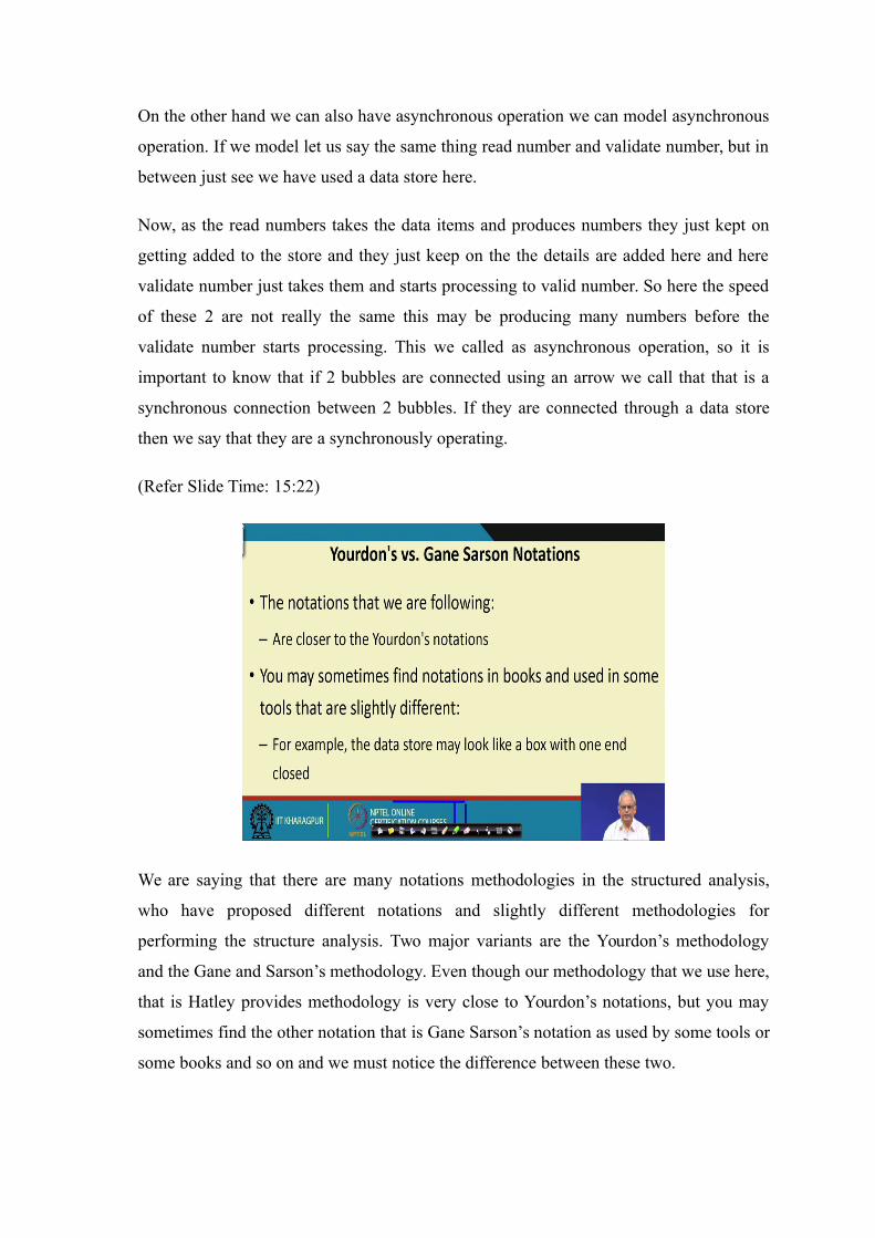
The fourth type of symbol is a data store symbol, this is just 2 parallel lines and doing

name the data store, write the name of the data store here. The data store actually

represents a data structure it can be a physical file on the disk for example, we might

have a array to contain the details of the book, array of structures to contain the book

details. So that can be represented by two parallel lines and the name of the array of book

details is the book details and the store by itself does not exist it has to be used for

something. For example, it can be used by a process, but a data store is not used by the

end user or external entity it is used by a process.

So, a books details maybe updated by a process or may be consumed by a process, so

each books each data store has to be connected to some process through a data flow

symbol.

(Refer Slide Time: 09:50)

This is 1 example users of the data store symbol, we have the books as the data store and

the process find book it takes these books and finds a book and the direction of the arrow

here shows whether the data is being read here or is being written. And one thing we

must mention here that as long as we mention a we draw arrow here, it implies all the

data is used by this all the data becomes available to the process to use it is not that just

one data from this data store and another thing we need to mention is that since all the

data traverse on this arrow we do not have to write the name of the data.

So, this data flow arrow is special which connects to a data store we do not write the

name of the data on the arrow for all other situations, where there is a arrow connecting

between 2 processors or between an end user and a process and so on we have to write

the name of the data on that data flow arrow.

(Refer Slide Time: 11:23)

And lastly the fifth symbol is the parallelogram the parallelogram represents the output

produced by the system.

(Refer Slide Time: 11:35)

For example a printout or a display and so on.

So, we just saw that the number of symbols are very small only 5 symbols, 1 is for

external entity then we have the processing symbol and then we had the data flow

symbol and then the data store symbol and finally, the output symbol.

Now before starting to model systems using the DFD notation, let us look at another 1 or

2 useful concepts. One is about synchronous operation, let us say we have this kind of

connection that there are two processes read number and validate number and they are

connected by a data flow arrow and whenever we have a data flow arrow, we write the

name of the data on that. The name of the data that flows on this arrow we write that and

we had mentioned that only when there is a data store we do not write the name of the

data otherwise we write the name of the data. And just see here that the read number

produces the number and it is consumed by the validate number here we say that these 2

processes operate lockstep or in a synchronous manner; that is until the number is

produced by read number validate number does not do anything.

Once the number is produced the validate number starts to perform its activity and it

produces the valid number. So this concept we call it synchronous operation that is the

activity of this process validate number is dependent on when the read number produces

the number.

(Refer Slide Time: 13:59)

On the other hand we can also have asynchronous operation we can model asynchronous

operation. If we model let us say the same thing read number and validate number, but in

between just see we have used a data store here.

Now, as the read numbers takes the data items and produces numbers they just kept on

getting added to the store and they just keep on the the details are added here and here

validate number just takes them and starts processing to valid number. So here the speed

of these 2 are not really the same this may be producing many numbers before the

validate number starts processing. This we called as asynchronous operation, so it is

important to know that if 2 bubbles are connected using an arrow we call that that is a

synchronous connection between 2 bubbles. If they are connected through a data store

then we say that they are a synchronously operating.

(Refer Slide Time: 15:22)

We are saying that there are many notations methodologies in the structured analysis,

who have proposed different notations and slightly different methodologies for

performing the structure analysis. Two major variants are the Yourdon’s methodology

and the Gane and Sarson’s methodology. Even though our methodology that we use here,

that is Hatley provides methodology is very close to Yourdon’s notations, but you may

sometimes find the other notation that is Gane Sarson’s notation as used by some tools or

some books and so on and we must notice the difference between these two.

(Refer Slide Time: 16:25)

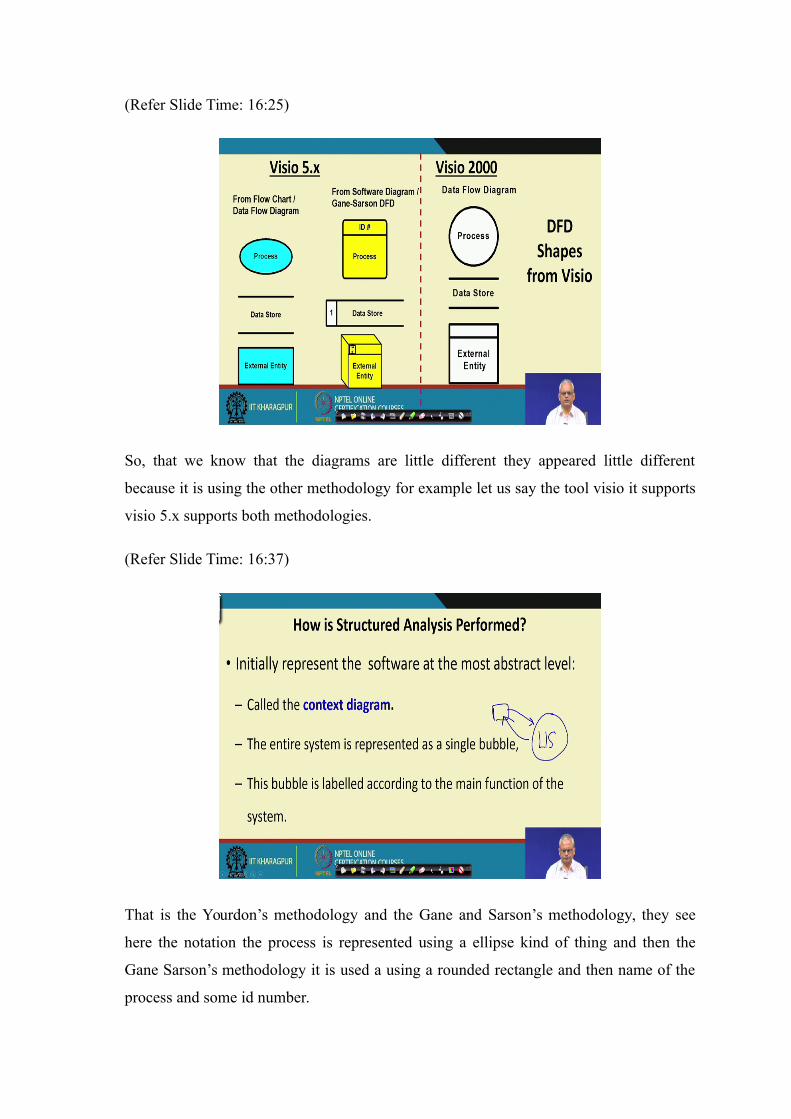
So, that we know that the diagrams are little different they appeared little different

because it is using the other methodology for example let us say the tool visio it supports

visio 5.x supports both methodologies.

(Refer Slide Time: 16:37)

That is the Yourdon’s methodology and the Gane and Sarson’s methodology, they see

here the notation the process is represented using a ellipse kind of thing and then the

Gane Sarson’s methodology it is used a using a rounded rectangle and then name of the

process and some id number.

The data store is two parallel lines in the Yourdon’s as you were discussing external

entity is a rectangle, this is the notation that were discussion on the other hand in the gain

Sarson’s just see here this is the parallel line for a data store, but the see here that it is

there are 2 vertical lines also and the the external entity is actually a rectangle, but then

the sorry it is a cube kind of thing.

So, a rectangle is; obviously, easier to draw and the cube is more cumbersome to draw. In

Visio 2000 see here it uses the Yourdon’s notations circle 2 parallel lines and then

external entity is actually slightly variant from both this. So even though the

methodologies are nearly the same and the notations are nearly the same, but then there

are small variations that we must take into consideration. The reason is that there was no

standardization effort effort. Whereas, in the object oriented design we will see that even

though there are also many variations of notations and methodologies existed, but there

was a standardization effort and therefore, the UML unified modeling language was

proposed and once that became the de facto standard everybody used UML and

therefore, the models there will appear uniform irrespective of which tool or which

project you visit.

On the other hand in procedural design there can be small variations in the appearance of

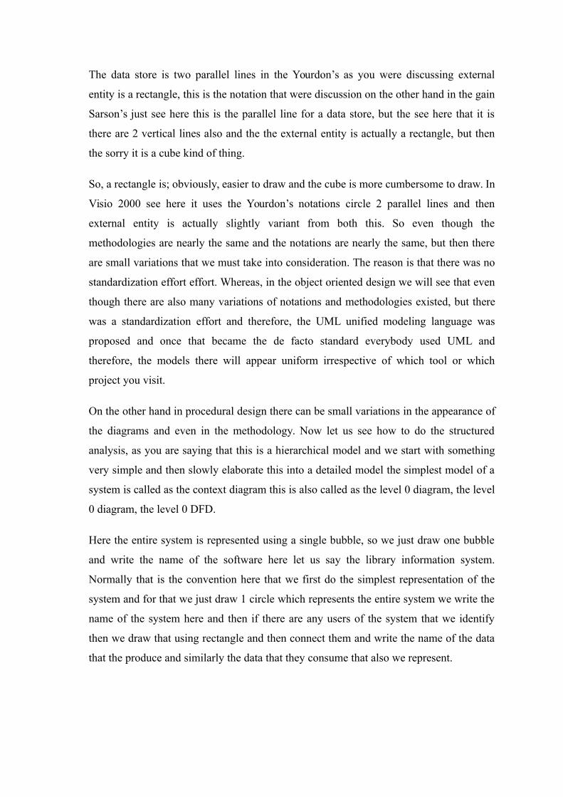
the diagrams and even in the methodology. Now let us see how to do the structured

analysis, as you are saying that this is a hierarchical model and we start with something

very simple and then slowly elaborate this into a detailed model the simplest model of a

system is called as the context diagram this is also called as the level 0 diagram, the level

0 diagram, the level 0 DFD.

Here the entire system is represented using a single bubble, so we just draw one bubble

and write the name of the software here let us say the library information system.

Normally that is the convention here that we first do the simplest representation of the

system and for that we just draw 1 circle which represents the entire system we write the

name of the system here and then if there are any users of the system that we identify

then we draw that using rectangle and then connect them and write the name of the data

that the produce and similarly the data that they consume that also we represent.

(Refer Slide Time: 21:02)

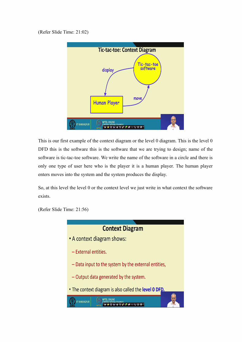
This is our first example of the context diagram or the level 0 diagram. This is the level 0

DFD this is the software this is the software that we are trying to design; name of the

software is tic-tac-toe software. We write the name of the software in a circle and there is

only one type of user here who is the player it is a human player. The human player

enters moves into the system and the system produces the display.

So, at this level the level 0 or the context level we just write in what context the software

exists.

(Refer Slide Time: 21:56)

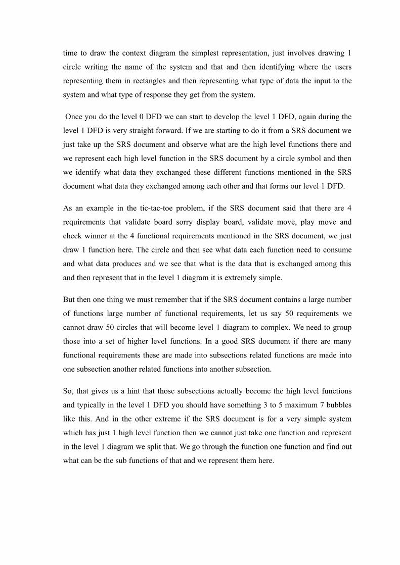
The software exists in the context of it is users and any other external entities. And then

we also mention here what type of data they input and what type of data they consume,

the human player inputs moves to the software and in response the tic-tac-toe software

produces display. So that is the context level diagram and we will do a couple of

problems and you will see that doing the context level diagram for any system is

extremely straightforward we just go through the problem description find out who are

the users and what data the input, what data they consume. And then we draw 1 circle

representing the system and write the different types of users here using rectangles and

then write the data the input and the data they produce and for this simplest the simplest

system there is only 1 type of user that is the human player.

But we will do more complex systems we there are many types of users for the software.

(Refer Slide Time: 23:20)

So, here we represent the external entities and the main system is drawn using one

process symbol, we also represent the data input by the external entities and the data

generated by the system and this will call as the level 0 DFD.

(Refer Slide Time: 23:47)

The level 0 DFD establishes the context of the system that is in the context of which

users it exists and what the you just do with the system what type of data they enter and

what type of response they get.

So, the context in which software exists is the context of the data sources and the data

sinks which are basically the users of the system.

(Refer Slide Time: 24:24)

Now, during the context level diagram at the level 0 diagram is extremely simple,

whatever be the degree of sophistication of a problem I think it should not take much

time to draw the context diagram the simplest representation, just involves drawing 1

circle writing the name of the system and that and then identifying where the users

representing them in rectangles and then representing what type of data the input to the

system and what type of response they get from the system.

Once you do the level 0 DFD we can start to develop the level 1 DFD, again during the

level 1 DFD is very straight forward. If we are starting to do it from a SRS document we

just take up the SRS document and observe what are the high level functions there and

we represent each high level function in the SRS document by a circle symbol and then

we identify what data they exchanged these different functions mentioned in the SRS

document what data they exchanged among each other and that forms our level 1 DFD.

As an example in the tic-tac-toe problem, if the SRS document said that there are 4

requirements that validate board sorry display board, validate move, play move and

check winner at the 4 functional requirements mentioned in the SRS document, we just

draw 1 function here. The circle and then see what data each function need to consume

and what data produces and we see that what is the data that is exchanged among this

and then represent that in the level 1 diagram it is extremely simple.

But then one thing we must remember that if the SRS document contains a large number

of functions large number of functional requirements, let us say 50 requirements we

cannot draw 50 circles that will become level 1 diagram to complex. We need to group

those into a set of higher level functions. In a good SRS document if there are many

functional requirements these are made into subsections related functions are made into

one subsection another related functions into another subsection.

So, that gives us a hint that those subsections actually become the high level functions

and typically in the level 1 DFD you should have something 3 to 5 maximum 7 bubbles

like this. And in the other extreme if the SRS document is for a very simple system

which has just 1 high level function then we cannot just take one function and represent

in the level 1 diagram we split that. We go through the function one function and find out

what can be the sub functions of that and we represent them here.

(Refer Slide Time: 28:21)

And once we have done the level 1 DFD where we had taken the SRS document, identify

the functions that are documented there and represent them as circles. If we want to do a

level 2 or level 3 diagram, so we look at the 1 function in the level 1 diagram and then

we identify the sub functions of that and then we identify the data input and the data

output and represent it in a different DFD diagram.

obviously, to able to identify the sub functions of a function as we go through the SRS

document we read the description of the function. And if we clearly understand that what

the function involves will be normally be able to identify the sub functions. We will do

that with the help of few examples and you will see that once you do few that, so no big

deal you can easily identify the sub functions of a function. And in that manner we keep

on building the hierarchy and we go on decomposing until we find the functions have

become very simple which take only a couple of time couple of statements to achieve

these functions at the most detailed level.

(Refer Slide Time: 30:02)

When we decompose a function, we call it as factoring or exploding a bubble each

bubble is decomposed to 3 to 7 bubbles. At this context level we have only 1 function we

have factored that into about 3 to 5 functions in the level 1 diagram and then we have

taken each of the function here at the level 1 diagram and we have factored that.

So, at any time we take in a diagram 1 of the bubble and we develop a DFD diagram for

that. So the DFD model if you can imagine it will contain many diagrams, many DFD

diagrams and each diagram will be linked by its previous level diagram.

So the level 1 diagram is a elaboration of the level 0 diagram similarly the set of the level

2 diagrams are an elaboration of the level 1 diagram and so on.

(Refer Slide Time: 31:21)

We must take care well decomposition, that if there is a we take 1 bubble in a level we

should not decompose it into another just 1 bubble in the next level it should be between

3 to 5, it should not be just 1 or 2 otherwise the decomposition loses it is purpose.

Ah So far in this lecture we looked at the DFD symbols so that there are 5 very simple

symbols and we just identify simple rules by which they are connected. The dataflow

arrows when they connect a process to another process is called a synchronous flow must

write the name of the data and the arrow it is connected via a data store then it represents

an asynchronous operation. And we discussed also how to develop the context diagram

and the level 1 diagram and we also discussed about how to do the decomposition for

any level DFD, we just take 1 bubble at a time and then we decompose it anything

between 3 to 5 sub functions and represent them for the next level d DFD and so on.

We will stop here and continue from this point we will see how to give an example how

do we develop its DFD model

Thank you