1 Software for genome-wide association studies in autopolyploids and its application to potato Umesh R. Rosyara, Walter S. De Jong, David S. Douches, Jeffrey B. Endelman * U.R. Rosyara, J.B. Endelman, Dept. Horticulture, Univ. Wisconsin, Madison, WI 53706 W.S. De Jong, School of Integrative Plant Science, Cornell Univ., Ithaca, NY 14853 D.S. Douches, Dept. Plant, Soil and Microbial Sciences, Michigan State Univ., East Lansing, MI 48824 Received August 21, 2015 Accepted November 24, 2015 (Plant Genome) *Corresponding author ([email protected]) Abbreviations: DAPC, discriminant analysis of principal components; FW, fresh weight; GWAS, genome-wide association studies; LDA, linear discriminant analysis; P3D, population parameters previously determined; REML, restricted maximum likelihood; SolCAP, Solanaceae Coordinated Agricultural Project; QTL, quantitative trait locus (or loci); SNP, single nucleotide polymorphism.
Transcript
1"
Software for genome-wide association studies in autopolyploids and its
application to potato
Umesh R. Rosyara, Walter S. De Jong, David S. Douches, Jeffrey B. Endelman*
Three tetraploid kinship (or relationship) models were compared. The first is the canonical
relationship matrix used in genome-wide prediction studies (VanRaden, 2008), which we call the
realized relationship model:
K =MMT (Realized Relationship)
8"
In the above equation, M is the n x m genotype matrix for a population of size n with m markers,
where the genotypes (Mij) have been “centered” by subtracting the population mean for each
marker (Endelman and Jannink, 2012). The second approach is based on the concept of a
molecular similarity index (Oliehoek et al., 2006). If a,b,c,d denote the four homologs at locus z
in one individual, and e,f,g,h denote the homologs in a second individual, the similarity between
the two individuals at that locus is
Kz =116
Ixyy∈{e, f ,g,h}∑
x∈{a,b,c,d}∑ (Molecular Similarity)
where the indicator function Ixy equals one when the two subscripts are equal and is zero
otherwise. The average similarity across m loci is K =m−1 Kzz∑ . Whereas the first two models
may be considered additive models of relationship, the third model—the Gaussian kernel—
involves multigenic interactions (Gianola and van Kaam, 2008; Piepho, 2009). Its formula is
Kij = exp − Dij /θ( )2"
#$%&' (Gaussian Kernel)
where Dij is the Euclidean distance, normalized to the interval [0,1]:
Dij2 = 16m( )−1 Mik −M jk( )
2
k∑ . The value for the scale parameter θ, which determines how
quickly kinship decays with genetic distance, was determined by REML as described in
Endelman (2011).
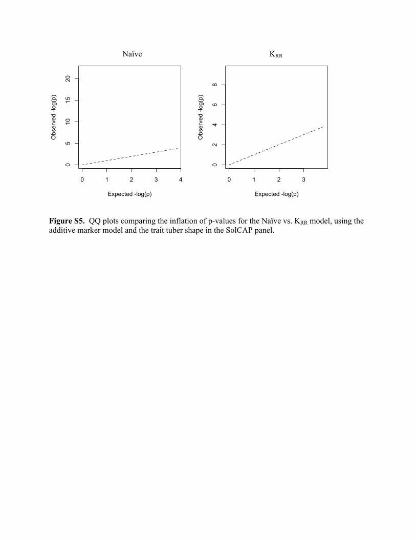
A key diagnostic for GWAS is a quantile-quantile (QQ) plot of the observed vs. expected
–log p values, which should follow a uniform distribution under the null hypothesis. The
“inflation” of high p-values above the y=x line in such a plot is an indicator of the failure of the
model to control for population structure. Inflation was quantified by the linear regression
9"
coefficient of the observed vs. expected –log10 p-values, denoted λ, which has a value of 1 under
the null hypothesis (Riedelsheimer et al., 2012).
The average inflation across different GWAS models and traits was compared by analysis
of variance, according to
λij = µ + ti +β j +εij
where ti is the effect for trait i and βj is the effect for model j. The naïve GWAS model was not
included in the analysis as it produced residuals with much larger variance (thereby violating an
assumption of ANOVA). R package lsmeans was used to make means comparisons, with p-
values adjusted for multiple testing by Tukey’s method.
Three different methods are available in GWASpoly for establishing a p-value detection
threshold for statistical significance. The first is the Bonferroni correction, which uses a
threshold of α/m to ensure the genome-wide type I error with m markers is no greater than α.
The second approach is the random permutation test, in which phenotypes are randomly
permuted to explicitly construct the genome-wide null distribution of p-values (Churchill and
Doerge, 1994). The third option uses the q-value package (Storey and Tibshirani, 2003) to
control the genome-wide false discovery rate (rather than type I error = probability of false
positive). For the simulations, due to their computationally intensive nature, we used the
Bonferroni correction with α = 0.05. For the analysis of the real potato data, we used the
permutation test with 1000 permutations and genome-wide α = 0.05.
Simulated populations
Simulated populations and phenotypes were used to validate the software. Random
mating autotetraploid populations were simulated using the software PedigreeSim (Voorrips and
10"
Maliepaard, 2012), according to the scheme illustrated in Supplemental Figure S1. The base
population consisted of five individuals, from which 10 mating pairs were randomly selected,
and 10 progeny per pair were randomly generated to create a population of 100 individuals in
Generation 1. In generations 2 through 999, 100 mating pairs were randomly selected, each
contributing 1 offspring, to keep the population size constant at 100. For the last (1000th)
generation, N mating pairs were randomly selected, each contributing one offspring to create a
population of size N. Results are shown for N = 200, 400, and 600. The simulated genome
contained three chromosomes, each 100 cM in length, with 100 loci per cM. Recombination was
simulated according to Haldane’s mapping function, using the default meiosis parameters
governing the formation of quadrivalents. Marker density was varied by subsampling loci (m =
3, 10, 50 per cM).
To estimate power in each simulated population, one marker was randomly designated as
the causal QTL and the remaining markers were converted to bi-allelic SNPs by randomly
assigning the 20 founder alleles to bi-allelic states (A/B), thereby creating markers with an
average minor allele frequency of 0.5. Two different schemes were used to simulate genotypic
values. In the first, the causal QTL was also converted to a bi-allelic locus as above, and allelic
effects were sampled from the standard normal distribution. This scheme was used to generate
Tables 1 and 2. In the second scheme, which was used for Figure 2, each of the 20 founder
alleles was assigned a different effect, drawn from the standard normal distribution. The
phenotypic value for each genotype was the sum of its genotypic value and a random deviate,
with variance chosen such that the ratio between the genetic and phenotypic variances of the
population was h2 = 0.3. Because there were no sub-populations in the simulated population, we
used a K-only GWAS model with the realized relationship matrix. A QTL was considered
11"
detected if a SNP within 5 cM of the unobserved QTL had –log p-value above the significance
threshold. Conversely, significant markers greater than 5 cM from the QTL were considered
false positives. We report the average power and false positive rate based on 1000 replications,
with standard errors computed from the binomial distribution.
Potato diversity panel
The genotypic and phenotypic data were collected as part of the Solanaceae Coordinated
Agricultural Project (SolCAP). The SolCAP potato diversity panel consists of both diploid and
tetraploid wild species, genetic stocks, and cultivated potato lines with release dates ranging
from 1857 to 2011 (Hirsch et al., 2013). The panel was genotyped with an Infinium SNP array
of 8303 markers (Hamilton et al., 2011; Felcher et al., 2012), and tetraploid marker dosage was
determined by Hirsch et al. (2013), principally by visual inspection of the cluster boundaries.
Our analysis of population structure was conducted using all 221 tetraploid lines in the panel
(Supplemental Table S1), while GWAS results are based on the 187 tetraploid lines with both
marker and phenotypic data.
Broad-sense heritability and GWAS results are presented for thirteen quantitative traits,
which were measured in up to four environments (New York-2010, Wisconsin-2010, New York-
2011, Wisconsin-2011). A randomized complete block design with two replicates was used in
each environment, although not all traits were measured in every environment (the number of
environments per trait is shown in Table 4). In addition to the four traits analyzed by Hirsch et
al. (2013), which were chip color (1–5 scale), tuber shape (1–5 scale), tuber sucrose and glucose
(mg g-1 FW), we present GWAS results for total yield (kg), tuber size and eye depth (1–9 visual
scale), vine maturity 95 and 120 days after planting (1–9 visual scale), tuber length (mm), tuber
12"
width (mm), tuber fructose and malic acid content (mg g-1 FW). Phenotypic data were analyzed
with the following linear model:
yijk = µ +Gi +Ej + b(E) jk +GEij +εijk
where yijk is the observation for genotype i in block k of environment j. Variance components
were estimated by REML using R package lme4 (R Development Core Team, 2014). The
residuals appeared to be normally distributed for all traits except fructose and glucose, for which
a log transformation was used to satisfy model assumptions. Because the experimental design
was unbalanced for several traits, the reliability, or heritability, of each genotype was estimated
from the prediction error variance (PEV) of the BLUP solution for Gi (Clark et al., 2012): h2 = 1
– PEV/VG. For each trait we report the average heritability for the population. To generate
phenotypic values for GWAS, Gi was modeled as a fixed effect (all other effects were random),
and the best linear unbiased estimator (BLUE) was computed with lme4 (Supplemental Table
S2).
Three different population structure matrices (Q) were compared. The first corresponds to
the four sub-populations identified with the program STRUCTURE (Pritchard et al., 2000), as
reported by Hirsch et al. (2013). The second matrix was constructed from a principal component
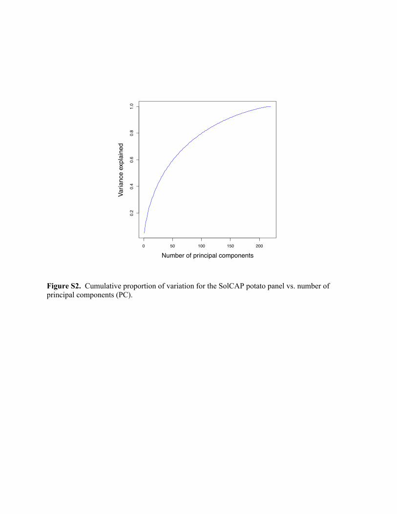
analysis (PCA), using centered and scaled marker scores (Price et al., 2006). Since a scree plot
of the cumulative percent variation vs. model complexity (Supplemental Figure S2) showed a
gradual increase and no obvious choice for a low-dimensional model, we used four principal
components to be consistent with the four covariates used with the other Q models. The third
matrix was based on the Discriminant Analysis of Principal Components (DAPC) method in R
package adegenet (Jombart et al., 2010). Since DAPC is less widely used than PCA or
STRUCTURE, we describe it in more detail. In the first step, k-means clustering was used to
13"
identify groups. The value k = 4 minimized the Bayesian Information Criterion (BIC) and was
thus used for GWAS (group membership probabilities in Supplemental Table S2). However, for
the purpose of discussing population structure we selected k = 6, which was still within the
shallow minimum of the BIC curve (Supplemental Figure S3). In the second step of the DAPC
method, linear discriminants were computed based on a reduced-rank representation of the
marker matrix (Jombart et al., 2010). Unlike PCA, which maximizes the total variation in the
dataset, linear discriminants maximize the ratio of the between-group to within-group sum-of-
squares. A cross-validation study revealed that the classification error by LDA was minimized
over a range of model complexities (Supplemental Figure S4); we selected 60 PCs for LDA at
the upper end of the range.
For each trait, four GWA analyses were conducted, based on the additive, simplex
dominant, duplex dominant, and the general SNP models. When multiple significant markers
were detected within a 10 Mb region, only the most significant (i.e., lowest p-value) was
reported, along with the corresponding SNP model.
Statistical power was estimated for the SolCAP panel genotypes using a similar method as
for the simulated populations. An additive QTL with h2 = 0.3 was simulated at each marker,
which was considered detected if any marker up to 2.5 Mb from the QTL exceeded the detection
threshold of α = 0.05/3242 (i.e., the Bonferroni correction for a genome-wide scan). Extending
the detection interval up to 5 Mb from the QTL did not change the median power for the genome
(Supplemental Table S3). The average power for each QTL was based on 1000 simulations.
14"
Results and Discussion
Validation with simulated data
The GWAS software was validated using simulated phenotypes and genotypes from a
random mating autotetraploid population (details in Methods). Our first objective was to
determine the quality of the P3D approximation for the mixed model (Zhang et al., 2010; Kang
et al., 2010), which is widely used in diploid GWAS to reduce the computing time. The P3D
approximation involves estimating the variance components only once by REML, and then using
those values for each single-marker hypothesis test. Table 1 compares the statistical power and
false positive rate of the full mixed model vs. the P3D model for three different types of
simulated QTL: additive, simplex dominant, and duplex dominant (see Methods for more
information on these models). Using the same p-value detection threshold for both methods, we
observed slightly lower statistical power (0.01–0.05) when using the P3D model but also fewer
false positives. If the –log10p threshold for the P3D model were lowered to achieve the same
false positive rate for the two methods, the difference in statistical power would be even smaller.
For this relatively small dataset of 400 individuals and 1800 markers (600 for each of three
linkage groups), the P3D approximation reduced the computing time by a factor of 20. Thus,
given its favorable performance, the P3D approach was used for the remainder of the study.
One of the unique features of the software is its ability to conduct the single marker test for
association using different models of gene action. Our hypothesis was that the probability of
detecting QTL would be higher if the marker model matched the gene action at unobserved QTL.
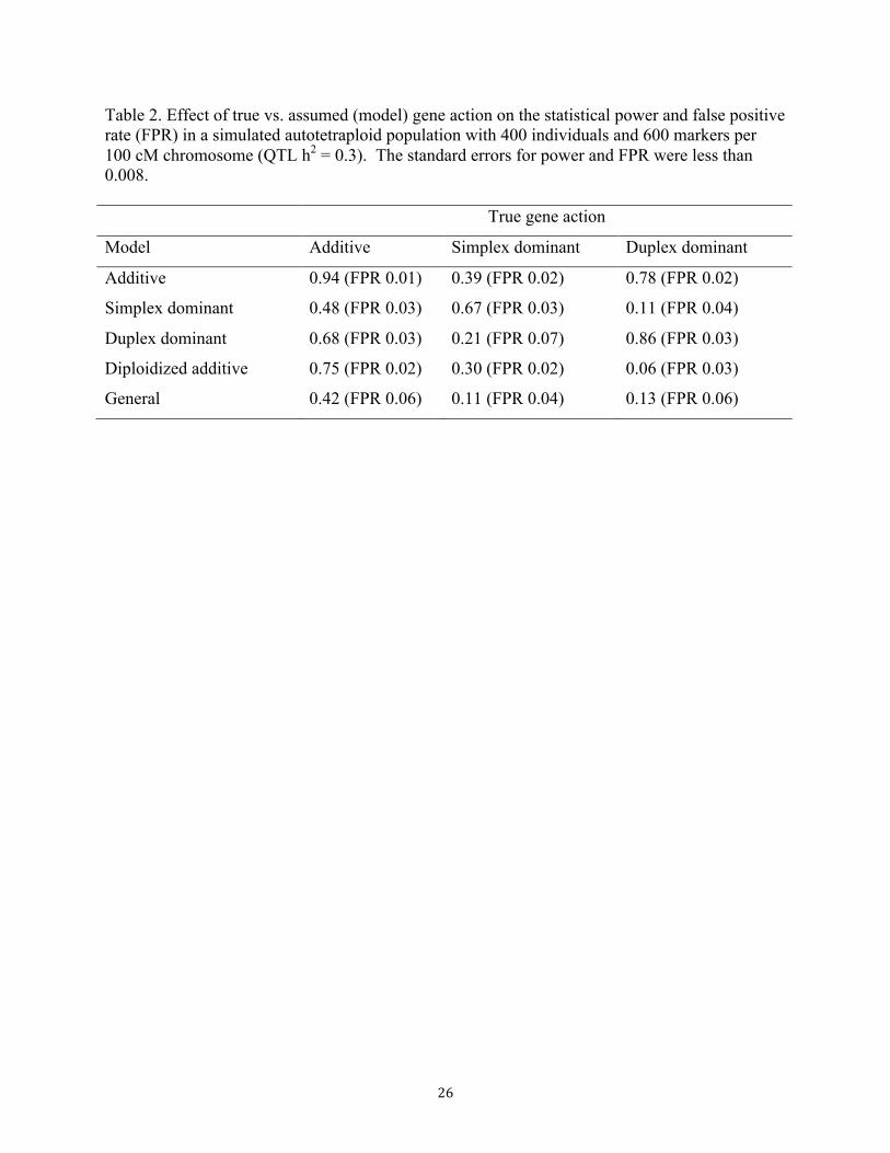
The results shown in Table 2 confirm this hypothesis: for an additive QTL, analysis with an
additive model resulted in a statistical power of 0.94, while the next most powerful model
detected the QTL with probability 0.75 (standard errors < 0.01). For a simplex dominant QTL,
15"
use of the simplex model in the analysis increased power by 0.28 over the next best model
(additive). Table 2 also illustrates the consequences of neglecting dosage information for the
heterozygous genotypes, i.e., “diploidizing” the data. If the underlying QTL is simplex
dominant, there is no loss of power with diploidized marker data as the simplex dominant model
implies all heterozygous genotypes are equivalent. However, when the QTL was additive or
duplex dominant, the best diploid model had significantly less power than the best tetraploid one
(losses of 0.19 and 0.67, respectively). Table 2 also shows the potential disadvantage of relying
solely on the general tetraploid model, which makes no assumptions about gene action and thus
encompasses the other models. This flexibility comes with a penalty of substantially lower
statistical power (more than 0.5 less than the best model) because four degrees of freedom (dof)
are needed for the single marker test. This conclusion still holds when the general model is
compared against a combination of multiple single-dof models with a higher detection threshold
to maintain the same false positive rate (data not shown).
Our third objective was to investigate the effects of marker density and population size on
statistical power in autotetraploid GWAS. In diploids it is well established that both factors
contribute to higher power (Klein, 2007; Spencer et al., 2009), and this trend was also observed
in simulated autotetraploid populations (Figure 2). The left-most bars in panels A and B of
Fig. 2 correspond to a common scenario of 300 markers per 100 cM chromosome and 200
individuals, which is approximately the size of the real potato dataset analyzed below. Figure
2A shows the effect of increasing population size, while Fig. 2B illustrates higher maker density.
For the same proportional increase (e.g., twofold), population size had a bigger effect on power
than marker density. The two different series in Fig. 2 (solid vs. open) correspond to different
types of QTL models. In both cases the markers are bi-allelic, but the solid bars correspond to
16"
bi-allelic QTL while the open bars are multi-allelic QTL. The loss in power for the latter
scenario can be viewed as analogous to the loss in power for the off-diagonal elements in
Table 2: in both cases there is a mismatch between the markers in the GWAS model and gene
action at the unobserved QTL. This mismatch can potentially be overcome through the use of
multi-marker haplotypes in GWAS (Lorenz et al., 2010).
GWAS of a tetraploid potato diversity panel
The SolCAP potato diversity panel included 221 tetraploid lines and 3441 tetraploid SNP
markers with minor allele frequency greater than 0.05. Based on version 4.03 of the potato
reference genome (Potato Genome Sequencing Consortium, 2011; Sharma et al., 2013), the
median distance between markers was 67 kb, with a minimum of 3 bp and maximum of 8.2 Mb.
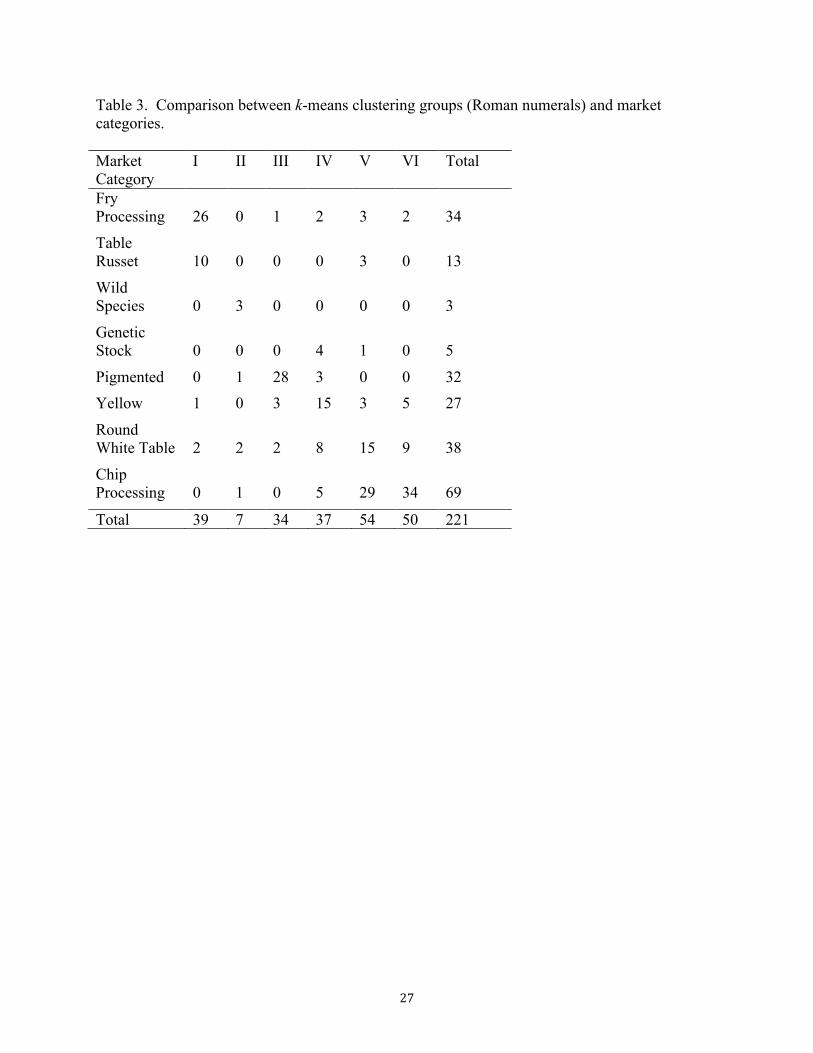
The diversity panel was comprised of potatoes from eight different market categories, listed
in Table 3. Previously, the program STRUCTURE had been used to identify subpopulations in
this dataset (Hirsch et al., 2013). A commonly used alternative to STRUCTURE for GWAS is
principal component analysis, or PCA. Figure 3A shows the projection of the population onto
the first two principal components, which only account for 8% of the total variation in the
marker data (scree plot in Supplemental Figure S2).
To achieve better separation between sub-populations, we used a technique called
discriminant analysis of principal components, or DAPC (Jombart et al. 2010). In the first step,
clusters based on the marker data were compared against the market categories. Table 3 and
Figure 3B show the results for k = 6 clusters. As expected, the DAPC technique produced
greater separation among groups than PCA, with Groups I–III clearly separated and Groups IV-
VI apparently more closely related. Group I primarily contains the fry processing and table
17"
russets, which are closely related and continue to be intermated by breeders. Group II was a
small group containing the majority of the wild species in the panel, and Group III contained
most of the pigmented (red and purple) types. Group IV contained the majority of the yellow
potatoes, along with some round white potatoes for both tablestock and chip processing. Groups
V and VI were predominantly round white potatoes, used for both tablestock and chip
processing. Hirsch et al. (2013) also observed minor divergence within the round white types
based on hierarchical clustering.
One of the hallmarks of using ordinary linear regression (aka, the naïve model) as a test of
association in structured populations is the inflation of the –log(p) values relative to the expected
value under the null hypothesis (Supplemental Figure S5; Freedman et al., 2004; Clayton et al.,
2005). The use of sub-population group membership as a covariate in the analysis helps to
reduce this inflation. Each boxplot in Figure 4 shows the distribution of inflation factors across
the 13 traits analyzed in this study. All three of the Q-models tested—DAPC, PCA, and
STRUCTURE—were able to reduce inflation relative to the naïve model, with DAPC and PCA
slightly better than STRUCTURE. The DAPC approach (QDAPC) was selected for subsequent
analyses.
As first shown by Yu et al. (2006), a random polygenic effect with covariance proportional
to a kinship matrix K can also reduce inflation. The results in Figure 4 show that all three
kinship matrices we tested were effective, with perhaps a slight advantage to the realized
relationship model (KRR = MMT for genotype matrix M), which had significantly less inflation
than any of the Q models. Subsequent analyses were conducted using the QDAPC + KRR model.
Several categories of traits were measured on the diversity panel, including agronomic (e.g.,
total yield, vine maturity), morphological (e.g., tuber shape and eye depth), and biochemical
18"
(e.g., tuber sucrose and glucose) properties. Table 4 presents the broad-sense heritability on an
entry-mean basis for each trait, which ranged from 0.60 for tuber malic acid content to 0.94 for
tuber shape.
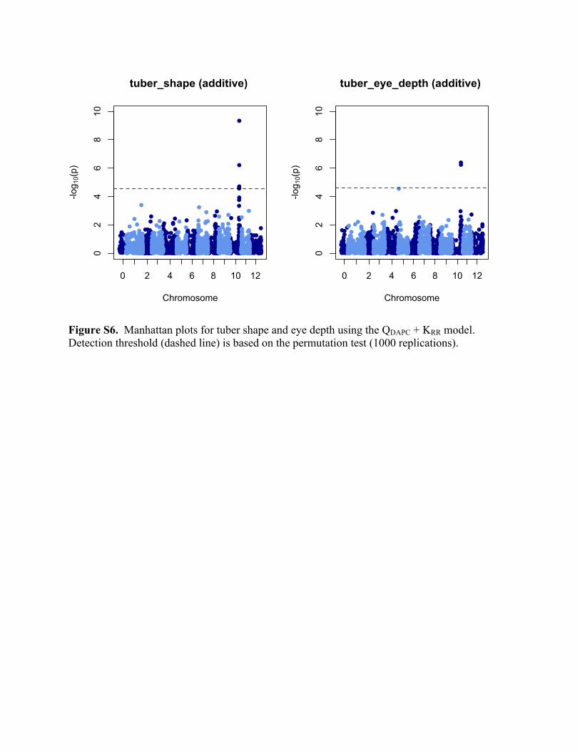
Significant QTL were detected for 7 of the 13 traits, although many of the QTL were only
marginally significant (Table 4; results for all markers in Supplemental Table S4). Significant
QTL were not detected for the three tuber sugar traits (sucrose, glucose, and fructose) even
though they had heritability comparable to the other traits. This was unexpected as metabolic
traits typically have fewer causal loci with larger (and thus more easily detectable) effects
compared to a complex trait such as yield (Riedelsheimer et al., 2012). The most significant
QTL were for tuber shape and tuber eye depth, both at 48.9 Mb on chromosome 10
(Supplemental Figure S6). Several biparental linkage mapping studies have mapped major QTL
for these traits to the same region (Van Eck et al., 1994; Śliwka et al., 2008; Li et al., 2005;
Prashar et al., 2014), although the molecular identities of the QTL have not yet been published.
QTL studies in potato frequently detect a major locus affecting plant maturity on chromosome 5
(Bradshaw et al., 2008), which was identified as the StCDF1 gene by Kloosterman et al. (2013).
This locus was not detected in our analysis of the SolCAP plant maturity data, although minor
QTL were identified on chromosomes 7, 9 and 11.
To better understand the scarcity of major QTL in the GWAS results for the SolCAP panel,
a power simulation was performed using simulated QTL and phenotypes but with the actual
marker data. For a monogenic trait with h2 = 0.3, the genome-wide median for the probability of
QTL detection was only 0.01 (results for all loci in Supplemental Table S3). Although low
power was expected considering the small size of the population (N = 187), this result was even
lower than anticipated. To determine if marker density also played a role, the power was plotted
19"
against the distance between the QTL and its closest marker (Fig. 5). The red trendline in Fig. 5,
which is the 95th percentile, shows that power was lower in regions of lower marker density.
We conclude that, in addition to increasing the population size, higher marker density could also
improve future GWAS studies in potato.
The GWASpoly software is being distributed under the GNU Public License and can be
downloaded from http://potatobreeding.cals.wisc.edu/software.
Author contributions. Designed the research: JBE. Contributed phenotypic data: WSD, DSD.
Developed the software and analyzed the data: URR, JBE. Wrote the manuscript: URR, JBE.
Acknowledgments
Financial support was provided to U.R.R. by USDA-NIFA-SCRI Grant No. 2011-51181-30629
(Improved Breeding and Variety Evaluation Methods to Reduce Acrylamide Content and
Increase Quality in Processed Potato Products) and to J.B.E. by USDA-NIFA-Hatch Accession
No. 1002731 (Genome-wide Association Analysis and Breeding in Potato). Collection of the
phenotype and marker data was supported by USDA-NIFA-AFRI Grant No. 2009-85606-05673
(Translating Solanaceae Sequence Diversity and Trait Variation into Applied Outcomes through
Integrative Research, Education, and Extension). We thank Paul Bethke and Shelley Jansky for
contributing phenotypic data.
20"
References
Allison, D. B. 1997. Transmission-disequilibrium tests for quantitative traits. Am. J. Hum. Genet. 60 676–690.
Balding, D. J. 2006. A tutorial on statistical methods for population association studies. Nat. Rev. Genet. 7:781–791.
Bradbury, P.J., Z. Zhang, D.E. Kroon, T.M. Casstevens, Y. Ramdoss, and E.S. Buckler. 2007. TASSEL: Software for association mapping of complex traits in diverse samples. Bioinform. 23:2633-2635.
Bradshaw, J.E., C.A. Hackett, B. Pande, R. Waugh, and G.J. Bryan. 2008. QTL mapping of yield, agronomic and quality traits in tetraploid potato (Solanum tuberosum subsp. tuberosum) Theor. Appl. Genet. 116:193–211.
Churchill, G.A., and R.W. Doerge. 1994. Empirical threshold values for quantitative trait mapping. Genetics 138: 963–971.
Clark, S.A., J.M. Hickey, H.D. Daetwyler, and J.H.J. van der Werf. 2012. The importance of information on relatives for the prediction of genomic breeding values and the implications for the makeup of reference data sets in livestock breeding schemes. Genet. Sel. Evol., 44:4. doi: 10.1186/1297-9686-44-4."
Clayton D.G., N.M. Walker, D.J. Smyth, R. Pask, J.D. Cooper, L.M. Maier, L.J. Smink, A.C. Lam, N.R. Ovington, H.E. Stevens, S. Nutland,, J.M. Howson, M. Faham, M. Moorhead, H.B. Jones, M. Falkowski, P. Hardenbol, T.D. Willis, and J.A. Todd. 2005. Population structure, differential bias and genomic control in a large-scale, case–control association study. Nat. Genet. 37:1243-1246.
Endelman, J.B. 2011. Ridge regression and other kernels for genomic selection with R package rrBLUP. Plant Genome 4: 250–255.
Endelman, J.B., and J.-L. Jannink. 2012. Shrinkage estimation of the realized relationship matrix. G3 (Bethesda) 2:1405–1413.
Felcher K. J., J. J. Coombs, A. N. Massa, C. N. Hansey, J. P. Hamilton, R.E. Veilleux, C.R. Buell, and D. S. Douches. 2012. Integration of two diploid potato linkage maps with the potato genome sequence. PLoS ONE 7:e36347.
Freedman, M.L., D. Reich, K.L. Penney, G.J. McDonald, A.A. Mignault, N. Patterson, S.B. Gabriel, E.J. Topol, J.W. Smoller, C.N. Pato, M.T. Pato, T.L. Petryshen, L.N. Kolonel, E.S. Lander, P. Sklar, B. Henderson, J.N. Hirschhorn, and D. Altshuler. 2004. Assessing the impact of population stratification on genetic association studies. Nat. Genet. 36:388-393.
Gallais, A. 2003. Quantitative genetics and breeding methods in autopolyploid plants. INRA, Paris, France.
Gianola, D., and J.B.C.H.M. van Kaam. 2008. Reproducing Kernel Hilbert Spaces Regression methods for genomic assisted prediction of quantitative traits. Genetics 178:2289–2303.
Hamilton, J. P., C. N. Hansey, B. R. Whitty, K. Stoffel, A. N. Massa, A. Van Deynze, W. S. De Jong, D. S. Douches, and C. R. Buell. 2011. Single nucleotide polymorphism discovery in
21"
elite North American potato germplasm. BMC Genomics 12: 302. doi:10.1186/1471-2164-12-302.
Hirsch, C.N., C.D. Hirsch, K. Felcher, J. Coombs, D.Zarka, , A.Van Deynze, W. De Jong, R.E.Veilleux, S. Jansky, P. Bethke, D.S. Douches, and C.R. Buell. 2013. Retrospective view of North American potato (Solanum tuberosum L.) breeding in the 20th and 21st centuries. G3 (Bethesda) 3:1003-1013.
Jombart, T., S. Devillard, and F. Balloux. 2010. Discriminant analysis of principal components: a new method for the analysis of genetically structured populations. BMC Genet. 11:94. doi:10.1186/1471-2156-11-94.
Kang, H.M., J.H. Sul, S.K. Service, N.A. Zaitlen, S. Kong, N.B. Freimer, C. Sabatti, and E. Eskin. 2010. Variance component model to account for sample structure in genome-wide association studies. Nat. Genet. 42:348-354.
Kang, H.M., N.A. Zaitlen, C.M. Wade, A. Kirby, D. Heckerman, M.J. Daly, and E. Eskin. 2008. Efficient control of population structure in model organism association mapping. Genetics 178:1709–1723.
Klein, R.J. 2007. Power analysis for genome-wide association studies. BMC Genet. 8:58. doi:10.1186/1471-2156-8-58
Kloosterman, B., J.A. Abelenda, M.D.M.C. Gomez, M. Oortwijn, J.M. de Boer, K. Kowitwanich, B. Horvath, H.J. van Eck, C. Smaczniak, S. Prat, R.G.F. Visser, and C.W.B. Bachem. 2013. Naturally occurring allele diversity allows potato cultivation in northern latitudes. Nature 495:246–250.
Li, M., X. Liu, P. Bradbury, J. Yu, Y.-M. Zhang, R.J. Todhunter, E.S. Buckler, and Z. Zhang. 2014. Enrichment of statistical power for genome-wide association studies. BMC Biol. 12:73. doi:10.1186/s12915-014-0073-5
Li, X.Q., H. De Jong, D.M. De Jong, and W.S. De Jong. 2005. Inheritance and genetic mapping of tuber eye depth in cultivated diploid potatoes. Theor. Appl. Genet. 110:1068–1073.
Li, X., Y. Wei, K.J. Moore, R. Michaud, D.R. Viands, J.L. Hansen, A. Acharya, and E.C. Brummer. 2011. Association mapping of biomass yield and stem composition in a tetraploid alfalfa breeding population. Plant Genome 4: 24–35.
Lipka, A. E., F. Tian, Q. Wang, J. Peiffer, M. Li, P.J. Bradbury , M.A. Gore , E.S. Buckler , and Z. Zhang. 2012. GAPIT: genome association and prediction integrated tool. Bioinform. 28: 2397–2399.
Lorenz, A.J., M.T. Hamblin, and J-L. Jannink. 2010. Performance of single nucleotide polymorphisms versus haplotypes for genome-wide association analysis in barley. PLoS ONE 5(11): e14079.
Malosetti, M., C. G. van der Linden, B. Vosman, and F. van Eeuwijk. 2007. A mixed-model approach to association mapping using pedigree information with an illustration of resistance to Phytophthora infestans in potato. Genetics 175: 879–889.
McCulloch, C.E., and S.R. Searle. 2001. Generalized, Linear, and Mixed Models. John Wiley and Sons, New York, NY.
22"
Myles, S., J. Peiffer, P. J. Brown, E.S. Ersoz, Z. Zhang, D. E. Costich, and E.S. Buckler. 2009. Association mapping: critical considerations shift from genotyping to experimental design. Plant Cell 21: 2194–2202.
Oliehoek, P.A., J.J. Windig, J.A. van Arendonk, and P. Bijma. 2006. Estimating relatedness between individuals in general populations with a focus on their use in conservation programs. Genetics 173:483–496.
Pajerowska-Mukhtar, K., B. Stich, U. Achenbach, A. Ballvora, J. Lubeck, J. Strahwald, E. Tacke, H.R. Hofferbert, E. Ilarionova, D. Bellin, B. Walkemeier, R. Basekow, B. Kersten, and C. Gebhardt. 2009. Single nucleotide polymorphisms in the allene oxide synthase 2 gene are associated with field resistance to late blight in populations of tetraploid potato cultivars. Genetics 181:1115–1127.
Piepho, H.P. 2009. Ridge regression and extensions for genomewide selection in maize. Crop Sci. 49:1165–1176.
Potato Genome Sequencing Consortium. 2011. Genome sequence and analysis of the tuber crop potato. Nature 475:189–195.
Prashar, A., C. Hornyik, V. Young, K. McLean, S. K. Sharma, M. F B. Dale, and G. J. Bryan. 2014. Construction of a dense SNP map of a highly heterozygous diploid potato population and QTL analysis of tuber shape and eye depth. Theor. Appl. Genet. 127:2159-2171.
Price, A.L., N.J. Patterson, R. M. Plenge, M.E. Weinblatt, N.A. Shadick, and D. Reich. 2006. Principal components analysis corrects for stratification in genome-wide association studies, Nature Genet. 38:904–909.
Pritchard, J.K., P. Stephens, and P. Donnelly. 2000. Inference of population structure using multilocus genotype data. Genetics 155:945–959.
R Development Core Team. 2014. R: A language and environment for statistical computing. R Foundation for Statistical Computing, Vienna, Austria.
Riedelsheimer, C., J. Lisec, A. Czedik-Eysenberg, R.Sulpice, A. Flis, C. Grieder, T. Altmann, M. Stitt, L. Willmitzer, and A.E. Melchinger. 2012. Genome-wide association mapping of leaf metabolic profiles for dissecting complex traits in maize. Proc. Natl. Acad. Sci. USA 109:8872-8877.
Sharma, S.K., D. Bolser, J . de Boer, M. Sønderkaer, W . Amoros, M.F. Carboni, J.M. D'Ambrosio, G. de la Cruz, A. Di Genova, D.S. Douches, M. Eguiluz, X. Guo, F . Guzman, C.A. Hackett, J.P. Hamilton, G. Li, Y. Li, R. Lozano, A. Maass, D. Marshall, D. Martinez, K. McLean, N. Mejía, L. Milne, S. Munive, I. Nagy, O. Ponce, M. Ramirez, R. Simon, S.J. Thomson, Y. Torres, R. Waugh, Z. Zhang, S. Huang, R.G.F. Visser, C.W.B, Bachem, B. Sagredo, S.E. Feingold, G. Orjeda, R.E .Veilleux, M. Bonierbale, J.M.E. Jacobs, D. Milbourne, D.M.A Martin, and G.J. Bryan. 2013. Construction of reference chromosome-scale pseudomolecules for potato: Integrating the potato genome with genetic and physical maps. G3 (Bethesda) 3:2031–2047.
Simko, I., K. G. Haynes, and R. W. Jones. 2006 Assessment of linkage disequilibrium in potato genome with single nucleotide polymorphism markers. Genetics 173:2237–2245.
23"
Śliwka, J., I. Wasilewicz!Flis, H. Jakuczun, C. Gebhardt. 2008. Tagging quantitative trait loci for dormancy, tuber shape, regularity of tuber shape, eye depth and flesh colour in diploid potato originated from six Solanum species. Plant Breed. 127:49-55.
Spencer, C.C., Z. Su, P. Donnelly, and J. Marchini. 2009. Designing genome-wide association studies: sample size, power, imputation, and the choice of genotyping chip. PLoS Genet. 5(5): e1000477.
Spielman, R. S., R. E. McGinnis, and W. J. Ewens. 1993. Transmission test for linkage disequilibrium: the insulin gene region and insulin-dependent diabetes mellitus (IDDM). Am. J. Hum. Genet. 52:506–516.
Stich, B., and C. Gebhardt. 2011. Detection of epistatic interactions in association mapping populations: an example from tetraploid potato. Heredity 107: 537–547.
Stich, B., J. Mohring, H.-P. Piepho, M. Heckenberger, E. S. Buckler, and A.E. Melchinger. 2008. Comparison of mixed-model approaches for association mapping. Genetics 178:1745–1754.
Storey, J.D., and R. Tibshirani. 2003. Statistical significance for genomewide studies. Proc. Natl. Acad. Sci. USA 100: 9440–9445.
Uitdewilligen, J.G.A.M.L., A.-M. A. Wolters, , B.B. D’hoop, T. J. A. Borm, , R. G. F. Visser, and H. J. van Eck. 2013. A next-generation sequencing method for genotyping-by-sequencing of highly heterozygous autotetraploid potato. PLoS ONE 8(5):e62355.
Van Eck, H.J., J.M. Jacobs, P. Stam, J. Ton, W.J. Stiekema, and E. Jacobsen. 1994. Multiple alleles for tuber shape in diploid potato detected by qualitative and quantitative genetic analysis using RFLPs. Genetics 137:303-309.
VanRaden, P.M. 2008. Efficient methods to compute genomic predictions. J. Dairy Sci. 91: 4414-4423.
Voorrips, R.E., G. Gort, and B. Vosman. 2011. Genotype calling in tetraploid species from bi-allelic marker data using mixture models. BMC Bioinform. 12:172.
Voorrips, R.E., and C.A. Maliepaard. 2012. The simulation of meiosis in diploid and tetraploid organisms using various genetic models. BMC Bioinform. 13:248.
Yu, J., G. Pressoir, W.H. Briggs, I. Vroh Bi, M. Yamasaki, J.F. Doebley, M.D. McMullen, B.S. Gaut, D. Nielsen, J.B. Holland, S. Kresovich, and E.S. Buckler. 2006. A unified mixed-model method for association mapping that accounts for multiple levels of relatedness. Nat. Genet. 38:203-208.
Zhang, Z., E. Ersoz, C. Lai, R. J. Todhunter, H.K. Tiwari, M.A. Gore, P.J. Bradbury, J. Yu, D.K. Arnett, J. M. Ordovas , and E. S. Buckler. 2010. Mixed linear model approach adapted for genome-wide association studies. Nat. Genet. 42:355-360.
Zhao, K., M. J. Aranzana, S. Kim, C. Lister, C. Shindo, C. Tang, C. Toomajian, H. Zheng, C. Dean, P. Marjoram, and M. Nordborg. 2007. An Arabidopsis example of association mapping in structured samples. PLoS Genet 3(1):e4.
Zhou, X., and M. Stephens. 2012. Genome-wide efficient mixed-model analysis for association studies. Nat. Genet. 44: 821–824.
24"
Figure captions
Figure 1. Graphical depiction of the SNP effect design matrix elements for tetraploid genetic
models. A > B means allele A is dominant over allele B.
Figure 2. Determinants of statistical power in simulated autotetraploid populations with bi-allelic
markers. Panel A shows the effect of population size and panel B the effect of marker density.
The solid bars correspond to bi-allelic QTL, while the open bars are for multi-allelic QTL. Error
bars show ± 1 standard error.
Figure 3. Projection of the potato diversity panel onto (A) the first two principal components
(PC) vs. (B) the first two linear discriminants (LD) from the DAPC analysis. See Table 3 for the
composition of the six clusters (I – VI) with respect to potato market types.
Figure 4. Influence of GWAS model on p-value inflation for the 13 traits in the potato diversity
panel. The inflation factor (λ) is the regression coefficient from a quantile-quantile plot of the –
log10p scores, which should equal 1 under the null hypothesis. Q refers to the incidence matrix
for sub-population covariates modeled as a fixed effect, while K is the kinship matrix for the
random polygenic effect. Kinship model abbreviations: RR = realized relationship model; MS =
Figure 5. Influence of marker density on statistical power for the SolCAP panel. The power is
the average probability, based on 1000 simulations, of detecting a monogenic trait with h2 = 0.3.
The red trendline is the 95th percentile.
25"
Tables
Table 1. Comparison of the full mixed model (variance components estimated for each marker) vs. the P3D approximation (variance components estimated once) on the statistical power and false positive rate (FPR) in a simulated autotetraploid population with 400 individuals and 600 markers per 100 cM chromosome (QTL h2 = 0.3). The standard errors for power and FPR were less than 0.015 and 0.008, respectively. Gene action Full model P3D model
Additive 0.93 (FPR 0.03) 0.90 (0.00)
Simplex dominant 0.37 (FPR 0.06) 0.36 (0.03)
Duplex dominant 0.89 (FPR 0.04) 0.84 (0.00)
26"
Table 2. Effect of true vs. assumed (model) gene action on the statistical power and false positive rate (FPR) in a simulated autotetraploid population with 400 individuals and 600 markers per 100 cM chromosome (QTL h2 = 0.3). The standard errors for power and FPR were less than 0.008. True gene action
† Model with the most significant marker is listed. Abbreviations: AD = Additive, SD = Simplex dominant, DD = Duplex dominant, GEN = General.
Supplemental Figures Software for genome-wide association studies in autopolyploids and its application to potato Rosyara et al.
Figure S1. Scheme for generating simulated populations.
Founders (N=5)
Progeny (N=100)
Sample 10 crosses with 10 progeny per cross
Sample 100 crosses with 1 progeny per cross
Generation 0
Generation 1
Progeny (N=100) Generation 2
Repeat: Sample 100 crosses with 1 progeny per cross
Generation 999 Progeny (N=100)
Generation 1000 Progeny (N)
Sample N crosses with 1 progeny per cross
Figure S2. Cumulative proportion of variation for the SolCAP potato panel vs. number of principal components (PC).
0 50 100 150 200
0.2
0.4
0.6
0.8
1.0
Number of principal components
Varia
nce
expl
aine
d
Figure S3. Bayesian Information Criteria (BIC) vs. number of clusters in k-means clustering.
0 10 20 30 40
1260
1280
1300
1320
1340
1360
Value of BIC versus number of clusters
Number of clusters
BIC
Figure S4. Classification error by LDA vs. number of principal of components (PC) for the potato diversity panel. The mean and ± 1 standard error based on 100 replicates are shown.
0 50 100 150 200
0.0
0.2
0.4
0.6
0.8
1.0
Number of principal components
Cla
ssifi
catio
n er
ror r
ate
Naïve KRR
Figure S5. QQ plots comparing the inflation of p-values for the Naïve vs. KRR model, using the additive marker model and the trait tuber shape in the SolCAP panel.
0 1 2 3 4
05
1015
20
Naive model
Expected -log(p)
Obs
erve
d -lo
g(p)
0 1 2 3
02
46
8
Q+K model
Expected -log(p)O
bser
ved
-log(
p)
Figure S6. Manhattan plots for tuber shape and eye depth using the QDAPC + KRR model. Detection threshold (dashed line) is based on the permutation test (1000 replications).