Software Synthesis for Distributed Embedded Systems Yang Yang Electrical Engineering and Computer Sciences University of California at Berkeley Technical Report No. UCB/EECS-2012-60 http://www.eecs.berkeley.edu/Pubs/TechRpts/2012/EECS-2012-60.html May 4, 2012
Transcript
Software Synthesis for Distributed Embedded
Systems
Yang Yang
Electrical Engineering and Computer SciencesUniversity of California at Berkeley
Permission to make digital or hard copies of all or part of this work forpersonal or classroom use is granted without fee provided that copies arenot made or distributed for profit or commercial advantage and that copiesbear this notice and the full citation on the first page. To copy otherwise, torepublish, to post on servers or to redistribute to lists, requires prior specificpermission.
Software Synthesis for Distributed Embedded Systems
by
Yang Yang
A dissertation submitted in partial satisfaction of the
requirements for the degree of
Doctor of Philosophy
in
Engineering - Electrical Engineering and Computer Sciences
in the
Graduate Division
of the
University of California, Berkeley
Committee in charge:
Professor Alberto Sangiovanni-Vincentelli, ChairProfessor Sanjit Seshia
Professor Francesco Borrelli
Spring 2012
Software Synthesis for Distributed Embedded Systems
Copyright 2012by
Yang Yang
1
Abstract
Software Synthesis for Distributed Embedded Systems
by
Yang Yang
Doctor of Philosophy in Engineering - Electrical Engineering and Computer Sciences
University of California, Berkeley
Professor Alberto Sangiovanni-Vincentelli, Chair
The amount and complexity of software in embedded control systems is increasing rapidly.This factor, together with the wide use of distributed platforms and the tight design require-ments, raises great challenges to software design and development in these systems. However,the current design practice is largely manual and ad-hoc, especially at the system level, whichproduces suboptimal and unreliable systems. In this dissertation, we propose a systematicsoftware synthesis flow to address some of the pressing issues in software design, in particularthe heterogenity of the design inputs, the complexity of the design space, and the semanticdifference between the functional specification and the implementation platform.
The flow consists of a front-end that translates heterogeneous input specification into aunified representation, and a back-end that conducts automatic design space exploration andcode generation. We define an intermediate format (IF) as the unified representation, anddevelop translators from input models to IF and from IF to output code. We design algo-rithms to explore the design space during mapping from the functional specification to thearchitectural platform, with respect to design metrics such as cost, latency and extensibility.We also propose approaches to synthesize the communication interfaces between softwaretasks to guarantee the semantic equivalence of the distributed implementation with respectto the synchronous specification.
The applicability of the synthesis flow is illustrated with case studies from the buildingautomation and automotive domains. The results showed that the flow can be effectivelyapplied to widely different applications in different domains.
2.1 Room temperature control system . . . . . . . . . . . . . . . . . . . . . . . . . . 152.2 IF translation for room temperature control system . . . . . . . . . . . . . . . . 162.3 Comparison of heterogeneous input model in Simulink/Modelica and IF model
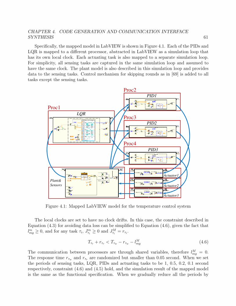
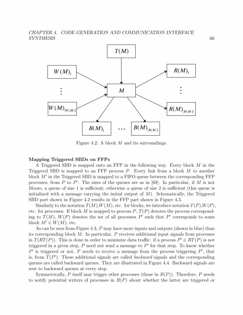
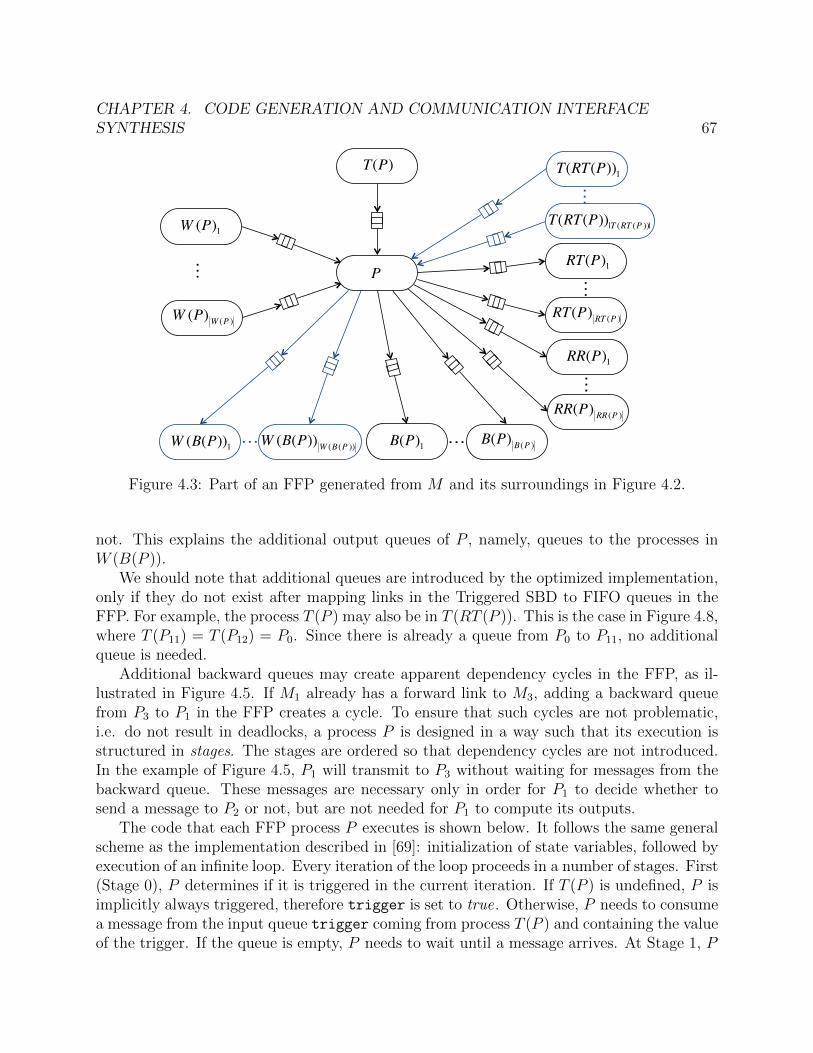
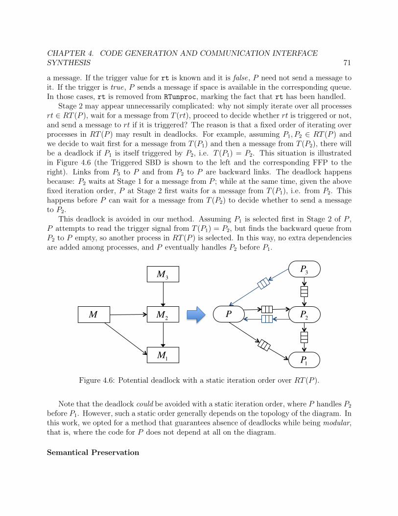
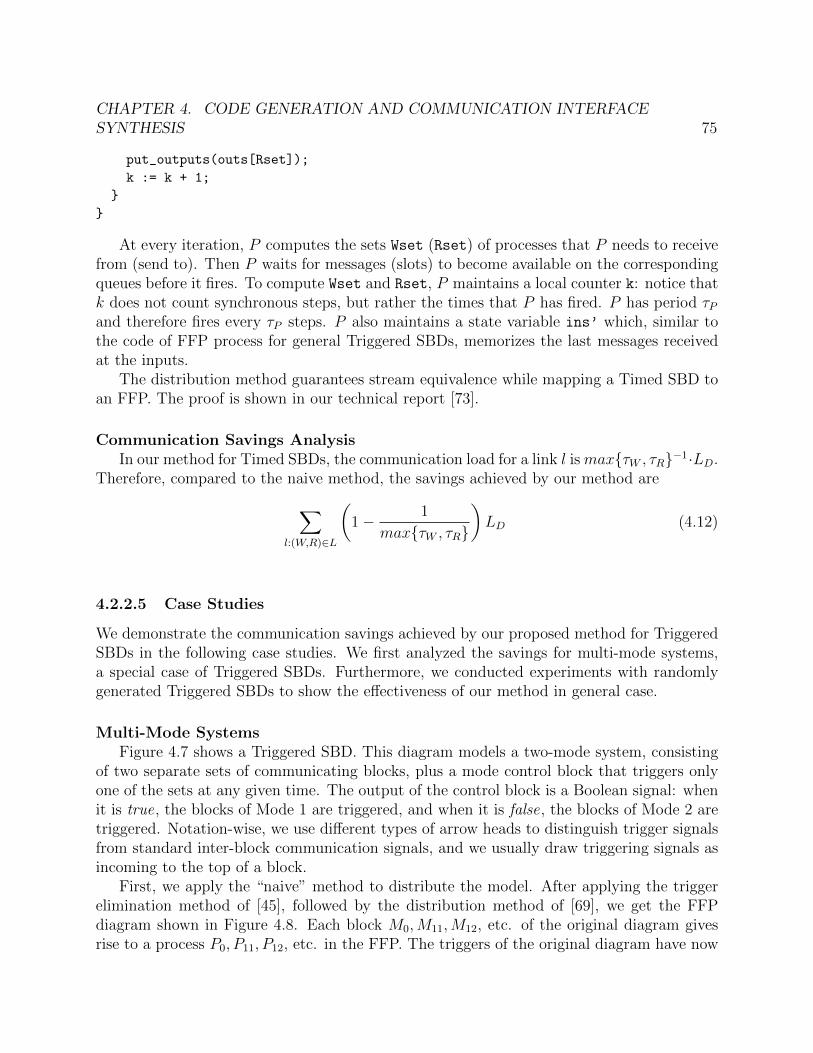
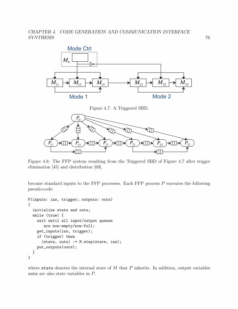
4.1 Mapped LabVIEW model for the temperature control system . . . . . . . . . . 614.2 A block M and its surroundings. . . . . . . . . . . . . . . . . . . . . . . . . . . 664.3 Part of an FFP generated from M and its surroundings in Figure 4.2. . . . . . . 674.4 Backward queue sending trigger information about P2 to P1. . . . . . . . . . . . 684.5 Avoiding deadlocks by structuring each process in stages. . . . . . . . . . . . . . 684.6 Potential deadlock with a static iteration order over RT (P ). . . . . . . . . . . . 714.7 A Triggered SBD. . . . . . . . . . . . . . . . . . . . . . . . . . . . . . . . . . . . 764.8 The FFP system resulting from the Triggered SBD of Figure 4.7 after trigger
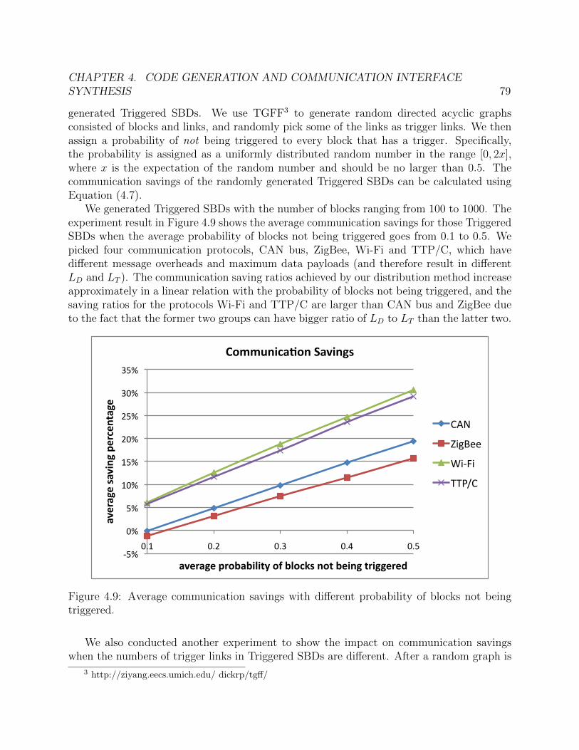
elimination [45] and distribution [69]. . . . . . . . . . . . . . . . . . . . . . . . . 764.9 Average communication savings with different probability of blocks not being
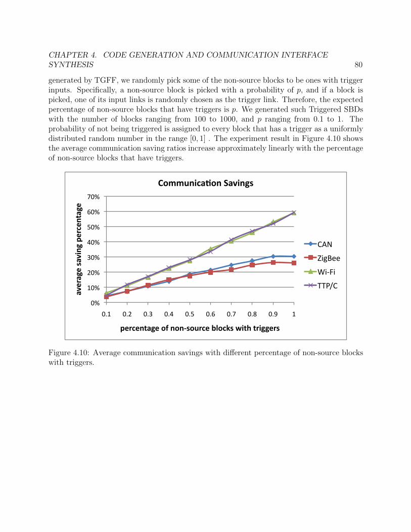
triggered. . . . . . . . . . . . . . . . . . . . . . . . . . . . . . . . . . . . . . . . 794.10 Average communication savings with different percentage of non-source blocks
I would like to first thank my advisor Prof. Alberto Sangiovanni-Vincentelli for hisguidance and support throughout my PhD study. Alberto is a great mentor with incredibleknowledge and insights on many research areas and industries. During my research, he isalways a great source of new ideas and motivations. Many of the ideas in this dissertationcame from the discussions with him. His emphasis on both rigorous theoretical foundationand potential practical applications has greatly influenced my research, and will continue toguide me in my future work. Alberto also cares deeply for his students. Over the years, hehas been very supportive in both my study and my life. For this, I will be forever grateful.
I would like to thank Prof. Sanjit Seshia and Prof. Francesco Borrelli for taking timeto review my dissertation. I also want to thank them and Prof. Jan Rabaey for being onmy qualifying exam committee. Their acute comments and suggestions help shaping andimproving this work. I had the opportunities to work with a group of wonderful researchersfrom academia and industry, and I would like to thank their help and mentorship. Theyinclude: Alessandro Pinto, Eelco Scholte, Guido Poncia, Hugo Andrade, Marco Di Natale,Mehdi Maasoumy, Michael Wetter, Philip Haves, Qi Zhu and Stavros Tripakis. In particular,Stavros Tripakis, Alessandro Pinto and Qi Zhu were heavily involved in the research workpresented in this dissertation. Their contributions are instrumental and I have learned a lotfrom them through the collaboration.
During my study at Berkeley, I have encountered many great professors and taken manyexcellent courses. In particular, I would like to thank Prof. Kurt Keutzer for readingmy Masters report and providing valuable feedback. I would like to thank Prof. AndreasKuehlmann for his logic synthesis class. It was one of the hardest courses that I took andalso one of the most satisfying courses after I completed it.
I am also fortunate to interact with a group of talented colleagues and friends. They in-clude, but not limited to: Bryan Brady, Bryan Catanzaro, Donald Chai, Satrajit Chatterjee,Minghua Chen, Jike Chong, Abhijit Davare, Douglas Densmore, Yitao Duan, Thomas Feng,Shanna-Shaye Forbes, Liangpeng Guo, Dan Holcomb, Dan Huang, Ling Huang, ShinjiroKakita, Nathan Kitchen, Yanmei Li, Wenchao Li, Chung-Wei Lin, Cong Liu, Kelvin Lwin,Mark McKelvin, Pierluigi Nuzzo, Trevor Meyerowitz, Alberto Puggelli, Kaushik Ravindran,Alena Samalatsar, Baruch Sterin, Jimmy Su, Xuening Sun, Guoqiang Wang, Lynn Wang,Zile Wei, Tobias Welp, Wei Xu, Guang Yang, Jing Yang, Haibo Zeng, Wei Zheng, FengZhou, Li Zhuang, and Jia Zou.
Last but not least, I would like to thank my parents, my husband and my daughter.Without them, I would not have accomplished my goal. My parents love me with all theirhearts, and always support me unconditionally. I will forever be in their debt. My daughterOlivia is the sweetest girl in the world and the best thing happened to me. She makes everyday exciting and bright. Even before she could speak, she was already one of my biggestsupporters. At many difficult times, she gives me the comfort and courage that I need.My husband Qi is the most important person in my life. He is so kind, caring, loving andgenerous. He is always there with me for every important decision I have made, and supports
vi
me through my ups and downs. He sits down and brainstorms with me whenever I meetdifficulties in my research and life. Now he is pursing his goals in academia, I wish him thebest.
1
Chapter 1
Introduction
Embedded systems have become ubiquitous in everyday life and are fastly growing, withwide applications in domains such as consumer electronics, automotive, aerospace, civil in-frastructure, medical devices and industrial automation. According to International DataCorporation (IDC), the market for embedded systems will double in size over the next fouryears, with estimately more than 4 billion units shipped and $2 trillion in revenue [32]. Asthe system complexity increasing rapidly in terms of both scale and functionality, many ofthe modern embedded systems are deployed on spatially-distributed and networked plat-forms. These distributed embedded systems consist of a network of embedded processors(ranging from tens to hundreds or even more) connected through wired buses or wirelesscommunication. For instance, regular modern vehicles typically employ 50 to 70 electroniccontrol units (ECUs, luxury cars may have up to 100 ECUs) and a number of buses.
Another major trend is the rapid growing of software in embedded systems, in terms ofboth amount and complexity. Using automotive domain as an example, an average car in2000 contains one million lines of code, with software taking 2% of the total value of thecar; while an average car in 2010 has 100 millions of code and software takes 13% of thecar value. It is predicted that more than 80% of car innovations in future will come fromcomputer systems, and software will become major contributor of value [66].
In addition, many complex distributed embedded systems with time and (possibly) re-liability constraints are today the result of the integration of components or subsystemsprovided by various suppliers in large quantities. For example, production quantities forautomotive subsystems are in the range of hundreds of thousands. Many avionics systems,home automation systems (HVAC controls, fire and security), and other control systems(for example elevators and industrial refrigeration systems) share similar characteristics andmodels of supply chain. All these systems are characterized by the need of a careful designand deployment of system-level functions, given the need to satisfy real-time constraints andcope with tight resource requirements because of cost constraints.
The above factors – increasing software complexity, employment of highly-distributedplatform, integration of heterogeneous components or subsystems, and tight design con-straints – propose major challenges to the design of distributed embedded systems. In cur-
CHAPTER 1. INTRODUCTION 2
rent practice, much of the design process is manual and ad-hoc, with different subsystemsdesigned in isolation. This leads to suboptimal and unreliable systems. In automotive do-main, vehicle recalls related to electronic systems have tripled in past 30 years [24], and now50% of the warranty costs are related to electronics and software [66]. In avionics domain,software complexity and integration challenge are major contributors to the production delayof Boeing 787 Dreamliner [23].
In this dissertation, we focus on the problem of implementing a given embedded applica-tion on a distributed platform with respect to a set of design objectives and constraints. Wetarget typical embedded control systems in domains such as automotive, avionics and build-ing automation, where the embedded applications are control algorithms representing thesystem functionality and the distributed platforms consist of sensors, embedded processors,actuators and communication buses. During the design process, the control algorithms thatare initially described by high-level modeling languages will be implemented as softwarecode on the distributed embedded platform. To address the design challenges mentionedabove, we propose a systematic software synthesis flow that focuses on two main aspects– integration and automation. The flow bridges the gap between a desirable design entrypoint – at a high abstraction level using model-based design tools such as Simulink [7] andModelica [6]– and the available back-end tools able to generate low-level code. The flowenables the integration of heterogeneous input models from different high-level languages,allowing the interaction between domain experts and designers of different subsystems. Italso automatically optimizes the implementation of the control algorithms on a distributedplatform by selecting computation and communication resources, and by performing codegeneration while meeting the specification. This automation of design space explorationand code synthesis makes it possible to cope with the complexity from increasing softwarecontent, highly distributed platform and tight design requirements.
1.1 A Systematic Software Synthesis Flow
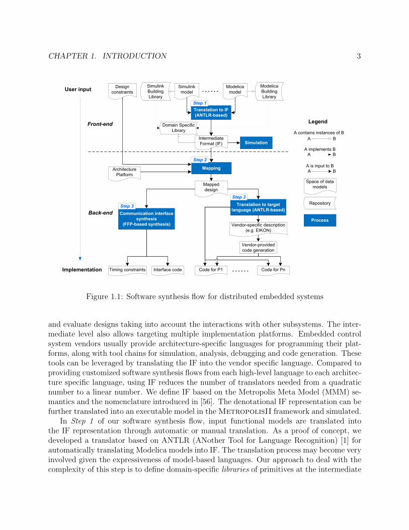
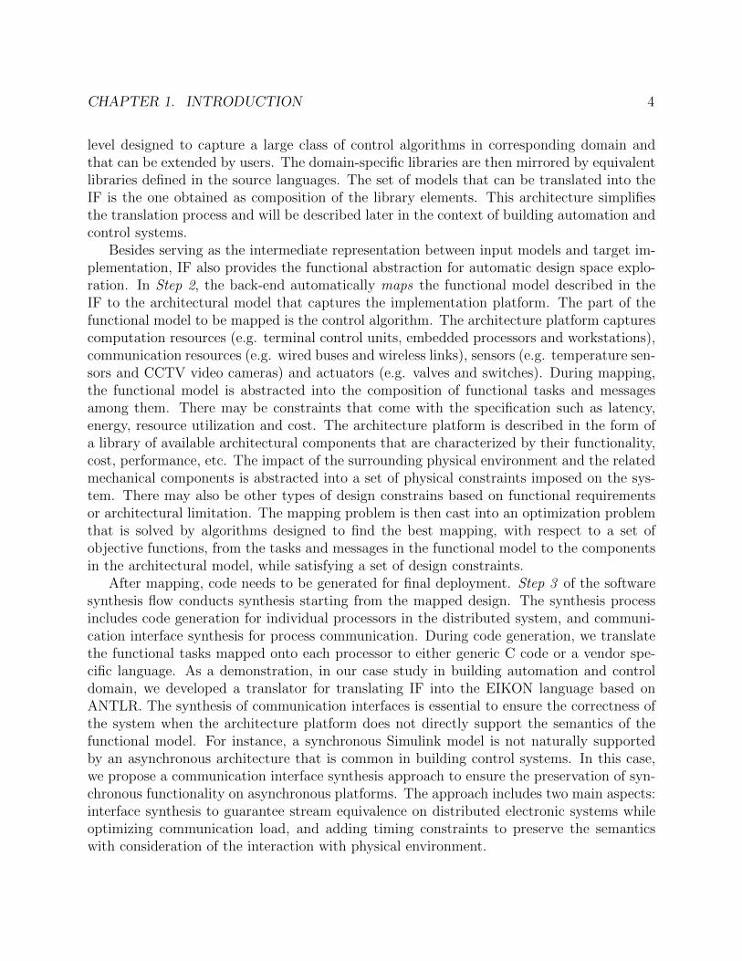
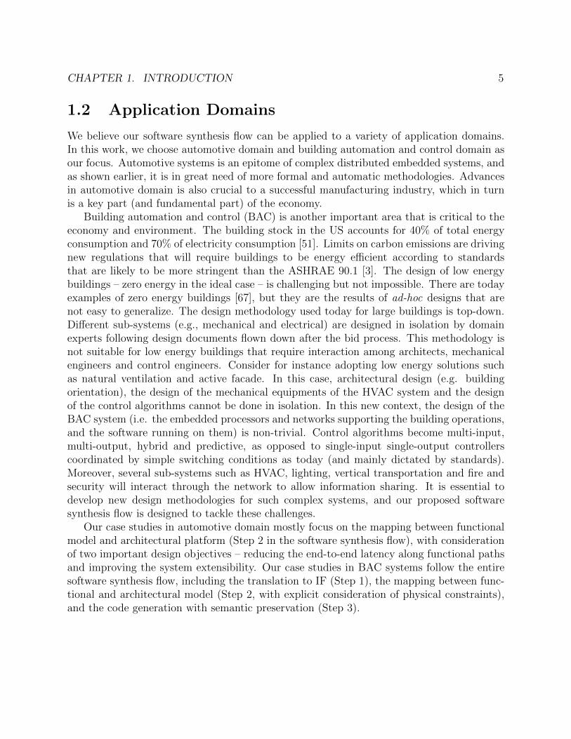
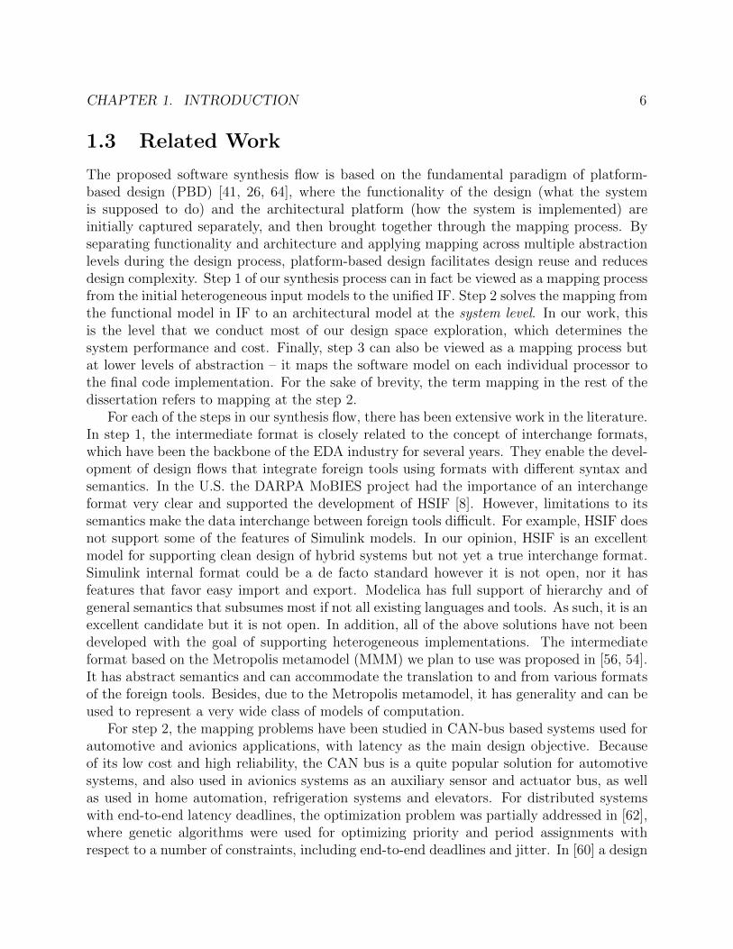
Our proposed software synthesis flow consists of a front-end and a back-end, as shown inFigure 1.1. The front-end is used to model the system including the control algorithms andthe behavior of the environment. The back-end includes a set of tools that, given the spec-ification of the control algorithms and a set of available computation and communicationresources, automatically refines the specification into an optimal distributed implementation.The front-end and the back-end exchange models using an intermediate format (IF). Theintroduction of this intermediate layer is essential for the integration of heterogeneous inputs,the leverage of back-end tools, and automatic design space exploration. It enables buildinga software synthesis flow that is general with respect to the user input (e.g. Simulink andModelica), and to the output implementation code (e.g. C and domain-specific languagesuch as EIKON [5] for building automation and control). Using an IF, pieces of the inputspecification expressed in different languages can be composed. This feature will hopefullyfoster collaboration among experts in different disciplines by allowing them exchange models
CHAPTER 1. INTRODUCTION 3
Simulink
model
Modelica
model
Simulink
Building
Library
Modelica
Building
Library
Translation to IF
(ANTLR-based)
Intermediate
Format (IF)
Domain Specific
Library
MappingArchitecture
Platform
Mapped
design
Communication interface
synthesis
(FFP-based synthesis)
Code for PnCode for P1
Translation to target
language (ANTLR-based)
Vendor-specific description
(e.g. EIKON)
Vendor-provided
code generation
Interface code
Space of data
models
Repository
Process
A B
A contains instances of B
A implements BA B
A B
A is input to B
Legend
User input
Implementation
Step 2
Step 3
Step 1
Step 3
Design
constraints
Simulation
Front-end
Back-end
Timing constraints
Figure 1.1: Software synthesis flow for distributed embedded systems
and evaluate designs taking into account the interactions with other subsystems. The inter-mediate level also allows targeting multiple implementation platforms. Embedded controlsystem vendors usually provide architecture-specific languages for programming their plat-forms, along with tool chains for simulation, analysis, debugging and code generation. Thesetools can be leveraged by translating the IF into the vendor specific language. Compared toproviding customized software synthesis flows from each high-level language to each architec-ture specific language, using IF reduces the number of translators needed from a quadraticnumber to a linear number. We define IF based on the Metropolis Meta Model (MMM) se-mantics and the nomenclature introduced in [56]. The denotational IF representation can befurther translated into an executable model in the MetropolisII framework and simulated.
In Step 1 of our software synthesis flow, input functional models are translated intothe IF representation through automatic or manual translation. As a proof of concept, wedeveloped a translator based on ANTLR (ANother Tool for Language Recognition) [1] forautomatically translating Modelica models into IF. The translation process may become veryinvolved given the expressiveness of model-based languages. Our approach to deal with thecomplexity of this step is to define domain-specific libraries of primitives at the intermediate
CHAPTER 1. INTRODUCTION 4
level designed to capture a large class of control algorithms in corresponding domain andthat can be extended by users. The domain-specific libraries are then mirrored by equivalentlibraries defined in the source languages. The set of models that can be translated into theIF is the one obtained as composition of the library elements. This architecture simplifiesthe translation process and will be described later in the context of building automation andcontrol systems.
Besides serving as the intermediate representation between input models and target im-plementation, IF also provides the functional abstraction for automatic design space explo-ration. In Step 2, the back-end automatically maps the functional model described in theIF to the architectural model that captures the implementation platform. The part of thefunctional model to be mapped is the control algorithm. The architecture platform capturescomputation resources (e.g. terminal control units, embedded processors and workstations),communication resources (e.g. wired buses and wireless links), sensors (e.g. temperature sen-sors and CCTV video cameras) and actuators (e.g. valves and switches). During mapping,the functional model is abstracted into the composition of functional tasks and messagesamong them. There may be constraints that come with the specification such as latency,energy, resource utilization and cost. The architecture platform is described in the form ofa library of available architectural components that are characterized by their functionality,cost, performance, etc. The impact of the surrounding physical environment and the relatedmechanical components is abstracted into a set of physical constraints imposed on the sys-tem. There may also be other types of design constrains based on functional requirementsor architectural limitation. The mapping problem is then cast into an optimization problemthat is solved by algorithms designed to find the best mapping, with respect to a set ofobjective functions, from the tasks and messages in the functional model to the componentsin the architectural model, while satisfying a set of design constraints.
After mapping, code needs to be generated for final deployment. Step 3 of the softwaresynthesis flow conducts synthesis starting from the mapped design. The synthesis processincludes code generation for individual processors in the distributed system, and communi-cation interface synthesis for process communication. During code generation, we translatethe functional tasks mapped onto each processor to either generic C code or a vendor spe-cific language. As a demonstration, in our case study in building automation and controldomain, we developed a translator for translating IF into the EIKON language based onANTLR. The synthesis of communication interfaces is essential to ensure the correctness ofthe system when the architecture platform does not directly support the semantics of thefunctional model. For instance, a synchronous Simulink model is not naturally supportedby an asynchronous architecture that is common in building control systems. In this case,we propose a communication interface synthesis approach to ensure the preservation of syn-chronous functionality on asynchronous platforms. The approach includes two main aspects:interface synthesis to guarantee stream equivalence on distributed electronic systems whileoptimizing communication load, and adding timing constraints to preserve the semanticswith consideration of the interaction with physical environment.
CHAPTER 1. INTRODUCTION 5
1.2 Application Domains
We believe our software synthesis flow can be applied to a variety of application domains.In this work, we choose automotive domain and building automation and control domain asour focus. Automotive systems is an epitome of complex distributed embedded systems, andas shown earlier, it is in great need of more formal and automatic methodologies. Advancesin automotive domain is also crucial to a successful manufacturing industry, which in turnis a key part (and fundamental part) of the economy.
Building automation and control (BAC) is another important area that is critical to theeconomy and environment. The building stock in the US accounts for 40% of total energyconsumption and 70% of electricity consumption [51]. Limits on carbon emissions are drivingnew regulations that will require buildings to be energy efficient according to standardsthat are likely to be more stringent than the ASHRAE 90.1 [3]. The design of low energybuildings – zero energy in the ideal case – is challenging but not impossible. There are todayexamples of zero energy buildings [67], but they are the results of ad-hoc designs that arenot easy to generalize. The design methodology used today for large buildings is top-down.Different sub-systems (e.g., mechanical and electrical) are designed in isolation by domainexperts following design documents flown down after the bid process. This methodology isnot suitable for low energy buildings that require interaction among architects, mechanicalengineers and control engineers. Consider for instance adopting low energy solutions suchas natural ventilation and active facade. In this case, architectural design (e.g. buildingorientation), the design of the mechanical equipments of the HVAC system and the designof the control algorithms cannot be done in isolation. In this new context, the design of theBAC system (i.e. the embedded processors and networks supporting the building operations,and the software running on them) is non-trivial. Control algorithms become multi-input,multi-output, hybrid and predictive, as opposed to single-input single-output controllerscoordinated by simple switching conditions as today (and mainly dictated by standards).Moreover, several sub-systems such as HVAC, lighting, vertical transportation and fire andsecurity will interact through the network to allow information sharing. It is essential todevelop new design methodologies for such complex systems, and our proposed softwaresynthesis flow is designed to tackle these challenges.
Our case studies in automotive domain mostly focus on the mapping between functionalmodel and architectural platform (Step 2 in the software synthesis flow), with considerationof two important design objectives – reducing the end-to-end latency along functional pathsand improving the system extensibility. Our case studies in BAC systems follow the entiresoftware synthesis flow, including the translation to IF (Step 1), the mapping between func-tional and architectural model (Step 2, with explicit consideration of physical constraints),and the code generation with semantic preservation (Step 3).
CHAPTER 1. INTRODUCTION 6
1.3 Related Work
The proposed software synthesis flow is based on the fundamental paradigm of platform-based design (PBD) [41, 26, 64], where the functionality of the design (what the systemis supposed to do) and the architectural platform (how the system is implemented) areinitially captured separately, and then brought together through the mapping process. Byseparating functionality and architecture and applying mapping across multiple abstractionlevels during the design process, platform-based design facilitates design reuse and reducesdesign complexity. Step 1 of our synthesis process can in fact be viewed as a mapping processfrom the initial heterogeneous input models to the unified IF. Step 2 solves the mapping fromthe functional model in IF to an architectural model at the system level. In our work, thisis the level that we conduct most of our design space exploration, which determines thesystem performance and cost. Finally, step 3 can also be viewed as a mapping process butat lower levels of abstraction – it maps the software model on each individual processor tothe final code implementation. For the sake of brevity, the term mapping in the rest of thedissertation refers to mapping at the step 2.
For each of the steps in our synthesis flow, there has been extensive work in the literature.In step 1, the intermediate format is closely related to the concept of interchange formats,which have been the backbone of the EDA industry for several years. They enable the devel-opment of design flows that integrate foreign tools using formats with different syntax andsemantics. In the U.S. the DARPA MoBIES project had the importance of an interchangeformat very clear and supported the development of HSIF [8]. However, limitations to itssemantics make the data interchange between foreign tools difficult. For example, HSIF doesnot support some of the features of Simulink models. In our opinion, HSIF is an excellentmodel for supporting clean design of hybrid systems but not yet a true interchange format.Simulink internal format could be a de facto standard however it is not open, nor it hasfeatures that favor easy import and export. Modelica has full support of hierarchy and ofgeneral semantics that subsumes most if not all existing languages and tools. As such, it is anexcellent candidate but it is not open. In addition, all of the above solutions have not beendeveloped with the goal of supporting heterogeneous implementations. The intermediateformat based on the Metropolis metamodel (MMM) we plan to use was proposed in [56, 54].It has abstract semantics and can accommodate the translation to and from various formatsof the foreign tools. Besides, due to the Metropolis metamodel, it has generality and can beused to represent a very wide class of models of computation.
For step 2, the mapping problems have been studied in CAN-bus based systems used forautomotive and avionics applications, with latency as the main design objective. Becauseof its low cost and high reliability, the CAN bus is a quite popular solution for automotivesystems, and also used in avionics systems as an auxiliary sensor and actuator bus, as wellas used in home automation, refrigeration systems and elevators. For distributed systemswith end-to-end latency deadlines, the optimization problem was partially addressed in [62],where genetic algorithms were used for optimizing priority and period assignments withrespect to a number of constraints, including end-to-end deadlines and jitter. In [60] a design
CHAPTER 1. INTRODUCTION 7
optimization heuristics-based algorithm for mixed time-triggered and event-triggered systemswas proposed. The algorithm, however, assumed that nodes are synchronized. In [48], aSAT-based approach for task and message placement was proposed. The method providedoptimal solutions to the placement and priority assignment. However, it did not considersignal packing. In [33], task and message periods are explored in an algorithm based ongeometric programming to satisfy latency constraints. In [50], the trade-offs between thepurely periodic and the data-driven activation models are leveraged to meet the latencyrequirements of distributed vehicle functions. In [75, 79], task allocation, signal packingand message allocation, as well as task and message priority are explored to optimize theend-to-end path latencies.
In our work for automotive systems, besides the traditional design objectives such aslatency and utilization, we also optimize the metric of task extensibility, which measureshow much the task execution time may be increased without violating design constraints.The literature on extensibility is rich. Sensitivity analysis was studied for priority-basedscheduled distributed systems [62], with respect to end-to-end deadlines. The evaluation ofextensibility with respect to changes in task execution times, when the system is character-ized by end-to-end deadlines, was studied in [74]. The notion of robustness under reducedsystem load was defined and analyzed in [49], for both preemptive and non-preemptive sys-tems. The paper highlights possible anomalies (increased response times for shorter taskexecution times) that would make evaluation of extensibility quite complex. These papersdo not explicitly address system optimization. Task allocation, priorities, and message con-figuration, are assumed as given. Also, it is worth mentioning that time anomalies such asthose in [49] and other described in several other papers on multiprocessor and distributedscheduling do not occur for the scheduling and information propagation model we consider.This is because we assume local scheduling by preemption, the passing of information byperiodic sampling and the periodic (not event-based) activation of each task and message.This decouples the scheduling of each task and message from predecessors and successors aswell as from scheduling on other resources and avoids anomalies. In [15], task allocation andpriority assignment are defined with the purpose of optimizing the extensibility with respectto changes in task computation times. The proposed solution is based on simulated anneal-ing, and the maximum amount of change that can be tolerated in the task execution timeswithout missing end-to-end deadlines is computed by scaling all task times by a constantfactor. A model of event-based activation for task and messages is assumed. In [37, 39, 38],a generalized definition of extensibility on multiple dimensions (including changes in theexecution times of tasks as in our definition, but also period speed-ups and possibly othermetrics) is presented. A randomized optimization procedure based on a genetic algorithmis proposed to solve the optimization problem. These papers focus on the multi-parameterPareto optimization, and how to discriminate the set of optimal solutions. The main limi-tation of this approach is complexity and expected running time of the genetic optimizationalgorithm. In addition, randomized optimization algorithms are difficult to control and giveno guarantee on the quality of the obtained solution. Indeed, in the cited papers, the useof genetic optimization is only demonstrated for small sample cases. In [39], the experi-
CHAPTER 1. INTRODUCTION 8
ments show the optimization of a sample system with 9 tasks and 6 messages. The searchspace consists of the priority assignments on all processors and on the interconnecting bus.Hence, task allocation (possibly the most complex step) and signal to message packing arenot subject to optimization. Yet, a complete robustness optimization takes approximately900 and 3000 seconds for the two-dimensional and three-dimensional case, respectively. Ingeneral, the computation time required by randomized optimization approaches for largeand complex problems may easily be an issue. In [37] a larger set of “20 tasks and message”is considered, with only priority assignment subject to optimization. These results albeitimportant in their own right, exhibit a running time that is clearly infeasible for an effectivedesign space exploration. This observation motivated us to develop a two-stage “determin-istic” algorithm that has running times over an order of magnitude faster than the onesproposed so far in the literature, as explained later in Chapter 3.
For step 3, the main challenge is to preserve the semantics during code generation withminimal cost. There is a large body of research on distribution of synchronous models,and in particular synchronous languages [20]. For instance, a dynamic buffering protocol isproposed in [65] for preservation of semantics when distributing a synchronous model to mul-tiple tasks running under preemptive scheduling. The buffering protocol can be used for intertask communication inside a processor. A mechanism to distribute a synchronous model toLoosely Time Triggered Architecture(LTTA) is proposed and proved to guarantee semanticspreservation in [69]. Other than synchronous programs, there has also been research on codegeneration for other models of computation. Software synthesis method proposed in [13]focuses on distributing a global asynchronous local synchronous (GALS) network of CFSMsand proposes a method to generate RTOS for communication among CFSMs. In [80], a gen-eral execution strategy is defined for executing discrete event (DE) semantics on distributedplatform, by ensuring each actor processes input events in time-stamp order.
In our work, we focus on code generation for synchronous models. We leverage the workfrom [69], which defines an intermediate layer called Finite FIFO Platform (FFP) to facilitatethe distribution of synchronous models on LTTA platforms. The FFP platform makes noassumptions on clock synchronization. This has the advantage of providing implementationsthat are robust to various types of timing uncertainties such as clock drifts and networkdelays. Similar techniques are used in the design of digital circuits, in particular, latency-insensitive or elastic circuits [27, 28]. On the other hand, knowledge about the timingcharacteristics of the execution platform may sometimes be available, e.g. bounds on clockdrifts and network delays. Implementation techniques that leverage such type of knowledgecan be found in [63, 29, 17]. There are also studies that target synchronous distributedexecution platforms such as the Time-Triggered Architecture [43]. In that case, one of themain challenges is to synthesize time-triggered communication schedules so that semanticsis preserved [30]. We further develop an approach to optimize the communication loadwhile conducting code generation for a particular set of synchronous models – the TriggeredSynchronous Block Diagrams (SBDs). The model of Triggered SBDs is directly inspired bytools such as Simulink and SCADE. SCADE can be seen as a subclass of Lustre [31]. Sincewe only target a restricted class of synchronous models, we avoid many of the difficulties
CHAPTER 1. INTRODUCTION 9
encountered when considering more general models, such as the full Lustre, Signal or Esterelsynchronous languages, for which there exists a wealth of techniques [36, 18, 63, 61, 16].Furthermore, for this communication optimization work, we assume a one-to-one mappingbetween blocks of the synchronous model and processes of the distributed architecture. Thissimplifies the problem and allows focusing on semantical preservation. How to allocatefunctional blocks to processes is an important and difficult problem in embedded controlsystems, that often involves multi-criteria optimization and tradeoffs, e.g. see [68, 59, 58, 75].
Compared to the above related work, this dissertation makes novel contributions in thefollowing areas.
• We propose a complete software synthesis flow for distributed embedded systems, andapply it to the building automation and control systems. Starting from a high levelmodel-based input specification, our flow generates a unified IF representation for facil-itating the following synthesis steps, conducts design space exploration through map-ping algorithm, and performs code generation on distributed platforms with semanticpreservation and communication optimization. As far as we know, this is the firstattempt in developing a synthesis flow from model-based specification to embeddedimplementation for building control systems.
• We develop an automatic translator from Modelica input model to IF at the front-endand an automatic translator from IF to EIKON embedded language at the back-end.Both translators are implemented using the ANTLR framework. The mapping stepand the code generation step are automated by algorithms. Together they demonstrate,as a proof-of-concept, an automated flow from input to implementation.
• In the mapping step, we extend the traditional concept of mapping a given functionalmodel to a given architectural platform to include the exploration of the architecturalplatform. This in principle provides more optimization opportunities. We also definea novel metric and algorithm for optimizing the system extensibility in mapping.
• In the code generation step, we extend the previous work on semantic-preserving syn-thesis for LTTA to include the consideration of physical environment (therefore addi-tional timing constraints) and the optimization of communication load for TriggeredSBDs.
• We leverage the MetropolisII framework as an executable IF for simulation-basedanalysis and validation, in particular we apply it to a heterogeneous input model forbuilding control systems.
In rest of the dissertation, the three steps in the software synthesis flow will be introducedin Chapter 2, Chapter 3 and Chapter 4, respectively. Case studies are presented in each ofthe chapters, including temperature control systems in building automation and control aswell as automotive safety and control systems . Chapter 5 concludes our current work anddiscusses the future directions.
10
Chapter 2
Intermediate Format
In Step 1 of our software synthesis flow, models capturing the specification of the controlalgorithms and of the environment are translated into an intermediate format (IF) thatis defined to facilitate the other steps in the synthesis flow, namely mapping and codegeneration. Because the type of specifications that we are interested in are in general hybridsystems [46] with multiple semantics, the IF representation may become very complex [56,54], and thus not directly usable in the mapping and code generation steps. In the envisionedfinal form of our design method, IF will be manipulated and partitioned to make the mappingand code generation steps effective. In our work that is a first step towards the ideal scenario,we restrict the IF to dataflow semantics [44] which is amenable to efficient mapping and codegeneration. We base our IF definition on the Metropolis Meta Model (MMM) semanticsand retain the nomenclature introduced in [56] as we plan to extend this work to moregeneral intermediate representations. In particular, processes (also called actors) are thebasic entities for specification. They are categorized into continuous processes and discreteprocesses. Each process is defined by a set of parameters, ports and equations. Parameters areset for configuring the process. Ports constitute the communication interface of the processand can be either input or output port. Equations capture the behavior of the process in theform of an input-output function. Multiple processes may be connected through channels toform a netlist at the higher level and eventually build the entire system. During execution,the equations in the processes are executed according to an order determined by an equationmanager (EM) that is local to the process. The set of processes in the system is scheduledby an equation resolve manager (ERM).
2.1 IF Translation and IF library
The translation process may be done manually or through automatic translators. We devel-oped a translator for Modelica based on the ANTLR framework, a parser generator that usesLL(*) parsing. We chose ANTLR because it provides comprehensive support and consistentsyntax for specifying lexers, parsers and tree parsers, and supports generating code in com-
CHAPTER 2. INTERMEDIATE FORMAT 11
mon languages such as C, Java, Ada and Objective-C. The translator we developed includesa lexer and a parser for parsing the Modelica language (currently without full support ofinheritance and algorithm), and a code generator for generating IF. The following samplecode snippet shows part of the ANTLR input for generating the lexer, parser and generatorfor the process entity.
Domain specific libraries can be used to enable fast translations to (and from) IF. As anexample, we define a domain specific IF library for HVAC control systems in buildings, andwe export the library to different specification languages. We reviewed 71 HVAC-relatedcomponent models in the GPL language from Johnson Controls [9], 70 in Automated LogicEIKON language [10], 42 in Honeywell Spyder [11], and 59 in the HVAC library defined bythe Lawrence Berkeley National Laboratory [70]. Based on these information, we defined aset of basic components used in HVAC control systems and the corresponding processes inthe IF, including:
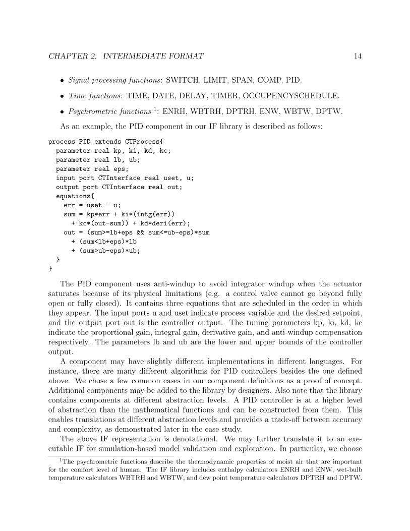
As an example, the PID component in our IF library is described as follows:
process PID extends CTProcess{
parameter real kp, ki, kd, kc;
parameter real lb, ub;
parameter real eps;
input port CTInterface real uset, u;
output port CTInterface real out;
equations{
err = uset - u;
sum = kp*err + ki*(intg(err))
+ kc*(out-sum)) + kd*deri(err);
out = (sum>=lb+eps && sum<=ub-eps)*sum
+ (sum<lb+eps)*lb
+ (sum>ub-eps)*ub;
}
}
The PID component uses anti-windup to avoid integrator windup when the actuatorsaturates because of its physical limitations (e.g. a control valve cannot go beyond fullyopen or fully closed). It contains three equations that are scheduled in the order in whichthey appear. The input ports u and uset indicate process variable and the desired setpoint,and the output port out is the controller output. The tuning parameters kp, ki, kd, kcindicate the proportional gain, integral gain, derivative gain, and anti-windup compensationrespectively. The parameters lb and ub are the lower and upper bounds of the controlleroutput.
A component may have slightly different implementations in different languages. Forinstance, there are many different algorithms for PID controllers besides the one definedabove. We chose a few common cases in our component definitions as a proof of concept.Additional components may be added to the library by designers. Also note that the librarycontains components at different abstraction levels. A PID controller is at a higher levelof abstraction than the mathematical functions and can be constructed from them. Thisenables translations at different abstraction levels and provides a trade-off between accuracyand complexity, as demonstrated later in the case study.
The above IF representation is denotational. We may further translate it to an exe-cutable IF for simulation-based model validation and exploration. In particular, we choose
1The psychrometric functions describe the thermodynamic properties of moist air that are importantfor the comfort level of human. The IF library includes enthalpy calculators ENRH and ENW, wet-bulbtemperature calculators WBTRH and WBTW, and dew point temperature calculators DPTRH and DPTW.
CHAPTER 2. INTERMEDIATE FORMAT 15
the MetropolisII framework [14] for modeling and simulating the executable IF, becauseits semantics also derives from the Metropolis Meta Model (same as the denotational IF)and it provides strong support on modeling heterogeneous systems. The translation fromdenotational IF to MetropolisII model is straightforward because of the similarity of theirsemantics. Processes in IF are translated to components in MetropolisII, with equationstranslated to constraints. The ERM and EMs in IF are translated to constraint solversand schedulers, which govern the resolution and scheduling of constraints in a three-phaseexecution semantics.
2.2 Case Study
We conducted a case study on a room temperature control system example to illustrate theapplication of our software synthesis flow in building automation and control systems. Thisexample will be used throughout the dissertation for each of the three steps in the flow. Inthis chapter, we will first show how the design input, a heterogeneous functional model ofthe temperature control system, is translated into an IF representation.
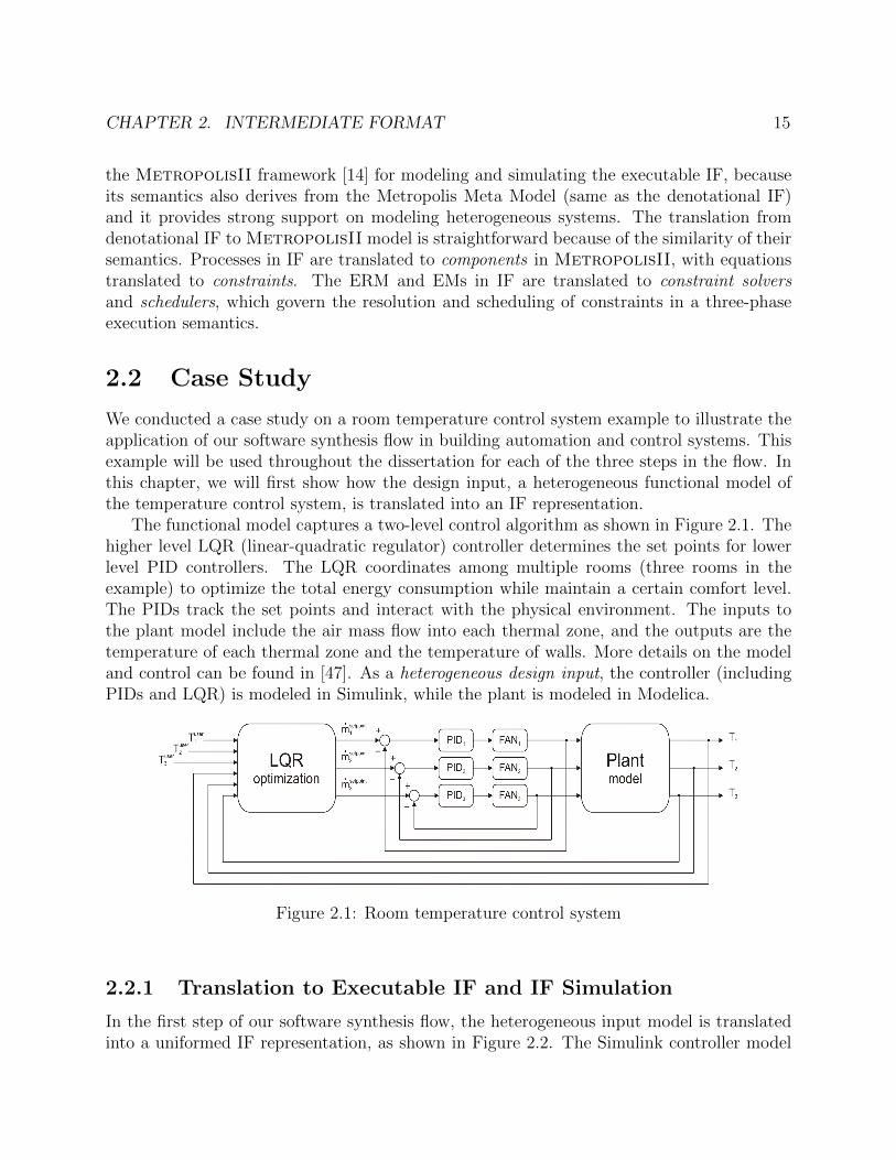
The functional model captures a two-level control algorithm as shown in Figure 2.1. Thehigher level LQR (linear-quadratic regulator) controller determines the set points for lowerlevel PID controllers. The LQR coordinates among multiple rooms (three rooms in theexample) to optimize the total energy consumption while maintain a certain comfort level.The PIDs track the set points and interact with the physical environment. The inputs tothe plant model include the air mass flow into each thermal zone, and the outputs are thetemperature of each thermal zone and the temperature of walls. More details on the modeland control can be found in [47]. As a heterogeneous design input, the controller (includingPIDs and LQR) is modeled in Simulink, while the plant is modeled in Modelica.
Figure 2.1: Room temperature control system
2.2.1 Translation to Executable IF and IF Simulation
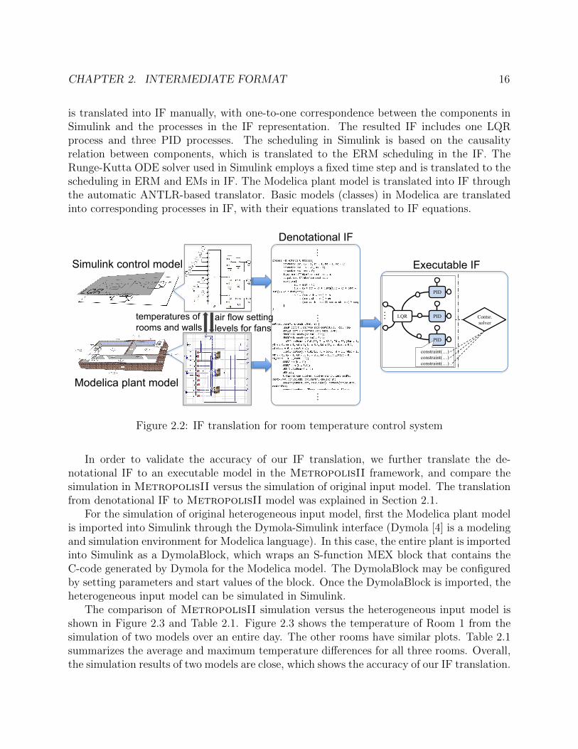
In the first step of our software synthesis flow, the heterogeneous input model is translatedinto a uniformed IF representation, as shown in Figure 2.2. The Simulink controller model
CHAPTER 2. INTERMEDIATE FORMAT 16
is translated into IF manually, with one-to-one correspondence between the components inSimulink and the processes in the IF representation. The resulted IF includes one LQRprocess and three PID processes. The scheduling in Simulink is based on the causalityrelation between components, which is translated to the ERM scheduling in the IF. TheRunge-Kutta ODE solver used in Simulink employs a fixed time step and is translated to thescheduling in ERM and EMs in IF. The Modelica plant model is translated into IF throughthe automatic ANTLR-based translator. Basic models (classes) in Modelica are translatedinto corresponding processes in IF, with their equations translated to IF equations.
Modelica plant model
Simulink control model
temperatures of rooms and walls
air flow setting levels for fans
Denotational IF
Executable IF …
…
…
PID
PID
PID
LQR
constraint(…) constraint(…) constraint(…)
… Contsr.
solver
Figure 2.2: IF translation for room temperature control system
In order to validate the accuracy of our IF translation, we further translate the de-notational IF to an executable model in the MetropolisII framework, and compare thesimulation in MetropolisII versus the simulation of original input model. The translationfrom denotational IF to MetropolisII model was explained in Section 2.1.
For the simulation of original heterogeneous input model, first the Modelica plant modelis imported into Simulink through the Dymola-Simulink interface (Dymola [4] is a modelingand simulation environment for Modelica language). In this case, the entire plant is importedinto Simulink as a DymolaBlock, which wraps an S-function MEX block that contains theC-code generated by Dymola for the Modelica model. The DymolaBlock may be configuredby setting parameters and start values of the block. Once the DymolaBlock is imported, theheterogeneous input model can be simulated in Simulink.
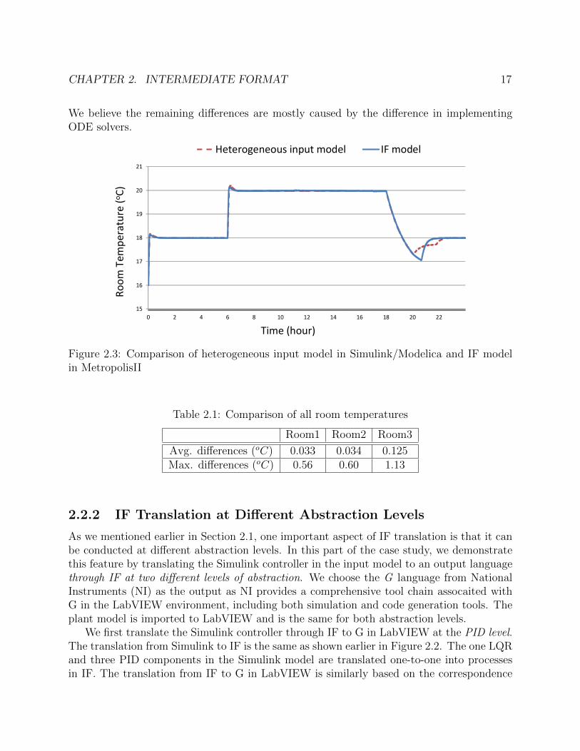
The comparison of MetropolisII simulation versus the heterogeneous input model isshown in Figure 2.3 and Table 2.1. Figure 2.3 shows the temperature of Room 1 from thesimulation of two models over an entire day. The other rooms have similar plots. Table 2.1summarizes the average and maximum temperature differences for all three rooms. Overall,the simulation results of two models are close, which shows the accuracy of our IF translation.
CHAPTER 2. INTERMEDIATE FORMAT 17
We believe the remaining differences are mostly caused by the difference in implementingODE solvers.
15
16
17
18
19
20
21
0 2 4 6 8 10 12 14 16 18 20 22
Heterogeneous input model IF model
Room
Tem
pera
ture
(o C)
Time (hour)
Figure 2.3: Comparison of heterogeneous input model in Simulink/Modelica and IF modelin MetropolisII
2.2.2 IF Translation at Different Abstraction Levels
As we mentioned earlier in Section 2.1, one important aspect of IF translation is that it canbe conducted at different abstraction levels. In this part of the case study, we demonstratethis feature by translating the Simulink controller in the input model to an output languagethrough IF at two different levels of abstraction. We choose the G language from NationalInstruments (NI) as the output as NI provides a comprehensive tool chain assocaited withG in the LabVIEW environment, including both simulation and code generation tools. Theplant model is imported to LabVIEW and is the same for both abstraction levels.
We first translate the Simulink controller through IF to G in LabVIEW at the PID level.The translation from Simulink to IF is the same as shown earlier in Figure 2.2. The one LQRand three PID components in the Simulink model are translated one-to-one into processesin IF. The translation from IF to G in LabVIEW is similarly based on the correspondence
CHAPTER 2. INTERMEDIATE FORMAT 18
at the component level. As mentioned before, the scheduling in Simulink for the dataflowtype semantics is based on the causality relation between components. This is translated toERM scheduling in IF, and further translated to the component scheduling in LabVIEW,which is also based on causality relations. The Runge-Kutta ODE solver used in Simulink istranslated to ERM and EM scheduling in IF, and then translated to the Runge-Kutta solveravailable in LabVIEW.
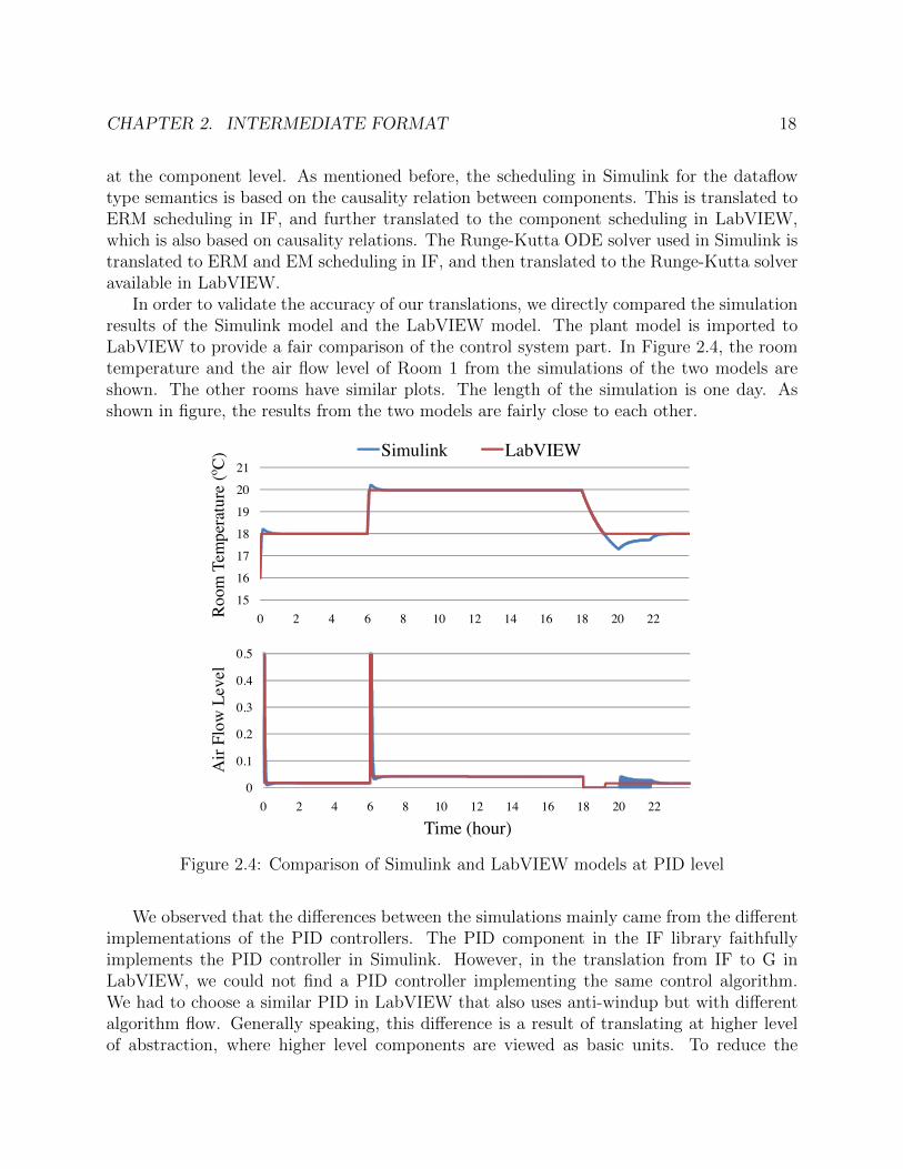
In order to validate the accuracy of our translations, we directly compared the simulationresults of the Simulink model and the LabVIEW model. The plant model is imported toLabVIEW to provide a fair comparison of the control system part. In Figure 2.4, the roomtemperature and the air flow level of Room 1 from the simulations of the two models areshown. The other rooms have similar plots. The length of the simulation is one day. Asshown in figure, the results from the two models are fairly close to each other.
Room
Tem
pera
ture
(o C)
Air
Flow
Lev
el
Time (hour)
15
16
17
18
19
20
21
0 2 4 6 8 10 12 14 16 18 20 22
Simulink LabVIEW
0
0.1
0.2
0.3
0.4
0.5
0 2 4 6 8 10 12 14 16 18 20 22
Figure 2.4: Comparison of Simulink and LabVIEW models at PID level
We observed that the differences between the simulations mainly came from the differentimplementations of the PID controllers. The PID component in the IF library faithfullyimplements the PID controller in Simulink. However, in the translation from IF to G inLabVIEW, we could not find a PID controller implementing the same control algorithm.We had to choose a similar PID in LabVIEW that also uses anti-windup but with differentalgorithm flow. Generally speaking, this difference is a result of translating at higher levelof abstraction, where higher level components are viewed as basic units. To reduce the
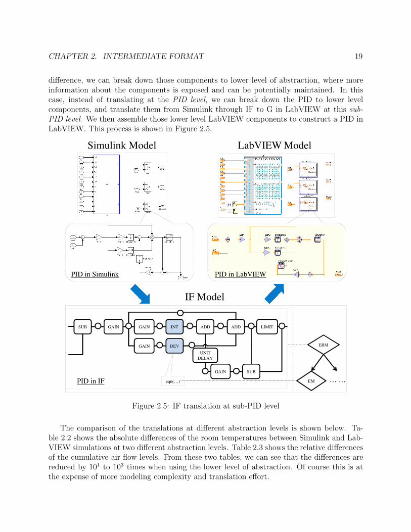
CHAPTER 2. INTERMEDIATE FORMAT 19
difference, we can break down those components to lower level of abstraction, where moreinformation about the components is exposed and can be potentially maintained. In thiscase, instead of translating at the PID level, we can break down the PID to lower levelcomponents, and translate them from Simulink through IF to G in LabVIEW at this sub-PID level. We then assemble those lower level LabVIEW components to construct a PID inLabVIEW. This process is shown in Figure 2.5.
Simulink Model
IF Model
ERM
EM … …
SUB GAIN GAIN
GAIN
INT
DEV
ADD ADD
GAIN SUB
LIMIT
eqn(…)
UNITDELAY
PID in Simulink PID in LabVIEW
PID in IF
LabVIEW Model
Figure 2.5: IF translation at sub-PID level
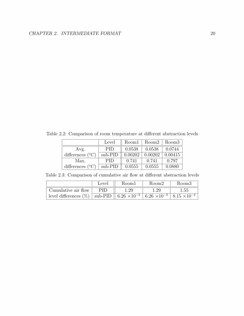
The comparison of the translations at different abstraction levels is shown below. Ta-ble 2.2 shows the absolute differences of the room temperatures between Simulink and Lab-VIEW simulations at two different abstraction levels. Table 2.3 shows the relative differencesof the cumulative air flow levels. From these two tables, we can see that the differences arereduced by 101 to 103 times when using the lower level of abstraction. Of course this is atthe expense of more modeling complexity and translation effort.
CHAPTER 2. INTERMEDIATE FORMAT 20
Table 2.2: Comparison of room temperature at different abstraction levels
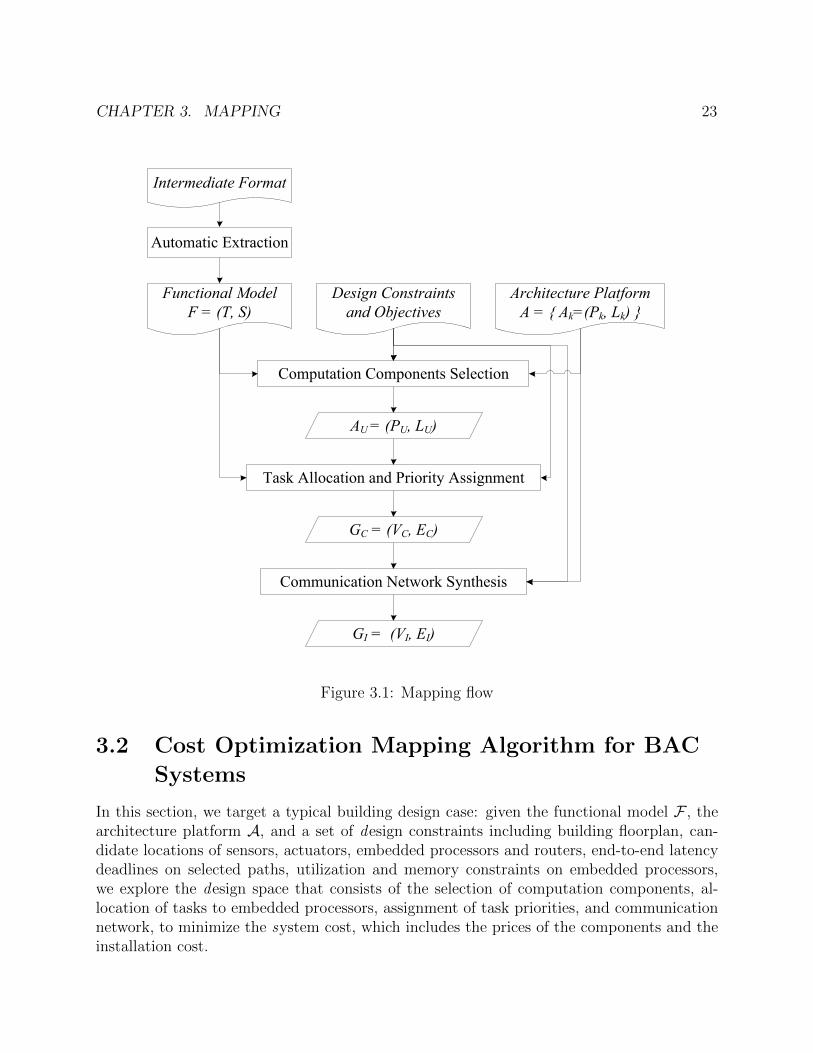
In Step 2 of the software synthesis flow, mapping is conducted to explore the design space,including the selection of computation resources, the allocation of control functions onto pro-cessors, and the synthesis of communication network. Note that traditionally, the mappingstep focuses on bridging a given functional model and a given architectural model. In thiswork, we extend its scope to include the exploration of the architecture platform (includingselection of the computation and communication resources). We propose a general mappingflow as shown in Figure 3.1. The inputs include a functional model that is derived from theIF, an architecture platform that captures the computation and communication resourcesfor realizing the functional specification, and a set of design constraints and objectives.
3.1 General Mapping Flow
The functional model represented in IF includes processes and channels. Through automaticextraction based on ANTLR, processes and channels are abstracted to tasks and signals,by hiding their internal implementation while computing cost and performance metrics ofinterest. For example, the equations inside a process are used to estimate the execution timeof its corresponding task on various processors. However the real computation sequenceis abstracted away. The schedulers in the IF model are not explicitly represented in themapping, but the causality relations that must be taken into consideration when performingscheduling are reflected in the connections between tasks through messages.
Formally, the functional model is represented as a directed graph F = (T ,S). T ={τ1, τ2, ..., τn} is the set of tasks that perform the computations. S = {s1, s2, ..., sm} is theset of signals that are exchanged between task pairs.
The architecture platform is defined as a library of architectural components A = {Ak =(Pk,Lk) : Pk ⊆ P , Lk ⊆ L}, where a component Ak is the composition of a set of basiccomputation components Pk through a set of basic communication components Lk. Theset P contains all available basic computation components such as sensors, actuators andprocessors. Similarly, the set L contains all basic communication components such as wired
CHAPTER 3. MAPPING 22
or wireless communication links, routers and repeaters. Labeling functions are defined toassociate components in P and L with parameters, representing certain characteristics ofthe components such as cost, bandwidth and latency. Note that P and L can containvirtual components, which are place holders that can be refined to real components in laterdesign stages. The parameters associated with the virtual components represent designrequirements rather than implementation.
The constraints and objective functions of the mapping problem may include the cost ofthe electronic system, extensibility, data acquisition frequencies, real-time constraints such asend-to-end latencies from sensors through controllers to actuators, utilization constraints oncomputation and communication resources, and constraints from the physical environmentand resources (for example, in BAC systems, the building floorplan and geometry imposeconstraints on the locations of sensors, actuators and processing units, and wire layout).
Conceptually, there are three steps in the general mapping flow. In the first step, a setof computation components PU is selected from the architecture platform and connected byvirtual communication components LU . This constitutes an architectural model AU ontowhich the functional model can be mapped. In the second step, the tasks in the functionalmodel are allocated to the computation components in the architectural model, and if needed,the priorities of the tasks are assigned. Besides, the signals between tasks are packed intomessages, and the messages are temporarily allocated to the virtual communication compo-nents. The output is the mapped model GC = (VC , EC), where VC denotes the computationcomponents with tasks allocated onto them and EC denotes the message-allocated virtualcommunication components. Finally, in the third step, the virtual communication compo-nents are synthesized to a communication network, in which the communication betweentwo computation components may flow through multiple links, routers and repeaters, andeach link may be shared across multiple end-to-end communications. The output GI is theeventual implementation of the functional model on the architecture platform. In this flow,we optimize the computation first because the complexity of optimizing computation andcommunication together is prohibitive for typical industrial size systems, and a fixed set ofcomputation components greatly reduces the complexity of communication optimization. Ifneeded, these steps can be iterated to improve the quality of the solution.
The mapping flow above is generic: when given specific design requirements and plat-forms, each of the three steps in the flow can be formulated accordingly and solved bycustomized algorithms. In the following part of this chapter, we present two mapping al-gorithms: one is to optimize the total cost of a BAC system while satisfying the real-timeconstraints and the constraints imposed by building floorplan and geometry; the other is tooptimize the extensibility of a CAN-bus based system while satisfying the hard end-to-endlatency constraints.
CHAPTER 3. MAPPING 23
Task Allocation and Priority Assignment
Communication Network Synthesis
AU = (PU, LU)
Computation Components Selection
Functional Model
F = (T, S)
Architecture Platform
A = { Ak=(Pk, Lk) }
Design Constraints
and Objectives
GC = (VC, EC)
GI = (VI, EI)
Intermediate Format
Automatic Extraction
Figure 3.1: Mapping flow
3.2 Cost Optimization Mapping Algorithm for BAC
Systems
In this section, we target a typical building design case: given the functional model F , thearchitecture platform A, and a set of design constraints including building floorplan, can-didate locations of sensors, actuators, embedded processors and routers, end-to-end latencydeadlines on selected paths, utilization and memory constraints on embedded processors,we explore the design space that consists of the selection of computation components, al-location of tasks to embedded processors, assignment of task priorities, and communicationnetwork, to minimize the system cost, which includes the prices of the components and theinstallation cost.
CHAPTER 3. MAPPING 24
For this specific problem, we combine the first and second step of the general mappingflow in Figure 3.1 to explore the selection of computation components together with theallocation and priority assignment of the tasks. We then perform communication networksynthesis as in the third step of the mapping flow. The details are explained in below.
The set of candidate computation components is denoted as P = {p1, p2, ..., pn}, which in-cludes sensors, actuators and embedded processors. In our use case, we assume for eachsensing or actuating task in the functional model, one sensor or actuator is selected man-ually from the library by the designer, depending on the physical environment and designrequirements. For the selection of processors, there are usually various options on how manyand what type should be used. As an example, for the functional model shown in Figure 2.1,we can either select a single powerful processor for running all PID and LQR tasks, or selectmultiple less powerful but cheaper processors (in the extreme case, one processor can be usedfor each PID or LQR block). We denote the set of candidate processors as P ′, a subset of P .For each processor pi ∈ P ′, Vpi denotes its cost including both price and installation cost,Rpi denotes its maximum available instruction memory, and Upi denotes its utilization upperbound, which represents the maximum fraction of time the processor can be busy runningfunctional tasks.
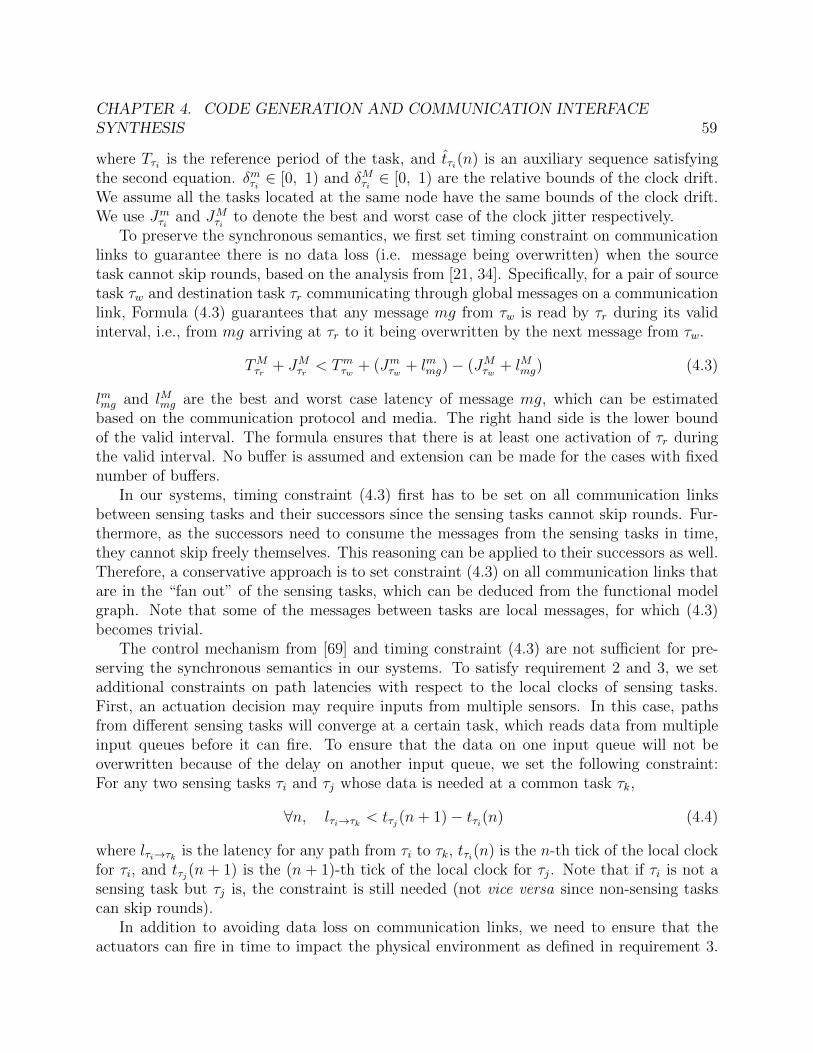
The set of tasks in F is denoted as T = {τ1, τ2, ..., τm}. Each task τi is periodicallyactivated with period Tτi . Strictly speaking, since the architecture we consider is looselytime-triggered, the periodical tasks are following the local clocks that may have drifts andjitters. To reduce the problem complexity, we assume a fixed period for each task in mapping,and leave the consideration of clock drifts and jitters to the code generation step, as shownlater in Chapter 4.
Tasks are scheduled with preemption according to their priorities, and a total order existsamong the task priorities on each node. We use oτi,τj to denote the priority relation betweentask τi and τj, i.e. oτi,τj is 1 if τj has a higher priority than τi, 0 otherwise. Computationalnodes can be heterogeneous, and tasks can have different execution times on different nodes.We use Cτi,pj to denote the worst case execution time of task τi on computation componentpj, which can be obtained via either static analysis or dynamic profiling. Mτi,pj denotes therequired instruction memory for τi on pj. We denote the set of tasks that must be mappedonto processors as T ′, which is a subset of T excluding sensing and actuating tasks (asexplained above, they are one-to-one mapped to manually chosen sensors and actuators).
We use Boolean variable aτi,pj to represent whether task τi is mapped onto computationcomponent pj (1 if mapped, 0 otherwise). Pτi denotes the set of candidate computationcomponents that τi can be mapped to. If τi is a sensing or actuating task, value of aτi,pj isdecided by the manual selection and Pτi is set to the chosen sensor or actuator. Booleanvariable hτi,τj denotes whether τi and τj are mapped onto the same computation component.
CHAPTER 3. MAPPING 25
Boolean variable spj denotes whether processor pj ∈ P ′ is selected.For a signal si, srcsi and {dstsi,j} denote the source task and the set of destination
tasks of signal si, respectively (communication may be of multicast type). The computa-tional nodes to which the source task srcsi and the destination task dstsi,j are allocatedare called source and destination nodes, respectively. If the source node is the same asall the destination nodes, the signal is local. Otherwise, it is global and must be packedinto a message transmitted on the network between the source node and all its destinationnodes. In this mapping problem, we assume each signal si is packed into its own message,denoted by mi (in Section 3.3, we will explore signal packing for CAN-bus based systems).M = {m1,m2, ...,ml} denotes the set of messages communicated between tasks. Similarlyas for signals, srcmi and dstmi denote the source task and destination task of message mi.Boolean variable gmi is 1 if mi is a global message, i.e. srcmi and dstmi are mapped to differ-ent components, otherwise gmi is 0. Variable lmi denotes the worst case transmission delay ofmi, which represents the largest time interval from srcmi sending mi to dstmi receiving mi.The value of lmi depends on which computation components srcmi and dstmi are mappedto, and the communication latency between the components. We use Lpi,pj to denote thecommunication latency from computation component pi to pj, which can be estimated basedon the given physical locations of sensors, actuators and candidate processors. Note that thisis only a high level estimation of the latency without the details of communication network.In the case that pi = pj, Lpi,pj represents the local communication latency between two taskson the same computation component.
3.2.1.1 End-to-End Latency
A path ρ on the application graph G is an ordered interleaving sequence of tasks and signals,defined as ρ = [τr1 , sr1 , τr2 , sr2 , ..., srk−1
, τrk ]. src(ρ) = τr1 is the path’s source task andsnk(ρ) = τrk is its sink task. Source tasks are activated by external events, while sink tasksactivate actuators. A typical path for BAC systems would start from a sensing task, passthrough tasks running control algorithms, and end at an actuating task. Multiple pathsmay exist between each source-sink pair. The worst case end-to-end latency incurred whentraveling a path ρ is denoted as lρ. The path deadline for ρ, denoted by dρ, is an applicationrequirement that may be imposed on selected paths.
Let rτi denote the worst case response time of a task τi, which is the largest time intervalfrom the activation of the task to its completion. Let lsi denote the worst case transmissiontime of a signal si. In this problem, si is mapped to its own message mi, therefore lsi = lmi ,and mi ∈ ρ if and only if si ∈ ρ. The worst case end-to-end latency of a path can becomputed as follows.
lρ =∑τi∈ρ
rτi +∑mi∈ρ
lmi +∑
mi∈ρ∧mi∈GS
Tdstmi (3.1)
where GS is the set of all global messages. The periods of the destination tasks of globalmessages are included in the latency because of the asynchronous nature of the communica-
CHAPTER 3. MAPPING 26
tion. In the worst case, the input global message of a periodical task may arrive immediatelyafter the task was just activated and has to wait for an activation period of the task beforeit can be read. The formula is similar to one in [33, 78], except that here message latenciesare more abstract since we do not have the details of the communication network at thisstage of the design.
3.2.1.2 Task Response Time Analysis
The computation of worst case task response time rτi depends on the scheduling policy of theprocessor to which the task is mapped. In our case study, we assume the processors employa preemptive scheduling based on pre-assigned priorities. Under this assumption and in thecase of rτi ≤ Tτi , rτi can be computed as follows, based on the analysis from [33, 50].
rτi = Cτi +∑
τj∈hp(τi)
⌈rτiTτj
⌉Cτj (3.2)
where hp(τi) refers to the set of higher priority tasks on the same processor.
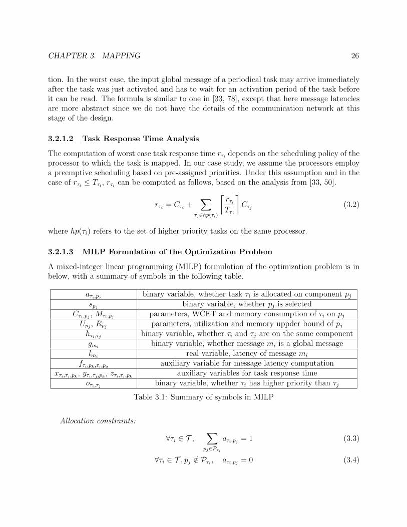
3.2.1.3 MILP Formulation of the Optimization Problem
A mixed-integer linear programming (MILP) formulation of the optimization problem is inbelow, with a summary of symbols in the following table.
aτi,pj binary variable, whether task τi is allocated on component pjspj binary variable, whether pj is selected
Cτi,pj , Mτi,pj parameters, WCET and memory consumption of τi on pjUpj , Rpj parameters, utilization and memory uppder bound of pjhτi,τj binary variable, whether τi and τj are on the same componentgmi binary variable, whether message mi is a global messagelmi real variable, latency of message mi
fτi,pk,τj ,pq auxiliary variable for message latency computationxτi,τj ,pk , yτi,τj ,pk , zτi,τj ,pk auxiliary variables for task response time
oτi,τj binary variable, whether τi has higher priority than τj
Table 3.1: Summary of symbols in MILP
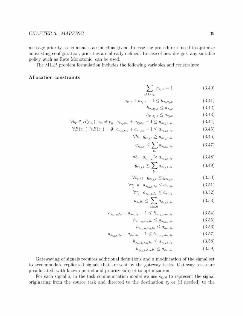
Allocation constraints:
∀τi ∈ T ,∑pj∈Pτi
aτi,pj = 1 (3.3)
∀τi ∈ T , pj /∈ Pτi , aτi,pj = 0 (3.4)
CHAPTER 3. MAPPING 27
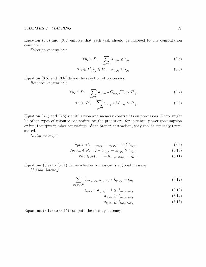
Equation (3.3) and (3.4) enforce that each task should be mapped to one computationcomponent.
Selection constraints:
∀pj ∈ P ′,∑τi∈T ′
aτi,pj ≥ spj (3.5)
∀τi ∈ T ′, pj ∈ P ′, aτi,pj ≤ spj (3.6)
Equation (3.5) and (3.6) define the selection of processors.Resource constraints:
∀pj ∈ P ′,∑τi∈T ′
aτi,pj ∗ Cτi,pj/Tτi ≤ Upj (3.7)
∀pj ∈ P ′,∑τi∈T ′
aτi,pj ∗Mτi,pj ≤ Rpj (3.8)
Equation (3.7) and (3.8) set utilization and memory constraints on processors. There mightbe other types of resource constraints on the processors, for instance, power consumptionor input/output number constraints. With proper abstraction, they can be similarly repre-sented.
Global message:
∀pk ∈ P , aτi,pk + aτj ,pk − 1 ≤ hτi,τj (3.9)
∀pk, pq ∈ P , 2− aτi,pk − aτj ,pq ≥ hτi,τj (3.10)
∀mi ∈M, 1− hsrcmi ,dstmi = gmi (3.11)
Equations (3.9) to (3.11) define whether a message is a global message.Message latency: ∑
pk,pq∈P
fsrcmi ,pk,dstmi ,pq ∗ Lpk,pq = lmi (3.12)
aτi,pk + aτj ,pq − 1 ≤ fτi,pk,τj ,pq (3.13)
aτi,pk ≥ fτi,pk,τj ,pq (3.14)
aτj ,pq ≥ fτi,pk,τj ,pq (3.15)
Equations (3.12) to (3.15) compute the message latency.
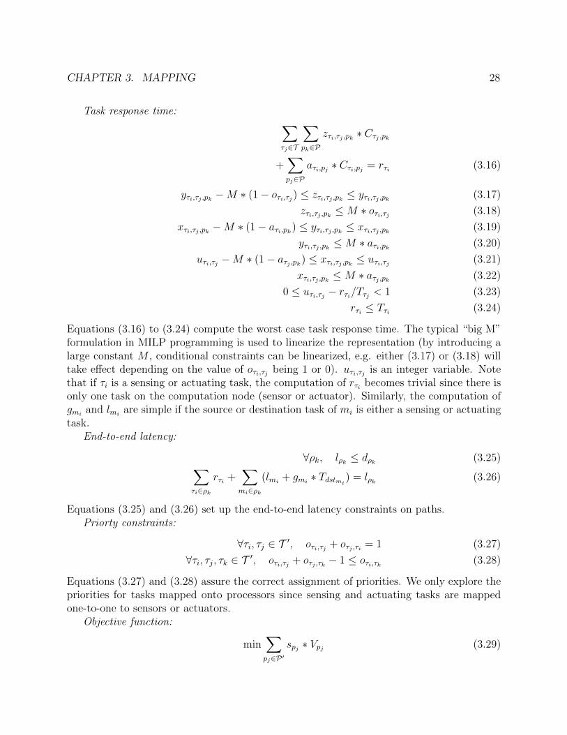
Equations (3.16) to (3.24) compute the worst case task response time. The typical “big M”formulation in MILP programming is used to linearize the representation (by introducing alarge constant M , conditional constraints can be linearized, e.g. either (3.17) or (3.18) willtake effect depending on the value of oτi,τj being 1 or 0). uτi,τj is an integer variable. Notethat if τi is a sensing or actuating task, the computation of rτi becomes trivial since there isonly one task on the computation node (sensor or actuator). Similarly, the computation ofgmi and lmi are simple if the source or destination task of mi is either a sensing or actuatingtask.
End-to-end latency:
∀ρk, lρk ≤ dρk (3.25)∑τi∈ρk
rτi +∑mi∈ρk
(lmi + gmi ∗ Tdstmi ) = lρk (3.26)
Equations (3.25) and (3.26) set up the end-to-end latency constraints on paths.Priorty constraints:
Equations (3.27) and (3.28) assure the correct assignment of priorities. We only explore thepriorities for tasks mapped onto processors since sensing and actuating tasks are mappedone-to-one to sensors or actuators.
Objective function:
min∑pj∈P ′
spj ∗ Vpj (3.29)
CHAPTER 3. MAPPING 29
Finally, Equation (3.29) is the objective function. It does not include the costs of sensors,actuators and communication network. Since we assume sensors and actuators are chosenmanually, their costs are not in the objective function. The communication network willbe optimized later in the mapping flow, and we do not have an accurate way to estimateits cost at this stage yet. In our future work, we plan to extract high level informationof the communication networks and include an abstract model of their cost in the MILPformulation.
By solving the MILP above, we select processors, allocation of tasks and priority assign-ment of tasks. These will be used for constructing a mapped model, which serves as theinput of communication network synthesis.
3.2.2 Communication Network Synthesis
As shown in Figure 3.1, the communication network synthesis step takes a mapped modelGC = (VC , EC) as input, and refines its virtual communication components EC to a specificnetwork of communication links, routers and repeaters.
We use COSI (Communication Synthesis Infrastructure) [57]1 for our communicationnetwork synthesis. The MILP introduced above provides the inputs to COSI. Specifically,the selected computation components and allocated tasks define VC in graph GC . Eachcomputation component is labeled with parameters for representing certain characteristicssuch as cost, physical location, etc. The virtual communication components EC on whichthe messages are allocated can be deduced from the MILP results. For two computationcomponents, if there are tasks on them exchanging global messages, a virtual communicationcomponent is needed to connect them, and those global messages are naturally allocated tothis virtual communication component. The traffic load and latency requirement on eachvirtual communication component can then be deduced.
3.2.3 Case Study
We applied our mapping formulation and algorithm to the room temperature control exampleshown in Figure 2.1. To test the scalability of the algorithm, we extended the number ofrooms from 3 to more than 40, while keeping the same structure. The building floorplanand physical constraints are from a real office building. The functional model consists of 61sensing tasks, 1 LQR task, 61 PID tasks and 61 actuating tasks. There are 61 paths fromsensing task to LQR to PID then to actuating task. The total number of messages is 183.The architecture platform is characterized in Table 3.2, part of which is the same as in [53].We use ARCNET [2] daisy chain buses as communication library.
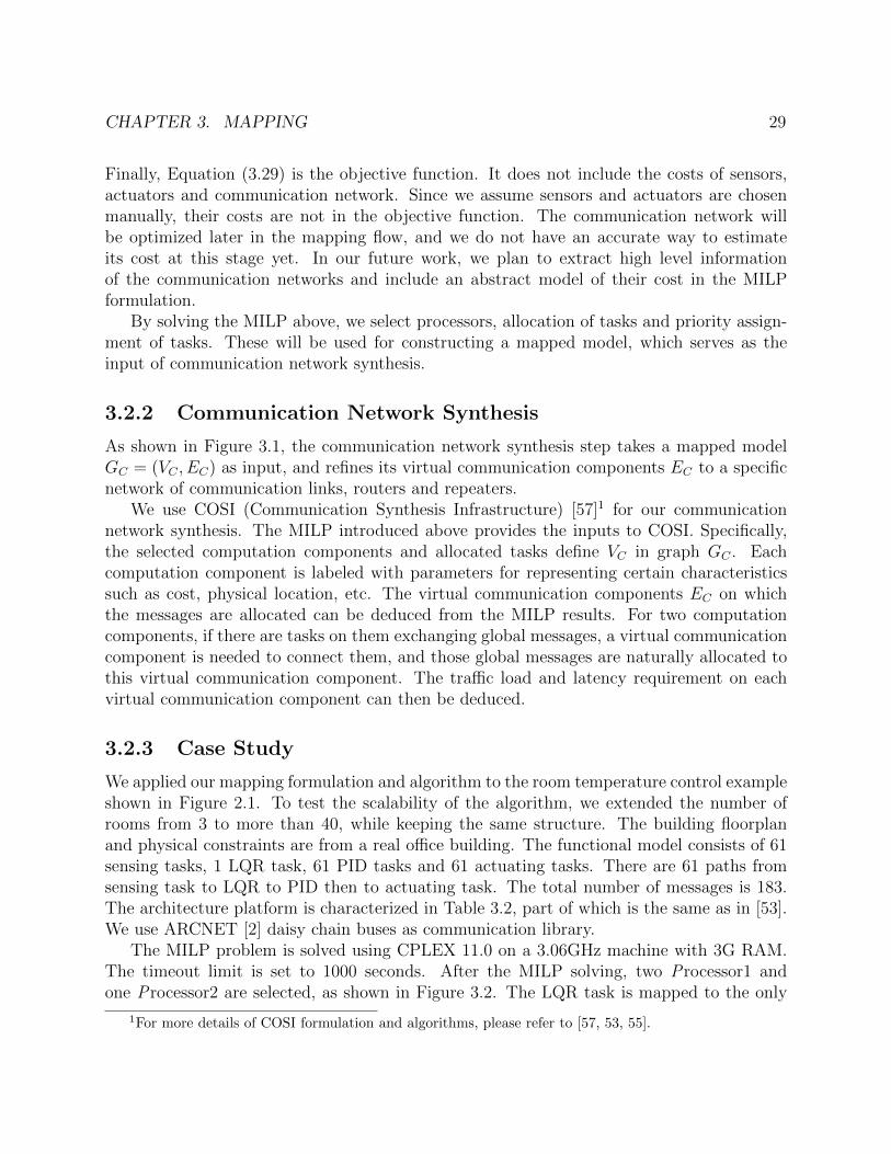
The MILP problem is solved using CPLEX 11.0 on a 3.06GHz machine with 3G RAM.The timeout limit is set to 1000 seconds. After the MILP solving, two Processor1 andone Processor2 are selected, as shown in Figure 3.2. The LQR task is mapped to the only
1For more details of COSI formulation and algorithms, please refer to [57, 53, 55].
CHAPTER 3. MAPPING 30
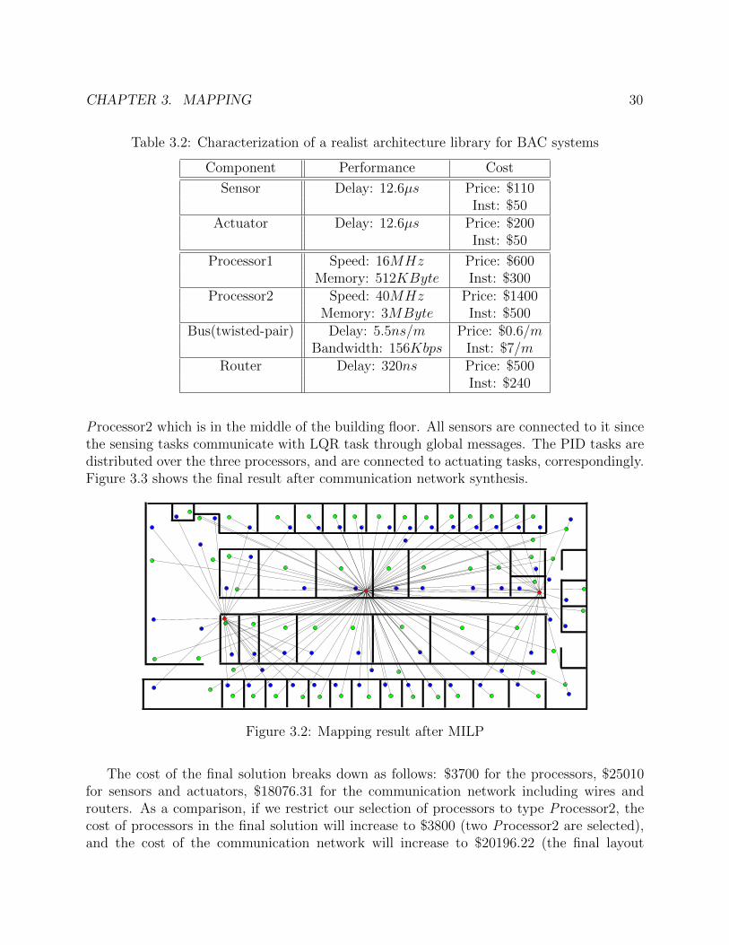
Table 3.2: Characterization of a realist architecture library for BAC systems
Processor2 which is in the middle of the building floor. All sensors are connected to it sincethe sensing tasks communicate with LQR task through global messages. The PID tasks aredistributed over the three processors, and are connected to actuating tasks, correspondingly.Figure 3.3 shows the final result after communication network synthesis.
Figure 3.2: Mapping result after MILP
The cost of the final solution breaks down as follows: $3700 for the processors, $25010for sensors and actuators, $18076.31 for the communication network including wires androuters. As a comparison, if we restrict our selection of processors to type Processor2, thecost of processors in the final solution will increase to $3800 (two Processor2 are selected),and the cost of the communication network will increase to $20196.22 (the final layout
CHAPTER 3. MAPPING 31
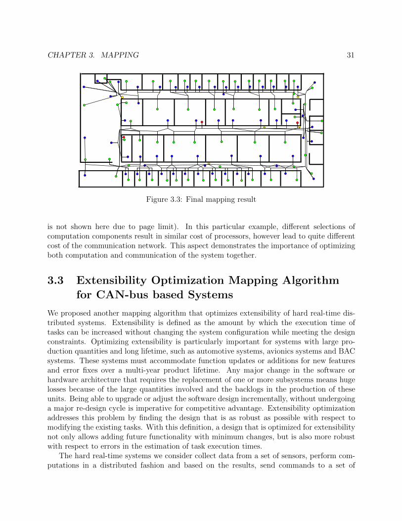
Figure 3.3: Final mapping result
is not shown here due to page limit). In this particular example, different selections ofcomputation components result in similar cost of processors, however lead to quite differentcost of the communication network. This aspect demonstrates the importance of optimizingboth computation and communication of the system together.
3.3 Extensibility Optimization Mapping Algorithm
for CAN-bus based Systems
We proposed another mapping algorithm that optimizes extensibility of hard real-time dis-tributed systems. Extensibility is defined as the amount by which the execution time oftasks can be increased without changing the system configuration while meeting the designconstraints. Optimizing extensibility is particularly important for systems with large pro-duction quantities and long lifetime, such as automotive systems, avionics systems and BACsystems. These systems must accommodate function updates or additions for new featuresand error fixes over a multi-year product lifetime. Any major change in the software orhardware architecture that requires the replacement of one or more subsystems means hugelosses because of the large quantities involved and the backlogs in the production of theseunits. Being able to upgrade or adjust the software design incrementally, without undergoinga major re-design cycle is imperative for competitive advantage. Extensibility optimizationaddresses this problem by finding the design that is as robust as possible with respect tomodifying the existing tasks. With this definition, a design that is optimized for extensibilitynot only allows adding future functionality with minimum changes, but is also more robustwith respect to errors in the estimation of task execution times.
The hard real-time systems we consider collect data from a set of sensors, perform com-putations in a distributed fashion and based on the results, send commands to a set of
CHAPTER 3. MAPPING 32
actuators. We focus on systems that are based on priority-based scheduling of periodic tasksand messages. Each input data (generated by a sensor, for instance) is available at one of thesystem’s computational nodes. A periodically activated task on this node reads the inputdata, computes intermediate results, and writes them to the output buffer from where theycan be read by another task or used for assembling the data content of a message. Messages- also periodically activated - transmit the data from the output buffer on the current nodeover the bus to an input buffer on a remote node. Local clocks on different nodes are notsynchronized. Tasks may have multiple fan-ins and messages can be multi-cast. Eventually,task outputs are sent to the system’s output devices or actuators.
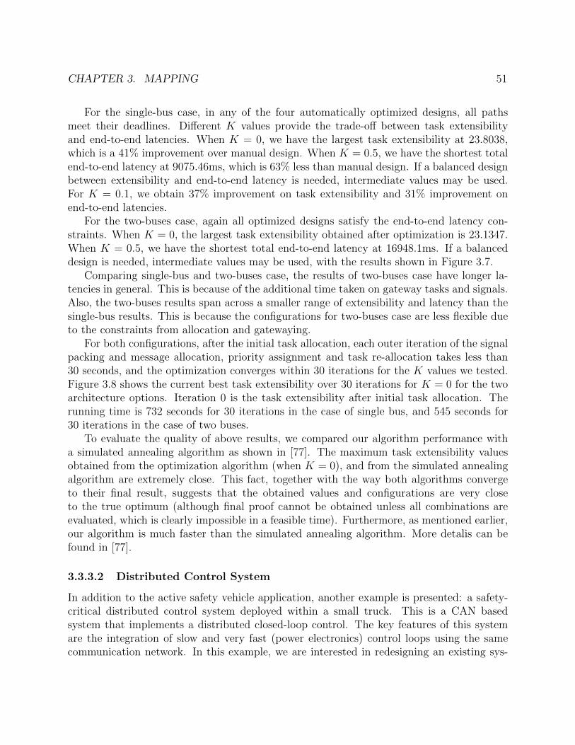
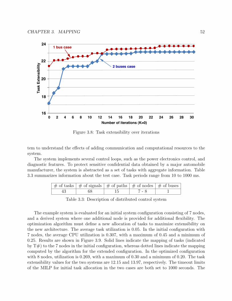
The architecture platform is given in this case, which consists of a set of ECUs connectedby CAN buses. The design space includes task allocation and priority assignment, signalpacking and message priority assignment. Following the idea of the general mapping flowdiscussed in Section 3.1, we designed a two-stage algorithm for the mapping problem. Thefirst stage of the algorithm is based on mixed integer linear programming (MILP), wheretask allocation (the most important variable with respect to extensibility) is optimized withindeadline and utilization constraints. The second stage features three heuristic steps, whichiteratively pack signals to messages, assign priorities to tasks and messages, and explore taskre-allocation. This algorithm runs much faster than randomized optimization approaches (a20x reduction with respect to simulated annealing as shown in [77]). Hence, it is applicable toindustrial-size systems as shown by the experimental case studies in Section 3.3.3, addressingthe typical case of the deployment of additional functionalities in a commercial car. Theshorter running time of the proposed algorithm allows using the method not only for theoptimization of a given system configuration, but also for architecture exploration, where thenumber of system configurations to be evaluated and subject to optimization can be large.
A further advantage of an MILP formulation (even if used only for the first stage) withrespect to randomized optimization, is the possibility of leveraging mature technology insolvers, the capability of detecting the actual optimum (when found in reasonable time), or,when the running time is excessive, to compute at any time a lower bound on the cost ofthe optimum solution, which allows to evaluate the quality of the best solution obtained upto that point.
3.3.1 Representation
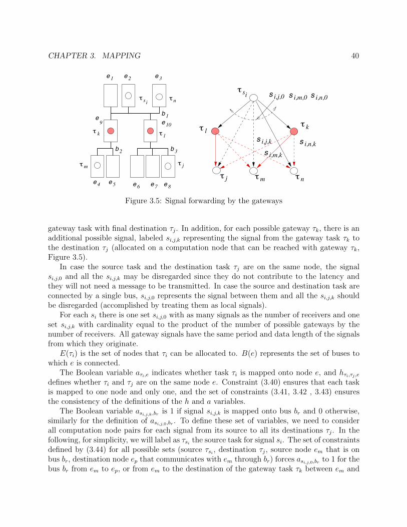
The problem representation has some similarities with the mapping problem introduced inSection 3.2, but also has its uniqueness due to the consideration of gateways, signal packingand most importantly the extensibility metric.
The application is represented as a directed graph G = (T ,S) as discussed in Section 3.1.The application is mapped onto an architecture that consists of a set of computational nodes,denoted as E = {e1, e2, ..., ep}, connected through a set of CAN buses B = {b1, b2, ..., bq}.
τi is periodically activated with period tτi , and executed with priority pτi . The periods ofcommunicating tasks are assumed to be harmonic, which is almost always true in practicaldesigns. Tasks are scheduled with preemption according to their priorities, and a total order
CHAPTER 3. MAPPING 33
exists among the task priorities on the same node. Tasks can have different execution timeson different nodes. We use cτi,e to denote the execution time of task τi on node e. In thefollowing, the e subscript is dropped whenever the formula refers to tasks on a given node,and e is implicitly defined, or when the task allocation is (at least temporarily) defined, andthe node to which the computation time (or its extensibility ∆c) refers, is known. Finally,rτi denotes the worst case response time.
A global signal si, whose source node is different than the destination node, must bepacked into a message transmitted on the buses between the source node and all its destina-tion nodes. Only signals with the same period, same source node and same communicationbus can be packed into the same message. For message mi, tmi denotes its period, pmi denotesits priority, and cmi denotes its worst case transmission time on a bus with unit speed. Theworst transmission time on bus bj is cmi/speedbj , where speedbj is the transmission speed ofbj. rmi is the worst case response time on a bus with unit speed.
In addition, in complex systems the source and destination tasks may not reside oncomputation nodes that share the same bus. In this case, a signal exchanged among themwill have to go through a gateway node and be forwarded by a gateway task. We includethe gateway concept in our model with a number of restrictive (but hopefully realistic)assumptions.
• any communication between two computation nodes is never going to need more thanone gateway hop (every bus is connected to all the others through one gateway compu-tation node). This assumption, realistic for small systems, could probably be removedat the price of additional complexity.
• a single gateway node connects any two buses.
• a single task is responsible for signal forwarding on each gateway node. This task isfully determined (there might be other tasks running on the gateway node.)
A path p on the application graph G is an ordered interleaving sequence of tasks andsignals, defined as p = [τr1 , sr1 , τr2 , sr2 , ..., srk−1
, τrk ], where src(p) = τr1 is the path’s sourceand snk(p) = τrk is its sink. Multiple paths may exist between each source-sink pair. Theworst case end-to-end latency of path p is denoted as lp, and the path deadline of p is denotedby dp.
It may be argued that today, it is industrial practice (at least in the automotive domain)to allocate resources between suppliers before implementation parameters (such as worst-case execution times) are known. This is however only partly true. A major architectureand functional redesign is often characterized by a significant reuse (or carry-over) of pre-existing functionality (60% to 70% are typical figures), for which these estimates could beavailable. In addition, rapid prototyping techniques and the increased use of automatic codegeneration tools should ease the availability of these implementation related parameters (orat least estimates) even for newly-designed functions.
CHAPTER 3. MAPPING 34
3.3.1.1 Design Space and Extensibility Metric
The design problem can be defined as follows. Given a set of design constraints including:• end-to-end deadlines on selected paths• utilization bounds on nodes and buses• maximum message sizes
explore the design space that includes:• allocation of tasks to computational nodes• packing of signals and allocation of messages to buses• assignment of priorities to tasks and messages
to maximize task extensibility.Different definitions can be provided for task extensibility. The main definition used in
this work is as the weighted sum of each task’s execution time slack over its period:
max. S =∑τi∈T
wτi∆cτitτi
(3.30)
where a task’s execution time slack ∆cτi is defined as the maximum possible increase of itsexecution time cτi without violating the design constraints, assuming the execution times ofother tasks are not changed.
wτi is a preassigned weight that indicates how likely and how much the task’s executiontime will be increased in future functionality extensions. In practice, however, because offunctional dependencies, execution time increases in tasks belonging to a set might needto be considered jointly. This can be done in several ways. One possible way is in theassignment of the wτi weights as follows.
1. Identify a set of update scenarios u1, u2, ...un. Each scenario uk includes a group oftasks Tk to be extended, and is assigned a likelihood probability pk.
2. For each update scenario uk and τi ∈ Tk, assign a weight wik to represent how muchthe task’s execution time will be increased in this scenario.
3. The final weight wτi of a task is computed as wτi =∑
k:τi∈Tk pk ∗ wik .
A more explicit way is to identify groups of tasks that are functionally related so that theirexecution times increases are related (in a way expressed by a simple linear formulation).
We identify a set of task groups TG = {Tg1 , Tg2 , ...Tgn} (each gi ∈ G representing anupdate scenario). Execution times of tasks belonging to the same group are bound toincrease together in each update scenario. For each task τj ∈ Tgi , we model the possibleadditional execution time as
∆cτj ,gi = Aτj ,gi ∗∆cgi (3.31)
CHAPTER 3. MAPPING 35
where Aτj ,gi is a constant. Equation (3.31) represents a simple extensibility dependencyamong tasks belonging to a functional group (more complex relationships can be representedat the price of higher complexity.)
Based on Equation (3.31), we define this alternative extensibility metric as follows.
max. S =∑gi∈G
wgi ∗∆cgi (3.32)
Finally, another formulation is to use execution time slack over original execution time,i.e. ∆cτi/cτi , instead of using execution time slack over period in Equation (3.30).
The metric function (3.30) is used in the following discussion of the optimization algo-rithm. The required changes for the adoption of the metric in (3.32) are discussed furtherin Section 3.3.2.6. The comparison of the metric function (3.30) with the metric that usesslack times relative to the original execution time can be found in [77].
3.3.1.2 End-to-End Latency
After tasks are allocated, some signals are local, and their transmission time is assumed tobe zero. Others are global, and need to be transmitted on the buses through messages. Thetime needed to transmit a global signal is equal to the transmission time of the correspondingmessage. Let rsi denote the worst case response time of a global signal si, and assume itscorresponding message is mj, then rsi = rmj .
The worst case end-to-end latency can be computed for each path by adding the worstcase response times of all the tasks and global signals on the path, as well as the periods ofall the global signals and their destination tasks on the path.
lp =∑τi∈p
rτi +∑
si∈p∧si∈GS
(rsi + tsi + tdstsi ) (3.33)
where GS is the set of all global signals. Of course, in the case that gateways are used acrossbuses, the signals to and from possible gateway tasks, as well as the response time of thegateway task itself and the associated sampling delays must be included in the analysis.
We need to include periods of global signals and their destination tasks because of theasynchronous sampling of communication data. In the worst case, the input global signalarrives immediately after the completion of the first instance of task τi. The event data willbe read by the task on its next instance and the result will be produced after its worst caseresponse time, that is, tτi + rτi time units after the arrival of the input signal. The samereasoning applies to the execution of all tasks that are the destinations of global signals,and applies to global signals themselves. However, for local signals, the destination task canbe activated with a phase (offset) equal to the worst-case response time of the source task,under our assumption that their periods are harmonic. In this case, we only need to add the
CHAPTER 3. MAPPING 36
response time of the destination task. When a task has more than one local predecessor ona time-critical path, its activation phase (offset) will have to be set to the largest among thecompletion times of its predecessors. This case could be dealt with in the previous Equation(3.33) and in the following formulations, by replacing the response time contribution of localsender tasks with the maximum among the response times of all the senders for a given taskin the path. Similarly, it is sometimes possible to synchronize the queuing of a message fortransmission with the execution of the source tasks of the signals present in that message.This would reduce the worst case sampling period for the message transmission and decreasethe latency in Equation (3.33). In this work, we do not consider these possible optimizationsand leave them to future extensions.
Task Response TimesThe analysis and calculation of task response times is the same as in the previous mapping
problem for BAC systems (Equation (3.2)).
rτi = Cτi +∑
τj∈hp(τi)
⌈rτiTτj
⌉Cτj (3.34)
Message Response TimesWorst case message response times are calculated similarly to task response times. The
main difference is that message transmissions on the CAN bus are not preemptable. There-fore, a message mi may have to wait for a blocking time Bmax, which is the longest transmis-sion time of any frame in the system. Likewise, the message itself is not subject to preemptionfrom higher priority messages during its own transmission time cmi . The response time cantherefore be calculated with the following recurrence relation, in the case of rmi ≤ tmi :
rmi = cmi +Bmax +∑
mj∈hp(mi)
⌈rmi − cmi
tmj
⌉cmj (3.35)
3.3.1.3 Formulation
Based on the formulas for computing end-to-end latencies and response times, we constructa mathematical formulation that contains all the design variables. Part of the formulation issimilar to the one in [76]: both explore the same set of design variables - task allocation, signalpacking and message allocation, as well as task and message priorities. In [76], the problemwas formulated as mixed integer linear programming (MILP). To reduce the complexity, theproblem was divided into sub-problems and solved by a two-step approach.
However, in [76], the objective is to minimize end-to-end latencies, while in this work,we optimize task extensibility. The formulation of task extensibility with respect to end-to-end deadline constraints is a quite challenging task. In general, inverting the function
CHAPTER 3. MAPPING 37
that computes response times as a function of the task execution times is of exponentialcomplexity in the simple case of single-CPU scheduling [22]. When dealing with end-to-endconstraints, the problem is definitely more complex. A possible approach consists of a verysimple (but possibly time-expensive) bisection algorithm that finds the sensitivity of end-to-end response times with respect to increases in task execution times (this is the solutionused for performing sensitivity analysis in [62]).
Formally, if ∆rij denotes the increase of task τj’s response time rτj when task τi’s com-putation time cτi is increased by ∆cτi , the end-to-end latency constraints and utilizationconstraints are expressed as follows:∑
τj∈p∧τj∈(lp(τi)∪{τi})
∆rij ≤ dp − lp ∀p, ∀τi ∈ T (3.36)
∆cτitτi
+∑
τj∈T (e)
(cτjtτj
) ≤ ue ∀e, ∀τi ∈ T (e) (3.37)
where lp(τi) refers to the set of tasks with priority lower than pτi and executed on the samenode as τi, T (e) denotes the set of the tasks on computational node e, and ue denotes themaximum utilization allowed on e.
The relation between ∆rij and ∆cτi can be derived from Equation (3.2), as follows.
∆rij =∑
τk∈hp(τj)
(
⌈rτj + ∆rij
tτk
⌉−⌈rτjtτk
⌉)cτk
+
⌈rτj + ∆rij
tτi
⌉∆cτi ∀τj ∈ lp(τi) (3.38)
∆rii = ∆cτi +∑
τk∈hp(τi)
(
⌈rτi + ∆rii
tτk
⌉−⌈rτitτk
⌉)cτk (3.39)
For brevity, above formulas do not model task allocation and priority assignment asvariables. In the complete formulation, they were expanded to include those variables.
Contrary to the problem in [76], in our case the formulation cannot be linearized becauseof the second term in Equation (3.38). It could be solved by nonlinear solvers but thecomplexity is in general too high for industrial size applications. Therefore, we propose analgorithm that defines two stages to decompose the complexity: one in which mathematicalprogramming (MILP) is used, and one refinement stage that consists of several steps basedon heuristics.
3.3.2 Optimization Algorithm
The flow of our algorithm is shown in Figure 3.4. First, we decide the allocation of tasks,since the choices of other design variables are restricted by task allocation. In the initialallocation stage, the problem is formulated as MILP and solved by an MILP solver. Then
CHAPTER 3. MAPPING 38
Initial Task Allocation (MILP in Section 3.3.2.1)
Signal Packing and Message Allocation
(Section 3.3.2.2)
Task and Message Priority Assignment
(Section 3.3.2.3)
Task Re-allocation (Algorithm 2 in Section 3.3.2.4)
Reach Stop Condition?
Yes
End
No
Figure 3.4: Algorithm flow for task extensibility optimization
a series of heuristics is used in the refinement stage: in the signal packing and messageallocation step, a heuristic is used to decide signal-to-message packing and message-to-busallocation. In the task and message priority assignment step, an iterative method is designedto assign the priorities of tasks and messages. After these steps are completed, if the designconstraints cannot be satisfied or if we want to further improve extensibility, the tasks can bere-allocated and the process repeated. Because of the complexity of the MILP formulation,we designed a heuristic for task re-allocation, based on the extensibility and end-to-endlatency values obtained in the previous steps.
3.3.2.1 Initial Task Allocation
In the initial task allocation stage, tasks are mapped onto nodes while meeting the utilizationand end-to-end latency constraints. Utilization constraints are considered in place of the trueextensibility metric to allow a linear formulation. In this stage, we also allocate signals tomessages and buses assuming each message contains one signal only. The initial tasks and
CHAPTER 3. MAPPING 39
message priority assignment is assumed as given. In case the procedure is used to optimizean existing configuration, priorities are already defined. In case of new designs, any suitablepolicy, such as Rate Monotonic, can be used.
The MILP problem formulation includes the following variables and constraints:
Allocation constraints ∑e∈E(τi)
aτi,e = 1 (3.40)
aτi,e + aτj ,e − 1 ≤ hτi,τj ,e (3.41)
hτi,τj ,e ≤ aτi,e (3.42)
hτi,τj ,e ≤ aτj ,e (3.43)
∀br ∈ B(em), em 6= ep aτsi ,em + aτj ,ep − 1 ≤ asi,j,0,br (3.44)
Gatewaying of signals requires additional definitions and a modification of the signal setto accommodate replicated signals that are sent by the gateway tasks. Gateway tasks arepreallocated, with known period and priority subject to optimization.
For each signal si in the task communication model we use si,j,0 to represent the signaloriginating from the source task and directed to the destination τj or (if needed) to the
CHAPTER 3. MAPPING 40
i
i,n,ks i,m,k
s i,j,k
s i,j,0 s i,n,0s i,m,0! si
!
! n!
!
s
m j
b b
b 1
2 3
k!
e 1 e 2 e 3
e 4 e 5 e 6 e 7 e 8
e9 e 10
! l
! ! !m
! kl!
j n
s
Figure 3.5: Signal forwarding by the gateways
gateway task with final destination τj. In addition, for each possible gateway τk, there is anadditional possible signal, labeled si,j,k representing the signal from the gateway task τk tothe destination τj (allocated on a computation node that can be reached with gateway τk,Figure 3.5).
In case the source task and the destination task τj are on the same node, the signalsi,j,0 and all the si,j,k may be disregarded since they do not contribute to the latency andthey will not need a message to be transmitted. In case the source and destination task areconnected by a single bus, si,j,0 represents the signal between them and all the si,j,k shouldbe disregarded (accomplished by treating them as local signals).
For each si there is one set si,j,0 with as many signals as the number of receivers and oneset si,j,k with cardinality equal to the product of the number of possible gateways by thenumber of receivers. All gateway signals have the same period and data length of the signalsfrom which they originate.
E(τi) is the set of nodes that τi can be allocated to. B(e) represents the set of buses towhich e is connected.
The Boolean variable aτi,e indicates whether task τi is mapped onto node e, and hτi,τj ,edefines whether τi and τj are on the same node e. Constraint (3.40) ensures that each taskis mapped to one node and only one, and the set of constraints (3.41, 3.42 , 3.43) ensuresthe consistency of the definitions of the h and a variables.
The Boolean variable asi,j,k,br is 1 if signal si,j,k is mapped onto bus br and 0 otherwise,similarly for the definition of asi,j,0,br . To define these set of variables, we need to considerall computation node pairs for each signal from its source to all its destinations τj. In thefollowing, for simplicity, we will label as τsi the source task for signal si. The set of constraintsdefined by (3.44) for all possible sets (source τsi , destination τj, source node em that is onbus br, destination node ep that communicates with em through br) forces asi,j,0,br to 1 for thebus br from em to ep, or from em to the destination of the gateway task τk between em and
CHAPTER 3. MAPPING 41
ep. The following set (3.45) sets asi,j,k,br to 1 (if necessary) for the bus br from the gatewayto the destination node ep when gatewaying is needed (in this set of constraints, ep is onbr while em is not). The variables asi,j,k,br have a positive contribution to the cost function,hence they will be set to 0 by the optimization engine, unless forced at 1 by the constraints.
To give an example of these constraints, in Figure 3.5 the condition for the outgoingsignal si,j,0 from τsi to τj to be on bus b1, expressed as
aτsi ,em + aτj ,ep − 1 ≤ asi,j,0,b1
needs to be defined for each computation node pair (m, p) where m ∈ {1, 2, 3} and p 6= m,or m ∈ {9} and p ∈ {1, 2, 3, 10}, or m ∈ {10} and p ∈ {1, 2, 3, 9}. Similar sets of conditionswill then need to be defined for b2 and b3.
As an example of gatewaying, the condition for the mapping on b2 of the (possible) signalforwarded by gateway τk as part of the communication from τsi to τj in the figure is expressedby the set.
aτsi ,em + aτj ,ep − 1 ≤ asi,j,m,b2
defined for all the computation node pairs (m, p) where m ∈ {1, 2, 3, 10} and p ∈ {4, 5}.The value of the Boolean variable gsi,j,0 is 1 if si,j,0 is a global signal (i.e., being transferred
on bus), and 0 otherwise. Similarly, gsi,j,k is 1 if the signal si,j,k (si forwarded by gatewayτk) is global. The definition of gsi,j,0 and gsi,j,k is provided by constraints (3.46-3.47) and(3.48-3.49), respectively. Finally, gsi,j,0 must be 1 if at least one gsi,j,k is 1, as in constraint(3.50).
The Boolean variable asi,br is 1 if signal si needs to be transmitted on bus br (needs amessage on br) and 0 otherwise. constraints (3.51-3.53) encode these conditions.
The Boolean variables hsi,j,0,sm,br and hsi,j,k,sm,brdefine whether si,j,0 and si,j,k share thesame bus br with sm, respectively. Constraints (3.54-3.59) enforce consistency in the defini-tion of the hsi,j,0,sm,br and hsi,j,k,sm,br with respect to the signal-to-bus allocation variables.
Utilization constraints
zτi,e +∑τj∈T
aτj ,e ∗ cτj ,e/tτj ≤ ue (3.60)
∆cτi/tτi −M ∗ (1− aτi,e) ≤ zτi,e (3.61)
zτi,e ≤ ∆cτi/tτi (3.62)
zτi,e ≤M ∗ aτi,e (3.63)∑si∈S
asi,b ∗ csi/tsi/speedb ≤ ub (3.64)
The above constraints enforce the utilization bounds on all nodes and buses consideringthe load of the current tasks (summation on the left-hand side of Equation (3.60) and the
CHAPTER 3. MAPPING 42
additional load caused by extensions of the execution times (zτi,e, on the left-hand side ofthe equation). ue and ub are the utilization bounds on computational node e and bus b,respectively. The additional load caused by the extension ∆cτi must be considered only ifthe task is allocated to the node for which the bound is computed. This is representedby using an additional variable zτi,e, and the typical “big M” formulation in use in MILPprogramming for conditional constraints, where M is a large constant.
In our formulation, tasks can have different execution times depending on their allocation,and cτi,e denotes the worst-case execution time of task τi on node e. Also, buses can havedifferent speeds. csi denotes the transmission time of the message that carries signal si ona bus with unit speed. At this stage, we assume each message will only contain one signal.The transmission time of that message on a bus with speed speedb is csi/speedb.
Latency constraints are derived from Equations (3.33), (3.2) and (3.35). Equation (3.33)shows the calculation of end-to-end latency for path p. For each signal si on path p, we knowits destination task and denote it as τj. If two tasks are on computation nodes connectedto different buses, they will communicate through a gateway task and the correspondingadditional latencies need to be considered. The calculation of end-to-end latency is shownin constraint (3.66). We assume the response time for gateway task τk is cτk (i.e. a gatewaytask has the highest priority on its node).
rτi is the response time of task τi, defined by constraints (3.67-3.72), xτi,τj represents thenumber of possible interference from τj to τi and pτi,τj is a parameter that denotes whethertask τj has higher priority than task τj. A large constant M is used to linearize the relationyτi,τj ,e = xτi,τj ∗ hτi,τj ,e, which defines the number y of actual interferences by higher prioritytasks, similarly as in the utilization constraints. Constraint (3.72) is used to enforce thetask’s response time is no larger than its period, which is the assumption for our responsetime calculation in Equation (3.2).
rsi,j,0 and rsi,j,k represent the response times of the messages that carry signals si,j,0 andsi,j,k, respectively. Their definitions are in constraints (3.73-3.84). If signals are local, thecorresponding response times will be 0. psi,sj , ysi,j,0,sj ,b and ysi,j,k,sj ,b are similarly defined asin the definition of task response time. Constraints (3.78) and (3.84) enforce the assumptionthat message response times should not exceed their periods.
Objective function
max.∑τi∈T
wτi ∗∆cτi/tτi (3.85)
We recall here the objective function in (3.30), which represents the task extensibility.An alternative objective function can also include the optimization of latency, as shown in(3.86). K is the parameter used to explore the trade-off between task extensibility andlatencies. The special case K = 0 is the original objective function (3.85).
CHAPTER 3. MAPPING 44
max.∑τi∈T
wτi ∗∆cτi/tτi −K ∗∑p∈P
lp/dp (3.86)
In Section 3.3.3, we will report the experimental results with various values of K, to showthe relationship between task extensibility and path latencies.
An alternative to the MILP optimization for initial task allocation is to use heuristics.We designed a greedy heuristic algorithm as shown in [77] and compared it with the MILPoptimization. Although the heuristic algorithm is more efficient, the results are much worse.Of course, in principle it is possible to design a better heuristic, but this task is expected to bequite difficult considering the need to balance trade-offs between feasibility and extensibilityand the need to cope with gatewaying (for which the MILP formulation provides intuitivesolutions). For more details, please refer to [77].
3.3.2.2 Signal Packing and Message Allocation
After the allocation of tasks is chosen, we use a simple heuristic to determine the signalpacking and message allocation. The steps are shown below.
1. Group the signals with the same source node and period as packing candidates.
2. Within each group, order the signals based on their priorities, then pack them ac-cording to the message size constraints (priorities are assumed given from an existingconfiguration or some suitable policy, as in the initial task allocation). The priority ofa message is set to the highest priority of the signals that are mapped into it.
3. Assign a weight wmi to each message mi based on its priority, transmission time andperiod. In our algorithm, we set wmi = k1/pmi + k2 ∗ cmi/tmi , where pmi , cmi andtmi are priority, transmission time on bus with unit speed and period of the message.k1 and k2 are constants, whose values are tuned in case studies (both set to 1 in ourexperiments). When multiple buses are available between the source and destinationnodes, we allocate messages to buses according to their weights. Messages with largerweights are assigned first to faster buses.
Other more sophisticated heuristics or mathematical programming solutions have beenconsidered. For instance, signal packing can be formulated as MILP as in [76]. However,from preliminary experiments, there is no significant improvement that can outweigh thespeed of this simple strategy.
3.3.2.3 Priority Assignment
In this step, we assign priorities to tasks and messages, given the task allocation, signalpacking and message allocation obtained from previous steps.
CHAPTER 3. MAPPING 45
This priority assignment problem is proven to be NP-complete [25]. Finding an optimalsolution is generally not feasible for industrial-sized problems. Therefore, we propose aniterative heuristic to solve the problem.
The flow of this heuristic is shown in Figure 3.6. The basic idea is to define the localdeadlines of tasks and messages over iteration steps, then assign priorities based on thedeadlines. Intuitively, shorter deadlines require higher priorities and longer local deadlinescan afford lower priorities.
Initialize Local Deadlines
Reach Stop Condition?
Finish Priority Assignment
Assign Priorities (deadline-monotonic)
Update Local Deadlines
Yes
No
Calculate criticality of every task and message
Update local deadline of every task and message based on its criticality
Initially, the deadlines of tasks and messages are the same as their periods. Then, dead-lines are modified, and priorities are assigned using the deadline-monotonic (DM) approach[12]. Of course, there is no guarantee that the DM policy is optimal in this case as for anysystem with non-preemptable resources (the CAN bus), but there is no optimal counterpartthat can be used here, and DM is a sensible choice in the context of our heuristics.
During the iterations, deadlines are changed based on task and message criticality, asshown in Algorithm 1 and explained below.
The criticality of a task or message, reflects how much the response times along the pathsto which it belongs are affected by extensions in the execution times of other tasks. Tasksand messages with higher criticality are assigned higher priorities. To define the criticalityε of a task or a message, we increase the execution time of each task τi, by UB(∆cτi), themaximum amount allowed by utilization constraints and an upper bound of task executiontime slack, as shown in line 3 and 4 in Algorithm 1. Then, the response time of τi and of
CHAPTER 3. MAPPING 46
Algorithm 1 Update Local Deadline (K1)1: Initialize the criticality ε of every task and message to 02: for all task τi do3: UB(∆cτi) = tτi ∗ (ue −
∑τj∈T (e) cτj/tτj )
4: cτi = cτi + UB(∆cτi)5: for all task τj ∈ (lp(τi) ∪ {τi}) do6: update rτj7: for all path p whose latency is changed do8: if lp > dp then9: for all tasks and messages oj on p do
10: εoj = εoj + wτi ∗ (lp − dp)/toj11: reset all cτi , rτi , lp to the values before the iteration12: for all task τi do13: εNτi = ετi/maxτi∈T {ετi}14: dτi = dτi ∗ (1−K1 ∗ εNτi )15: for all message mi do16: εNmi = εmi/maxmi∈M{εmi}17: dmi = dmi ∗ (1−K1 ∗ εNmi)
lower priority tasks on the same node as τi is recomputed (line 5 and 6). The criticality of theaffected task τj or message mj (both generically denoted as object oj) is defined by addingup a term wτi ∗ (lp − dp)/toj for each path p whose end-to-end latency exceeds the deadlineafter the increase UB(∆cτi), where wτi is the weight of τi (line 7 to 10). After repeating thisoperation for every task, the criticality of all tasks and messages is computed, denoted byεoj . Criticality values are normalized, obtaining a value εN for each task and message andfinally, local deadlines are computed as d = d ∗ (1−K1 ∗ εN) (line 11 to 16). The procedureis shown in Algorithm 1. The parameter K1 is initially set to 1, then adjusted in the lateriteration steps using a strategy that takes into account the number of iteration steps, thenumber of times the current best solution is found, and the number of times the priorityassignment remains unchanged.
As shown in Figure 3.6, after local deadlines are updated, the stop condition for priorityassignment is checked. If the number of iterations reaches its limit, or the upper bound oftask extensibility is reached, the priority assignment will finish, otherwise we keep iterating.
The strategy of changing priorities based on local deadlines can also be found in [35].Different from our algorithm, the goal is only to meet end-to-end latency constraints, there-fore deadlines are updated based on the slack time of tasks or messages which indicate howmuch the local deadlines can be increased without violating latency constraints.
3.3.2.4 Task Re-allocation
As shown in Figure 3.4, after all the design variables are decided, we calculate the value of theobjective function in Formula 3.30, and check the stop condition for our entire algorithm. If
CHAPTER 3. MAPPING 47
the results are not good enough and the iteration limit has not been exceeded, we re-allocatethe tasks and repeat the signal packing, message allocation and priority assignment.
We could use the same MILP based method for re-allocating tasks, with additionalconstraints to exclude the allocations that have been considered. However, solving the MILPis time consuming. To speed up the algorithm, we designed a local optimization heuristicthat leverages the results of previous iterations for the task re-allocation step in Figure 3.4.The details of this heuristic are shown in Algorithm 2.
Algorithm 2 Task Re-allocation (K2)
Let Φ(M) =∑
τi∈T wτi ∗UB(∆cτi)/tτi −K2 ∗∑
p∈P lp/dp for a mapping M
1: if current solution does not satisfy latency constraints then2: K2+ = KC
3: ∆best = MIN4: for all task τi and node e that τi is not on e do5: ∆τi,e = Φ(M ′) − Φ(M) {where M is the original mapping, M ′ is the new mapping after
moving τi to e}6: if ∆τi,e > ∆best then7: best move = τi moves to e8: ∆best = ∆τi,e
9: for all task τi, τj that are not on the same node do10: ∆τi,τj = Φ(M ′)− Φ(M) {M , M ′ similarly defined as above}11: if ∆τi,τj > ∆best then12: best move = switch τi and τj13: ∆best = ∆τi,τj
14: Execute best move
Two operators are considered for generating new configurations: moving one task to adifferent node, or switching two tasks on different nodes. For each possible application ofthe operators on each task or task pair, that satisfies the utilization constraints, we computethe corresponding change of the performance function Φ of Equation (3.86), which includesthe consideration of task extensibility and end-to-end latencies. In the case of multiplebuses, the changes might lead to signal forwarding through gateway tasks, and this is takeninto account in the calculation. Finally the change that provides the largest increase of theperformance function is selected.
Parameter K2 in cost function Φ provides the trade-off between task extensibility andend-to-end latencies. Initially, it is set to the same value as parameter K in Equation (3.86),which is used in the initial task allocation. If the current solution does not satisfy the end-to-end deadlines, we increase K2 by a constant KC to emphasize the optimization of latencies(KC was tuned to 0.05 in our experiments).
CHAPTER 3. MAPPING 48
3.3.2.5 Algorithm Complexity
The algorithm shown in Figure 3.4 is polynomial except for the MILP based initial taskallocation, which can be regarded as a preprocessing stage since we use heuristics for taskre-allocation in following iterations.
Finding the optimal initial task allocation by MILP is a NP-hard problem. In practice,we set a timeout and use the best feasible solution. For the following steps, let NS denote thenumber of signals, NT denote the number of tasks, NE denote the number of computationalnodes, NB denote the number of buses, and NP denote the number of paths. The complexityof the signal packing and message allocation stage is O(NS ∗ log(NS) + NS ∗ NB). Thecomplexity of the priority assignment is O(NT ∗NP ∗(NT +NS)+NS∗log(NS)+NT ∗log(NT ))assuming the number of iterations in Figure 3.6 is within a constant (as stated in Section3.3.2.3, there is a preset limit of number of iterations when checking the end condition). Andthe complexity of heuristic task re-allocation stage is O(NE ∗NT ∗NP ∗ (NT + NS) + NT ∗NT ∗NP ∗ (NT +NS)). This is the dominant stage.
If we assume NS ∈ O(N2T ), NT ∈ O(NS) and NB ∈ O(NE), which is usually the case in
practice, we can simplify the complexity of the entire algorithm (excluding the MILP basedpreprocessing stage) as O(NE ∗NT ∗NP ∗NS +NT ∗NT ∗NP ∗NS), assuming the numberof iterations in Figure 3.4 is within a constant.
3.3.2.6 Extensibility Metric for Multiple Tasks
When using the extensibility metric for task groups defined in Formula (3.32), the optimiza-tion algorithm introduced in the previous sections needs to be modified as follows.
In the MILP formulation, the utilization constraints from formula (3.60) to (3.61) shouldbe modified to: ∑
τj∈Tgi
zτj ,gi,e +∑τj∈T
aτj ,e ∗ cτj ,e/tτj ≤ ue (3.87)
∆cτj ,gi/tτj −M ∗ (1− aτj ,e) ≤ zτj ,gi,e (3.88)
zτj ,gi,e ≤ ∆cτj ,gi/tτj (3.89)
zτj ,gi,e ≤M ∗ aτj ,e (3.90)
Equation (3.31) needs to be added to the MILP formulation. Objective function (3.85)should be replaced with the new objective (3.32), and objective (3.86) should be replacedwith
max.∑gi∈G
wgi ∗∆cgi −K ∗∑p∈P
lp/dp (3.91)
The allocation and the end-to-end latency constraints in the MILP formulation do not changesince they are only related to the original execution times.
In Algorithm 1, the criticality calculation from line 2 to 11 needs to be adjusted as follows.
CHAPTER 3. MAPPING 49
1: for all task groups gi do
2: UB(∆cgi) = mine{ue−
∑τj∈T (e) cτj /tτj∑
τj∈T (e)∧TgiAτj ,gi/tτj
}3: for all task τj ∈ Tgi do4: cτj = cτj +Aτj ,gi ∗UB(∆cgi)5: for all task τi ∈
⋃τj∈Tgi
(lp(τj) ∪ {τj}) do
6: update rτi7: for all path p whose latency is changed do8: if lp > dp then9: for all tasks and messages oj on p do
10: εoj = εoj + wgi ∗ (lp − dp)/toj11: reset all cτi , rτi , lp to the values before the iteration
where UB(∆cgi) is an upper bound of ∆cgi considering only the utilization constraints.For each gi, we compute UB(∆cgi) (line 2), and increase the execution times of all the tasksin gi (line 3 and 4). Then, the response times of all the tasks being affected are updated(line 5 and 6), and the criticality of each task or message is updated (line 7 to 10).
Also, in Algorithm 2, the definition of Φ(M) needs to be changed to Φ(M) =∑
gi∈G wgi ∗UB(∆cui)−K2 ∗
∑p∈P lp/dp to reflect the change of the objective function.
Finally, in the calculation of eventual objective value, both utilization and end-to-endlatency constraints need to be considered to calculate ∆cgi . A bisection algorithm is usedfor approximating ∆cgi considering all tasks in gi (a bisection algorithm is also used forapproximating ∆cτi in the original objective function).
The experimental results for this metric based on task groups are shown in [77].
3.3.3 Case Studies
The effectiveness of the methodology and algorithm is validated in this section with threeindustrial case studies. The first two cases focus on improving the extensibility for twoautomotive architecture options, whereas the third case study investigates the impact ofadditional resources on the optimality of the design of a truck control system.
3.3.3.1 Active Safety Vehicle
In the following two case studies, we apply our algorithm to an experimental vehicle thatincorporates advanced active safety functions. This is the same example studied in [76].
We considered two architecture platform options with different number of buses. Bothoptions consist of 9 ECUs (computational nodes). In the first configuration, they are con-nected through a single CAN bus; in the second by two CAN buses, with one ECU func-tioning as gateway between the two buses. The transmission speed is 500kb/s. The vehiclesupports advanced distributed functions with end-to-end computations collecting data from360◦ sensors to the actuators, consisting of the throttle, brake and steering subsystems andof advanced HMI (Human-Machine Interface) devices.
CHAPTER 3. MAPPING 50
The subsystem that we considered consists of a total of 41 tasks executed on the ECUs,and 83 signals exchanged between them. Worst-case execution time (WCET) estimates havebeen obtained for all tasks. In our formulation shown before, the WCET of a task on eachECU is distinguished (denoted by cτi,e). For the purpose of our algorithm evaluation, weassumed that all ECUs have the same computational power, so that the worst case executiontime of tasks does not depend on their allocation. This simplification does not affect thecomplexity or the running time of the optimization algorithm and is only motivated by thelack of WCET data for the tasks on all possible ECUs. The bit length of the signals isbetween 1 (for binary information) and 64 (full CAN message). The utilization upper boundof each ECU and bus has been set to 70%. The task weights wτi in Equation (3.30) are setto 1 for all tasks.
End-to-end deadlines are placed over 10 pairs of source-sink tasks in the system. Mostof the intermediate stages on the paths are shared among the tasks. Therefore, despite thesmall number of source-sink pairs, there are 171 unique paths among them. The deadline isset at 300ms for 8 source-sink pairs and 100ms for the other two.
The experiments are run on a 1.7-GHz processor with 1GB RAM. CPLEX [52] is usedas the MILP solver for the initial task allocation. The timeout limit is set to 1000 seconds.The parameter K in the MILP formulation is used to explore the trade-off between taskextensibility and end-to-end latencies during initial task allocation. We test our algorithmwith several different K values, and compare them with a system configuration producedmanually. Results are shown in Figure 3.7.
Task Extensibility
10000
0
Tota
l lat
ency
(ms)
30000
1 bus casemanual
k=0.5 k=0.2
k=0k=0.1 k=0
k=0.1k=0.2k=0.515000
25000
20000
16
5000
17 252019 242218 2321
1 bus case2 buses case
Figure 3.7: Comparison of manual and optimized designs for the two architecture options
A manual design is available for the single-bus configuration and consists of the configu-ration of the tasks and messages provided by its designers. This initial configuration is notoptimized. The total latencies of all paths is 24528.1ms and the task extensibility is 16.9113.
CHAPTER 3. MAPPING 51
For the single-bus case, in any of the four automatically optimized designs, all pathsmeet their deadlines. Different K values provide the trade-off between task extensibilityand end-to-end latencies. When K = 0, we have the largest task extensibility at 23.8038,which is a 41% improvement over manual design. When K = 0.5, we have the shortest totalend-to-end latency at 9075.46ms, which is 63% less than manual design. If a balanced designbetween extensibility and end-to-end latency is needed, intermediate values may be used.For K = 0.1, we obtain 37% improvement on task extensibility and 31% improvement onend-to-end latencies.
For the two-buses case, again all optimized designs satisfy the end-to-end latency con-straints. When K = 0, the largest task extensibility obtained after optimization is 23.1347.When K = 0.5, we have the shortest total end-to-end latency at 16948.1ms. If a balanceddesign is needed, intermediate values may be used, with the results shown in Figure 3.7.
Comparing single-bus and two-buses case, the results of two-buses case have longer la-tencies in general. This is because of the additional time taken on gateway tasks and signals.Also, the two-buses results span across a smaller range of extensibility and latency than thesingle-bus results. This is because the configurations for two-buses case are less flexible dueto the constraints from allocation and gatewaying.
For both configurations, after the initial task allocation, each outer iteration of the signalpacking and message allocation, priority assignment and task re-allocation takes less than30 seconds, and the optimization converges within 30 iterations for the K values we tested.Figure 3.8 shows the current best task extensibility over 30 iterations for K = 0 for the twoarchitecture options. Iteration 0 is the task extensibility after initial task allocation. Therunning time is 732 seconds for 30 iterations in the case of single bus, and 545 seconds for30 iterations in the case of two buses.
To evaluate the quality of above results, we compared our algorithm performance witha simulated annealing algorithm as shown in [77]. The maximum task extensibility valuesobtained from the optimization algorithm (when K = 0), and from the simulated annealingalgorithm are extremely close. This fact, together with the way both algorithms convergeto their final result, suggests that the obtained values and configurations are very closeto the true optimum (although final proof cannot be obtained unless all combinations areevaluated, which is clearly impossible in a feasible time). Furthermore, as mentioned earlier,our algorithm is much faster than the simulated annealing algorithm. More detalis can befound in [77].
3.3.3.2 Distributed Control System
In addition to the active safety vehicle application, another example is presented: a safety-critical distributed control system deployed within a small truck. This is a CAN basedsystem that implements a distributed closed-loop control. The key features of this systemare the integration of slow and very fast (power electronics) control loops using the samecommunication network. In this example, we are interested in redesigning an existing sys-
CHAPTER 3. MAPPING 52
Task
Ext
ensi
bilit
y
10 16 181412 204 6 8 22 2824 26 3020
22
20
18
16
241 bus case
2 buses case
Number of iterations (K=0)
Figure 3.8: Task extensibility over iterations
tem to understand the effects of adding communication and computational resources to thesystem.
The system implements several control loops, such as the power electronics control, anddiagnostic features. To protect sensitive confidential data obtained by a major automobilemanufacturer, the system is abstracted as a set of tasks with aggregate information. Table3.3 summarizes information about the test case. Task periods range from 10 to 1000 ms.
# of tasks # of signals # of paths # of nodes # of buses43 68 15 7 - 8 1
Table 3.3: Description of distributed control system
The example system is evaluated for an initial system configuration consisting of 7 nodes,and a derived system where one additional node is provided for additional flexibility. Theoptimization algorithm must define a new allocation of tasks to maximize extensibility onthe new architecture. The average task utilization is 0.05. In the initial configuration with7 nodes, the average CPU utilization is 0.307, with a maximum of 0.45 and a minimum of0.25. Results are shown in Figure 3.9. Solid lines indicate the mapping of tasks (indicatedby T#) to the 7 nodes in the initial configuration, whereas dotted lines indicate the mappingcomputed by the algorithm for the extended configuration. In the optimized configurationwith 8 nodes, utilization is 0.269, with a maximum of 0.30 and a minimum of 0.20. The taskextensibility values for the two systems are 12.15 and 13.97, respectively. The timeout limitsof the MILP for initial task allocation in the two cases are both set to 1000 seconds. The
CHAPTER 3. MAPPING 53
running time of the rest of flow shown in Figure 3.4, which includes 30 iterations of signalpacking and message allocation, priority assignment and task-reallocation, is 298 seconds forthe first case (7 nodes) and 346 seconds for the second case (8 nodes).
T31
T30
T32
T33
T35
T34
T37Node6 T39
T40
T38
T41
T42
T43
Node7
Node8
T36
T7
Node1
T1T2
T3
T6
T5
T4
Node2
Node3
T8T9
T10
T11
T12
T18
T16
T13
T15
T14T17
T19
Node4T22
T23
T24
T25
T20
T21
T26T27
Node5
T28
T29
Figure 3.9: Reallocation of tasks for increased computational resources
54
Chapter 4
Code Generation and CommunicationInterface Synthesis
After the functional model is mapped onto the architecture platform, the Step 3 in our soft-ware synthesis flow includes code generation for individual functional tasks and the synthesisof communication interfaces between tasks.
4.1 Code Generation
Code generation translates the processes (corresponding to functional tasks) in IF repre-sentation to code in target languages. Based on the allocation result from mapping, thetarget language may be generic C code or vendor specific representation for the mappedembedded processor. Translating into vendor specific languages enables leveraging vendortools for analysis, debugging and simulation. As a proof of concept, we developed a trans-lator in ANTLR for translating IF to EIKON, a language for modeling BAC systems. Thetranslator includes a lexer, a parser and a code generator. The lexer and parser parse thedesigns described in IF to an abstract syntax tree (AST), from which the code generatorgenerates the target EIKON description. EIKON provides a library of microblocks (controlfunctions) for developing various control sequences. A process will be translated into themicroblock that implements the same functionality. In the case that a process does not havecorresponding microblock in the EIKON library, the translator implements its functional-ity in OCL (Operator’s Control Language) defined in EIKON. OCL provides a number ofmathematical and logical functions in the syntax. For the set of equations in a process, thetranslator constructs an OCL block by mapping the equations to a set of functions providedin OCL.
As an example, the following code snippet shows part of the ANTLR input for generatinglexer, parser and generator for translating the process entity in IF into EIKON.
proc
: ’process’ ID ’extends’ proc_type ’{’ proc_body ’}’
CHAPTER 4. CODE GENERATION AND COMMUNICATION INTERFACESYNTHESIS 55
-> ^(PROCDEF ID proc_type proc_body)
;
proc_type
: ’DTProcess’ | ’CTProcess’
;
proc_body
: input_decl* output_decl*
para_decl*
local_var_decl*
para_var_assign*
init* eqn*
;
......
proc
@init{
proc_inLib = false;
in_proc = true;
}
@after{
proc_inLib = false;
in_proc = false;
System.out.println();
}
: ^(PROCDEF ID
{
if (eikonLib.get($ID.text) != null) {
System.out.println("Choose microblock \""
+ eikonLib.get($ID.text) + "\" from EIKON library");
proc_inLib = true;
}
else {
System.out.println("No microblock can be directly used for "
+ $ID.text + ". build OCL:");
System.out.println("TITLE " + $ID.text);
......
proc_inLib = false;
}
}
proc_type proc_body)
;
CHAPTER 4. CODE GENERATION AND COMMUNICATION INTERFACESYNTHESIS 56
input_decl
: ^(INPUTDECL intf_type intf_data_type ID)
{
if (in_proc == true){
if (proc_inLib == true) {
if ($intf_type.text.equals("DTInterface")) {
System.out.print("digital input");
System.out.print(" " + $ID.text);
System.out.println(";");
}
else if ($intf_type.text.equals("CTInterface")) {
System.out.print("analog input");
System.out.print(" " + $ID.text);
System.out.println(";");
}
else
System.out.println("unrecognized type");
}
else {
if ($intf_type.text.equals("DTInterface")) {
System.out.print("DINPUT ");
System.out.println($ID.text);
}
else if ($intf_type.text.equals("CTInterface")) {
System.out.print("AINPUT ");
System.out.println($ID.text);
}
else
System.out.println("unrecognized type");
}
}
}
;
4.2 Communication Interface Synthesis
Communication interface synthesis focuses on the communication mechanism between tasks.The goal is to preserve the semantics of the input functional model when the architectureplatform does not directly support it. A typical case is that the functional model is syn-chronous, which eases the design by orthogonalizing functionality and timing, while thearchitecture platform is distributed and asynchronous.
A method is proposed in [69] to implement synchronous functional models on a Loosely
CHAPTER 4. CODE GENERATION AND COMMUNICATION INTERFACESYNTHESIS 57
Time Triggered Architecture (LTTA) [19] while preserving stream equivalence. In LTTA, thecomputation components execute and access the communication medium in a quasi-periodicfashion, i.e. they are triggered periodically by local clocks that are not synchronized butdeviate from each other by bounded drift and jitter. The semantic preservation distributionmethod in [69] guarantees the data value stream on any communication link in LTTA isthe same as in the synchronous model. To do so, first the synchronous model is mappedonto an intermediate layer called Finite FIFO Platform (FFP), which consists of a set ofsequential processes communicating via bounded FIFO queues. Both reads and writes arenon-blocking in an FFP and the processes have the responsibility for checking that the queueis non-empty before doing a read, and that the queue is non-full before doing a write. Aprocess skips a round when any of its input queues is empty or any of its output queues isfull. By enforcing this, it is guaranteed that there is no data repetition or data loss on thecommunication flows between processes, and stream equivalence is preserved. Then the FFPmodel is mapped onto the LTTA platform. Specifically, the FFP queues are implementedas CbS (Communication by Sampling) channels with FFP APIs mapped to CbS APIs. TheFFP processes are directly translated to the processes (tasks) on LTTA nodes, only byreplacing the APIs of accessing FFP queues with the APIs of CbS.
Note that the method proposed in [69] only applies to close systems. For open systems,which take into account the physical environment, more constraints are needed to guaranteestream equivalence. For example, a room temperature control system that interacting withthe environment as shown in Figure 2.1 is an open system, and only applying the methodproposed in [69] cannot guarantee stream equivalence. To cope with open systems, weextend the method by enforcing additional timing constraints. The detail is discussed inSection 4.2.1.
The second extension focuses on optimizing communication for Triggered SynchronousBlock Diagrams (Triggered SBDs). The semantics-preserving distribution method proposedin [69] applies to “pure” SBDs, where all blocks fire at every synchronous step. The methodcan be adapted to Triggered SBDs by using trigger elimination [45], where triggers aretransformed to standard inputs, however this often results in unnecessary communicationoverhead. In our work discussed in Section 4.2.2, we present a distribution method that elim-inates this overhead by exploring trigger information, and therefore minimize the messageload while still preserving the semantics. We consider both general Triggered SBDs wherethe values of triggers are dynamically computed and are thus not known a-priori, as well asTimed SBDs where triggers are statically known, usually specified by (period, initial phase)pairs.
4.2.1 Communication Interface Synthesis for Open Systems
We observed that the assumption that every process (or task after mapped to LTTA) canfreely skip a round does not hold if we want to preserve stream equivalence for open systemsthat interact with physical environment. Specifically, the sensing tasks in the BAC systemsperiodically sample inputs from the constantly-changing physical environment. Skipping a
CHAPTER 4. CODE GENERATION AND COMMUNICATION INTERFACESYNTHESIS 58
round on these tasks means the “old” environment inputs will be overwritten by the “new”inputs, and the data stream is no longer equivalent to the synchronous model. To preserve thesynchronous specification, we set the following requirements on the system implementation:
1. A sensing task never skips a round. We assume the sensing tasks are activated peri-odically according to the local clocks, and send the sampled data in a non-blockingfashion.
2. There is no data loss or repetition on any communication link in the system.
3. An actuating task can skip a round when it is activated if the input is not ready. How-ever, it has to fire exactly once between any two consecutive fires of its correspondingsensing task to ensure the physical environment is consistent with the synchronousspecification, assuming the sensing and actuating task have the same period in thesynchronous model (the cases that they have different periods are discussed later).Here we ignore the impact of the exact time point at which the actuation happensbetween the two firings of the sensing task.
To satisfy requirement 2, we first add the control mechanism from [69] in the implementa-tion of non-sensing tasks to allow them skip rounds when their input is not ready or outputis full. We assume the CbS channels are implementable on our architecture platform so thetasks can check the availability of inputs/outputs. For discussion on how to implement theCbS primitives, please refer to [72, 71]. In addition, since the sensing tasks cannot skiprounds, we set timing constraints on communication links affected by them to avoid dataloss, based on the analysis from [34]. We then further extend the analysis and set additionaltiming constraints on path latencies for completing the conditions of satisfying requirement2, and for satisfying requirement 3.
Next we explain how timing constraints are set on communication links and path latenciesfor meeting the requirements.
4.2.1.1 Timing Constraints for Preserving Synchronous Semantics
After mapping, the functional tasks are allocated onto the computation components, whichare connected by a communication network that includes communication links, routers andrepeaters. For the analysis in this section, we regard computation components, routers andrepeaters all as nodes that communicate to each other through communication links.
In a loosely time trigged distributed system, each node has a local clock that triggers allthe periodic tasks on that node. For a task τi, the n-th tick of interest for the task, denotedby tτi(n), is affected by clock drifts and jitters and can be characterized in Formula (4.2)and (4.1), similarly as in [34].
tτi(n) ∈ [tτi(n), tτi(n) + Jτi ] (4.1)
tτi(n+ 1)− tτi(n) ∈ [Tmτi , TMτi
],
Tmτi = Tτi(1− δmτi ), TMτi
= Tτi(1 + δMτi ) (4.2)
CHAPTER 4. CODE GENERATION AND COMMUNICATION INTERFACESYNTHESIS 59
where Tτi is the reference period of the task, and tτi(n) is an auxiliary sequence satisfyingthe second equation. δmτi ∈ [0, 1) and δMτi ∈ [0, 1) are the relative bounds of the clock drift.We assume all the tasks located at the same node have the same bounds of the clock drift.We use Jmτi and JMτi to denote the best and worst case of the clock jitter respectively.
To preserve the synchronous semantics, we first set timing constraint on communicationlinks to guarantee there is no data loss (i.e. message being overwritten) when the sourcetask cannot skip rounds, based on the analysis from [21, 34]. Specifically, for a pair of sourcetask τw and destination task τr communicating through global messages on a communicationlink, Formula (4.3) guarantees that any message mg from τw is read by τr during its validinterval, i.e., from mg arriving at τr to it being overwritten by the next message from τw.
lmmg and lMmg are the best and worst case latency of message mg, which can be estimatedbased on the communication protocol and media. The right hand side is the lower boundof the valid interval. The formula ensures that there is at least one activation of τr duringthe valid interval. No buffer is assumed and extension can be made for the cases with fixednumber of buffers.
In our systems, timing constraint (4.3) first has to be set on all communication linksbetween sensing tasks and their successors since the sensing tasks cannot skip rounds. Fur-thermore, as the successors need to consume the messages from the sensing tasks in time,they cannot skip freely themselves. This reasoning can be applied to their successors as well.Therefore, a conservative approach is to set constraint (4.3) on all communication links thatare in the “fan out” of the sensing tasks, which can be deduced from the functional modelgraph. Note that some of the messages between tasks are local messages, for which (4.3)becomes trivial.
The control mechanism from [69] and timing constraint (4.3) are not sufficient for pre-serving the synchronous semantics in our systems. To satisfy requirement 2 and 3, we setadditional constraints on path latencies with respect to the local clocks of sensing tasks.First, an actuation decision may require inputs from multiple sensors. In this case, pathsfrom different sensing tasks will converge at a certain task, which reads data from multipleinput queues before it can fire. To ensure that the data on one input queue will not beoverwritten because of the delay on another input queue, we set the following constraint:For any two sensing tasks τi and τj whose data is needed at a common task τk,
∀n, lτi→τk < tτj(n+ 1)− tτi(n) (4.4)
where lτi→τk is the latency for any path from τi to τk, tτi(n) is the n-th tick of the local clockfor τi, and tτj(n + 1) is the (n + 1)-th tick of the local clock for τj. Note that if τi is not asensing task but τj is, the constraint is still needed (not vice versa since non-sensing taskscan skip rounds).
In addition to avoiding data loss on communication links, we need to ensure that theactuators can fire in time to impact the physical environment as defined in requirement 3.
CHAPTER 4. CODE GENERATION AND COMMUNICATION INTERFACESYNTHESIS 60
For this, we set end-to-end latency constraints on paths from sensing tasks to actuatingtasks, to make sure the actuators can fire before the next activation of its correspondingsensing tasks. Specifically, for a path ρ in the functional model that contains kρ unit-delaytasks (each delays one sampling period of the source sensing task), the end-to-end latencyfrom the sensing task to the actuating task should be bounded as shown in Formula (4.5),where srcρ is the source sensing task of the path. The worst case end-to-end latency lρ canbe computed as in Equation (3.26). Since communication interface synthesis is done aftermapping, we will be able to have an accurate estimation of all the parts in Equation (3.26),including message latencies.
lρ < (kρ + 1) ∗ Tmsrcρ (4.5)
In the case of no unit delay task, we have a simple constraint that lρ < Tmsrcρ , and it can bededuced that if this is satisfied, all communication links on ρ satisfy Equation (4.3).
We have assumed all sensing and actuating tasks have the same period in the functionalmodel. If this is not the case, constraint (4.5) need to be modified. Assuming on a path,TA/TS = N , where TA is the period of the actuating task and TS is the period of the sensingtask (N is an integer), the actuator has to fire exactly once within N fires of the sensingtask, i.e., lρ < (kρ + 1) ∗N ∗ Tmsrcρ .
Given a mapped system, to satisfy constraint (4.3), (4.4) and (4.5), we may need toadjust task periods and the drifts of local clocks. For instance, constraint (4.4) sets a boundon how much the local clocks of sensors can drift with respect to each other, which can becontrolled through the use of synchronization mechanisms between local clocks.
Note that in the mapping step, we carried out the optimization using the task periodsspecified in the synchronous model, and the preset end-to-end latency constrains withoutconsideration of semantic preservation. If the changes of task periods in communicationinterface synthesis are significant, the mapping step may be suboptimal. In this case, we caneither iterate between these two steps, or add the timing constraints to the mapping formu-lation and solve everything together (with a trade-off between optimality and complexity).However in real systems, it is common that the clock drifts, jitters and message latencies areall considerably smaller than the sampling periods, therefore the changes on periods in thisstep will not be too significant.
4.2.1.2 Case Study
We conducted experiments to demonstrate the impact of timing constraints on semanticpreservation for the room temperature control system shown in Figure 2.1, which is an opensystem interacting with the physical environment constantly. We chose LabVIEW fromNational Instruments (NI) as the target platform, and generate code in NI’s G language, forwhich both simulation and C code generation are provided by LabVIEW. We first model amapped system in LabVIEW with the synthesized communication interfaces, then compareit through simulation to the functional specification in LabVIEW, which is obtained fromIF translation as shown in Figure 2.5.
CHAPTER 4. CODE GENERATION AND COMMUNICATION INTERFACESYNTHESIS 61
Specifically, the mapped model in LabVIEW is shown in Figure 4.1. Each of the PIDs andLQR is mapped to a different processor, abstracted in LabVIEW as a simulation loop thathas its own local clock. Each actuating task is also mapped to a separate simulation loop.For simplicity, all sensing tasks are captured in the same simulation loop and assumed tohave the same clock. The plant model is also described in this simulation loop and providesdata to the sensing tasks. Control mechanism for skipping rounds as in [69] is added to alltasks except the sensing tasks.
LQR
PID1
PID2
PID3
Proc1
Proc2
Proc3
Proc4
Plant&Sensors
Actuator1
Actuator2
Actuator3
Figure 4.1: Mapped LabVIEW model for the temperature control system
The local clocks are set to have no clock drifts. In this case, the constraint described inEquation (4.3) for avoiding data loss can be simplified to Equation (4.6), given the fact thatlmmg ≥ 0, and for any task τi, J
mτi≥ 0 and JMτi = rτi .
Tτr + rτr < Tτw − rτw − lMmg (4.6)
The communication between processors are through shared variables, therefore lMmg = 0.The response time rτw and rτr are randomized but smaller than 0.05 second. When we setthe periods of sensing tasks, LQR, PIDs and actuating tasks to be 1, 0.5, 0.2, 0.1 secondrespectively, constraint (4.6) and (4.5) hold, and the simulation result of the mapped modelis the same as the functional specification. When we gradually reduce all the periods by
CHAPTER 4. CODE GENERATION AND COMMUNICATION INTERFACESYNTHESIS 62
the same factor, constraint (4.6) does not always hold, and the simulation results of thetwo models become different as shown in Table 4.1. The difference is acceptable though fortemperature control system. This shows that for some applications, stream equivalence canbe relaxed.
Table 4.1: Comparison of mapped and synchronous models
4.2.2 Communication Interface Synthesis for Triggered andTimed Synchronous Block Diagrams
The other problem we address is semantics-preserving and communication-efficient distribu-tion of Triggered SBDs on asynchronous execution platforms. In particular, given a designspecification described as a Triggered SBD, how to map it to a distributed, asynchronousexecution platform, so that the semantics of the Triggered SBD is stream-equivalent to thesemantics of the distributed implementation, and the communication overhead between thedistributed processes is reduced.
The semantics-preserving distribution problem has been studied in [69], but only for a“pure” SBD model, where all blocks fire at every synchronous step. In this work we generalizethese results to the case of Triggered SBDs. We also study distribution of Timed SBDs as aspecial case, for which more efficient implementations can be obtained.
At the heart of many synchronous languages such as Simulink, SBDs are usually chosenas the model of computation, because they facilitate formal analysis of the system behaviorand verification of the design correctness. The fundamental component in an SBD is a block,which can be modeled as a (not necessarily finite) state machine with inputs and outputs ala Mealy. Outputs of blocks can be connected to inputs of other blocks to form a diagram.The semantics of such diagrams are synchronous in the sense that all blocks proceed in lock-step. Provided the diagram has no cyclic dependencies (within a step), all blocks “fire” ina certain order within a synchronous step, so that the external outputs of the diagram arecomputed by propagating the external inputs throughout the diagram. The firing of a blockcorresponds to a local reaction step of the corresponding state machine: the machine readsits local inputs, computes its local outputs and updates its local state.
Triggered SBDs are an extension of SBDs where the firing of a block may be controlledby a Boolean signal called a trigger. At a given synchronous step, if the trigger is true, theblock fires normally; otherwise, the block stutters, that is, keeps its local state and localoutputs unchanged, until the next step. Triggered SBDs are useful for modeling multi-ratesystems, where different parts of the system operate at different time scales. Notice that thetriggering patterns need not be periodic. A trigger signal for a block A may be produced by
CHAPTER 4. CODE GENERATION AND COMMUNICATION INTERFACESYNTHESIS 63
another block B, or it may even be an external input of the diagram. The point is that thebehavior of the triggers (i.e., at which steps they are true or false) is generally unknown.An exception is Timed SBDs, a special case of Triggered SBDs, where triggering patternsare known statically (“at compile time”).
We follow the problem formulation of [69] where “distributed asynchronous executionplatforms” are captured by so-called finite FIFO platforms (FFPs). An FFP is similar toa Kahn Process Network (KPN) [40], with the difference that while in a KPN queues areunbounded, in an FFP they are of fixed, finite size. Although FFPs model a specific kindof distributed systems and in particular network communication, they can themselves bemapped in a semantics-preserving way to a variety of underlying networks, such as ontothe loosely time triggered architecture (LTTA) [69]. Therefore, FFPs represent a usefulintermediate layer that can serve as a first step in distributing a model onto many differentexecution platforms (all platforms upon which FIFO queues can be implemented, e.g. usingthe TCP protocol). This can be done because FFPs make no assumption about the relativespeeds of the local clocks of distributed processes, hence the characterization asynchronous.
There is a simple way to solve the distribution problem for Triggered SBDs: first, applytrigger elimination to translate the Triggered SBD into a pure SBD; then, use the mechanismsin [69] for distribution of pure SBDs. Unfortunately, this simple method often results inunnecessary communication overhead: a block always sends output messages even when itstrigger is false. The block does not fire in this case, so the outputs have the same valuesas in the previous step, but they are still transmitted to downstream blocks. We presentan implementation method that eliminates this overhead. This is especially critical in CPSwhere communication is expensive, for example, in wireless applications where the channelcapacity is limited, or where energy savings are essential.
In particular, our implementation method optimizes communication along the followingtwo directions: first, data messages are not sent to processes that are not triggered; second, aprocess which is not triggered need not send a full data message to its successor processes, butonly a flag indicating that the data are the same as in the previous step. In addition to theseoptimizations that apply to general Triggered SBDs, we also present further optimizationsfor the case of Timed SBDs.
4.2.2.1 Triggered SBDs and Timed SBDs
A Triggered SBD consists of a set of blocks connected to form a diagram. Each block hasa number of input ports (possibly zero) and a number of output ports (possibly zero).Diagrams are formed by adding connections. There are two types of connections: a dataconnection connects some output port of a block M to some input port of another block M ′;a trigger connection connects some output port of a block M directly to another block M ′
(in this case we say that M ′ has a trigger). A block can have zero or one incoming trigger.An output port can be connected to more than one input ports. However an input port canonly be connected to a single output.
CHAPTER 4. CODE GENERATION AND COMMUNICATION INTERFACESYNTHESIS 64
Semantically, each block corresponds to a state machine, generally of type Mealy [42].We say that a block is “Moore” if its output function only depends on its state, but not onthe inputs. Every connection in the diagram corresponds semantically to a stream, that is,a function s : N→ U , where N = {0, 1, 2, ...} is the set of natural numbers, U is the universeof all possible data values that streams in the diagram can take, and s(n) represents thevalue of s at the n-th synchronous step. For simplicity, we ignore typing issues, which inpractice would only allow connections between ports of compatible types. However, we useterms such as “Boolean signal” for streams that only take values in a restricted subset of U ,e.g., {true, false} for Boolean signals.
The semantics of a diagram can be given as a composite state machine, obtained by syn-chronous composition of all machines corresponding to blocks in the diagram. To define thecomposite state machine, we assume that the diagram is acyclic, that is, every dependencycycle visits at least one Moore block. We also assume that there are no “self-loops”: thisis not a restrictive assumption since blocks can have internal state. The state space of thecomposite machine is the product of the state spaces of all its component machines, plusall outputs of blocks that have triggers. These outputs become states because when a blockis not triggered, its outputs maintain their previous value. The outputs of the compositemachine can be defined to be all outputs in the system (including those connected to inputs).
The state of the composite machine is updated by updating the states of all individualcomponents. The output function of the composite machine is defined by defining the values(n) of every stream s in the diagram, for a given n ∈ N. Suppose s is the output of machineM . If M has no trigger, s(n) is defined by the output function of M . This requires thelocal inputs of M to be already known. Since the diagram is acyclic, there always existsa well-defined order in which to evaluate all streams in the diagram at every step n. If Mhas trigger t and t(n) = true, again s(n) is defined by the output function of M . If M hastrigger t and t(n) = false, s(n) = s(n− 1) (if this happens when n = 0, some default valueis used for s(0)). Notice that M having no trigger is equivalent to M having a trigger whichis true at every step.
A Timed SBD is a special case of a Triggered SBD where every trigger is generated by a(period, initial phase) pair (PPP) (τ, θ) ∈ N×N, where τ represents a period and θ representsan initial phase.1 For example, the pair (2, 1) generates the stream false true false true · · · .Clearly, every PPP can be defined by a finite state machine, so Timed SBDs are a subclassof Triggered SBDs. The important thing about Timed SBDs is that the triggering patternis known “at compile time”. This is not the case for general Triggered SBDs. Note that theimplementation methods that we present here, as well as those proposed in [69], are agnosticof the internals of blocks, that is, blocks are treated as black boxes whose internal statemachines are not known.
1 More generally, triggers in timed SBDs could be specified by firing time automata (FTA) [45]. Ourimplementation method can be directly extended to FTA, but for simplicity, we limit our discussion to PPPs.
CHAPTER 4. CODE GENERATION AND COMMUNICATION INTERFACESYNTHESIS 65
4.2.2.2 The Distribution Problem
The distribution problem is to automatically generate from a given Triggered SBD, an FFPthat is stream-equivalent to the Triggered SBD. Generating an FFP means synthesizing thetopology of the FFP (processes and FIFO queues) and the code that each FFP processexecutes. The topology synthesis is straightforward, since we assume a one-to-one mappingof blocks to processes, as in [69]. In an FFP, a stream is essentially the sequence of values thatare written in a given queue. In the naive implementation, stream equivalence requires thatevery stream s∗ produced in the FFP be identical to the corresponding stream s defined bythe Triggered SBD. This requirement is too strict for the optimized implementation, whereredundant messages are omitted from s∗. Instead, we require only that s∗ be identical to ssampled at the points in time when the consumer of s is triggered.
Note that, contrary to Triggered SBDs, streams of FFPs are not guaranteed to be infinite.This is because some processes in an FFP may “deadlock”, waiting forever for messages in aninput queue or space in an output queue. A proof of semantical preservation must thereforeshow that the resulting FFPs are deadlock-free [69].
4.2.2.3 Distribution of General Triggered SBDs
We first introduce some notations and terminology. Figure 4.2 shows the general configura-tion of a block M and its surroundings, as a part of a Triggered SBD.
• If M has a trigger t, T (M) denotes the block that produces t. If M has no trigger,T (M) is undefined: we examine this as a special case below.
• The set of blocks that have data connections to M is denoted as W (M). 2
• B(M) denotes the set of blocks triggered by M .
• R(M) denotes the set of blocks that have data connections from M , except for thoseblocks that are already in B(M). R(M) is partitioned into two disjoint subsets:RR(M), containing all blocks in R(M) that either have no trigger or have a trig-ger but are already in W (B(M)); and RT (M), containing all the remaining blocks ofR(M).
Note that W (M), R(M), B(M) are pairwise disjoint. Also, absence of self-loops ensures thatM cannot be a member of any of these three sets. Finally, T (M) cannot be an element ofeither R(M) or B(M) (this would result in cyclic diagrams), but it may be an element ofW (M).
2For a set W , |W | denotes its cardinality. We use W1, W2, etc. to enumerate and denote its elements,so that W (M) = {W (M)1, ...,W (M)|W (M)|}. Also, we define W (X) =
⋃Q∈X W (Q), for a set of processes
X.
CHAPTER 4. CODE GENERATION AND COMMUNICATION INTERFACESYNTHESIS 66
…
…
… €
W (M)W (M )
€
W (M)1€
T(M)
€
M
€
B(M)1
€
B(M) B(M )
€
R(M) R(M )
€
R(M)1
Figure 4.2: A block M and its surroundings.
Mapping Triggered SBDs on FFPsA Triggered SBD is mapped onto an FFP in the following way. Every block M in the
Triggered SBD is mapped to an FFP process P . Every link from a block M to anotherblock M ′ in the Triggered SBD is mapped to a FIFO queue between the corresponding FFPprocesses, from P to P ′. The sizes of the queues are as in [69]. In particular, if M is notMoore, a queue of size 1 is sufficient; otherwise a queue of size 2 is sufficient (this queue isinitialized with a message carrying the initial output of M). Schematically, the TriggeredSBD part shown in Figure 4.2 results in the FFP part shown in Figure 4.3.
Similarly to the notation T (M),W (M), etc. for blocks, we introduce notation T (P ),W (P ),etc. for processes. If block M is mapped to process P , T (P ) denotes the process correspond-ing to T (M), W (P ) denotes the set of all processes P ′ such that P ′ corresponds to someblock M ′ ∈ W (M), etc.
As can be seen from Figure 4.3, P may have more inputs and outputs (shown in blue) thanits corresponding block M . In particular, P receives additional input signals from processesin T (RT (P )). This is done in order to minimize data traffic: if a process P ′ ∈ RT (P ) is nottriggered in a given step, P need not send a message to P ′ for that step. To know whetherP ′ is triggered or not, P needs to receive a message from the process triggering P ′, thatis, from T (P ′). These additional signals are called backward signals and the correspondingqueues are called backward queues. They are illustrated in Figure 4.4. Backward signals aresent to backward queues at every step.
Symmetrically, P itself may trigger other processes (those in B(P )). Therefore, P needsto notify potential writers of processes in B(P ) about whether the latter are triggered or
CHAPTER 4. CODE GENERATION AND COMMUNICATION INTERFACESYNTHESIS 67
…
€
W (P)W (P )
€
T(P)
€
B(P)1
€
B(P) B(P )
€
RT(P) RT (P )€
RT(P)1
€
T(RT(P))1
…
…
€
W (P)1
€
W (B(P))1
€
W (B(P))W (B (P ))
€
RR(P) RR(P )€
RR(P)1…
…
€
T(RT(P))|T (RT (P ))|…
€
P
Figure 4.3: Part of an FFP generated from M and its surroundings in Figure 4.2.
not. This explains the additional output queues of P , namely, queues to the processes inW (B(P )).
We should note that additional queues are introduced by the optimized implementation,only if they do not exist after mapping links in the Triggered SBD to FIFO queues in theFFP. For example, the process T (P ) may also be in T (RT (P )). This is the case in Figure 4.8,where T (P11) = T (P12) = P0. Since there is already a queue from P0 to P11, no additionalqueue is needed.
Additional backward queues may create apparent dependency cycles in the FFP, as il-lustrated in Figure 4.5. If M1 already has a forward link to M3, adding a backward queuefrom P3 to P1 in the FFP creates a cycle. To ensure that such cycles are not problematic,i.e. do not result in deadlocks, a process P is designed in a way such that its execution isstructured in stages. The stages are ordered so that dependency cycles are not introduced.In the example of Figure 4.5, P1 will transmit to P3 without waiting for messages from thebackward queue. These messages are necessary only in order for P1 to decide whether tosend a message to P2 or not, but are not needed for P1 to compute its outputs.
The code that each FFP process P executes is shown below. It follows the same generalscheme as the implementation described in [69]: initialization of state variables, followed byexecution of an infinite loop. Every iteration of the loop proceeds in a number of stages. First(Stage 0), P determines if it is triggered in the current iteration. If T (P ) is undefined, P isimplicitly always triggered, therefore trigger is set to true. Otherwise, P needs to consumea message from the input queue trigger coming from process T (P ) and containing the valueof the trigger. If the queue is empty, P needs to wait until a message arrives. At Stage 1, P
CHAPTER 4. CODE GENERATION AND COMMUNICATION INTERFACESYNTHESIS 68
€
M1€
M3
€
M2
€
P1€
P3
€
P2
Figure 4.4: Backward queue sending trigger information about P2 to P1.
€
P3
€
P2€
M3
€
M2€
P1exec.; write to
€
P3
; write to
€
P2
€
M1 read from
€
P3
Figure 4.5: Avoiding deadlocks by structuring each process in stages.
fires if and only if the trigger is true, and sends messages to RR(P )∪B(P )∪W (B(P )) (theunion of the sets is denoted as RB(P ) in the code). These messages are sent at every step,even when P is not triggered. At Stage 2, P sends messages to the processes in RT (P ) thatare triggered: the rest need not receive data messages. This is part of the traffic optimizationsthat our method achieves.
FFP process for a general Triggered SBD
P (inputs: ins, trigger; outputs: outs)
{
initialize state, outs, ins’ and outs’;
for all i, outs’[i].fresh := true;
while (true) {
for all i in T(RT(P)), known[i] := false;
// Stage 0: determine trigger
if (T(P) is defined) {
wait until trigger queue is not empty;
get_inputs(trigger);
if(trigger.fresh = true)
ins’[T(P)] := trigger;
if (T(P) in T(RT(P))) known[T(P)] := true;
}
else
CHAPTER 4. CODE GENERATION AND COMMUNICATION INTERFACESYNTHESIS 69
trigger := true;
// Stage 1: fire and send to RB(P), where
// RB(P) := RR(P) union B(P) union W(B(P))
wait until no queue to RB(P) is full;
if (trigger) {
wait until no queue from W(P) is empty;
get_inputs(ins[W(P)\T(P)]);
for (every i in W(P)\T(P) s.t.
ins[i].fresh = true)
ins’[i] := ins[i];
for (every i in W(P)\T(P) s.t. i in T(RT(P)))
known[i] := true;
(state, outs) := M.step(state, ins’[W(P)]);
for all i in (RB(P)) {
outs’[i].fresh := true;
outs’[i].data := outs[i];
}
}
put_outputs(outs’[RB(P)]);
for all i in (RB(P))
outs’[i].fresh := false;
// Stage 2: selectively send to RT(P)
RTunproc := RT(P);
while (RTunproc != empty) {
pick a process rt in RTunproc;
if (T(rt) = P) {
known[T(rt)] := true;
ins’[T(rt)] := outs’[rt];
}
if (known[T(rt)] = false and the
queue from T(rt) is not empty) {
get_inputs(ins[T(rt)]);
if (ins[T(rt)].fresh = true)
ins’[T(rt)] := ins[T(rt)];
known[T(rt)] := true;
}
if (known[T(rt)] = true)
if (ins’[T(rt)] = false)
remove rt from RTunproc;
else if (the queue to rt is not full) {
put_outputs(outs’[rt]);
outs’[rt].fresh = false;
remove rt from RTunproc;
}
CHAPTER 4. CODE GENERATION AND COMMUNICATION INTERFACESYNTHESIS 70
}
}
}
Returning to the example in Figure 4.5, P1 will send a message to P3 at Stage 1, sinceP3 ∈ RR(P1). Then, P3 can execute and send back to P1 the trigger information about P2
via the backward queue. Once P1 has this information, it can decide whether a messageneeds to be sent to P2. If so, this will happen at Stage 2 of P1. One can see how this carefulordering avoids dependency cycles and deadlocks in this example. More complicated casesexist, for instance, where P3 has a trigger and belongs not to RR(P1) but to RT (P1). Theproof of semantical preservation described in Section 4.2.2.3 argues how these cases are alsohandled correctly by our method.
We now further explain the code of P . trigger denotes the trigger input queue of P , insdenotes the set of all the other input queues, and outs denotes the set of all output queues.We use notation such as ins[i] to denote the queue from a given process i. Similarly, if Xis a set of processes, ins[X] denotes the set of the corresponding queues.
P maintains state variables ins’ and outs’. For each input queue from a process i,ins’[i] memorizes the last data message received from the queue. This is used whena process has no “fresh” message for P (i.e. no new message since the last time P wastriggered), in which case it only sends a flag to P indicating that the last data messageshould be used. Symmetrically, for each output queue, outs’ memorizes the latest messagethat P produced for that queue. Note that get inputs() and put outputs() use only ins
and outs and do not affect ins’ and outs’.Messages in outs’ contain an extra Boolean flag fresh, indicating that the corresponding
output is newly produced, as opposed to the one that has already been sent. Initially alloutput data are fresh: this is because the initial data may need to be sent before the firsttime P is triggered. When put outputs() takes outs’ as argument, it first checks thefresh flag of each message: if it is true, the whole message is sent; otherwise, only the flagis sent, indicating that the data is the same as in the last transmitted message. This reducescommunication load, since data messages typically have a larger payload. Note that eachmessage sent by put outputs() contains all the information that must be transmitted fromone process to another within a synchronous step. Such a message may therefore include,for example, both a trigger and a data part.
For each process i in T (RT (P )), P also maintains a Boolean flag known[i]. These flagsare used to indicate whether the value of certain triggers is known at a given iteration. Allflags are reset to false at the beginning of each iteration. Once messages are received, thecorresponding flags are set to true.
RTunproc represents the set of all processes in RT (P ) that P needs to consider in Stage2. For each rt ∈ RT (P ), P needs to determine if rt is triggered: if so, P sends a message tort, otherwise not. P iterates over all processes in RT (P ) until all of them are handled. Aprocess rt is selected randomly, and P checks whether the triggering status for rt is known.If not, P attempts to find out by checking whether the backward queue from T(rt) contains
CHAPTER 4. CODE GENERATION AND COMMUNICATION INTERFACESYNTHESIS 71
a message. If the trigger value for rt is known and it is false, P need not send a message toit. If the trigger is true, P sends a message if space is available in the corresponding queue.In those cases, rt is removed from RTunproc, marking the fact that rt has been handled.
Stage 2 may appear unnecessarily complicated: why not simply iterate over all processesrt ∈ RT (P ), wait for a message from T (rt), proceed to decide whether rt is triggered or not,and send a message to rt if it is triggered? The reason is that a fixed order of iterating overprocesses in RT (P ) may result in deadlocks. For example, assuming P1, P2 ∈ RT (P ) andwe decide to wait first for a message from T (P1) and then a message from T (P2), there willbe a deadlock if P1 is itself triggered by P2, i.e. T (P1) = P2. This situation is illustratedin Figure 4.6 (the Triggered SBD is shown to the left and the corresponding FFP to theright). Links from P3 to P and from P2 to P are backward links. The deadlock happensbecause: P2 waits at Stage 1 for a message from P ; while at the same time, given the abovefixed iteration order, P at Stage 2 first waits for a message from T (P1), i.e. from P2. Thishappens before P can wait for a message from T (P2) to decide whether to send a messageto P2.
This deadlock is avoided in our method. Assuming P1 is selected first in Stage 2 of P ,P attempts to read the trigger signal from T (P1) = P2, but finds the backward queue fromP2 to P empty, so another process in RT (P ) is selected. In this way, no extra dependenciesare added among processes, and P eventually handles P2 before P1.
€
P3
€
P2€
M3
€
M2
€
P
€
M
€
M1
€
P1
Figure 4.6: Potential deadlock with a static iteration order over RT (P ).
Note that the deadlock could be avoided with a static iteration order, where P handles P2
before P1. However, such a static order generally depends on the topology of the diagram. Inthis work, we opted for a method that guarantees absence of deadlocks while being modular,that is, where the code for P does not depend at all on the diagram.
Semantical Preservation
CHAPTER 4. CODE GENERATION AND COMMUNICATION INTERFACESYNTHESIS 72
Stream equivalence between a Triggered SBD G and the FFP generated by our method,denoted as F ∗, can be proven in four steps. Due to space limitation, we present only a sketchof these steps here. The full proof is shown in our technical report [73].
S tep 1 and 2: G is transformed to an equivalent pure SBDGs using the trigger eliminationmethod from [45]. Gs is then mapped to an FFP Fs, using the method proposed in [69],which guarantees stream equivalence between Fs and Gs, and therefore also between Fs andG.
S tep 3: We transform Fs to a new FFP, denoted as F ′s, by adding backward signals (andqueues if needed), and restructuring every process in Fs into three stages, as with processesin F ∗. The difference between F ′s and F ∗ is the following: although a process in F ′s readsthe backward signals, it does not use the information; instead, it always sends messages toall the output queues at every step.
We next show that F ′s is stream-equivalent to Fs. For this, it suffices to prove that noprocess in F ′s ever deadlocks. This is because every process P in F ′s behaves identically tothe corresponding process in Fs, except that P consumes a set of additional messages thatit never uses. To prove that no process in F ′s deadlocks, we use the careful structuring ofthe code into stages, which ensures that the additional backward queues do not create anydependency cycles.
S tep 4: We prove that F ∗ is stream-equivalent to F ′s. These two FFPs have the samestructure, i.e., there is a one-to-one mapping between the processes and the FIFO queues inthe two FFPs. Consider a pair of corresponding processes in the two FFPs, P ∗ in F ∗ andP in F ′s. Because the structure of the two FFPs is the same, P ∗ has a trigger if and onlyif P has a trigger. Also, trigger messages are transmitted at every step and never omitted.Based on this, we use induction to show that the trigger signals of P ∗ and P have the samevalue at every step, and that the input data that are read by P ∗ and P are the same atevery step when the trigger signals are true. The following facts are used in this proof: (1)state variables ins’ and outs’ of P ∗ memorize the latest inputs and outputs; (2) for everyprocess W ∗ ∈ W (P ∗), W ∗ sends a message to P ∗ at a given step if and only if P ∗ reads themessage from W ∗ at the same step. From (1) and (2) we can derive that P ∗ always gets theup-to-date inputs, either from a message from W ∗, or from its state variable ins’ when W ∗
sends a message with fresh-bit being false.
Communication Savings AnalysisCompared to the naive method, the communication savings achieved by the optimized
method are, on the average (in bits per step), at least as follows.∑l:(W,R)∈L
PWLD +BRTW,RP
∗W,RLD −
(BRTW,R (1− PR) +
(1−BRT
W,R
)+BRT
W,R
)LT (4.7)
where L is the set of links in the Triggered SBD; W and R are the writer and reader blocksof a link l; PW and PR are the probabilities of W and R not being triggered at any givenstep; BRT
W,R is a Boolean variable indicating whether R is in RT (W ) or not; and LT and LD
CHAPTER 4. CODE GENERATION AND COMMUNICATION INTERFACESYNTHESIS 73
are the lengths of trigger and data messages, respectively. The size of a control message isapproximately the same a trigger message.
The first term of savings, PWLD, comes from the fact that, in the FFP, W only sendsto R the new data which is produced when W is triggered. The second term is due to thefact that if R ∈ RT (W ), W only sends a message to R when R is triggered. Specifically, letP ∗W,R(k) be the probability of savings due to the non-triggering of the reader R at step k.The savings are realized when the following two conditions are met: (1) R is not triggeredwhile W is triggered at step k (the case where W is not triggered is already included inthe first term of savings); (2) W is triggered at least once no later than the next time R istriggered. In this case, the output of W produced at step k need not be sent to R. P ∗W,R(k)can be calculated as
P ∗W,R(k) = PR (1− PW ) ·
(PN−kR +
N−k−1∑i=0
(1− PR)P iR
(1− P i+1
W
))(4.8)
where N is the number of total steps a system runs. As N goes to infinity, P ∗W,R becomesindependent of k and is equal to
P ∗W,R =PR (1− PW )2
1− PRPW(4.9)
Returning to Equation (4.7), LT bits must be deducted (in the worst case) from the savingswith probability (1− PR) if R ∈ RT (W ), due to the fact that an additional fresh-bit is sentfrom W to R at any step when R is triggered; and with probability 1 if R 6∈ RT (W ), sincethe fresh-bit needs to be sent at every step in this case. Finally, if R ∈ RT (W ), there is anadditional backward signal sent from T (R) to W at every step. Note that in most systems,LD is much larger than LT , therefore our savings could be significant. Moreover, some ofthe messages are often merged in the optimized method (e.g. a fresh-bit whose value istrue is always merged with the data), which will produce even more savings than what wasrepresented in Equation (4.7).
4.2.2.4 Distribution of Timed SBDs
Since Timed SBDs is a special case of Triggered SBDs, we could simply use the method de-scribed in Section 4.2.2.3. However, we can do better than that if we exploit the informationabout triggering patterns which is statically known in Timed SBDs. In particular, let P bethe FFP process corresponding to a block M with (period,initial phase) pair (τM , θM). LetτP = τM and θP = θM .
Let R be a process receiving data from P . To save communication load, P only needto send a message to R when P is triggered and the message will be read by R, i.e. Rwill be triggered at least once before the next time P is triggered. More precisely, at itsk-th triggered instant, P needs to send a message to R if and only if R is triggered at least
CHAPTER 4. CODE GENERATION AND COMMUNICATION INTERFACESYNTHESIS 74
once within the interval between the k-th and (k + 1)-th triggered instants of P . This isrepresented by the predicate put?(P,R, k), defined as follows:
Similarly, let W be a process sending data to P . At its k-th triggered instant, P mustexpect a new message from W if and only if W has been triggered between the (k − 1)-thand k-th triggered instants of P . This is represented by the predicate get?(W,P, k), definedas follows:
The above predicates are used in the code of a process P generated from a Timed SBD,as shown below.
FFP process for a Timed SBD
P (inputs: ins; outputs: outs)
{
initialize state, outs, and ins’;
k := 0;
for (every R in R(P))
if (theta_R < theta_P)
put_outputs(outs[R]);
while (true) {
Wset, Rset := empty sets;
for (every W in W(P))
if (get?(W, P, k))
add W to Wset;
for (every R in R(P))
if (put?(P, R, k))
add R to Rset;
wait until no queue from Wset is empty
and no queue to Rset is full;
get_inputs(ins[Wset]);
for all i in Wset, ins’[i] := ins[i];
(state, outs) := M.step(state, ins’);
CHAPTER 4. CODE GENERATION AND COMMUNICATION INTERFACESYNTHESIS 75
put_outputs(outs[Rset]);
k := k + 1;
}
}
At every iteration, P computes the sets Wset (Rset) of processes that P needs to receivefrom (send to). Then P waits for messages (slots) to become available on the correspondingqueues before it fires. To compute Wset and Rset, P maintains a local counter k: notice thatk does not count synchronous steps, but rather the times that P has fired. P has period τPand therefore fires every τP steps. P also maintains a state variable ins’ which, similar tothe code of FFP process for general Triggered SBDs, memorizes the last messages receivedat the inputs.
The distribution method guarantees stream equivalence while mapping a Timed SBD toan FFP. The proof is shown in our technical report [73].
Communication Savings AnalysisIn our method for Timed SBDs, the communication load for a link l is max{τW , τR}−1·LD.
Therefore, compared to the naive method, the savings achieved by our method are∑l:(W,R)∈L
(1− 1
max{τW , τR}
)LD (4.12)
4.2.2.5 Case Studies
We demonstrate the communication savings achieved by our proposed method for TriggeredSBDs in the following case studies. We first analyzed the savings for multi-mode systems,a special case of Triggered SBDs. Furthermore, we conducted experiments with randomlygenerated Triggered SBDs to show the effectiveness of our method in general case.
Multi-Mode SystemsFigure 4.7 shows a Triggered SBD. This diagram models a two-mode system, consisting
of two separate sets of communicating blocks, plus a mode control block that triggers onlyone of the sets at any given time. The output of the control block is a Boolean signal: whenit is true, the blocks of Mode 1 are triggered, and when it is false, the blocks of Mode 2 aretriggered. Notation-wise, we use different types of arrow heads to distinguish trigger signalsfrom standard inter-block communication signals, and we usually draw triggering signals asincoming to the top of a block.
First, we apply the “naive” method to distribute the model. After applying the triggerelimination method of [45], followed by the distribution method of [69], we get the FFPdiagram shown in Figure 4.8. Each block M0,M11,M12, etc. of the original diagram givesrise to a process P0, P11, P12, etc. in the FFP. The triggers of the original diagram have now
CHAPTER 4. CODE GENERATION AND COMMUNICATION INTERFACESYNTHESIS 76
Mode Ctrl
Mode 1 Mode 2
€
M11
€
M12
€
M23
€
M22€
M0
€
M13
€
M21
Figure 4.7: A Triggered SBD.
€
P11
€
P12
€
P13
€
P21
€
P22
€
P23€
P0
Figure 4.8: The FFP system resulting from the Triggered SBD of Figure 4.7 after triggerelimination [45] and distribution [69].
become standard inputs to the FFP processes. Each FFP process P executes the followingpseudo-code:
P(inputs: ins, trigger; outputs: outs)
{
initialize state and outs;
while (true) {
wait until all input/output queues
are non-empty/non-full;
get_inputs(ins, trigger);
if (trigger) then
(state, outs) := M.step(state, ins);
put_outputs(outs);
}
}
where state denotes the internal state of M that P inherits. In addition, output variablesouts are also state variables in P .
CHAPTER 4. CODE GENERATION AND COMMUNICATION INTERFACESYNTHESIS 77
Process P behaves as follows. It starts by initializing its state variables (including outs –the reason for this will become clear below). It then enters an infinite loop. At each iteration,P waits until all its input queues are non-empty (i.e., contain at least one message) and allits output queues are non-full (i.e., have room for at least one message). Then, P “fires”,that is, it performs a synchronous step: one input message is read from each input queue(including the trigger) and one output message is written to each output queue, using thefunctions get inputs() and put outputs() (we assume that these functions are “smartenough” to know which variable corresponds to which queue). When the trigger is true, Puses the output function of M , M.step(), to update the outputs and the state. When thetrigger is false, no updates are made and the values written at the outputs are the same asin the previous step (i.e., the process “stutters”).
All processes in the FFP of Figure 4.8 execute concurrently, following the above patternP . Although the processes are not synchronized, some loose form of synchronization is stillimposed because of the queues: a process cannot fire when it is waiting for an input fromanother process, or for a downstream process to free up space in an output queue. Thisdistributed concurrent system completes a logical step when all messages corresponding tothe same synchronous step in the original SBD have been processed.
We use this notion to estimate the communication load in this FFP implementation. Wecan see that 6 trigger messages plus 7 data messages are transmitted at every logical step.The 6 trigger messages correspond to the messages sent from the control process P0 to eachof the other processes (the negation block is not implemented as a separate process, but aspart of the control process). The data messages are sent by the processes among themselves:two messages from P11 to P12 and P13, one from P12 to P13, one from P13 to P21, and soon. Let LT and LD denote the message lengths for trigger and data messages, respectively.Then, the communication load of the naive implementation is 6LT + 7LD, measured in bitsper logical step.
In the optimized implementation method that we present in Section 4.2.2.3, a producerprocess only sends a message to a consumer process when the consumer is triggered. In ourrunning example, P11 only sends messages to P12 and P13 when the latter are triggered. Inthis example all processes in the set {P11, P12, P13} are triggered simultaneously, and similarlyfor {P21, P22, P23}. Moreover, only one of the two sets is triggered at any given logical step.Therefore, in the optimized implementation, at most 4 data messages are transmitted ineach logical step: 3 messages among processes of the same mode, plus 1 message from P13 toP21. Moreover, the message from P13 to P21 is only transmitted at the beginning of a modeswitch. After that, while the system remains in the same mode, only a control messageis transmitted indicating that the data is the same as in the last step. The savings aresignificant and can be close to 4/7 ≈ 57%, considering that the data messages are usuallymuch longer than trigger/control messages (whose payload is only a few bits).
The two-mode model can be extended to a more general multi-mode model. Specifically,a k-mode model is a special type of Triggered SBDs. It consists of k sets of communicatingblocks denoted as sets M1 to Mk, and a set of blocks for mode control (denoted as M0) thattriggers only one of the k sets at any given time. Note that there might be communications
CHAPTER 4. CODE GENERATION AND COMMUNICATION INTERFACESYNTHESIS 78
between different sets of blocks.Let LT and LD denote the message lengths for trigger/control messages and data mes-
sages, respectively. When distributing the model by the trigger elimination based distribu-tion method, the average message load per synchronous step is as follows:
k · LT +k∑i=0
CMiLD +
k∑i=1
k∑j=1
CMiMjLD (4.13)
where CMidenotes the number of messages between the blocks in the set Mi at a synchronous
step, and CMiMjdenotes the number of messages between the blocks in Mi and Mj.
On the other hand, when applying our distribution method, the average message loadper synchronous step is as follows:
(k + k′) · LT + CM0LD +k∑i=1
PMiCMi
LD
+k∑i=1
k∑j=1
PMiCMjMi
LT +k∑i=1
k∑j=1
PMiMjCMiMj
LD (4.14)
where PMidenotes the probability of the set Mi being triggered, and PMiMj
denotes theprobability that Mj is triggered at a synchronous step and Mi is triggered at the step before(i.e. mode switch from Mi to Mj). k
′ is the number of additional backward trigger messages.In the case that the data messages are much longer than trigger/control messages, and
that the mode switch happens sporadically, the communication saving ratio accomplishedby our method can be approximated to∑k
i=1CMi−∑k
i=1 PMiCMi∑k
i=0CMi
≥∑k
i=1CMi−maxki=1{CMi
}∑ki=0CMi
(4.15)
In the case that the number of messages in each set is close to each other, the communicationsaving ratio approximates to
k − 1
k + 1(4.16)
Intuitively, the savings are due to the fact that only the data messages in set M0 and theset that is triggered by M0 are transmitted at a synchronous step in our approach.
Randomly Generated Triggered SBDsFurthermore, to show the effectiveness of our distribution method for Triggered SBDs in
general case, we conducted experiments computing the communication savings on randomly
CHAPTER 4. CODE GENERATION AND COMMUNICATION INTERFACESYNTHESIS 79
generated Triggered SBDs. We use TGFF3 to generate random directed acyclic graphsconsisted of blocks and links, and randomly pick some of the links as trigger links. We thenassign a probability of not being triggered to every block that has a trigger. Specifically,the probability is assigned as a uniformly distributed random number in the range [0, 2x],where x is the expectation of the random number and should be no larger than 0.5. Thecommunication savings of the randomly generated Triggered SBDs can be calculated usingEquation (4.7).
We generated Triggered SBDs with the number of blocks ranging from 100 to 1000. Theexperiment result in Figure 4.9 shows the average communication savings for those TriggeredSBDs when the average probability of blocks not being triggered goes from 0.1 to 0.5. Wepicked four communication protocols, CAN bus, ZigBee, Wi-Fi and TTP/C, which havedifferent message overheads and maximum data payloads (and therefore result in differentLD and LT ). The communication saving ratios achieved by our distribution method increaseapproximately in a linear relation with the probability of blocks not being triggered, and thesaving ratios for the protocols Wi-Fi and TTP/C are larger than CAN bus and ZigBee dueto the fact that the former two groups can have bigger ratio of LD to LT than the latter two.
‐5%
0%
5%
10%
15%
20%
25%
30%
35%
0.1 0.2 0.3 0.4 0.5
averagesavingpercentage
averageprobabilityofblocksnotbeingtriggered
Communica7onSavings
CAN
ZigBee
Wi‐Fi
TTP/C
Figure 4.9: Average communication savings with different probability of blocks not beingtriggered.
We also conducted another experiment to show the impact on communication savingswhen the numbers of trigger links in Triggered SBDs are different. After a random graph is
CHAPTER 4. CODE GENERATION AND COMMUNICATION INTERFACESYNTHESIS 80
generated by TGFF, we randomly pick some of the non-source blocks to be ones with triggerinputs. Specifically, a non-source block is picked with a probability of p, and if a block ispicked, one of its input links is randomly chosen as the trigger link. Therefore, the expectedpercentage of non-source blocks that have triggers is p. We generated such Triggered SBDswith the number of blocks ranging from 100 to 1000, and p ranging from 0.1 to 1. Theprobability of not being triggered is assigned to every block that has a trigger as a uniformlydistributed random number in the range [0, 1] . The experiment result in Figure 4.10 showsthe average communication saving ratios increase approximately linearly with the percentageof non-source blocks that have triggers.
0%
10%
20%
30%
40%
50%
60%
70%
0.1 0.2 0.3 0.4 0.5 0.6 0.7 0.8 0.9 1
averagesavingpercentage
percentageofnon‐sourceblockswithtriggers
Communica8onSavings
CAN
ZigBee
Wi‐Fi
TTP/C
Figure 4.10: Average communication savings with different percentage of non-source blockswith triggers.
81
Chapter 5
Conclusion and Future Work
5.1 Closing Remarks
We propose a systematic software synthesis flow for distributed embedded systems. It enablesintegrating heterogeneous input models, conducts automatic design space exploration, andperforms code generation while guaranteeing semantic correctness. In closing, we wish tooutline the following characteristics of our approach:
IntegrationThe introduction of IF as a unified representation and an intermediate layer enables the
integration of heterogeneous input models, as well as the integration of a modeling front-endand a synthesis back-end. The integration of heterogeneous inputs is particularly important,as with the increasing complexity of the distributed embedded systems, it is common to havedifferent parts of the systems modeled in different languages or semantics, and by differentteams. The usage of IF provides a unified environment to tackle the heterogeneity and applyoptimization and synthesis tools. This feature is demonstrated in the room temperaturecontrol system case study presented in Section 2.2. The input model consists of a controlalgorithm modeled in Simulink and a plant modeled in Modelica. After translating bothof them to a unified representation in IF, simulation can be applied to study the systembehavior, as well as the following steps in the flow to optimize and synthesize the system,including mapping, code generation and communication interface synthesis.
OptimalityThe mapping process in our synthesis flow focuses on automatically exploring the design
space to optimize various design metrics such as performance, cost and extensibility. Withthe scale of the modern embedded systems (especially on the software side) rapidly increasing,such automation is essential to achieve optimal and reliable design. We propose a generalmapping flow, as well as customized algorithms to optimally solve the mapping problems intwo different application domains. For building automation and control systems, the focus is
CHAPTER 5. CONCLUSION AND FUTURE WORK 82
to minimize the cost of the control system by exploring mapping and architectural explorationtogether. One interesting aspect is the explicit consideration of the physical aspects such asbuilding layout as well as sensor and actuator locations. For CAN-bus based systems, thefocus is to maximize the extensibility of system, a metric that is very important for large-volume and long life-time products. We design an algorithm that combines mathematicalprogramming with heuristics, which we believe offers the best trade-off among optimality,efficiency and flexibility.
Behavior PreservationAnother important aspect in our synthesis flow is to preserve the behavior of the in-
put specification. This is extremely important for distributed embedded systems, many ofwhich are safety critical. In many cases, this is also very challenging, as it is common forsuch systems to employ an asynchronous distributed architecture for cost concern, while theinput specification is synchronous to facilitate verification. To bridge the gap between asynchronous specification and an asynchronous architectural platform, we propose a codegeneration back-end with communication interface synthesis to guarantee semantic equiva-lence. We extend the distribution method proposed in [69] to open systems that interactwith the physical environment, and also propose a method for Triggered synchronous models,which guarantees behavior preservation while optimizing communication load.
5.2 Future Work
In the future, we expect the problem of software synthesis to have increasing importance inthe design of distributed embedded systems. Some of the biggest challenges will include inte-grating software from multiple sources and verifying the system level properties, co-designingthe software with the embedded hardware platform, analyzing the software behavior underthe impact of uncertain physical environment, etc. Our proposed software synthesis flow mayserve as an initial step for building a solid foundation of design methodologies and tools toaddress these challenges. Various synthesis, simulation, optimization and verification toolscan be built around the IF and integrated to the flow.
One possible extension to the software synthesis flow is to co-design the control algorithmsand the architectural platform. In our case study of mapping the room temperature controlsystem, we tried exploring the architectural platform with a given control algorithm. Webelieve the other direction is also valuable – the control algorithm may be optimized byleveraging the characteristics of the potential architectural platform.
Other extensions may include considering emerging architectures in design space explo-ration such as multicore processors and wireless platforms, co-designing multiple subsystemssuch as the HVAC system and the lighting system in building automation and control, ex-ploring other design metrics during the synthesis such as reliability and security.
[5] EIKON-LogicBuilder for WebCTRL. http://www.automatedlogic.com.
[6] Modelica. http://www.modelica.org.
[7] Simulink. http://www.mathworks.com.
[8] The Hybrid System Interchange Format. http://www.isis.vanderbilt.edu/
Projects/mobies/downloads.asp.
[9] Metasys GPL Programmer’s Mannual, 2004.
[10] User’s Guide EIKON for WebCTRL, 2005.
[11] Honeywell Spyder User’s Guide, 2007.
[12] N. C. Audsley, A. Burns, M. F. Richardson, and A. J. Wellings. Hard real-time schedul-ing: The deadline monotonic approach. In Proceedings 8th IEEE Workshop on Real-Time Operating Systems and Software, Atalanta, 1991.
[13] F. Balarin, M. Chiodo, P. Giusto, et al. Synthesis of software programs for embeddedcontrol applications. IEEE Trans. on Computer-Aided Design of Integrated Circuits andSystems, 18(6):834–849, 1999.
[14] F. Balarin, M. D’Angelo, A. Davare, et al. Platform-Based Design and Frameworks:Metropolis and Metro II. In Gabriela Nicolescu and Pieter J. Mosterman, editors,Model-Based Design for Embedded Systems. CRC Press, 2009.
[15] I. Bate and P. Emberson. Incorporating scenarios and heuristics to improve flexibilityin real-time embedded systems. In 12th IEEE RTAS Conference, pages 221–230, April2006.
[16] D. Baudisch, J. Brandt, and K. Schneider. Dependency-driven distribution of syn-chronous programs. In DIPES/BICC, 2010.
[17] A. Benveniste, A. Bouillard, and P. Caspi. A unifying view of loosely time-triggeredarchitectures. In L. P. Carloni and S. Tripakis, editors, EMSOFT, pages 189–198. ACM,2010.
[18] A. Benveniste, B. Caillaud, and P. Le Guernic. Compositionality in dataflow syn-chronous languages: specification and distributed code generation. Information andComputation, 163:125–171, 2000.
[19] A. Benveniste, P. Caspi, M. di Natale, et al. Loosely time-triggered architectures basedon communication-by-sampling. In Proc. of the 7th international conference on embed-ded software, pages 231–239, 2007.
[20] A. Benveniste, P. Caspi, S.A. Edwards, N. Halbwachs, P. Le Guernic, and R. de Simone.The synchronous languages 12 years later. Proc. IEEE, 91(1):64–83, January 2003.
[21] A. Benveniste, P. Caspi, P. Guernic, et al. A Protocol for Loosely Time-TriggeredArchitectures. In Proc. of the 2nd international conference on embedded software, pages252–265, 2002.
[22] E. Bini, M. Di Natale, and G. Buttazzo. Sensitivity analysis for fixed-priority real-timesystems. In Euromicro Conference on Real-Time Systems, Dresden, Germany, June2006.
[23] Bloomberg. Boeing Delays 787’s First Flight to November-December, September 2007.
[24] Bloomberg. Recalls Triple as Electronics Run Cars, Swamp U.S. Regulators, March2010.
[25] A. Burns. Scheduling hard real-time systems: a review. Software Engineering Journal,6(3):116–128, 1991.
[26] L. Carloni, F. De Bernardinis, C. Pinello, A. Sangiovanni-Vincentelli, and M. Sgroi.Platform-Based Design for Embedded Systems. In The Embedded Systems Handbook.CRC Press, 2005.
[27] L. Carloni, K. McMillan, and A. Sangiovanni-Vincentelli. Theory of latency-insensitivedesign. IEEE Trans. on CAD of Integrated Circuits and Systems, 20(9), 2001.
[28] J. Carmona, J. Cortadella, M. Kishinevsky, and A. Taubin. Elastic circuits. Trans.Comp.-Aided Des. Integ. Cir. Sys., 28:1437–1455, October 2009.
[29] P. Caspi and A. Benveniste. Time-robust discrete control over networked loosely time-triggered architectures. In CDC, pages 3595–3600. IEEE, 2008.
BIBLIOGRAPHY 85
[30] P. Caspi, A. Curic, A. Maignan, C. Sofronis, S. Tripakis, and P. Niebert. From Simulinkto SCADE/Lustre to TTA: a Layered Approach for Distributed Embedded Applications.In LCTES’03, 2003.
[31] P. Caspi, D. Pilaud, N. Halbwachs, and J. Plaice. Lustre: a declarative language forprogramming synchronous systems. In 14th ACM Symp. POPL. ACM, 1987.
[32] International Data Corporation. Intelligent Systems Transforming the Embedded In-dustry, According to IDC, September 2011.
[33] A. Davare, Q. Zhu, M. Di Natale, et al. Period optimization for hard real-time dis-tributed automotive systems. In Proc. of the 44th Design Automation Conference,pages 278–283, June 2007.
[34] M. Di Natale, A. Benveniste, P. Caspi, et al. Applying LTTA to guarantee flow ofdata requirements in distributed systems using Controller Area Networks. Proc. of theDesign, Automation and Test in Europe Workshop Dependable Software Systems, 2008.
[35] J.J.G. Garcia and M. G. Harbour. Optimized priority assignment for tasks and messagesin distributed hard real-time systems. In 3rd Workshop on Parallel and DistributedReal-Time Systems, 1995.
[36] T. Gautier and P. Le Guernic. Code generation in the SACRES project. In Safety-critical Systems Symposium, SSS’99, pages 127–149. Springer, 1999.
[37] A. Hamann, R. Racu, and R Ernst. A formal approach to robustness maximization ofcomplex heterogeneous embedded systems. In Proc. of the CODES/ISSS Conference,October 2006.
[38] A. Hamann, R. Racu, and R Ernst. Methods for multi-dimensional robustness opti-mization in complex embedded systems. In Proc. of the ACM EMSOFT Conference,September 2007.
[39] A. Hamann, R. Racu, and R Ernst. Multi-dimensional robustness optimization in het-erogeneous distributed embedded systems. In Proc. of the 13th IEEE RTAS Conference,April 2007.
[40] G. Kahn. The semantics of a simple language for parallel programming. In InformationProcessing 74, Proceedings of IFIP Congress 74. North-Holland, 1974.
[41] K. Keutzer, S. Malik, A. Newton, J. Rabaey, and A. Sangiovanni-Vincentelli. Sys-tem Level Design: Orthogonolization of Concerns and Platform-Based Design. IEEETransactions on Computer-Aided Design of Integrated Circuits and Systems, 19(12),December 2000.
[42] Z. Kohavi. Switching and finite automata theory, 2nd ed. McGraw-Hill, 1978.
BIBLIOGRAPHY 86
[43] H. Kopetz and G. Bauer. The time-triggered architecture. Proceedings of the IEEE,91(1):112–126, 2003.
[44] E. A. Lee and T. Parks. Dataflow process networks. In Proc. of the IEEE, pages773–799, 1995.
[45] R. Lublinerman and S. Tripakis. Modular code generation from triggered and timedblock diagrams. In RTAS, 2008.
[46] J. Lygeros, C. Tomlin, and S. Sastry. Controllers for reachability specifications forhybrid systems. Automatica, 35:349–370, 1999.
[47] M. Maasoumy, A. Pinto, and A. Sangiovanni-Vincenteli. Model-based hierarchical opti-mal control design for HVAC systems. In Dynamic System Control Conference (DSCC),2011. ASME, 2011.
[48] A. Metzner and C. Herde. RTSAT– an optimal and efficient approach to the taskallocation problem in distributed architectures. In Proc. of the IEEE RTSS Conference,2006.
[49] A. K. Mok and W.-C. Poon. Non-preemptive robustness under reduced system load. InRTSS ’05: Proceedings of the 26th IEEE International Real-Time Systems Symposium,pages 200–209, Washington, DC, USA, 2005. IEEE Computer Society.
[50] M. Di Natale, W. Zheng, C. Pinello, et al. Optimizing end-to-end latencies by adaptationof the activation events in distributed automotive systems. In Proc. of the 13th RealTime and Embedded Technology and Applications Symposium, pages 293–302, April2007.
[51] National Science and Technology Council, Committee on Technology. Federal researchand development agenda for net-zero energy, high-performance green buildings. 2008.
[53] A. Pinto, L. Carloni, and A. Sangiovanni-Vincentelli. A Communication SynthesisInfrastructure for Heterogeneous Networked Control Systems and Its Application toBuilding Automation and Control. In Proc. of the 7th international conference onembedded software, 2007.
[54] A. Pinto, L. P. Carloni, R. Passerone, et al. Interchange Format for hybrid systems:Abstract semantics. In Proc. of Hybrid Systems: Computation and Control, 9th Inter-national Workshop, pages 491–506, 2006.
[55] A. Pinto, M. D’Angelo, C. Fischione, et al. Synthesis of embedded networks for buildingautomation and control. In Proc. of American Control Conference, 2008.
BIBLIOGRAPHY 87
[56] A. Pinto, A. Sangiovanni-Vincentelli, L. P. Carloni, et al. Interchange Formats forhybrid systems: Review and proposal. In Proc. of Hybrid Systems: Computation andControl, 8th International Workshop, pages 526–541, 2005.
[57] Alessandro Pinto, Luca P. Carloni, and Alberto L. Sangiovanni Vincentelli. COSI:A Framework for the Design of Interconnection Networks. IEEE Design and Test ofComputers, 25(5), 2008.
[58] P. Pop, P. Eles, and Z. Peng. Schedulability-driven frame packing for multiclusterdistributed embedded systems. Trans. on Embedded Computing Sys., 4(1):112–140,2005.
[59] P. Pop, P. Eles, Z. Peng, and T. Pop. Scheduling and mapping in an incremental designmethodology for distributed real-time embedded systems. IEEE Trans. VLSI Syst.,12(8):793–811, 2004.
[60] T. Pop, P. Eles, and Z. Peng. Design optimization of mixed time/event-triggered dis-tributed embedded systems. In Proc. of the CODES+ISSS Conference, New York, NY,USA, 2003. ACM Press.
[61] D. Potop-Butucaru, B. Caillaud, and A. Benveniste. Concurrency in synchronous sys-tems. Formal Methods in System Design, 28(2):111–130, 2006.
[62] R. Racu, M. Jersak, and R. Ernst. Applying sensitivity analysis in real-time distributedsystems. In Proc. of the RTAS Conference, San Francisco (CA), U.S.A., March 2005.
[63] J. Romberg and A. Bauer. Loose synchronization of event-triggered networks for dis-tribution of synchronous programs. In EMSOFT’04, pages 193–202. ACM, 2004.
[64] A. Sangiovanni-Vincentelli. Quo Vadis, SLD? Reasoning About the Trends and Chal-lenges of System Level Design. Proceedings of the IEEE, 95(3):467–506, March 2007.
[65] C. Sofronis, S. Tripakis, and P. Caspi. A memory-optimal buffering protocol for preser-vation of synchronous semantics under preemptive scheduling. In Proc. of the 6th in-ternational conference on embedded software, pages 21–33, 2006.
[66] IEEE Spectrum. This Car Runs on Code, February 2009.
[67] P. Torcellini, S. Pless, and M. Deru. Zero Energy Buildings: A Critical Look at theDefinition. ACEEE Summer Study on Energy Efficiency in Buildings, June 2006.
[68] M. Torngren. Fundamentals of implementing real-time control applications in dis-tributed computer systems. Real-Time Systems, 14(3):219–250, 1998.
[69] S. Tripakis, C. Pinello, A. Benveniste, A. Sangiovanni-Vincent, P. Caspi, and M. Di Na-tale. Implementing synchronous models on loosely time triggered architectures. IEEETrans. Comput., 57(10):1300–1314, 2008.
BIBLIOGRAPHY 88
[70] M. Wetter and P. Haves. Modelica library for building hvac and control systems.https://gaia.lbl.gov/bir.
[71] F. Xia, F. Hao, I. Clark, et al. Buffered asynchronous communication mechanisms.Fundam. Inf., 70(1):155–170, 2005.
[72] F. Xia, A. Yakovlev, I. Clark, et al. Data communication in systems with heterogeneoustiming. IEEE Micro, 22(6):58–69, 2002.
[73] Y. Yang, S. Tripakis, and A. Sangiovanni-Vincentelli. Efficient distribution of triggeredsynchronous block diagrams. (UCB/EECS-2011-115), Oct 2011. http://www.eecs.
[74] R. Yerraballi and R. Mukkamalla. Scalability in real-time systems with end-to-endrequirements. In Journal of Systems Architecture, volume 42, pages 409–429, 1996.
[75] W. Zheng, Q. Zhu, M. Di Natale, and A. Sangiovanni-Vincentelli. Definition of taskallocation and priority assignment in hard real-time distributed systems. In RTSS, pages161 –170, 2007.
[76] W. Zheng, Q. Zhu, M. Di Natale, and A. Sangiovanni-Vincentelli. Definition of taskallocation and priority assignment in hard real-time distributed systems. In Proc. ofthe IEEE RTSS Conference, 2007.
[77] Q. Zhu, Y. Yang, M. Di Natale, E. Scholte, and A. Sangiovanni-Vincentelli. Optimizingthe Software Architecture for Extensibility in Hard Real-Time Distributed Systems. theIEEE Transactions on Industrial Informatics, 6(4):621–636, 2010.
[78] Q. Zhu, Y. Yang, E. Scholte, et al. Optimizing extensibility in hard real-time distributedsystems. In Proc. of the 15th Real-Time and Embedded Technology and ApplicationsSymposium, pages 275–284, 2009.
[79] Q. Zhu, H. Zeng, W. Zheng, M. Di Natale, and A. Sangiovanni-Vincentelli. Optimizationof Task Allocation and Priority Assignment in Hard Real-Time Distributed Systems.accepted by the ACM Transactions on Embedded Computing Systems, special issue onthe synthesis of cyber-physical systems, 2012.
[80] J. Zou, S. Matic, E. A. Lee, et al. Execution strategies for ptides, a programmingmodel for distributed embedded systems. In Proc. of the 15th Real-Time and EmbeddedTechnology and Applications Symposium, pages 77–86. IEEE Computer Society, 2009.