SOFTWARE VERIFICATION RESEARCH CENTRE THE UNIVERSITY …10543/svrc_02_19.pdf · SOFTWARE...

SOFTWARE VERIFICATION RESEARCH CENTRE

THE UNIVERSITY OF QUEENSLAND

Queensland 4072Australia

TECHNICAL REPORT

No. 02-19

Real-Time Scheduling Theory

C. J. Fidge

April 2002

Phone: +61 7 3365 1003Fax: +61 7 3365 1533

http://svrc.it.uq.edu.au

Note: Most SVRC technical reports are available via anonymousftp, from svrc.it.uq.edu.au in the directory /pub/techreports.Abstracts and compressed postscript files are available viahttp://svrc.it.uq.edu.au

Real-Time Scheduling Theory

C. J. Fidge

Software Verification Research Centre

Real-time, multi-tasking software, such as that used in embedded control systems, is notoriouslydifficult to develop and maintain. Scheduling theory offers a mathematically-sound way of pre-dicting the timing behaviour of sets of communicating, concurrent tasks, but its principles areoften unfamiliar to practising programmers. Here we survey the basic concepts of contempo-rary schedulability analysis, including preemptive and non-preemptive scheduling policies, sharedresource locking protocols, and current directions in multi-processor scheduling theory.

Categories and Subject Descriptors: D.1.3 [Programming Techniques]: Concurrent Program-ming—Parallel Programming; D.4.1 [Operating Systems]: Process Management—Scheduling

General Terms: Theory, Verification

Additional Key Words and Phrases: Scheduling theory, real-time programming

1. INTRODUCTION

Embedded computer systems now control critical functions in transport, emergencyservices, and defence applications. For instance, military Airborne Mission Com-puter Systems consist of a network of bus-connected processors interacting withnumerous sensors and actuators. The complexity of these systems creates majordifficulties for their development, certification, and maintenance [Kristenssen et al.2001].

Real-time scheduling theory [Buttazzo 1997] offers a way of predicting the timingbehaviour of complex multi-tasking computer software. It provides a number of‘schedulability tests’ for proving whether a set of concurrent tasks will always meettheir deadlines or not. Major improvements have been made to scheduling theory inrecent years. The original Rate Monotonic Analysis [Liu and Layland 1973] and thenewer Deadline Monotonic Analysis [Audsley et al. 1992] have both been absorbedinto the general theory of fixed-priority scheduling [Audsley et al. 1995]. Ways oftransferring scheduling theory from academia to industrial practice have also beeninvestigated [Burns and Wellings 1995b].

Here we survey the basic principles of contemporary scheduling theory and il-lustrate them with worked examples. We consider both preemptive and non-preemptive scheduling policies, the impact of shared resource locking, and recentextensions to the theory to allow for multi-processor analysis. Finally, experiencesin practical application of scheduling theory to complex systems are summarised.

Address: Software Verification Research Centre, The University of Queensland, Queensland 4072,Australia. E-mail: [email protected]

2 · C. J. Fidge

2. REAL-TIME COMPUTING

This section briefly reviews some of the general concerns associated with time-critical systems.

‘Real time’ computing is any situation where

• system correctness depends on the time at which results are produced, as wellas their logical correctness, and

• the measure of system time is related to events in the real external environment[Buttazzo 1997, §1.2.1].

Such software is typically found in process control, railway switching, telecommu-nications, aerospace and military applications.

However, it is also important to recognise that ‘real time’ computing is

• not just ‘fast’ computing, since hardware upgrades will not necessarily solve alltiming problems,

• not just a concern for good ‘throughput’ or ‘average case’ performance, sincethis cannot provide guarantees that particular deadlines will be met, and

• not just a matter of allowing for ‘timeouts’, which is mainly a requirement offault-tolerant programming [Stankovic 1988].

Instead, typical characteristics of real-time systems are that [Buttazzo 1997, §1.2.2]

• they are reactive and interact repeatedly with their environment,• they are usually components of some larger application and are thus embedded

systems which communicate via hardware interfaces,• they are trusted with important functions and thus must be reliable and safe,• they must perform multiple actions simultaneously, and be capable of rapidly

switching focus in response to events in the environment, and therefore involvea high degree of concurrency,

• they must compete for shared resources,• their actions may be triggered externally by events in the environment or in-

ternally by the passage of time,• they should be stable when overloaded by unexpected inputs from the envi-

ronment, completing important activities in preference to less important ones[Buttazzo 1997, Ch. 8],

• satisfying all these requirements makes them both large and complex, and• they are long-lived (often for decades in avionics applications) and thus must

be maintainable and extensible.

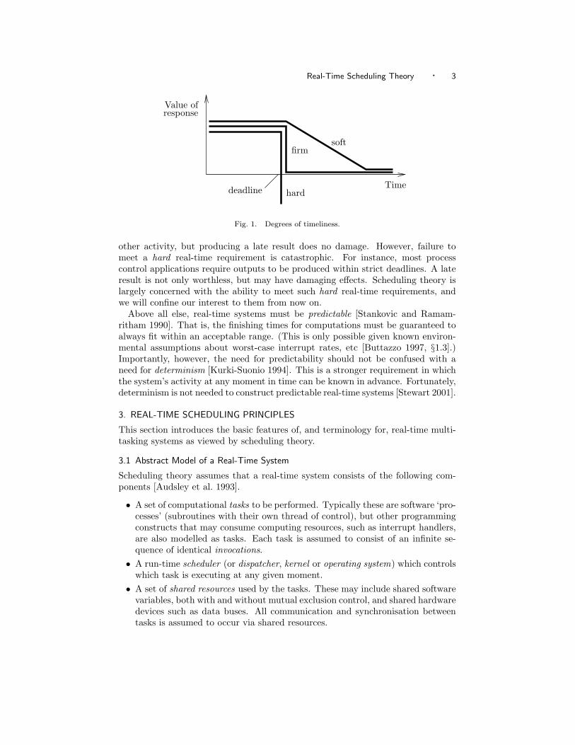
Particular timing requirements can be categorised as either soft, firm or hard asshown in Figure 1 [Buttazzo 1997, p. 231]. Soft real-time calculations may stillproduce useful results even after their timing requirement is missed. For example,a program to calculate tomorrow’s weather forecast may have a nominal deadlinein the early evening. Missing this deadline is not catastrophic, but the value ofthe calculation decreases as the following day draws nearer, and the result becomesworthless if it is not completed until tomorrow lunchtime. Failure to meet a firmreal-time requirement is wasteful but not harmful. For instance, a database querybecomes valueless after the user’s patience is exhausted and he moves on to some

Real-Time Scheduling Theory · 3

Value of

Time

softfirm

hard

response

deadline

Fig. 1. Degrees of timeliness.

other activity, but producing a late result does no damage. However, failure tomeet a hard real-time requirement is catastrophic. For instance, most processcontrol applications require outputs to be produced within strict deadlines. A lateresult is not only worthless, but may have damaging effects. Scheduling theory islargely concerned with the ability to meet such hard real-time requirements, andwe will confine our interest to them from now on.

Above all else, real-time systems must be predictable [Stankovic and Ramam-ritham 1990]. That is, the finishing times for computations must be guaranteed toalways fit within an acceptable range. (This is only possible given known environ-mental assumptions about worst-case interrupt rates, etc [Buttazzo 1997, §1.3].)Importantly, however, the need for predictability should not be confused with aneed for determinism [Kurki-Suonio 1994]. This is a stronger requirement in whichthe system’s activity at any moment in time can be known in advance. Fortunately,determinism is not needed to construct predictable real-time systems [Stewart 2001].

3. REAL-TIME SCHEDULING PRINCIPLES

This section introduces the basic features of, and terminology for, real-time multi-tasking systems as viewed by scheduling theory.

3.1 Abstract Model of a Real-Time System

Scheduling theory assumes that a real-time system consists of the following com-ponents [Audsley et al. 1993].

• A set of computational tasks to be performed. Typically these are software ‘pro-cesses’ (subroutines with their own thread of control), but other programmingconstructs that may consume computing resources, such as interrupt handlers,are also modelled as tasks. Each task is assumed to consist of an infinite se-quence of identical invocations.

• A run-time scheduler (or dispatcher, kernel or operating system) which controlswhich task is executing at any given moment.

• A set of shared resources used by the tasks. These may include shared softwarevariables, both with and without mutual exclusion control, and shared hardwaredevices such as data buses. All communication and synchronisation betweentasks is assumed to occur via shared resources.

4 · C. J. Fidge

dispatching

ready queue

termination

preemptionexecution

activation

scheduling

suspension/blocking

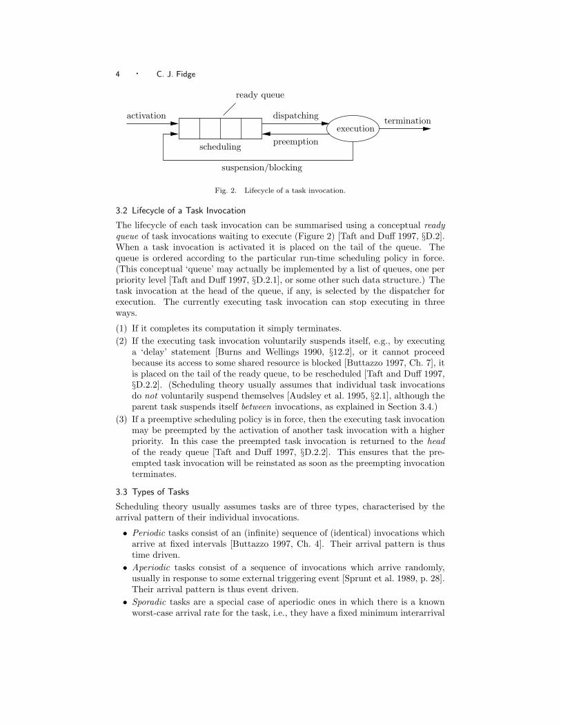
Fig. 2. Lifecycle of a task invocation.

3.2 Lifecycle of a Task Invocation

The lifecycle of each task invocation can be summarised using a conceptual readyqueue of task invocations waiting to execute (Figure 2) [Taft and Duff 1997, §D.2].When a task invocation is activated it is placed on the tail of the queue. Thequeue is ordered according to the particular run-time scheduling policy in force.(This conceptual ‘queue’ may actually be implemented by a list of queues, one perpriority level [Taft and Duff 1997, §D.2.1], or some other such data structure.) Thetask invocation at the head of the queue, if any, is selected by the dispatcher forexecution. The currently executing task invocation can stop executing in threeways.

(1) If it completes its computation it simply terminates.(2) If the executing task invocation voluntarily suspends itself, e.g., by executing

a ‘delay’ statement [Burns and Wellings 1990, §12.2], or it cannot proceedbecause its access to some shared resource is blocked [Buttazzo 1997, Ch. 7], itis placed on the tail of the ready queue, to be rescheduled [Taft and Duff 1997,§D.2.2]. (Scheduling theory usually assumes that individual task invocationsdo not voluntarily suspend themselves [Audsley et al. 1995, §2.1], although theparent task suspends itself between invocations, as explained in Section 3.4.)

(3) If a preemptive scheduling policy is in force, then the executing task invocationmay be preempted by the activation of another task invocation with a higherpriority. In this case the preempted task invocation is returned to the headof the ready queue [Taft and Duff 1997, §D.2.2]. This ensures that the pre-empted task invocation will be reinstated as soon as the preempting invocationterminates.

3.3 Types of Tasks

Scheduling theory usually assumes tasks are of three types, characterised by thearrival pattern of their individual invocations.

• Periodic tasks consist of an (infinite) sequence of (identical) invocations whicharrive at fixed intervals [Buttazzo 1997, Ch. 4]. Their arrival pattern is thustime driven.

• Aperiodic tasks consist of a sequence of invocations which arrive randomly,usually in response to some external triggering event [Sprunt et al. 1989, p. 28].Their arrival pattern is thus event driven.

• Sporadic tasks are a special case of aperiodic ones in which there is a knownworst-case arrival rate for the task, i.e., they have a fixed minimum interarrival


1: arrival : Time;

..

.

2: arrival := Clock; -- first arrival time

3: loop -- loop forever

4: delay until arrival; -- suspend task until arrival time

5: ‘action’; -- code for task invocation

6: -- deadline: arrival + D

7: arrival := arrival + T ; -- determine next arrival time

8: end loop;

Fig. 3. A typical periodic task expressed in Ada.

time [Sprunt et al. 1989, p. 28].

Since aperiodic tasks may arrive with an unknown rapidity, it is impossible toguarantee that any given task set can handle them quickly enough. Hard real-timescheduling theory therefore assumes that task sets consist of periodic and sporadictasks only. (Some extensions to the theory also allow for hybrid forms of task suchas ‘sporadically periodic’ ones [Audsley et al. 1993] [Tindell et al. 1994].)

Other computational activities are modelled using these task types. In particu-lar, interrupt handlers are modelled as sporadic tasks, with the occurrence of thecorresponding interrupt as the triggering event, and scheduler and communicationoverheads can be modelled explicitly as tasks. Furthermore, because schedulabil-ity analysis typically assumes a worst-case scenario in which sporadic tasks arriveas quickly as possible, i.e., once per their minimum interarrival time, the analysiseffectively assumes that the whole task set consists of periodic tasks only.

Individual task invocations may be further categorised by their willingness to bepreempted while executing [Buttazzo 1997, §2.3.1].

• Non-preemptive task invocations execute to completion without interruptiononce started.

• Preemptive task invocations can be temporarily preempted during their execu-tion by the arrival of a higher-priority invocation. (Preemptive task invocationscan temporarily prevent themselves from being preempted by locking a sharedresource, as explained in Section 4.4.)

3.4 Typical Periodic Task Code

As a concrete illustration of a task, Figure 3 shows the programming language codethat preemptive scheduling theory assumes is used to implement a typical periodictask [Stoyenko and Baker 1994, pp. 103–4]. It consists of an infinite loop (lines 3to 8) where some ‘action’ is performed at each iteration (line 5). Each execution ofthis action represents one task invocation. The action itself is application-specific,but typically involves sampling an input, processing data, and/or writing an output.

The remaining statements are used to control the task’s periodicity. A time-valued variable arrival is declared to hold the (earliest) time at which the nexttask invocation may begin (line 1). It is initialised with the time the task begins(line 2), or some specific absolute time. Within the loop, the start of each taskinvocation is then delayed until the time represented by arrival (line 4). Note

6 · C. J. Fidge

��

��

��

��

��

interarrival time (or period) T

(relative) deadline D

absolutedeadline

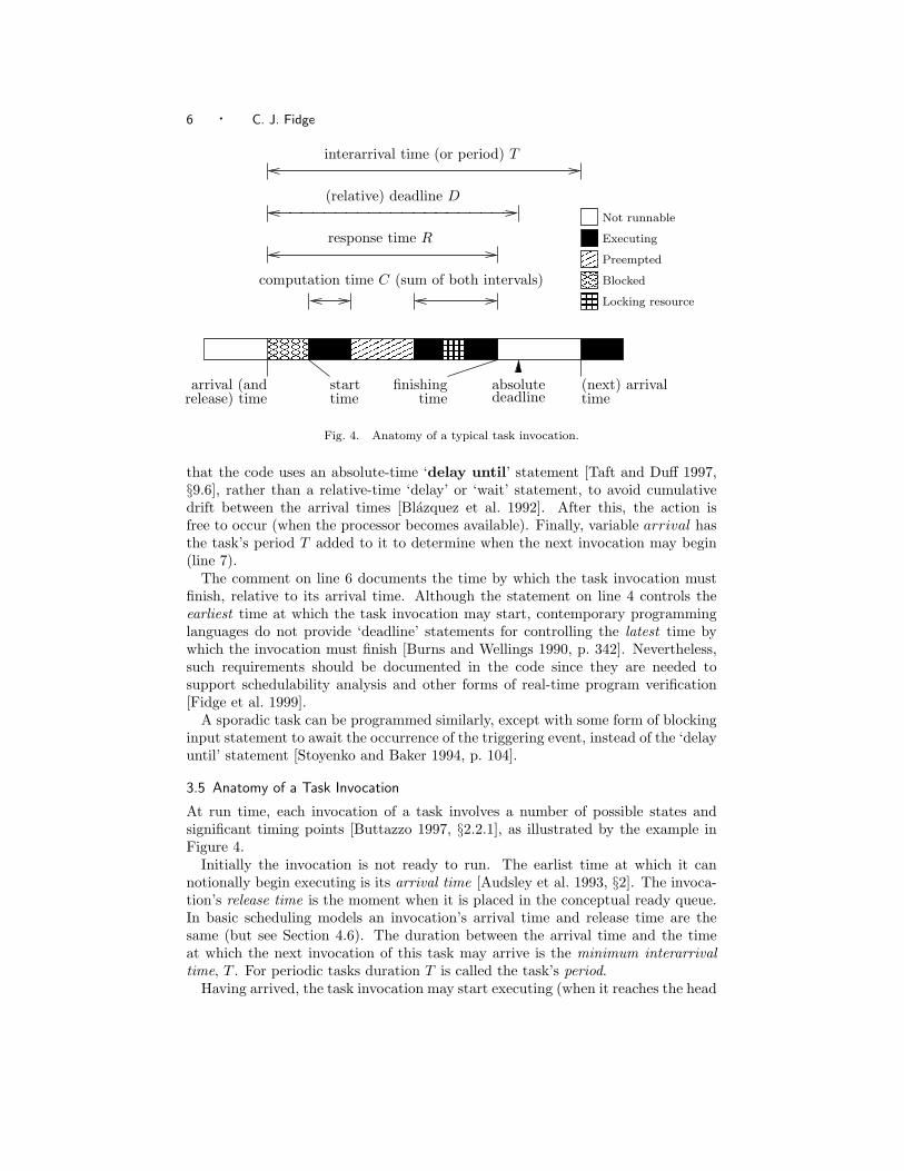
computation time C (sum of both intervals) Blocked

Not runnable

Executing

Preempted

Locking resource

response time R

starttime

finishingtime

(next) arrivaltimerelease) time

arrival (and

Fig. 4. Anatomy of a typical task invocation.

that the code uses an absolute-time ‘delay until’ statement [Taft and Duff 1997,§9.6], rather than a relative-time ‘delay’ or ‘wait’ statement, to avoid cumulativedrift between the arrival times [Blazquez et al. 1992]. After this, the action isfree to occur (when the processor becomes available). Finally, variable arrival hasthe task’s period T added to it to determine when the next invocation may begin(line 7).

The comment on line 6 documents the time by which the task invocation mustfinish, relative to its arrival time. Although the statement on line 4 controls theearliest time at which the task invocation may start, contemporary programminglanguages do not provide ‘deadline’ statements for controlling the latest time bywhich the invocation must finish [Burns and Wellings 1990, p. 342]. Nevertheless,such requirements should be documented in the code since they are needed tosupport schedulability analysis and other forms of real-time program verification[Fidge et al. 1999].

A sporadic task can be programmed similarly, except with some form of blockinginput statement to await the occurrence of the triggering event, instead of the ‘delayuntil’ statement [Stoyenko and Baker 1994, p. 104].

3.5 Anatomy of a Task Invocation

At run time, each invocation of a task involves a number of possible states andsignificant timing points [Buttazzo 1997, §2.2.1], as illustrated by the example inFigure 4.

Initially the invocation is not ready to run. The earlist time at which it cannotionally begin executing is its arrival time [Audsley et al. 1993, §2]. The invoca-tion’s release time is the moment when it is placed in the conceptual ready queue.In basic scheduling models an invocation’s arrival time and release time are thesame (but see Section 4.6). The duration between the arrival time and the timeat which the next invocation of this task may arrive is the minimum interarrivaltime, T . For periodic tasks duration T is called the task’s period.

Having arrived, the task invocation may start executing (when it reaches the head


of the conceptual ready queue). However, due to competition for the processorand other shared resources this may not happen immediately. In Figure 4 theinvocation’s start time is delayed because the task is initially blocked by a lower-priority task (Section 4.4).

Once started, the task invocation will execute until its computation is completedat its finishing time. A non-preemptible task invocation will execute without inter-ruption. However, for a preemptible task, as shown in Figure 4, the task invocationmay be temporarily preempted by a higher-priority invocation. The sum of theintervals during which the task invocation is executing, excluding blocking andpreemption, is its computation time, C. While executing, the task may also lockshared resources (Section 4.4) which may impact upon the progress of other tasks.

As well as its period, the programmer must supply a deadline, D, for each task,within which all of its invocations must finish executing. The deadline is specifiedrelative to the arrival time of the task invocation [Tindell et al. 1994, p. 149],and thus defines the corresponding absolute deadline. If the relative deadline for aperiodic task is left unstated it is usually assumed to equal the task’s period. Thepurpose of the deadline is to constrain the acceptable finishing times for the taskinvocation. The duration between the task invocation’s arrival and finishing times(including intervals of blocking and preemption) is called the invocation’s responsetime, R, which is required not to exceed the relative deadline D. Variability in thetask’s response time from one invocation to the next is known as (finishing time)jitter [Giering III and Baker 1994, p. 55].

3.6 A Taxonomy of Scheduling Algorithms

Numerous algorithms for scheduling real-time tasks exist. Broadly speaking, how-ever, they can be categorised as follows [Buttazzo 1997, §2.3.1].

• Static scheduling algorithms require the programmer to define the entire sched-ule prior to execution. At run time this pre-determined schedule is then usedto guide a simple task dispatcher. Cyclic executives are one way to programstatic task scheduling [Burns and Wellings 1990, pp. 352–354].

• Dynamic scheduling algorithms make decisions about which task to execute atrun time, based on the priorities of the task invocations in the ready queue.They require a more complex run-time dispatcher or scheduler. Such algorithmscan be further categorised into those based on fixed and changeable priorities.◦ Fixed-priority scheduling algorithms statically associate a priority with

each task in advance. This can be done arbitrarily by the programmer, oraccording to some consistent policy. Two well-known policies for fixed pri-ority assignment are Deadline Monotonic Scheduling, in which tasks withshorter deadlines are allocated higher priorities [Tindell 2000], and RateMonotonic Scheduling, in which tasks with shorter periods are allocatedhigher priorities [Briand and Roy 1999].

◦ Dynamic-priority scheduling algorithms determine the priorities of eachtask invocation at run time. Typically this requires a more complex run-time scheduler than fixed-priority scheduling. Two methods of dynamicpriority assignment are Earliest Deadline First, in which the ready taskinvocation with the earlist upcoming deadline is given highest priority [Liuand Layland 1973], and Least Laxity, in which the ready task invocation

8 · C. J. Fidge

��

��

��

��

��

��

��

151050 20

Activity A

Activity B

Activity C

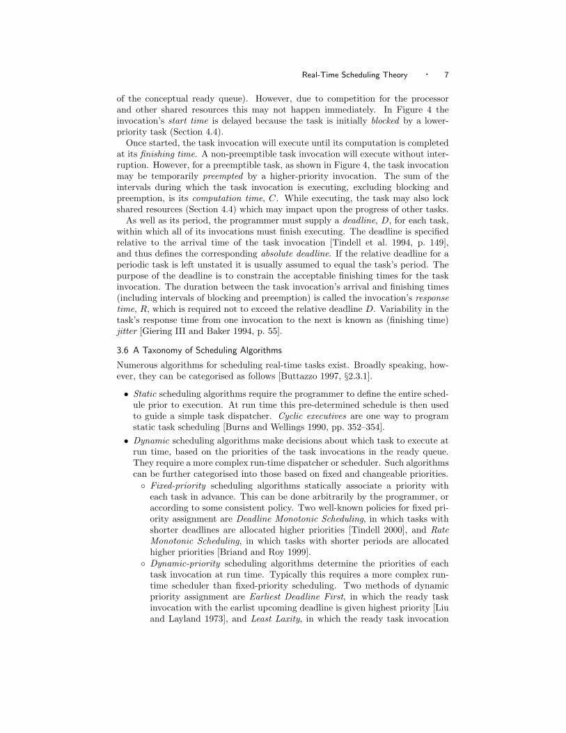
IdleExecutingNot runnable

major cycle

minor cycle

Fig. 5. A static schedule.

with the smallest difference between its upcoming deadline and (estimated)remaining computation time is given highest priority [Jones et al. 1996].

3.7 Task Scheduling Examples

To illustrate the difference between the scheduling policies mentioned in Section 3.6,this section presents four different ways of scheduling sets of computational require-ments, and summarises their advantages and disadvantages.

3.7.1 Static Scheduling. Consider three distinct activities, A, B and C, whichinvolve monitoring and responding to external events. Their rates of occurrenceare determined by the need to respond to such events in a timely manner. Ina 20 millisecond interval, activity A must occur four times and requires up to1 millisecond of processor time at each occurrence. In the same interval activity Bmust occur once and requires 7 milliseconds of processor time, and activity C mustoccur twice and requires 3 milliseconds of processor time at each occurrence.

To meet these requirements using static scheduling, the programmer is obliged toallocate activities to each unit of processor time [Burns and Wellings 1990, pp. 352–354]. One such static schedule is shown in Figure 5. Having devised this schedule,the programmer would then encode it as a cyclic executive program which iteratesevery 20 milliseconds and in each iteration performs the three activities in the se-quence shown in the figure [Kalinsky 2001] [Tindell 2000, p. 21] [Burns and Wellings1990, p. 178]. In this case, the program has a major cycle of 20 milliseconds, afterwhich the whole schedule repeats, and a minor cycle of 1 millsecond, into whicheach occurrence of an activity must fit [Locke 1992, §2].

Static scheduling is a simple approach that has a number of advantages.

+ It produces programs that are entirely deterministic. It is possible to knowwhich task is executing at any given time.


+ It does not require a run-time operating system to schedule the activities [Locke1992, §2.1]. The interleaving of activities is ‘hardwired’ into the applicationprogram’s code.

+ For control-system applications it exhibits low jitter, i.e., the separate occur-rences of each activity are always evenly spaced in time [Locke 1992, p. 43].

However, despite these advantages, static scheduling also has numerous draw-backs.

− Static schedules are rigid and difficult to construct [Kalinsky 2001]. They pro-vide determinism (i.e., the ability to know at every instant which activity isexecuting) whereas only predictability (i.e., the ability to know that activitieswill finish their computations in time) is required in a real-time system [Locke1992, p. 45].

− The approach supports periodic activities only. Responding to infrequentevents must be achieved by ‘polling’ for their occurrence. Such programs canbe computationally inefficient [Tindell 2000, p. 21]. For instance, activity Awas scheduled frequently in Figure 5, on the assumption that it must respondrapidly to its triggering event. If, however, this event occurs infrequently, thenmost of A’s occurrences will do nothing [Burns and Wellings 1990, p. 179].

− Another potential source of inefficiency is the need to fit all activities intocommon multiples of the major and minor cycles [Tindell 2000, p. 21]. In theschedule devised in Figure 5, some cycles were left idle because the activitiesdid not fit neatly.

− If an activity does not fit exactly into the schedule, it may be necessary torewrite its code to make it fit [Tindell 2000, p. 22]. In Figure 5, for instance,the occurrence of activity B, which required 7 milliseconds, was split into twoparts of duration 4 and 3 milliseconds, respectively. The programmer mustensure that the activity’s state is properly saved at the end of the first part andreloaded at the beginning of the second. Such code is awkward to develop andexpensive to maintain—any changes to the schedule may mean rewriting eachactivity’s code.

− The cyclic executive program which implements a static schedule is inherentlymonolithic. In it, code from unrelated activities is mixed together—the pro-gram’s layout is unrelated to the application’s structure. This makes the pro-gram difficult to design, prove correct, and maintain [Burns and Wellings 1990,p. 179]. (Although the concurrency constructs of a programming language likeAda can be used to build static schedules [Baker and Shaw 1989], this is stillawkward and not an efficient use of these constructs.)

− Cyclic executive programs are unstable when an activity overruns its allottedprocessor time [Locke 1992, p. 42], e.g., due to the late arrival of some essentialdata from the environment. In this case, whichever activity appears next in theschedule will suffer the consequences of the overrun, regardless of its importanceto the overall application. Thus, the failure of an activity of low importancecan have a negative impact on a highly important one.

For these reasons, static scheduling is no longer advocated as a way of programmingembedded real-time systems [Locke 1992]. Multi-tasking solutions instead support

10 · C. J. Fidge

��

��

��

��

��

0 205 10 15

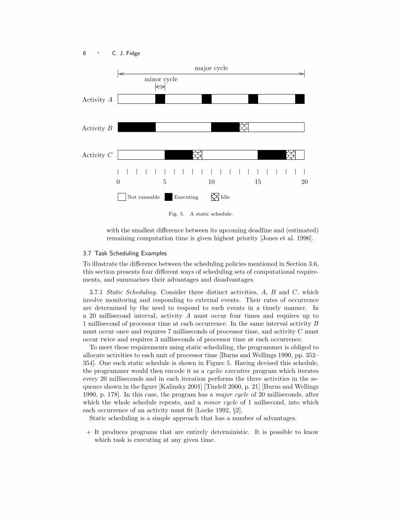
ExecutingNot runnable

Task H

Task M

Task L

Blocked Deadlines

Fig. 6. Non-preemptive fixed-priority scheduling.

separation of activities into distinct tasks, which can be developed and maintainedin isolation, while still supporting timing predictability of the whole task set, thanksto the schedulability testing principles described in Section 4 below.

3.7.2 Non-Preemptive Fixed-Priority Scheduling. Consider three distinct tasks,H, M , and L, with programmer-allocated priorities of high, medium and low, re-spectively. Following its arrival an invocation of task H requires up to 4 millisecondsof processor time and has a deadline of 10 milliseconds (relative to its arrival). Uponarrival an invocation of task M requires up to 7 milliseconds of processor time andhas a deadline of 12 milliseconds. Task L’s invocations require up to 6 millisecondsand have a deadline of 19 milliseconds. (This set of tasking requirements is notmeant to be directly comparable to the set of activities in Section 3.7.1.) For thepurposes of illustration, assume that an invocation of task L arrives at time 1, aninvocation of task M arrives at time 5, and an invocation of task H arrives attime 9.

Under these cirumstances, Figure 6 shows how these three task invocations wouldbe executed under a non-preemptive, fixed-priority scheduling policy. At time 1task L’s invocation arrives and begins executing. Task M ’s invocation arrives attime 5 but must wait until time 7, when task L’s invocation finishes, before it canstart. Similarly, although an invocation of task H arrives at time 9, it must waituntil task M ’s invocation finishes at time 14 before it starts. Despite these delays,all three task invocations meet their respective deadlines.

Non-preemptive scheduling has several distinct advantages.

+ It offers a simple programming paradigm which can be implemented in a pro-gramming language such as Ada using a small number of basic tasking features[Burns and Wellings 1996b]. This is achieved as a form of coroutining, in whicheach task executes without interruption until it voluntarily suspends itself andreturns control to the dispatcher.

+ Unlike static scheduling, a multi-tasking program allows individual tasks to beprogrammed separately, and the overall task set can be defined to mirror thestructure of the particular application.


��

��

��

��

��

0 5 10 15 20

Not runnable Executing Preempted

Task H

Task M

Task L

Deadlines

Fig. 7. Preemptive fixed-priority scheduling.

+ Task sets implemented under a fixed-priority scheduling policy can be formallyanalysed for schedulability (Section 4).

+ It has been suggested [Burns and Wellings 1996b, §2] that the simple behaviourof such systems is compatible with the Level A (uppermost) software require-ments of the DO-178B standard for airborne systems certification [RTCA, Inc.1992].

The principal disadvantages of non-preemptive scheduling are as follows.

− It is unresponsive to changes in the set of ready tasks or to inputs from theenvironment, due to the inability to stop a task invocation once it starts. Thiscan unnecessarily delay high-priority tasks. In Figure 6, for instance, task H’sinvocation was forced to wait for a considerable interval following its arrival forthe invocation of lower-priority task M to finish.

− More seriously, if a fault occurs, a wayward task invocation can monopolise theprocessor indefinitely. This also means that an overrunning low-priority taskcan delay a higher-priority one, so a non-preemptive schedule is unstable whenoverloaded.

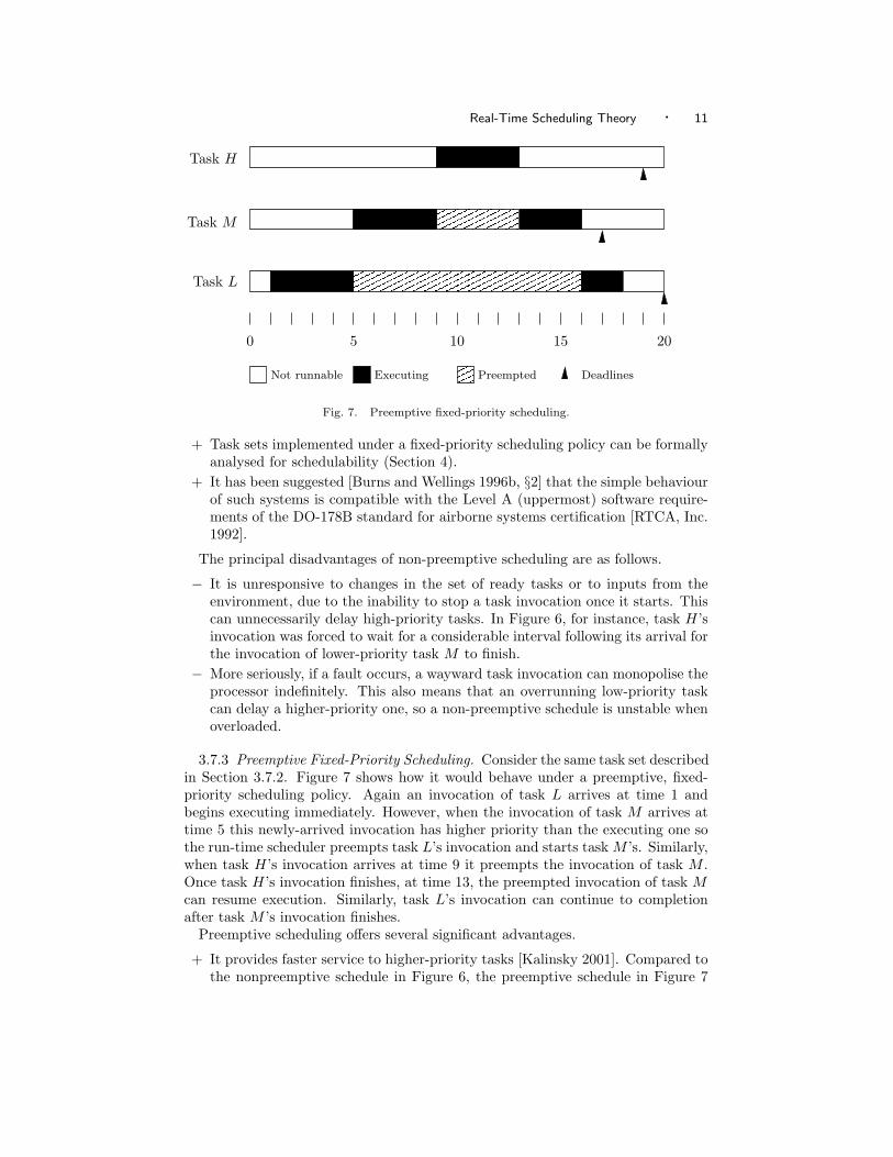
3.7.3 Preemptive Fixed-Priority Scheduling. Consider the same task set describedin Section 3.7.2. Figure 7 shows how it would behave under a preemptive, fixed-priority scheduling policy. Again an invocation of task L arrives at time 1 andbegins executing immediately. However, when the invocation of task M arrives attime 5 this newly-arrived invocation has higher priority than the executing one sothe run-time scheduler preempts task L’s invocation and starts task M ’s. Similarly,when task H’s invocation arrives at time 9 it preempts the invocation of task M .Once task H’s invocation finishes, at time 13, the preempted invocation of task Mcan resume execution. Similarly, task L’s invocation can continue to completionafter task M ’s invocation finishes.

Preemptive scheduling offers several significant advantages.

+ It provides faster service to higher-priority tasks [Kalinsky 2001]. Compared tothe nonpreemptive schedule in Figure 6, the preemptive schedule in Figure 7

12 · C. J. Fidge

significantly reduces the response time for task H’s invocation (at the expenseof the lower-priority task invocations). Preemptive scheduling thus respects thepriority ordering defined by the programmer.

+ The application programmer does not need to do anything to achieve contextswitches. The run-time operating system determines when context switchesmust occur and effects them. Thus the application program code is simplerand easier to maintain.

+ Unlike static scheduling, there is no requirement in preemptive scheduling thattask periods must be based on harmonic values [Tindell 2000]. Nor is there anyrequired relationship between a task’s timing characteristics and its priority.(Deadline and rate monotonic priority allocations can be used if such a relation-ship is desired, but this is not necessary [Audsley et al. 1995].) In fixed-prioritypreemptive scheduling the programmer is free to choose any combinations oftask priorities, periods and deadlines.

+ Numerous commercial Real-Time Operating Systems are now available to sup-port preemptive scheduling, many of which have been proven highly trustworthyand acceptably efficient [Embedded Systems Programming 2001, pp. 28–51].

+ Schedulability tests for proving that a given preemptive task set will alwaysmeet all its deadlines are now well established, as explained below (Section 4).

+ Under transient overloads, preemptively scheduled systems are stable. Thatis, the lowest priority task invocations will miss their deadlines, rather thanhigher-priority ones. In particular, both deadline and rate monotonic priorityallocations for sets of independent tasks are stable when overloaded [Gomaa1993, p. 124] [Audsley et al. 1992].

However, fixed-priority preemptive scheduling has some disadvantages for em-bedded control systems.

− A complex run-time operating system is required to support preemptive schedul-ing [Kalinsky 2001]. Context switching may take a significant time (this over-head was ignored in Figure 7), and a significant amount of memory may berequired to store the state of preempted task invocations.

− Preemptive scheduling can introduce higher degrees of jitter than a static sched-ule. For instance, the finishing time of invocations of task L above, relative toits arrival time, can vary widely depending on whether the invocation is pre-empted or not. (Jitter can be minimised by appropriate structuring of the taskset [Locke 1992, §3.2], or by introducing offsets [Bate and Burns 1999, §3.2],however.)

− It is not clear how a preemptively scheduled system can be certified safe usingexisting guidelines such as avionics standard DO-178B [RTCA, Inc. 1992]. Suchstandards often require exhaustive testing of all possible control-flow pathsthrough a program. This requirement is inappropriate for a preemptive systemin which control flow between tasks is determined dynamically at run time.(Instead, reliance should be put on scheduling theory to help prove timingcorrectness, rather than just testing.)

An additional disadvantage perceived by some programmers of critical systems isthe fact that preemptive scheduling does not offer the same degree of determinism


��

��

��

��

��

��

0 5 10 15 20


Task A

Task B

Task C

Deadlines

Fig. 8. Preemptive dynamic-priority scheduling.

as static scheduling. Nevertheless, determinism is not normally required in practice,only predictablility [Locke 1992, p. 45], and this can be guaranteed using schedulingtheory.

3.7.4 Preemptive Dynamic-Priority Scheduling. Again, consider the same taskset described in Section 3.7.2, except that here we label the tasks A, B and C,since they do not have statically-associated priorities. Figure 8 shows how thesetasks would behave under a particular dynamic-priority scheduling policy, EarliestDeadline First. When task B’s invocation arrives at time 5 the run-time schedulercompares its absolute deadline of 17 with the deadline of 20 for the currently-executing invocation of task C, and switches control to the invocation with theearlier deadline. When the invocation of task A arrives at time 9, its later deadlineof 19 means that the invocation of task B is not preempted. At time 12 task B’sinvocation finishes and the run-time scheduler starts the invocation with the earliestdeadline, in this case task A’s.

The major advantage of dynamic-priority preemptive scheduling is as follows.

+ In theory, ignoring implementation overheads, it offers the best possible guaran-tee that tasks will meet their deadlines, since it always ensures that processingpower is dedicated to the task invocation with the most urgent need [Liu andLayland 1973, p. 186] [Giering III and Baker 1994, p. 55].

However, dynamic-priority preemptive scheduling has the following disadvan-tages.

− It incurs even higher run-time overheads than fixed-priority scheduling, sincethe priorities of all tasks in the ready queue must be recalculated each time atask arrives or finishes.

− It is unstable under transient overload in the sense that it is difficult to predictwhich task will miss its deadline first.

These practical disadvantages tend to outweigh dynamic-priority scheduling’s the-oretical advantages [Liu and Layland 1973] [Jones et al. 1996] and it is thus lesscommon in practice than fixed-priority scheduling.

14 · C. J. Fidge

��

��

��

��

��

��

1050 15

CPU

IOP

HoutHin Lin

Hproc Lproc

Lout

Hi-pri task executing Lo-pri task executing Messages

transaction H’s response time

transaction L’s response time

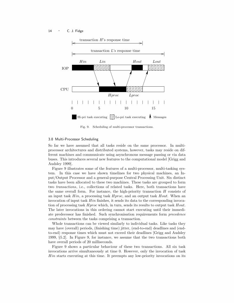
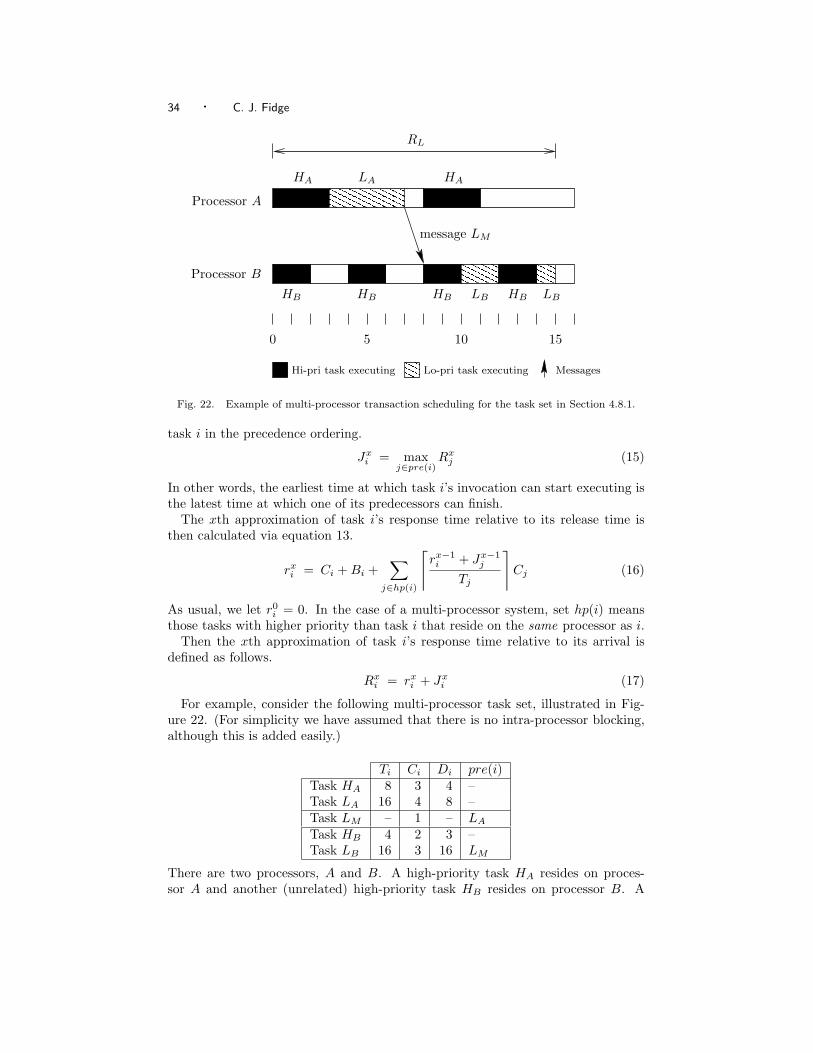
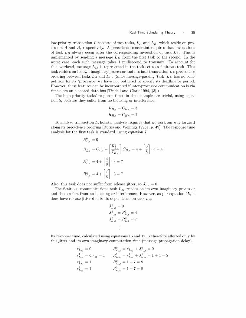
Fig. 9. Scheduling of multi-processor transactions.

3.8 Multi-Processor Scheduling

So far we have assumed that all tasks reside on the same processor. In multi-processor architectures and distributed systems, however, tasks may reside on dif-ferent machines and communicate using asynchronous message passing or via databuses. This introduces several new features to the computational model [Grigg andAudsley 1999].

Figure 9 illustrates some of the features of a multi-processor, multi-tasking sys-tem. In this case we have shown timelines for two physical machines, an In-put/Output Processor and a general-purpose Central Processing Unit. Six distincttasks have been allocated to these two machines. These tasks are grouped to formtwo transactions, i.e., collections of related tasks. Here, both transactions havethe same overall form. For instance, the high-priority transaction H consists ofan input task Hin, a processing task Hproc, and an output task Hout. When aninvocation of input task Hin finishes, it sends its data to the corresponding invoca-tion of processing task Hproc which, in turn, sends its results to output task Hout.The later invocations in this ordering cannot start executing until their immedi-ate predecessor has finished. Such synchronisation requirements form precedenceconstraints between the tasks comprising a transaction.

Whole transactions can be viewed similarly to individual tasks. Like tasks theymay have (overall) periods, (finishing time) jitter, (end-to-end) deadlines and (end-to-end) response times which must not exceed their deadlines [Grigg and Audsley1999, §5.2]. In Figure 9, for instance, we assume that the two transactions bothhave overall periods of 20 milliseconds.

Figure 9 shows a particular behaviour of these two transactions. All six taskinvocations arrive simultaneously at time 0. However, only the invocation of taskHin starts executing at this time. It preempts any low-priority invocations on its


processor, and the other tasks in transaction H cannot begin until it has finisheddue to their precedence constraints. At time 4 Hin’s invocation finishes and sendsits data to the other processor. We assume in Figure 9 that all inter-processorcommunication takes 1 millisecond. This means that the invocation of task HProccan start executing at time 5. Similarly, task Hout’s invocation starts executing attime 11, once it has received a message from HProc’s invocation.

Low-priority transaction L’s behaviour in Figure 9 is similar to that of the high-priority one, except that it suffers interference from transaction H. For instance, theinvocation of task Lin cannot begin until time 4, due to preemption from task Hin’sinvocation. Also, even though Lproc’s invocation has its precedence constraintsatisfied at time 8, by the arrival of the message from Lin’s invocation, it muststill wait for the invocation of task Hproc to finish. Thus schedulability analysisfor tasks in multi-processor systems is especially complex because it depends notonly on those tasks that reside on the same processor, but also on the arrival ofmessages from tasks on other processors.

The run-time sequencing of the nth and (n + 1)th tasks in a transaction’s prece-dence ordering can be enforced in three different ways. Recall that all task invoca-tions comprising a particular transaction invocation are deemed to arrive simulta-neously.

(1) If both tasks reside on the same processor then the (n+1)th task can simply begiven a lower priority than the nth to achieve the necessary execution ordering.

(2) If the tasks reside on different processors then the ordering can be enforcedby appropriate communication mechanisms. In a distributed system, messagepassing would be used and the nth task’s invocation will finish by sendinga message to the (n + 1)th, and the (n + 1)th task’s invocation will beginwith a (blocking) input action which awaits the message. In a multi-processorarchitecture, communication over a data bus or a system-wide interrupt canbe used to signal completion of a task invocation between machines [Falardeau1994, §4.1.3.1].

(3) Alternatively, precedence constraints across processors can be enforced by theuse of offsets which introduce a constant shift of a task’s arrival times fromwhole multiples of its period [Bate and Burns 1999]. The (n+1)th task invoca-tion in a precedence ordering is given an offset at least as great as the worst-caseresponse time of the nth. This not only ensures that the precedence ordering isrespected, but it also allows the earlier task’s invocation to communicate withthe later one merely by writing to a shared data area, confident that the latertask’s invocation will not attempt to read the data too early. (However, usingoffsets is possible only if there is tight synchronisation of clocks on the differentprocessors [Falardeau 1994, p. 68].)

Typically, therefore, the first task in a transaction will arrive periodically, whereasthe starting times of later task invocations in the precedence ordering depend on theresponse times of earlier ones [Falardeau 1994, §3.4.3]. Unfortunately, this meansthat the (starting and finishing time) jitter of tasks [Grigg and Audsley 1999] iscumulative along the precedence ordering. Thus the response-time variability ofsuccessive invocations of task Hout from Figure 9 could be very high. Since highjitter is usually unacceptable in control systems [Bate and Burns 1999], a way isneeded to reduce it for multi-processor systems. This can usually be achieved by

16 · C. J. Fidge

Γ The set of task identifiersn The number of tasks in set Γ

hp(i) The set of tasks with higher priority than task ihep(i) The set of tasks with higher or equal priority to task i

lp(i) The set of tasks with lower priority than task ipre(i) The set of tasks preceding task i in a transaction

locks(k, i) The set of resources used by task k with ceiling priority i or higher

Ti Minimum interarrival time, or periodDi Deadline (relative to arrival)Ci Worst-case computation timeBi Worst-case blocking timeOi Offset from arrival time

ci,S Worst-case computation time while locking resource S

9>>>>>>=>>>>>>;Given for eachtask i

Ri Worst-case response time relative to arrivalri Worst-case response time relative to releaseIi Worst-case interferenceJi Worst-case release jitter

Wi(t) Processor workload at time t

9>>>>=>>>>;Calculatedfor eachtask i

Table 1. Symbols used in schedulability equations.

introducing offsets into the task set [Tindell and Clark 1994]. For instance, if weassume that Figure 9 is the worst-case behaviour for invocations of these tasks, thenwe could define an offset of 11 milliseconds for task Hout. Thus its first invocationwould arrive at time 11, its second at time 31 and so on. This means that even ifinvocations of tasks Hin and Hproc finish earlier than the times shown in Figure 9,the invocation of task Hout will still wait until (at least) time 11 to start executing.Although this may mean that the processor may be idle more often than necessary,successive invocations of task Hout will remain evenly spaced, as is usually requiredfor input/output events in process control applications.

4. REAL-TIME SCHEDULABILITY TESTS

Although the computational model described above is in itself an aid to under-standing the dynamic behaviour of a real-time multi-tasking system, the true valueof scheduling theory is in its schedulability tests which accurately predict whethera task set will always meet its deadlines or not.

Dozens of schedulability tests have been developed for real-time multi-tasking sys-tems [Fidge 1998] but, generally speaking, they are all variants of, or derived from,three basic approaches: processor utilisation, processor workloads, and responsetime analysis (Sections 4.1, 4.2 and 4.3, respectively). Furthermore, processor util-isation measurement is effectively obsolete, having been superseded by processorworkload analysis, and workload analysis itself has proven to be equivalent to gen-eral response time analysis [Audsley et al. 1995, p. 182]. Therefore, although webriefly present processor utilisation and workload equations in Sections 4.1 and 4.2below, due to their historical significance, the major principles of schedulabilityanalysis are all covered by the response time tests detailed in Sections 4.3 to 4.8.The symbols used in the equations are shown in Table 1.


��

��

��

��

��

��

0 10 15

Task H

Task M

Executing Preempted

Task L

Deadlines

5

Not runnable

(and its second starts)L’s first invocation finishesL’s first invocation

misses its deadline

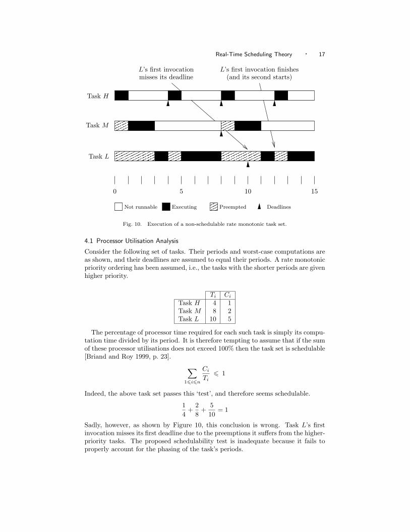
Fig. 10. Execution of a non-schedulable rate monotonic task set.

4.1 Processor Utilisation Analysis

Consider the following set of tasks. Their periods and worst-case computations areas shown, and their deadlines are assumed to equal their periods. A rate monotonicpriority ordering has been assumed, i.e., the tasks with the shorter periods are givenhigher priority.

Ti Ci

Task H 4 1Task M 8 2Task L 10 5

The percentage of processor time required for each such task is simply its compu-tation time divided by its period. It is therefore tempting to assume that if the sumof these processor utilisations does not exceed 100% then the task set is schedulable[Briand and Roy 1999, p. 23].

∑

16i6n

Ci

Ti6 1

Indeed, the above task set passes this ‘test’, and therefore seems schedulable.

14

+28

+510

= 1

Sadly, however, as shown by Figure 10, this conclusion is wrong. Task L’s firstinvocation misses its first deadline due to the preemptions it suffers from the higher-priority tasks. The proposed schedulability test is inadequate because it fails toproperly account for the phasing of the task’s periods.

18 · C. J. Fidge

To correct this, the following schedulability test [Liu and Layland 1973] wasdevised to account for any possible task phasing.

∑

16i6n

Ci

Ti6 n(2

1n − 1) (1)

The term on the right is a processor utilisation bound, expressed in terms of thenumber n of tasks. For three tasks this bound is approximately 0.78. Since the totalprocessor utilisation for our three tasks exceeds this, test 1 correctly determines thatthe task set above is not schedulable.

Unfortunately, schedulability test 1 has many limitations [Briand and Roy 1999,§2.3].

− It applies to preemptive task sets only.− It applies to rate monotonic task sets only. Tasks whose importance is not

proportional to their period cannot be accommodated.− It applies to independent, non-interacting tasks only.− All task deadlines are assumed to equal their periods. This is not acceptable for

most control applications since it allows tasks to exhibit high jitter (Section 4.7).− The processor utilisation bound rapidly converges to 0.69 as the number of tasks

increases. For large task sets, this means that the test can confirm schedula-bility only for cases of low overall processor utilisation.

Therefore, despite its historical importance, this test has been superseded by themore general tests below.

4.2 Processor Workload Analysis

Schedulability test 1 is extremely pessimistic. (Although all schedulability tests erron the side of pessimism. It is better to reject a schedulable task set than to pass anunschedulable one.) To overcome this, the following equation instead calculates thetotal computational workload on the processor at some time t, due to invocationsof tasks of priority equal to or higher than that of task i [Lehoczky et al. 1989].

Wi(t) =∑

j∈hep(i)

⌈t

Tj

⌉Cj (2)

For some task j, expression dt/Tje is the number of times this task can arrive in aninterval of duration t. (The rounding-up operator dxe returns the smallest integernot less than x.) Multiplying the number of arrivals by Cj thus defines the totalcomputational requirement by all invocations of task j in this interval. The totalworkload at time t is then just the sum for all such tasks.

To determine whether task i is schedulable, the following test then checks thatthe computational workload associated with this task and those of higher priority isnot always greater than 100% in an interval bounded by task i’s period Ti [Lehoczkyet al. 1989].

min0<t6Ti

(Wi(t)

t

)6 1 (3)

The test relies on the observation that the worst-case scenario for task i is at time 0,when it arrives simultaneously with all other tasks. If the first invocation of task i


can finish before its deadline at time Ti, then all subsequent invocations will alsobe schedulable. The test is computationally expensive due to the need to iterateover each time t, but the same result can be achieved by checking just those timesat which higher-priority tasks arrive [Lehoczky et al. 1989].

To see if task L from Section 4.1 is schedulable, we can calculate the total work-load for the three tasks at each time t, when a higher-priority task arrives duringtask L’s period, using equation 2, and divide each result by t.

WL(4)4

=(⌈

410

⌉· 5 +

⌈48

⌉· 2 +

⌈44

⌉· 1

)/4 = 2

WL(8)8

=(⌈

810

⌉· 5 +

⌈88

⌉· 2 +

⌈84

⌉· 1

)/8 =

98

WL(10)10

=(⌈

1010

⌉· 5 +

⌈108

⌉· 2 +

⌈104

⌉· 1

)/10 =

65

The minimum of these values is 98 , which exceeds 1, so test 3 confirms that the task

set in Section 4.1 is unschedulable, because the processor is always overloaded.Again, however, this test is limited to rate-monotonic, preemptive, periodic, non-

interacting tasks, with deadlines equal to their periods. The response time testsused below overcome all of these restrictions [Audsley et al. 1995, p. 182] (as dofurther extensions to workload analysis [Briand and Roy 1999]).

4.3 Basic Response Time Analysis

Both the processor utilisation and workload tests described above suffer from nu-merous restrictions. By contrast, the response time test described below is appli-cable to any fixed priority, preemptive task set, and in subsequent sections it isextended for non-preemptive scheduling and interaction between tasks.

Since the goal of schedulability analysis is to show that each task invocationfinishes before its deadline, the approach taken here is to simply calculate theworst case response time Ri for each invocation of a task i and compare it with thedeadline Di. Task i is schedulable if it passes the following trivial test [Joseph andPandya 1986].

Ri 6 Di (4)

Of course, the challenge in using test 4 is to determine the response time. All of theequations below are founded on increasingly more sophisticated ways of determiningthis value.

Firstly, we consider the case of non-interacting tasks. In this situation the re-sponse time Ri for an invocation of task i is its own worst-case computation timeCi plus the interference Ii it suffers from higher-priority tasks.

Ri = Ci + Ii (5)

(Recall that each Ci must include the run-time overheads associated with schedulingan invocation of task i. Also see Section 4.6.)

The interference term in equation 5 depends on how often higher-priority taskinvocations can preempt an invocation of task i. This can be determined, for eachhigher-priority task j, by dividing the interval of interest, Ri, by task j’s period Tj ,

20 · C. J. Fidge

��

Tj Cj

Ri

Task i

Task j

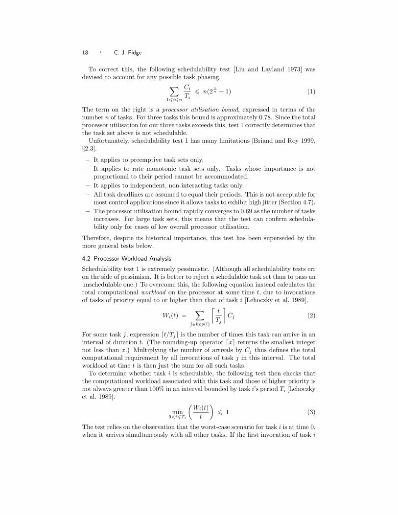
Fig. 11. Interference from higher-priority task invocations.

to obtain the number of arrivals of invocations of task j, and then multiplying thisby task j’s computation time Cj [Joseph and Pandya 1986]. For now we assumethat all task priorities are unique.

Ii =∑

j∈hp(i)

⌈Ri

Tj

⌉Cj (6)

For instance, Figure 11 shows three invocations of a high-priority task j preemptingone invocation of lower-priority task i. Thus the total interference inflicted by task jon task i is 3 times Cj .

Combining equations 5 and 6 then gives us the total calculation for the worst-case response time of a task i in a set of preemptive, fixed-priority, non-interactingtasks [Joseph and Pandya 1986].

Ri = Ci +∑

j∈hp(i)

⌈Ri

Tj

⌉Cj (7)

Note that this equation works for any fixed-priority task set, including those de-signed with either deadline or rate monotonic priority allocations, assuming uniquepriorities.

However, because the interference suffered by an invocation of task i increasesits overall response time, and equation 6 calculates the total interference in termsof the response time, equation 7 is defined recursively. Term Ri appears on bothsides of the equality. Fortunately, the equation can be solved iteratively [Audsleyet al. 1993]. We begin with an initial approximation for Ri of 0. Then the (x+1)thapproximation can be defined in terms of the xth one.

Rx+1i = Ci +

∑

j∈hp(i)

⌈Rx

i

Tj

⌉Cj

Performing this calculation will result in one of two outcomes. If Rxi converges

to a value no greater than Di then we may conclude that task i is schedulable.Alternatively, if Rx

i grows to a value exceeding Di then task i is not schedulable.For example, consider the following task set.


��

��

��

��

0 10 15

Task H

Task M

Executing Preempted

Task L

Deadlines

5

Not runnable

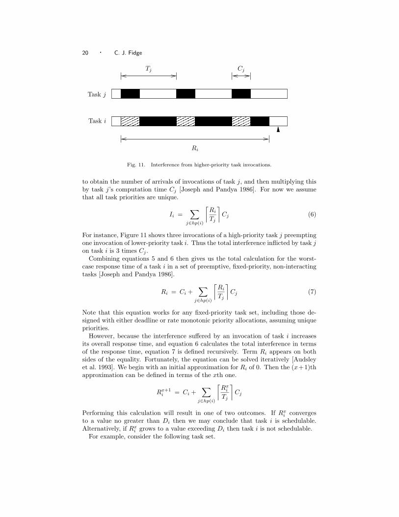
Fig. 12. Execution of the schedulable task set from Section 4.3.

Ti Ci Di

Task H 4 1 2Task M 6 2 3Task L 7 2 6

To show that this task set is schedulable we need to apply test 4 to each of thethree tasks. The response time calculation for the low-priority task L converges asfollows.

R0L = 0

R1L = CL +

⌈R0

L

TM

⌉CM +

⌈R0

L

TH

⌉CH = 2 +

⌈06

⌉· 2 +

⌈04

⌉· 1 = 2

R2L = 2 +

⌈26

⌉· 2 +

⌈24

⌉· 1 = 5

R3L = 2 +

⌈56

⌉· 2 +

⌈54

⌉· 1 = 6

R4L = 2 +

⌈66

⌉· 2 +

⌈64

⌉· 1 = 6

Since this calculated response time does not exceed deadline DL, we may concludethat task L is schedulable. Indeed, the timeline in Figure 12 shows the worst-casebehaviour of this task set, and the first invocation of task L exhibits the calculatedresponse time. Similar calculations can be performed to show that both tasks Mand H are also schedulable in this case.

4.4 Blocking on a Shared Resource

So far we have assumed that all tasks are independent, i.e., they do not interactapart from their competition for access to the processor. More realistically, tasksneed to synchronise with one another and communicate data values. To accom-

22 · C. J. Fidge

��

��

��

��

� � � � ��

��

H blocked

Blocked Lockingresource

S locked by L H needs S S unlocked by L

Not Executing Preempted

Task H

Task L

runnable

Fig. 13. Blocking by a lower-priority task.

modate this, scheduling theory’s computational model assumes that tasks residingon the same processor interact by protected access to shared resources [Buttazzo1997, §2.2.3]. (In Section 4.8 we consider message passing between tasks on dif-ferent processors.) Typically, a shared resource can be accessed by only one taskat a time. Any other task that wishes to access it at this time is blocked. Thus,by locking shared resources, low-priority task invocations can delay the progress ofhigher-priority ones.

For example, Figure 13 shows a situation where two tasks share the same re-source S. An invocation of low-priority task L starts executing first and locks theresource. High-priority task H’s invocation then arrives and preempts task L’s in-vocation. However, after executing for a short time, task H’s invocation also needsto access the shared resource. When it attempts to do so it finds that S is alreadylocked by task L. At this point task H’s invocation is blocked, i.e., it cannot executeany further, and control is returned to the low-priority task invocation. Task L’sinvocation then continues executing until it finishes using shared resource S andreleases the lock. At this point task H’s invocation is free to continue, so it imme-diately preempts task L’s invocation and accesses S.

Therefore, blocking due to lower-priority tasks can be accommodated in schedu-lability test 4 simply by adding a term for task i’s worst-case blocking time Bi tothe response time calculation [Audsley et al. 1993, §3].

Ri = Ci + Bi +∑

j∈hp(i)

⌈Ri

Tj

⌉Cj (8)

However, to know exactly what the worst-case blocking time will be for each task,we must look more closely at the way tasks may be blocked.

4.4.1 Priority Inversion. To know that a high-priority task invocation is schedu-lable, we must be able to put a bound on how long it will be blocked by lower-priorityones. However, this is not possible in general [Buttazzo 1997, §7.2].

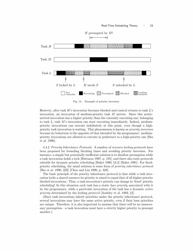
For example, Figure 14 shows the behaviour of a task set in which tasks Land H both share resource S. At first, the behaviour is the same as in Figure 13.


��

�

��

��

��

��

��


Not Executing Preemptedrunnable

S locked by L H needs S S unlocked by L

Task M

Task H

Task L

H preempted by M !

Fig. 14. Example of priority inversion.

However, after task H’s invocation becomes blocked and control returns to task L’sinvocation, an invocation of medium-priority task M arrives. Since this newly-arrived invocation has a higher priority than the currently executing one, belongingto task L, task M ’s invocation can start executing immediately. Indeed, medium-priority invocations can execute indefinitely at this point, even though a high-priority task invocation is waiting. This phenomenon is known as priority inversionbecause its behaviour is the opposite of that intended by the programmer: medium-priority invocations are allowed to execute in preference to a high-priority one [Shaet al. 1990].

4.4.2 Priority Inheritance Protocols. A number of resource locking protocols havebeen proposed for bounding blocking times and avoiding priority inversion. Forinstance, a simple but potentially inefficient solution is to disallow preemption whilea task invocation holds a lock [Buttazzo 1997, p. 185], and there also exist protocolssuitable for dynamic priority scheduling [Baker 1990, §3.2] [Baker 1991]. For fixed-priority scheduling, the usual solution is some form of priority inheritance protocol[Sha et al. 1990, §III] [Chen and Lin 1990, p. 328].

The basic principle of the priority inheritance protocol is that while a task invo-cation locks a shared resource its priority is raised to equal that of all higher-priorityblocked invocations. Thus, a task invocation’s priority can change in ‘fixed’ priorityscheduling! In this situation each task has a static base priority associated with itby the programmer, while a particular invocation of the task has a dynamic activepriority determined by the locking protocol [Audsley et al. 1993, §2].

(Since task invocations inherit priorities under the priority inheritance protocol,several invocations may have the same active priority, even if their base prioritiesare unique. Therefore, it is also important to assume that there will be no unneces-sary preemption—a task invocation must have a strictly higher priority to preemptanother.)

24 · C. J. Fidge

��

��

��

��

��

� � � � � � � � � � � � � � � ��

��

��


S locked by L S unlocked by L

push-through blockingdirect blocking(before S is needed) (although S is not used)


Task H

Task M

Task L

Fig. 15. Ceiling locking of a shared resource.

The advantage of the priority inheritance protocol is that when a low-priority taskinvocation is blocking a high-priority one, the low-priority invocation is allowed toexecute with fewer preemptions, thus allowing control to go to the high-priorityinvocation more quickly. The priority inheritance protocol both prevents priorityinversion and bounds blocking times, thus making interacting task sets analysable.A side-effect of the protocol, however, is that a task invocation may experienceblocking on a shared resource even though it does not use the resource (see theexample in Section 4.4.3 below).

4.4.3 The Ceiling Locking Protocol. In its basic form, as described above, thepriority inheritance protocol can be expensive to implement because the run-timescheduler must keep track of which task invocations hold which locks. Fortunately,a slight variant of priority inheritance has proven to be almost as effective anddramatically cheaper to implement.

In the ceiling locking protocol each shared resource has a fixed ceiling prioritywhich equals the highest base priority of any task that may access this resource[Stoyenko and Baker 1994, p. 104]. When a task invocation locks a shared re-source, it immediately raises its active priority to equal this ceiling value. (In basicpriority inheritance it would do this only when a higher-priority invocation becameblocked on the resource.) This protocol effectively prevents any task invocationfrom starting to execute until all the shared resources it needs are free [Taft andDuff 1997, §D.2.1].

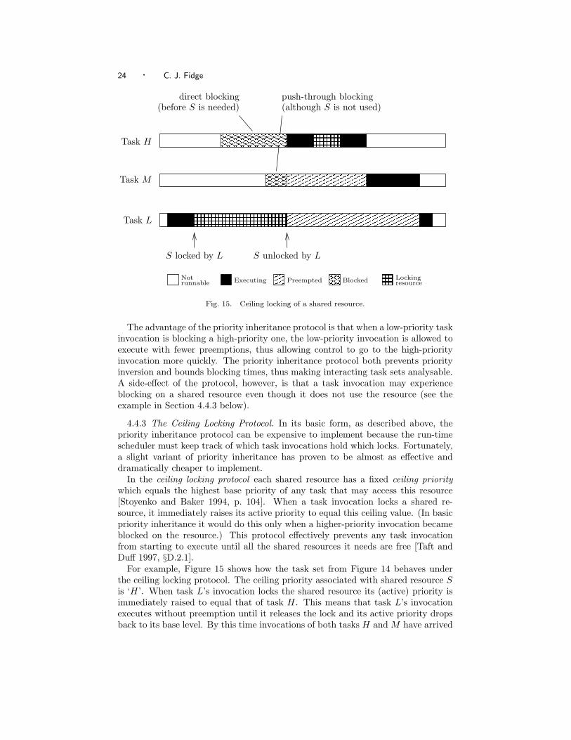
For example, Figure 15 shows how the task set from Figure 14 behaves underthe ceiling locking protocol. The ceiling priority associated with shared resource Sis ‘H’. When task L’s invocation locks the shared resource its (active) priority isimmediately raised to equal that of task H. This means that task L’s invocationexecutes without preemption until it releases the lock and its active priority dropsback to its base level. By this time invocations of both tasks H and M have arrived


and the higher-priority one gets preference. The preemption of task H’s invocationby that of task M seen in Figure 14 does not occur. The medium-priority taskmust wait for the high-priority one.

Two forms of blocking are evident in Figure 15. Task H’s invocation suffers directblocking because a lower-priority task has locked a shared resource it may need.(This occurs before the resource is actually required—in basic priority inheritancedirect blocking occurs only when an attempt is made to access the locked resource.Although ceiling locking may cause tasks to be blocked in situations where theywould not be under basic priority inheritance, the worst-case behaviour of the twoprotocols is the same.) Task M ’s invocation suffers push-through blocking , eventhough it does not use the shared resource, because task L’s invocation inheritsa higher priority while locking the resource shared with task H [Buttazzo 1997,p. 188].

Most importantly, the ceiling locking protocol has several desirable properties.

+ It is cheap to implement at run time. By raising priorities as soon as a resourceis locked, whether a higher-priority task is trying to access it or not, the protocolavoids the need to make complex scheduling decisions on the fly.

+ The way that task priorities are manipulated ensures that a task invocationcannot start until all shared resources it may need are free. This means thatno separate mutual exclusion mechanism, such as semaphores, is needed to lockshared resources [Tindell 2000]. The run-time scheduler implements both taskscheduling and resource locking using the one mechanism.

+ Since a task invocation cannot start until all resources it may need are free,run-time deadlocks caused by circular dependencies on shared resources areimpossible [Pilling et al. 1990].

+ Each task invocation can be blocked at most once, at its beginning, by a sin-gle lower-priority task. This provides the necessary bound on blocking timesneeded for analysing schedulability of interacting task sets [Audsley et al. 1995,p. 185].

For these reasons, ceiling locking is the default priority inheritance protocol in theAda 95 real-time programming language [Taft and Duff 1997, §D.1, D.3].

4.4.4 Response Time Test Incorporating Blocking Times. With an understandingof the particular resource locking protocol used, the blocking term Bi needed forequation 8 can now be defined. With the ceiling locking protocol, Bi is the longestduration of a critical section executed by any lower-priority task that accesses aresource with ceiling value i or higher [Tindell 2000]. Let locks(k, i) be the setof shared resources accessed by task k with ceiling priorities higher than or equalto task i’s priority. Let ck,S be the worst-case computation time of task k whilelocking shared resource S.

Bi = max (ck,S)k ∈ lp(i)

S ∈ locks(k, i)

(9)

For example, consider the following task set. We saw in Section 4.3 that thesethree tasks are schedulable when they are independent. However, here we assumethat tasks H and L both share a resource, and that an invocation of task L can

26 · C. J. Fidge

��

��

��

��

� � ��

��

��

��

��


25 30 35 40


Task M

Task H

Task L

M misses deadline!

Fig. 16. Missed deadlines for the task set in Section 4.4.4 due to blocking from a lower-prioritytask.

lock the shared resource for up to 1 millisecond. The blocking time column wasthen calculated used equation 9.

Ti Ci Di Bi

Task H 4 1 2 1Task M 6 2 3 1Task L 7 2 6 0

Applying test 4 using equations 8 and 9 then reveals that this task set is no longerschedulable due to the interactions between the tasks. For the medium priority taskthe calculated response time is as follows.

R0M = 0

R1M = CM + BM +

⌈R0

M

TH

⌉CH = 2 + 1 +

⌈04

⌉· 1 = 3

R2M = 2 + 1 +

⌈34

⌉· 1 = 4

R3M = 2 + 1 +

⌈44

⌉· 1 = 4

This exceeds its deadline as shown by the example in Figure 16.Importantly, notice the time scale in Figure 16. Task M does not miss a deadline

until time 33, when a particular invocation suffers both preemption from task H andblocking from task L. All previous invocations of task M meet their deadlines, in-cluding the first invocation when all three tasks arrive simultaneously. This remindsus that the behaviour of interacting tasks is much more subtle than independent


��

��

��

��

��

��

��

��

��

��

��

��

� � �

��

��

��

30 35 40 45


Task M

Task H

Task L

M misses deadline!

Blocked

Fig. 17. A missed deadline for the task set in Section 4.5 due to non-preemptive scheduling.

ones.

4.5 Response Times for Non-Preemptive Scheduling

So far we have assumed that the scheduling policy is preemptive. Non-preemptivescheduling can be analysed as a special case, using the tests for preemptive schedul-ing, by assuming that all tasks share a single resource (the processor itself) andthat they lock it for the entire duration of each invocation [Briand and Roy 1999,p. 19].

In this case the worst-case ‘blocking’ experienced by a task i is the largest com-putation time of any lower-priority task k. This represents the situation where aninvocation of task k begins executing just before an invocation of task i. Sincetask k’s invocation is not preemptible, task i’s invocation must wait for it to finish.Thus the blocking term of equation 8 can be replaced with k’s computation timeas follows.

Ri = Ci + maxk∈lp(i)

Ck +∑

j∈hp(i)

⌈Ri

Tj

⌉Cj (10)

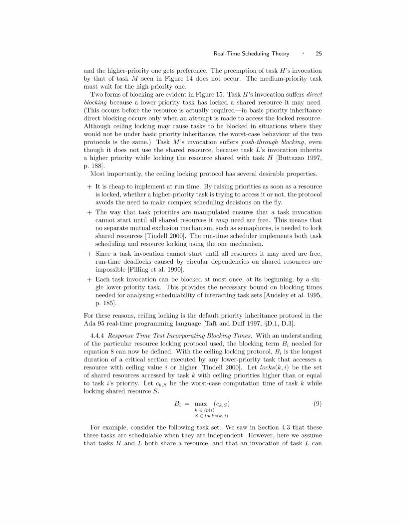
For example, consider the task set from Section 4.4.4. The blocking figures fortasks H and M are replaced with the worst-case computation times of lower-prioritytasks. Both can be blocked by a non-preemptive invocation of low-priority task Lwith computation time 2.

Ti Ci Di Bi

Task H 4 1 2 2Task M 6 2 3 2Task L 7 2 6 0

28 · C. J. Fidge

Thus the worst-case response time for task M under a non-preemptive schedulingpolicy is as follows, using equation 10.

R0M = 0

R1M = CM + CL +

⌈R0

M

TH

⌉CH = 2 + 2 +

⌈04

⌉· 1 = 4

R2M = 2 + 2 +

⌈44

⌉· 1 = 5

R3M = 2 + 2 +

⌈54

⌉· 1 = 6

R4M = 2 + 2 +

⌈54

⌉· 1 = 6

This exceeds task M ’s deadline of 3. Similar calculations show that the responsetime for task H equals 3 and that for task L equals 6. Thus, both the high andmedium-priority tasks will miss deadlines under a non-preemptive scheduling pol-icy. Figure 17 shows how an invocation of task M misses its deadline under non-preemptive scheduling.

A subtle point about equation 10 is that it assumes an invocation of low-prioritytask k can ‘block’ an invocation of higher-priority task i even if they arrive at thesame time. This is a conservative assumption which models the fact that the run-time scheduler cannot react instantaneously to the arrival of task invocations. Itmay thus check the system clock fractionally before the arrival of an invocationof task i, and schedule task k instead [Burns and Wellings 1996b]. Having doneso, the scheduler must wait for the non-preemptible invocation of task k to finishbefore it can schedule task i’s invocation. (This danger is not a concern in preemp-tive scheduling because there the low-priority invocation would be immediatelypreempted once the higher-priority arrival was recognised.)

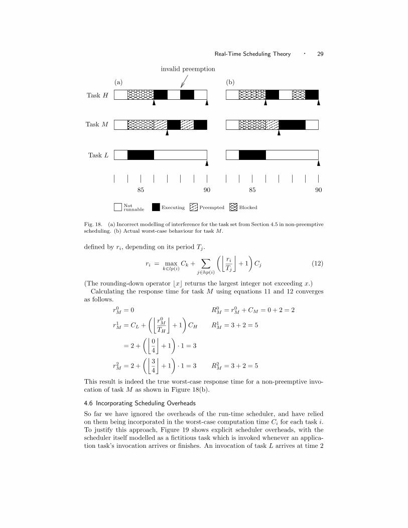
Unfortunately, however, equation 10 can be too naıve. Its interference term isunnecessarily pessimistic because it assumes that an invocation of task i can bepreempted once started [Burns and Wellings 1996b, App. I]. The scenario shownin Figure 18(a) illustrates why the above calculation using equation 10 gave aresponse time of 6 for task M . In practice, though, the context switch at time 88will never occur—once an invocation of task M has started executing, the newly-arrived invocation of task H cannot preempt it.

Therefore, a less pessimistic response time calculation can be used for non-preemptive scheduling [Burns and Wellings 1996b, App. I]. This is done in twoparts. Firstly, task i’s response time Ri in the non-preemptive case is defined to beits computation time Ci plus its release time ri, i.e., the delay between its arrivaland the time it can actually start executing.

Ri = ri + Ci (11)

Secondly, task i’s release time is defined as its worst-case ‘blocking’ from a non-preemptible lower-priority invocation of some task k, plus the interference due toarrivals of each higher-priority task j. To be safely pessimistic in the latter case,it is assumed that each such task j will arrive at least once before the invocationof task i can get started, plus there may be more arrivals of task j in the interval


��

��

��

��

��

��

��

��

��

��

��

��

� � � � � �

��

��

��

��

��

��

��


Task M

Task H

Task L

Blocked

85 90

(a)

invalid preemption

85 90

(b)

Fig. 18. (a) Incorrect modelling of interference for the task set from Section 4.5 in non-preemptivescheduling. (b) Actual worst-case behaviour for task M .

defined by ri, depending on its period Tj .

ri = maxk∈lp(i)

Ck +∑

j∈hp(i)

(⌊ri

Tj

⌋+ 1

)Cj (12)

(The rounding-down operator bxc returns the largest integer not exceeding x.)Calculating the response time for task M using equations 11 and 12 converges

as follows.

r0M = 0 R0

M = r0M + CM = 0 + 2 = 2

r1M = CL +

(⌊r0M

TH

⌋+ 1

)CH

= 2 +(⌊

04

⌋+ 1

)· 1 = 3

R1M = 3 + 2 = 5

r2M = 2 +

(⌊34

⌋+ 1

)· 1 = 3 R2

M = 3 + 2 = 5

This result is indeed the true worst-case response time for a non-preemptive invo-cation of task M as shown in Figure 18(b).

4.6 Incorporating Scheduling Overheads

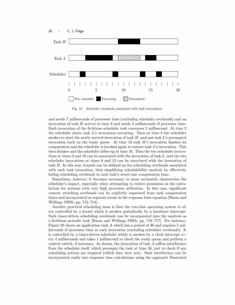
So far we have ignored the overheads of the run-time scheduler, and have reliedon them being incorporated in the worst-case computation time Ci for each task i.To justify this approach, Figure 19 shows explicit scheduler overheads, with thescheduler itself modelled as a fictitious task which is invoked whenever an applica-tion task’s invocation arrives or finishes. An invocation of task L arrives at time 2

30 · C. J. Fidge

��

��

��

0 5 10 15 20


Task H

Task L

Scheduler

Fig. 19. Scheduler overheads associated with task invocations.

and needs 7 milliseconds of processor time (excluding scheduler overheads) and aninvocation of task H arrives at time 8 and needs 4 milliseconds of processor time.Each invocation of the fictitious scheduler task consumes 1 millisecond. At time 2the scheduler starts task L’s invocation executing. Then at time 8 the schedulerawakes to start the newly-arrived invocation of task H, and put task L’s preemptedinvocation back on the ready queue. At time 13 task H’s invocation finishes itscomputation and the scheduler is invoked again to restore task L’s invocation. Thisthen finishes and the scheduler tidies-up at time 16. Thus the two scheduler invoca-tions at times 2 and 16 can be associated with the invocation of task L, and the twoscheduler invocations at times 8 and 13 can be associated with the invocation oftask H. In this way, bounds can be defined on the scheduling overheads associatedwith each task invocation, thus simplifying schedulability analysis by effectivelyhiding scheduling overheads in each task’s worst-case computation time.

Sometimes, however, it becomes necessary to more accurately characterise thescheduler’s impact, especially when attempting to reduce pessimism in the calcu-lations for systems with very high processor utilisation. In this case, significantcontext switching overheads can be explicitly separated from task computationtimes and incorporated as separate terms in the response time equation [Burns andWellings 1995b, pp. 713–714].

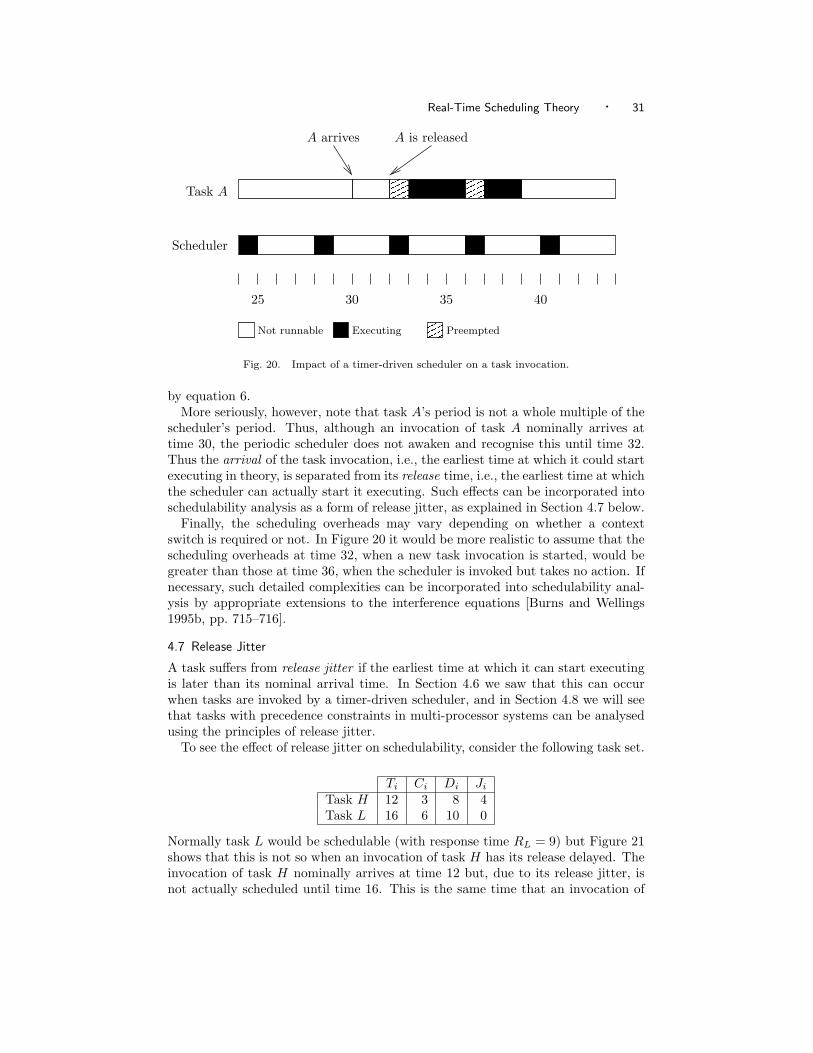
Another practical scheduling issue is that the run-time operating system is of-ten controlled by a kernel which is awoken periodically by a hardware interrupt.Such timer-driven scheduling overheads can be incorporated into the analysis asa fictitious periodic task [Burns and Wellings 1995b, pp. 716–717]. For instance,Figure 20 shows an application task A which has a period of 30 and requires 5 mil-liseconds of processor time at each invocation (excluding scheduler overheads). Itis controlled by a timer-driven scheduler which is awoken by a clock interrupt ev-ery 4 milliseconds and takes 1 millisecond to check the ready queue and perform acontext switch, if necessary. As shown, the invocation of task A suffers interferencefrom the scheduler itself, which preempts the task at time 36, just to check if anyscheduling actions are required (which they were not). Such interference can beincorporated easily into response time calculations using the approach illustrated


��

��

�� 3525 30 40

PreemptedNot runnable

Task A

Scheduler

Executing

A arrives A is released

Fig. 20. Impact of a timer-driven scheduler on a task invocation.

by equation 6.More seriously, however, note that task A’s period is not a whole multiple of the

scheduler’s period. Thus, although an invocation of task A nominally arrives attime 30, the periodic scheduler does not awaken and recognise this until time 32.Thus the arrival of the task invocation, i.e., the earliest time at which it could startexecuting in theory, is separated from its release time, i.e., the earliest time at whichthe scheduler can actually start it executing. Such effects can be incorporated intoschedulability analysis as a form of release jitter, as explained in Section 4.7 below.

Finally, the scheduling overheads may vary depending on whether a contextswitch is required or not. In Figure 20 it would be more realistic to assume that thescheduling overheads at time 32, when a new task invocation is started, would begreater than those at time 36, when the scheduler is invoked but takes no action. Ifnecessary, such detailed complexities can be incorporated into schedulability anal-ysis by appropriate extensions to the interference equations [Burns and Wellings1995b, pp. 715–716].

4.7 Release Jitter

A task suffers from release jitter if the earliest time at which it can start executingis later than its nominal arrival time. In Section 4.6 we saw that this can occurwhen tasks are invoked by a timer-driven scheduler, and in Section 4.8 we will seethat tasks with precedence constraints in multi-processor systems can be analysedusing the principles of release jitter.

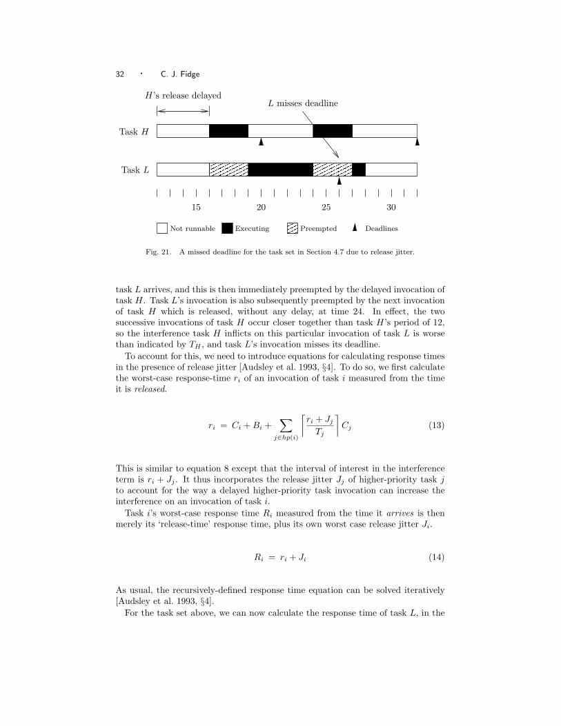
To see the effect of release jitter on schedulability, consider the following task set.

Ti Ci Di Ji

Task H 12 3 8 4Task L 16 6 10 0

Normally task L would be schedulable (with response time RL = 9) but Figure 21shows that this is not so when an invocation of task H has its release delayed. Theinvocation of task H nominally arrives at time 12 but, due to its release jitter, isnot actually scheduled until time 16. This is the same time that an invocation of

32 · C. J. Fidge

��

��

��

��

��

��

30252015

Task L

Deadlines

Task H

Not runnable

L misses deadlineH’s release delayed

PreemptedExecuting

Fig. 21. A missed deadline for the task set in Section 4.7 due to release jitter.

task L arrives, and this is then immediately preempted by the delayed invocation oftask H. Task L’s invocation is also subsequently preempted by the next invocationof task H which is released, without any delay, at time 24. In effect, the twosuccessive invocations of task H occur closer together than task H’s period of 12,so the interference task H inflicts on this particular invocation of task L is worsethan indicated by TH , and task L’s invocation misses its deadline.

To account for this, we need to introduce equations for calculating response timesin the presence of release jitter [Audsley et al. 1993, §4]. To do so, we first calculatethe worst-case response-time ri of an invocation of task i measured from the timeit is released.

ri = Ci + Bi +∑

j∈hp(i)

⌈ri + Jj

Tj

⌉Cj (13)

This is similar to equation 8 except that the interval of interest in the interferenceterm is ri + Jj . It thus incorporates the release jitter Jj of higher-priority task jto account for the way a delayed higher-priority task invocation can increase theinterference on an invocation of task i.

Task i’s worst-case response time Ri measured from the time it arrives is thenmerely its ‘release-time’ response time, plus its own worst case release jitter Ji.

Ri = ri + Ji (14)

As usual, the recursively-defined response time equation can be solved iteratively[Audsley et al. 1993, §4].

For the task set above, we can now calculate the response time of task L, in the


light of task H’s release jitter, using equations 13 and 14 as follows.

r0L = 0

r1L = CL + BL +

⌈r0L + JH

TH

⌉CH = 6 + 0 +

⌈0 + 412

⌉· 3 = 9

r2L = 6 +

⌈9 + 412

⌉· 3 = 12

r3L = 6 +

⌈12 + 4

12

⌉· 3 = 12

RL = r3L + JL = 12 + 0 = 12

This calculated worst-case response time is exactly the result shown in Figure 21.

4.8 Multi-Processor Scheduling Theory

Applying scheduling theory to multi-processor transactions means that inter-proc-essor communication overheads and precedence constraints must be considered dur-ing the analysis.

In the analysis model, the effect of asynchronous message-passing overheads canbe handled by treating the network as a fictitious processor and the messages asfictitious tasks residing on this processor [Richard et al. 2001]. (Section 4.8.1 belowillustrates this.) Alternatively, the effect of blocking forms of communication, suchas accessing a shared data bus, can be modelled by adding a fictitious high-priority‘network task’ to ‘block’ (preempt) tasks that must access the bus [Briand and Roy1999, pp. 175–176].

Precedence constraints between tasks on different machines can be handled eitherby performing ‘whole system’ schedulability analysis (Section 4.8.1) or, if offsets areused to implement precedence constraints, by offset-based analysis (Section 4.8.2).

4.8.1 Holistic Analysis. It is tempting to think that schedulability analysis for amulti-processor system could be achieved merely by performing a separate analysisfor each processor. However, the cross-processor impact of precedence constraintsmeans that the problem is not partitionable in general [Grigg and Audsley 1999,§3.2]. Therefore, ‘holistic’ schedulability analysis aims to extend uni-processor anal-ysis concepts for a whole multi-processor system [Tindell and Clark 1994].

Section 4.7 explained how tasks whose release is delayed can be analysed. Inholistic schedulability analysis this capability is used to model the effects of prece-dence constraints. In Figure 9, for instance, high-priority transaction H can bemodelled by assuming the three individual task invocations arrive simultaneouslyat time 0, but that task Hproc’s invocation suffers from release jitter while waitingfor its message from task Hin’s invocation, and similarly for the invocation of taskHout while waiting for task Hproc’s invocation to finish. Thus the first task in atransaction is modelled as periodic, and the subsequent ones are treated as periodicwith release jitter [Falardeau 1994, p. 46].

The xth approximation to task i’s release (starting time) jitter is calculated interms of its predecessor’s response times as follows [Richard et al. 2001]. Let pre(i)be the set of tasks that belong to the same transaction as task i and occur before

34 · C. J. Fidge

��

��

��

��

��

��

��

151050

Processor B

Processor A

Hi-pri task executing Lo-pri task executing Messages

RL

HB LB

HA LA HA

HB HB HB LB

message LM

Fig. 22. Example of multi-processor transaction scheduling for the task set in Section 4.8.1.

task i in the precedence ordering.

Jxi = max

j∈pre(i)Rx

j (15)

In other words, the earliest time at which task i’s invocation can start executing isthe latest time at which one of its predecessors can finish.

The xth approximation of task i’s response time relative to its release time isthen calculated via equation 13.

rxi = Ci + Bi +

∑

j∈hp(i)

⌈rx−1i + Jx−1

j

Tj

⌉Cj (16)

As usual, we let r0i = 0. In the case of a multi-processor system, set hp(i) means

those tasks with higher priority than task i that reside on the same processor as i.Then the xth approximation of task i’s response time relative to its arrival is

defined as follows.

Rxi = rx

i + Jxi (17)

For example, consider the following multi-processor task set, illustrated in Fig-ure 22. (For simplicity we have assumed that there is no intra-processor blocking,although this is added easily.)

Ti Ci Di pre(i)Task HA 8 3 4 –Task LA 16 4 8 –Task LM – 1 – LA

Task HB 4 2 3 –Task LB 16 3 16 LM

There are two processors, A and B. A high-priority task HA resides on proces-sor A and another (unrelated) high-priority task HB resides on processor B. A


low-priority transaction L consists of two tasks, LA and LB , which reside on pro-cessors A and B, respectively. A precedence constraint requires that invocationsof task LB always occur after the corresponding invocation of task LA. This isimplemented by sending a message LM from the first task to the second. In theworst case, each such message takes 1 millisecond to transmit. To account forthis overhead, message LM is represented in the task set as a fictitious task. Thistask resides on its own imaginary processor and fits into transaction L’s precedenceordering between tasks LA and LB . (Since message-passing ‘task’ LM has no com-petition for its ‘processor’ we have not bothered to specify its deadline or period.However, these features can be incorporated if inter-processor communication is viatime-slots on a shared data bus [Tindell and Clark 1994, §3].)

The high-priority tasks’ response times in this example are trivial, using equa-tion 5, because they suffer from no blocking or interference.

RHA = CHA = 3

RHB = CHB = 2

To analyse transaction L, holistic analysis requires that we work our way forwardalong its precedence ordering [Burns and Wellings 1996a, p. 49]. The response timeanalysis for the first task is standard, using equation 7.

R0LA

= 0

R1LA

= CLA+

⌈R0

LA

THA

⌉CHA

= 4 +⌈

08

⌉· 3 = 4

R2LA

= 4 +⌈

48

⌉· 3 = 7

R3LA

= 4 +⌈

78

⌉· 3 = 7

Also, this task does not suffer from release jitter, so JLA= 0.

The fictitious communications task LM resides on its own imaginary processorand thus suffers from no blocking or interference. However, as per equation 15, itdoes have release jitter due to its dependence on task LA.

J0LM

= 0

J1LM

= R1LA

= 4

J2LM

= R2LA

= 7...

Its response time, calculated using equations 16 and 17, is therefore affected only bythis jitter and its own imaginary computation time (message propagation delay).

r0LM

= 0 R0LM

= r0LM

+ J0LM

= 0

r1LM

= CLM = 1 R1LM

= r1LM

+ J1LM

= 1 + 4 = 5

r2LM

= 1 R2LM

= 1 + 7 = 8

r3LM

= 1 R3LM

= 1 + 7 = 8

36 · C. J. Fidge

The final task in transaction L’s precedence ordering suffers release jitter whilewaiting for message LM to arrive.

J0LB

= 0

J1LB

= R1LM

= 5

J2LB

= R2LM

= 8...

It also suffers interference from the higher-priority task on its processor. Task HB

has no release jitter, so JHB= 0. Task LB ’s response time is then calculated using

equations 16 and 17.

r0LB

= 0 R0LB

= r0LB

+ J0LB

= 0

r1LB

= CLB +⌈

r0LB

+ J0HB

THB

⌉CHB

= 3 +⌈

0 + 04

⌉· 2 = 3

R1LB

= r1LB

+ J1LB

= 3 + 5 = 8

r2LB

= 3 +⌈

3 + 04

⌉· 2 = 5 R2

LB= 5 + 8 = 13

r3LB

= 3 +⌈

5 + 04

⌉· 2 = 7 R3

LB= 7 + 8 = 15

r4LB

= 3 +⌈

7 + 04

⌉· 2 = 7 R4

LB= 7 + 8 = 15

This gives us the total worst-case response time for transaction L, as confirmed bythe instance shown in Figure 22.

4.8.2 Offset-Based Analysis. In Section 3.8 we noted that precedence-constrainedtasks can be implemented using offsets. The offsets are chosen so that the (n+1)thtask in the precedence ordering of a transaction is given an offset at least as greatas the worst-case response time of the nth task [Bate and Burns 1999]. A signifi-cant advantage of this is that schedulability analysis then becomes partitionable—uniprocessor analysis techniques can be applied independently to each machine[Falardeau 1994, p. 48].

However, analysing task sets that use offsets differs from the situation wheretasks experience release jitter (Section 4.7). A task’s worst-case release jitter Ji isan upper bound—an invocation of task i may have its release delayed by up to thisduration. However, a task’s offset Oi is a lower bound—every invocation of task iwill have its release delayed by at least this duration.

In the case where each task i has an offset Oi, the schedulability test for task iis simply modified as follows [Burns and Wellings 1996a, p. 49].

Oi + Ri 6 Di (18)

Importantly, the calculation for response time Ri uses equation 8 and thus dependsonly on tasks that reside on the same processor as task i. Unlike the holisticapproach (Section 4.8.1), an offset-based implementation allows each processor to


be analysed for schedulability separately from other processors. With offsets, thesystem is thus structured in a way that simplifies schedulability analysis. Also, useof offsets can reduce overall task jitter.

However, although safe, test 18 can be overly pessimistic. For instance, considerthe following (uniprocessor) task set.

Ti Ci Di Oi

Task H 4 2 3 0Task L 4 2 3 2

Clearly this task set is schedulable. The first invocation of task H executes betweentimes 0 to 2, the second between times 4 and 6, and so on, whereas the first invoca-tion of task L executes between times 2 and 4, the second between times 6 and 8,etc. However, applying equation 8 to task L gives a response time of 4, exceedingits deadline, so the task is deemed unschedulable by test 18. (Keep in mind thattask L’s deadline is measured relative to its arrival, so the absolute deadline for itsfirst invocation is 5, the second is 9, etc.) The problem is that the standard re-sponse time analysis defined by equation 8 fails to account for the different phasingof the two tasks, which in this case eliminated potential interference.

Developing less pessimistic schedulability tests for offset-based implementationsis still a research topic. It can be approached either by devising modifications tothe response time equation to define interference and blocking with respect to theperiods and offsets of other tasks [Bate and Burns 1999]. Alternatively, similarresults can be achieved using the standard response time equation by devising animaginary task set for analysis which groups tasks by their periods and offsets [Bate1999].

5. OTHER ISSUES

In this section we discuss two concerns for the practical application of schedulingtheory.

5.1 Determining Worst-Case Execution Times

Scheduling theory assumes that the programmer can supply accurate estimates forthe worst-case computation time Ci for each task i and the worst-case blocking timeBi due to tasks of lower priority. Both of these figures depend on the execution timeof (sequential) code fragments from the task bodies. (With respect to Figure 3, thecomputation time for an invocation of this task is determined by how long it takesto perform one complete iteration of the loop, excluding any periods of suspension.)However, analysing program code for its worst-case execution time is a challengingproblem in its own right. Moreover, it is important for the results to be as accurateas possible. Pessimistic estimates will mean that the schedulability tests may failschedulable task sets, leading to unnecessary optimisation of the program. Evenworse, overly optimistic estimates may mean that the tests pass unschedulable tasksets, leading to missed deadlines at run time.

The most obvious way to determine the worst-case execution time for a task invo-cation is to simply execute the task code and measure how long it takes. However,this relies on the test successfully reproducing the worst-case behaviour of the task.Furthermore, such testing can be difficult for embedded control programs because

38 · C. J. Fidge

they must be executed in an appropriate run-time environment, which may requireconstruction of a suitable test harness.

Therefore, worst-case execution time prediction has focussed on syntactic anal-ysis of program code. Initially this was done for high-level language programs bydefining a ‘cost function’ for each language construct and using it to sum the totalexecution-time cost associated with all control-flow paths through a task [Shaw1989] [Puschner and Koza 1989]. This proved difficult to do accurately, however,without detailed knowledge of the compiler’s assembler code generation strategyand optimisations.

Given the difficulties of analysing high-level language programs, recent researchhas concentrated on analysis of compiled machine code. However, even this hasproven difficult. RISC processors are popular for programming real-time systemsbecause of their high processing speeds [Williams 1991]. However, the very fea-tures they use to achieve high performance, such as instruction pipelining and datacaching, introduce nondeterminism into the execution time of the code, and thusthwart attempts to accurately predict worst-case execution times. Therefore, muchresearch has gone into explicitly allowing for such features in machine code analysis[Healy et al. 1995] [Lim et al. 1995] [Theiling et al. 2000] [Hur et al. 1995].

Furthermore, in both high and assembler-level timing prediction, a significantproblem is that many syntactically-valid control-flow paths through program codeare semantically ‘dead’ because they can never be followed at run time. Includingsuch paths in execution time analysis may unnecessarily increase the pessimism ofthe estimate. Therefore, considerable effort has gone into algorithms [Park 1993][Altenbernd 1996] [Ermedahl and Gustafsson 1997] [Lundqvist and Stenstrom 1999]and semantic definitions [Chapman et al. 1996] [Hayes et al. 2001] for identifyingand excluding such dead paths.

5.2 Programming Guidelines

We have seen that scheduling theory assumes a simple ‘computational model’ ofthe task set being analysed. It is therefore important that the actual system isprogrammed in a way compatible with this model. The most important advance inthis direction was the design of the Ada 95 programming language. Its revision ofthe original Ada 83 language specifically took recent progress in scheduling theoryinto account [Stoyenko and Baker 1994]. The resulting language therefore offers nu-merous constructs customised for programming multi-tasking, real-time programsin a way amenable to analysis using scheduling theory. In particular, Ada 95 fea-tures: ‘delay until’ statements for programming periodic tasks; ‘protected objects’for mutually-exclusive access to shared resources; interrupt handlers implementedas (very) high-priority protected procedures; well-defined execution time overheadsfor all language constructs; and default implementations of fixed-priority, preemp-tive task scheduling and priority ceiling locking [Taft and Duff 1997].

However, the Ada language is also very rich and contains many features whosetiming behaviour are hard to reason about. Therefore, an easily-analysable subsetof the language, known as the ‘Ravenscar Profile’ [Burns et al. 1998] is currentlybeing standardised.

Also, although Ada 95 provides strong support for uni-processor schedulabilityanalysis, its support for multi-processor (distributed) real-time systems is not aswell developed [Burns and Wellings 1995a, Ch. 14] and is still the subject of research


[Garcıa and Harbour 2001].Ada 95 remains the best high-level language for programming analysable real-

time systems. Attempts are currently underway to develop analysable versions ofother programming languages, by borrowing concepts from Ada 95 [Brosgol andDobbing 2001], but this work is still in its infancy.

6. APPLYING SCHEDULING THEORY IN PRACTICE

The examples above have shown that the calculations needed to assess schedulabil-ity are simple but tedious. Not surprisingly, therefore, there have been numeroustools developed to perform the necessary arithmetic [Briand and Roy 1999, App. D].For instance, the MetaH programming environment performs basic workload cal-culations using equation 3 [Honeywell Technology Center 1998]. While they savesome effort, such tools do not necessarily give the programmer any insight into thedynamic behaviour of the task set. This can be achieved by simulation tools whichdisplay (worst-case) timelines for a given task set [Audsley et al. 1994] [de Beer andFidge 2000].

We have also seen that scheduling theory has been thoroughly explored in theacademic literature and has progressed dramatically in recent years. However,the extent of its application in practice is harder to judge. For instance, avionicsapplications are often cited in the literature to motivate scheduling principles [Griggand Audsley 1999] [Briand and Roy 1999], but the examples there are relativelysimple, generalised case studies [Locke et al. 1990].

A more realistic application of scheduling theory was to the Olympus satellite’sAttitude and Orbital Control System [Burns and Wellings 1995b]. The system was(re)engineered using fixed-priority preemptive scheduling, with deadline-monotonicpriority allocation, and programmed in Ada. Worst-case computation times werepredicted using an analysis tool integrated into the front-end of the Ada compiler. Itwas found that context switching times were significant in this system, so a variantof the response time equations was defined that made these overheads explicit. Thetask set also featured offsets, jitter and variable computation times that needed tobe accounted for in order to produce acceptably accurate results. It was concludedthat although scheduling theory provides ‘a sound theoretical understanding of howto engineer real-time systems’, in a complex application the schedulability equationsmust be customised to match the peculiarities of the particular system [Burns andWellings 1995b].

In the avionics field, a detailed study was undertaken of how basic processor util-isation analysis could be applied to the Mission Computer Software for Canada’sCF-188 fighter aircraft [Falardeau 1994]. The hardware architecture consists oftwo Mission Computers (providing redundancy for fault tolerance) connected bypairs of data buses [Falardeau 1994, §4.1]. Each Mission Computer comprises sev-eral processors, most notably a general purpose Central Processing Unit and adedicated Input/Output Processor. The software architecture of the OperationalFlight Program that resides on each of the Mission Computers is complex. Froma scheduling viewpoint it consists of two types of transactions (confusingly called‘task rates’ in the CF-188 documentation) [Falardeau 1994, §4.3.2]. Firstly, routinesystem functions are programmed as periodic transactions, with a rate monotonicpriority assignment. A clock interrupt-driven kernel is used to schedule periodictransactions. Each such transaction consists of an input task, followed by a pro-

40 · C. J. Fidge

cessing task, and then an output task. The input and output tasks reside on theInput/Output Processor, and the processing task on the Central Processing Unit.The CPU initiates tasks on the IOP by sending queued (asynchronous) ‘I/O request’messages over a bus, whereas the IOP uses an interrupt to signal the completion ofan I/O task to the CPU. Secondly, sporadic actions which must respond quickly toexternal stimuli are implemented as high-priority interrupt-triggered transactionswhich preempt the currently executing transaction.

To analyse this complex system, extensive tables were drawn up to documentthe characteristics of transactions such as the precedence ordering of tasks, theirperiods, deadlines, priorities, worst-case computation times, release jitter charac-teristics, use of shared resources, and so on [Falardeau 1994, §4.4.2]. Sporadictransactions were modelled as periodic ones using their minimum interarrival rateas their period [Falardeau 1994, p. 75]. Overheads associated with the run-timekernel were explicitly considered [Falardeau 1994, p. 77]. Two analysis models werethen applied. The first [Falardeau 1994, §4.4.4] attempted to partition the analy-sis by adding delays due to input and output activities into the computation timeassociated with each task and then applying the basic processor utilisation test(Section 4.1). However, the complex pattern of communication in the system madedefining these delays accurately very difficult. The second approach [Falardeau1994, §4.4.5] used a simple distributed system perspective [Burns and Wellings1996a, p. 49] and attempted to determine the worst-case response times for eachtransaction by following the chain of precedence constraints and summing the taskcomputation times and message propagation delays encountered. Most of the indi-vidual tasks comprising the transactions in the system suffered from considerablerelease jitter due to their precedence constraints. These values were felt to be dif-ficult to calculate, so it was suggested that an offset-based model (Section 4.8.2)would be easier to analyse. Overall, it was concluded that neither approach seemedentirely satisfactory. It is therefore now interesting to ask whether a holistic anal-ysis (Section 4.8.1), which was not available when this study was done, would haveproved more successful.

Finally, apart from these technical challenges, a further practical issue for real-time programmers wanting to apply scheduling theory is that safety certificationstandards for such systems [RTCA, Inc. 1992] have yet to embrace modern multi-tasking programming principles, and therefore impose requirements that restrictthe use of such technology [Burns and Wellings 1996b].

7. CONCLUSIONS

We have seen that real-time scheduling theory has now matured into a powerfuland practical concept. It provides programmers with a predictive theory for as-sessing the capabilities of a multi-tasking system design before its construction iscompleted, and for identifying problems in existing systems. It is thus one aspectof ‘software engineering’ that genuinely has the characteristics of a true engineeringdiscipline.

ACKNOWLEDGMENTS

I wish to thank David Tombs and Antonio Cerone for helping with Section 6,and Robert Colvin for reviewing a draft of this paper. This work was funded by


the Air Operations Division of the Defence Science and Technology Organisation.Particular thanks are due to Drs Zahid Qureshi, Paul Johnson and Thong Nguyen.

REFERENCES

Altenbernd, P. 1996. On the false path problem in hard real-time programs. In Proc. 8thEuromicro Workshop on Real-Time Systems (WRTS) (1996), pp. 102–107.

Audsley, N., Burns, A., Richardson, M., Tindell, K., and Wellings, A. 1993. Apply-ing new scheduling theory to static priority pre-emptive scheduling. Software EngineeringJournal 8, 5 (Sept.), 284–292.

Audsley, N. C., Burns, A., Davis, R. I., Tindell, K. W., and Wellings, A. J. 1995.Fixed priority pre-emptive scheduling: An historical perspective. Real-Time Systems 8,173–198.

Audsley, N. C., Burns, A., Richardson, M. F., and Wellings, A. J. 1992. Deadlinemonotonic scheduling theory. In Proceedings 18th IFAC/IFIP Workshop on Real-TimeProgramming (WRTP’92) (June 1992).

Audsley, N. C., Burns, A., Richardson, M. F., and Wellings, A. J. 1994. STRESS:A simulator for hard real-time systems. Software—Practice & Experience 24, 6 (June),543–564.

Baker, T. P. 1990. A stack-based resource allocation policy for realtime processes. In Proc.Real-Time Systems Symposium (Dec. 1990), pp. 191–200. IEEE Computer Society Press.

Baker, T. P. 1991. Stack-based scheduling of real-time processes. Real Time Systems 3, 1(March), 67–99.

Baker, T. P. and Shaw, A. 1989. The cyclic executive model and Ada. Journal of Real-Time Systems 1, 1 (June), 7–26.

Bate, I. 1999. Scheduling and Timing Analysis for Safety Critical Real-Time Systems. Ph.D. thesis, Department of Computer Science, The University of York.

Bate, I. and Burns, A. 1999. A framework for scheduling and schedulability analysis forsafety-critical embedded control systems. Draft, Department of Computer Science, TheUniversity of York.

Blazquez, V., Redondo, L., and Freniche, J. L. 1992. Experiences with delay until foravionics computers. Ada Letters XII, 1 (Jan/Feb), 65–72.

Briand, L. P. and Roy, D. M. 1999. Meeting Deadlines in Hard Real-Time Systems: TheRate Monotonic Approach. IEEE Computer Society.

Brosgol, B. and Dobbing, B. 2001. Can Java meet its real-time deadlines? InD. Craeynest and A. Stroheimer Eds., Reliable Software Technologies (Proceedings ofAda-Europe 2001), Volume 2043 of Lecture Notes in Computer Science (2001), pp. 68–87.Springer-Verlag.

Burns, A., Dobbing, B., and Romanski, G. 1998. The Ravenscar tasking profile for highintegrity real-time programs. In L. Asplund Ed., Reliable Software Technologies—Ada-Europe ’98 , Volume 1411 of Lecture Notes in Computer Science (1998), pp. 263–275.Springer-Verlag.

Burns, A. and Wellings, A. 1996a. Advanced fixed priority scheduling. In M. JosephEd., Real-Time Systems: Specification, Verification and Analysis, Chapter 3, pp. 32–65.Springer-Verlag.

Burns, A. and Wellings, A. J. 1990. Real-Time Systems and Their Programming Lan-guages. Addison-Wesley.

Burns, A. and Wellings, A. J. 1995a. Concurrency in Ada. Cambridge University Press.

Burns, A. and Wellings, A. J. 1995b. Engineering a hard real-time system: From theoryto practice. Software–Practice & Experience 25, 7 (July), 705–726.

Burns, A. and Wellings, A. J. 1996b. Simple Ada 95 tasking models for high integrityapplications. Department of Computer Science, University of York.

Buttazzo, G. C. 1997. Hard Real-Time Computing Systems: Predictable Scheduling Al-gorithms and Applications. Kluwer.

42 · C. J. Fidge

Chapman, R., Burns, A., and Wellings, A. 1996. Combining static worst-case timinganalysis and program proof. Real-Time Systems 11, 145–171.

Chen, M.-I. and Lin, K.-J. 1990. Dynamic priority ceilings: A concurrency control protocolfor real-time systems. Journal of Real-Time Systems 2, 4 (Nov.), 325–346.

de Beer, A. and Fidge, C. J. 2000. A simple multi-tasking simulator. Technical Report00-28 (Aug.), Software Verification Reseach Centre, The University of Queensland.

Embedded Systems Programming. 2001. Buyer’s guide 2002. Special Issue, Volume 14,Number 9.

Ermedahl, A. and Gustafsson, J. 1997. Deriving annotations for tight calculation of exe-cution time. In C. Lengauer, M. Griebel, and S. Gorlatch Eds., Euro-Par’97: ParallelProcessing, Volume 1300 of Lecture Notes in Computer Science (1997), pp. 1298–1307.Springer-Verlag.

Falardeau, J. D. G. 1994. Schedulability analysis in rate monotonic based systems withapplication to the CF-188. Master’s thesis, Department of Electrical and Computer Engi-neering, Royal Military College of Canada.

Fidge, C. J. 1998. Real-time schedulability tests for preemptive multitasking. Real-TimeSystems 14, 1 (Jan.), 61–93.

Fidge, C. J., Hayes, I. J., and Watson, G. 1999. The deadline command. IEEProceedings—Software 146, 2 (April), 104–111.

Garcıa, J. J. G. and Harbour, M. G. 2001. Towards a real-time distributed systemsannex in Ada. Ada Letters XXI, 1 (March), 62–66.

Giering III, E. and Baker, T. 1994. A tool for deterministic scheduling of real-time pro-grams implemented as periodic ada tasks. ACM Ada Letters XIV, 54–73.

Gomaa, H. 1993. Software Design Methods for Concurrent and Real-Time Systems.Addison-Wesley.

Grigg, A. and Audsley, N. C. 1999. Towards a scheduling and timing analysis solutionfor integrated modular avionics systems. Microprocessors and Microsystems 22, 423–431.

Hayes, I. J., Fidge, C. J., and Lermer, K. 2001. Semantic characterisation of deadcontrol-flow paths. IEE Proceedings—Software 148, 6 (Dec.), 175–186.

Healy, C. A., Whalley, D. B., and Harmon, M. G. 1995. Integrating the timing analysisof pipelining and instruction caching. In Proc. 16th IEEE Real-Time Systems Symposium(Dec. 1995), pp. 288–297. IEEE Computer Society Press.

Honeywell Technology Center. 1998. MetaH User’s Manual (1.27 ed.). Honeywell Technol-ogy Center. http://www.htc.honeywell.com/metah/prodinfo.html.

Hur, Y., Bae, Y. H., Lim, S.-S., Rhee, B.-D., Min, S. L., Park, C. Y., Lee, M., Shin, H.,and Kim, C. S. 1995. Worst case timing analysis of RISC processors: R3000/R3010case study. In Proc. 16th IEEE Real-Time Systems Symposium (Dec. 1995), pp. 308–319.IEEE Computer Society Press.

Jones, M. B., Barrera III, J. S., Forin, A., Leach, P. J., Rosu, D., and Rosu, M.-C.1996. An overview of the Rialto real-time architecture. In Proc. Seventh ACM SIGOPSEuropean Workshop (Sept. 1996).

Joseph, M. and Pandya, P. 1986. Finding response times in a real-time system. TheComputer Journal 29, 5, 390–395.

Kalinsky, D. 2001. Context switch. Embedded Systems Programming 14, 2 (Feb.), 94–105.

Kristenssen, L. M., Billington, J., and Qureshi, Z. H. 2001. Modelling military air-borne mission systems for functional analysis. In Proceedings of the 20th Digital AvionicsSystems Conference (DASC) (Oct. 2001).

Kurki-Suonio, R. 1994. Real time: Further misconceptions (or half-truths). IEEE Com-puter , 71–76.

Lehoczky, J. P., Sha, L., and Ding, Y. 1989. The rate monotonic scheduling algorithm:Exact characterization and average case behavior. In Proc. Real-Time Systems Symposium(1989), pp. 166–171. IEEE Computer Society Press.

Lim, S.-S., Bae, Y. H., Jang, G. T., Rhee, B.-D., Min, S. L., Park, C. Y., Shin, H., Park,K., Moon, S.-M., and Kim, C. S. 1995. An accurate worst case timing analysis forRISC processors. IEEE Transactions on Software Engineering 21, 7 (July), 593–604.


Liu, C. L. and Layland, J. W. 1973. Scheduling algorithms for multiprogramming in ahard real-time environment. Journal of the ACM 20, 1, 46–61.

Locke, C. D. 1992. Software architecture for hard real-time applications: Cyclic executivesvs. fixed priority executives. The Journal of Real-Time Systems 4, 37–53.

Locke, C. D., Vogel, D. R., Lucas, L., and Goodenough, J. B. 1990. Generic avionicssoftware specification. Technical Report CMU/SEI-90-TR-8 (Dec.), Software EngineeringInsititute, Carnegie Mellon University.

Lundqvist, T. and Stenstrom, P. 1999. An integrated path and timing analysis methodbased on cycle-level symbolic execution. Real-Time Systems 17, 2/3 (Nov.), 183–207.

Park, C. Y. 1993. Predicting program execution times by analyzing static and dynamicprogram paths. Real-Time Systems 5, 31–62.

Pilling, M., Burns, A., and Raymond, K. 1990. Formal specifications and proofs ofinheritance protocols for real-time scheduling. Software Engineering Journal 5, 5 (Sept.),263–279.

Puschner, P. and Koza, C. 1989. Calculating the maximum execution time of real-timeprograms. Journal of Real-Time Systems 1, 2 (Sept.), 159–176.

Richard, P., Cottet, F., and Richard, M. 2001. On-line scheduling of real-time dis-tributed computers with complex communication constraints. In Proceedings of the SeventhIEEE International Conference on Engineering of Complex Computer Systems (2001), pp.26–34. IEEE Computer Society.

RTCA, Inc. 1992. Software Considerations in Airborne Systems and Equipment Certifica-tion. RTCA, Inc. Special Committee 167 Document No. RTCA/DO-178B.

Sha, L., Rajkumar, R., and Lehoczky, J. 1990. Priority inheritance protocols: An ap-proach to real-time synchronization. IEEE Trans. Computers 39, 9 (Sept.), 1175–1185.

Shaw, A. C. 1989. Reasoning about time in higher-level language software. IEEE Trans-actions on Software Engineering 15, 7 (July), 875–889.

Sprunt, B., Sha, L., and Lehoczky, J. 1989. Aperiodic task scheduling for hard real-timesystems. Journal of Real-Time Systems 1, 1 (June), 27–60.

Stankovic, J. A. 1988. Misconceptions about real-time computing. IEEE Computer 21, 10(Oct.), 10–19.

Stankovic, J. A. and Ramamritham, K. 1990. Editorial: What is predictability for real-time systems. Journal of Real-Time Systems 2, 4 (Nov.), 247–254.

Stewart, D. B. 2001. Beginner’s corner: Real time. Embedded Systems Program-ming 14, 12 (Nov.), 87–88.

Stoyenko, A. D. and Baker, T. P. 1994. Real-time schedulability-analyzable mechanismsin Ada 9X. Proceedings of the IEEE 82, 1 (Jan.), 95–107.

Taft, S. T. and Duff, R. A. Eds. 1997. Ada 95 Reference Manual: Language and StandardLibraries, Volume 1246 of Lecture Notes in Computer Science. Springer-Verlag.

Theiling, H., Ferdinand, C., and Wilhelm, R. 2000. Fast and precise WCET predic-tion by separated cache and path analyses. The International Journal of Time-CriticalComputing Systems 18, 2/3 (May), 157–179.

Tindell, K. 2000. Deadline monotonic analysis. Embedded Systems Programming 13, 6(June), 20–38.

Tindell, K., Burns, A., and Wellings, A. J. 1994. An extendible approach for analyzingfixed priority hard real-time tasks. Real-Time Systems 6, 133–151.

Tindell, K. and Clark, J. 1994. Holistic schedulability analysis for distributed hard real-time systems. Euromicro Journal 40, 117–134. Special Issue on Parallel Embedded Real-Time Systems.

Williams, T. 1991. Performance pushes RISC chips into real-time roles. Computer Design,79–86.

Date post:	18-Feb-2019
Category:	Documents
Upload:	phamthuy
View:	227 times
Download:	0 times

SOFTWARE VERIFICATION RESEARCH CENTRE THE UNIVERSITY …10543/svrc_02_19.pdf · SOFTWARE...

Documents