Soil Dynamics Prof. Dr. Deepankar Choudhury Department of Civil Engineering

Indian Institute of Technology, Bombay

Module - 2 Vibration Theory

Lecture - 3 PSDOF system, Types of Vibrations, Free Vibration

Let us start with today’s lecture on soil dynamics. As we had discussed in the previous

lecture, let us look at the slide, for this course on soil dynamics. We are now going

through module two on vibration theory.

(Refer Slide Time: 00:47)

And, as a recap of what we have learnt in the previous lecture, like for simple vibrating

system, what we refer as single degree of freedom system SDOF system, with mass

spring and damper, MSD system we call them generally, which looks like this, with free

body diagram like this. And, among this three important components: mass relates to the

kinetic energy, stiffness relates to the potential energy, and the damper relates to the

dissipation or loss of energy. Then, we have seen, what is D’Allembert’s principle.

(Refer Slide Time: 01:26)

And, considering the linear model for all the resistive forces that is spring force, inertia

force, and damper force, we have seen that the linear model for equation of motion

comes down for the single degree of freedom system, like this; mass times acceleration is

our inertia force plus damping coefficient times velocity gives us the damper force or

loss of energy plus stiffness times displacement gives us the stiffness force equals to

externally applied dynamic load.

So, governing equation of motion, for linear model for a single degree of freedom system

is m u double dot plus c u dot plus k u equals to p of t, where u of t is the response or

displacement function with respect to time. And also, we have seen, what are the units

for this common parameters m, k, and c in different systems, like in MLT system, in FLT

system, and in SI unit So, conventionally, we use for our problems the SI units: for mass

as k g, for stiffness as Newton per meter, and for the damper as Newton second per

meter.

(Refer Slide Time: 03:00)

We have also seen in the previous lecture that what are the different types of vibrations?

We can classify vibration into 2 major categories: one is called free vibration in which

the externally applied dynamic load p of t equals to 0, and another one is forced vibration

where the externally applied dynamic load is non-zero.

Again, within each of this vibrations we can sub classify them into 2 categories, like for

free vibration we can sub classify them as undamped free vibration and damped free

vibration; we call undamped free vibration when the damper that is c is not present that

is c equals to 0, and also p of t equals to 0 that we call as undamped free vibration; and

the damped free vibration is when the damper is present that is c is non-zero, then we can

call that as damped free vibration.

Now, coming to forced vibration also, the same two conditions, we can mention that 2

types of vibration: one is undamped forced vibration, when c equals to 0, but p t is non-

zero; another one is damped forced vibration that is when c not equals to 0, and p of t is

not equals to 0. Again, another way to classify the forced vibration we have seen, there

can be two categories: one is called periodic forced vibration, and another is called a

periodic forced vibration. We have seen the examples of periodic forced vibration, like

any externally applied dynamic load when it is applied follows some period means

regular period like any harmonic motion, in that case can be classified as periodic type

forced vibration; and aperiodic when it is not following any period then we call that as

aperiodic forced vibration.

Again, the sub classification within a periodic forced vibration we have seen, one is

called transient type a periodic forced vibration, and the other one we call steady state

type aperiodic forced vibration. Transient, which we call transient? When the time for

which the dynamic load is acting is finite that we call a transient type a period forced

vibration, for example, earthquake load which occurs for a finite duration of time. And,

the steady state type aperiodic forced vibration, when the time for which the dynamic

load is acting on the system is tending to infinity that we classify as steady state a

periodic forced vibration; and as an example we have seen wind load when it is acting on

any structural system that we generally classify as steady state type aperiodic forced

vibration.

(Refer Slide Time: 06:20)

Now, what we have seen in the single degree of freedom system? Whether it is

horizontally vibrating, or whether it is vertically vibrating system, it does not matter the

equation of motion, governing equation of motion remains same; only thing, the

displacement function which we finally obtain from after solving the equation that is the

dynamic component of the displacement. If we want to find out the total displacement

then we need to add the static component of the displacement; that we have seen in the

previous class.

(Refer Slide Time: 06:59)

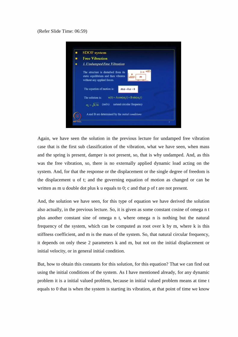
Again, we have seen the solution in the previous lecture for undamped free vibration

case that is the first sub classification of the vibration, what we have seen, when mass

and the spring is present, damper is not present, so, that is why undamped. And, as this

was the free vibration, so, there is no externally applied dynamic load acting on the

system. And, for that the response or the displacement or the single degree of freedom is

the displacement u of t; and the governing equation of motion as changed or can be

written as m u double dot plus k u equals to 0; c and that p of t are not present.

And, the solution we have seen, for this type of equation we have derived the solution

also actually, in the previous lecture. So, it is given as some constant cosine of omega n t

plus another constant sine of omega n t, where omega n is nothing but the natural

frequency of the system, which can be computed as root over k by m, where k is this

stiffness coefficient, and m is the mass of the system. So, that natural circular frequency,

it depends on only these 2 parameters k and m, but not on the initial displacement or

initial velocity, or in general initial condition.

But, how to obtain this constants for this solution, for this equation? That we can find out

using the initial conditions of the system. As I have mentioned already, for any dynamic

problem it is a initial valued problem, because in initial valued problem means at time t

equals to 0 that is when the system is starting its vibration, at that point of time we know

either its displacement or its velocity. So, either u or u dot is known to us at time t equals

to 0. So, that is why these are called initial valued problem.

(Refer Slide Time: 09:31)

And, we have seen how to compute the, this constants A and B, like this constants A

comes out to be initial displacement u not, and the other constants B comes out to be

initial velocity divided by the natural frequency. So, the final solution takes a form like

this that is u of t equals u naught cosine omega n t plus u naught dot by omega n sine

omega n t.

Now, this same solution for the equation of motion, we can express it in the form of

polar coordinate system. So, that we have expressed like this, where c is called amplitude

of motion which can be computed like this, and theta is the phase. And, in this the

natural period can be computed using this expression, and the natural frequency can be

computed using this expression. And, the profile or the response of that u, as it varies

with respect to time can be plotted like this, it is a harmonic function the solution, with

the initial condition as initial velocity here, sorry, and initial displacement here, and

initial velocity. It can be either positive velocity, 0 velocity, or negative velocity,

depending on that the starting graph how the response should be depends on, that you

know already.

(Refer Slide Time: 11:14)

We have also learnt how to find out the natural frequency of any system from its static

deflection. That is if we know the static deflection of any system, we can find out its

natural frequency. How? Let us look at the slide; if any mass is hanging from a spring, in

that case it is static deflection can be expressed by weight divided by the spring constant.

Whereas, the natural frequency f can be expressed by 1 by T, T is the time period which

is expressed by 1 by 2 pie root of k by m, this if we put in terms of w and k and rearrange

them, the final expression comes out to be 1 by 2 pie root over g by delta s t, g is

acceleration due to gravity which is known to us, delta s of t is the nothing but the static

displacement which we have computed while hanging that mass from that spring. So, in

that way we can find out the natural frequency from the static deflection.

(Refer Slide Time: 12:33)

We have also seen that, how to compute the equivalent spring stiffness for springs when

they are connected in parallel like this, or when they are connected in series like this. So,

for springs in parallel, if K 1 and K 2, two spring constant at a distance of x 1 plus x 2.

And, if we want to find out an equivalent spring stiffness at point c, so, that point c is at a

distance of x 1 from this spring k 1, and at a distance of x 2 from spring k 2. Then, the

equivalent spring constant comes out by this expression, which we have derived in the

previous lecture. And, when springs are connected in series like this, the equivalent

spring constant can be expressed by this expression. So, that was our, till last lecture

what we have covered.

Now, let us start today with today’s topic, before I continue with the problems what we

had given in the previous lecture, let me give some more expressions for other different

types of loading, like when there is some earthquake excitation how we can formulate

the equation of motion, let us see for a single degree of freedom system. Let us look at

the page here.

(Refer Slide Time: 14:11)

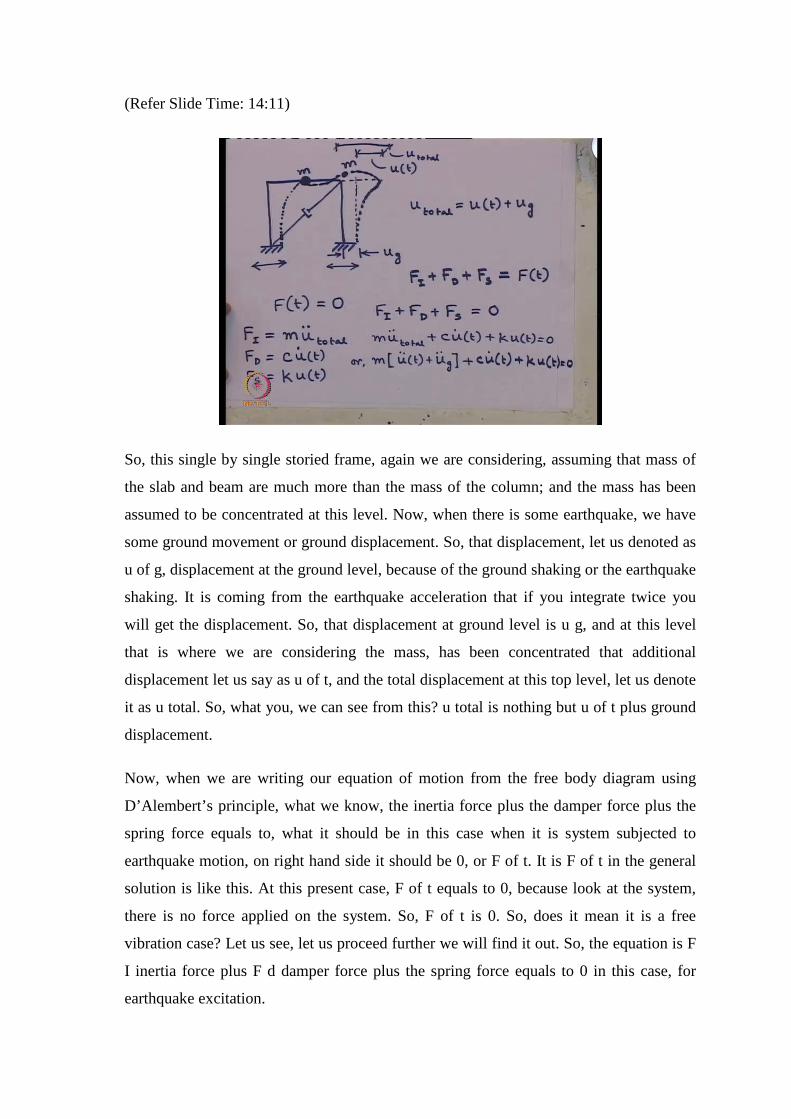
So, this single by single storied frame, again we are considering, assuming that mass of

the slab and beam are much more than the mass of the column; and the mass has been

assumed to be concentrated at this level. Now, when there is some earthquake, we have

some ground movement or ground displacement. So, that displacement, let us denoted as

u of g, displacement at the ground level, because of the ground shaking or the earthquake

shaking. It is coming from the earthquake acceleration that if you integrate twice you

will get the displacement. So, that displacement at ground level is u g, and at this level

that is where we are considering the mass, has been concentrated that additional

displacement let us say as u of t, and the total displacement at this top level, let us denote

it as u total. So, what you, we can see from this? u total is nothing but u of t plus ground

displacement.

Now, when we are writing our equation of motion from the free body diagram using

D’Alembert’s principle, what we know, the inertia force plus the damper force plus the

spring force equals to, what it should be in this case when it is system subjected to

earthquake motion, on right hand side it should be 0, or F of t. It is F of t in the general

solution is like this. At this present case, F of t equals to 0, because look at the system,

there is no force applied on the system. So, F of t is 0. So, does it mean it is a free

vibration case? Let us see, let us proceed further we will find it out. So, the equation is F

I inertia force plus F d damper force plus the spring force equals to 0 in this case, for

earthquake excitation.

Now, how much is our F of I that is inertia force in this case? Inertia is mass times

acceleration; how much is the acceleration? The mass is experiencing in this, mass has

moved a distance of u total. So, acceleration corresponding to u total, will act on this

mass as inertia force. So, F I is nothing but m times u double dot total; and the damper

force, F of d is nothing but c damping constant times the velocity. Now, what we know?

The velocity is the relative velocity between the 2 ns of a damper. So, what is the relative

velocity here, about the 2 ns? It will be u dot of t that is the relative velocity. And, what

is the spring force? That is also the spring constant k times the relative displacement.

What is the relative displacement between this point and this point? That is u of t.

So, if we put this expressions in our D’Alembert’s principle, whatever expression we

have got here, it comes out to be m u double dot total plus c u dot t plus k u of t equals to

0; or, m u double dot t plus u g double dot, look here, the total displacement was u of t

plus u of ground, and that u of ground we can differentiate twice to get the acceleration

at the ground, which was actually our input from the earthquake motion. So, in this case,

it is possible to differentiate. So, that is why we have written like this, plus c u dot t plus

k u t equals to 0.

(Refer Slide Time: 21:10)

So, the equation now I am rearranging, m u double dot t plus c u dot t plus k u of t equals

to, not 0, am getting here minus m u g double dot. Now, look at this parameter, this is

nothing but the force induced to the system because of earthquake. So, that is why it is

not a free vibration problem, but a forced vibration problem, where the force is coming

from this component that is the what is ground acceleration times the mass of the system.

So, this can be written as our conventional p of t.

Now, this u g double dot that is acceleration due to earthquake at ground level can be

function of time, it will be a function of time of course. So, that is why it can be

expressed as p of t. So, our governing equation of motion takes the same form, and now

we know where from this external dynamic load is acting on the system for a system

subjected to earthquake excitation.

(Refer Slide Time: 22:54)

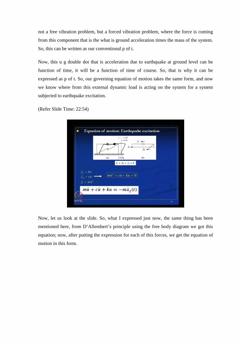
Now, let us look at the slide. So, what I expressed just now, the same thing has been

mentioned here, from D’Allembert’s principle using the free body diagram we got this

equation; now, after putting the expression for each of this forces, we get the equation of

motion in this form.

(Refer Slide Time: 23:17)

So, if we consider a frame subjected to earthquake shaking or earthquake excitation at

ground level with acceleration u g of t double dot, it can be considered as equivalent to a

stationary base subjected to a dynamic load acting on this system at this mass level with

minus m u g double dot t. So, that is our effective dynamic load acting on the system.

(Refer Slide Time: 24:16)

Now, let us move to the solution of the remaining problems, what we had given in the

previous lecture. To start with the fourth problem, we have seen that it says, the bent rod

shown in the figure. So, this is the bent rod has negligible mass. So, this rod is rigid rod,

but we are assuming it is not having any mass, but it is supporting a 5 kg collar at its end.

So, again, as I have mentioned, we always consider in this problems masses are point

mass.

So, this 5 kg collar is concentrated at this end c, what it says, develop the equation of a

motion and determine the natural period of vibration for the system. For the system as

shown here, B is a hinge joint, at joint A there is a link connected to a spring with spring

constant 400 Newton per meter, the arm length of A B is 100 millimeter, and the arm

length of B C is 200 millimeter.

So, let us see, how we can proceed further for this problem. First, we should draw the

free body diagram of this problem, let us do that. So, for a small rotation, the system will

take a shape like this. This is a small rotation theta angle, here also it will make theta

because this is a rigid link. So, at pin joint they will maintain the continuity, and theta is

the small angle of rotation. And, at one instant of time we are considering this is our

direction of motion. So, what are the forces acting on this system now? Here, a mass is

attached. So, this mass will experience a inertia force; a inertia force will act here; in

which direction? Vertically downward, or upward? It should act vertically upward, not

downward. Downward weight will act not the inertia force. Now, why we are not

showing weight? Because, we know from our previous lecture that in case of vertical

mode of vibration, weight is getting balanced with respect to its static displacement and

things like that.

So, after attaining static equilibrium conditions we are proceeding further for this case.

So, inertia force what we are considering here, is acting in this direction, which will try

to put it back in its original position. So, that is why it should act vertically upward

direction. And, at this point there is a spring attached to it which has been compressed, it

will try to come back to its original position. So, the spring force F of S will act in this

direction. Now, this rod is having no mass. So, that is why no other forces are acting,

except at this hinge B we will have two reaction forces, right, this one and this one. We

can say, B x and B y at the reactions at this hinge. This is point C, and this is point A.

Now, what are the magnitudes of this forces, inertia force F I mass times acceleration.

Now, how much is this distance? This is 0.2 meter, and this distance is 0.1 meter. So, F I

will be mass times acceleration, which the mass is experiencing. So, how much is the

displacement at this point c? That is 0.2 times theta, for a small theta. So, acceleration

will be 0.2 theta double dot. So, the F I will be, mass is how much? 5 k g. So, we have,

we know what is the F I units of m, c and k. So, k g, we need not to convert to anything,

5 times 0.2 theta double dot that is our F of I.

And, how much is the spring force, F of S? That is nothing but k times the displacement.

How much is the displacement at this position? 0.1 theta. And, how much is the value of

k? That is again, given value is in SI unit 400 Newton per meter. So, it will be 400 times

0.1 theta. Now, what we should do? For equilibrium, we can consider moment

equilibrium about this hinge point B equals to 0. So, sum of M B equals to 0. If we do

this, we can write that F of I times the liver m is 0.2 clock wise, plus F of S times 0.1

equals to 0 that is also clock wise. Now, expression for F I and F S are known to us. So,

let us put that.

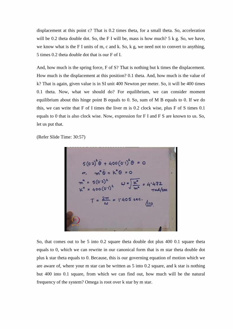
(Refer Slide Time: 30:57)

So, that comes out to be 5 into 0.2 square theta double dot plus 400 0.1 square theta

equals to 0, which we can rewrite in our canonical form that is m star theta double dot

plus k star theta equals to 0. Because, this is our governing equation of motion which we

are aware of, where your m star can be written as 5 into 0.2 square, and k star is nothing

but 400 into 0.1 square, from which we can find out, how much will be the natural

frequency of the system? Omega is root over k star by m star.

Now, if we put this values all are in S I units. So, no need to change anything anywhere.

The omega value comes out to be above 4.472 radian per second. And, how much will be

the period of vibration? T equals to 2 pi by omega which gives us 1.405 seconds is the

time period, natural time period of the system. So, that is the answer. This is the equation

of motion, which has been asked to derive in this problem. And, it has been asked, how

much is the natural period of vibration of the system? This is the natural period of

vibration of the system; that is the answer of the problem.

(Refer Slide Time: 33:14)

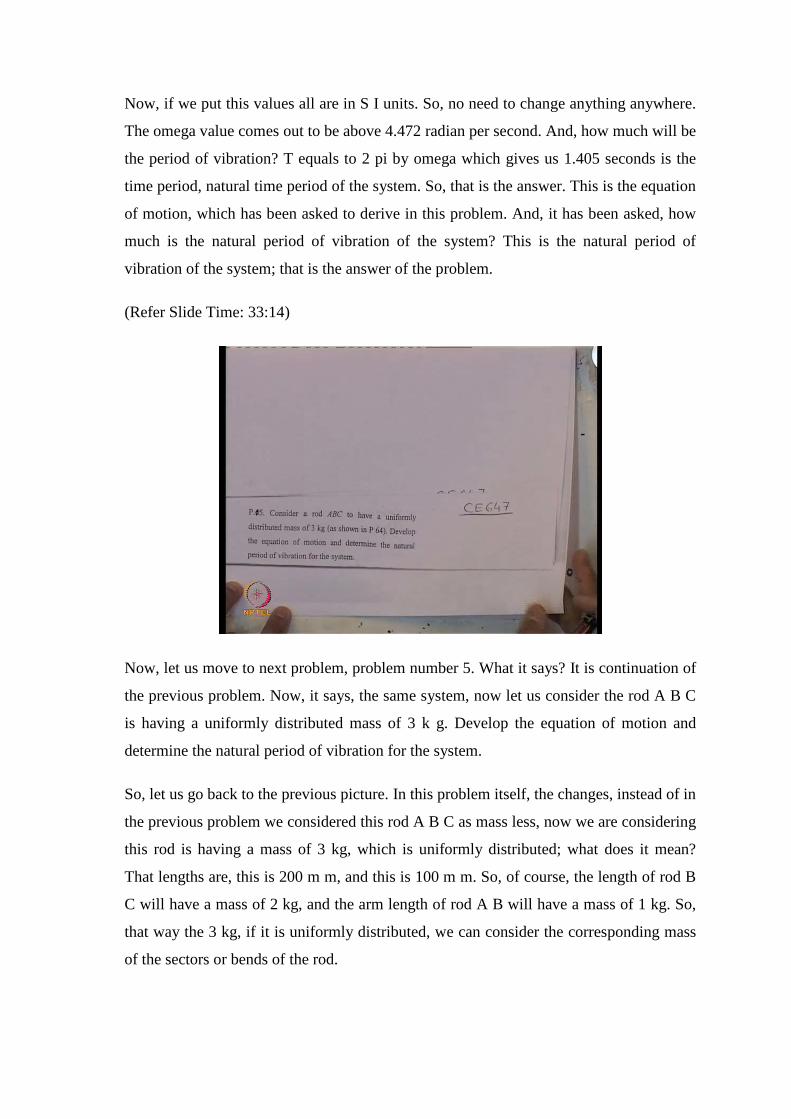
Now, let us move to next problem, problem number 5. What it says? It is continuation of

the previous problem. Now, it says, the same system, now let us consider the rod A B C

is having a uniformly distributed mass of 3 k g. Develop the equation of motion and

determine the natural period of vibration for the system.

So, let us go back to the previous picture. In this problem itself, the changes, instead of in

the previous problem we considered this rod A B C as mass less, now we are considering

this rod is having a mass of 3 kg, which is uniformly distributed; what does it mean?

That lengths are, this is 200 m m, and this is 100 m m. So, of course, the length of rod B

C will have a mass of 2 kg, and the arm length of rod A B will have a mass of 1 kg. So,

that way the 3 kg, if it is uniformly distributed, we can consider the corresponding mass

of the sectors or bends of the rod.

(Refer Slide Time: 34:51)

Now, if mass is uniformly distributed for a bar, how we compute the inertia of that bar

itself, let us look at it. So, whenever, we consider any bar which is having some

uniformly distributed mass; what are the inertia forces can act on this bar of length L

when it is subjected to vibration, there can be 3 different types of inertia force for this

bar. And, all this we consider at the centre of gravity of the bar, why? Because, all this

problems we are considering their masses are point mass.

So, if there is a acceleration, there is an acceleration in this direction say, x direction,

which is say, a x, the inertia force for this bar of uniformly distributed mass will be m

times a x in this direction; that is the horizontal inertia force. Similarly, if the bar is

subjected to a vertical acceleration of a y, in that case the inertia force in vertical

direction will be m times a y. Now, these are the translational inertia forces. If the bar is

rotated about its centre of gravity, in that case the rotational inertia force for a bar about

its centre is given by m L square by 12 times theta double dot, where theta is the angular

rotation, theta double dot is angular acceleration, and m L square by 12 is the moment of

inertia of the rod about its c g.

Now, the problem which has been given to us for this bar, let us look at it first; all this

forces are acting at the centre when we are assuming point mass, it is rotated by an angle

of theta. So, instead of considering that, it will have an inertia, rotational inertia force m

L square by 12 theta double dot acting at c g of the bar; what we can consider? That at

this end, at the end of the support where there is a support condition at the end, if we

want to transfer this to the support, how much it will be? It should be m L square by 12

plus L by 2 whole square mass; that much will give us m L square by 3 theta double dot

as the inertia force at the end. What does it mean? I am transferring this force from the

centre of the bar to one end of the bar that is it; it is the transfer of the force. So, we

know about this transfer of the force, how we can do.

So, instead of considering the inertia force at the c g, we can consider it at one end of the

bar also; that is what I wanted to show here; that if we considered the inertia forces at

one end of the bar rotational inertia force how much or how it should look like. And,

where from that force came? You did not ask me this one, but this is the force which I

have taken here, that m L by 2 into L by 2 that was the displacement at this point that is

why it came.

(Refer Slide Time: 40:02)

Now, coming to the solution of our problem, the free body diagram has to be changed

now, because we have the mass of the rod present in the system. So, let me draw the free

body diagram once again for this system, for a small rotation theta. Here one

concentrated mass of 5 k g from which we are getting the inertia force F I, here one

spring from which we are getting spring force F S, this length is 0.1 meter, this length is

0.2 meter, at this hinge support we can have B x and B y as support reactions at point B.

What else we can have here? Now, this rods are having mass, uniformly distributed mass

which can give us the inertia force; this has rotated in this direction. So, inertia force for

this component of the rod that is B C component, and this is A B component, this will be

how much say, F I 2, and this will be again another F I 3. This F I 2 and F I 3 are arising

because of the mass of this rod B C and A B.

Now, this F I and F S, we know their values, we have already computed, let us see how

much are the other two new inertia forces? F I 2 should be how much? It is m L square

by 3 theta double dot, right. So, how much is the mass for the rod B C? That is 2 k g. So,

2 into 0.2 whole square by 3 theta double dot is the F I 2. And, F I 3 will be, mass is 1 kg

for the rod A B times its distance square 0.1 square by 3 theta double dot. So, how the

equation of motion has changed now? The equation of motion if we rewrite, it will be F I

times 0.2.

So, we are writing sum of M B equals to 0, the same moment equilibrium about this

support point B. F I into 0.2 plus F I 2 plus F I 3 plus F S times 0.1 equals to 0. These are

the two additional inertia forces now we got; or, 5.2 square theta double dot is from this

expression we are getting F I 2 is 2 into 0.2 whole square by 3 theta double dot plus 1

into 0.1 square by 3 theta double dot plus 400 into 0.1 square equals to 0, which we can

rewrite in our canonical form m star theta double dot plus k star theta equals to 0.

(Refer Slide Time: 44:17)

Now, in this case, the expressions for m star is nothing but 5 into 0.2 whole square plus 2

into 0.2 whole square by 3 plus 1 into 0.1 whole square by 3 that is our m star; whereas,

k star remains as same like previous problem, 400 into 0.1 whole square. Knowing this

two, we can find out what is the natural frequency; it is root over k star by m star. If we

compute this value we will get, natural frequency is coming out to be 4.17 radian per

second, which will give us finally the natural period of vibration of the system as 1.5

seconds. Now, the governing equation of motion is this one, and natural period of

vibration is 1.5 second for this second problem.

What you can notice? Now, we can compare the previous problem result and this

problem result. What we got? The natural frequency in the previous problem was 4.472,

which has come down to 4.17 radian per second in the second problem, why? Because,

there is an increase in the mass. As the expression of omega suggest us, if there is an

increase in the mass, obviously, the natural frequency is going to decrease. So, that is

what has happened here also, as we can see. In other words, the natural time period has

increased from 1.405 to 1.5 seconds, because if the natural frequency is decreasing,

obviously, the natural period will increase, because it is the inverse of the frequency as

expected, fine.

(Refer Slide Time: 46:43)

Now, let us move to the next problem, problem number 6. Let us look at the problem

here; what it says? That one system is given here, it says, what are the differential

equation of motion about the static equilibrium configuration and the natural frequency

of motion of the body A, so, this is the body A, for a small motion of this rod B C. But it

says, neglect the inertial effects from B C. So, it is assumed to be as mass less. And,

consider the values of this spring constant k 1 as 15 Newton per meter, k 2 as 20 Newton

per meter, and k 3 30 Newton per meter, and weight of this body or point mass is 30

Newton. So, that is the problem statement. So, let us see, now, how we can formulate the

equation of motion for this problem.

(Refer Slide Time: 47:53)

Let us draw the free body diagram of the system. Let us draw the free body diagram for

this rod B C. So, C is your support, hinge support for a small rotation; this is our

direction of motion we are considering at any instant of time; this is end B; this is end C,

which is hinged. Here one spring was connected. So, of course, if it is rotated by an angle

theta, some spring force will come from this side. So, let us denote that spring force as F

S 3.

And, subsequently if one spring force is coming at this point, at this midpoint also

another spring is connected here, as you can look here. That also has gone through

displacement here. So, another spring force will act at this point as well, to bring it back

to its original position. So, let us denote that as F S 2. Now, how much at the values of

this F S 3? F S 3 is K 3 times the distance B C times theta; or, let us say, this

displacement we are denoting as y of B. So, it can be written as K 3 times y of B. Now,

values of k 3 is given to us, 30 Newton per meter. So, 30 y of B.

How much should be the, this displacement at the midpoint, this point is midpoint; as per

figure this is 3 meter, this is also 3 meter. So, this should be y B by 2, right. So, F S 2,

how we can compute? F S 2 will be the spring constant K 2 times this displacement, no

not this displacement, because look at the other end of the spring, see for this spring, the

force is k 3 times y B, because the other end was fixed end. In this case, the other end of

the spring k 2, is not a fixed end. So, there also can be some movement, and the spring

force in k 2 should be the relative displacement between the two ends. So, it is better, if

we draw the free body diagram of the spring two; that will give us a better picture. So, at

this end, we have F s 2 acting in this direction, F s 2 acting in this direction. So, I am

drawing the free body diagram of the spring two.

And, how much is the displacement of this end, is y B by 2 in downward direction. Let

us assume that at end A its displacement is y A in downward direction. So, F s 2 will be

k 2 times the relative displacement y B by 2 minus y A. Now, value of k 2 is given to us,

which is 20 Newton per meter. So, 20 times y B by 2 minus y A. Now, for this sector B

C, or rod B C, we can now write down the moment equilibrium about this support C,

hinge support C. What it should give? Sum of m C equals to 0, which means F s 3 times

6, because this is 3 meter, this is also 3 meter. So, F s time 6 clockwise plus F s 2 times 3

equals to 0.

Now, if we put the expression of F s 3 and F s 2 in this equation of moment equilibrium,

what we will get? We will get a relationship between y B and y A; that gives us on

simplification y B comes out to be 2 seventh of y A. So, after getting this relation, let us

now go back to that point mass A, and draw, try to draw the free body diagram of point

mass A. So, for point mass A, the free body diagram should be now, there is a spring

force F s 2 in this direction, why it should be in this direction? Let us go back to the

previous free body diagram for this spring, at this end force was upward direction. So, to

maintain the equilibrium at this point, obviously, the direction will be downward.

(Refer Slide Time: 54:18)

And, the deflection of point A, we have considered downward as y A; there will be

another spring force which is F s 1 for the presence of the spring k 1 here, with another

end does the fixed end. And, as this is the mass, it will be subjected to an acceleration,

because of the vibration it will have an inertia force also. So, inertia force also will act.

As the movement is considered in the downward direction, it will try to bring in back its

original positions. So, that is why the direction F I is vertically upward.

If it is so, how much will be our F of I for this free body diagram, mass times

acceleration; how much is acceleration? y A double dot is the acceleration. How much is

the mass? Weight of the body A is given as 30 Newton. So, mass will be 30 divided by

9.81 is the mass, times y A double dot, is a inertia force. And, how much is the spring

force F s 1? That is k 1, spring constant k 1 times the relative displacement that is y A

only. Because, the other end is fixed end. Now, k A value is given to us, 15 Newton per

meter. So, 15 y A.

Now, what we should do, now for this free body diagram? We should use D’Alembert’s

principle, which we can write as F s 2 equals to F I plus F s 1. D’Alembert’s principle

says that all the forces will remain in equilibrium, when any object is in vibration. So,

that is what, using this equilibrium condition, now we can put our equation in the known

canonical form; by putting expressions for all the known parameters, m star y A double

dot plus k star y A equals to 0.

Now, if you put all the values of this known parameters here, we will get the natural

frequency as root over k star by m star, which if you compute, you will get 3.242 radian

per second. So, that is the answer. It was asked that what is the natural frequency of

motion at this system. So, this is our answer, fine. Now, let us move to the next problem,

problem number 7. So, we will do that problem in the next lecture, we will stop here

today.