100 nm Kaolinite Todorokite Birnessite Lepidocrocite Calcite Siderite Pyrite Gypsum Jarosite Hematite Goethite Barite Ferrihydrite Maghemite H C Na Mg Al Si Mica Halloysite Quartz XRD TEM SEM Opal-CT Zeolite P S K Ca Mn Fe Smectite c a b d Soil Mineralogy Fall 2009 Youjun Deng, G. Norman White, and Joe B. Dixon Laboratory Manual
Transcript
100 nm
KaoliniteTodorokite BirnessiteLepidocrocite
Calcite
Siderite
Pyrite
GypsumJarosite
Hematite
Goethite
Barite
Ferrihydrite
Maghemite
H
C
Na
Mg Al Si
Mica
Halloysite
Quartz
XRD
TEM
SEM
Opal-CT
Zeolite
P
S
K
Ca
Mn
Fe
Smectite
c
a b
d
Soil Mineralogy
Fall 2009
Youjun Deng, G. Norman White, and Joe B. Dixon
Laboratory Manual
Tell me and I will forget,Show me and I will remember,
Involve me and I will understand.
This manual is designed for use in instruction and research devoted to solving problemsinvolving clays, soils, and sediments in soil science, geology, oceanography, civil engineering, andenvironmental sciences.
i
About the Cover
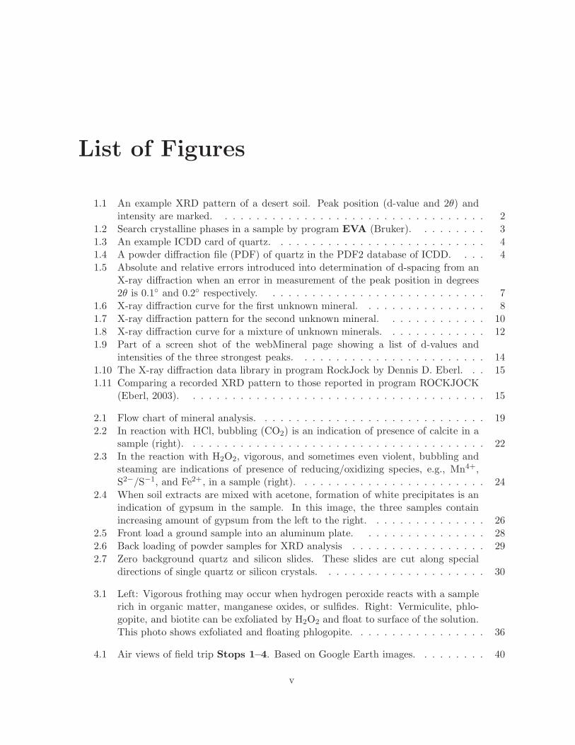
The cover illustrates the composition of the Soil Mineralogy course. Early in the course, there isa local field trip and study some 20 core minerals. On the field trip, you will see a soil profile anddiscuss important soil terms to help the class develop a similar terminology base. The Burlesonsoil profile sketch (a) illustrates the systematics of naming soil horizons and it illustrates howdiverse soils can be. The x-ray diffraction curves (b) represent a real curve obtained from a clayfraction and a model curve calculated to match it using the Newmod software employed in thecourse. The fibrous clay illustrated in a transmission electron micrograph (c) depicts a rare formof fibrous halloysite and the platy kaolinite (d) represents a common mineral of similar structureto halloysite yet it has grossly different morphology and particle size. This diversity of crystalshape and size illustrate the range of properties of minerals in soils in one structural group.
The twenty core mineral names are arrayed in the margin of the page grouped by composi-tion or structural type. The minerals seen in the field illustrate the variety of minerals in soilsand sediments in various chemical and structural groups e.g. carbonates, sulfates, oxides, andsilicates. The instruments used in the course to identify and characterize the minerals presentin student samples are abbreviated in the margin too. The chemical elements that receiveparticular attention in the course also are abbreviated in the array in the margin.
Acknowledgements
We would like to thank the students of Soil Mineralogy at Texas A&M University and others whohave brought the shortcomings of earlier versions of these lab exercises to our attention eitherverbally or by example. The authors also appreciate the cooperation and use of facilities of theTexas A&M University Electron Microscopy Center. The simulated X-ray diffraction patternsin this manual were calculated with the NEWMOD computer program of R.C. Reynolds.
For Reference:
Deng, Y., G. N. White, and J. B. Dixon. 2009. Soil Mineralogy Laboratory Manual.11th edition. Published by the authors, Department of Soil and Crop Sciences, Texas A&MUniversity, College Station, Texas 77843-2474.
15 Integrating Different Data for Quantification 17915.1 Quantitative Analysis of Clays Using CEC, Total K, and NEWMOD . . . . . . . 17915.2 Further Quantification Using NEWMOD . . . . . . . . . . . . . . . . . . . . . . . 180
List of Figures
1.1 An example XRD pattern of a desert soil. Peak position (d-value and 2θ) andintensity are marked. . . . . . . . . . . . . . . . . . . . . . . . . . . . . . . . . . 2
1.2 Search crystalline phases in a sample by program EVA (Bruker). . . . . . . . . 31.3 An example ICDD card of quartz. . . . . . . . . . . . . . . . . . . . . . . . . . . 41.4 A powder diffraction file (PDF) of quartz in the PDF2 database of ICDD. . . . 41.5 Absolute and relative errors introduced into determination of d-spacing from an
X-ray diffraction when an error in measurement of the peak position in degrees2θ is 0.1◦ and 0.2◦ respectively. . . . . . . . . . . . . . . . . . . . . . . . . . . . 7
1.6 X-ray diffraction curve for the first unknown mineral. . . . . . . . . . . . . . . . 81.7 X-ray diffraction pattern for the second unknown mineral. . . . . . . . . . . . . 101.8 X-ray diffraction curve for a mixture of unknown minerals. . . . . . . . . . . . . 121.9 Part of a screen shot of the webMineral page showing a list of d-values and
intensities of the three strongest peaks. . . . . . . . . . . . . . . . . . . . . . . . 141.10 The X-ray diffraction data library in program RockJock by Dennis D. Eberl. . . 151.11 Comparing a recorded XRD pattern to those reported in program ROCKJOCK
2.1 Flow chart of mineral analysis. . . . . . . . . . . . . . . . . . . . . . . . . . . . . 192.2 In reaction with HCl, bubbling (CO2) is an indication of presence of calcite in a
sample (right). . . . . . . . . . . . . . . . . . . . . . . . . . . . . . . . . . . . . . 222.3 In the reaction with H2O2, vigorous, and sometimes even violent, bubbling and
steaming are indications of presence of reducing/oxidizing species, e.g., Mn4+,S2−/S−1, and Fe2+, in a sample (right). . . . . . . . . . . . . . . . . . . . . . . . 24
2.4 When soil extracts are mixed with acetone, formation of white precipitates is anindication of gypsum in the sample. In this image, the three samples containincreasing amount of gypsum from the left to the right. . . . . . . . . . . . . . . 26
2.5 Front load a ground sample into an aluminum plate. . . . . . . . . . . . . . . . 282.6 Back loading of powder samples for XRD analysis . . . . . . . . . . . . . . . . . 292.7 Zero background quartz and silicon slides. These slides are cut along special
directions of single quartz or silicon crystals. . . . . . . . . . . . . . . . . . . . . 30
3.1 Left: Vigorous frothing may occur when hydrogen peroxide reacts with a samplerich in organic matter, manganese oxides, or sulfides. Right: Vermiculite, phlo-gopite, and biotite can be exfoliated by H2O2 and float to surface of the solution.This photo shows exfoliated and floating phlogopite. . . . . . . . . . . . . . . . . 36
4.1 Air views of field trip Stops 1–4. Based on Google Earth images. . . . . . . . . 40
v
vi
4.2 A Boonville soil profile at Stop 1 and complex mixture of minerals in the soil. . 414.3 An eroded landscape at Stop 2. Nearly pure jarosite and goethite-rich particles
are exposed to the surface. . . . . . . . . . . . . . . . . . . . . . . . . . . . . . . 424.4 Petrified wood with various sizes can be found along the eroded landscape at
4.7 Summary of the proposed major processes affecting the volcanic ash followingdeposition in the swamp: Zeolite = clinoptilolite. From Senkayi et al. (1984). . . 46
4.8 Scanning electron micrographs showing (a) vermicular kaolinite (indicated byarrow), (b) books of kaolinite in tonstein, (c) leafy crystallites of smectite inthe bentonite, and (d) clinoptilolite crystals in the underlying lignitic bed. Theclinoptilolite crystals show the typical coffin-shape morphology. After Senkayiet al. (1984). . . . . . . . . . . . . . . . . . . . . . . . . . . . . . . . . . . . . . . 46
4.9 lenticular siderite rocks showing siderite and weathering products (manganeseoxides and iron oxides) of the rock. . . . . . . . . . . . . . . . . . . . . . . . . . 47
4.10 Iron oxides, including magnetic maghemite, on the road surface between Stops2 and 3. . . . . . . . . . . . . . . . . . . . . . . . . . . . . . . . . . . . . . . . . 48
4.11 Various iron oxides precipitate along plant root and cracks at Stop 4. . . . . . 49
5.1 Setup for sand separation by wet sieving. . . . . . . . . . . . . . . . . . . . . . . 525.2 Clay particles (< 2 μm) in the sieved suspension (< 53 μm, left) are separated by
sedimentation or centrifugation methods and are collected in a 750-mL (or 1000-mL) centrifuge bottle (middle). Fine clay particles (< 0.2 μm) are separated bycentrifugation and are collected in a larger container (e.g., 5-L beaker). . . . . . 57
5.3 A particle settles in a fluid by its own weight. . . . . . . . . . . . . . . . . . . . 585.4 A particle settles in a fluid by centrifugation. . . . . . . . . . . . . . . . . . . . . 61
6.1 Left: Clay suspension is pipetted onto a glass disc and air dried to make anoriented clay film; Middle: Place a very small amount of reusable poster adhesiveat four locations of a holder, line up the surface of the clay film with the rim bypressing the disc down to the cavity with another holder with a slightly smallercavity; Right: A mounted disc. . . . . . . . . . . . . . . . . . . . . . . . . . . . . 70
6.2 The effects of domain thickness on the XRD patterns for kaolinite as calculatedusing NEWMOD. . . . . . . . . . . . . . . . . . . . . . . . . . . . . . . . . . . . 73
6.3 Calculated NEWMOD patterns for mica/smectite interstratifications. Only theMg and Mg glycerol patterns are shown because the other patterns would beidentical. . . . . . . . . . . . . . . . . . . . . . . . . . . . . . . . . . . . . . . . . 75
6.4 X-ray diffraction patterns for the coarse clay fraction from a weathered rockbeneath a bauxite mine in Arkansas (sample provided by S. D. Walling). . . . . 77
6.5 X-ray diffraction patterns for an unfractionated Pacific Ocean sediment (sampleprovided by P. J. Burkett). . . . . . . . . . . . . . . . . . . . . . . . . . . . . . . 78
vii
6.6 X-ray diffraction pattern for fine clay from a Beaumont clay soil of SoutheastTexas (sample provided by M. G. Goube). . . . . . . . . . . . . . . . . . . . . . 79
6.7 X-ray diffraction curves for the coarse clay fraction from a black pyritiferous shale(sample provided by O. Kwon). . . . . . . . . . . . . . . . . . . . . . . . . . . . 80
6.8 X-ray diffraction curves for the coarse clay from a sedimentary rock from westTexas (sample provided by J. P. Harris). . . . . . . . . . . . . . . . . . . . . . . 81
6.9 X-ray diffraction curves for the coarse clay fraction from the lignite overburdenof a mine in east Texas (sample provided by Yao Li). . . . . . . . . . . . . . . . 82
6.10 X-ray diffraction curves for the coarse clay fraction from a kaolinitic Honduransoil (sample provided by J. O. Caldwell). . . . . . . . . . . . . . . . . . . . . . . 83
6.11 X-ray diffraction curves for the fine clay fraction from a Bazette soil from north-east Texas (sample provided by D. K. Marquart). . . . . . . . . . . . . . . . . . 84
6.12 X-ray diffraction curves for the coarse clay fraction from a Reagan-Hodgins soilseries association of west Texas (sample provided by M. E. West). . . . . . . . . 85
6.13 X-ray diffraction curves for the fine clay fraction from a Bastsil soil from centralTexas (sample provided by L. C. Nordt). . . . . . . . . . . . . . . . . . . . . . . 86
7.1 Bragg condition for X-ray diffraction. The scattered X-rays from all of the (hkl)planes are in phase, that is, 0 or n2π phase difference. The path difference of thescattered X-rays from two adjacent (hkl) planes is 2d sin θ. . . . . . . . . . . . . 88
7.2 Schematic representation of X-ray diffraction and the major optics in Bragg-Brentano configuration. . . . . . . . . . . . . . . . . . . . . . . . . . . . . . . . . 89
7.3 A Bruker D8 ADVANCE X-ray diffractometer equipped with an auto samplechanger, a rotating sample stage, and three detectors: an energy dispersive de-tector (Sol-X), a fast one-dimensional position sensitive detector (LynxEye), anda conventional scintillation detector. . . . . . . . . . . . . . . . . . . . . . . . . . 89
7.4 A sealed X-ray tube and schematic view of the cross section of the tube. (Photosource: PANalytical) . . . . . . . . . . . . . . . . . . . . . . . . . . . . . . . . . 90
7.5 Continuous and characteristic X-ray radiation for copper at different operatingvoltages. The left panel is modified from Jenkins and Snyder (1996). . . . . . . 91
7.6 Generation of white (continuous) X-ray radiation by bremsstahlung. . . . . . . . 917.7 Generation of photoelectron, characteristic Kα and Kβ X-rays, and Auger elec-
tron when an atom is irradiated with an electron or photon beam. Based onJenkins and Snyder (1996). . . . . . . . . . . . . . . . . . . . . . . . . . . . . . . 92
7.8 Unwanted kβ and fluorescence X-ray can be filtered out with a monochromator. 937.9 Quantitative analysis of mineral composition based on Rietveld refinement. This
example shows the observed and calculated XRD patterns and their difference of asample taken from a cinder cone in the Haleakala crater valley, Maui, Hawaii. Thecalculation was conducted with software TOPAS by Dr. Holger Cordes (Bruker). 96
7.10 Observed and calculated XRD patterns and their difference in program FullPat(Chipera and Bish, 2002). . . . . . . . . . . . . . . . . . . . . . . . . . . . . . . 97
9.1 Schematic representation of the electromagnetic spectrum. Modified from Ad-vanced Light Source, Lawrence Berkeley National Laboratory (http://www-als.lbl.gov/als/quickguide/vugraph.html, accessed in December 2007). . . . . . . . . 116
9.2 Schematic representation of possible tetrahedral vibrations. Arrows representthe direction of movement in the plane of the paper and the + and - representmovements above and below the plane of the paper, respectively. . . . . . . . . 117
9.3 A Fourier transform infrared spectrometer Spectrum 100 from PerkinElmer. Themodular sample accessories are exchangeable on the instrument. This figure showsaccessories for diffuse reflectance (DRIFT), universal attenuated total reflection(ATR, diamond-zinc selenate), horizontal ATR (HATR), and transmission anal-yses. (Image source: PerkinElmer, Inc.) . . . . . . . . . . . . . . . . . . . . . . . 120
9.4 The DRIFT design on Spectrum 100. (Image source: PerkinElmer, Inc.) . . . . 1219.5 Sample cups with different sizes, abrasive pads or sticks can be used to mount
samples in DRIFT. (Image source: PerkinElmer, Inc.) . . . . . . . . . . . . . . . 1219.6 Diffuse reflectance infrared spectra for a soil coarse clay fraction from a fine,
montmorillonitic, hyperthermic Vertic Argiudoll showing the effects of sampleconcentration on the quality of the infrared pattern. Note the better band ex-pression on the top pattern that was 10 fold less concentrated. Sample providedby Gad Ritvo. . . . . . . . . . . . . . . . . . . . . . . . . . . . . . . . . . . . . . 122
9.9 Diffuse reflectance (DR) Fourier transform infrared (FTIR) pattern for a sampleobtained from the type location for Fithian illite in Illinois (Il05). . . . . . . . . 131
10.1 Comparison of optical microscope to transmission and scanning electron micro-scopes. From JEOL (2006). . . . . . . . . . . . . . . . . . . . . . . . . . . . . . 134
10.2 Electron beam-sample interactions and emitted electrons and photons (left); anddepth of quantum generation and space resolution (Right). After Goldstein et al.(1992) and JEOL (2006). . . . . . . . . . . . . . . . . . . . . . . . . . . . . . . . 135
10.3 Force on a moving electron in a magnetic field. According to Geiss (1979). . . . 13610.4 Trajectories of (a) a single electron and (b) a group of electrons passing through
an electromagnetic lens. From Bozzola and Russell (1992). . . . . . . . . . . . . 13610.5 Scanning electron microscopy graphs of sands of a sediment etched with alkaline
solution. Images were recorded with secondary electron signals. . . . . . . . . . 13710.6 Energies of characteristic X-rays of elements. From EDAX. . . . . . . . . . . . . 138
10.8 Backscatter SEM image of a phosphate-bearing nodule. Backscatter imaginghighlights contrast in atomic number, thus enabling the quartz grains to be read-ily distinguished as the darker shapes embedded in the lighter (Fe- and P-rich)matrix. From Harris (2002). . . . . . . . . . . . . . . . . . . . . . . . . . . . . . 140
10.9 (a) SEM image of a kaolinite crystal; (b) electron backscattered diffraction (EBSD)pattern of the kaolinite crystal; and (c) calculated Kikuchi pattern correspondingto the EBSD pattern in b. The black arrows in b and c indicate the characteristic±(110) Kikuchi band of kaolinite. From Kameda et al. (2005) . . . . . . . . . . 141
11.1 (a) Transmission electron microscope as viewed by a user; (b) comparative ar-rangement of electron diffraction and (c) X-ray diffraction to show sample tobeam relationships in both cases. The electron beam passes through the sampleand the X-ray beam strikes the surface of the sample at an acute angle. A 2θ re-lationship exists for both diffraction systems. Data obtained by the two methodscomplement each other because of different beam to sample arrangements. . . . 154
11.2 Goethite crystal fragment from Biwabik, Minnesota with insets of enlarged latticefringes and a single crystal electron diffraction pattern. . . . . . . . . . . . . . . 155
11.3 Moire patterns in Beaumont soil 0.2-2 μm clay. From Dixon (1978). . . . . . . . 15611.4 Holey Carbon film with fine Mg oxide particles on it. This type of film is used to
mount small particles for high resolution transmission electron microscopy. . . . 15711.5 Transmission electron micrograph of bentonite from Australia (34AU) survey mi-
crograph illustrating a natural mixture of salt crystals identified morphologicallyas halite cubes, halloysite tubes, a 1:1 layer silicate with rolled structural layersand interlayer water, and the background of thin smectite sheets visible throughthe holey carbon support grid. . . . . . . . . . . . . . . . . . . . . . . . . . . . . 158
11.6 a. Goethite twin with four arms with blunt ends and b. Numerous lattice fringesand distinct crystal faces on the right and top edges. Even though the particlesare extremely small the lattice fringes are crisp and visible. (Dixon, 1999). . . . 159
11.7 Electron diffraction by (hkl) planes of a crystal with a parallel electron beam.Direction change of the source electron beam due to scattering will be consideredlater. . . . . . . . . . . . . . . . . . . . . . . . . . . . . . . . . . . . . . . . . . . 160
x
List of Tables
1.1 Peak locations and heights for the unknown mineral in the X-ray diffraction pat-tern shown in Fig. 1.6. . . . . . . . . . . . . . . . . . . . . . . . . . . . . . . . . 9
1.2 Peak locations and heights for the unknown mineral in the X-ray pattern shownin Fig. 1.7. Note that the first two peaks chosen by the computer are not real. . 11
1.3 Peak locations and intensities for the X-ray diffraction pattern of the unknownmixture. Note first 3 peaks chosen by the computer are not real. The actualpattern with labeled corresponding to the table is in Fig. 1.8. . . . . . . . . . . 13
5.1 Settling time (by gravity) for particles with diameters of 2 and 20 μm to fall8.5 cm in water∗. . . . . . . . . . . . . . . . . . . . . . . . . . . . . . . . . . . . 60
6.1 The d(001)-spacings of phyllosilicate minerals after different cation saturation,solvation, and heat treatments. Modified from Whittig (1965). . . . . . . . . . . 72
9.1 Infrared absorption frequency regions for layer silicates (Farmer, 1974a). . . . . 1269.2 Infrared absorption bands for selected soil minerals. Modified after White (1971). 1279.3 Wavenumber locations for OH-stretching bands for common cation pair combi-
nations in dioctahedral micas. From Slonimskaya et al. (1986). . . . . . . . . . . 1289.4 Frequencies of OH-stretching bands from some phyllosilicates (from White, 1971). 1289.5 Frequencies of OH-bend bands for selected octahedral cation occupancies. Data
from White (1971) and Farmer (1974a). . . . . . . . . . . . . . . . . . . . . . . . 129
10.1 Qualitative peak ratio correction factors for metal to silicon peaks from EDS data.Multiply the factor with the peak ratio to get a molar ratio. Larger factors meanthat a smaller peak is needed to be equimolar with silicon. . . . . . . . . . . . . 145
10.2 Recognition criteria used for mineral identification for soil minerals observed bySEM. Minerals are arranged in an approximate order of decreasing frequency ofoccurrence in developed soils. Other minerals may occur in soils but their mor-phology and chemistry is not distinctive enough for use in mineral identificationwithout corroborating XRD data. Elements above Na are assumed detectable byEDS. . . . . . . . . . . . . . . . . . . . . . . . . . . . . . . . . . . . . . . . . . . 145
11.1 Electron diffraction angles (θ) at 200 kV accelerating voltage. . . . . . . . . . . 15911.2 Transmission Electron Microscopy (TEM) Preparation and Records Form. . . . 163
xi
xii
Chapter 1
Introduction to MineralIdentification Using XRD
1.1 Introduction
Identifying minerals is the first step in mineral analysis. Sometimes, one single analytical methodis sufficient to accomplish the job, and sometimes, several analytical techniques have to be em-ployed. Among commonly-used methods, X-ray diffraction (XRD) has been proven to be indis-pensable. In this exercise, we will focus on mineral identification using XRD; in latter chapters,we will exercise mineral identification using infrared spectroscopy and electron microscopies.
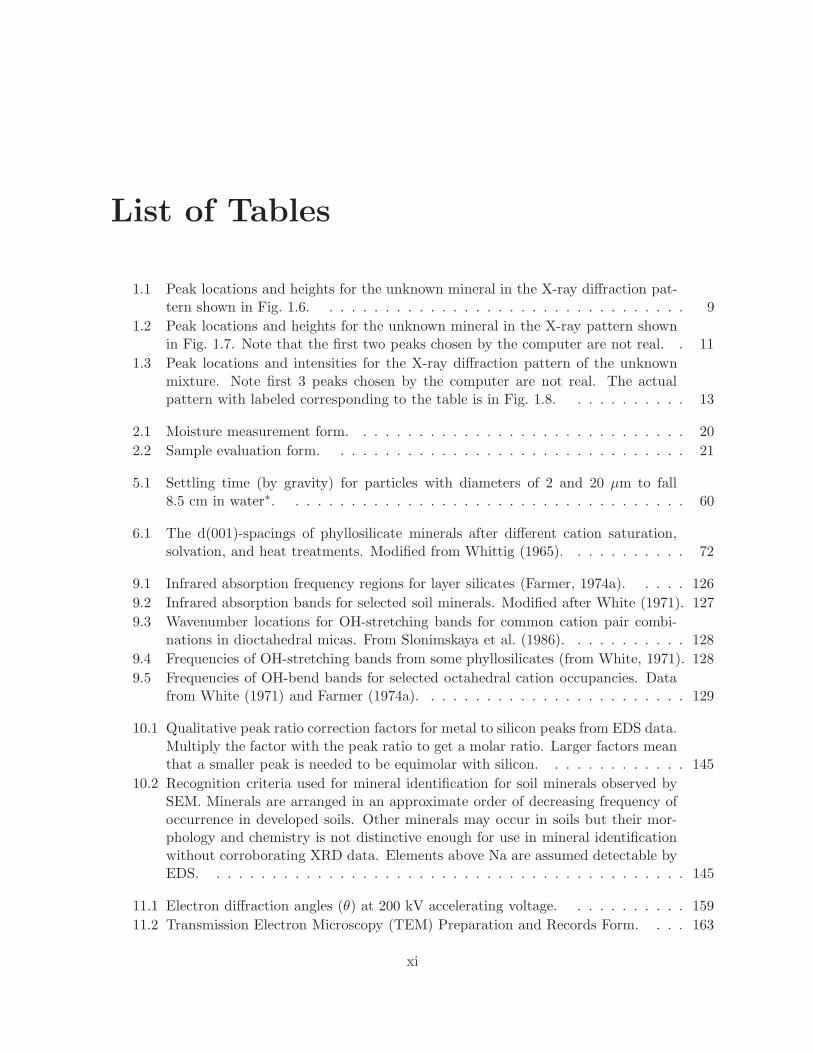
Fig. 1.1 is an example X-ray diffraction pattern recorded with Cu Kα X-ray radiation.The y-axis of an XRD pattern is in some measure of peak intensity, usually counts, counts persecond, or relative intensity. The x-axis gives the diffraction 2θ angles, which can be convertedto interplanar spacings d using Bragg’s Law.
nλ = 2d sin θ (1.1)
where λ is the wavelength of the X-ray, θ is the diffraction angle, d is the distance between twoadjacent diffracting lattice planes, and n is an integer stands for the order of diffraction.
1.2 Computer-aided Mineral Phase Identification
Many X-ray diffraction data processing softwares can perform automated mineral search/matchby comparing a recorded pattern to those stored in the International Centre for DiffractionData (ICDD) database, formerly known as Joint Committee on Powder Diffraction Standards(JCPDS). A user can set certain criteria such as chemical composition of a sample and names ofpossible minerals to narrow down the search range (e.g., Fig. 1.2). Normally, the softwares findseveral possible minerals and ask the user to pick up the best match. If a sample contains manycrystalline phases, the search/match is more difficult. Very often, the computer reports someunlikely minerals and also misses some very obvious phases as well. Better knowledge aboutthe sample and some experience with XRD patterns of known minerals will greatly enhance theaccuracy of mineral identification. For most soil and sediment samples, it is unlikely that theycontain too many unusual minerals and therefore, guess-and-check is probably one of the mostoften used strategy in computer aided mineral identification.
1
2
0
2000
4000
6000
8000
10000
2-Theta (degrees)2 10 20 30 40 50 60
2th=
63.9
4 °,
d=1.
455,
I=66
1 C
ps
2th=
62.3
5 °,
d=1.
488,
I=49
7 C
ps2t
h=61
.72
°,d=
1.50
2,I=
650
Cps
2th=
59.9
9 °,
d=1.
541,
I=11
49 C
ps
2th=
58.7
3 °,
d=1.
571,
I=41
1 C
ps
2th=
57.4
6 °,
d=1.
602,
I=44
1 C
ps2t
h=56
.63
°,d=
1.62
4,I=
394
Cps
2th=
55.9
2 °,
d=1.
643,
I=47
2 C
ps2t
h=55
.38
°,d=
1.65
8,I=
531
Cps
2th=
54.8
6 °,
d=1.
672,
I=79
5 C
ps2t
h=54
.25
°,d=
1.69
0,I=
402
Cps
2th=
53.2
4 °,
d=1.
719,
I=42
0 C
ps2t
h=52
.58
°,d=
1.73
9,I=
328
Cps
2th=
51.2
9 °,
d=1.
780,
I=44
0 C
ps2t
h=50
.67
°,d=
1.80
0,I=
614
Cps
2th=
50.1
0 °,
d=1.
819,
I=18
63 C
ps2t
h=49
.14
°,d=
1.85
2,I=
398
Cps
2th=
48.5
3 °,
d=1.
874,
I=42
7 C
ps
2th=
47.4
5 °,
d=1.
915,
I=40
8 C
ps2t
h=47
.08
°,d=
1.92
9,I=
348
Cps
2th=
45.7
8 °,
d=1.
980,
I=72
8 C
ps2t
h=44
.75
°,d=
2.02
4,I=
333
Cps
2th=
43.2
0 °,
d=2.
093,
I=49
5 C
ps2t
h=42
.45
°,d=
2.12
8,I=
923
Cps
2th=
41.7
0 °,
d=2.
164,
I=49
9 C
ps2t
h=40
.79
°,d=
2.21
0,I=
322
Cps
2th=
40.2
6 °,
d=2.
238,
I=58
9 C
ps2t
h=39
.46
°,d=
2.28
2,I=
952
Cps
2th=
38.4
9 °,
d=2.
337,
I=32
6 C
ps2t
h=37
.64
°,d=
2.38
8,I=
456
Cps
2th=
37.0
5 °,
d=2.
424,
I=51
2 C
ps2t
h=36
.55
°,d=
2.45
6,I=
933
Cps
2th=
36.0
4 °,
d=2.
490,
I=55
5 C
ps2t
h=35
.48
°,d=
2.52
8,I=
617
Cps
2th=
34.9
9 °,
d=2.
562,
I=70
6 C
ps2t
h=34
.45
°,d=
2.60
1,I=
541
Cps
2th=
33.8
5 °,
d=2.
646,
I=36
5 C
ps2t
h=33
.05
°,d=
2.70
8,I=
332
Cps
2th=
32.2
9 °,
d=2.
770,
I=30
5 C
ps2t
h=31
.38
°,d=
2.84
9,I=
437
Cps
2th=
30.8
5 °,
d=2.
896,
I=47
0 C
ps2t
h=30
.40
°,d=
2.93
8,I=
657
Cps
2th=
29.8
5 °,
d=2.
991,
I=57
6 C
ps2t
h=29
.42
°,d=
3.03
4,I=
900
Cps
2th=
28.4
5 °,
d=3.
135,
I=64
5 C
ps2t
h=27
.91
°,d=
3.19
4,I=
2920
Cps
2th=
27.5
0 °,
d=3.
241,
I=18
35 C
ps2t
h=26
.65
°,d=
3.34
2,I=
6827
Cps
2th=
25.5
9 °,
d=3.
479,
I=56
5 C
ps
2th=
24.2
5 °,
d=3.
668,
I=59
2 C
ps2t
h=23
.60
°,d=
3.76
6,I=
710
Cps
2th=
23.0
1 °,
d=3.
863,
I=33
4 C
ps2t
h=21
.99
°,d=
4.03
9,I=
829
Cps
2th=
20.8
5 °,
d=4.
256,
I=13
53 C
ps
2th=
19.7
7 °,
d=4.
486,
I=46
7 C
ps
2th=
17.7
0 °,
d=5.
006,
I=13
9 C
ps
2th=
15.8
3 °,
d=5.
593,
I=10
2 C
ps2t
h=15
.03
°,d=
5.88
9,I=
115
Cps
2th=
13.7
7 °,
d=6.
427,
I=15
9 C
ps
2th=
12.3
7 °,
d=7.
149,
I=13
3 C
ps
2th=
10.4
4 °,
d=8.
470,
I=20
3 C
ps
2th=
8.76
°,d
=10.
089,
I=28
8 C
ps
2th=
6.19
°,d
=14.
268,
I=21
3 C
psInte
nsity
(Cou
nts/
seco
nd)
Figure 1.1. An example XRD pattern of a desert soil. Peak position (d-value and 2θ)and intensity are marked.
1.3 Use Search Manual to Identify Minerals
Identifying minerals via manual search was a common practice in mineral identification in thepast and it still has its merits. This is particularly true when you are dealing with a complexmixture such as a soil or a sediment sample in which the diffraction peaks of minor crystallinephases are too weak and therefore, be ignored by the computer in the automated search/matchanalysis.
The Mineral Powder Diffraction File Search Manual contains ordered lists of entries designedfor comparison to measured d-spacings and intensities obtained from XRD data collected bymany methods. The search lists in the manual are based on a selection of XRD patternscontained in a set of books called the ICDD (formerly JCPDS) X-ray Powder Data Files. Inthese books, minerals are arranged in alphabetical order by name in recent editions but arearranged in numerical order by set number in the earlier editions. The books contain list ofpeak intensities obtained from XRD patterns of samples assumed to consist of only one mineralor from a sample with a limited number of impurities from which any peaks resulting fromother minerals were not listed. The individual patterns are in a set format called a card becauseoriginally they were available on cards for a different manual search method. The cards arenumbered with the set number followed by a dash and then another number referring to theindividual pattern, such as the quartz pattern is 5-0490.
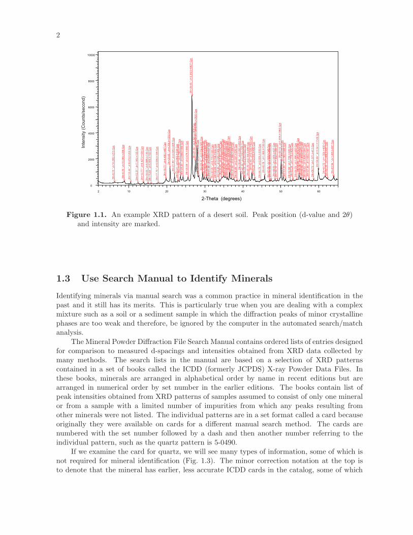
If we examine the card for quartz, we will see many types of information, some of which isnot required for mineral identification (Fig. 1.3). The minor correction notation at the top isto denote that the mineral has earlier, less accurate ICDD cards in the catalog, some of which
3
Figure 1.2. Search crystalline phases in a sample by program EVA (Bruker).
are listed at the bottom left in the card. The top row of the card, starting with d, followed by3.34, 4.26, 1.82, and 4.26 are the listing for the d-spacings for the most intense peaks startingwith the most intense at the left. The second row lists the intensities for these peaks relativeto the most intense peak (100%). These peaks and their intensities are those used in the searchmanuals. The box to the right of these two rows contains the chemical formula written two waysand the name of the mineral. The star at the top right of the box indicates the data on thecard has high reliability; other symbols denote decreasing reliability. The box directly belowthe box with d-spacings and intensities for the strongest peaks contain data about the data.The CuKα1 means that the data was collected using CuKα1 radiation, which has a wavelength,λ, of 1.5405 Angstroms (A). To obtain this radiation the Cu radiation was filtered with a Nifilter, which would reduce the contribution of other forms of Cu radiation that have differentwavelengths. The data was collected using a diffractometer, much like the data for this course,and came from reference National Bureau of Standards (NBS) Circular. The next box belowcontains crystallographic data for the mineral, with a box below containing optical propertiesfor the mineral, with the bottom box containing comments. The two boxes to the right of theseboxes have a list of all the measured peaks for the mineral, giving their d-spacing in Angstroms,the peak intensities relative to the strongest peak (I/I1), and the lattice plane producing thepeak (hkl). This list is used to help determine which of the other peaks result from the mineral.
The International Centre for Diffraction Data (ICDD) continues collecting, editing, pub-lishing, and distributing the powder diffraction files. There are 285,402 data sets in their 2008PDF-4+ database, and 29,607 mineral data sets in their 2008 PDF-4/Minerals database. Inthe class, we use a less complete version of the database PDF-2, in which atomic coordinatesof crystals are not given, but the database is sufficient for our mineral identification and quan-tification alayses. One example of the PDF-2 file of quartz is shown in figure 1.4. It containsall of the information printed on the paper version described above. Additional informationsuch as molecular weight, volume, relative intensity ratio (RIR) of the strongest peak to thestrongest peak of corundum, etc. The RIR is useful for semi-quantitatively analyze the contentof a mineral in complex sample.
There may be more than one pattern in the ICDD files for the same mineral. Differences
4
Figure 1.3. An example ICDD card of quartz.
between different patterns for the same mineral may be large due to differences in the diffractionmethod and the sample. There may also be mistakes in the pattern in the manual caused byunrecognized impurities with X-ray peaks of sufficient intensity to be included, or the mistakenremoval of mineral peaks because the peaks were attributed to another mineral.
1.3.1 Convert Data into a Tabular Format
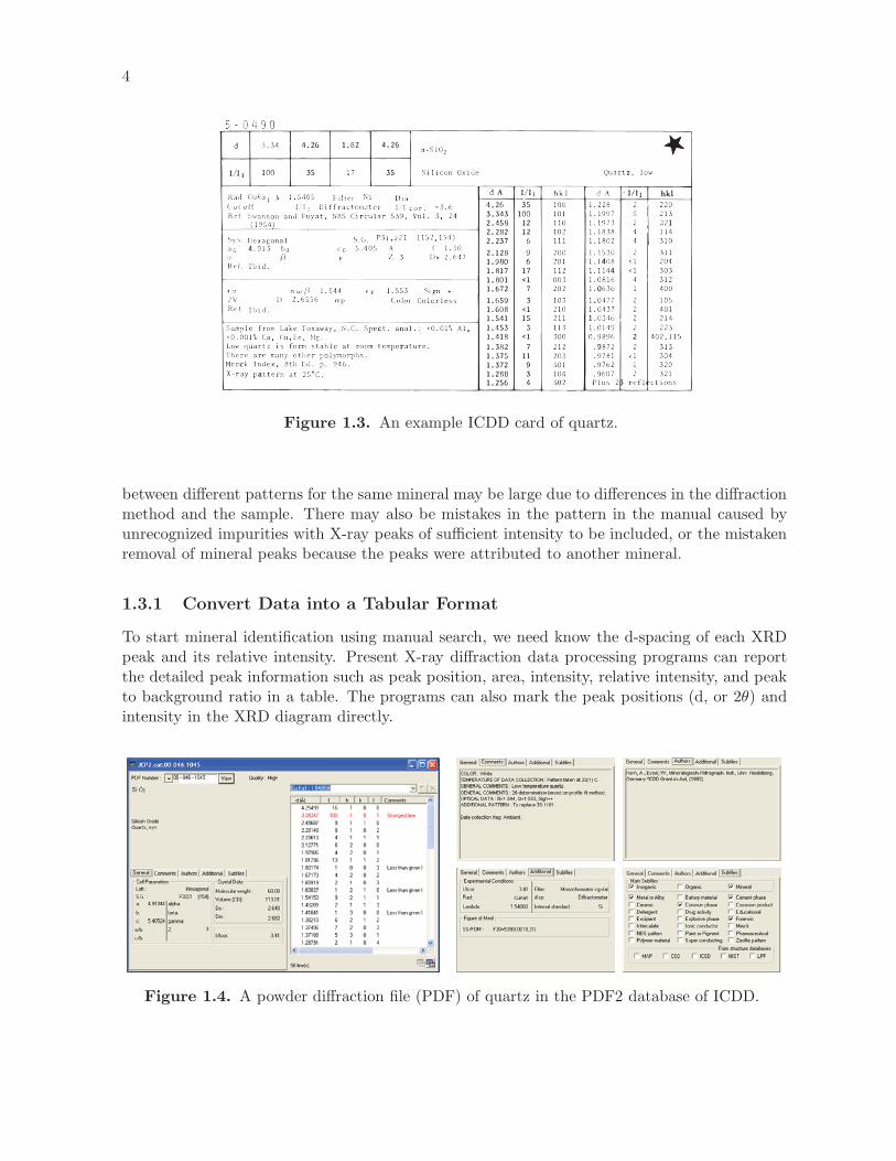
To start mineral identification using manual search, we need know the d-spacing of each XRDpeak and its relative intensity. Present X-ray diffraction data processing programs can reportthe detailed peak information such as peak position, area, intensity, relative intensity, and peakto background ratio in a table. The programs can also mark the peak positions (d, or 2θ) andintensity in the XRD diagram directly.
Figure 1.4. A powder diffraction file (PDF) of quartz in the PDF2 database of ICDD.
5
The first step in the use of the manual is to convert your data into a format similar to thatin the manual. To do this, you first make a table with the measured d-spacings and relativeintensities (scaled such the intensity of the tallest peak equals 100) for comparison to the searchmanual. Your raw data will be in a table containing a list of 2-theta values and counts forthat 2-theta. The file can be imported into Microsoft Excel. The two-theta values can beconverted into d-spacings using Bragg’s Law. Remember when calculating d-spacings from two-theta values that you need to divide the two-theta value by 2 to convert to theta. The point ona peak with the highest intensity (most counts) is usually considered the peak location. Thereare two methods that can be used to determine the peak intensities. The easiest is to use thenumber of counts at the tallest point in the peak less an estimate of the number of count for thebackground. Another method, which is more accurate for broad peaks, is to sum the number ofcounts above background for the peak.
It must be remembered that the unknown pattern may be a mixture of two or more mineralsand therefore, you must be prepared to use more than one combination of peaks in an attempt toidentify the unknowns in your sample. Also, it must be remembered that the relative intensitiesyou obtain from your Xray diffraction pattern may not exactly match those in the search manual.This is because the radiation source, particle orientation, and the diffraction technique affectthe relative intensities of XRD peaks. A mineral XRD pattern obtained using Mn filtered Fe Kαradiation and a powder camera will differ in intensities from a pattern obtained using graphitemonochromated Cu Kα radiation in a diffractometer with a theta-compensating slit. There arealso a few patterns with peaks that should not have been included in the ICDD book becauseof having an undetected contaminant or other errors. Always remember that any informationyou have on your sample (e.g. weathering environment, color, chemical composition) may helpin the sorting out of minerals whose X-ray diffraction patterns are close to the pattern for oneof the unknown minerals in your sample. Do not identify a mineral on the basis of a few XRDpeaks if it has characteristics (chemical composition, solubility, weatherability, etc.) that renderit unlikely in the sample. For example, a bulk sample from a surface soil that has been leachedby high amounts of rainfall for many years will probably not contain a soluble mineral withunusual elemental composition for its most common mineral.
1.3.2 Mineral Search Manuals
There are four sections in the early editions of the search manual: chemical index, Hanawaltindex, Fink index, and mineral name. Recently-published search manuals include more searchoptions e.g., cell length ratios, but they appeared to be less useful for identification of mixedmineral phases such as those in soil, sediments, or dust samples. Each section of the search man-ual sorts the XRD data in a different manner to increase the likelihood of mineral identification.For some samples, one method may have advantages over the others. You should always keepin mind the d-spacing range in your XRD pattern when looking in the search manual. Often,peaks are found in the search manual that could not be observed with your pattern becauseyour pattern did not include the same range in d-values as the pattern in the search manual.
1.3.2.1 Chemical Index
The first search method in the manual is by chemical name. In this section, minerals arearranged in alphabetical order depending on the chemical constituents of the mineral. This
6
section is useful for searching for the identity of a mineral in those cases where the chemicalmakeup of the mineral is known. If you know the chemical constituents, you search throughthis section to find that makeup and then compare your three strongest peaks with those shownuntil you get a match. Note that you can search for a chemical using any of its constituents.For example, if you are looking for a K−Fe−SO4−OH (the mineral jarosite, KFe3(SO4)2(OH)6),you could find it in four places:
• Hydroxide: Potassium Iron Sulfate
• Iron Sulfate Hydroxide: Potassium
• Potassium Iron Sulfate Hydroxide
• Sulfate Hydroxide: Potassium Iron.
1.3.2.2 Hanawalt Index
The second search manual section is the Hanawalt Index. The Hanawalt section is arranged onthe basis of the three strongest X-ray peaks. The first step to using this method is to arrangeyour X-ray spacings in order of decreasing relative intensities with the most intense first. Startthe search by finding the section of the manual that includes the d-spacing range with thespacing for the strongest peak. Use the second strongest reflection to further refine your choices.If this is unsuccessful and you have other peaks nearly as intense, try these peaks as the secondstrongest peak for the search. When you get a match for the first three, check to see whetherthe other peaks are correct and then look up the ICDD card to confirm any peaks beyond theseven most intense. Remember that your relative peak intensities are not necessarily the same asin the files. If the search is unsuccessful using the strongest peak that you observed, start againusing another strong peak.
1.3.2.3 Fink Index
The third search manual section is the Fink Index. The Fink Index is arranged based on thestrongest peak with the remaining peaks arranged with in order of decreasing d-spacing afterthe strongest peak. If you do not get a match for the strongest peak in this or the Hanawaltsearch method, choose a new peak to represent the strongest peak and start again. This sectionis especially useful for minerals that have one or more peaks occurring in the region above 10 A.
1.3.2.4 Mineral Name
The last index in the manual is arranged in alphabetical order by mineral name. This index isuseful if you know that certain minerals are present in a sample. You can then mark the peaksbelonging to the known minerals so you will know what peaks are from an unknown mineral.Marking the peaks of minerals that you know are present will reduce the number of unknownpeaks, lessening the confusion. Very rarely will you be asked to interpret an XRD patternwhere you have no knowledge about the sample. In most cases, with experience, you will beginto recognize the minerals you most commonly observe, such as quartz. Remember that, justbecause a mineral you know is in the sample has a peak at a certain location, the peak youobserve may also have a contribution from some other mineral. In that case, the peak intensitywill be a sum of the intensities from both minerals. Peak overlap is a major cause of errors inXRD patterns in the ICDD files.
7
0
1
2
3
4
5
0 20 40 60 80 100
0
0.01
0.02
0.03
0.04
0.05
0 20 40 60 80 100
2-Theta (degrees)
d-er
ror (
Ang
stro
m)
0.2o error
0.1 o error0.2
o error
0.1 o error
0
2
4
6
8
10
0 20 40 60 80 100
Rel
ativ
e d-
erro
r (%
)
0.2o error0.1 o error
2-Theta (degrees)
Absolute error Relative error
Figure 1.5. Absolute and relative errors introduced into determination of d-spacing froman X-ray diffraction when an error in measurement of the peak position in degrees 2θis 0.1◦ and 0.2◦ respectively.
1.3.3 Examples
To illustrate the use of the manual, three actual X-ray patterns are presented for practice inmineral identification using the manual. The first two are pure minerals and the third is amixture of two minerals. It must be remembered that these examples are actual patterns andnot perfect cases. If you cannot find a match with the strongest peak you should not hesitateto start a new search with the second or third strongest peak because the peak intensities maybe the result of preferred particle orientation.
Remember that differences in grain packing (how random is your packing compared to theone used for the ICDD pattern), X-ray source used, or types of diffraction (powder cameraversus X-ray powder diffractometer or theta compensating slits versus fixed slits) may resultin differences in relative intensities for the peaks from a mineral. When looking for a mineralmatching the one in your XRD pattern, you must also remember that the peaks may differslightly in position from that in the peak listings due to your (or their) choice for the peaklocation or slight goniometer misalignments. This is especially true for peaks at low 2θ. This isillustrated in Fig. 1.5. In this figure, the errors caused by an error in measurement of 0.1 and0.2◦ 2θ are shown as a function of 2θ for CuKα radiation. As you can see from Fig. 1.5a, ameasurement error of 0.2◦ 2θ for a peak at 8◦ 2θ (11.05 A) is 0.27 A while the error decreasesto less than 0.1 A for the same error at 20◦ 2θ. If one looks at the same error at 40 and 65◦
2θ (2.25 and 1.43 A, respectively) using Fig. 1.5, one sees the result of the error to be 0.01 and0.004 A. Therefore, most researchers use the lower d-valued XRD peaks for refining unit celldimensions and crystal structures. Similar data is available for other types of XRD collectiondevices.
8
Figure 1.6. X-ray diffraction curve for the first unknown mineral.
Example 1 Table 1.1 and the accompanying Fig. 1.6 contain a relatively simple X-ray patterncarried out to 65◦ 2θ using graphite monochromated Cu Kα radiation. The 2θ values in degrees,d-spacings in A, peak heights in counts per second, and relative intensities are contained inTable 1.1. The mineral present in this sample can be readily identified as there are at least 5versions of the mineral in the search index varying in chemical content. The identification isslightly hampered by the lack of what is commonly identified as the third strongest peak due tooverlap with the strongest peak. The peak at 2.796 A is the strongest peak and should be usedas the basis for the search. The next strongest observed peak is at 2.699 A with three otherpeaks (1.838, 2.629, and 3.454 A) more or less tied for the third strongest. Start the search bygoing to the 2.79 - 2.75 A part of the Hanawalt section of the search manual. Then, look downthe second column until you get to 2.72 - 2.68 A. You become confused at this point as there areseveral minerals in that region that have several peaks that appear on the XRD pattern. If youlook closely you will notice that three of them are very similar. Each of these minerals has allthe peaks listed except one at about 2.80 - 2.81 A which overlaps with the strongest peak. Thedifferences between these three minerals (9-432, 15-876, and 19-272) are very small differing insubstitution in one site. This is the mineral that made the XRD pattern, apatite. To verify theidentification, check diffraction peak position and intensity against the ones listed in the ICDDfile book.
9
Table 1.1. Peak locations and heights for the unknown mineral in the X-ray diffractionpattern shown in Fig. 1.6.
Figure 1.7. X-ray diffraction pattern for the second unknown mineral.
Example 2 The X-ray pattern for the second mineral has many more peaks in the regioncovered (Table 1.2 with Fig. 1.7) than the previous example and so a mixture is suggested. Inthe search of the manual, first start by looking in the region that includes 3.05 A for secondarilystrong peaks at 7.54 and 4.26 A. Examination of the manual in the region 3.09-3.05 A revealsthat the mineral, gypsum has its strongest peak at 3.066 A with strong secondary peaks at 4.27and 7.56 A. Comparing the manual to the pattern further, it becomes evident that the measuredpattern has peaks that agree with all 8 peaks in the search manual and therefore confirms thepresence of gypsum (CaSO4 · 2H2O). To determine whether the other 11 peaks also result fromgypsum, look up ICDD card 6-46 for comparison. It is evident that all the remaining peaks arepossible gypsum peaks and so a relatively pure gypsum sample is indicated.
11
Table 1.2. Peak locations and heights for the unknown mineral in the X-ray patternshown in Fig. 1.7. Note that the first two peaks chosen by the computer are not real.
Figure 1.8. X-ray diffraction curve for a mixture of unknown minerals.
Example 3 Example 3 (Table 1.3 with Fig. 1.8) is an example of an X-ray diffraction patterncontaining two common soil minerals. The first step is to decide on which peaks to use in thesearch. In this case, choose the 4 strongest peaks (all have relative intensities of more than 50%of the tallest peak) assuming that one mineral will have at least 2 of these peaks in its strongest3 peaks and would therefore be determined with little problem with the search manual. Firstnote that there is no good match for any of the minerals with the strongest (3.34 A) peak andthat therefore the remaining peaks are the result of another mineral or minerals. No good matchwas found using the 2.68 and 2.51 A peaks. Yet the 2.69 and 1.69 A peaks match hematite andthe 2.51 A peak also corresponds with a hematite peak as do the weaker peaks at 3.658, 2.199,1.836, 1.484, and 1.452 A. Looking up the ICDD card for the mineral, it is evident that the2.282, 1.633, and 1.597 A peaks were also the result for hematite. After marking these peaksout of the search, a match for quartz with the 3.34 and 4.25 A peaks is found. Examination ofthe ICDD card for quartz reveals the remainder of the peaks in the X-ray diffraction patternexcept the 2.236 A peak, which is very weak (relative intensity of 7). Thus this pattern is aresult of a mixture of quartz and hematite and a trace of an unidentified mineral.
13
Table 1.3. Peak locations and intensities for the X-ray diffraction pattern of the unknownmixture. Note first 3 peaks chosen by the computer are not real. The actual patternwith labeled corresponding to the table is in Fig. 1.8.
1.4 Other strategies for mineral identification based on XRD
1.4.1 Using web-based mineralogy databases
Several web-based mineralogy databases, e.g., MINCRYST (http://database.iem.ac.ru/mincryst)and the American Mineralogist Crystal Structure Database (http://www.minsocam.org/MSA/Crystal Database.html) offer diffraction peak positions of minerals. Some of them list the threestrongest peaks for mineral identification. One example web site with this capability is the web-Mineals (http://www.webmineral.com). Part of a screen shot of the web site is given in Fig. 1.9.You can check the strongest peaks of an unknown sample against the list and to find the bestmatch.
Listing of 6122 Records Sorted by D1 using 1.54056 - CuKa1 for 2θ
Figure 1.9. Part of a screen shot of the webMineral page showing a list of d-values andintensities of the three strongest peaks.
1.4.2 Comparing a recorded XRD pattern to those of reference minerals
Several free softwares for quantitative mineral analysis come with XRD patterns of referenceminerals. One can check the pattern of an unknown sample against those of the standards andto find the best match. For example, program RockJock by Eberl (2003) has more than 100XRD patterns in its library (Fig. 1.10), FullPat by Chipera and Bish (2002) has also about 25XRD patterns of common minerals. Those programs can be downloaded from the web site ofthe Collaborative Computational Project No. 14 (CCP 14) at http://www.ccp14.ac.uk. Onecan also build his/her own standard library either by theoretical calculation or recording realsamples. Studying the XRD patterns of these reference minerals will greatly shorten the timeand increase the accuracy in mineral identification.
One can import the XRD patterns of standard minerals and the unknown sample into thesame spread sheet in Excel and compare them side by side as shown in Fig. 1.11. Scaling thestandard patterns to the same peak heights can offer some estimation of the mineral composition.For a more accurate quantification, one can use the full function of the programs. One need be
15
Figure 1.10. The X-ray diffraction data library in program RockJock by Dennis D.Eberl.
cautious about the quantitative analysis since the standards in those programs were recordedon specific X-ray diffractometers, which may have different configurations and/or operatingconditions from the system with which the unknown sample is recorded.
2-Theta (degree)
0
500
1000
1500
2000
2500
2 10 20 30 40 50 60
d=10
.031
24 d=4.
4836
6d=
4.26
338
d=4.
0544
4d=
3.85
470
d=3.
7700
2
d=3.
343
d=3.
2186
2d=
3.03
526
d=2.
6160
0d=
2.59
440
d=2.
5665
5d=
2.49
010
d=2.
4606
5
d=2.
2830
9d=
2.23
771
d=2.
1767
1d=
2.12
772
d=2.
0914
8
d=1.
9941
2d=
1.98
162
d=1.
9255
0d=
1.91
159
d=1.
8746
7d=
1.82
005
d=1.
7973
9
d=1.
6731
2
d=1.
6024
2
d=1.
5434
5
d=1.
5002
6
d=1.
4551
2d=
1.43
797
Quartz
CalciteKaolinite
Musovite (2M1)
Ordered microcline
Inte
nsity
(Cou
nt/s
econ
d)
Figure 1.11. Comparing a recorded XRD pattern to those reported in program ROCK-JOCK (Eberl, 2003).
16
Chapter 2
Sample Evaluation
2.1 Introduction
The primary goals of mineralogy analyses are (1) to identify mineral species, (2) to quantifymineral composition, and (3) to reveal mineral structures that determine the chemical reac-tivity of the minerals. Many techniques can be used for mineralogy analysis, such as pet-rographic microscopy, scanning electron microscopy (SEM), transmission electron microscopy(TEM), X-ray diffraction (XRD), electron diffraction, neutron diffraction, Fourier transforminfrared spectroscopy (FTIR), Raman spectroscopy, nuclear magnetic resonance (NMR), elec-tron paramagnetic resonance (EPR), Mossbauer spectroscopy, chemical analysis, computationalmodeling, and many more. Each technique has its own merits and drawbacks. One techniquemay not be equally suitable for different samples or for different fractions of one particular sam-ple. Among these techniques, we are going to use XRD, SEM, TEM, FTIR, chemical analysis,and computational modeling for most soil, sediments, and dust samples.
Natural samples, such soils, sediments, and dusts, are often mixtures of minerals, short-distance ordered phases (amorphous), organic matters, and biological organisms. Ideally, min-eralogy analysis should be performed on undisturbed samples without any treatments to revealthe real mineral composition and structure in situ. Practically, soil samples have to go throughsome treatments, such as removing cementing and flocculating compounds (organic matter,carbonate, and/or soluble salts), size fractionation, cation saturation, solvation, and heating.Otherwise, only limited information can be obtained from an analysis. The major reason forthese treatments is to concentrate some minerals in certain fractions and therefore, to enhancethe signals of the species interested. Segregation of the minerals either by size, gravity, mag-netic property greatly simplify the subsample composition and therefore, reduce the ambiguityin mineral identification and quantification.
Figure (2.1) is a flow chart of mineral analysis performed in our lab. We select thesetreatments to maximize the efficiency of mineral separation and to minimize mineral structuralalteration during the treatments. Three important procedures for sample treatments are:
1. Preliminary check of oxidizing/reducing compounds (organic matter, sulfide, and man-ganese oxides), carbonate minerals, and evaporates (gypsum, soluble salts). These com-pounds will be removed from samples by pH 5 sodium acetate [CH3COONa], hydrogenperoxide (H2O2), and dispersion solution. For samples containing significant amounts ofthese phases, additional analyses should be performed to quantify them if the primary goal
17
Chapter 3
Removal of Flocculating andCementing Materials
Removal of flocculating and cementing materials from samples enhances the dispersion of in-dividual soil particles, and therefore, facilitate size fractionation. Flocculating materials aresoluble salts and polyvalent cations that are adsorbed on soil particles. Cementing agents arecarbonate minerals of alkaline-earth elements (Ca 2+ and Mg 2+), organic matter, oxides andhydroxides of iron, amorphous silica and alumina (Whittig and Allardice, 1986). In this lab, weremove carbonates with a pH 5 sodium acetate buffer solution and remove organic matter withhydrogen peroxide. During these treatments, soluble salts are removed by the solutions. ThepH 5 sodium acetate buffer solution replaces Ca and Mg cations at the exchange sites as well.
3.1 Removal of carbonate minerals
3.1.1 Principle
Carbonate minerals can be destroyed by acid through the following reactions:
CaCO3 (calcite) + 2 H+ = Ca 2+ + CO2 ↑ + H2O (3.1)
MgCa(CO3)2 (dolomite) + 4 H+ = Ca 2+ + Mg 2+ + 2 CO2 ↑ + 2H2O (3.2)
Dolomite reacts with acid more slowly than calcite does. Heating is required to speed thedestruction of dolomite. A pH 5 sodium acetate buffer solution is used as the acid source. Thisbuffer is used to avoid significant dissolution of other minerals in the sample. The pH of thesodium acetate buffer is set near to the pKa of 4.7 for acetic acid [CH3COOH] so that a largeamount of acid or base is needed to cause a significant change in pH. Due to the low activity ofH+ (10−5) in the buffer, the destruction rate of carbonate minerals in the buffer is much slowerthan that in a strong acid e.g., 1 M HCl. Temperature is raised to increase the reaction rate.
3.1.2 Reagents
• Sodium acetate trihydrate [CH3COONa · 3 H2O]
• Glacial acetic acid [CH3COOH]
33
Chapter 4
Soil Mineralogy Field Trip
4.1 Introduction
During a half-day local field trip to the Range Science area (Fig. 4.1) near the Eastwood Airport,College Station, Texas, we will have the opportunity to study 20 minerals as they occur inthe natural environment. Some of the minerals are residual (e.g. mica, quartz) and othersare authigenic (e.g. gypsum, jarosite and some of the silicate clays). By obtaining visualimages of these minerals as they occur in soils and sediments, we can identify them and inferthe conditions that led to their occurrence and to infer the soil formation processes. We willestablish some easily recognized properties of these common minerals that will mesh with themore abstract analytical properties that are required for positive identification of minerals insoils and sediments. This is also an excellent opportunity to use the knowledge learned in theclass to explain the geochemical processes and solve environmental problems in the real world.
Preparation for the field trip: Develop a 5-minute presentation on the mineral or groupof minerals that you are assigned. Be prepared to give this brief description in the field atthe site where the mineral(s) occur. Study the information below and your text to prepare thepresentation. Be prepared to answer questions on the mineral(s) you are assigned. Presentationsmay include: structure, formation, physical and chemical properties and importance and use.
Conventions used in the following mineral description The 20 minerals represent severalimportant mineral groups (i.e. sulfates, carbonates, oxides, phyllosilicates, and tectosilicates) insoils and sediments. In the following description of the minerals, each group of the minerals iscoded with a number shown in the table below:
Group Number Minerals1 Carbonates2 Sulfides3 Sulfates4 Oxides5 Phyllosilicates6 Tectosilicates
In the formula of the minerals, symbol “X” is used to stand for exchangeable cations in theinterlayer space or tunnels of minerals.
39
Chapter 5
Size Fractionation
After removing flocculating and cementing agents, the sample is ready for size fractionation.It is washed with deionized water to remove the residual chemicals (e.g., pH 5 NaOAc buffersolution and H2O2), and then suspended in a diluted pH 10 Na2CO3 solution. The sand particlesare separated by sieving; silt and clay fractions are separated by centrifugation or sedimentationbased on Stokes’ Law (Section 5.5).
5.1 Sample Dispersion
5.1.1 Principle
Minerals in the clay fractions have either permanent charges due to isomorphous substitutionor variable charges (pH-dependent). Phyllosilicate minerals have permanent negative chargeson basal surfaces and variable charges on the edges of the layers. By raising pH, the variable-charge surfaces, e.g., the surfaces of iron oxides and hydroxides, and edges of phyllosilicatesbecome negatively charged. The electrostatic repulsion among the negatively charged particlesenhances the dispersion of the particles in solution. Reducing electrolyte concentration ofthe solution increases the double-layer thickness of the colloids and facilitates the dispersion.Monovalent cations can induce thicker double-layers on the colloid surfaces than polyvalentcations. For these three reasons, a diluted sodium carbonate (0.125 g L−1 Na2CO3, aboutpH 10-10.5) is used as the dispersion agent.
5.1.2 Reagent
• Sodium carbonate [Na2CO3] solution, about pH 10: 0.125 g L−1. Large quantity of thissolution is used as the dispersion agent. Make 20 L each time.
5.1.3 Procedure
a. Add about 50 mL pH 10 sodium carbonate dispersion agent to the sample in which floccu-lating and cementing materials have been removed. Cap the bottle and shake it to suspendsoil/sediment particles.
b. Centrifuge the bottle at 2000 rpm for 10 min. If the supernatant is cloudy, proceedto Separation of the Sand Fraction (Section 5.2). Otherwise, pipet or siphon off the
51
Chapter 6
Sample Preparation for X-rayDiffraction and Interpretation ofXRD Patterns
6.1 Sample preparation for X-ray diffraction analysis
For X-ray diffraction (XRD) analysis, an important procedure is to homogenize the sample sothat the collected XRD pattern is representative. Usually, randomly-oriented powders are usedin the XRD analysis for sands and silts, for which orientation preference of the particles shouldbe minimized. The sand particles are ground to minimize the orientation preference and tomaximize sample representativeness.
The sand fraction requires grinding to a size less than 140 mesh to prepare it for XRD.
6.1.1.1 Procedure
a. Grind a representative sample of the sand fraction. The silt fraction is by definitionsmaller than 140-mesh and is therefore already prepared for X-ray diffraction if dried atoven temperatures (110 ◦C). Do not grind a larger sample than is needed to fill the XRDpowder holder.
b. Front load a subsample of each fraction into a labeled powder holder (See Fig. 2.5).
c. Leave the prepared sample where it is obvious for the instructor to find. It will be X-rayedfrom 2◦ to 70◦ 2-theta using Cu Kα radiation. The range of 2◦ to 70◦ degrees 2-theta waschosen to provide enough X-ray diffraction peaks to identify most common soil minerals.
67
Chapter 7
X-ray Diffraction of Minerals
An introduction to diffraction condition, production and properties of X-rays, and the major X-ray optic components is necessary for successful applications of the X-ray diffraction techniques.We need emphasize that safety and protection are important when one is working with X-rays.The X-ray radiation itself and the high voltages used to generate X-rays make the usage ofX-ray diffraction equipment potentially hazardous. It is especially important for workers to notexpose themselves to X-ray radiation as the effects of exposure are cumulative and may lead topermanent injury. Fortunately, modern X-ray diffractometers have safety features that preventalmost all accidental exposures to X-ray radiation.
7.1 Theory of X-ray diffraction
7.1.1 Bragg’s Law
The fundamental physics of X-ray diffraction is the same as the diffraction by other electromag-netic radiations that we are familiar with. For example, the brilliant colors on soap bubbles arethe result of diffraction of visible light. Diffraction occurs where the interferences of individualradiations are constructive. When X-ray diffraction occurs, all coherently scattered X-rays fromthe (hkl) planes must be in phase (Fig. 7.1, upper part).
We only consider the phase relationship from two adjacent (hkl) planes (Fig. 7.1, lowerpart). When X-rays leave the X-ray source, all incident wavelets are in phase. The X-ray fromthe second plane travels a longer distance than that from the first plane. The path lengthdifference between the two reflections is
AP + PB = d sin θ + d sin θ = 2d sin θ. (7.1)
To have the scattered X-rays in phase, the path difference of the two X-rays from the adjacentreflections must be an integer number of the wavelength λ of the X-ray.
nλ = 2d sin θ (7.2)
When they are in phase, the phase difference between the two radiations from adjacent (hkl)planes is n2π. Another condition for the occurrence of X-ray diffraction is the incident angleand diffracted angle must be equal to each other.
θincident = θdiffracted (7.3)
87
Chapter 8
Simulating One-dimensional XRDPatterns with NEWMOD
8.1 Introduction
NEWMOD is a program that calculates one-dimensional XRD patterns for phyllosilicates. Asstated on the web site of the software, “NEWMOD is an integrated package for calculatingdiffraction patterns for mixed-layered clay minerals, mixing calculated patterns to simulatenatural samples for quantitative analysis, plotting patterns to different scales, measuring andlabelling d, 2θ, integrated areas, and peak widths at half maximum height”1.
A one-dimensional pattern is what is obtained when oriented clay slides are X-rayed. Theprogram will calculate theoretical patterns for pure clay minerals and for interstratificationsof any two phyllosilicates. You can also use this program to add together XRD patterns thathave been saved earlier to simulate observed patterns. An introductory description about thevariables in NEWMOD can be found in the article of Walker (1993). Thorough treatment aboutthe theory behind the program can be found in a series of publications of Reynolds, Jr., theauthor of the program, e.g., Reynolds (1980), Reynolds (1989), and Reynolds and Walker (1993).
Variables used in the calculation of the patterns are of two main types. One group of vari-ables includes the diffractometer parameters including the slit sizes, whether or not you use atheta compensating slit, etc. These can be preset to values that are used by the diffractome-ter producing the observed patterns so that the calculated patterns are consistent with thoseobserved. The second group of variables include mineral specific parameters such as octahe-dral cation occupancy, thickness and defect ordering of the individual diffracting domains, theobserved d-spacings for the minerals, and in chlorite, the fractional filling of the hydroxyl inter-layer. Proper use of these variables allow for the calculation of patterns for the minerals thatare similar in diffraction characteristics to those observed in actual X-ray patterns. You candetermine the amount of octahedral Fe, and use the defect broadening and thickness param-eters to produce a calculated pattern with XRD peak widths that are as close as possible tothose observed. A file mixing program is included that allows you to add calculated patternsof individual minerals together to simulate a pattern for a sample which contains a mixture ofminerals.
In the past, we have used NEWMOD 1.1, a DOS version of the program. We now have
1Accessed in December 2007: http://www.angelfire.com/md/newmod/
The essence of mineralogy lies in the subtle chemical substitutions that divide one mineralspecies from another. X-ray diffraction is largely concerned with long-range order or periodicityin crystals. Differences are measured on the unit cell level. Substitutions in the crystal structurecan be detected in two ways. If the substitution results in changes in unit cell size, peak shiftswill signal a change in the mineral. Substitutions may also be detected by changes in the relativeintensities of the peaks on the XRD pattern. The exact nature of the changes in the mineralcannot always be determined by direct examination of the XRD pattern. Detection of smallerscale differences such as ionic substitutions requires extensive mathematical processing of XRDdata to determine the minerals crystal structure.
Infrared analysis, on the other hand, is concerned with the fine structure (e.g. chemicalbonds), between nearest neighboring atoms. As only the nearest neighbors are important,the symmetry of the individual tetrahedra and octahedra are more important. A distortedpolyhedron will have a more complex infrared pattern than an ideal polyhedron. An absorptionband in an infrared spectrum will tell the chemistry of individual polyhedra but yields littleinformation on the identity of the mineral containing the polyhedra. Thus, infrared spectroscopyis complementary to XRD analysis, each resulting in data ancillary to the other. Infraredspectroscopy is even more important for the study of adsorbed molecules on soil particles.
Light is a collection of frequencies in the electromagnetic spectrum. Radiation of differentenergy levels has markedly different effects upon the atomic and molecular associations (Fig. 9.1).Ultraviolet light with wavelengths between 50000 and 25000 cm−1 has higher energy and issensitive to electron shifting. Visible light, 25000-14286 cm−1, is likewise sensitive to electronshifts. This is why ferric Fe is red while ferrous Fe is not. Infrared spectroscopy is concerned withthat region of the electromagnetic spectrum extending from the red end of the visible spectrum(about 14000 cm−1) to the microwave region (20 cm−1). Electromagnetic radiation in theinfrared region is capable of causing the changes of bending, twisting, rotating, and stretchingvibrations in the bonds present in minerals and other compounds because the frequency ofoscillation of atoms and molecules about their equilibrium position is in the same range as theinfrared radiation. When a sample is placed in an infrared beam, the infrared beam distorts the
115
Chapter 10
Scanning Electron Microscopy
10.1 Introduction
According to Bozzola and Russell (1992), electron microscopy is “a specialized field of sciencethat employs electron microscope as a tool”. The scanning electron microscope (SEM) and thetransmission electron microscope (TEM) were conceived almost simultaneously, the developmentof the SEM lagged considerably behind that of the TEM. Their uses are fundamentally different.
The method used for specimen magnification in SEM differs considerably from that usedin optic microscope and TEM (Fig. 10.1). In optic microscope, a condensed light beam passesthrough a specimen, is refracted by sets of objective and projector optical lenses and focused tobe seen by naked eye or to be recorded by a camera. The optical system in a TEM works in asimilar way as in an optic microscope. In TEM, a condensed electron beam passes through a thinspecimen, and is focused by objective and projector electromagnetic lenses such that a magnifiedtwo-dimensional image is formed on a phosphorescent screen. In SEM, a highly focused electronbeam (2 to 3 nm spot size) scans the surface of the specimen, interaction of this beam withthe surface results in the formation of several types of signals (Fig. 10.2), including secondaryelectrons, backscattered electrons, Auger electrons, characteristic X-rays, cathodoluminescence,and transmitted electrons. Depending on the availability of detectors in an electron microscope,several types of signals can be recorded. For most morphological observation, the secondaryelectron signal is collected, and converted to electron pulses, which are then used to reconstructthe image on a cathode ray tube (CRT) spot by spot (Goldstein and Yakowitz, 1975), yieldingan image that gives impression of three dimensions. The signals can also be recorded and storedin a computer and processed separately. In addition to morphology, chemical composition andcrystal structural information can be collected with both SEM and TEM.
The high magnification power of electron microscopes is certainly one of the major attractivefeatures of the instruments, but bear in mind, it also means only limited samples are analyzedby the microscope. Williams and Carter (1996) described the electron microscopes as “terriblesampling tools”, and state only less than 0.6 mm3 materials had been examined by all TEMssince they were first became available commercially. It is critical to know your sample by othermeans, such as X-ray diffraction, optic microscopy, analysis of physical and chemical propertiesbefore you load it in an electron microscope.
133
Chapter 11
Transmission Electron Microscopy
11.1 Introduction
Transmission electron microscopy (TEM) has several unique properties that make it a verystrong method to add to the selection that you have already been introduced to in this course1.The TEM permits morphology viewing, chemically analyzing (EDS), and structurally analyzing(electron diffraction) sub-micron particles. Although the data may not be quantitative theybring together a powerful set of observations at the instrument that are particularly importantfor analyzing mixed systems like soils. Also, you will use them at a crucial time in your learningprocess about the properties of individual minerals. These data will help you to integrate thevarious properties with a visual image of each particle. Thus it is important to know what themajor minerals are in your sample by studying the x-ray diffraction data before you go to theMicroscopy and Imaging Center to study your samples. Only TEM will answer at the instrumentsuch questions as -do certain particles contain plant nutrients, is a particle a single crystal, doesit have randomly stacked layers, or is it amorphous.
In 1924, de Broglie (1929 Nobel Laureate in Physics) showed that electrons havewave properties even though they are particulate in nature. The focusing ofelectrons by magnetic lenses is analogous to the focusing of light by glass lenses(Fig. 11.1a). Electrons have a much shorter wavelength (at 200 kV, 0.0025 nm)than visible light (400 to 700 nm) or X-rays (Cu Kα, 0.154 nm). As illustratedlater, electrons are diffracted in an analogous way to X-rays but at much smallerangles. It is the short waves that permit us to “see” small objects such as clayparticles by TEM.
The TEM sessions are intended to present data of four types: morphology, selected areaelectron diffraction (SAED), lattice fringes (all three are illustrated in Fig. 11.2) and moire fringes(Fig. 11.3). The latter three types of data are structural. The SAED of platy particles orientedparallel to the mounting grid give information on the a-b plane of the mineral (Fig. 11.1b)which is largely unavailable from the X-ray diffraction (XRD) patterns of clay aggregates withpreferred orientation of particles (Fig. 11.1c). Thus, TEM data complement the XRD data. Aset of parallel moire fringes is produced when two crystals overlap but at a slightly differentangle. Fig. 11.3 illustrates several sets of moire fringes.
1A PowerPoint presentation of the transmission electron microscope JEOL 2010 prepared by J. B. Dixon isavailable on the departmental website. It is intended to prepare you for the lab exercise for study of your sample.
153
Chapter 12
Quantification of Free Iron (Fe)Oxides
Iron oxides sometimes act as cementing agents of aluminosilicates and cause difficulty in soildispersion. The removal of Fe oxides aids in dispersion of the silicate portion, which may benecessary for effective segregation of the colloidal aluminosilicates present. The removal of Feoxides concentrates the silicates, and enhances the degree of parallel orientation of the silicatelayers with a consequent increase in basal diffraction intensity. The removal of coatings from thesilt and sand particles aids in their identification by means of the polarizing microscope. In theSoil Mineralogy Laboratory at Texas A&M, iron oxides are not removed prior to fractionationto allow for the determination of which Fe oxides are present by XRD and TEM methods andexamine their properties. Iron oxides can be removed by chemical or physical (magnetic) means(Schulze and Dixon, 1979). For quantitative removal, chemical removal is required. Manymethods have been applied to the selective determination of the oxide bound Fe. The two mostcommonly applied selective dissolution techniques use either a combination of Na dithionite,Na citrate, and Na bicarbonate (DCB) or ammonium oxalate and fluorescent light. The twotechniques work equally well for the oxides. Each has undergone many modifications during theperiod since their introduction.
The technique used in class for the removal of iron oxides is the sodium dithionite-citrate-bicarbonate procedure of Mehra and Jackson (1960). Sodium dithionite [Na2S2O4)] reducesferric iron (Fe 3+) to ferrous iron (Fe 2+) in solution, causing the iron oxide (and any otheroxidized material in the sample) to become more soluble:
The sodium citrate Na3[HOC(COO – )(CH2COO – )2] acts as a chelate to keep the reactionmoving towards the end result of dissolution of all Fe oxides by complexing the iron (ferrousand ferric) in solution.
[HOC(COO−)(CH2COO−)2]3− + Fe 2+ = [HOC(COO−)(CH2COO−)2Fe]− (12.4)
[HOC(COO−)(CH2COO−)2]3− + Fe 3+ = [HOC(COO−)(CH2COO−)2Fe] 0 (12.5)
165
Chapter 13
Cation Exchange Capacity (CEC)Determination
13.1 Introduction
Cation exchange capacity (CEC) is a measure of the quantity of readily exchangeable cationsneutralizing negative charge in the soil. The CEC, usually expressed in cmol(c) kg−1 of soiland formerly as milliequivalents per 100 g, differs from one clay mineral to the other. Thesedifferences will permit estimation of the relative proportions of the minerals in a sample.
Many methods have been used to determine the cation exchange capacity of a soil. A surveyof possible techniques for determining CEC can be found in Chapman (1965) and Sumner andMiller (1996). While the exact exchange capacity measured will vary from method to method,the relative magnitude of the exchange capacity will be the same except in those cases wherethere is some type of ion sieving or fixation. Some exchangeable cations are replaced more easilythan others with the completeness of the reaction depending upon the ions, pH, and solutionconcentrations of the cations (Chapman, 1965).
The objectives of this procedure are to determine the cation exchange capacity (CEC) andto estimate the amount of highly charged clay minerals in the clay samples. Note: The samplesmust be free of calcium carbonate before CEC determination. If not, dissolution may release Cain the displacing solution.
• 0.005 M CaCl2 - This is usually mixed by making a one hundred fold dilution of the 1 N(0.5 M) CaCl2 rather than weighing out the chemicals and adding the water.
• 0.5 M MgCl2 (101.65 g MgCl2.6 H2O /liter)
• Standard sample of a known CEC (Volclay N. 200 Montmorillonite).
169
Chapter 14
Quantification of Mica by Total KDetermination
14.1 Introduction
Mica in clay samples is often estimated using total K. The principal error from making suchan estimate is due to the presence of K-feldspars. If no K-feldspars are present determinationof total K will permit an estimate of mica content for samples that have no exchangeable K.It is important to replace any exchangeable K with another cation so the K present on theexchange complex does not interfere with the mica determination. If the samples contain noK-feldspar and is not K saturated, then the mica content can be estimated by assuming that10% K2Ois equivalent to 100% mica. This conversion factor is used as the K2O content for micasvary from 9.25% K2O in annite [Fe-biotite, KFe3(AlSi3)O10(OH)2] and 11.8% K2O in muscovite[KAl2(AlSi3)O10(OH)2].
Many methods have been applied to determine the total contents of various elements inminerals. The most common methods used are acid dissolution (see for instance Olson, 1965;Pratt, 1965; Bernas, 1968; Hossner, 1996; Helmke and Sparks, 1996) and fusion in either Na2CO3
(see for example Kanehiro and Sherman, 1965; Kilmer, 1965) or with a Li-borate salt. Mostof the acid dissolution methods use hydrofluoric acid (HF) with other acids. Hydrofluoric acid,although a relatively weak acid, is very effective in the dissolution of minerals because of thestrong complexes formed by the cations in the minerals with the F – ion. The HF method usedis a modification of the Bernas (1968) method. In the original form, the sample is digested atelevated temperatures in a digestion bomb. In the form used here, the solutions and sampleare measured directly into a Nalgene volumetric flask where the digestion is allowed to continueat room temperature. This version of the technique has the advantage of reducing potentialfor sample loss during transfer steps. The disadvantage of this technique is that some HF maybe lost along with Si and some other cations if the top of the volumetric is not sealed tightly.The aqua regia is diluted to increase the fluid volume during the reaction and to increase thestability of the aqua regia, which goes bad if too old.
Quantitative analysis is a rigorous process where exact quantities are measuredand contaminants are avoided by using clean apparatus, exact measurements, andconsistent procedures.
175
Chapter 15
Integrating Different Data forQuantification
15.1 Quantitative Analysis of Clays Using CEC, Total K, and
NEWMOD
At this point in the laboratory procedure, the minerals are known from the XRD patterns andyou have total K, FTIR and CEC results. It is possible to quantify the clay if two phyllosilicateclay minerals and mica (assuming no feldspars) are present. First, calculate the concentrationsof the minerals using simultaneous equations. Assuming the sample contains no non-crystallinematerial, the first equation results from the sum of the concentrations of the minerals equalingone. For instance, consider a clay sample that contains mica, kaolinite, and smectite. For thisexample:
1 = XM + XK + Xs (15.1)
where XM is the concentration of mica, XK is the concentration of kaolinite, and XS is the con-centration of smectite. As the total K results can be used to estimate mica using the assumptionof 10% K2O equals 100% mica, the equation reduces to two unknowns:
1−XM = XK + Xs (15.2)
with the (1-XM ) becoming a constant. The second equation results from the CEC data for thefraction. Assuming values for the CEC of the smectite, mica, and kaolinite to be 110, 10 and5 cmol/kg, respectively, the following equation is obtained:
CECsample = 10XM + 5XK + 110XS (15.3)
As the value for XM is known from the total K data, this equation can be reduced to twounknowns:
(CECsample − 10XM ) = 5XK + 110XS (15.4)
with the term (CECsample − 10XM ) being a constant. Now there are two equations with twounknowns:
American Geological Institute (1976). Dictionary of Geological terms. Anchor Books, GardenCity, New York.
Ball, D. W. (1994). The spectroscopist’s tools ii. fourier transform spectrometers. Spectroscopy,9(8):24–25.
Bernas, B. (1968). A new method for decomposition and comprehensive analysis of silicates byatomic absorption spectrometry. Anal. Chem., 39:1210–1216.
Berner, R. A. and Holdren Jr., G. R. (1979). Mechanism of feldspar weathering - II. Observationsof feldspars from soils. Geochimica Et Cosmochimica Acta, 43:1173–1186.
Besson, G. and Drits, V. A. (1993). Relationships between infrared spectra analysis and chemicalcomposition of dioctahedral micaceous minerals. In Abstract of the 10th International ClayConference, page 155, Adelaide, South Australia.
Beutelspacher, H. and van der Marel, H. W. (1968). Atlas of Electron Microscopy of ClayMinerals and their Admixtures. Elsevier Publishing Company, New York.
Bozzola, J. J. and Russell, L. D. (1992). Electron microscopy: principles and techniques forbiologists. Jones and Bartlett, Sudbury, Mass., 2nd edition.
Chapman, H. D. (1965). Cation-exchange capacity. In Black, C. A., editor, Methods of soilanalysis. Part 2. Chemical and microbiological properties. Agronomy 9 Madison, WI., pages891–904. American Society of Agronomy, Madison, WI.
Chipera, S. J. and Bish, D. L. (2002). FULLPAT: a full-pattern quantitative analysis programfor X-ray powder diffraction using measured and calculated patterns. Journal of AppliedCrystallography, 35(6):744–749.
Dixon, J. B. (1978). Electron microscopy studies. In Barnhisel, R. I., editor, Analyses ofClay, Silt and Sand Fractions of Selected Soils from Southeastern United States, SouthernCooperative Series Bulletin 219, pages 77–88. University of Kentucky, Lexington, KY.
Dixon, J. B. (1999). Instruction in HRTEM through the useful example of goethite in soils.In Kodama, H., editor, Proceedings of 11th International Clay Conference, pages 385–389,Ottawa, Canada.
Dixon, J. B. and Schulze, D. G., editors (2002). Soil mineralogy with environmental applications.Soil Science Society of America book series ; no. 7. Soil Science Society of America, Madison,Wis.
Dixon, J. B. and Weed, S. B. (1989). Minerals in soil environments. Soil Science Societyof America book series, No. 1. Soil Science Society of America, Madison, Wis., USA, 2ndedition.
Douglas, L. A. (1989). Vermiculites. In Dixon, J. B. and Weed, S. B., editors, Minerals in
183
184
soil environments, Soil Science Society of America book series, No. 1, pages 635–674. SoilScience Society of America, Madison, Wis., USA, 2nd edition.
Douglas, L. A. and Platt, D. W. (1977). Surface morphology of quartz and the age of soils. SoilScience Society of America Journal, 41:641–645.
Eberl, D. D. (2003). Users guide to ROCKJOCK – a program for determining quantitativemineralogy from powder X-ray diffraction data. Technical Report Open-File Report 03-78,U. S. Geological Survey.
Farmer, V. C. (1974a). The layer silicates. In Farmer, V. C., editor, The Infrared spectra ofminerals, pages 331–363. Mineralogical Society, London.
Farmer, V. C. (1974b). Vibrational spectroscopy in mineral chemistry. In Farmer, V. C., editor,The Infrared spectra of minerals, pages 1–10. Mineralogical Society, London.
Gard, J. A. (1971). The electron-optical investigation of clays. Mineralogical Society (ClayMinerals Group), London,.
Geiss, R. H. (1979). Introductory electron optics. In Hren, J. J., Goldstein, J., and Joy, D. C.,editors, Introduction to analytical electron microscopy, pages 43–82. Plenum Press, New York.
Gibbs, R. J. (1965). Error due to segregation in quantitative clay mineral X-ray diffractionmounting techniques. American Mineralogist, 50:741–751.
Glassman, J. R. and Kling, G. F. (1980). Origin of soil materials in foothill soils of WillametteValley. Soil Science Society of America Journal, 44:123–130.
Goldstein, J. I., Newbury, D. E., Echlin, P., Hoy, D., Romig Jr., A. D., Lyman, C. E., Fiori,C., and Lifshin, E. (1992). Scanning Electron Microscopy and X-ray Microanalysis. PlenumPress, New York. 820 pp., 2nd edition.
Goldstein, J. I. and Yakowitz, H. (1975). Practical scanning electron microscopy. Plenum Press,New York.
Harris, W. G. (2002). Phosphate minerals. In Dixon, J. B. and Schulze, D. G., editors, Soilmineralogy with environmental applications, volume Soil Science Society of America bookseries ; no. 7, pages 637–665. Soil Science Society of America, Madison, Wis.
Helmke, P. A. and Sparks, D. L. (1996). Lithium, sodium, potassium, rubidium, and cesium. InSparks, D. L., editor, Methods of Soil Analysis: Chemical Methods. Part 3, pages 551–574.Soil Science Society of America, Inc., Madison, Wisconsin, USA.
Hossner, L. R. (1996). Dissolution for total elemental analysis. In Sparks, D. L., editor, Methodsof Soil Analysis: Chemical Methods. Part 3, pages 49–64. Soil Science Society of America,Inc., Madison, Wisconsin, USA.
Jackson, M. L. (2005). Soil Chemical Analysis—Advanced Course. Parallel Press, University ofWisconsin-Madison Libraries, Madison, Wisconsin, 2nd ed., rev. edition.
Jenkins, R. and Snyder, R. L. (1996). Introduction to X-ray Powder Diffractometry, volume 138of Chemical Analysis, A Series of Monographs on Analytical Chemistry and Its Applications.John Wiley & Sons, Inc., New York.
JEOL (2006). Invitation to the SEM World. For people who are using the SEM for the firsttime. JEOL Ltd., Tokyo, Japan.
Johnston, C. T. and Aochi, Y. O. (1996). Fourier transform infrared and Raman spectroscopy.In Sparks, D. L., editor, Methods of Soil Analysis: Chemical Methods. Part 3, pages 269–321.Soil Science Society of America, Inc., Madison, Wisconsin, USA.
185
Kameda, J., Yamagishi, A., and Kogure, T. (2005). Morphological characteristics of orderedkaolinite: Investigation using electron back-scattered diffraction. American Mineralogist,90(8-9):1462–1465.
Kanehiro, Y. and Sherman, G. D. (1965). Fusion with sodium carbonate for total elementalanalysis. In Black, C. A., editor, Methods of soil analysis. Part 2. Chemical and microbiolog-ical properties. Agronomy 9 Madison, WI., pages 952–958. American Society of Agronomy,Madison, WI.
Kilmer, V. J. (1965). Silicon. In Black, C. A., editor, Methods of soil analysis. Part 2. Chemicaland microbiological properties. Agronomy 9 Madison, WI., pages 959–962. American Societyof Agronomy, Madison, WI.
Klug, H. P. and Alexander, L. E. (1974). X-ray Diffraction Procedures for Polycrystalline andAmorphous Materials. J. Wiley and Sons, New York, 2nd edition.
Krinsley, D. H. and Doornkamp, J. C. (1973). Atlas of quartz sand surface textures. CambridgeUniversity Press, London.
Kunze, G. W. and Dixon, J. B. (1986). Pretreatment for mineralogy analysis. In Klute, A.,editor, Methods of Soil Analysis Part 1: Physical and Mineralogical Methods, pages 91–100.Soil Science Society of America, Inc., Madison, Wisconsin, USA, 2nd edition.
Loeppert, R. L. and Inskeep, W. P. (1996). Iron. In Sparks, D. L., editor, Methods of SoilAnalysis: Chemical Methods. Part 3, pages 639–664. Soil Science Society of America, Inc.,Madison, Wisconsin, USA.
McKee, T. R. and Brown, J. L. (1977). Preparation of specimens for electron microscopicexamination. In Dixon, J. B. and Weed, S. B., editors, Minerals in Soil Environments, pages809–846. Soil Science Society of America, Madison, WI.
Mehra, O. P. and Jackson, M. L. (1960). Iron oxide removal from soils and clays by a dithionite-citrate system buffered with sodium bicarbonate. Clays and Clay Minerals, 7:317–327.
Meier, L. P. and Menegatti, A. P. (1997). A new, efficient, one-step method for the removal oforganic matter from clay-containing sediments. Clay Minerals, 32(4):557–563.
Menegatti, A. P., Fruh-Green, G. L., and Stille, P. (1999). Removal of organic matter bydisodium peroxodisulphate: effects on mineral structure, chemical composition and physico-chemical properties of some clay minerals. Clay Minerals, 34(2):247–257.
Mikutta, R., Kleber, M., Kaiser, K., and Jahn, R. (2005). Review: Organic matter removalfrom soils using hydrogen peroxide, sodium hypochlorite, and disodium peroxodisulfate. SoilScience Society of America Journal, 69(1):120–135.
Nahon, D. and Colin, F. (1982). Chemical weathering of orthopyroxenes under lateritic condi-tions. American Journal of Science, 282:1232–1245.
Obut, A. and Girgin, I. (2002). Hydrogen peroxide exfoliation of vermiculite and phlogopite.Minerals Engineering, 15(9):683–687.
Olson, R. V. (1965). Iron. In Black, C. A., editor, Methods of soil analysis. Part 2. Chemicaland microbiological properties. Agronomy 9 Madison, WI., pages 963–973. American Societyof Agronomy, Madison, WI.
Omotoso, O., McCarty, D. K., Hillier, S., and Kleeberg, R. (2006). Some successful approachesto quantitative mineral analysis as revealed by the 3rd Reynolds Cup contest. Clays andClay Minerals, 54(6):748–760.
186
Perkins, W. D. (1987). Fourier transform infrared spectroscopy. Part II. Advantages of FT-IR.Jour. of Chem. Education, 64:A269–A271.
Pratt, P. F. (1965). Digestion with hydrofluoric and perchloric acids for total potassium andsodium. In Black, C. A., editor, Methods of soil analysis. Part 2. Chemical and microbiologicalproperties. Agronomy 9 Madison, WI., pages 1019–1021. American Society of Agronomy,Madison, WI.
Reynolds, Jr., R. C. (1980). Interstratified clay minerals. In Brindley, G. W. and Brown, G.,editors, Crystal structures of clay minerals and their X-ray identification, pages 249–303.Mineralogical Society, London, [new edition.
Reynolds, Jr., R. C. (1989). Diffraction by small and disordered crystals. In Bish, D. L. andPost, J. E., editors, Modern powder diffraction. Reviews in mineralogy, volume 20, pages xi,369 p. Mineralogical Society of America, Washington, DC.
Reynolds, Jr., R. C. and Walker, J. R., editors (1993). Computer Applications to X-Ray PowderDiffraction Analysis of Clay Minerals, volume 5 of CMS Workshop Lectures. Clay MineralsSociety.
Rich, C. I. and Barnhisel, R. I. (1977). Preparation of clay samples for x-ray diffraction analysis.In Dixon, J. B. and Weed, S. B., editors, Minerals in Soil Environments, pages 797–808. SoilScience Society of America, Madison, WI.
Rietveld, H. M. (1967). Line profiles of neutron powder-diffraction peaks for structure refinement.Acta Crystallographica, 22(1):151–152.
Rietveld, H. M. (1969). Profile refinement method for nuclear and magnetic structures. Journalof Applied Crystallography, 2(Pt. 2):65–71.
Schulze, D. G. and Dixon, J. B. (1979). High-gradient magnetic separation of iron-oxides andother magnetic minerals from soil clays. Soil Science Society of America Journal, 43(4):793–799.
Senkayi, A. L., Dixon, J. B., Hossner, L. R., Abder-Ruhman, M., and Fanning, D. S. (1984).Mineralogy and genetic relationships of tonstein, bentonite, and lignitic strata in the EoceneYegua Formation of east-central Texas. Clays and Clay Minerals, 32(4):259–271.
Skoog, D. A. and Leary, J. J. (1992). Principles of instrumental analysis. Harcourt Brace CollegePubl., Orlando, Florida.
Slonimskaya, M. V., Besson, G., Dainyak, L. G., Tchoubar, C., and Drits, V. A. (1986). In-terpretation of the IR spectra of celadonite and glauconites in the region of OH-stretchingfrequencies. Clay Minerals, 21:377–388.
Subramanian, V. (1975). Origin of surface pits on quartz as revealed by scanning electronmicroscopy. Journal of Sedimentary Petrology, 45:530–534.
Sudo, T., Shimoda, S., Yotsumoto, H., and Aita, S. (1981). Electron Micrographs of ClayMinerals. Development in Sedimentology 31. Elsevier Scientific Publishing Co., New York.
Sumner, M. E. and Miller, W. P. (1996). Cation exchange capacity and exchange coefficients. InSparks, D. L., editor, Methods of Soil Analysis: Chemical Methods. Part 3, pages 1201–1229.Soil Science Society of America, Inc., Madison, Wisconsin, USA.
Ucgul, E. and Girgin, I. (2002). Chemical exfoliation characteristics of Karakoc phlogopite inhydrogen peroxide solution. Turkish Journal of Chemistry, 26(3):431–439.
Velde, B. (1983). Infrared OH-stretch bands in potassic micas, talcs and saponites: Influence of
187
electronic configuration and site of charge compensation. American Mineralogist, 68:1169–1173.
Walker, J. R. (1993). An introduction to computer modeling of x-ray powder diffraction patternsof clay minerals: A guided tour of NEWMOD. In Renolds, Jr., R. C. and Walker, J. R.,editors, Computer Applications to X-Ray Powder Diffraction Analysis of Clay Minerals, CMSWorkshop Lectures 5. Clay Minerals Society.
White, G. N., Berkheiser, V. E., Blanchard, F. N., and Hallmark, C. T. (1982). Thin filmanalysis of clay particles using energy dispersive X-ray analysis. Clays and Clay Minerals,30:375–382.
White, J. L. (1971). Interpretation of infrared spectra of soil minerals. Soil Science, 112:22–31.White, J. L. (1974). Order-disorder effects. In Farmer, V. C., editor, The Infrared spectra of
minerals, pages 87–110. Mineralogical Society, London.Whittig, L. D. (1965). X-ray diffraction techniques for mineral identification mineralogical com-
position. In Black, C. A., editor, Methods of soil analysis. Part 1. Physical and mineralogicalproperties, including statistics of measurement and sampling, pages 671–698. American So-ciety of Agronomy, Madison, WI.
Whittig, L. D. and Allardice, W. R. (1986). X-ray diffraction techniques. In Klute, A., editor,Methods of Soil Analysis Part 1: Physical and Mineralogical Methods, pages 331–362. SoilScience Society of America, Inc., Madison, Wisconsin, USA, 2nd edition.
Williams, D. B. and Carter, C. B. (1996). Transmission electron microscopy: a text book formaterials science. Plenum Press, New York.
Wilson, M. D. and Pittman, E. D. (1977). Authigenic clays in sandstones: Recognition andinfluence on reservoir properties and paleoenvironmental analysis. Journal of SedimentaryPetrology, 47:3–31.
Young, R. A. (1993). The Rietveld method, volume 5 of International Union of Crystallographymonographs on crystallography. International Union of Crystallograhy ; Oxford UniversityPress, Oxford, New York.
Yuan, H. and Bish, D. L. (2009). Parametric fitting within the NEWMOD architecture: SIM-PLEX fitting of XRD profiles of interstratified phyllosilicates. In Micron Et Nano ScientiaMare magnum, XIV International Clay Conference, volume I, page 409, Castellaneta Marina,Italy. Associazione Italiana per lo Studio delle Argille-onlus.