Rainwater Deficit and Irrigation Demand for Row Crops in Mississippi Blackland Prairie
Soil & Water Management & Conservation
Irrigation research in the mid-south United States has not kept pace with a steady increase in irrigated area in recent years. This study used rainfall records from 1895 to 2016 to determine rainwater deficit and irrigation demand for soybean [Glycine max (L.) Merr.], corn (Zea mays L.), and cotton (Gossypium hirsutum L.) in the Blackland Prairie region of Mississippi with a soil water balance model developed in Structural Thinking and Experiential Learning Laboratory with Animation (STELLA) software. The longterm analysis showed annual rainfall exceeded 1125 mm in 3 out of 4 yr. Median growing season rainfall for soybean, corn, and cotton ranged from 226 to 412, 283 to 505, and 220 to 472 mm and was 30, 39, and 33% of annual rainfall in either normal or dry years, respectively. Total effective rainwater deficit (rainfall minus runoff, percolation, and evapotranspiration) during soybean, corn, and cotton grow-ing seasons was 200, 217, and 184 mm, respectively. During the driest 25% years, the maximum effective rainwater deficit was 340, 324, and 327 mm for soybean, corn, and cotton, respectively. Across the 122-yr period, soybean, corn, and cotton did not appear to need irrigation for only 12, 17, and 14 yr; their average irrigation demand was 180, 167, and 175 mm yr–1, respectively. Soybean required irrigation from 29 June to 7 September, particularly in repro-ductive Growth Stage 3 (0.5-cm-long pods in the upper four nodes) to Stage 7 (pods mature in color anywhere), when the crop appeared to require at least five irrigations.
Abbreviations: AWC, available water content or storage; DOY, day of the year; ET0, reference evapotranspiration; ETc, crop evapotranspiration; STELLA, Structural Thinking and Experiential Learning Laboratory with Animation; SWS, soil water storage.
Agriculture faces present and future challenges of water scarcity, groundwa-ter overwithdrawal and depletion, and increased frequency of drought. Research on increasing sustainable water management knowledge and de-
veloping decision support tools to meet agricultural challenges and increasing wa-ter demand is extremely important. The majority of growers feel for soil water or use a calendar to schedule irrigation (Thomson and Fisher, 2006). Predicting soil water status in the root zone and quantifying crop water consumption are essential for improving the water use efficiency of both rain and irrigation (Hatfield et al., 2001; Mullen et al., 2009). Mathematical models, either physically or empirically based, have the promising potential to explore solutions to water management prob-lems (Hook, 1994; Salazar et al., 2012). Since the late 19th century, numerous crop growth and agroecosystem models have been developed, such as Decision Support System for Agrotechnology Transfer (Tsuji et al., 1994), World Food Studies (Supit et al., 1994), the Root Zone Water Quality Model (RZWQM2) (Ahuja et al., 2016), and the Agricultural Policy/Environmental Extender (Williams et al., 2008, 2012). These types of models were designed to simulate crop growth, development, and yield as affected by most, if not all, factors such as crop variety, management prac-tices, soils, and weather conditions. The purpose of these models is to assist or extend
Gary Feng*USDA-ARS Genetic and Sustainable Agricultural Research Unit Mississippi State, MS 39762
Ying OuyangUSDA-Forest Services Mississippi State, MS 39762
Ardeshir Adeli John Read Johnie Jenkins
USDA-ARS Genetic and Sustainable Agricultural Research Unit Mississippi State, MS 39762
Core Ideas
•We investigated the characteristics of rainwater deficit using 122 years’ weather data.
•We determined irrigation demand for soybean, corn, and cotton in the previous 122 years.
•We estimated the water requirements of soybean, corn, and cotton in east-central Mississippi.
•We developed a soil water and irrigation management model with STELLA software for soybean, corn, and cotton in a subhumid climate.
Published online March 22, 2018
424 Soil Science Society of America Journal
field experimental research, develop water and nutrients manage-ment tools, and evaluate existing and alternative crop manage-ment systems on different soil types under current and projected weather conditions for determining crop productivity and im-pacts on environmental quality. Though these models include a soil water balance model, they have many other modules such as crop growth, soil, weather, and management. Because these system models require extensive agronomic data and other input param-eters, their application in long-term (100 yr or more) simulations of soil water balance is limited because of the lack of such data, the uncertainty of parameter values that would generate large vari-ance in the model output, or both. A complex simulation mod-el is more difficult for growers to use as a decision support tool for field water management compared with simple climate and model-based scheduling aids (Thomson and Fisher, 2006). Some simple models have been developed for scheduling irrigation to reduce uncertainty in the crop model parameters and subsequent accurate simulation of soil water balance. For example, irrigation scheduling tools were developed in Mississippi (Sassenrath and Schmidt, 2012), Arkansas (Cahoon et al., 1990), Tennessee (Leib, 2011), and Colorado (Andales et al., 2014). Though these exam-ples are good tools for irrigation scheduling in one season, they use EXCEL (Microsoft, Redmond, WA) spreadsheets and therefore, lack the capability to simulate long-term soil water balance and irrigation demand over 100 yr. In addition, most of these tools calculate reference evapotranspiration (ET0) with the Penman–Monteith method, which is often restricted by the unavailability of a comprehensive weather dataset, particularly for long-term his-torical weather data. Most historical weather databases from 50 to 100 yr ago cannot provide all the data required by this method, which makes it almost impossible to apply the Penman–Monteith equation. Thus it is essential to develop a soil water balance model with a simple and appropriate alternative ET0 method.
Knowledge of crop water requirements, rainwater deficit (the difference between rainfall and evapotranspiration), and irrigation demand is fundamental for water resource planning, irrigation system design and scheduling, rainwater conservation, and crop-ping system design. Crop water requirements, the amount of water needed to achieve optimal growth and economic yield, are often referred to as crop evapotranspiration (ETc). Irrigation demand, which can be defined as the crop water requirements not met by precipitation, is dependent on the irrigation scheduling method and the soil’s physical and hydraulic properties. In general, irriga-tion and soil moisture management must contend with uncer-tainty and unreliable rainfall and evapotranspiration (Vories and Evett, 2014). An irrigation scheme that worked well in one partic-ular year may not be effective in the next when conditions are dif-ferent, especially in the mid-south United States where weather is highly variable and often unpredictable (Vories and Evett, 2014). Considering the year-to-year variability in rainfall amount and dis-tribution, developing effective irrigation management strategies is aided through analysis of long-term crop water requirements, rain-water deficit, and irrigation demand based on past decadal weather data, which typify the various weather conditions crops experience
(Somura et al., 2008; Mahan and Lascano, 2016). However, little research has been conducted to analyze long-term time series of crop water requirements and irrigation demand in the region. The objectives of this paper were to (i) characterize soil water balance and its components across the last 10 decades for typical crop fields in the Blackland Prairie of east central Mississippi and (ii) determine the long-term crop water requirements, rainwater defi-cit, and irrigation demand of three major row crops in this area.
METHODOLOGYStudy Area
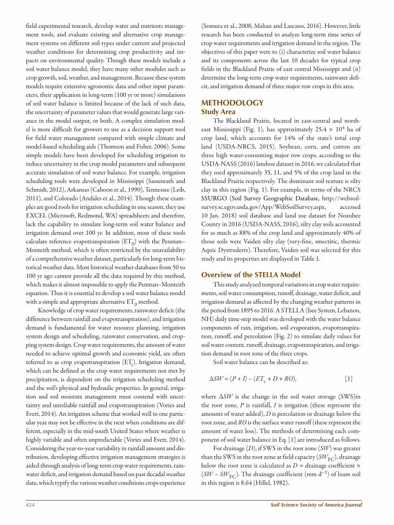
The Blackland Prairie, located in east-central and north-east Mississippi (Fig. 1), has approximately 25.4 × 10⁴ ha of crop land, which accounts for 14% of the state’s total crop land (USDA-NRCS, 2015). Soybean, corn, and cotton are three high water-consuming major row crops, according to the USDA-NASS (2016) landuse dataset in 2016, we calculated that they used approximately 35, 11, and 5% of the crop land in the Blackland Prairie respectively. The dominant soil texture is silty clay in this region (Fig. 1). For example, in terms of the NRCS SSURGO (Soil Survey Geographic Database, http://websoil-survey.sc.egov.usda.gov/App/WebSoilSurvey.aspx, accessed 10 Jan. 2018) soil database and land use dataset for Noxubee County in 2016 (USDA-NASS, 2016), silty clay soils accounted for as much as 88% of the crop land and approximately 40% of those soils were Vaiden silty clay (very-fine, smectitic, thermic Aquic Dystruderts). Therefore, Vaiden soil was selected for this study and its properties are displayed in Table 1.
Overview of the STELLA Model This study analyzed temporal variations in crop water require-
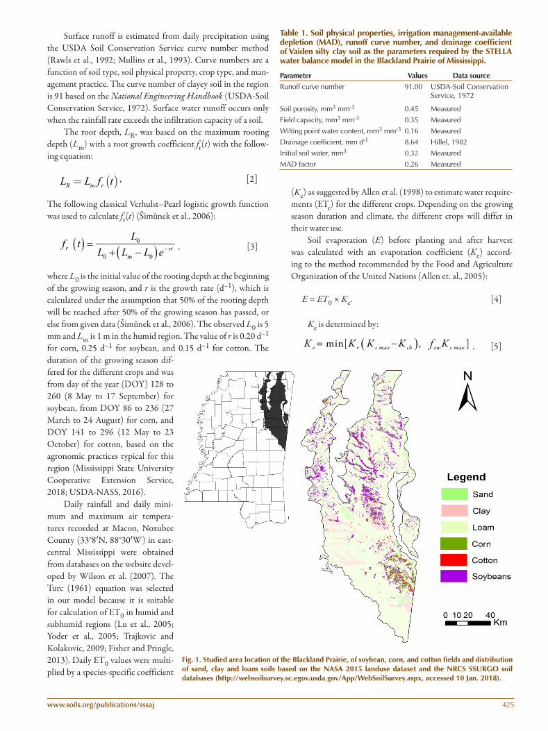
ments, soil water consumption, runoff, drainage, water deficit, and irrigation demand as affected by the changing weather patterns in the period from 1895 to 2016. A STELLA (Isee System, Lebanon, NH) daily time-step model was developed with the water balance components of rain, irrigation, soil evaporation, evapotranspira-tion, runoff, and percolation (Fig. 2) to simulate daily values for soil water content, runoff, drainage, evapotranspiration, and irriga-tion demand in root zone of the three crops.
Soil water balance can be described as:
∆SW = (P + I) – (ETc + D + RO), [1]
where ∆SW is the change in the soil water storage (SWS)in the root zone, P is rainfall, I is irrigation (these represent the amounts of water added), D is percolation or drainage below the root zone, and RO is the surface water runoff (these represent the amount of water loss). The methods of determining each com-ponent of soil water balance in Eq. [1] are introduced as follows.
For drainage (D), if SWS in the root zone (SW) was greater than the SWS in the root zone at field capacity (SWFC), drainage below the root zone is calculated as D = drainage coefficient × (SW – SWFC). The drainage coefficient (mm d–1) of loam soil in this region is 8.64 (Hillel, 1982).
www.soils.org/publications/sssaj 425
Surface runoff is estimated from daily precipitation using the USDA Soil Conservation Service curve number method (Rawls et al., 1992; Mullins et al., 1993). Curve numbers are a function of soil type, soil physical property, crop type, and man-agement practice. The curve number of clayey soil in the region is 91 based on the National Engineering Handbook (USDA-Soil Conservation Service, 1972). Surface water runoff occurs only when the rainfall rate exceeds the infiltration capacity of a soil.
The root depth, LR, was based on the maximum rooting depth (Lm) with a root growth coefficient fr(t) with the follow-ing equation:
( )R m rL L f t= , [2]
The following classical Verhulst–Pearl logistic growth function was used to calculate fr(t) (Šimůnek et al., 2006):
( ) ( )0
0 0
r rtm
Lf tL L L e-=+ - , [3]
where L0 is the initial value of the rooting depth at the beginning of the growing season, and r is the growth rate (d–1), which is calculated under the assumption that 50% of the rooting depth will be reached after 50% of the growing season has passed, or else from given data (Šimůnek et al., 2006). The observed L0 is 5 mm and Lm is 1 m in the humid region. The value of r is 0.20 d–1 for corn, 0.25 d–1 for soybean, and 0.15 d–1 for cotton. The duration of the growing season dif-fered for the different crops and was from day of the year (DOY) 128 to 260 (8 May to 17 September) for soybean, from DOY 86 to 236 (27 March to 24 August) for corn, and DOY 141 to 296 (12 May to 23 October) for cotton, based on the agronomic practices typical for this region (Mississippi State University Cooperative Extension Service, 2018; USDA-NASS, 2016).
Daily rainfall and daily mini-mum and maximum air tempera-tures recorded at Macon, Noxubee County (33°8¢N, 88°30¢W) in east-central Mississippi were obtained from databases on the website devel-oped by Wilson et al. (2007). The Turc (1961) equation was selected in our model because it is suitable for calculation of ET0 in humid and subhumid regions (Lu et al., 2005; Yoder et al., 2005; Trajkovic and Kolakovic, 2009; Fisher and Pringle, 2013). Daily ET0 values were multi-plied by a species-specific coefficient
(Kc) as suggested by Allen et al. (1998) to estimate water require-ments (ETc) for the different crops. Depending on the growing season duration and climate, the different crops will differ in their water use.
Soil evaporation (E) before planting and after harvest was calculated with an evaporation coefficient (Ke) accord-ing to the method recommended by the Food and Agriculture Organization of the United Nations (Allen et. al., 2005):
E = ET0 × Ke. [4]
Ke is determined by:
( ) min[ , ] e r c max cb ew c maxK K K K f K= - , [5]
Table 1. Soil physical properties, irrigation management-available depletion (MAD), runoff curve number, and drainage coefficient of Vaiden silty clay soil as the parameters required by the STELLA water balance model in the Blackland Prairie of Mississippi.
Parameter Values Data source
Runoff curve number 91.00 USDA-Soil Conservation Service, 1972
Soil porosity, mm3 mm-3 0.45 Measured
Field capacity, mm3 mm-3 0.35 Measured
Wilting point water content, mm3 mm-3 0.16 Measured
Drainage coefficient, mm d-1 8.64 Hillel, 1982
Initial soil water, mm3 0.32 Measured
MAD factor 0.26 Measured
Fig. 1. Studied area location of the Blackland Prairie, of soybean, corn, and cotton fields and distribution of sand, clay and loam soils based on the NASA 2015 landuse dataset and the NRCS SSURGO soil databases (http://websoilsurvey.sc.egov.usda.gov/App/WebSoilSurvey.aspx, accessed 10 Jan. 2018).
426 Soil Science Society of America Journal
where Kcb is basal crop coefficient, Kc max is the maximum value of Kc following rain or irrigation, Kr is a dimensionless evapora-tion reduction coefficient dependent on the cumulative depth of water depleted (evaporated) from the topsoil, and few is the frac-tion of the soil that is both exposed and wetted, which is 1 for bare soil. Allen et al. (1998) suggested a Kc max value of 1.2 for the humid mid-south United States, where irrigation or precipi-tation events are more frequent. A Kcb value of zero was used for bare soils without crops.
The potential available water content or storage (AWC) in the rooting zone is calculated as:
AWC = SWFC – SWWP , [6]
where SWFC and SWWP are soil water content at soil field capacity and the crop permanent wilting point multiplied by rooting depth.
Management allowable depletion is a certain percentage of AWC. It is often used as an irrigation trigger point. Management allowable depletion is commonly set as 50% of AWC in root zone (Suttles et al., 1999; Ozdogan et al., 2010; Andales et al., 2014); therefore, we adopted half the AWC in the root zone as our trigger point of any irrigation for determining irrigation timing. Sufficient irrigation water was required to replenish soil moisture to field capacity in the root zone. Irrigation demand was calculated as the difference in SWS in a 1-m profile at field capacity and right before irrigation as triggered and required. The frequency of irrigation demand for each day during the growing season was calculated as the total number of irrigations on a given day divided by 122, the number of times that DOY occurred in 122 yr as simulated with the STELLA model. For example, the total number of irrigation events on DOY 200 was
12 for corn and thus the frequency of corn irrigation demand on that day was 12 out of 122, which is 10%. A similar approach was used by Pote and Wax (1986) and Tang et al. (2017) to analyze the irrigation demand and frequency of row crops in the Mississippi Delta region. A rainwater deficit or surplus was calculated by the difference between rainfall and ETc in a given period of time, whereas total effective rainwater deficit or surplus was the result of rainfall minus runoff, percolation, and ETc.
Classifying Wet, Normal, and Dry YearsIt is common to classify historical long-term time-series
meteorological data according to ‘wet’, ‘normal’, and ‘dry’ years for studies on drought and water management (Lloyd-Hughes and Saunders, 2002). Previous studies (Wang et al., 2009; Liu et al., 2013; Zhang et al., 2013) applied the frequency analysis method to characterize a given number of years to wet, normal, and dry years based on the amount of rainfall over a certain pe-riod of time. In our study, this frequency analysis method was used to classify the 122 yr from 1895 to 2016 according to wet, normal, and dry years to better evaluate rainfall deficit and hence the annual irrigation demand. First, values for annual rainfall and growing season rainfall in each of the 122 yr (n = 122) were ranked from largest to lowest and were labeled according to rank (m). Second, the probability (P) was calculated for each ranked year (m) as: P = m (n + 1)–1 × 100%. Third, each calendar year was categorized as wet if P ≤ 25%, as normal if 25% < P < 75%, and as dry if P ≥ 75%. As a result, there were 30, 31, or 32 wet or dry years and 60 or 61 normal years.
Fig. 2. A schematic diagram showing the field water balance components used for developing the Structural Thinking and Experiential Learning Laboratory with Animation (STELLA) model.
www.soils.org/publications/sssaj 427
Evaluation of the STELLA Model The soybean, corn, and cotton field experiments were con-
ducted on a private farm and at the Mississippi State University Black Belt Branch Station in Noxubee County, MS, in 2014, 2015, and 2016. These fields contain Brooksville (fine, smec-titic, thermic Aquic Hapluderts) and Vaiden silty clay soils. Soil water content at depths of 15, 30, 60, and 90 cm was measured periodically each year by either the gravimetric method or Time Domain Reflectometer soil moisture sensors (Acclima Inc., Meridian, ID). Microflume runoff collectors (Franklin et al., 2001) were installed at the tail end of the fields. The measured soil water content and runoff from 2014 to 2016 were used to validate the STELLA soil water balance model. We evaluated the simulation results with the relative root mean squared deviation normalized the difference between the simulated and observed values to the mean of the observed values (0–1) and the mean ab-solute error (MAE) between the measured and simulated values (Legates, 1999; Ma et al., 2012):
( )2
1
avg
1 Ni ii
P ONRRMSD
O=
-=
∑ ; [7]
1
Ni ii
P OMAE
N=
-= ∑ , [8]
where, Pi is the ith simulated value, Oi is the ith observed value, Oavg is the average of the observed values, and n is the number of data pairs.
RESULTSRainfall and Frequency
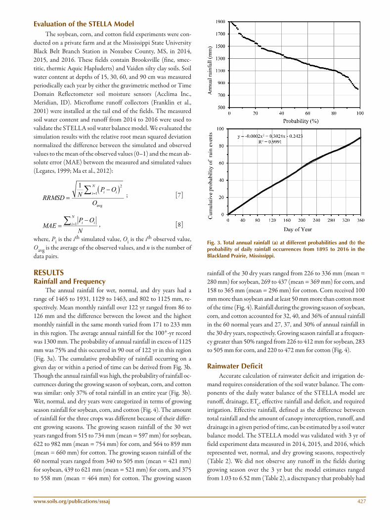
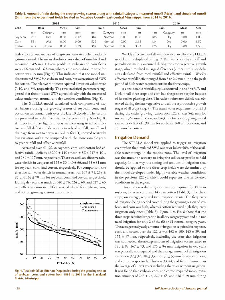
The annual rainfall for wet, normal, and dry years had a range of 1465 to 1931, 1129 to 1463, and 802 to 1125 mm, re-spectively. Mean monthly rainfall over 122 yr ranged from 86 to 126 mm and the difference between the lowest and the highest monthly rainfall in the same month varied from 171 to 233 mm in this region. The average annual rainfall for the 100+-yr record was 1300 mm. The probability of annual rainfall in excess of 1125 mm was 75% and this occurred in 90 out of 122 yr in this region (Fig. 3a). The cumulative probability of rainfall occurring on a given day or within a period of time can be derived from Fig. 3b. Though the annual rainfall was high, the probability of rainfall oc-currences during the growing season of soybean, corn, and cotton was similar: only 37% of total rainfall in an entire year (Fig. 3b). Wet, normal, and dry years were categorized in terms of growing season rainfall for soybean, corn, and cotton (Fig. 4). The amount of rainfall for the three crops was different because of their differ-ent growing seasons. The growing season rainfall of the 30 wet years ranged from 515 to 734 mm (mean = 597 mm) for soybean, 622 to 982 mm (mean = 754 mm) for corn, and 564 to 859 mm (mean = 660 mm) for cotton. The growing season rainfall of the 60 normal years ranged from 340 to 505 mm (mean = 421 mm) for soybean, 439 to 621 mm (mean = 521 mm) for corn, and 375 to 558 mm (mean = 464 mm) for cotton. The growing season
rainfall of the 30 dry years ranged from 226 to 336 mm (mean = 280 mm) for soybean, 269 to 437 (mean = 369 mm) for corn, and 158 to 365 mm (mean = 296 mm) for cotton. Corn received 100 mm more than soybean and at least 50 mm more than cotton most of the time (Fig. 4). Rainfall during the growing season of soybean, corn, and cotton accounted for 32, 40, and 36% of annual rainfall in the 60 normal years and 27, 37, and 30% of annual rainfall in the 30 dry years, respectively. Growing season rainfall at a frequen-cy greater than 50% ranged from 226 to 412 mm for soybean, 283 to 505 mm for corn, and 220 to 472 mm for cotton (Fig. 4).
Rainwater DeficitAccurate calculation of rainwater deficit and irrigation de-
mand requires consideration of the soil water balance. The com-ponents of the daily water balance of the STELLA model are runoff, drainage, ETc, effective rainfall and deficit, and required irrigation. Effective rainfall, defined as the difference between total rainfall and the amount of canopy interception, runoff, and drainage in a given period of time, can be estimated by a soil water balance model. The STELLA model was validated with 3 yr of field experiment data measured in 2014, 2015, and 2016, which represented wet, normal, and dry growing seasons, respectively (Table 2). We did not observe any runoff in the fields during growing season over the 3 yr but the model estimates ranged from 1.03 to 6.52 mm (Table 2), a discrepancy that probably had
Fig. 3. Total annual rainfall (a) at different probabilities and (b) the probability of daily rainfall occurrences from 1895 to 2016 in the Blackland Prairie, Mississippi.
428 Soil Science Society of America Journal
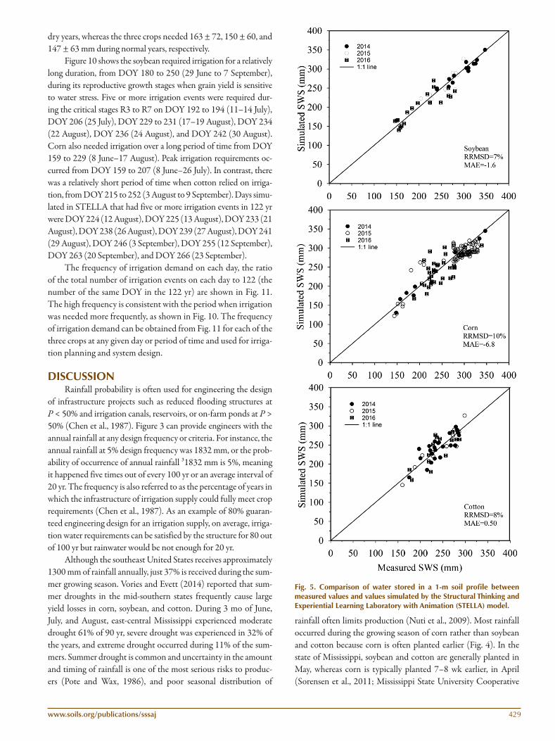
little effect on our analysis of long-term rainwater deficit and irri-gation demand. The mean absolute error values of simulated and measured SWS in a 100-cm profile in soybean and corn fields were -1.6 mm and −6.8 mm, whereas the mean absolute error for cotton was 0.5 mm (Fig. 5). This indicated that the model un-derestimated SWS for soybean and corn, but overestimated SWS for cotton. The relative root mean squared deviation values were 7, 10, and 8%, respectively. The two statistical parameters sug-gested that the simulated SWS agreed closely with the measured values under wet, normal, and dry weather conditions (Fig. 5).
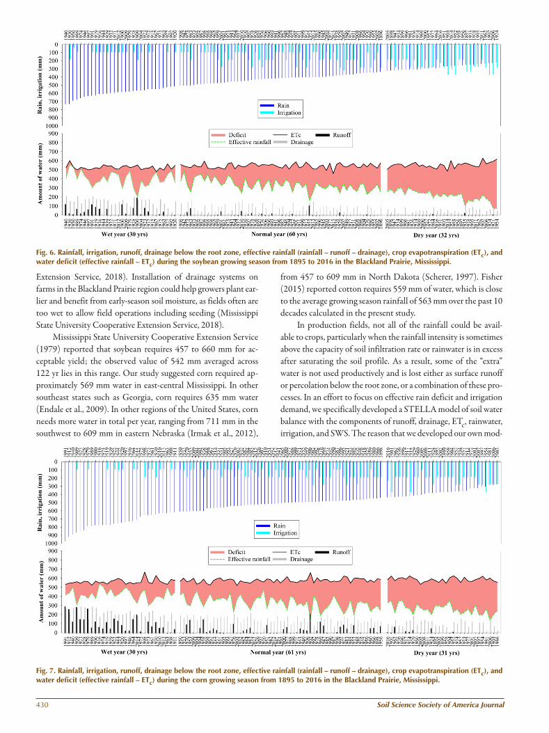
The STELLA model calculated each component of wa-ter balance during the growing season of soybean, corn, and cotton on an annual basis over the last 10 decades. The results are presented in order from wet to dry years in Fig. 6 to Fig. 8. As expected, these figures display an increasing trend of effec-tive rainfall deficit and decreasing trends of rainfall, runoff, and drainage from wet to dry years. Values for ETc showed relatively low variation with time compared with the more variable year-to-year rainfall and effective rainfall.
Averaged over all 122 yr, soybean, corn, and cotton had ef-fective rainfall deficits of 200 ± 110 (mean ± SD), 217 ± 101, and 184 ± 117 mm, respectively. There was still an effective rain-water deficit in wet years of 122 ± 80, 140 ± 66, and 95 ± 81 mm for soybean, corn, and cotton, respectively. For comparison, the effective rainwater deficit in normal years was 209 ± 71, 238 ± 85, and 163 ± 70 mm for soybean, corn, and cotton, respectively. During dry years, as much as 340 ± 76, 324 ± 60, and 327 ± 65 mm effective rainwater deficit was calculated for soybean, corn, and cotton growing seasons ,respectively.
Weekly effective rainfall was also calculated by the STELLA model and is displayed in Fig. 9. Rainwater loss by runoff and percolation mainly occurred during the crop vegetative growth stage, which resulted in large differences (either surplus or defi-cit) calculated from total rainfall and effective rainfall. Weekly effective rainfall deficit ranged from 8 to 26 mm during the peak period of high water requirements in the three crops.
A considerable rainfall surplus occurred in the first 5, 7, and 8 wk for all three crops and corn had the greatest surplus because of its earlier planting date. Thereafter, rainwater deficit was ob-served during the late vegetative and all the reproductive growth stages of all crops (Fig. 9). The mean water requirement (or ETc) during the entire growing season over 122 yr was 542 mm for soybean, 569 mm for corn, and 563 mm for cotton, giving a total rainwater deficit of 190 mm for soybean, 168 mm for corn, and 150 mm for cotton.
Irrigation DemandThe STELLA model was applied to trigger an irrigation
event when the simulated SWS was at or below 50% of the avail-able water storage in the rooting zone. The level of irrigation was the amount necessary to bring the soil water profile to field capacity. In that way, the timing and amount of irrigation that should be applied to the three crop fields were determined by the model developed under highly variable weather conditions in the previous 122 yr, which could represent diverse weather conditions in the region.
This study revealed irrigation was not required for 12 yr in soybean, 17 yr in corn, and 14 yr in cotton (Table 3). The three crops, on average, required two irrigation events. The frequency of irrigation being needed twice during the growing season of soy-bean and corn was high, whereas cotton required high-frequency irrigation only once (Table 3). Figure 6 to Fig. 8 show that the three crops required irrigation in all dry category years and did not need irrigation for only 2 of the 60 or 61 normal category years. The average total yearly amount of irrigation required for soybean, corn, and cotton over the 122 yr was 162 ± 100, 143 ± 89, and 155 ± 97 mm, respectively. Excluding the years that irrigation was not needed, the average amount of irrigation was increased to 180 ± 89, 167 ± 73, and 175 ± 84 mm. Irrigation in wet years was generally not required and the average amount of all irrigation events was 99 ± 32, 104 ± 33, and 130 ± 55 mm for soybean, corn, and cotton, respectively. This was 33, 44, and 62 mm more than the average of all wet years including the years without irrigation. It was found that soybean, corn, and cotton required mean irriga-tion amounts of 266 ± 72, 229 ± 68, and 258 ± 79 mm during
Table 2. Amount of rain during the crop growing season along with rainfall category, measured runoff (Meas), and simulated runoff (Sim) from the experiment fields located in Noxubee County, east-central Mississippi, from 2014 to 2016.
Crop
2014 2015 2016
Rain Meas Sim Rain Meas Sim Rain Meas Sim
mm Category mm mm mm Category mm mm mm Category mm mm
Cotton 435 Normal 0.00 3.79 397 Normal 0.00 3.93 275 Dry 0.00 2.53
Fig. 4. Total rainfall at different frequencies during the growing season of soybean, corn, and cotton from 1895 to 2016 in the Blackland Prairie, Mississippi.
www.soils.org/publications/sssaj 429
dry years, whereas the three crops needed 163 ± 72, 150 ± 60, and 147 ± 63 mm during normal years, respectively.
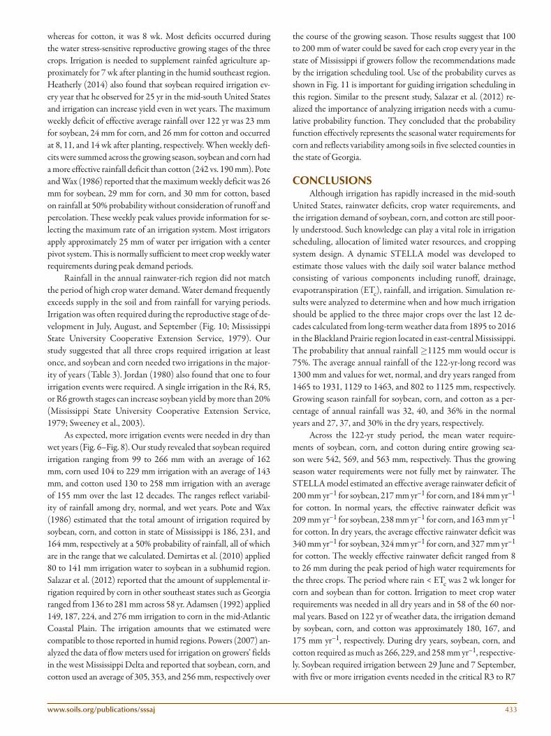
Figure 10 shows the soybean required irrigation for a relatively long duration, from DOY 180 to 250 (29 June to 7 September), during its reproductive growth stages when grain yield is sensitive to water stress. Five or more irrigation events were required dur-ing the critical stages R3 to R7 on DOY 192 to 194 (11–14 July), DOY 206 (25 July), DOY 229 to 231 (17–19 August), DOY 234 (22 August), DOY 236 (24 August), and DOY 242 (30 August). Corn also needed irrigation over a long period of time from DOY 159 to 229 (8 June–17 August). Peak irrigation requirements oc-curred from DOY 159 to 207 (8 June–26 July). In contrast, there was a relatively short period of time when cotton relied on irriga-tion, from DOY 215 to 252 (3 August to 9 September). Days simu-lated in STELLA that had five or more irrigation events in 122 yr were DOY 224 (12 August), DOY 225 (13 August), DOY 233 (21 August), DOY 238 (26 August), DOY 239 (27 August), DOY 241 (29 August), DOY 246 (3 September), DOY 255 (12 September), DOY 263 (20 September), and DOY 266 (23 September).
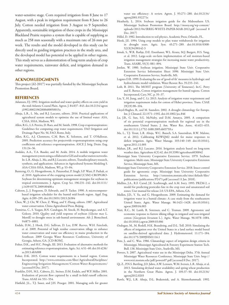
The frequency of irrigation demand on each day, the ratio of the total number of irrigation events on each day to 122 (the number of the same DOY in the 122 yr) are shown in Fig. 11. The high frequency is consistent with the period when irrigation was needed more frequently, as shown in Fig. 10. The frequency of irrigation demand can be obtained from Fig. 11 for each of the three crops at any given day or period of time and used for irriga-tion planning and system design.
DISCUSSIONRainfall probability is often used for engineering the design
of infrastructure projects such as reduced flooding structures at P < 50% and irrigation canals, reservoirs, or on-farm ponds at P > 50% (Chen et al., 1987). Figure 3 can provide engineers with the annual rainfall at any design frequency or criteria. For instance, the annual rainfall at 5% design frequency was 1832 mm, or the prob-ability of occurrence of annual rainfall ³1832 mm is 5%, meaning it happened five times out of every 100 yr or an average interval of 20 yr. The frequency is also referred to as the percentage of years in which the infrastructure of irrigation supply could fully meet crop requirements (Chen et al., 1987). As an example of 80% guaran-teed engineering design for an irrigation supply, on average, irriga-tion water requirements can be satisfied by the structure for 80 out of 100 yr but rainwater would be not enough for 20 yr.
Although the southeast United States receives approximately 1300 mm of rainfall annually, just 37% is received during the sum-mer growing season. Vories and Evett (2014) reported that sum-mer droughts in the mid-southern states frequently cause large yield losses in corn, soybean, and cotton. During 3 mo of June, July, and August, east-central Mississippi experienced moderate drought 61% of 90 yr, severe drought was experienced in 32% of the years, and extreme drought occurred during 11% of the sum-mers. Summer drought is common and uncertainty in the amount and timing of rainfall is one of the most serious risks to produc-ers (Pote and Wax, 1986), and poor seasonal distribution of
rainfall often limits production (Nuti et al., 2009). Most rainfall occurred during the growing season of corn rather than soybean and cotton because corn is often planted earlier (Fig. 4). In the state of Mississippi, soybean and cotton are generally planted in May, whereas corn is typically planted 7–8 wk earlier, in April (Sorensen et al., 2011; Mississippi State University Cooperative
Fig. 5. Comparison of water stored in a 1-m soil profile between measured values and values simulated by the Structural Thinking and Experiential Learning Laboratory with Animation (STELLA) model.
430 Soil Science Society of America Journal
Extension Service, 2018). Installation of drainage systems on farms in the Blackland Prairie region could help growers plant ear-lier and benefit from early-season soil moisture, as fields often are too wet to allow field operations including seeding (Mississippi State University Cooperative Extension Service, 2018).
Mississippi State University Cooperative Extension Service (1979) reported that soybean requires 457 to 660 mm for ac-ceptable yield; the observed value of 542 mm averaged across 122 yr lies in this range. Our study suggested corn required ap-proximately 569 mm water in east-central Mississippi. In other southeast states such as Georgia, corn requires 635 mm water (Endale et al., 2009). In other regions of the United States, corn needs more water in total per year, ranging from 711 mm in the southwest to 609 mm in eastern Nebraska (Irmak et al., 2012),
from 457 to 609 mm in North Dakota (Scherer, 1997). Fisher (2015) reported cotton requires 559 mm of water, which is close to the average growing season rainfall of 563 mm over the past 10 decades calculated in the present study.
In production fields, not all of the rainfall could be avail-able to crops, particularly when the rainfall intensity is sometimes above the capacity of soil infiltration rate or rainwater is in excess after saturating the soil profile. As a result, some of the “extra” water is not used productively and is lost either as surface runoff or percolation below the root zone, or a combination of these pro-cesses. In an effort to focus on effective rain deficit and irrigation demand, we specifically developed a STELLA model of soil water balance with the components of runoff, drainage, ETc, rainwater, irrigation, and SWS. The reason that we developed our own mod-
Fig. 6. Rainfall, irrigation, runoff, drainage below the root zone, effective rainfall (rainfall – runoff – drainage), crop evapotranspiration (ETc), and water deficit (effective rainfall – ETc) during the soybean growing season from 1895 to 2016 in the Blackland Prairie, Mississippi.
Fig. 7. Rainfall, irrigation, runoff, drainage below the root zone, effective rainfall (rainfall – runoff – drainage), crop evapotranspiration (ETc), and water deficit (effective rainfall – ETc) during the corn growing season from 1895 to 2016 in the Blackland Prairie, Mississippi.
www.soils.org/publications/sssaj 431
el was so we could use a century-long historical weather dataset and specify an ET0 method for our unique objectives. The main difference between our model and some existing models for esti-mating irrigation amounts is that the irrigation water demand was estimated from long-term historical weather records and a speci-fied Turc method for ET0 calculation. The objective of this study was to estimate the general and average rainwater deficit in this area so that we can obtain “conservative” crop irrigation demand values that would fully satisfy crop water requirements. Different drought tolerant cultivars or hybrids were not considered in the present study, so further research is needed to characterize changes in irrigation demand with improved crop cultivars for this region during the past 122 yr. Historical weather data were used as model input to capture the variability of weather conditions and hence to determine irrigation demand as affected by all different types of wet, normal, and dry weather conditions. This approach has been widely used by other researchers. It is common in the model-ing research community to use long-term historical weather data for considering various weather conditions to investigate a certain given hybrid. For example, Saseendran et al. (2008) applied the CERES-maize (i.e. for corn) model with a long-term weather record from 1912 to 2005 to determine the optimum alloca-tion of limited irrigation and the optimum soil water depletion level for initiating irrigation for the corn hybrid ‘Pioneer Brand 3732’ in Colorado. Qi et al. (2013) used a 50-yr weather dataset (1961–2010) and Root Zone Water Quality Model (Ahuja et al., 2016) to assess the long-term impacts of management prac-tices on a spring wheat hybrid, ‘DS3585’ in Montana. Banterng et al. (2010) used 32-yr historical weather data (1972–2003) and the CSM-CROPGRO-Soybean model to predict the optimum management practices for the production of one soybean cultivar in tropical environments. Saseendran et al. (2016) used weather
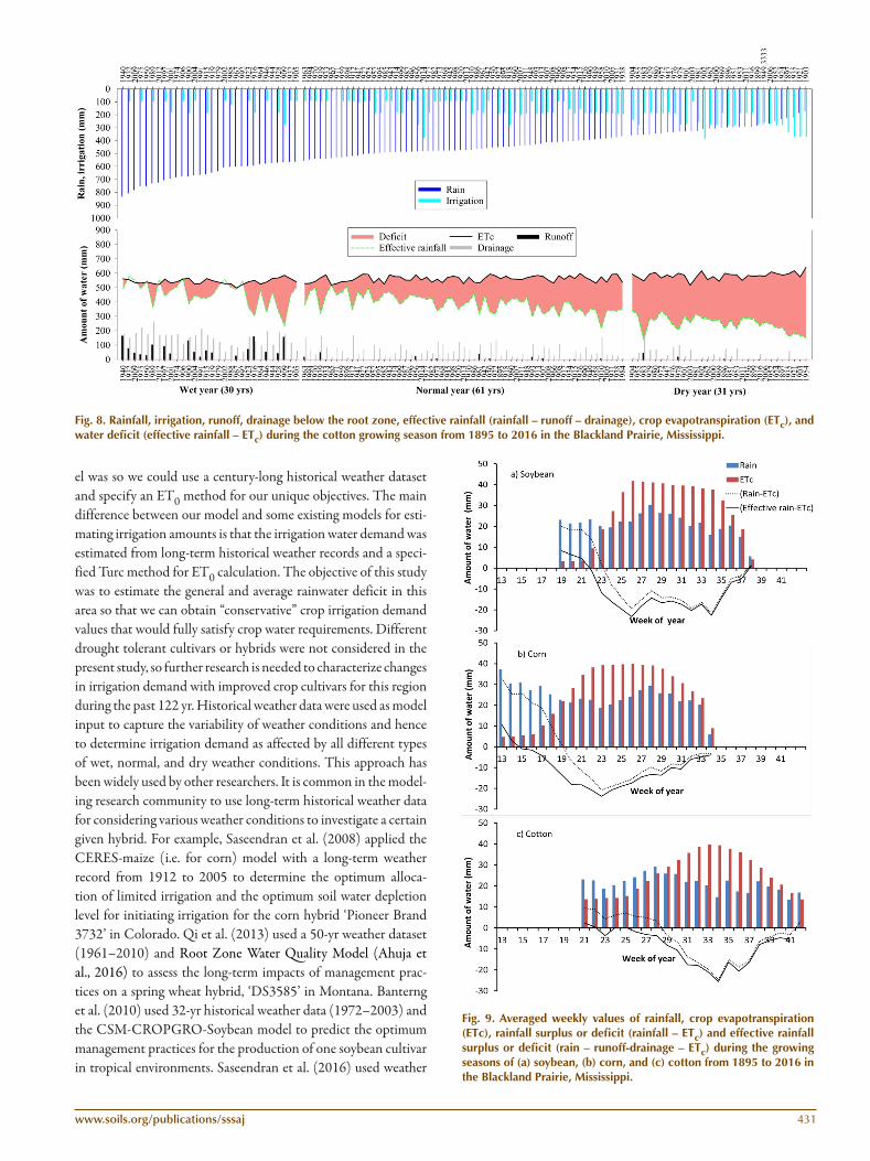
Fig. 8. Rainfall, irrigation, runoff, drainage below the root zone, effective rainfall (rainfall – runoff – drainage), crop evapotranspiration (ETc), and water deficit (effective rainfall – ETc) during the cotton growing season from 1895 to 2016 in the Blackland Prairie, Mississippi.
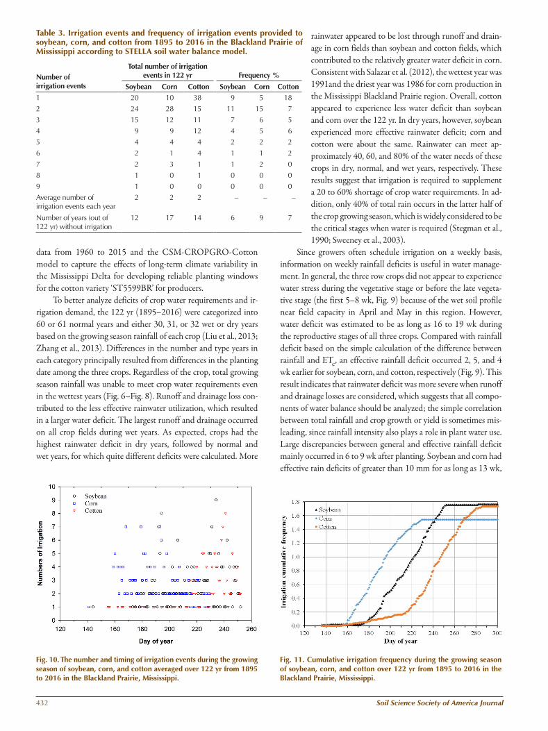
Fig. 9. Averaged weekly values of rainfall, crop evapotranspiration (ETc), rainfall surplus or deficit (rainfall – ETc) and effective rainfall surplus or deficit (rain – runoff-drainage – ETc) during the growing seasons of (a) soybean, (b) corn, and (c) cotton from 1895 to 2016 in the Blackland Prairie, Mississippi.
432 Soil Science Society of America Journal
data from 1960 to 2015 and the CSM-CROPGRO-Cotton model to capture the effects of long-term climate variability in the Mississippi Delta for developing reliable planting windows for the cotton variety ‘ST5599BR’ for producers.
To better analyze deficits of crop water requirements and ir-rigation demand, the 122 yr (1895–2016) were categorized into 60 or 61 normal years and either 30, 31, or 32 wet or dry years based on the growing season rainfall of each crop (Liu et al., 2013; Zhang et al., 2013). Differences in the number and type years in each category principally resulted from differences in the planting date among the three crops. Regardless of the crop, total growing season rainfall was unable to meet crop water requirements even in the wettest years (Fig. 6–Fig. 8). Runoff and drainage loss con-tributed to the less effective rainwater utilization, which resulted in a larger water deficit. The largest runoff and drainage occurred on all crop fields during wet years. As expected, crops had the highest rainwater deficit in dry years, followed by normal and wet years, for which quite different deficits were calculated. More
rainwater appeared to be lost through runoff and drain-age in corn fields than soybean and cotton fields, which contributed to the relatively greater water deficit in corn. Consistent with Salazar et al. (2012), the wettest year was 1991and the driest year was 1986 for corn production in the Mississippi Blackland Prairie region. Overall, cotton appeared to experience less water deficit than soybean and corn over the 122 yr. In dry years, however, soybean experienced more effective rainwater deficit; corn and cotton were about the same. Rainwater can meet ap-proximately 40, 60, and 80% of the water needs of these crops in dry, normal, and wet years, respectively. These results suggest that irrigation is required to supplement a 20 to 60% shortage of crop water requirements. In ad-dition, only 40% of total rain occurs in the latter half of the crop growing season, which is widely considered to be the critical stages when water is required (Stegman et al., 1990; Sweeney et al., 2003).
Since growers often schedule irrigation on a weekly basis, information on weekly rainfall deficits is useful in water manage-ment. In general, the three row crops did not appear to experience water stress during the vegetative stage or before the late vegeta-tive stage (the first 5–8 wk, Fig. 9) because of the wet soil profile near field capacity in April and May in this region. However, water deficit was estimated to be as long as 16 to 19 wk during the reproductive stages of all three crops. Compared with rainfall deficit based on the simple calculation of the difference between rainfall and ETc, an effective rainfall deficit occurred 2, 5, and 4 wk earlier for soybean, corn, and cotton, respectively (Fig. 9). This result indicates that rainwater deficit was more severe when runoff and drainage losses are considered, which suggests that all compo-nents of water balance should be analyzed; the simple correlation between total rainfall and crop growth or yield is sometimes mis-leading, since rainfall intensity also plays a role in plant water use. Large discrepancies between general and effective rainfall deficit mainly occurred in 6 to 9 wk after planting. Soybean and corn had effective rain deficits of greater than 10 mm for as long as 13 wk,
Table 3. Irrigation events and frequency of irrigation events provided to soybean, corn, and cotton from 1895 to 2016 in the Blackland Prairie of Mississippi according to STELLA soil water balance model.
Number of irrigation events
Total number of irrigation events in 122 yr
Frequency %
Soybean Corn Cotton Soybean Corn Cotton
1 20 10 38 9 5 18
2 24 28 15 11 15 7
3 15 12 11 7 6 5
4 9 9 12 4 5 6
5 4 4 4 2 2 2
6 2 1 4 1 1 2
7 2 3 1 1 2 0
8 1 0 1 0 0 0
9 1 0 0 0 0 0
Average number of irrigation events each year
2 2 2 – – –
Number of years (out of 122 yr) without irrigation
12 17 14 6 9 7
Fig. 10. The number and timing of irrigation events during the growing season of soybean, corn, and cotton averaged over 122 yr from 1895 to 2016 in the Blackland Prairie, Mississippi.
Fig. 11. Cumulative irrigation frequency during the growing season of soybean, corn, and cotton over 122 yr from 1895 to 2016 in the Blackland Prairie, Mississippi.
www.soils.org/publications/sssaj 433
whereas for cotton, it was 8 wk. Most deficits occurred during the water stress-sensitive reproductive growing stages of the three crops. Irrigation is needed to supplement rainfed agriculture ap-proximately for 7 wk after planting in the humid southeast region. Heatherly (2014) also found that soybean required irrigation ev-ery year that he observed for 25 yr in the mid-south United States and irrigation can increase yield even in wet years. The maximum weekly deficit of effective average rainfall over 122 yr was 23 mm for soybean, 24 mm for corn, and 26 mm for cotton and occurred at 8, 11, and 14 wk after planting, respectively. When weekly defi-cits were summed across the growing season, soybean and corn had a more effective rainfall deficit than cotton (242 vs. 190 mm). Pote and Wax (1986) reported that the maximum weekly deficit was 26 mm for soybean, 29 mm for corn, and 30 mm for cotton, based on rainfall at 50% probability without consideration of runoff and percolation. These weekly peak values provide information for se-lecting the maximum rate of an irrigation system. Most irrigators apply approximately 25 mm of water per irrigation with a center pivot system. This is normally sufficient to meet crop weekly water requirements during peak demand periods.
Rainfall in the annual rainwater-rich region did not match the period of high crop water demand. Water demand frequently exceeds supply in the soil and from rainfall for varying periods. Irrigation was often required during the reproductive stage of de-velopment in July, August, and September (Fig. 10; Mississippi State University Cooperative Extension Service, 1979). Our study suggested that all three crops required irrigation at least once, and soybean and corn needed two irrigations in the major-ity of years (Table 3). Jordan (1980) also found that one to four irrigation events were required. A single irrigation in the R4, R5, or R6 growth stages can increase soybean yield by more than 20% (Mississippi State University Cooperative Extension Service, 1979; Sweeney et al., 2003).
As expected, more irrigation events were needed in dry than wet years (Fig. 6–Fig. 8). Our study revealed that soybean required irrigation ranging from 99 to 266 mm with an average of 162 mm, corn used 104 to 229 mm irrigation with an average of 143 mm, and cotton used 130 to 258 mm irrigation with an average of 155 mm over the last 12 decades. The ranges reflect variabil-ity of rainfall among dry, normal, and wet years. Pote and Wax (1986) estimated that the total amount of irrigation required by soybean, corn, and cotton in state of Mississippi is 186, 231, and 164 mm, respectively at a 50% probability of rainfall, all of which are in the range that we calculated. Demirtas et al. (2010) applied 80 to 141 mm irrigation water to soybean in a subhumid region. Salazar et al. (2012) reported that the amount of supplemental ir-rigation required by corn in other southeast states such as Georgia ranged from 136 to 281 mm across 58 yr. Adamsen (1992) applied 149, 187, 224, and 276 mm irrigation to corn in the mid-Atlantic Coastal Plain. The irrigation amounts that we estimated were compatible to those reported in humid regions. Powers (2007) an-alyzed the data of flow meters used for irrigation on growers’ fields in the west Mississippi Delta and reported that soybean, corn, and cotton used an average of 305, 353, and 256 mm, respectively over
the course of the growing season. Those results suggest that 100 to 200 mm of water could be saved for each crop every year in the state of Mississippi if growers follow the recommendations made by the irrigation scheduling tool. Use of the probability curves as shown in Fig. 11 is important for guiding irrigation scheduling in this region. Similar to the present study, Salazar et al. (2012) re-alized the importance of analyzing irrigation needs with a cumu-lative probability function. They concluded that the probability function effectively represents the seasonal water requirements for corn and reflects variability among soils in five selected counties in the state of Georgia.
CONCLUSIONSAlthough irrigation has rapidly increased in the mid-south
United States, rainwater deficits, crop water requirements, and the irrigation demand of soybean, corn, and cotton are still poor-ly understood. Such knowledge can play a vital role in irrigation scheduling, allocation of limited water resources, and cropping system design. A dynamic STELLA model was developed to estimate those values with the daily soil water balance method consisting of various components including runoff, drainage, evapotranspiration (ETc), rainfall, and irrigation. Simulation re-sults were analyzed to determine when and how much irrigation should be applied to the three major crops over the last 12 de-cades calculated from long-term weather data from 1895 to 2016 in the Blackland Prairie region located in east-central Mississippi. The probability that annual rainfall ³1125 mm would occur is 75%. The average annual rainfall of the 122-yr-long record was 1300 mm and values for wet, normal, and dry years ranged from 1465 to 1931, 1129 to 1463, and 802 to 1125 mm, respectively. Growing season rainfall for soybean, corn, and cotton as a per-centage of annual rainfall was 32, 40, and 36% in the normal years and 27, 37, and 30% in the dry years, respectively.
Across the 122-yr study period, the mean water require-ments of soybean, corn, and cotton during entire growing sea-son were 542, 569, and 563 mm, respectively. Thus the growing season water requirements were not fully met by rainwater. The STELLA model estimated an effective average rainwater deficit of 200 mm yr–1 for soybean, 217 mm yr–1 for corn, and 184 mm yr–1 for cotton. In normal years, the effective rainwater deficit was 209 mm yr–1 for soybean, 238 mm yr–1 for corn, and 163 mm yr–1 for cotton. In dry years, the average effective rainwater deficit was 340 mm yr–1 for soybean, 324 mm yr–1 for corn, and 327 mm yr–1 for cotton. The weekly effective rainwater deficit ranged from 8 to 26 mm during the peak period of high water requirements for the three crops. The period where rain < ETc was 2 wk longer for corn and soybean than for cotton. Irrigation to meet crop water requirements was needed in all dry years and in 58 of the 60 nor-mal years. Based on 122 yr of weather data, the irrigation demand by soybean, corn, and cotton was approximately 180, 167, and 175 mm yr–1, respectively. During dry years, soybean, corn, and cotton required as much as 266, 229, and 258 mm yr–1, respective-ly. Soybean required irrigation between 29 June and 7 September, with five or more irrigation events needed in the critical R3 to R7
434 Soil Science Society of America Journal
water-sensitive stage. Corn required irrigation from 8 June to 17 August, with a peak in irrigation requirement from 8 June to 26 July. Cotton needed irrigation from 3 August to 9 September. Apparently, sustainable irrigation of these crops in the Mississippi Blackland Prairie requires a system that is capable of supplying as much as 258 mm seasonally with a maximum rate of 26 mm per week. The results and the model developed in this study can be directly used in guiding irrigation practices in the study area, and the developed model has potential to be applied in other regions. This study serves as a demonstration of long-term analysis of crop water requirements, rainwater deficit, and irrigation demand in other regions.
ACKNOWLEDGMENTSThis project (62-2017) was partially funded by the Mississippi Soybean Promotion Board.
REFERENCESAdamsen, F.J. 1992. Irrigation method and water quality effects on corn yield in
the mid-Atlantic Coastal Plain. Agron. J. 84:837–843. doi:10.2134/agronj1992.00021962008400050015x
Ahuja, L.R., L. Ma, and R.J. Lascano, editors. 2016. Practical applications of agricultural system models to optimize the use of limited water: ASA, CSSA, SSSA, Madison, WI.
Allen, R.G., L.S. Pereira, D. Raes, and M. Smith. 1998. Crop evapotranspiration: Guidelines for computing crop water requirements. FAO Irrigation and Drainage Paper No. 56, FAO, Rome, Italy.
Allen, R.G., A.J. Clemmens, C.M. Burt, K. Solomon, and T. O’Halloran. 2005. Prediction accuracy for projectwide evapotranspiration using crop coefficients and reference evapotranspiration. ASCE J. Irrig. Drain. Eng. 131:24–36.
Andales, A.A., T.A. Bauder, and M. Arabi. 2014. A mobile irrigation water management system using a collaborative GIS and weather station networks. In: L.R. Ahuja, L. Ma, and R.J. Lascano, editors, Transdisciplinary research, synthesis, and applications. Advances in Agricultural Systems Modeling 5. ASA-CSSA-SSSA, Madison, WI. p. 53–84.
Banterng, O., G. Hoogenboom, A. Patanothai, P. Singh, S.P. Wani, P. Pathak, et al. 2010. Application of the cropping system model (CSM)-CROPGRO-Soybean for determining optimum management strategies for soybean in tropical environments. J. Agron. Crop Sci. 196:231–242. doi:10.1111/j.1439-037X.2009.00408.x
Cahoon, J., J. Ferguson, D. Edwards, and P. Tacker. 1990. A microcomputer-based irrigation scheduler for the humid mid-South region. Appl. Eng. Agric. 6:289–295. doi:10.13031/2013.26384
Chen, W., J. Chi, W. Chen, Z. Wang, and Y. Zhang, editors. 1987. Agricultural water conservation. China Agricultural Press, Beijing.
Demirtas, C., S. Yazgan, B.N. Candogan, M. Sincik, H. Buyukcangaz, and A.T. Goksoy. 2010. Quality and yield response of soybean (Glycine max L. Merrill) to drought stress in sub-humid environment. Afr. J. Biotechnol. 9:6873–6881.
Endale, D.M., J. Hook, D.G. Sullivan, D. Lee, D.W. Reeves, W.H. Faircloth, et al. 2009. Potential of high residue conservation tillage to enhance water conservation and water use efficiency in maize production in the Southeast. 2009 Georgia Water Resources Conference, University of Georgia, Athens, GA. [CD-ROM].
Fisher, D.K., and H.C. Pringle, III. 2013. Evaluation of alternative methods for estimating reference evapotranspiration. Agric. Sci. 4:51–60. doi:10.4236/as.2013.48A008
Fisher, D.K. 2015. Cotton water requirements in a humid region. Cotton Incorporated. http://www.cottoninc.com/fiber/AgriculturalDisciplines/Engineering/Irrigation-Management/Cotton-Water-Requirements/ (accessed 8 Dec. 2017).
Franklin, D.H., M.L. Cabrera, J.L. Steiner, D.M. Endale, and W.P. Miller. 2001. Evaluation of percent flow captured by a small in-field runoff collector. Trans. ASAE 44: 551–554.
Hatfield, J.L., T.J. Sauer, and J.H. Prueger. 2001. Managing soils for greater
water use efficiency: A review. Agron. J. 93:271–280. doi:10.2134/agronj2001.932271x
Heatherly, L. 2014. Soybean irrigation guide for the Midsouthern US. Mississippi Soybean Promotion Board. http://mssoy.org/wp-content/uploads/2012/04/IRRIG-WHITE-PAPER-MAR-2012.pdf (accessed 8 Dec. 2017)
Hillel, D. 1982. Introduction to soil physics. Academic Press, Orlando, FL.Hook, J.E. 1994. Using crop models to plan water withdrawals for irrigation
in drought years. Agric. Syst. 45:271–289. doi:10.1016/0308-521X(94)90142-3
Irmak, S., W.R. Rathje, D.E. Eisenhauer, W.L. Kranz, M.J. Burgert, H.S. Yang, et al. 2012. Large-scale on-farm implementation of soil moisture-based irrigation management strategies for increasing maize water productivity. Trans. ASABE, 55(3): 881–894.
Jordan, W. 1980. Soybean irrigation. Mississippi State Univ. Cooperative Extension Service Information Sheet 1096. Mississippi State Univ. Cooperative Extension Service, Starkville, MS.
Legates D.R. 1999. Evaluating the use of ‘good-of-fit’ measures in hydrologic and hydroclimatic model validation. Water Resour. Res. 35:233–241.
Leib, B. 2011. The MOIST program (University of Tennessee). In:C. Perry and E. Barnes, Cotton irrigation management for humid regions. Cotton Incorporated, Cary, NC. p. 35–37.
Liu, Y., H. Jiang, and C. Li. 2013. Analysis of irrigation water requirement and irrigation requirement index for cotton of Hebei province. Trans. CSAE 29(19):98–104.
Lloyd-Hughes, B., and M. Saunders. 2002. A drought climatology for Europe. Int. J. Climatol. 22:1571–1592. doi:10.1002/joc.846
Lu, J.B., G. Sun, S.G. McNulty, and D.M. Amatya, 2005. A comparison of six potential evapotranspiration methods for regional use in the southeastern United States. J. Am. Water Res. Assoc. 41:621–633. doi:10.1111/j.1752-1688.2005.tb03759.x
Ma, L., T.J. Trout, L.R. Ahuja, W.C. Bausch, S.A. Saseendran, R.W. Malone, et al. 2012. Calibrating RZWQM2 model for maize responses to deficit irrigation. Agric. Water Manage. 103:140–149. doi:10.1016/j.agwat.2011.11.005
Mahan, J.R., and R.J. Lascano. 2016. Irrigation analysis based on long-term weather data. Agriculture 6(3):42. doi:10.3390/agriculture6030042
Mississippi State University Cooperative Extension Service. 1979. Soybean irrigation: Multi-state. Mississippi State University Cooperative Extension Service, Mississippi State, MS.
Mississippi State University Cooperative Extension Service. 2018. Insect control guide for agronomic crops. Mississippi State University Cooperative Extension Service. http://extension.msstate.edu/sites/default/files/publications/publications/P2471.pdf (accessed 11 Jan. 2018).
Mullins, J.A., R.F. Carsel, J.E. Scarbrough, and A.M. Ivery. 1993. PRZM-2, a model for predicting pesticides fate in the crop root and unsaturated soil zones: User manual for release 2.0. US-EPA, Athens, GA.
Mullen, J.D., Y. Yu, and G. Hoogenboom. 2009. Estimating the demand for irrigation water in a humid climate: A case study from the southeastern United States. Agric. Water Manage. 96:1421–1428. doi:10.1016/j.agwat.2009.04.003
Nuti, R.C., M. Lamb, R. Sorensen, and C. Truman. 2009. Agronomic and economic response to furrow diking tillage in irrigated and non-irrigated cotton (Gossypium hirsutum L.). Agric. Water Manage. 96:1078–1084. doi:10.1016/j.agwat.2009.03.006
Ozdogan, M., M. Rodell, H.K. Beaudoing, and D.L. Toll. 2010. Simulating the effects of irrigation over the United States in a land surface model based on satellite-derived agricultural data. J. Hydrometeorol. 11:171–184. doi:10.1175/2009JHM1116.1
Pote, J., and C. Wax. 1986. Climatology aspect of irrigation design criteria in Mississippi. Mississippi Agricultural & Forestry Experiment Station Tech. Bull. 138. Mississippi State Univ., Starkville, MS.
Powers, S. 2007. Agricultural water use in the Mississippi Delta. 37th Annual Mississippi Water Resources Conference. Mississippi State Univ. http://www.wrri.msstate.edu/pdf/powers07.pdf (accessed 8 Dec. 2017).
Qi, Z., P.N.S. Bartling, J.D. Jabro, A.W. Lenssen, W.M. Iversen, L.R. Ahuja, et al. 2013. Simulating dryland water availability and spring wheat production in the Northern Great Plains. Agron. J. 105:37–50. doi:10.2134/agronj2012.0203
Rawls, W.J., L.R. Ahuja, D.L. Brakensiek, and A. Shirmohammadi. 1992.
www.soils.org/publications/sssaj 435
Infiltration and soil water movement. In: D.R. Maidment, editor, Handbook of hydrology. McGraw-Hill, Inc., New York, NY. p. 5.1–5.51.
Salazar, M.R., J.E. Hook, A. Garcia y Garcia, J.O. Paz, B. Chaves, and G. Hoogenboom. 2012. Estimating irrigation water use for maize in the Southeastern USA: A modeling approach. Agric. Water Manage. 107:104–111. doi:10.1016/j.agwat.2012.01.015
Saseendran, S.A., L.R. Ahuja, D.C. Nielsen, T.J. Trout, and L. Ma. 2008. Use of crop simulation models to evaluate limited irrigation management options for corn in a semiarid environment. Water Resource Res. 44: W00E02. doi:10.1029/2007WR006181.
Saseendran, S.A., W.T. Pettigrew, K.N. Reddy, L. Ma, D.K. Fisher, and R. Sui. 2016. Climate-optimized planting windows for cotton in the Lower Mississippi Delta Region. Agron. J. 6:46. doi:10.3390/agronomy6040046
Sassenrath, G., and A. Schmidt. 2012. The Mississippi irrigation scheduling tool—MIST. In: C. Perry and E. Barnes, Cotton irrigation management for humid regions. Cotton Incorporated, Cary, NC. .
Scherer, T.F. 1997. Irrigation management. In: G. Moran, editor, Corn production guide, A-1130. North Dakota State University, Fargo, ND.
Suttles, J., M. Yitayew, D.C. Slack, A.M. El-Gindy, and A.M. El-Araby. 1999. Crop water requirement for field corn under subsurface drip and furrow irrigation systems. Paper presented at: 1999 ASAE/CSAE-SCGR Annual International Meeting, Toronto, Ontario, Canada.
Šimůnek, J., M.T. Van Genuchten, and M. Šejna. 2006. The Hydrus software package for simulating two-and three-dimensional movement of water, heat, and multiple solutes in variably-saturated media. PC Progress, Prague, Czech Republic.
Somura, H., K. Yoshida, and H. Tanji. 2008. Decadal fluctuations in the consumption of irrigation water during the rainy season, Lower Mekong River. Hydrol. Processes 22:1310–1320. doi:10.1002/hyp.6940
Sorensen, R., C. Butts, and R. Nuti. 2011. Deep subsurface drip irrigation for cotton in the Southeast. J. Cotton Sci. 15:233–242.
Stegman, E.C., B.G. Schatz, and J.C. Gardner. 1990. Yield sensitivities of short season soybeans to irrigation management. Irrig. Sci. 11:111–119. doi:10.1007/BF00188447
Supit, I., A.A. Hooyer, and C.A. Van Diepen, editors. 1994. System description of the WOFOST 6.0 crop simulation model implemented in the CGMS, Vol. 1: Theory and algorithms. EUR publication 15956. Agricultural series. European Commission, Luxembourg.
Sweeney, D.W., J.H. Long, and M.B. Kirkham. 2003. A single irrigation to improve early maturing soybean yield and quality. Soil Sci. Soc. Am. J. 67:235–240. doi:10.2136/sssaj2003.2350
Tang, Q., G. Feng, D. Fisher, H. Zhang, Y. Ouyang, A. Adeli, and J. Jenkins. 2017. Rain water deficit and irrigation demand of major row crops in the
Mississippi Delta. Trans. ASABE (in press). doi: 10.13031/trans.1239Thomson, S.J., and D.K. Fisher. 2006. Calibration and use of the UGA EASY
evaporation pan for low frequency sprinkler irrigation of cotton in a clay soil. J. Cotton Sci. 10:210–223.
Trajkovic, S., and S. Kolakovic. 2009. Evaluation of reference evapotranspiration equations under humid conditions. Water Resour. Manage. 23:3057–3067. doi:10.1007/s11269-009-9423-4
Tsuji, G.T., G. Uehara, and S. Salas, editors. 1994. DSSAT version 3.0. University of Hawaii, Honolulu, HI.
Turc, L. 1961. Evaluation des besoins en eau d’irrigation, evapotranspiration potentielle: Formule climatique simplifiée et mise a jour. Ann. Agron. 12:13–49.
USDA-Soil Conservation Service. 1972. National engineering handbook., U.S. Govt. Printing Office, Washington, DC.
Vories, E.D., and S.R. Evett. 2014. Irrigation challenges in the sub-humid US Mid-South. Int. J. Water 8:259–274. doi:10.1504/IJW.2014.064220
Williams, J.R., J.G. Arnold, J.R. Kiniry, P.W. Gassman, and C.H. Green. 2008. History of model development at Temple, Texas. Hydrol. Sci. J. 53:948–960. doi:10.1623/hysj.53.5.948
Williams, J.R., R.C. Izaurralde, and E.M. Steglich. 2012. Agricultural policy/environmental eXtender model: Theoretical documentation version 0806. BREC Report # 2008-17. Texas AgriLIFE Research, Texas A&M University, Blackland Research and Extension Center, Temple, TX.
Wang, J., J. Feng, L. Yang, J. Guo, and Z. Pu. 2009. Runoff-denoted drought index and its relationship to the yields of spring wheat in the arid area of Hexi corridor, Northwest China. Agric. Water Manage. 96:666–676. doi:10.1016/j.agwat.2008.10.008
Wilson, L.T., Y. Yang, J. Wang, P. Lu, J.W. Nielsen-Gammon, N. Smith, et al. 2007. Integrated agricultural information and management system (iAIMS): World climatic data. http://beaumont.tamu.edu/ClimaticData (accessed 8 Dec. 2017).
Yoder, R.E., L.O. Odhiambo, and W.C. Wright, 2005. Evaluation of methods for estimating daily reference crop evapotranspiration at a site in the humid southeast United States. Appl. Eng. Agric. 21:197–202.
Zhang, C., C.A. Shoemaker, J.D. Woodbury, M. Cao, and X. Zhu. 2013. Impact of human activities on stream flow in the Biliu River basin, China. Hydrol. Processes 27:2509–2523. doi:10.1002/hyp.9389