Solar Cycle Prediction - Home - Springer Cycle Prediction 5 1 Introduction Solar cycle prediction is...

Living Rev. Solar Phys., 7, (2010), 6http://www.livingreviews.org/lrsp-2010-6 in solar physics

L I V I N G REVIEWS

Solar Cycle Prediction

Kristof PetrovayEotvos University, Department of Astronomy

Budapest, Hungaryemail: [email protected]://astro.elte.hu/~kris

Accepted on 21 December 2010Published on 27 December 2010

Abstract

A review of solar cycle prediction methods and their performance is given, including fore-casts for cycle 24. The review focuses on those aspects of the solar cycle prediction problemthat have a bearing on dynamo theory. The scope of the review is further restricted to theissue of predicting the amplitude (and optionally the epoch) of an upcoming solar maximumno later than right after the start of the given cycle.

Prediction methods form three main groups. Precursor methods rely on the value of somemeasure of solar activity or magnetism at a specified time to predict the amplitude of thefollowing solar maximum. Their implicit assumption is that each numbered solar cycle is aconsistent unit in itself, while solar activity seems to consist of a series of much less tightlyintercorrelated individual cycles. Extrapolation methods, in contrast, are based on the premisethat the physical process giving rise to the sunspot number record is statistically homogeneous,i.e., the mathematical regularities underlying its variations are the same at any point of timeand, therefore, it lends itself to analysis and forecasting by time series methods. Finally, insteadof an analysis of observational data alone, model based predictions use physically (more or less)consistent dynamo models in their attempts to predict solar activity.

In their overall performance during the course of the last few solar cycles, precursor methodshave clearly been superior to extrapolation methods. Nevertheless, most precursor methodsoverpredicted cycle 23, while some extrapolation methods may still be worth further study.Model based forecasts have not yet had a chance to prove their skills. One method that hasyielded predictions consistently in the right range during the past few solar cycles is that ofK. Schatten et al., whose approach is mainly based on the polar field precursor.

The incipient cycle 24 will probably mark the end of the Modern Maximum, with the Sunswitching to a state of less strong activity. It will therefore be an important testbed for cycleprediction methods and, by inference, for our understanding of the solar dynamo.

This review is licensed under a Creative CommonsAttribution-Non-Commercial-NoDerivs 3.0 Germany License.http://creativecommons.org/licenses/by-nc-nd/3.0/de/

http://www.livingreviews.org/lrsp-2010-6

http://astro.elte.hu/~kris

http://creativecommons.org/licenses/by-nc-nd/3.0/de/

Imprint / Terms of Use

Living Reviews in Solar Physics is a peer reviewed open access journal published by the Max PlanckInstitute for Solar System Research, Max-Planck-Str. 2, 37191 Katlenburg-Lindau, Germany. ISSN1614-4961.

This review is licensed under a Creative Commons Attribution-Non-Commercial-NoDerivs 3.0Germany License: http://creativecommons.org/licenses/by-nc-nd/3.0/de/

Because a Living Reviews article can evolve over time, we recommend to cite the article as follows:

Kristof Petrovay,“Solar Cycle Prediction”,

Living Rev. Solar Phys., 7, (2010), 6. [Online Article]: cited [<date>],http://www.livingreviews.org/lrsp-2010-6

The date given as <date> then uniquely identifies the version of the article you are referring to.

http://creativecommons.org/licenses/by-nc-nd/3.0/de/

Article Revisions

Living Reviews supports two ways of keeping its articles up-to-date:

Fast-track revision A fast-track revision provides the author with the opportunity to add shortnotices of current research results, trends and developments, or important publications tothe article. A fast-track revision is refereed by the responsible subject editor. If an articlehas undergone a fast-track revision, a summary of changes will be listed here.

Major update A major update will include substantial changes and additions and is subject tofull external refereeing. It is published with a new publication number.

For detailed documentation of an article’s evolution, please refer to the history document of thearticle’s online version at http://www.livingreviews.org/lrsp-2010-6.

5 January 2011: Corrected a few errors shortly after original publication.

Page 6: Corrected divisor from 26 to 24.

Page 15: Corrected ‘flux amplitude’ to ‘cycle amplitude.

Page 31: Removed reference to Ahluwalia and Ygbuhay (2009).

Page 43: Corrected 138 ± 3 to 138 ± 30.

Page 43: Re-categorized Ahluwalia and Ygbuhay (2009) as ‘Geomagnetric (Ohl)’.


Contents

1 Introduction 51.1 The sunspot number . . . . . . . . . . . . . . . . . . . . . . . . . . . . . . . . . . . 5

1.1.1 Alternating series and nonlinear transforms . . . . . . . . . . . . . . . . . . 71.2 Other indicators of solar activity . . . . . . . . . . . . . . . . . . . . . . . . . . . . 81.3 The solar cycle and its variation . . . . . . . . . . . . . . . . . . . . . . . . . . . . 10

1.3.1 Secular activity variations . . . . . . . . . . . . . . . . . . . . . . . . . . . . 111.3.2 Does the Sun have a long term memory? . . . . . . . . . . . . . . . . . . . . 121.3.3 Waldmeier effect and amplitude–frequency correlation . . . . . . . . . . . . 14

2 Precursor Methods 172.1 Cycle parameters as precursors and the Waldmeier effect . . . . . . . . . . . . . . . 182.2 Polar precursors . . . . . . . . . . . . . . . . . . . . . . . . . . . . . . . . . . . . . 192.3 Geomagnetic and interplanetary precursors . . . . . . . . . . . . . . . . . . . . . . 222.4 Flows in the photosphere . . . . . . . . . . . . . . . . . . . . . . . . . . . . . . . . 24

3 Extrapolation Methods 253.1 Linear regression . . . . . . . . . . . . . . . . . . . . . . . . . . . . . . . . . . . . . 253.2 Spectral methods . . . . . . . . . . . . . . . . . . . . . . . . . . . . . . . . . . . . . 26

3.2.1 The 11-year cycle and its harmonics . . . . . . . . . . . . . . . . . . . . . . 283.2.2 The even–odd (a.k.a. Gnevyshev–Ohl) rule . . . . . . . . . . . . . . . . . . 303.2.3 The Gleissberg cycle . . . . . . . . . . . . . . . . . . . . . . . . . . . . . . . 313.2.4 Supersecular cycles . . . . . . . . . . . . . . . . . . . . . . . . . . . . . . . . 32

3.3 Nonlinear methods . . . . . . . . . . . . . . . . . . . . . . . . . . . . . . . . . . . . 333.3.1 Attractor analysis and phase space reconstruction: the pros ... . . . . . . . 333.3.2 ... the cons ... . . . . . . . . . . . . . . . . . . . . . . . . . . . . . . . . . . . 343.3.3 ... and the upshot . . . . . . . . . . . . . . . . . . . . . . . . . . . . . . . . 353.3.4 Neural networks . . . . . . . . . . . . . . . . . . . . . . . . . . . . . . . . . 35

4 Model-Based Predictions 364.1 The solar dynamo: a brief summary of current models . . . . . . . . . . . . . . . . 364.2 Is model-based cycle prediction feasible? . . . . . . . . . . . . . . . . . . . . . . . . 384.3 Explicit models . . . . . . . . . . . . . . . . . . . . . . . . . . . . . . . . . . . . . . 384.4 Truncated models . . . . . . . . . . . . . . . . . . . . . . . . . . . . . . . . . . . . . 394.5 The Sun as an oscillator . . . . . . . . . . . . . . . . . . . . . . . . . . . . . . . . . 41

5 Summary Evaluation 43

6 Epilogue 45

7 Acknowledgements 45

References 46

List of Tables

1 A selection of forecasts for cycle 24. . . . . . . . . . . . . . . . . . . . . . . . . . . 44

Solar Cycle Prediction 5

1 Introduction

Solar cycle prediction is an extremely extensive topic, covering a very wide variety of proposedprediction methods and prediction attempts on many different timescales, ranging from short term(month–year) forecasts of the runoff of the ongoing solar cycle to predictions of long term changesin solar activity on centennial or even millennial scales. As early as 1963, Vitinsky published awhole monograph on the subject, later updated and extended (Vitinsky, 1963, 1973). More recentoverviews of the field or aspects of it include Hathaway (2009), Kane (2001), and Pesnell (2008).In order to narrow down the scope of the present review, we constrain our field of interest in twoimportant respects.

Firstly, instead of attempting to give a general review of all prediction methods suggested orciting all the papers with forecasts, here we will focus on those aspects of the solar cycle predictionproblem that have a bearing on dynamo theory. We will thus discuss in more detail empiricalmethods that, independently of their success rate, have the potential of shedding some light on thephysical mechanism underlying the solar cycle, as well as the prediction attempts based on solardynamo models.

Secondly, we will here only be concerned with the issue of predicting the amplitude (and option-ally the epoch) of an upcoming solar maximum no later than right after the start of the given cycle.This emphasis is also motivated by the present surge of interest in precisely this topic, promptedby the unusually long and deep recent solar minimum and by sharply conflicting forecasts for themaximum of the incipient solar cycle 24.

As we will see, significant doubts arise both from the theoretical and observational side as towhat extent such a prediction is possible at all (especially before the time of the minimum hasbecome known). Nevertheless, no matter how shaky their theoretical and empirical backgroundsmay be, forecasts must be attempted. Making verifiable or falsifiable predictions is obviously thecore of the scientific method in general; but there is also a more imperative urge in the case ofsolar cycle prediction. Being the prime determinant of space weather, solar activity clearly hasenormous technical, scientific, and financial impact on activities ranging from space explorationto civil aviation and everyday communication. Political and economic decision makers expect thesolar community to provide them with forecasts on which feasibility and profitability calculationscan be based. Acknowledging this need, the Space Weather Prediction Center of the US NationalWeather Service does present annually or semiannually updated “official” predictions of the up-coming sunspot maximum, emitted by a Solar Cycle Prediction Panel of experts, starting shortlybefore the (expected) minimum (SWPC). The unusual lack of consensus during the early meetingsof this panel during the recent minimum, as well as the concurrent more frequently updated butwildly varying predictions of a NASA MSFC team (MSFC) have put on display the deficienciesof currently applied prediction techniques; on the other hand, they also imply that cycle 24 mayprovide us with crucial new insight into the physical mechanisms underlying cyclic solar activity.

While a number of indicators of solar activity exist, by far the most commonly employed is stillthe smoothed relative sunspot number R; the “Holy Grail” of sunspot cycle prediction attemptsis to get R right for the next maximum. We, therefore, start by briefly introducing the sunspotnumber and inspecting its known record. Then, in Sections 2, 3, and 4 we discuss the most widelyemployed methods of cycle predictions. Section 5 presents a summary evaluation of the pastperformance of different forecasting methods and collects some forecasts for cycle 24 derived byvarious approaches. Finally, Section 6 concludes the paper.

1.1 The sunspot number

Despite its somewhat arbitrary construction, the series of relative sunspot numbers constitutesthe longest homogeneous global indicator of solar activity determined by direct solar observations

Living Reviews in Solar Physicshttp://www.livingreviews.org/lrsp-2010-6


6 Kristof Petrovay

and carefully controlled methods. For this reason, their use is still predominant in studies of solaractivity variation. As defined originally by Wolf (1859), the relative sunspot number is

RW = k(10 g + f) , (1)

where g is the number of sunspot groups (including solitary spots), f is the total number of all spotsvisible on the solar disc, while k is a correction factor depending on a variety of circumstances,such as instrument parameters, observatory location, and details of the counting method. Wolf,who decided to count each spot only once and not to count the smallest spots, the visibility ofwhich depended on seeing, used k = 1. The counting system employed was changed by Wolf’ssuccessors to count even the smallest spots, attributing a higher weight (i.e., f > 1) to spots with apenumbra, depending on their size and umbral structure. As the new counting naturally resultedin higher values, the correction factor was set to k = 0.6 for subsequent determinations of RW

to ensure continuity with Wolf’s work, even though there was no change in either the instrumentor the observing site. This was followed by several further changes in the details of the countingmethod (Waldmeier, 1961; see Kopecky et al., 1980, Hoyt and Schatten, 1998, and Hathaway,2010b for further discussions on the determination of RW).

In addition to introducing the relative sunspot number, Wolf (1861) also used earlier observa-tional records available to him to reconstruct its monthly mean values since 1749. In this way,he reconstructed 11-year sunspot cycles back to that date, introducing their still universally usednumbering. (In a later work he also determined annual mean values for each calendar year goingback to 1700.)

In 1981, the observatory responsible for the official determination of the sunspot numberchanged from Zurich to the Royal Observatory of Belgium in Brussels. The website of the SIDC(originally Sunspot Index Data Center, recently renamed Solar Influences Data Analysis Center),http://sidc.oma.be, is now the most authoritative source of archive sunspot number data. But ithas to be kept in mind that the sunspot number is also regularly determined by other institutions:these variants are informally known as the American sunspot number (collected by AAVSO andavailable from the National Geophysical Data Center, http://www.ngdc.noaa.gov/ngdc.html)and the Kislovodsk Sunspot Number (available from the web page of the Pulkovo Observatory,http://www.gao.spb.ru). Cycle amplitudes determined by these other centers may differ by up to6 – 7% from the SIDC values, NOAA numbers being consistently lower, while Kislovodsk numbersshow no such systematic trend.

These significant disagreements between determinations of RW by various observatories andobservers are even more pronounced in the case of historical data, especially prior to the mid-19thcentury. In particular, the controversial suggestion that a whole solar cycle may have been missedin the official sunspot number series at the end of the 18th century is taken by some as glaringevidence for the unreliability of early observations. Note, however, that independently of whetherthe claim for a missing cycle is well founded or not, there is clear evidence that this controversyis mostly due to the very atypical behaviour of the Sun itself in the given period of time, ratherthan to the low quality and coverage of contemporary observations. These issues will be discussedfurther in Section 3.2.2.

Given that RW is subject to large fluctuations on a time scale of days to months, it has becomecustomary to use annual mean values for the study of longer term activity changes. To get rid ofthe arbitrariness of calendar years, the standard practice is to use 13-month boxcar averages of themonthly averaged sunspot numbers, wherein the first and last months are given half the weight ofother months:

R =1

24

(Rm,−6 + 2

i=5∑i=−5

Rm,i +Rm,6

), (2)

Rm,i being the mean monthly value of RW for ith calendar month counted from the present month.


http://sidc.oma.be

http://www.ngdc.noaa.gov/ngdc.html

http://www.gao.spb.ru



It is this running mean R that we will simply call “the sunspot number” throughout this reviewand what forms the basis of most discussions of solar cycle variations and their predictions.

In what follows, R(n)max and R

(n)min will refer to the maximum and minimum value of R in cycle n

(the minimum being the one that starts the cycle). Similarly, t(n)max and t

(n)min will denote the epochs

when R takes these extrema.

1.1.1 Alternating series and nonlinear transforms

Instead of the “raw” sunspot number series R(t) many researchers prefer to base their studies onsome transformed index R′. The motivation behind this is twofold.

(a) The strongly peaked and asymmetrical sunspot cycle profiles strongly deviate from a si-nusoidal profile; also the statistical distribution of sunspot numbers is strongly at odds with aGaussian distribution. This can constitute a problem as many common methods of data analy-sis rely on the assumption of an approximately normal distribution of errors or nearly sinusoidalprofiles of spectral components. So transformations of R (and, optionally, t) that reduce thesedeviations can obviously be helpful during the analysis. In this vein, e.g., Max Waldmeier oftenbased his studies of the solar cycle on the use of logarithmic sunspot numbers R′ = logR; manyother researchers use R′ = Rα with 0.5 ≤ α < 1, the most common value being α = 0.5.

(b) As the sunspot number is a rather arbitrary construct, there may be an underlying morephysical parameter related to it in some nonlinear fashion, such as the toroidal magnetic fieldstrength B, or the magnetic energy, proportional to B2. It should be emphasized that, contrary tosome claims, our current understanding of the solar dynamo does not make it possible to guess whatthe underlying parameter is, with any reasonable degree of certainty. In particular, the often usedassumption that it is the magnetic energy, lacks any sound foundation. If anything, on the basisof our current best understanding of flux emergence we might expect that the amount of toroidalflux emerging from the tachocline should be

∫|B − B0| dA where B0 is some minimal threshold

field strength for Parker instability and the surface integral goes across a latitudinal cross sectionof the tachocline (cf. Ruzmaikin, 1997). As, however, the lifetime of any given sunspot group isfinite and proportional to its size (Petrovay and van Driel-Gesztelyi, 1997; Henwood et al., 2010),instantaneous values of R or the total sunspot area should also depend on details of the probabilitydistribution function of B in the tachocline. This just serves to illustrate the difficulty of identifyinga single physical governing parameter behind R.

One transformation that may still be well motivated from the physical point of view is toattribute an alternating sign to even and odd Schwabe cycles: this results in the the alternatingsunspot number series R±. The idea is based on Hale’s well known polarity rules, implying thatthe period of the solar cycle is actually 22 years rather than 11 years, the polarity of magnetic fieldschanging sign from one 11-year Schwabe cycle to the next. In this representation, first suggestedby Bracewell (1953), usually odd cycles are attributed a negative sign. This leads to slight jumpsat the minima of the Schwabe cycle, as a consequence of the fact that for a 1 – 2 year periodaround the minimum, spots belonging to both cycles are present, so the value of R never reacheszero; in certain applications, further twists are introduced into the transformation to avoid thisphenomenon.

After first introducing the alternating series, in a later work Bracewell (1988) demonstratedthat introducing an underlying “physical” variable RB such that

R± = 100 (RB/83)3/2

(3)

(i.e., α = 2/3 in the power law mentioned in item (a) above) significantly simplifies the cycleprofile. Indeed, upon introducing a “rectified” phase variable1 φ in each cycle to compensate for

1 The more precise condition defining φ is that φ = ±π/2 at each maximum and φ is quadratically related tothe time since the last minimum.



8 Kristof Petrovay

the asymmetry of the cycle profile, RB is a nearly sinusoidal function of φ. The empirically found3/2 law is interpreted as the relation between the time-integrated area of a typical sunspot groupvs. its peak area (or peak RW value), i.e., the steeper than linear growth of R with the underlyingphysical parameter RB would be due to the larger sunspot groups being observed longer, andtherefore giving a disproportionately larger contribution to the annual mean sunspot numbers. Ifthis interpretation is correct, as suggested by Bracewell’s analysis, then RB should be consideredproportional to the total toroidal magnetic flux emerging into the photosphere in a given interval.(But the possibility must be kept in mind that the same toroidal flux bundle may emerge repeatedlyor at different heliographic longitudes, giving rise to several active regions.)

1.2 Other indicators of solar activity

Reconstructions of R prior to the early 19th century are increasingly uncertain. In order totackle problems related to sporadic and often unreliable observations, Hoyt and Schatten (1998)introduced the Group Sunspot Number (GSN) as an alternative indicator of solar activity. Incontrast to RW, the GSN only relies on counts of sunspot groups as a more robust indicator,disregarding the number of spots in each group. Furthermore, while RW is determined for anygiven day from a single observer’s measurements (a hierarchy of secondary observers is defined forthe case if data from the primary observer were unavailable), the GSN uses a weighted averageof all observations available for a given day. The GSN series has been reproduced for the wholeperiod 1611 – 1998 (Figure 1) and it is generally agreed that for the period 1611 – 1818 it is a morereliable reconstruction of solar activity than the relative sunspot number. Yet there have beenrelatively few attempts to date to use this data series for solar cycle prediction. One factor in thiscould be the lack of regular updates of the GSN series, i.e., the unavailability of precise GSN valuesfor the past decade.

Figure 1: 13-month sliding averages of the monthly average relative sunspot numbers R (green) andgroup sunspot numbers RG (black) for the period 1611 – 1998.

Instead of the sunspot number, the total area of all spots observed on the solar disk mightseem to be a less arbitrary measure of solar activity. However, these data have been available since1874 only, covering a much shorter period of time than the sunspot number data. In addition,




the determination of sunspot areas, especially farther from disk center, is not as trivial as it mayseem, resulting in significant random and systematic errors in the area determinations. Areameasurements performed in two different observatories often show discrepancies reaching ∼ 30%for smaller spots (cf. the figure and discussion in Appendix A of Petrovay et al., 1999).

A number of other direct indicators of solar activity have become available from the 20thcentury. These include, e.g., various plage indices or the 10.7 cm solar radio flux – the latter isconsidered a particularly good and simple to measure indicator of global activity (see Figure 2).As, however, these data sets only cover a few solar cycles, their impact on solar cycle predictionhas been minimal.

Figure 2: Monthly values of the 10.7 cm radio flux in solar flux units for the period 1947 – 2009. The solarflux unit is defined as 10–22 W/m2 Hz. The green curve shows Rm + 60, where Rm is the monthly meanrelative sunspot number. (The vertical shift is for better comparison.) Data are from the NRC Canada(Ottawa/Penticton).

Of more importance are proxy indicators such as geomagnetic indices (the most widely usedof which is the aa index), the occurrence frequency of aurorae or the abundances of cosmogenicradionuclides such as 14C and 10Be. For solar cycle prediction uses such data sets need to havea sufficiently high temporal resolution to reflect individual 11-year cycles. For the geomagneticindices such data have been available since 1868, while an annual 10Be series covering 600 years hasbeen published very recently by Berggren et al. (2009). Attempts have been made to reconstructthe epochs and even amplitudes of solar maxima during the past two millennia from oriental nakedeye sunspot records and from auroral observations (Stephenson and Wolfendale, 1988; Nagovitsyn,1997), but these reconstructions are currently subject to too many uncertainties to serve as a basisfor predictions. Isotopic data with lower temporal resolution are now available for up to 50 000years in the past; while such data do not show individual Schwabe cycles, they are still useful forthe study of long term variations in cycle amplitude. Inferring solar activity parameters from suchproxy data is generally not straightforward.



10 Kristof Petrovay

1.3 The solar cycle and its variation

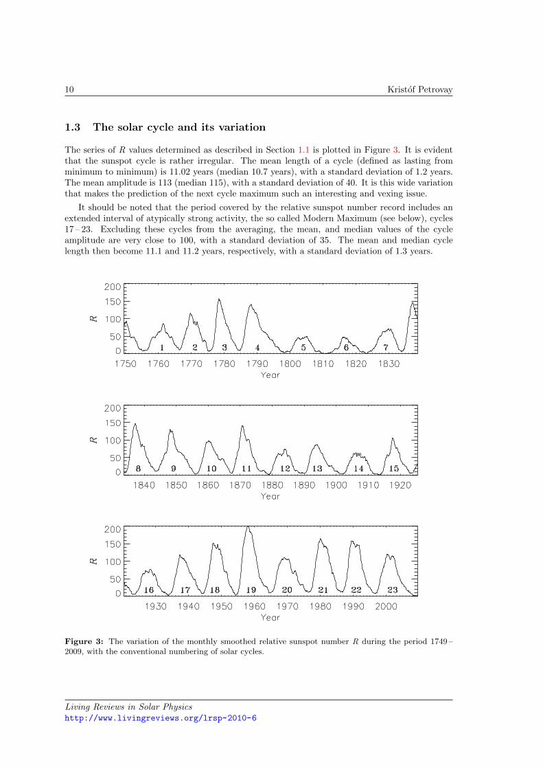
The series of R values determined as described in Section 1.1 is plotted in Figure 3. It is evidentthat the sunspot cycle is rather irregular. The mean length of a cycle (defined as lasting fromminimum to minimum) is 11.02 years (median 10.7 years), with a standard deviation of 1.2 years.The mean amplitude is 113 (median 115), with a standard deviation of 40. It is this wide variationthat makes the prediction of the next cycle maximum such an interesting and vexing issue.

It should be noted that the period covered by the relative sunspot number record includes anextended interval of atypically strong activity, the so called Modern Maximum (see below), cycles17 – 23. Excluding these cycles from the averaging, the mean, and median values of the cycleamplitude are very close to 100, with a standard deviation of 35. The mean and median cyclelength then become 11.1 and 11.2 years, respectively, with a standard deviation of 1.3 years.

Figure 3: The variation of the monthly smoothed relative sunspot number R during the period 1749 –2009, with the conventional numbering of solar cycles.




1.3.1 Secular activity variations

Inspecting Figure 3 one can discern an obvious long term variation. For the study of such longterm variations, the series of cycle parameters is often smoothed on time scales significantly longerthan a solar cycle: this procedure is known as secular smoothing. One popular method is theso-called Gleissberg filter or 12221 filter (Gleissberg, 1967). For instance, the Gleissberg filteredamplitude of cycle n is given by

〈Rmax〉(n)G =1

8

(R(n−2)

max + 2R(n−1)max + 2R(n)

max + 2R(n+1)max +R(n+2)

max

). (4)

Figure 4: Amplitudes of the sunspot cycles (dotted) and their Gleissberg filtered values (blue solid),plotted against cycle number.

The Gleissberg filtered sunspot number series is plotted in Figure 4. One long-term trend is anoverall secular increase of solar activity, the last six or seven cycles being unusually strong. (Fourof them are markedly stronger than average and none is weaker than average.) This period ofelevated sunspot activity level from the mid-20th century is known as the “Modern Maximum”.On the other hand, cycles 5, 6, and 7 are unusually weak, forming the so-called “Dalton Minimum”.Finally, the rather long series of moderately weak cycles 12 – 16 is occasionally referred to as the“Gleissberg Minimum” – but note that most of these cycles are less than 1σ below the long-termaverage.

While the Dalton and Gleissberg minima are but local minima in the ever changing Gleissbergfiltered SSN series, the conspicuous lack of sunspots in the period 1640 – 1705, known as theMaunder Minimum (Figure 1) quite obviously represents a qualitatively different state of solaractivity. Such extended periods of high and low activity are usually referred to as grand maximaand grand minima. Clearly, in comparison with the Maunder Minimum, the Dalton Minimum couldonly be called a “semi-grand minimum”, while for the Gleissberg Minimum even that adjective isundeserved.

A number of possibilities have been proposed to explain the phenomenon of grand minima andmaxima, including chaotic behaviour of the nonlinear solar dynamo (Weiss et al., 1984), stochastic



12 Kristof Petrovay

fluctuations in dynamo parameters (Moss et al., 2008; Usoskin et al., 2009b) or a bimodal dynamowith stochastically induced alternation between two stationary states (Petrovay, 2007).

The analysis of long-term proxy data, extending over several millennia further showed thatthere exist systematic long-term statistical trends and periods such as the so called secular andsupersecular cycles (see Section 3.2).

1.3.2 Does the Sun have a long term memory?

Following customary usage, by “memory” we will refer to some physical (or, in the case of a model,mathematical) mechanism by which the state of a system at a given time will depend on its previousstates. In any system there may be several different such mechanisms at work simultaneously –if this is so, again following common usage we will speak of different “types” of memory. A verymundane example are the RAM and the hard disk in a computer: devices that store informationover very different time scales and the effect of which manifests itself differently in the functioningof the system.

There is no question that the solar dynamo (i.e., the mechanism that gives rise to the sunspotnumber series) does possess a memory that extends at least over the course of a single solar cycle.Obviously, during the rise phase solar activity “remembers” that it should keep growing, while inthe decay phase it keeps decaying, even though exactly the same range of R values are observed inboth phases. Furthermore, profiles of individual sunspot cycles may, in a first approximation, beconsidered a one-parameter ensemble (Hathaway et al., 1994). This obvious effect will be referredto here as intracycle memory.

As we will see, correlations between activity parameters in different cycles are generally muchweaker than those within one cycle, which strongly suggests that the intracycle memory mechanismis different from longer term memory effects, if such are present at all. Referring back to ouranalogy, the intracycle memory may work like computer RAM, periodically erased at every reboot(i.e., at the start of a new cycle).

The interesting question is whether, in addition to the intracycle memory effect, any other typeof memory is present in the solar dynamo or not. To what extent is the amplitude of a sunspotcycle determined by previous cycles? Are subsequent cycles essentially independent, randomlydrawn from some stochastic distribution of cycle amplitudes around the long term average? Or,in the alternative case, for how many previous cycles do we need to consider solar activity forsuccessful forecasts?

The existence of long lasting grand minima and maxima suggests that the sunspot numberrecord must have a long-term memory extending over several consecutive cycles. Indeed, elemen-tary combinatorical calculations show that the occurrence of phenomena like the Dalton minimum(3 of the 4 lowest maxima occurring in a row) or the Modern maximum (4 of the 5 highest max-ima occurring within a series of 5 cycles) in a random series of 24 recorded solar maxima has arather low probability (5% and 3%, respectively). This conclusion is corroborated by the analysisof long-term proxy data, extending over several millennia, which showed that the occurrence ofgrand minima and grand maxima is more common than what would follow from Gaussian statistics(Usoskin et al., 2007).

It could be objected that for sustained grand minima or maxima a memory extending only fromone cycle to the next would suffice. In contrast to long-term (multidecadal or longer) memory, thiswould constitute another kind of short-term (. 10 years) memory: a cycle-to-cycle or intercyclememory effect. In our computer analogy, think of system files or memory cache written on the harddisk, often with the explicit goal of recalling the system status (e.g., desktop arrangement) afterthe next reboot. While these files survive the reboot, they are subject to erasing and rewriting inevery session, so they have a much more temporary character than the generic data files stored onthe disk.




The intercycle memory explanation of persistent secular activity minima and maxima, however,would imply a good correlation between the amplitudes of subsequent cycles, which is not the case(cf. Section 2.1 below). With the known poor cycle-to-cycle correlation, strong deviations fromthe long-term mean would be expected to be damped on time scales short compared to, e.g., thelength of the Maunder minimum. This suggests that the persistent states of low or high activityare due to truly long term memory effects extending over several cycles.

Further evidence for a long-term memory in solar activity comes from the persistence analysisof activity indicators. The parameter determined in such studies is the Hurst exponent 0 < H < 1.Essentially, H is the steepness of the growth of the total range R of measured values plottedagainst the number n of data in a time series, on a logarithmic plot: R ∝ nH . For a Markovianrandom process with no memory H = 0.5. Processes with H > 0.5 are persistent (they tend tostay in a stronger-than-average or weaker-than-average state longer), while those with H < 0.5 areanti-persistent (their fluctuations will change sign more often).

Hurst exponents for solar activity indices have been derived using rescaled range analysis bymany authors (Mandelbrot and Wallis, 1969; Ruzmaikin et al., 1994; Komm, 1995; Oliver andBallester, 1996; Kilcik et al., 2009). All studies coherently yield a value H = 0.85 – 0.88 for timescales exceeding a year or so, and somewhat lower values (H ∼ 0.75) on shorter time scales. Somedoubts regarding the significance of this result for a finite series have been raised by Oliver andBallester (1998); however, Qian and Rasheed (2004) have shown using Monte Carlo experimentsthat for time series of a length comparable to the sunspot record, H values exceeding 0.7 arestatistically significant.

A complementary method, essentially equivalent to rescaled range analysis is detrended fluc-tuation analysis. Its application to solar data (Ogurtsov, 2004) has yielded results in accordancewith the H values quoted above.

The overwhelming evidence for the persistent character of solar activity and for the intermittentappearance of secular cyclicities, however, is not much help when it comes to cycle-to-cycle predic-tion. It is certainly reassuring to know that forecasting is not a completely idle enterprise (whichwould be the case for a purely Markovian process), and the long-term persistence and trends maymake our predictions statistically somewhat different from just the long-term average. There are,however, large decadal scale fluctuations superposed on the long term trends, so the associatederrors will still be so large as to make the forecast of little use for individual cycles.



14 Kristof Petrovay

1.3.3 Waldmeier effect and amplitude–frequency correlation

“Greater activity on the Sun goes with shorter periods, and less with longerperiods. I believe this law to be one of the most important relations among theSolar actions yet discovered.”

(Wolf, 1861)

It is apparent from Figure 3 that the profile of sunspot cycles is asymmetrical, the rise beingsteeper than the decay. Solar activity maxima occur 3 to 4 years after the minimum, while ittakes another 7 – 8 years to reach the next minimum. It can also be noticed that the degree of thisasymmetry correlates with the amplitude of the cycle: to be more specific, the length of the risephase anticorrelates with the maximal value of R (Figure 5), while the length of the decay phaseshows weak or no such correlation.

Historically, the relation was first formulated by Waldmeier (1935) as an inverse correlationbetween the rise time and the cycle amplitude; however, as shown by Tritakis (1982), the totalrise time is a weak (inverse logarithmic) function of the rise rate, so this representation makesthe correlation appear less robust. (Indeed, when formulated with the rise time it is not evenpresent in some activity indicators, such as sunspot areas – cf. Dikpati et al., 2008b.) As pointedout by Cameron and Schussler (2008), the weak link between rise time and slope is due to thefact that in steeper rising cycles the minimum will occur earlier, thus partially compensating forthe shortening due to a higher rise rate. The effect is indeed more clearly seen when the rateof the rise is used instead of the rise time (Lantos, 2000; Cameron and Schussler, 2008). Theobserved correlation between rise rate and maximum cycle amplitude is approximately linear,good (correlation coefficient r ∼ 0.85), and quite robust, being present in various activity indices.

Figure 5: Monthly smoothed sunspot number R at cycle maximum plotted against the rise time tomaximum (left) and against cycle length (right). Cycles are labeled with their numbers. In the plotsthe red dashed lines are linear regressions to all the data, while the blue solid lines are fits to all dataexcept outliers. Cycle 19 is considered an outlier on both plots, cycle 4 on the right hand plot only. Thecorresponding correlation coefficients are shown.




Nevertheless, when coupled with the nearly nonexistent correlation between the decay time andthe cycle amplitude, even the weaker link between the rise time and the maximum amplitude issufficient to forge a weak inverse correlation between the total cycle length and the cycle amplitude(Figure 5). This inverse relationship was first noticed by Wolf (1861).

A stronger inverse correlation was found between the cycle amplitude and the length of theprevious cycle by Hathaway et al. (1994). This correlation is also readily explained as a consequenceof the Waldmeier effect, as demonstrated in a simple model by Cameron and Schussler (2007).Note that in a more detailed study Solanki et al. (2002) find that the correlation coefficient of thisrelationship has steadily decreased during the course of the historical sunspot number record, whilethe correlation between cycle amplitude and the length of the third preceding cycle has steadilyincreased. The physical significance (if any) of this latter result is unclear.

In what follows, the relationships found by Wolf (1861), Hathaway et al. (1994), and Solankiet al. (2002), discussed above, will be referred to as “Rmax – tcycle,n correlations” with n = 0, –1or –3, respectively.

Modern time series analysis methods offer several ways to define an instantaneous frequency f ina quasiperiodic series. One simple approach was discussed in the context of Bracewell’s transform,Equation (3), above. Mininni et al. (2000) discuss several more sophisticated methods to do this,concluding that Gabor’s analytic signal approach yields the best performance. This technique wasfirst applied to the sunspot record by Palus and Novotna (1999), who found a significant long termcorrelation between the smoothed instantaneous frequency and amplitude of the signal. On timescales shorter than the cycle length, however, the frequency–amplitude correlation has not beenconvincingly proven, and the fact that the correlation coefficient is close to the one reported inthe right hand panel of Figure 5 indicates that all the fashionable gadgetry of nonlinear dynamicscould achieve was to recover the effect already known to Wolf. It is clear from this that the“frequency–amplitude correlation” is but a secondary consequence of the Waldmeier effect.

On the left hand panel of Figure 5, within the band of correlation the points seem to besitting neatly on two parallel strings. Any number of faint hearted researchers would dismiss thisas a coincidence or as another manifestation of the “Martian canal effect”. But Kuklin (1986)boldly speculated that the phenomenon may be real. Fair enough, cycles 22 and 23 dutifully tooktheir place on the lower string even after the publication of Kuklin’s work. This speculation wassupported with further evidence by Nagovitsyn (1997) who offered a physical explanation in termsof the amplitude–frequency diagram of a forced nonlinear oscillator (cf. Section 4.5).

Indeed, an anticorrelation between cycle length and amplitude is characteristic of a class ofstochastically forced nonlinear oscillators and it may also be reproduced by introducing a stochasticforcing in dynamo models (Stix, 1972; Ossendrijver et al., 1996; Charbonneau and Dikpati, 2000).In some such models the characteristic asymmetric profile of the cycle is also well reproduced(Mininni et al., 2000, 2002). The predicted amplitude–frequency relation has the form

logR(n)max = C1 + C2f . (5)

Nonlinear dynamo models including some form of α-quenching also have the potential to re-produce the effects described by Wolf and Waldmeier without recourse to stochastic driving. Ina dynamo with a Kleeorin–Ruzmaikin type feedback on α, Kitiashvili and Kosovichev (2009) areable to qualitatively reproduce the Waldmeier effect. Assuming that the sunspot number is relatedto the toroidal field strength according to the Bracewell transform, Equation (3), they find a stronglink between rise time and amplitude, while the correlations with fall time and cycle length aremuch weaker, just as the observations suggest. They also find that the form of the growth time–amplitude relationship differs in the regular (multiperiodic) and chaotic regimes. In the regularregime the plotted relationship suggests

R(n)max = C1 − C2

(t(n)max − t

(n)min

), (6)



16 Kristof Petrovay

while in the chaotic caseR(n)

max ∝[1/(t(n)max − t

(n)min

)]. (7)

Note that based on the actual sunspot number series Waldmeier originally proposed

logR(n)max = C1 − C2

(t(n)max − t

(n)min

), (8)

while according to Dmitrieva et al. (2000) the relation takes the form

logR(n)max ∝

[1/(t(n)max − t

(n)min

)]. (9)

At first glance, these logarithmic empirical relationships seem to be more compatible withthe relation (5) predicted by the stochastic models. These, on the other hand, do not actuallyreproduce the Waldmeier effect, just a general asymmetric profile and an amplitude–frequencycorrelation. At the same time, inspection of the the left hand panel in Figure 5 shows that thedata is actually not incompatible with a linear or inverse rise time–amplitude relation, especially ifthe anomalous cycle 19 is ignored as an outlier. (Indeed, a logarithmic representation is found notto improve the correlation coefficient – its only advantage is that cycle 19 ceases to be an outlier.)All this indicates that nonlinear dynamo models may have the potential to provide a satisfactoryquantitative explanation of the Waldmeier effect, but more extensive comparisons will need to bedone, using various models and various representations of the relation.




2 Precursor Methods

“Jeder Fleckenzyklus muß als ein abgeschlossenes Ganzes, als ein Phanomenfur sich, aufgefaßt werden, und es reiht sich einfach Zyklus an Zyklus.”

(Gleissberg, 1952)

In the most general sense, precursor methods rely on the value of some measure of solar ac-tivity or magnetism at a specified time to predict the amplitude of the following solar maximum.The precursor may be any proxy of solar activity or other indicator of solar and interplanetarymagnetism. Specifically, the precursor may also be the value of the sunspot number at a giventime.

In principle, precursors might also herald the activity level at other phases of the sunspot cycle,in particular the minimum. Yet the fact that practically all the good precursors found need to beevaluated at around the time of the minimum and refer to the next maximum is not simply due tothe obvious greater interest in predicting maxima than predicting minima. Correlations betweenminimum parameters and previous values of solar indices have been looked for, but the resultswere overwhelmingly negative (e.g., Tlatov, 2009). This indicates that the sunspot number seriesis not homogeneous and Rudolf Wolf’s instinctive choice to start new cycles with the minimumrather than the maximum in his numbering system is not arbitrary – for which even more obviousevidence is provided by the butterfly diagram. Each numbered solar cycle is a consistent unit initself, while solar activity seems to consist of a series of much less tightly intercorrelated individualcycles, as suggested by Wolfgang Gleissberg in the motto of this section.

In Section 1.3.2 we have seen that there is significant evidence for a long-term memory under-lying solar activity. In addition to the evidence reviewed there, systematic long-term statisticaltrends and periods of solar activity, such as the secular and supersecular cycles (to be discussed inSection 3.2), also attest to a secular mechanism underlying solar activity variations and ensuringsome degree of long-term coherence in activity indicators. However, as we noted, this long-termmemory is of limited importance for cycle prediction due to the large, apparently haphazard decadalvariations superimposed on it. What the precursor methods promise is just to find a system inthose haphazard decadal variations – which clearly implies a different type of memory. As wealready mentioned in Section 1.3.2, there is obvious evidence for an intracycle memory operatingwithin a single cycle, so that forecasting of activity in an ongoing cycle is currently a much moresuccessful enterprise than cycle-to-cycle forecasting. As we will see, this intracycle memory is onecandidate mechanism upon which precursor techniques may be founded, via the Waldmeier effect.

The controversial issue is whether, in addition to the intracycle memory, there is also an intercy-cle memory at work, i.e., whether behind the apparent stochasticity of the cycle-to-cycle variationsthere is some predictable pattern, whether some imprint of these variations is somehow inheritedfrom one cycle to the next, or individual cycles are essentially independent. The latter is knownas the “outburst hypothesis”: consecutive cycles would then represent a series of “outbursts” ofactivity with stochastically fluctuating amplitudes (Halm, 1901; Waldmeier, 1935; Vitinsky, 1973;see also de Meyer, 1981 who calls this “impulse model”). Note that cycle-to-cycle predictions inthe strict temporal sense may be possible even in the outburst case, as solar cycles are known tooverlap. Active regions belonging to the old and new cycles may coexist for up to three years orso around sunspot minima; and high latitude ephemeral active regions oriented according to thenext cycle appear as early as 2 – 3 years after the maximum (Tlatov et al., 2010 – the so-calledextended solar cycle).

In any case, it is undeniable that for cycle-to-cycle predictions, which are our main concernhere, the precursor approach seems to have been the relatively most successful, so its inherentbasic assumption must contain an element of truth – whether its predictive skill is due to a “real”cycle-to-cycle memory (intercycle memory) or just to the overlap effect (intracycle memory).



18 Kristof Petrovay

The two precursor types that have received most attention are polar field precursors and geo-magnetic precursors. A link between these two categories is forged by a third group, characterizingthe interplanetary magnetic field strength or “open flux”. But before considering these approaches,we start by discussing the most obvious precursor type: the level of solar activity at some epochbefore the next maximum.

2.1 Cycle parameters as precursors and the Waldmeier effect

The simplest weather forecast method is saying that “tomorrow the weather will be just liketoday” (works in about 2/3 of the cases). Similarly, a simple approach of sunspot cycle predictionis correlating the amplitudes of consecutive cycles. There is indeed a marginal correlation, butthe correlation coefficient is quite low (0.35). The existence of the correlation is related to secularvariations in solar activity, while its weakness is due to the significant cycle-to-cycle variations.

A significantly better correlation exists between the minimum activity level and the amplitudeof the next maximum (Figure 6). The relation is linear (Brown, 1976), with a correlation coefficientof 0.72 (if the anomalous cycle 19 is ignored – Brajsa et al., 2009; see also Pishkalo, 2008). Thebest fit is

Rmax = 67.5 + 6.91Rmin . (10)

Using the observed value 1.7 for the SSN in the recent minimum, the next maximum is predictedby this “minimax” method to reach values around 80, with a 1σ error of about ± 25.

Figure 6: Monthly smoothed sunspot number R at cycle maximum plotted against the values of R at theprevious minimum (left) and 2.5 years before the minimum (right). Cycles are labeled with their numbers.The blue solid line is a linear regression to the data; corresponding correlation coefficients are shown. Inthe left hand panel, cycle 19 was considered an outlier.

Cameron and Schussler (2007) point out that the activity level three years before the minimumis an even better predictor of the next maximum. Indeed, playing with the value of time shift wefind that the best correlation coefficient corresponds to a time shift of 2.5 years, as shown in theright hand panel of Figure 6 (but this may depend on the particular time period considered, so we




will refer to this method in Table 1 as “minimax3” for brevity). The linear regression is

Rmax = 41.9 + 1.68R(tmin − 2.5). (11)

For cycle 24 the value of the predictor is 16.3, so this indicates an amplitude of 69, suggesting thatthe upcoming cycle may be comparable in strength to those during the Gleissberg minimum at theturn of the 19th and 20th centuries.

As the epoch of the minimum of R cannot be known with certainty until about a year afterthe minimum, the practical use of these methods is rather limited: a prediction will only becomeavailable 2 – 3 years before the maximum, and even then with the rather low reliability reflected inthe correlation coefficients quoted above. In addition, as convincingly demonstrated by Cameronand Schussler (2007) in a Monte Carlo simulation, these methods do not constitute real cycle-to-cycle prediction in the physical sense: instead, they are due to a combination of the overlap of solarcycles with the Waldmeier effect. As stronger cycles are characterized by a steeper rise phase, theminimum before such cycles will take place earlier, when the activity from the previous cycle hasnot yet reached very low levels.

The same overlap readily explains the Rmax – tcycle,n correlations discussed in Section 1.3.3.These relationships may also be used for solar cycle prediction purposes (e.g., Kane, 2008) butthey lack robustness. For cycle 24 the Rmax – tcycle,−1 correlation, as formulated by Hathaway(2010b) predicts Rmax = 80 while the methods used by Solanki et al. (2002) yield values rangingfrom 86 to about 110, depending on the relative weights of tcycle,−1 and tcycle,−3. The forecastis not only sensitive to the value of n used but also to the data set (relative or group sunspotnumbers) (Vaquero and Trigo, 2008).

2.2 Polar precursors

Direct measurements of the magnetic field in the polar areas of the Sun have been availablefrom Wilcox Observatory since 1976 (Svalgaard et al., 1978; Hoeksema, 1995). Even before asignificant amount of data had been available for statistical analysis, solely on the basis of theBabcock–Leighton scenario of the origin of the solar cycle, Schatten et al. (1978) suggested thatthe polar field measurements may be used to predict the amplitude of the next solar cycle. Datacollected in the four subsequent solar cycles have indeed confirmed this suggestion. As it wasoriginally motivated by theoretical considerations, this polar field precursor method might also bea considered a model-based prediction technique. As, however, no particular detailed mathematicalmodel is underlying the method, numerical predictions must still be based on empirical correlations– hence our categorization of this technique as a precursor method.

The shortness of the available direct measurement series represents a difficulty when it comes tofinding empirical correlations to solar activity. This problem can to some extent be circumventedby the use of proxy data. For instance, Obridko and Shelting (2008) use Hα synoptic mapsto reconstruct the polar field strength at the source surface back to 1915. Spherical harmonicexpansions of global photospheric magnetic measurements can also be used to deduce the fieldstrength near the poles. The use of such proxy techniques permits a forecast with a sufficientlyrestricted error bar to be made, despite the shortness of the direct polar field data set.

The polar fields reach their maximal amplitude near minima of the sunspot cycle. In its mostcommonly used form, the polar field precursor method employs the value of the polar magneticfield strength (typically, the absolute value of the mean field strength poleward of 55° latitudes,averaged for the two hemispheres) at the time of sunspot minimum. It is indeed remarkable thatdespite the very limited available experience, forecasts using the polar field method have provento be consistently in the right range for cycles 21, 22, and 23 (Schatten and Sofia, 1987; Schattenet al., 1996).



20 Kristof Petrovay

Figure 7: Magnetic field strength in the Sun’s polar regions as a function of time. Blue solid: North;red dashed: (−1)·South; thin black solid: average; heavy black solid: smoothed average. Strong annualmodulations in the hemispheric data are due to the tilt of the solar equator to the Ecliptic. Data andfigure courtesy of Wilcox Solar Observatory (see http://wso.stanford.edu/gifs/Polar.gif for updatedversion).


http://wso.stanford.edu/gifs/Polar.gif



By virtue of the definition (2), the time of the minimum of R cannot be known earlier than6 months after the minimum – indeed, to make sure that the perceived minimum was more thanjust a local dip in R, at least a year or so needs to elapse. This would suggest that the predictivevalue of polar field measurements is limited, the prediction becoming available 2 – 3 years beforethe upcoming maximum only.

To remedy this situation, Schatten and Pesnell (1993) introduced a new activity index, the“Solar Dynamo Amplitude” (SoDA) index, combining the polar field strength with a traditionalactivity indicator (the 10.7 cm radio flux F10.7). Around minimum, SoDA is basically proportionalto the polar precursor and its value yields the prediction for F10.7 at the next maximum; however,it was constructed so that its 11-year modulation is minimized, so theoretically it should be ratherstable, making predictions possible well before the minimum. That is the theory, anyway – inreality, SoDA based forecasts made more than 2 – 3 years before the minimum usually provedunreliable. It is then questionable to what extent SoDA improves the prediction skill of the polarprecursor, to which it is more or less equivalent in those late phases of the solar cycle when forecastsstart to become reliable.

Fortunately, however, the maxima of the polar field curves are often rather flat (see Figure 7),so approximate forecasts are feasible several years before the actual minimum. Using the current,rather flat and low maximum in polar field strength, Svalgaard et al. (2005) have been able topredict a relatively weak cycle 24 (peak R value 75 ± 8) as early as 4 years before the sunspotminimum took place in December 2008! Such an early prediction is not always possible: early polarfield predictions of cycles 22 and 23 had to be corrected later and only forecasts made shortly beforethe actual minimum did finally converge. Nevertheless, even the moderate success rate of suchearly predictions seems to indicate that the suggested physical link between the precursor and thecycle amplitude is real.

In addition to their above mentioned use in reconstructing the polar field strength, variousproxies or alternative indices of the global solar magnetic field during the activity minimum mayalso be used directly as activity cycle precursors. Hα synoptic charts are now available from variousobservatories from as early as 1870. As Hα filaments lie on the magnetic neutral lines, these mapscan be used to reconstruct the overall topology, if not the detailed map, of the large-scale solarmagnetic field. Tlatov (2009) has shown that several indices of the polar magnetic field during theactivity minimum, determined from these charts, correlate well with the amplitude of the incipientcycle.

High resolution Hinode observations have now demonstrated that the polar magnetic field hasa strongly intermittent structure, being concentrated in intense unipolar tubes that coincide withpolar faculae (Tsuneta et al., 2008). The number of polar faculae should then also be a plausibleproxy of the polar magnetic field strength and a good precursor of the incipient solar cycle aroundthe minimum. This conclusion was indeed confirmed by Li et al. (2002) and, more recently, byTlatov (2009).

These methods offer a prediction over a time span of 3 – 4 years, comparable to the rise time ofthe next cycle. A significantly earlier prediction possibility was, however, suggested by Makarovet al. (1989) and Makarov and Makarova (1996) based on the number of polar faculae observedat Kislovodsk, which was found to predict the next sunspot cycle with a time lag of 5 – 6 years;even short term annual variations or “surges” of sunspot activity were claimed to be discerniblein the polar facular record. This surprising result may be partly due to the fact that Makarovet al. considered all faculae poleward of 50 ° latitude. Bona fide polar faculae, seen on Hinodeimages to be knots of the unipolar field around the poles, are limited to higher latitudes, so thewider sample may consist of a mix of such “real” polar faculae and small bipolar ephemeral activeregions. These latter are known to obey an extended butterfly diagram, as recently confirmed byTlatov et al. (2010): the first bipoles of the new cycle appear at higher latitudes about 4 yearsafter the activity maximum. It is not impossible that these early ephemeral active regions may



22 Kristof Petrovay

be used for prediction purposes (cf. also Badalyan et al., 2001); but whether or not the result ofMakarov et al. (1989) may be attributed to this is doubtful, as Li et al. (2002) find that even usingall polar faculae poleward of 50° from the Mitaka data base, the best autocorrelation still resultswith a time shift of about 4 years only.

Finally, trying to correlate various solar activity parameters, Tlatov (2009) finds this surprisingrelation:

R(n+1)max = C1 + C2R

(n)max

(t(n)rev − t(n)max

), C1 = 83± 11, C2 = 0.09± 0.02 , (12)

where t(n)rev is the epoch of the polarity reversal in cycle n (typically, about a year after t

(n)max). The

origin of this curious relationship is unclear. In any case, the good correlation coefficient (r = 0.86,based on 12 cycles) and the time lag of ∼ 10 years make this relationship quite remarkable. For

cycle 24 this formula predicts R(24)max = 94± 14.

2.3 Geomagnetic and interplanetary precursors

Relations between the cycle related variations of geomagnetic indices and solar activity were notedlong ago. It is, however, important to realize that the overall correlation between geomagneticindices and solar activity, even after 13-month smoothing, is generally far from perfect. This isdue to the fact that the Sun can generate geomagnetic disturbances in two ways:

(a) By material ejections (such as CMEs or flare particles) hitting the terrestrial magnetosphere.This effect is obviously well correlated with solar activity, with no time delay, so this con-tribution to geomagnetic disturbances peaks near, or a few years after, sunspot maximum.(Note that the occurrence of the largest flares and CMEs is known to peak some years afterthe sunspot maximum – see Figure 16 in Hathaway, 2010b.)

(b) By a variation of the strength of the general interplanetary magnetic field and of solar windspeed. Geomagnetic disturbances may be triggered by the alternation of the Earth’s crossingof interplanetary sector boundaries (slow solar wind regime) and its crossing of high speedsolar wind streams while well within a sector. The amplitude of such disturbances will clearlybe higher for stronger magnetic fields. The overall strength of the interplanetary magneticfield, in turn, depends mainly on the total flux present in coronal holes, as calculated frompotential field source surface models of the coronal magnetic field. At times of low solaractivity the dominant contribution to this flux comes from the two extended polar coronalholes, hence, in a simplistic formulation this interplanetary contribution may be consideredlinked to the polar magnetic fields of the Sun, which in turn is a plausible precursor candidateas we have seen in the previous subsection. As the polar field reverses shortly after sunspotmaximum, this second contribution often introduces a characteristic secondary minimum inthe cycle variation of geomagnetic indices, somewhere around the maximum of the curve.

The component (a) of the geomagnetic variations actually follows sunspot activity with avariable time delay. Thus a geomagnetic precursor based on features of the cycle dominated bythis component has relatively little practical utility. This would seem to be the case, e.g., with theforecast method first proposed by Ohl (1966), who noticed that the minimum amplitudes of thesmoothed geomagnetic aa index are correlated to the amplitude of the next sunspot cycle (see alsoDu et al., 2009).

An indication that the total geomagnetic activity, resulting from both mechanisms does containuseful information on the expected amplitude of the next solar cycle was given by Thompson (1993),who found that the total number of disturbed days in the geomagnetic field in cycle n is relatedto the sum of the amplitudes of cycles n and n+1 (see also Dabas et al., 2008).




A method for separating component (b) was proposed by Feynman (1982) who correlated theannual aa index with the annual mean sunspot number and found a linear relationship between Rand the minimal value of aa for years with such R values. She interpreted this linear relationshipas representing the component (a) discussed above, while the amount by which aa in a givenyear actually exceeds the value predicted by the linear relation would be the contribution of type(b) (the “interplanetary component”). The interplanetary component usually peaks well ahead ofthe sunspot minimum and the amplitude of the peak seemed to be a good predictor of the nextsunspot maximum. However, it is to be noted that the assumption that the “surplus” contributionto aa originates from the interplanetary component only is likely to be erroneous, especially forstronger cycles. It is known that the number of large solar eruptions shows no unique relation toR: in particular, for R > 100 their frequency may vary by a factor of 3 (see Figure 15 in Hathaway,2010b), so in some years they may well yield a contribution to aa that greatly exceeds the minimumcontribution. A case in point was the “Halloween events” of 2003, that very likely resulted in a largefalse contribution to the derived “interplanetary” aa index (Hathaway, 2010a). As a result, thegeomagnetic precursor method based on the separation of the interplanetary component predictsan unusually strong cycle 24 (Rm ∼ 150), in contrast to most other methods, including Ohl’smethod and the polar field precursor, which suggest a weaker than average cycle (Rm ∼ 80 – 90).

In addition to the problem of neatly separating the interplanetary contribution to geomagneticdisturbances, it is also wrong to assume that this interplanetary contribution is dominated bythe effect of polar magnetic fields at all times during the cycle. Indeed, Wang and Sheeley Jr(2009) point out that the interplanetary magnetic field amplitude at the Ecliptic is related to theequatorial dipole moment of the Sun that does not survive into the next cycle, so despite its morelimited practical use, Ohl’s original method, based on the minima of the aa index is physicallybetter founded, as the polar dipole dominates around the minimum. The total amount of openinterplanetary flux, more closely linked to polar fields, could still be determined from geomagneticactivity if the interplanetary contribution to it is further split into:

(b1) A contribution due to the varying solar wind speed (or to the interplanetary magnetic fieldstrength anticorrelated with it), which in turn reflects the strength of the equatorial dipole.

(b2) Another contribution due to the overall interplanetary field strength or open magnetic flux,which ultimately reflects the axial dipole.

Clearly, if the solar wind speed contribution (b1) could also subtracted, a physically better foundedprediction method should result. While in situ spacecraft measurements for the solar wind speedand the interplanetary magnetic field strength do not have the necessary time coverage, Svalgaardand Cliver (2005, 2007) and Rouillard et al. (2007) devised a method to reconstruct the variationsof both variables from geomagnetic measurements alone. Building on their results, Wang andSheeley Jr (2009) arrive at a prediction of Rm = 97 ± 25 for the maximum amplitude of solarcycle 24. To what extent the effect of the Halloween 2003 events has been removed from thisanalysis is unclear. In any case, the prediction agrees fairly well with that of Bhatt et al. (2009)who, assuming a preliminary minimum time of August 2008 and applying a modified form of Ohl’smethod, predict a cycle maximum in late 2012, with an amplitude of 93 ± 20.

The actual run of cycle 24 will be certainly most revealing from the point of view of thesecomplex interrelationships.

The open magnetic flux can also be derived from the extrapolation of solar magnetograms usinga potential field source surface model. The magnetograms applied for this purpose may be actualobservations or the output from surface flux transport models, using the sunspot distribution(butterfly diagram) and the meridional flow as input. Such models indicate that the observedlatitude independence of the interplanetary field strength (“split monopole” structure) is onlyreproduced if the source surface is far enough (> 10R�) and the potential field model is modified



24 Kristof Petrovay

to take into account the heliospheric current sheet (current sheet source surface model, Schusslerand Baumann, 2006; Jiang et al., 2010a). The extrapolations are generally found to agree wellwith in situ measurements where these are available.

2.4 Flows in the photosphere

In the currently widely popular flux transport dynamo models the strong polar fields prevalentaround sunspot minimum are formed by the advection of following polarity flux from active regionsby the poleward meridional flow. Changes in this flow may thus influence the would-be polar fieldsand thereby may serve as precursors of the upcoming cycle.

Such changes, on the other hand, are also associated with the normal course of the solar activitycycle, the overall flow at mid-latitudes being slower before and during maxima and faster duringthe decay phase. Therefore, it is just the cycle-to-cycle variation in this normal pattern that maybe associated with the activity variations between cycles. In this respect it is of interest to notethat the poleward flow in the late phases of cycle 23 seems to have had an excess speed relative tothe previous cycle (Hathaway and Rightmire, 2010). If this were a latitude-independent amplitudemodulation of the flow, then most flux transport dynamo models would predict a stronger thanaverage polar field at the minimum, contrary to observations. On the other hand, in the surfaceflux transport model of Wang et al. (2009) an increased poleward flow actually results in weakerpolar fields, as it lets less leading polarity flux to diffuse across the equator and cancel there. Asthe recent analysis by Munoz-Jaramillo et al. (2010) has shown, the discrepancy resulted from theneglect of leading polarity flux in the Babcock–Leighton source term in flux transport dynamomodels, and it can be remedied by substituting a pair of opposite polarity flux rings as source terminstead of the α-term. With this correction, 2D flux transport and surface flux transport modelsagree in predicting a weaker polar field for faster meridional flow.

It is known from helioseismology that meridional flow speed fluctuations follow a characteristiclatitudinal pattern associated with torsional oscillations and the butterfly diagram, consisting ofa pair of axisymmetric bands of latitudinal flows converging towards the activity belts, migratingtowards the equator, and accompanied by similar high-latitude poleward branches. This suggestsinterpreting the unusual meridional flow speeds observed during cycle 23 as an increased amplitudeof this migrating modulation, rather than a change in the large-scale flow speed (Cameron andSchussler, 2010). In this case, the flows converging on the activity belts tend to inhibit the transportof following polarities to the poles, again resulting in a lower than usual polar field, as observed(Jiang et al., 2010b; note, however, that Svanda et al., 2007 find no change in the flux transportin areas with increased flows). It is interesting to note that the torsional oscillation pattern, andthus presumably the associated meridional flow modulation pattern, was shown to be fairly wellreproduced by a microquenching mechanism due to magnetic flux emerging in the active belts(Petrovay and Forgacs-Dajka, 2002). Observational support for this notion has been providedby the seismic detection of locally increased flow modulation near active regions (Svanda et al.,2007). This suggests that stronger cycles may be associated with a stronger modulation pattern,introducing a nonlinearity into the flux transport dynamo model, as suggested by Jiang et al.(2010b).

In addition to a variation in the amplitude of migrating flow modulations, their migrationspeed may also influence the cycle. Howe et al. (2009) point out that in the current minimum theequatorward drift of the torsional oscillation shear belt corresponding to the active latitude of thecycle has been slower than in the previous minimum. They suggest that this slowing may explainthe belated start of cycle 24.




3 Extrapolation Methods

In contrast to precursor methods, extrapolation methods only use the time series of sunspot num-bers (or whichever solar activity indicator is considered) but they generally rely on more than oneprevious point to identify trends that can be used to extrapolate the data into the future. Theyare therefore also known as time series analysis or, for historic reasons, regression methods.

A cornerstone of time series analysis is the assumption that the time series is homogeneous,i.e., the mathematical regularities underlying its variations are the same at any point of time.This implies that a forecast for, say, three years ahead has equal chance of success in the rising ordecaying phase of the sunspot cycle, across the maximum or, in particular, across the minimum. Inthis case, distinguishing intracycle and intercycle memory effects, as we did in Sections 1.3.2 and2, would be meaningless. This concept of solar activity variations as a continuous process standsin contrast to that underlying precursor methods, where solar cycles are thought of as individualunits lasting essentially from minimum to minimum, correlations within a cycle being considerablystronger than from one cycle to the next. While, as we have seen, there is significant empiricalevidence for the latter view, the possibility of time homogeneity cannot be discarded out of hand.Firstly, if we consider the time series of global parameters (e.g., amplitudes) of cycles, homogeneitymay indeed be assumed fairly safely. This approach has rarely been used for the directly observedsolar cycles as their number is probably too low for meaningful inferences – but the long data setsfrom cosmogenic radionuclides are excellent candidates for time series analysis.

In addition, there may be good reasons to consider the option of homogeneity of solar activitydata even on the scale of the solar cycle. Indeed, in dynamo models the solar magnetic field simplyoscillates between (weak) poloidal and (strong) toroidal configuration: there is nothing inherentlyspecial about either of the two, i.e., there is no a priori reason to attribute a special significanceto solar minimum. While at first glance the butterfly diagram suggests that starting a new cycleat the minimum is the only meaningful way to do it, there may be equally good arguments forstarting a new cycle at the time of polar reversal. There is, therefore, plenty of motivation to tryand apply standard methods of time series analysis to sunspot data.

Indeed, as the sunspot number series is a uniquely homogeneous and long data set, collectedover centuries and generated in a fairly carefully controlled manner, it has become a favoritetestbed of time series analysis methods and is routinely used in textbooks and monographs forillustration purposes (Box et al., 2008; Wei, 2005; Tong, 1990). This section will summarize thevarious approaches, proceeding, by and large, from the simplest towards the most complex.

3.1 Linear regression

Linear (auto)regression means representing the value of a time series at time t by a linear combi-nation of values at times t−Δt, t− 2Δt, . . ., t− pΔt. Admitting some random error εn, the valueof R in point n is

Rn = R0 +

p∑i=1

cn−iRn−i + εn ,

where p is the order of the autoregression and the ci’s are weight parameters. A further twist onthe model admits a propagation of errors from the previous q points:

Rn = R0 +

p∑i=1

cn−iRn−i + εn +

q∑i=1

dn−iεn−i .

This is known as the ARMA (AutoRegressive Moving Average) model.



26 Kristof Petrovay

Linear regression techniques have been widely used for solar activity prediction during thecourse of an ongoing cycle. Their application for cycle-to-cycle prediction has been less commonand successful (Lomb and Andersen, 1980; Box et al., 2008; Wei, 2005).

Brajsa et al. (2009) applied an ARMA model to the series of annual values of R. A successfulfit was found for p = 6, q = 6. Using this fit, the next solar maximum was predicted to take placearound 2012.0 with an amplitude 90 ± 27, and the following minimum occurring in 2017.

Instead of applying an autoregression model directly to SSN data, Hiremath (2008) applied itto a forced and damped harmonic oscillator model claimed to well represent the SSN series. Thisresulted in a predicted amplitude of 110 ± 10 for solar cycle 24, with the cycle starting in mid-2008and lasting 9.34 years.

3.2 Spectral methods

“...the use of any mathematical algorithm to derive hidden periodicities fromthe data always entails the question as to whether the resulting cycles arenot introduced either by the particular numerical method used or by the timeinterval analyzed.”

(de Meyer, 1981)

Spectral analysis of the sunspot number record is used for prediction under the assumptionthat the main reason of variability in the solar cycle is a long-term modulation due to one or moreperiods.

The usual approach to the problem is the purely formal one of representing the sunspot recordwith the superposition of eigenfunctions forming an orthogonal basis. From a technical point ofview, spectral methods are a complicated form of linear regression. The analysis can be performedby any of the widely used means of harmonic analysis:

(1) Least squares (LS) frequency analysis (sometimes called “Lomb–Scargle periodogram”)consists in finding by trial and error the best fitting sine curve to the data using the least squaresmethod, subtracting it (“prewhitening”), then repeating the procedure until the residuals becomeindistinguishable from white noise. The first serious attempt at sunspot cycle prediction, due toKimura (1913), belonged to this group. The analysis resulted in a large number of peaks withdubious physical significance. The prediction given for the upcoming cycle 15 failed, the forecastedamplitude being ∼ 60 while the cycle actually peaked at 105. However, it is interesting to note thatKimura correctly predicted the long term strengthening of solar activity during the first half of the20th century! LS frequency analysis on sunspot data was also performed by Lomb and Andersen(1980), with similar results for the spectrum.

(2) Fourier analysis is probably the most commonly used method of spectral decompositionin science. It has been applied to sunspot data from the beginning of the 20th century (Turner,1913a,b; Michelson, 1913). Vitinsky (1973) judges Fourier-based forecasts even less reliable thanLS periodogram methods. Indeed, for instance Cole (1973) predicted cycle 21 to have a peakamplitude of 60, while the real value proved to be nearly twice that.

(3) The maximum entropy method (MEM) relies on the Wiener–Khinchin theorem that thepower spectrum is the Fourier transform of the autocorrelation function. Calculating the autocor-relation of a time series for M � N points and extrapolating it further in time in a particular wayto ensure maximal entropy can yield a spectrum that extends to arbitrarily low frequencies despitethe shortness of the data segment considered, and also has the property of being able to reproducesharp spectral features (if such are present in the data in the first place). A good description ofthe method is given by Ables (1974), accompanied with some propaganda for it – see Press et al.(1992) for a more balanced account of its pros and cons. The use of MEM for sunspot number




prediction was pioneered by Currie (1973). Using maximum entropy method combined with mul-tiple regression analysis (MRA) to estimate the amplitudes and phases, Kane (2007) arrived at aprediction of 80 to 101 for the maximum amplitude of cycle 24. It should be noted that the samemethod yielded a prediction (Kane, 1999) for cycle 23 that was far off the mark.

(4) Singular spectrum analysis (SSA) is a relatively novel method for the orthogonal decompo-sition of a time series. While in the methods discussed above the base was fixed (the trigonometricfunctions), SSA allows for the identification of a set of othogonal eigenfunctions that are mostsuitable for the problem. This is done by a principal component analysis of the covariance matrixrik = 〈RiRi+k〉. SSA was first applied to the sunspot record by Rangarajan (1998) who only usedthis method for pre-filtering before the application of MEM. Loskutov et al. (2001) who also give agood description of the method, already made a prediction for cycle 24: a peak amplitude of 117.More recently, the forecast has been corrected slightly downwards to 106 (Kuzanyan et al., 2008).

The dismal performance of spectral predictions with the methods (1) – (3) indicates that thesunpot number series cannot be well represented by the superposition of a limited number of fixedperiodic components. Instead,

� the periods may be time dependent,

� the system may be quasiperiodic, with a significant finite width of the periodic peaks (esp.the 11-year peak),

� there may be non-periodic (i.e., chaotic or stochastic) components in the behaviour of thesystem, manifested as a continuous background in the spectrum.

In practice, all three effects suggested above may play some part. The first mentioned effect,time dependence, may in fact be studied within the framework of spectral analysis. MEM andSSA are intrinsically capable of detecting or representing time dependence in the spectrum, whileLS and Fourier analysis can study time dependence by sliding an appropriate data window acrossthe period covered by observations. If the window is Gaussian with a width proportional to thefrequency we arrive at the popular wavelet analysis. This method was applied to the sunspotnumber series by Ochadlick Jr et al. (1993), Vigouroux and Delachie (1994), Frick et al. (1997),Fligge et al. (1999), and Li et al. (2005) who could confirm the existence and slight variation ofthe 11-year cycle and the Gleissberg-cycle. Recently, Kollath and Olah (2009) called attention to avariety of other generalized time dependent spectral analysis methods, of which the pseudo-Wignertransform yields especially clear details (see Figure 9). The time varying character of the basicperiods makes it difficult to use these results for prediction purposes but they are able to shed somelight on the variation as well as the presistent or intermittent nature of the periods determiningsolar activity.

In summary, it is fair to say that forecasts based on harmonic analysis are notoriously unreliable.The secular variation of the basic periods, obeying as yet unknown rules, would render harmonicanalysis practically useless for the prediction of solar cycles even if solar activity could indeed bedescribed by a superposition of periodic functions. Although they may be potentially useful forvery long term prediction (on centennial scales), when it comes to cycle-to-cycle forecasts the bestwe can hope from spectral studies is apparently an indirect contribution, by constraining dynamomodels with the inambiguously detected periodicities.

In what remains from this subsection, we briefly review what these apparently physically realperiods are and what impact they may have on solar cycle prediction.



28 Kristof Petrovay

3.2.1 The 11-year cycle and its harmonics

As an example of the period spectrum obtained by these methods, in Figure 8 we present the FFTbased power spectrum estimate of the smoothed sunspot number record. Three main features areimmediately noticed:

� The dominant 11-year peak, with its sidelobes and its 5.5-year harmonic.

� The 22-year subharmonic, representing the even–odd rule.

� The significant power present at periods longer than 50 years, associated with the Gleissbergcycle.

The dominant peak in the power spectrum is at ∼ 11 years. Significant power is also presentat the first harmonic of this period, at 5.5 years. This is hardly surprising as the sunspot numbercycles, as presented in Figure 3, have a markedly asymmetrical profile. It is a characteristic ofFourier decomposition that in any periodic series of cycles where the profiles of individual cyclesare non-sinusoidal, all harmonics of the base period will appear in the spectrum.

Figure 8: Power spectrum of the smoothed monthly sunspot number series for the period 1749 – 2008.Solid vertical bars mark the 11-year period, its first harmonic and subharmonic; dashed vertical bars aredrawn at a fiducial period of 14.5 years, its harmonic and subharmonic.

Indeed, were it not for the 13-month smoothing, higher harmonics could also be expected toappear in the power spectrum. It has been proposed (Krivova and Solanki, 2002) that theseharmonics are detected in the sunspot record and that they may be related to the periodicities of∼ 1.3 years intermittently observed in solar wind speed (Richardson et al., 1994; Paularena et al.,1995; Szabo et al., 1995; Mursula and Zieger, 2000; Lockwood, 2001) and in the internal rotationvelocity of the Sun (Howe, 2009, Sect. 10.1). An analoguous intermittent 2.5 year variation inthe solar neutrino flux (Shirai, 2004) may also belong to this group of phenomena. It may beworth noting that, from the other end of the period spectrum, the 154-day Rieger period in solarflare occurrence (Rieger et al., 1984; Bai and Cliver, 1990) has also been tentatively linked to the1.3-year periodicity. Unusually strong excitation of such high harmonics of the Schwabe cycle maypossibly be explained by excitation due to unstable Rossby waves in the tachocline (Zaqarashviliet al., 2010).




The 11-year peak in the power spectrum has substantial width, related to the rather widevariation in cycle lengths in the range 9 – 13 years. Yet Figure 8 seems to suggest the presence ofa well detached second peak in the spectrum at a period of ∼ 14 years. The presence of a distinctpeak at the first harmonic and even at the subharmonic of this period seems to support its reality.Indeed, peaks at around 14 and 7 years were already found by other researchers (e.g., Kimura,1913; Currie, 1973) who suggested that these may be real secondary periods of sunspot activity.

The situation is, however, more prosaic. Constraining the time interval considered to data morerecent than 1850, from which time the sunspot number series is considered to be more reliable,the 14.5-year secondary peak and its harmonics completely disappear. On the other hand, thepower spectrum for the years 1783 – 1835 indicates that the appearance of the 14.5-year secondarypeak in the complete series is almost entirely due to the strong predominance of this period (andits harmonic) in that interval. This interval covers the unusually long cycle 4 and the Daltonminimum, consisting of three consecutive unusually weak cycles, when the “normal” 11-year modeof operation was completely suppressed.

As pointed out by Petrovay (2010), this probably does not imply that the Sun was operating ina different mode during the Dalton minimum, the cycle length being 14.5 years instead of the usual11 years. Instead, the effect may be explained by the well known inverse correlation between cyclelength and amplitude, which in turn is the consequence of the strong inverse correlation betweenrise rate and cycle amplitude (Waldmeier effect), combined with a much weaker or nonexistentcorrelation between decay rate and amplitude (see Section 1.3.3). The cycles around the Daltonminimum, then, seem to lie at the low amplitude (or long period) end of a continuum representingthe well known cycle length–amplitude relation, ultimately explained by the Waldmeier effect.

50100

200SN

1750 1800 1850 1900 1950 2000

0.025

0.050

0.075

0.100

0.125

0.150

0.175

0.200

0.225

time [year]

f [c/y]

Figure 9: Pseudo-Wigner power distribution in the sunspot number record, with time on the abscissaand frequency on the ordinate. The three horizontal bands of high power correspond, from bottom to top,to the Gleissberg cycle, the 11-year cycle and its first harmonic. The sunspot number curve is shown ontop for guidance (figure courtesy of Z. Kollath).



30 Kristof Petrovay

A major consequence of this is that the detailed distribution of peaks varies significantly de-pending on the interval of time considered. Indeed, Kollath and Olah (2009) recently applied timedependent harmonic analysis to the sunspot number series and found that the dominant periodshave shown systematic secular changes during the past 300 years (Figure 9). For instance, thebasic period seems to have shortened from 11 years to 10 years between 1850 and 1950, with somemoderate increase in the last 50 years. (This is consistent with the known anticorrelation betweencycle length and amplitude, cf. Section 1.3.3.)

3.2.2 The even–odd (a.k.a. Gnevyshev–Ohl) rule

A cursory look at Figure 3 shows that solar cycles often follow an alternating pattern of higherand lower maxima. In this apparent pattern, already noticed by the early observers (e.g, Turner,1913c), odd cycles have been typically stronger than even cycles in the last two centuries.

This even–odd rule can be given two interpretations: a “weak” one of a general tendency ofalternation between even and odd cycles in amplitude, or a “strong” one of a specific numericalrelation between the amplitudes of consecutive cycles.

Let us first consider the rule in its weak interpretation. At first sight the rule admits manyexceptions, but the amplitude of solar cycles depends on the particular measuring method used.Exceptions from the even–odd alternation rule become less common if a long term trend (calculatedby applying a 12221 or 121 filter, see Section 1.3.1) is subtracted from the data (Charbonneau,2001), or if integrated cycle amplitudes (sums of annual mean sunspot numbers during the cycle)are used (Gnevyshev and Ohl, 1948).

In fact, as evident from, e.g., the work of Mursula et al. (2001) where cycle amplitudes arebased on group sunspot numbers and the amplitude of a cycle is defined as the sum of the annualGSN value over the course of the cycle, the odd–even alternation may be considered as strictlyvalid with only four exceptions:

� In the pairs 7 – 8 and 17 – 18, odd cycles are followed by stronger even cycles at the end ofDalton minimum and at the beginning of the Modern Maximum. These exceptions could bemade to disappear by the subtraction of the long term trend as suggested by Charbonneau(2001).

� The pair 22 – 23 represents another apparent break of the weak even–odd rule which is noteasily explained away, even though the relative difference is smaller if the Kislovodsk sunspotnumber series is used (Nagovitsyn et al., 2009). The possibility is obviously there that thesubtraction of the long term trend may resolve the problem but we have no way to tell inthe near future.

� Prior to cycle 5, the phase of the alternation was opposite, even cycles being stronger thanodd cycles. As cycle 4 is known to have been anomalously long anyway (the so-called “phasecatastrophe” in the solar cycle, Vitinsky et al., 1986) and its decaying phase is not wellcovered by observations (Vaquero, 2007), this gave rise to the suggestion of a “lost solarcycle” between cycles 4 and 5 (Usoskin et al., 2001; Usoskin and Mursula, 2003). This cycle,however, would have been even more anomalous than cycle 4 and despite intensive searchesin historic data the evidence is still not quite conclusive (Krivova et al., 2002; see, however,Usoskin et al., 2009a).

The issue whether the even–odd rule can go through phase jumps or not is important withrespect to its possible origin. One plausible possibility is that the alternation is due to the super-position of a steady primordial magnetic field component on the oscillatory magnetic field generatedby the dynamo (Levy and Boyer, 1982). In this case, any phase jump in the Gnevyshev–Ohl rule




should imply a phase jump in Hale’s polarity rules, too. Alternatively, persistent even–odd al-ternation may also arise in nonlinear dynamos as a period–2 limit cycle (Durney, 2000); witha stochastic forcing occasional phase jumps are also possible (Charbonneau, 2001; Charbonneauet al., 2007).

While we have no information on this from the 18th century phase jump, we can be certainthat there was no such phase jump in polarities in the last two decades, even though the even–oddrule seems to have been broken again. It will be interesting to see when (and if) the even–odd rulesettles in again, whether it will have done so with a phase jump or not. For instance, if cycle 25 willagain exceed cycle 24 it would seem that no phase jump occurred and both theoretical options arestill open. But if cycle 25 will represent a further weakening from cycle 24, followed by a strongercycle 26, a phase jump will have occurred, which may exclude the primordial field origin of therule if Hale’s polarity rules remain unchanged.

Let us now discuss the stronger interpretation of the even–odd rule. In the first quantitativestudy of the relative amplitudes of consecutive cycles, Gnevyshev and Ohl (1948) found a rathertight correlation between the time integrated amplitudes of even and subsequent odd cycles, whilethe correlation between odd cycles and subsequent even cycles was found to be much less strong.This gave rise to the notion that solar cycles come in “two-packs” as even–odd pairs. Nagovitsynet al. (2009) confirmed this puzzling finding on the basis of data covering the whole period oftelescopic observations (and renumbering cycles before 1790 in accordance with the lost cyclehypothesis); they also argue that cycle pair 22 – 23 does not deviate strongly from the even–oddcorrelation curve so it should not be considered a “real” exception to the even–odd rule.

The fact that shortly after its formulation by Gnevyshev and Ohl (1948), the (strong) even–oddrule was used by Kopecky (1950) to successfully predict the unusually strong cycle 19 made thismethod particularly popular for forecast purposes. However, forecasts based on the even–odd rulecompletely failed for cycle 23, overpredicting the amplitude by > 50% (see review by Li et al.,2001). Taken together with the implausibility of the suggested two-pack system, this shows thatit is probably wiser to take the position that “extraordinary claims need extraordinary evidence”– which is yet to be provided in the case of the “strong” even–odd rule.

Finally, in the context of the even–odd rule, it is also worth mentioning the three-cycle regularityproposed by Ahluwalia (1998). Even though the evidence presented for the alleged triadic patternis not overwhelming, this method resulted in one of the few successful predictions for the amplitudeof cycle 23.

3.2.3 The Gleissberg cycle

Besides the changes in the length of the 11-year cycle related to the amplitude–cycle length cor-relation, even more significant are the variations in the period of the so-called Gleissberg cycle(Gleissberg, 1939). This “cycle”, corresponding to the 60 – 120 year “plateau” in Figure 8 wasactually first noticed by Wolf, who placed it in the range 55 – 80 years (see Richard, 2004, fora discussion of the history of the studies of the Gleissberg cycle). Researchers in the middle ofthe 20th century characterized it as an 80 – 100 year variation. Figure 9 explains why so widelydiffering periods were found in different studies: the period has in fact shown a secular increase inthe past 300 years, from about 50 years in the early 18th century, to a current value exceeding 140years. This increased length of the Gleissberg cycle also agrees with the results of Forgacs-Dajkaand Borkovits (2007).

The detection of ∼ 100 year periods in a data set of 300 years is of course always questionable,especially if the period is even claimed to be varying. However, the very clear and, most impor-tantly, nearly linear secular trend seen in Figure 9 argues convincingly for the reality of the periodin question. This clear appearance of the period is due to the carefully optimized choice of thekernel function in the time–frequency analysis, a method resulting in a so-called pseudo-Wigner



32 Kristof Petrovay

distribution (PWD). In addition, in their study Kollath and Olah (2009) present an extremely con-scientious test of the reliability of their methods, effectively proving that the most salient featuresin their PWD are not artefacts. (The method was subsequently also applied to stellar activity,Olah et al., 2009.) This is the most compelling evidence for the reality of the Gleissberg cycle yetpresented.

3.2.4 Supersecular cycles

For the 210-year Suess cycle, McCracken and Beer (2008) present further evidence for the tempo-rally intermittent nature of this marked peak in the spectrum of solar proxies. The Suess cycleseems to have a role in regulating the recurrence rate of grand minima. Grand minima, in turn,only seem to occur during < 1 kiloyear intervals (“Sporer events”) around the minimum of the∼ 2400-year Hallstatt cycle.

For further discussion of long term variations in solar activity we refer the reader to the reviewsby Beer et al. (2006) and Usoskin (2008).




3.3 Nonlinear methods

“...every complicated question has a simple answer which is wrong. Analyzinga time series with a nonlinear approach is definitely a complicated problem.Simple answers have been repeatedly offered in the literature, quoting numer-ical values for attractor dimensions for any conceivable system.”

(Hegger et al., 1999)

The nonlinearities in the dynamo equations readily give rise to chaotic behaviour of the solu-tions. The long term behaviour of solar activity, with phenomena like grand minima and grandmaxima, is also suggestive of a chaotic system. While chaotic systems are inherently unpredictableon long enough time scales, their deterministic nature does admit forecast within a limited range.It is therefore natural to explore this possibility from the point of view of solar cycle prediction.

3.3.1 Attractor analysis and phase space reconstruction: the pros ...

Assuming that the previous (M − 1) values of the sunspot number do in some way determinethe current expected value, our problem becomes restricted to an M -dimensional phase space, thedimensions being the current value and the (M − 1) previous values. With a time series of lengthN , we have N −M + 1 points fixed in the phase space, consecutive points being connected by aline. This phase space trajectory is a sampling of the attractor of the physical system underlyingthe solar cycle (with some random noise added to it). The attractor represents a mapping inphase space which maps each point into the one the system occupies in the next time step: if thismapping is known to a good approximation, it can be used to extend the trajectory towards thefuture.

For the mapping to be known, M needs to be high enough to avoid self-crossings in the phasespace trajectory (otherwise the mapping is not unique) but low enough so that the trajectory stillyields a good sampling of the attractor. The lowest integer dimension satisfying these conditionsis the embedding dimension D of the attractor (which may have a fractal dimension itself).

Once the attractor has been identified, its mathematical description may be done in two ways.(1) Parametric fitting of the attractor mapping in phase space. The simplest method is the

piecewise linear fit suggested by Farmer and Sidorowich (1987) and applied in several solar predic-tion attempts, e.g., Kurths and Ruzmaikin (1990). Using a method belonging to this group, forcycle 24 Kilcik et al. (2009) predict a peak amplitude of 87 to be reached in late 2012. Alterna-tively, a global nonlinear fit can also be used: this is the method applied by Serre and Nesme-Ribes(2000) as the first step in their global flow reconstruction (GFR) approach.

(2) Nonparametric fitting. The simplest nonparametric fit is to find the closest known attractorpoint to ours (in the (M − 1)-dimensional subspace excluding the last value) and then using thisfor a prediction, as done by Jensen (1993). (This resulted in so large random forecast errors that itis practically unsuitable for prediction.) Neural networks, discussed in more detail in Section 3.3.4below, are a much more sophisticated nonparametric fitting device.

(3) Indirectly, one may try to find a set of differential equations describing a system that givesrise to an attractor with properties similar to the observed. In this case there is no guarantee thatthe derived equations will be unique, as an alternative, completely different set may also give rise toa very similar attractor. This arbitrariness of the choice is not necessarily a problem from the pointof view of prediction as it is only the mapping (the attractor structure) that matters. Such phasespace reconstruction by a set of governing equations was performed, e.g., by Serre and Nesme-Ribes(2000) or Aguirre et al. (2008); for cycle 24 the latter authors predict a peak amplitude of 65 ± 16.On the other hand, instead of putting up with any arbitrary set of equations correctly reproducingthe phase space, one might make an effort to find a set with a structure reasonably similar to the



34 Kristof Petrovay

dynamo equations so they can be given a meaningful physical interpretation. Methods followingthis latter approach will be discussed in Sections 4.4 and 4.5.

3.3.2 ... the cons ...

Finding the embedding dimension and the attractor structure is not a trivial task, as shown bythe widely diverging results different researchers arrived at. One way to find the correct embed-ding dimension is the false nearest neighbours method (Kennel et al., 1992), essentially designedto identify self-crossing in the phase space trajectory, in which case the dimension M needs tobe increased. But self-crossings are to some extent inevitable, due to the stochastic componentsuperimposed on the deterministic skeleton of the system.

As a result, the determination of the minimal necessary embedding dimension is usually doneindirectly. One indirect method fairly popular in the solar community is the approach proposed bySugihara and May (1990) where the correct dimension is basically figured out on the basis of howsuccessfully the model, fit to the first part of the data set, can “predict” the second part (using apiecewise linear mapping).

Another widely used approach, due to Grassberger and Procaccia (1983), starts by determiningthe correlation dimension of the attractor, by simply counting how the number of neighbours in anembedding space of dimension M � 1 increases with the distance from a point. If the attractoris a lower dimensional manifold in the embedding space and it is sufficiently densely sampled byour data then the logarithmic steepness d of this function should be constant over a considerablestretch of the curve: this is the correlation dimension d. Now, we can increase M gradually andsee at what value d saturates: that value determines the attractor dimension, while the value ofM where saturation is reached yields the embedding dimension.

The first nonlinear time series studies of solar activity indicators suggested a time series spacingof 2 – 5 years, an attractor dimension ∼ 2 – 3 and an embedding dimension of 3 – 4 (Kurths andRuzmaikin, 1990; Gizzatullina et al., 1990). Other researchers, however, were unable to confirmthese results, either reporting very different values or not finding any evidence for a low dimensionalattractor at all (Calvo et al., 1995; Price et al., 1992; Carbonell et al., 1994; Kilcik et al., 2009;Hanslmeier and Brajsa, 2010). In particular, I would like to call attention to the paper by Jensen(1993), which, according to ADS and WoS, has received a grand total of zero citations (!) upto 2010, yet it displays an exemplary no-nonsense approach to the problem of sunspot numberprediction by nonlinear time series methods. Unlike so many other researchers, the author of thatpaper does not fool himself into believing to see a linear segment on the logarithmic correlationintegral curve (his Figure 4); instead, he demonstrates on a simple example that the actual curvecan be perfectly well reproduced by a simple stochastic process.

These contradictory results obviously do not imply that the mechanism generating solar activityis not chaotic. For a reliable determination a long time series is desirable to ensure a sufficientlylarge number of neighbours in a phase space volume small enough compared to the global scale ofthe attractor. Solar data sets (even the cosmogenic radionuclide proxies extending over millenniabut providing only a decadal sampling) are typically too short and sparse for this. In addition,clearly distinguishing between the phase space fingerprints of chaotic and stochastic processes isan unsolved problem of nonlinear dynamics which is not unique to solar physics. A number ofmethods have been suggested to identify chaos unambiguously in a time series but none of themhas been generally accepted and this topic is currently a subject of ongoing research – see, e.g., thework of Freitas et al. (2009) which demonstrates that the method of “noise titration”, somewhatakin to the Sugihara–May algorithm, is uncapable of distinguishing superimposed coloured noisefrom intrinsically chaotic systems.




3.3.3 ... and the upshot

Starting from the 1980s many researchers jumped on the chaos bandwagon, applying nonlineartime series methods designed for the study of chaotic systems to a wide variety of empirical data,including solar activity parameters. From the 1990s, however, especially after the publication of theinfluential book by Kantz and Schreiber (1997), it was increasingly realized that the applicability ofthese nonlinear algorithms does not in itself prove the predominantly chaotic nature of the systemconsidered. In particular, stochastic noise superposed on a simple, regular, deterministic skeletoncan also give rise to phase space characteristics that are hard to tell from low dimensional chaos,especially if strong smoothing is applied to the data. As a result, the pendulum has swung in theopposite direction and currently the prevailing view is that there is no clear cut evidence for chaosin solar activity data (Panchev and Tsekov, 2007).

One might take the position that any forecast based on attractor analysis is only as good asthe underlying assumption of a chaotic system is: if that assumption is unverifiable from the data,prediction attempts are pointless. This, however, is probably a too hasty judgment. As we willsee, the potentially most useful product of phase space reconstruction attempts is the inferencesthey allow regarding the nature of the underlying physical system (chaotic or not), even offeringa chance to constrain the form of the dynamo equations relevant for the Sun. As discussed inthe next section, such truncated models may be used for forecast directly, or alternatively, theinsight they yield into the mechanisms of the dynamo may be used to construct more sophisticateddynamo models.

3.3.4 Neural networks

Neural networks are algorithms built up from a large number of small interconnected units (“neu-rons” or “threshold logic units”), each of which is only capable of performing a simple nonlinearoperation on an input signal, essentially described by a step function or its generalized (rounded)version, a sigmoid function. To identify the optimal values of thresholds and weights parameteriz-ing the sigmoid functions of each neuron, an algorithm called “back propagation rule” is employedwhich minimizes (with or without human guidance) the error between the predicted and observedvalues in a process called “training” of the network. Once the network has been correctly trained,it is capable of further predictions.

The point is that any arbitrary multidimensional nonlinear mapping may be approximated bya combination of stepfunctions to a good degree – so, as mentioned in Section 3.3.1 above, theneural network can be used to find the nonlinear mapping corresponding to the attractor of thegiven time series.

More detailed introductions to the method are given by Blais and Mertz (2001) and by Calvoet al. (1995); the latter authors were also the first to apply a neural network for sunspot numberprediction. Unfortunately, despite their claim of being able to “predict” (i.e., postdict) some earliercycles correctly, their prediction for cycle 23 was off by a wide margin (predicted peak amplitudeof 166 as opposed to 121 observed). One of the neural network forecasts for cycle 24 (Maris andOncica, 2006) was equally far off, predicting a maximum of 145 as early as December 2009, whileanother one (Uwamahoro et al., 2009) yields a more conservative value of 117.5 ± 8.5 for 2012.



36 Kristof Petrovay

4 Model-Based Predictions

“Progress in dynamo theory is extremely difficult, as it can be made onlyby understanding the interaction of turbulent plasma motions with magneticfields. Indeed, the extreme conditions within the solar interior make this aformidable task. ... Any predictions made with such models should be treatedwith extreme caution (or perhaps disregarded), as they lack solid physical un-derpinnings.”

(Tobias et al., 2006)

While attempts to predict future solar cycles on the basis of the empirical sunspot number recordhave a century-old history, predictions based on physical models of solar activity only started afew years ago. The background of this new trend is, however, not some significant improvementin our understanding of the solar dynamo. Rather, it is the availability of increasingly fast newcomputers that made it possible to fine-tune the parameters of certain dynamo models to reproducethe available sunspot record to a good degree of accuracy and to apply data assimilation methods(such as those used in terrestrial weather prediction) to these models. This is not without perils.On the one hand, the capability of multiparametric models to fit a multitude of observational datadoes not prove the conceptual correctness of the underlying model. On the other hand, in chaoticor stochastic systems such as the solar dynamo, fitting a model to existing data will not lead to agood prediction beyond a certain time span, the extent of which can only be objectively assessed by“postdiction” tests, i.e., checking the models predictive skill by trying to “predict” previous solarcycles and comparing those predictions to available data. Apparently successful postdiction testshave led some groups to claim a breakthrough in solar cycle prediction owing to the model-basedapproach (Dikpati and Gilman, 2006; Kitiashvili and Kosovichev, 2008). Yet, as we will see in thefollowing discussion, a closer inspection of these claims raises many questions regarding the rolethat the reliance on a particular physical dynamo model plays in the success of their predictions.

4.1 The solar dynamo: a brief summary of current models

Extensive summaries of the current standing of solar dynamo theory are given in the reviewsby Petrovay (2000), Ossendrijver (2003), Charbonneau (2010), and Solanki et al. (2006). Asexplained in detail in those reviews, all current models are based on the mean-field theory approachwherein a coupled system of partial differential equations governs the evolution of the toroidal andpoloidal components of the large-scale magnetic field. The large-scale field is assumed to be axiallysymmetric in practically all current models. In some nonlinear models the averaged equation ofmotion, governing large-scale flows is also coupled into the system.

In the simplest case of homogeneous and isotropic turbulence, where the scale l of turbulenceis small compared to the scale L of the mean variables (scale separation hypothesis), the dynamoequations have the form

∂B

∂t= ∇× (U×B+ αB)−∇× (ηT ×∇B) . (13)

Here B and U are the large-scale mean magnetic field and flow speed, respectively; ηT is themagnetic diffusivity (dominated by the turbulent contribution for the highly conductive solarplasma), while α is a parameter related to the non-mirror symmetric character of the magnetizedplasma flow.

In the case of axial symmetry the mean flow U may be split into a meridional circulation Uc

and a differential rotation characterized by the angular velocity profile Ω0(r, θ):

U = Uc + r sin θΩ0 eφ ,




where r, θ, φ are spherical coordinates and eφ is the azimuthal unit vector. Now introducing theshear

Ω = r sin θ∇Ω0, Ω = −sgn dΩ0

dr· |Ω|,

assuming α � ΩL and ignoring spatial derivatives of α and ηT , Equation (13) simplifies to thepair

∂A

∂t= αB − (Uc · ∇)A− (∇ ·Uc)A+ ηT ∇2A , (14)

∂B

∂t= Ω

∂A

∂x− (Uc · ∇)B − (∇ ·Uc)B + ηT ∇2B, (15)

where B and A are the toroidal (azimuthal) components of the magnetic field and of the vector

potential, respectively, and ∂A∂x is to be evaluated in the direction 90° clockwards of ~Ω (along the

isorotation surface) in the meridional plane. These are the classic αΩ dynamo equations, includinga meridional flow.

In the more mainstream solar dynamo models the strong toroidal field is now generally thoughtto reside near the bottom of the solar convective zone. Indeed, it is known that a variety of fluxtransport mechanisms such as pumping (Petrovay, 1994) remove magnetic flux from the solar con-vective zone on a timescale short compared to the solar cycle. Following earlier simpler numericalexperiments, recent MHD numerical simulations have indeed demonstrated this pumping of largescale magnetic flux from the convective zone into the tachocline below, where it forms strongcoherent toroidal fields (Browning et al., 2006). As this layer is also where rotational shear ismaximal, it is plausible that the strong toroidal fields are not just stored but also generated here,by the winding up of poloidal field. The two main groups of dynamo models, interface dynamosand flux transport dynamos, differ mainly in their assumptions about the site and mechanism ofthe α-effect responsible for the generation of a new poloidal field from the toroidal field.

In interface dynamos α is assumed to be concentrated near the bottom of the convective zone,in a region adjacent to the tachocline, so that the dynamo operates as a wave propagating along theinterface between these two layers. While these models may be roughly consistent and convincingfrom the physical point of view, they have only had limited success in reproducing the observedcharacteristics of the solar cycle, such as the butterfly diagram.

Flux transport dynamos, in contrast, rely on the Babcock–Leighton mechanism for α, arisingdue to the action of the Coriolis force on emerging flux loops, and they assume that the corre-sponding α-effect is concentrated near the surface. They keep this surface layer incommunicadowith the tachocline by introducing some arbitrary unphysical assumptions (such as very low diffu-sivities in the bulk of the convective zone). The poloidal fields generated by this surface α-effectare then advected to the poles and there down to the tachocline by the meridional circulation –which, accordingly, has key importance in these models. The equatorward deep return flow ofthe meridional circulation is assumed to have a significant overlap with the tachocline (anothercontroversial point), and it keeps transporting the toroidal field generated by the rotational sheartowards the equator. By the time it reaches lower latitudes, it is amplified sufficiently for theflux emergence process to start, resulting in the formation of active regions and, as a result ofthe Babcock–Leighton mechanism, in the reconstruction of a poloidal field near the surface witha polarity opposed to that in the previous 11-year cycle. While flux transport models may bequestionable from the point of view of their physical consistency, they can be readily fine-tuned toreproduce the observed butterfly diagram quite well.

It should be noted that while the terms “interface dynamo” and “flux transport dynamo” arenow very widely used to describe the two main approaches, the more generic terms “advection-dominated” and “diffusion-dominated” would be preferable in several respects. This classificationallows for a continuous spectrum of models depending on the numerical ratio of advective anddiffusive timescales (for communication between surface and tachocline). In addition, even at



38 Kristof Petrovay

the two extremes, classic interface dynamos and circulation-driven dynamos are just particularexamples of advection or diffusion dominated systems with different geometrical structures.

4.2 Is model-based cycle prediction feasible?

As it can be seen even from the very brief and sketchy presentation given above, all current solardynamo models are based on a number of quite arbitrary assumptions and depend on a number offree parameters, the functional form and amplitude of which is far from being well constrained. Forthis reason, Bushby and Tobias (2007) rightfully say that all current solar dynamo models are onlyof “an illustrative nature”. This would suggest that as far as solar cycle prediction is concerned,the best we should expect from dynamo models is also an “illustrative” reproduction of a seriesof solar cycles with the same kind of long-term variations (qualitatively and, in the statisticalsense, quantitatively) as seen in solar data. Indeed, Bushby and Tobias (2007) demonstratedthat even a minuscule stochastic variation in the parameters of a particular flux transport modelcan lead to large, unpredictable variations in the cycle amplitudes. And even in the absence ofstochastic effects, the chaotic nature of nonlinear dynamo solutions seriously limits the possibilitiesof prediction, as the authors find in a particular interface dynamo model: even if the very samemodel is used to reproduce the results of one particular run, the impossibility of setting initialconditions exactly representing the system implies that predictions are impossible even for thenext cycle. Somewhat better results are achieved by an alternative method, based on the phasespace reconstruction of the attractor of the nonlinear system – this is, however, a purely empiricaltime series analysis technique for which no knowledge of the detailed underlying physics is needed.(Cf. Section 3.3 above.)

Despite these very legitimate doubts regarding the feasibility of model-based prediction of solarcycles, in recent years several groups have claimed to be able to predict solar cycle 24 on the basisof dynamo models with a high confidence. So let us consider these claims.

4.3 Explicit models

The current buzz in the field of model-based solar cycle prediction was started by the work of thesolar dynamo group in Boulder (Dikpati et al., 2006; Dikpati and Gilman, 2006). Their model is aflux transport dynamo, advection-dominated to the extreme. The strong suppression of diffusiveeffects is assured by the very low value (less than 20 km2 s–1) assumed for the turbulent magneticdiffusivity in the bulk of the convective zone. As a result, the poloidal fields generated nearthe surface by the Babcock–Leighton mechanism are only transported to the tachocline on thevery long, decadal time scale of meridional circulation. The strong toroidal flux residing in thelow-latitude tachocline, producing solar activity in a given cycle is thus the product of the shearamplification of poloidal fields formed near the surface about 2 – 3 solar cycles earlier, i.e., themodel has a “memory” extending to several cycles. The mechanism responsible for cycle-to-cyclevariation is assumed to be the stochastic nature of the flux emergence process. In order to representthis variability realistically, the model drops the surface α-term completely (a separate, smallerα term is retained in the tachocline); instead, the generation of poloidal field near the surface isrepresented by a source term, the amplitude of which is based on the sunspot record, while itsdetailed functional form remains fixed.

Dikpati and Gilman (2006) find that, starting off their calculation by fixing the source termamplitudes of sunspot cycles 12 to 15, they can predict the amplitudes of each subsequent cyclewith a reasonable accuracy, provided that the relation between the relative sunspot numbers andthe toroidal flux in the tachocline is linear, and that the observed amplitudes of all previous cyclesare incorporated in the source term for the prediction of any given cycle. For the upcoming cycle 24the model predicts peak smoothed annual relative sunspot numbers of 150 or more. Elaborating




on their model, they proceeded to apply it separately to the northern and southern hemispheres,to find that the model can also be used to correctly forecast the hemispheric asymmetry of solaractivity (Dikpati et al., 2007).

The extraordinary claims of this pioneering research have prompted a hot debate in the dynamocommunity. Besides the more general, fundamental doubt regarding the feasibility of model-basedpredictions (see Section 3.2 above), more technical concerns arose, to be discussed below.

Another flux transport dynamo code, the Surya code, originally developed by A. Choudhuriand coworkers in Bangalore, has also been utilized for prediction purposes. The crucial differencebetween the two models is in the value of the turbulent diffusivity assumed in the convective zone:in the Bangalore model this value is 240 km2 s–1, 1 – 2 orders of magnitude higher than in theBoulder model, and within the physically plausible range (Chatterjee et al., 2004). As a result ofthe shorter diffusive timescale, the model has a shorter memory, not exceeding one solar cycle. Asa consequence of this relatively rapid diffusive communication between surface and tachocline, thepoloidal fields forming near the surface at low latitudes due to the Babcock–Leighton mechanismdiffuse down to the tachocline in about the same time as they reach the poles due to the advectionby the meridional circulation. In these models, then, polar magnetic fields are not a true physicalprecursor of the low-latitude toroidal flux, and their correlation is just due to their common source.In the version of the code adapted for cycle prediction (Choudhuri et al., 2007; Jiang et al., 2007),the “surface” poloidal field (i.e., the poloidal field throughout the outer half of the convectionzone) is rescaled at each minimum by a factor reflecting the observed amplitude of the Sun’s dipolefield. The model shows reasonable predictive skill for the last three cycles for which data areavailable, and can even tackle hemispheric asymmetry (Goel and Choudhuri, 2009). For cycle 24,the predicted amplitude is 30 – 35% lower than cycle 23.

4.4 Truncated models

The “illustrative” nature of solar dynamo models is nowhere more clearly on display than intruncated or reduced models where some or all of the detailed spatial structure of the system iscompletely disregarded, and only temporal variations are explicitly considered. This is sometimesrationalised as a truncation or spatial integration of the equations of a more realistic inhomogenoussystem; in other cases, no such rationalisation is provided, representing the solar dynamo by aninfinite, homogeneous or periodic turbulent medium where the amplitude of the periodic large-scalemagnetic field varies with time only.

In the present subsection we deal with models that do keep one spatial variable (typically, thelatitude), so growing wave solutions are still possible – these models, then, are still dynamos eventhough their spatial structure is not in a good correspondence with that of the solar dynamo.

This approach in fact goes back to the classic migratory dynamo model of Parker (1955) whoradially truncated (i.e., integrated) his equations to simplify the problem. Parker seems to havebeen the first to employ a heuristic relaxation term of the form −Br/τd in the poloidal fieldequation to represent the effect of radial diffusion; here, τd = d2/ηT is the diffusive timescaleacross the thickness d of the convective zone. His model was recently generalized by Moss et al.(2008) and Usoskin et al. (2009b) to the case when the α-effect includes an additive stochasticnoise, and nonlinear saturation of the dynamo is achieved by α-quenching. These authors do notmake an attempt to predict solar activity with their model but they can reasonably well reproducesome features of the very long term solar activity record, as seen from cosmogenic isotope studies.

Another radially truncated model, this time formulated in a Cartesian system, is that of Kiti-ashvili and Kosovichev (2009). In this model stochastic effects are not considered and, in additionto using an α-quenching recipe, further nonlinearity is introduced by coupling in the Kleeorin–Ruzmaikin equation (Zel’dovich et al., 1983) governing the evolution of magnetic helicity, which inthe hydromagnetic case contributes to α. Converting the toroidal field strength to relative sunspot



40 Kristof Petrovay

number using the Bracewell transform, Equation (3), the solutions reproduce the asymmetric pro-file of the sunspot number cycle. For sufficiently high dynamo numbers the solutions becomechaotic, cycle amplitudes show an irregular variation. Cycle amplitudes and minimum–maximumtime delays are found to be related in a way reminiscent of the Waldmeier relation.

Building on these results, Kitiashvili and Kosovichev (2008) attempt to predict solar cyclesusing a data assimilation method. The approach used is the so-called Ensemble Kalman Filtermethod. Applying the model for a “postdiction” of the last 8 solar cycles yielded astonishinglygood results, considering the truncated and arbitrary nature of the model and the fundamentalobstacles in the way of reliable prediction discussed above. While the presently available briefpreliminary publication leaves several details of the method unclear, the question may arise whetherthe actual physics of the model considered has any significant role in this prediction, or we aredealing with something like the phase space reconstruction approach discussed in Section 3.3 abovewhere basically any model with an attractor that looks reasonably similar to that of the actualsolar dynamo would do. Either way, the method is remarkable, and the prediction for cycle 24 of amaximal smoothed annual sunspot number of 80, to be reached in 2013, will be worth comparingto the actual value.

In order to understand the origin of the predictive skill of the Boulder model, Cameron andSchussler (2007) studied a radially truncated version of the model, wherein only the equation forthe radial field component is solved as a function of time and latitude. The equation includes asource term similar to the one used in the Boulder model. As the toroidal flux does not figurein this simple model, the authors use the transequatorial flux Φ as a proxy, arguing that thismay be more closely linked to the amplitude of the toroidal field in the upcoming cycle thanthe polar field. They find that Φ indeed correlates quite well (correlation coefficients r ∼ 0.8 – 0.9,depending on model details) with the amplitude of the next cycle, as long as the form of the latitudedependence of the source term is prescribed and only its amplitude is modulated with the observedsunspot number series (“idealized model”). But surprisingly, the predictive skill of the model iscompletely lost if the prescribed form of the source function is dropped and the actually observedlatitude distribution of sunspots is used instead (“realistic model”). Cameron and Schussler (2007)interpret this by pointing out that Φ is mainly determined by the amount of very low latitude fluxemergence, which in turn occurs mainly in the last few years of the cycle in the idealized model,while it has a wider temporal distribution in the realistic model. The conclusion is that the rootof the apparently good predictive skill of the truncated model (and, by inference, of the Bouldermodel it is purported to represent) is actually just the good empirical correlation between late-phase activity and the amplitude of the next cycle, discussed in Section 2.1 above. This correlationis implicitly “imported” into the idealized flux transport model by assuming that the late-phaseactivity is concentrated at low latitudes, and therefore gives rise to cross-equatorial flux whichthen serves as a seed for the toroidal field in the next cycle. So if Cameron and Schussler (2007)are correct, the predictive skill of the Boulder model is due to an empirical precursor and is thusultimately explained by the good old Waldmeier effect (cf. Section 1.3.3)

The fact that the truncated model of Cameron and Schussler (2007) is not identical to the Boul-der model obviously leaves room for doubt regarding this conclusion. In particular, the effectivediffusivity represented by the sink term in the truncated model is ∼ km2 s–1, significantly higherthan in the Boulder model; consequently, the truncated model will have a more limited memory, cf.Yeates et al. (2008). The argument that the cross-equatorial flux is a valid proxy of the amplitudeof the next cycle may be correct in such a short-memory model with no radial structure, but it isdubious whether it remains valid for flux transport models in general. In an attempt to appreciatethe importance of the cross-equatorial flux in their model, Dikpati et al. (2008a) find that whilethis flux does indeed correlate fairly well (r = 0.76) with the next cycle amplitude, the toroidalflux is a much better predictor (r = 0.96). At first sight this seems to make it unlikely that theformer can explain the latter; however, part of the difference in the predictive skill may be due to




the fact that Φ shows much more short-term variability than the toroidal flux.In any case, the obvious way to address the concerns raised by Cameron and Schussler (2007)

and further by Schussler (2007) in relation to the Boulder model would be to run that model witha modified source function incorporating the realistic latitudinal distribution of sunspots in eachcycle. The results of such a test are not yet available at the time of writing this review.

4.5 The Sun as an oscillator

An even more radical simplification of the solar dynamo problem ignores any spatial dependence inthe solutions completely, concentrating on the time dependence only. Spatial derivatives appearingin Equations (14) and (15) are estimated as ∇ ∼ 1/L and the resulting terms Uc/L and ηT /L

2 as1/τ where τ is a characteristic time scale. This results in the pair

A = αB −A/τ , (16)

B = (Ω/L)A−B/τ , (17)

which can be combined to yield

B =D − 1

τ2B − 2

τB , (18)

where D = αΩτ2/L is the dynamo number. For D < 1, Equation (18) clearly describes a dampedlinear oscillator. For D > 1, solutions have a non-oscillatory character. The system described byEquation (18), then, is not only not a true dynamo (missing the spatial dependence) but it doesnot even display growing oscillatory solutions that would be the closest counterpart of dynamo-like behaviour in such a system. Nevertheless, there are a number of ways to extend the oscillatormodel to allow for persistent oscillatory solutions, i.e., to turn it into a relaxation oscillator :

(1) The most straightforward approach is to add a forcing term +sin(ω0t) to the r.h.s. ofEquations (18). Damping would cause the system to relax to the driving period 2π/ω0 if therewere no stochastic disturbances to this equilibrium. Hiremath (2006) fitted the parameters ofthe forced and damped oscillator model to each observed solar cycle individually; then in a laterwork (Hiremath, 2008) he applied linear regression to the resulting series to provide a forecast (seeSection 3.1 above).

(2) Another trick is to account for the π/2 phase difference between poloidal and toroidal fieldcomponents in a dynamo wave by introducing a phase factor i into the first term on the r.h.s. ofEquation (17). This can also be given a more formal derivation as equations of this form resultfrom the substitution of solutions of the form A ∝ eikx, B ∝ ei(kx+π/2) into the 1D dynamoequations. This route, combined with a nonlinearity due to magnetic modulation of differentialrotation described by a coupled third equation, was taken by Weiss et al. (1984). Their modeldisplayed chaotic behaviour with intermittent episodes of low activity similar to grand minima.

(3) Wilmot-Smith et al. (2006) showed that another case where dynamo-like behaviour can befound in an equation like (18) is if the missing effects of finite communication time between partsof a spatially extended system are reintroduced by using a time delay Δt, evaluating the first termon the r.h.s. at time t−Δt to get the value for the l.h.s. at time t.

(4) Yet another possibility is to introduce a nonlinearity into the model by assuming D =D0[1 − f(B)] where f(B = 0) = 0 and f ≥ 0 everywhere. (Note that any arbitrary form of α-or Ω-quenching can be cast in the above form by series expansion.) The governing equation thenbecomes one of a nonlinear oscillator:

B =D0 − 1

τ2B − 2

τB − D0 − 1

τ2Bf(B) . (19)

In the most commonly assumed quenching mechanisms the leading term in f(B) is quadratic;in this case Equation (19) describes a Duffing oscillator (Kanamaru, 2008). For large positive



42 Kristof Petrovay

dynamo numbers, D0 � 1, then, the large nonlinear term dominates for high values of B, itsnegative sign imposing oscillatory behaviour; yet the origin is a repeller so the oscillation willnever be damped out. The Duffing oscillator was first considered in the solar context by Palus andNovotna (1999). Under certain conditions on the parameters, it can be reduced to a van der Poloscillator (Adomian, 1989; Mininni et al., 2002; Kanamaru, 2007):

ξ = −ξ + µ(1− ξ2)ξ , (20)

with µ > 0. From this form it is evident that the problem is equivalent to that of an oscillator witha damping that increases with amplitude; in fact, for small amplitudes the damping is negative,i.e., the oscillation is self-excited.

These simple nonlinear oscillators were among the first physical systems where chaotic be-haviour was detected (when a periodic forcing was added). Yet, curiously, they first emerged inthe solar context precisely as an alternative to chaotic behaviour. Considering the mapping ofthe solar cycle in the differential phase space {B, dB/dt}, Mininni et al. (2000) got the impressionthat, rather than showing signs of a strange attractor. The SSN series is adequately modelledby a van der Pol oscillator with stochastic fluctuations. This concept was further developed byLopes and Passos (2009) who fitted the parameters of the oscillator to each individual sunspotcycle. The parameter µ is related to the meridional flow speed and the fit indicates that a slowermeridional flow may have been responsible for the Dalton minimum. This was also corroboratedin an explicit dynamo model (the Surya code) – however, as we discussed in Section 2.4, this resultof flux transport dynamo models is spurious and the actual effect of a slower meridional flow islikely to be opposite to that suggested by the van der Pol oscillator model.

In an alternative approach to the problem, Nagovitsyn (1997) attempted to constrain the prop-erties of the solar oscillator from its amplitude–frequency diagram, suggesting a Duffing oscillatordriven at two secular periods. While his empirical reconstruction of the amplitude–frequency plotmay be subject to many uncertainties, the basic idea is certainly noteworthy.

In summary: despite its simplicity, the oscillator representation of the solar cycle is a relativelynew development in dynamo theory, and its obvious potential for forecasting purposes has barelybeen exploited.




5 Summary Evaluation

The performance of various forecast methods in cycles 21 – 23 was discussed by Li et al. (2001) andKane (2001).

Precursor methods stand out with their internally consistent forecasts for these cycles which forcycles 21 and 22 proved to be correct. For cycle 23 these methods were still internally consistentin their prediction, mostly scattering in a narrow range between 150 and 170; however, the cycleamplitude proved to be considerably lower (Rmax = 121). It should be noted, however, that oneprecursor based prediction, that of Schatten et al. (1996) was significantly lower than the rest(138 ± 30) and within 0.6σ of the actual value. Indeed, the method of Schatten and Sofia (1987)and Schatten et al. (1996) has consistently proven its skill in all cycles. As discussed in Section 2.2,this method is essentially based on the polar magnetic field strength as precursor.

Extrapolation methods as a whole have shown a much less impressive performance. Overall,the statistical distribution of maximum amplitude values predicted by “real” forecasts made usingthese methods (i.e., forecasts made at or before the minimum epoch) for any given cycle does notseem to significantly differ from the long term climatological average of the solar cycle quoted inSection 1.3 above (100 ± 35). It would of course be a hasty judgement to dismiss each of the widelydiffering individual approaches comprised in this class simply due to the poor overall performanceof the group. In particular, some novel methods suggested in the last 20 years, such as SSA orneural networks have hardly had a chance to debut, so their further performance will be worthmonitoring in upcoming cycles.

One group of extrapolation methods that stands apart from the rest are those based on the even–odd rule. These methods enjoyed a relatively high prestige until cycle 23, when they coherentlypredicted a peak amplitude around 200, i.e., ∼ 70% higher than the actual peak. This can onlybe qualified as a miserable failure, independently of the debate as to whether cycle 23 is truly atodds with the even–odd rule or not.

In this context it may be worth noting that the double peaked character and long duration ofcycle 23 implies that its integrated amplitude (sum of annual sunspot numbers during the cycle)is much less below that of cycle 22 than the peak amplitude alone would indicate. This suggeststhat forecasts of the integrated amplitude (rarely attempted) could be more robust than forecastsof the peak. Nevertheless, one has to live with the fact that for most practical applications (spaceweather) it is the peak amplitude that matters most, so this is where the interest of forecasters isnaturally focused.

Finally, model based methods are a new development that have had no occasion yet to prove theirskill. As discussed above, current dynamo models do not seem to be at a stage of developmentwhere such forecasts could be attempted with any confidence, especially before the time of theminimum. (The method of Choudhuri et al., 2007, using polar fields as input near the minimum,would seem to be akin to a version of the polar field based precursor method with some extramachinery built into it.) The claimed good prediction skills of models based on data assimilationwill need to be tested in future cycles and the roots of their apparent success need to be understood.

Table 1 presents a collection of forecasts for the amplitude of cycle 24, without claiming com-pleteness. (See, e.g., Pesnell, 2008, for a more exhaustive list.) The objective was to include oneor two representative forecasts from each category.

The incipient cycle 24 may be a milestone for solar cycle forecasting. Current evidence indicatesthat we are at the end of the Modern Maximum when the Sun is about to switch to a state of lessintense long term activity. The appearance of a number of novel prediction methods, in particularthe model based approach, as well as the unusually large discrepancy between forecasts based onthe precursor approach imply that, whichever course solar activity will take in the coming years,we have a lot to learn from the experience.



44 Kristof Petrovay

Table 1: A selection of forecasts for cycle 24.

Category Peak amplitude Link Reference

Precursor methods

Minimax 80 ± 25 Eq. 10 Brown (1976); Brajsa et al. (2009)*

Minimax3 69 ± 15 Eq. 11 Cameron and Schussler (2007)*

Polar field 75 ± 8 Sect. 2.2 Svalgaard et al. (2005)Polar field 80 ± 30 Sect. 2.2 Schatten (2005)Geomagnetic (Feynman) 150 Sect. 2.3 Hathaway and Wilson (2006)Geomagnetic (Ohl) 93 ± 20 Sect. 2.3 Bhatt et al. (2009)Geomagnetric (Ohl) 101 ± 5 Sect. 2.3 Ahluwalia and Ygbuhay (2009)Geomagnetic (interpl.) 97 ± 25 Sect. 2.3 Wang and Sheeley Jr (2009)

Field reversal 94 ± 14 Eq. 12 Tlatov (2009)*

Extrapolation methodsLinear regression 90 ± 27 Sect. 3.1 Brajsa et al. (2009)Linear regression 110 ± 10 Sect. 3.1 Hiremath (2008)Spectral (MEM) 90 ± 11 Sect. 3.2 Kane (2007)Spectral (SSA) 117 Sect. 3.2 Loskutov et al. (2001)Spectral (SSA) 106 Sect. 3.2 Kuzanyan et al. (2008)Attractor analysis 87 Sect. 3.3.1 Kilcik et al. (2009)Attractor analysis 65 ± 16 Sect. 3.3.1 Aguirre et al. (2008)Attractor analysis 145 ± 7 Sect. 3.3.1 Crosson and Binder (2009)Neural network 145 Sect. 3.3.4 Maris and Oncica (2006)Neural network 117.5 ± 8.5 Sect. 3.3.4 Uwamahoro et al. (2009)

Model based methodsExplicit models 167 ± 12 Sect. 4.3 Dikpati and Gilman (2006)Explicit models ∼ 80 Sect. 4.3 Choudhuri et al. (2007)Explicit models ∼ 85 Sect. 4.3 Jiang et al. (2007)Truncated models ∼ 80 Sect. 4.4 Kitiashvili and Kosovichev (2008)

References marked with * are to the basic principle used in the given prediction method while the actual nu-

merical evaluation for cycle 24 was done by the author. The application for forecast purposes does not neces-

sarily reflect the original intention of the basic principle, as laid out in the cited publications.




6 Epilogue

Throughout the ages, mankind felt and tried to answer the urge to predict events to come. Omenswere carefully collected and categorized on Mesopotamian clay tablets; omen-based predictionwas developed into an industry in the form of hepatoscopy (analyzing the shape of the liver ofa sacrificed animal) and, in later Roman times, of auspicium (watching the flight of the birds).Ancient Greeks often turned to oracles like the Pythia of Delphi. By the late antiquity, theastrological world view was widespread throughout the civilized world, implying that cosmic andterrestrial events were subject to cosmic cycles governed by a variety of (planetary) periods.

Today we tend to smile at these “superstitious” early attempts. Yet, ironically, many of the“advanced” methods we have for the prediction of solar activity are based on principles thathardly differ from those listed above: just substitute “precursor” for “omen”, “neural network” for“oracle” or “harmonic analysis” for “cosmic cycles”. . .

But in parallel with the often naıve phenomenological or empirical prediction attempts, alreadyin the Hellenistic world, a handful of enlightened scientists started the development of physical mod-els, based on logic and experience, that would lead to the advanced predictive skills of many modelsof modern science (Russo, 2004). Extending the analogy, we can see that the real importance ofthe recent debut of model-based solar cycles predictions is not their still dubious success rate butthe conceptual leap they represent.

Despite the rather poor overall performance of solar cycle prediction attempts, the extensiveefforts invested in this endeavour were not in vain as they have contributed and keep contributingto a better understanding of the physical processes governing the solar cycle and to constrainingthe dynamo.

7 Acknowledgements

Support by the Hungarian Science Research Fund (OTKA grant no. K67746), by the EuropeanCommission’s 6th Framework Programme (SOLAIRE Network, MTRN-CT-2006-035484) as wellas by the European Union with the co-financing of the European Social Fund (grant no. TAMOP-4.2.1/B-09/1/KMR-2010-0003) is gratefully acknowledged.

Wilcox Solar Observatory data used in this study was obtained via the web site http://wso.

stanford.edu/, courtesy of J.T. Hoeksema. The Wilcox Solar Observatory is currently supportedby NASA.


http://wso.stanford.edu/

http://wso.stanford.edu/


46 Kristof Petrovay

References

Ables, J.G., 1974, “Maximum Entropy Spectral Analysis”, Astron. Astrophys. Suppl., 15, 383–393.[ADS] (Cited on page 26.)

Adomian, G., 1989, Nonlinear Stochastic Systems Theory and Applications to Physics, Kluwer,Dordrecht; Boston. [Google Books] (Cited on page 42.)

Aguirre, L.A., Letellier, C. and Maquet, J., 2008, “Forecasting the Time Series of Sunspot Num-bers”, Solar Phys., 249, 103–120. [DOI], [ADS] (Cited on pages 33 and 44.)

Ahluwalia, H.S., 1998, “The predicted size of cycle 23 based on the inferred three-cycle quasi-periodicity of the planetary index Ap”, J. Geophys. Res., 103(A6), 12,103–12,109. [DOI], [ADS]

(Cited on page 31.)

Ahluwalia, H.S. and Ygbuhay, R.C., 2009, “Preliminary forecast for the peak of solar activity cycle24”, Adv. Space Res., 44, 611–614. [DOI], [ADS] (Cited on page 44.)

Badalyan, O.G., Obridko, V.N. and Sykora, J., 2001, “Brightness of the Coronal Green Line andPrediction for Activity Cycles 23 and 24”, Solar Phys., 199, 421–435. [ADS] (Cited on page 22.)

Bai, T. and Cliver, E.W., 1990, “A 154 day periodicity in the occurrence rate of proton flares”,Astrophys. J., 363, 299–309. [DOI], [ADS] (Cited on page 28.)

Beer, J., Vonmoos, M. and Muscheler, R., 2006, “Solar Variability Over the Past Several Millennia”,Space Sci. Rev., 125, 67–79. [DOI], [ADS] (Cited on page 32.)

Berggren, A.-M., Beer, J., Possnert, G., Aldahan, A., Kubik, P., Christl, M., Johnsen, S.J., Abreu,J. and Vinther, B.M., 2009, “A 600-year annual 10Be record from the NGRIP ice core, Green-land”, Geophys. Res. Lett., 36, L11801. [DOI], [ADS] (Cited on page 9.)

Bhatt, N.J., Jain, R. and Aggarwal, M., 2009, “Prediction of the Maximum Amplitude and Timingof Sunspot Cycle 24”, Solar Phys., 260, 225–232. [DOI], [ADS] (Cited on pages 23 and 44.)

Blais, A. and Mertz, D., 2001, “An introduction to neural networks: Pattern learning with theback-propagation algorithm”, online resource, IBM developerWorks. URL (accessed 17 August2010):http://www.ibm.com/developerworks/library/l-neural/ (Cited on page 35.)

Box, G.E.P., Jenkins, G.M. and Reinsel, G.C., 2008, Time Series Analysis: Forecasting and Con-trol , Wiley, Hoboken, NJ, 4th edn. (Cited on pages 25 and 26.)

Bracewell, R.N., 1953, “The Sunspot Number Series”, Nature, 171, 649–650. [DOI], [ADS] (Citedon page 7.)

Bracewell, R.N., 1988, “Three-halves law in sunspot cycle shape”, Mon. Not. R. Astron. Soc., 230,535–550. [ADS] (Cited on page 7.)

Brajsa, R., Wohl, H., Hanslmeier, A., Verbanac, G., Ruzdjak, D., Cliver, E., Svalgaard, L. andRoth, M., 2009, “On solar cycle predictions and reconstructions”, Astron. Astrophys., 496,855–861. [DOI], [ADS] (Cited on pages 18, 26, and 44.)

Brown, G.M., 1976, “What determines sunspot maximum?”, Mon. Not. R. Astron. Soc., 174,185–189. [ADS] (Cited on pages 18 and 44.)


http://adsabs.harvard.edu/abs/1974A&AS...15..383A

http://books.google.com/books?id=MsocXArhOikC

http://dx.doi.org/10.1007/s11207-008-9160-5

http://adsabs.harvard.edu/abs/2008SoPh..249..103A

http://dx.doi.org/10.1029/98JA00960

http://adsabs.harvard.edu/abs/1998JGR...10312103A

http://dx.doi.org/10.1016/j.asr.2009.04.022

http://adsabs.harvard.edu/abs/2009AdSpR..44..611A

http://adsabs.harvard.edu/abs/2001SoPh..199..421B

http://dx.doi.org/10.1086/169342

http://adsabs.harvard.edu/abs/1990ApJ...363..299B

http://dx.doi.org/10.1007/s11214-006-9047-4

http://adsabs.harvard.edu/abs/2006SSRv..125...67B

http://dx.doi.org/10.1029/2009GL038004

http://adsabs.harvard.edu/abs/2009GeoRL..3611801B

http://dx.doi.org/10.1007/s11207-009-9439-1

http://adsabs.harvard.edu/abs/2009SoPh..260..225B

http://www.ibm.com/developerworks/library/l-neural/

http://dx.doi.org/10.1038/171649a0

http://adsabs.harvard.edu/abs/1953Natur.171..649B

http://adsabs.harvard.edu/abs/1988MNRAS.230..535B

http://dx.doi.org/10.1051/0004-6361:200810862

http://adsabs.harvard.edu/abs/2009A&A...496..855B

http://adsabs.harvard.edu/abs/1976MNRAS.174..185B



Browning, M.K., Miesch, M.S., Brun, A.S. and Toomre, J., 2006, “Dynamo Action in the SolarConvection Zone and Tachocline: Pumping and Organization of Toroidal Fields”, Astrophys. J.Lett., 648, L157–L160. [DOI], [ADS], [arXiv:astro-ph/0609153] (Cited on page 37.)

Bushby, P.J. and Tobias, S.M., 2007, “On Predicting the Solar Cycle Using Mean-Field Models”,Astrophys. J., 661, 1289–1296. [DOI], [ADS], [arXiv:0704.2345] (Cited on page 38.)

Calvo, R.A., Ceccato, H.A. and Piacentini, R.D., 1995, “Neural network prediction of solar activ-ity”, Astrophys. J., 444, 916–921. [DOI], [ADS] (Cited on pages 34 and 35.)

Cameron, R. and Schussler, M., 2007, “Solar Cycle Prediction Using Precursors and Flux TransportModels”, Astrophys. J., 659, 801–811. [DOI], [ADS], [arXiv:astro-ph/0612693] (Cited on pages 15,18, 19, 40, 41, and 44.)

Cameron, R. and Schussler, M., 2008, “A Robust Correlation between Growth Rate and Amplitudeof Solar Cycles: Consequences for Prediction Methods”, Astrophys. J., 685, 1291–1296. [DOI],[ADS] (Cited on page 14.)

Cameron, R.H. and Schussler, M., 2010, “Changes of the Solar Meridional Velocity Profile DuringCycle 23 Explained by Flows Toward the Activity Belts”, Astrophys. J., 720, 1030–1032. [DOI],[ADS], [arXiv:1007.2548 [astro-ph.SR]] (Cited on page 24.)

Carbonell, M., Oliver, R. and Ballester, J.L., 1994, “A search for chaotic behaviour in solar activ-ity.”, Astron. Astrophys., 290, 983–994. [ADS] (Cited on page 34.)

Charbonneau, P., 2001, “Multiperiodicity, Chaos, and Intermittency in a Reduced Model of theSolar Cycle”, Solar Phys., 199, 385–404. [ADS] (Cited on pages 30 and 31.)

Charbonneau, P., 2010, “Dynamo Models of the Solar Cycle”, Living Rev. Solar Phys., 7, lrsp-2010-3. URL (accessed 9 December 2010):http://www.livingreviews.org/lrsp-2010-3 (Cited on page 36.)

Charbonneau, P. and Dikpati, M., 2000, “Stochastic Fluctuations in a Babcock-Leighton Model ofthe Solar Cycle”, Astrophys. J., 543, 1027–1043. [DOI], [ADS] (Cited on page 15.)

Charbonneau, P., Beaubien, G. and St-Jean, C., 2007, “Fluctuations in Babcock-Leighton Dy-namos. II. Revisiting the Gnevyshev-Ohl Rule”, Astrophys. J., 658, 657–662. [DOI], [ADS] (Citedon page 31.)

Chatterjee, P., Nandy, D. and Choudhuri, A.R., 2004, “Full-sphere simulations of a circulation-dominated solar dynamo: Exploring the parity issue”, Astron. Astrophys., 427, 1019–1030.[DOI], [ADS], [arXiv:astro-ph/0405027] (Cited on page 39.)

Choudhuri, A.R., Chatterjee, P. and Jiang, J., 2007, “Predicting Solar Cycle 24 With a SolarDynamo Model”, Phys. Rev. Lett., 98, 131103. [DOI], [ADS], [arXiv:astro-ph/0701527] (Cited onpages 39, 43, and 44.)

Cole, T.W., 1973, “Periodicities in Solar Activity”, Solar Phys., 30, 103–110. [DOI], [ADS] (Citedon page 26.)

Crosson, I.J. and Binder, P.-M., 2009, “Chaos-based forecast of sunspot cycle 24”, J. Geophys.Res., 114, A01108. [DOI], [ADS] (Cited on page 44.)

Currie, R.G., 1973, “Fine Structure in the Sunspot Spectrum – 2 to 70 Years”, Astrophys. SpaceSci., 20, 509–518. [DOI], [ADS] (Cited on pages 27 and 29.)


http://dx.doi.org/10.1086/507869

http://adsabs.harvard.edu/abs/2006ApJ...648L.157B

http://arxiv.org/abs/arXiv:astro-ph/0609153

http://dx.doi.org/10.1086/516628

http://adsabs.harvard.edu/abs/2007ApJ...661.1289B

http://arxiv.org/abs/0704.2345

http://dx.doi.org/10.1086/175661

http://adsabs.harvard.edu/abs/1995ApJ...444..916C

http://dx.doi.org/10.1086/512049



http://dx.doi.org/10.1086/591079

http://adsabs.harvard.edu/abs/2008ApJ...685.1291C

http://dx.doi.org/10.1088/0004-637X/720/2/1030



http://adsabs.harvard.edu/abs/1994A&A...290..983C

http://adsabs.harvard.edu/abs/2001SoPh..199..385C


http://dx.doi.org/10.1086/317142


http://dx.doi.org/10.1086/511177


http://dx.doi.org/10.1051/0004-6361:20041199

http://adsabs.harvard.edu/abs/2004A&A...427.1019C


http://dx.doi.org/10.1103/PhysRevLett.98.131103

http://adsabs.harvard.edu/abs/2007PhRvL..98m1103C


http://dx.doi.org/10.1007/BF00156178

http://adsabs.harvard.edu/abs/1973SoPh...30..103C

http://dx.doi.org/10.1029/2008JA013859

http://adsabs.harvard.edu/abs/2009JGRA..11401108C

http://dx.doi.org/10.1007/BF00642220

http://adsabs.harvard.edu/abs/1973Ap&SS..20..509C


48 Kristof Petrovay

Dabas, R.S., Sharma, K., Das, R.M., Pillai, K.G.M., Chopra, P. and Sethi, N.K., 2008, “A Predic-tion of Solar Cycle 24 Using a Modified Precursor Method”, Solar Phys., 250, 171–181. [DOI],[ADS] (Cited on page 22.)

de Meyer, F., 1981, “Mathematical modelling of the sunspot cycle”, Solar Phys., 70, 259–272.[DOI], [ADS] (Cited on pages 17 and 26.)

Dikpati, M. and Gilman, P.A., 2006, “Simulating and Predicting Solar Cycles Using a Flux-Transport Dynamo”, Astrophys. J., 649, 498–514. [DOI], [ADS] (Cited on pages 36, 38, and 44.)

Dikpati, M., de Toma, G. and Gilman, P.A., 2006, “Predicting the strength of solar cycle 24 usinga flux-transport dynamo-based tool”, Geophys. Res. Lett., 33, L05102. [DOI], [ADS] (Cited onpage 38.)

Dikpati, M., Gilman, P.A., de Toma, G. and Ghosh, S.S., 2007, “Simulating Solar Cycles inNorthern and Southern Hemispheres by Assimilating Magnetic Data into a Calibrated Flux-Transport Dynamo”, Solar Phys., 245, 1–17. [DOI], [ADS] (Cited on page 39.)

Dikpati, M., de Toma, G. and Gilman, P.A., 2008a, “Polar Flux, Cross-equatorial Flux, andDynamo-generated Tachocline Toroidal Flux as Predictors of Solar Cycles”, Astrophys. J., 675,920–930. [DOI], [ADS] (Cited on page 40.)

Dikpati, M., Gilman, P.A. and de Toma, G., 2008b, “The Waldmeier Effect: An Artifact of theDefinition of Wolf Sunspot Number?”, Astrophys. J. Lett., 673, L99–L101. [DOI], [ADS] (Citedon page 14.)

Dmitrieva, I.V., Kuzanyan, K.M. and Obridko, V.N., 2000, “Amplitude and period of the dynamowave and prediction of the solar cycle”, Solar Phys., 195, 209–218. [ADS] (Cited on page 16.)

Du, Z.L., Li, R. and Wang, H.N., 2009, “The Predictive Power of Ohl’s Precursor Method”, Astron.J., 138, 1998–2001. [DOI], [ADS] (Cited on page 22.)

Durney, B.R., 2000, “On the Differences Between Odd and Even Solar Cycles”, Solar Phys., 196,421–426. [DOI], [ADS] (Cited on page 31.)

Farmer, J.D. and Sidorowich, J.J., 1987, “Predicting chaotic time series”, Phys. Rev. Lett., 59,845–848. [DOI], [ADS] (Cited on page 33.)

Feynman, J., 1982, “Geomagnetic and solar wind cycles, 1900-1975”, J. Geophys. Res., 87(A8),6153–6162. [DOI], [ADS] (Cited on page 23.)

Fligge, M., Solanki, S.K. and Beer, J., 1999, “Determination of solar cycle length variations usingthe continuous wavelet transform”, Astron. Astrophys., 346, 313–321. [ADS] (Cited on page 27.)

Forgacs-Dajka, E. and Borkovits, T., 2007, “Searching for mid-term variations in different aspectsof solar activity – looking for probable common origins and studying temporal variations ofmagnetic polarities”, Mon. Not. R. Astron. Soc., 374, 282–291. [DOI], [ADS] (Cited on page 31.)

Freitas, U.S., Letellier, C. and Aguirre, L.A., 2009, “Failure in distinguishing colored noise fromchaos using the ‘noise titration’ technique”, Phys. Rev. E , 79(3), 035201. [DOI], [ADS] (Citedon page 34.)

Frick, P., Galyagin, D., Hoyt, D.V., Nesme-Ribes, E., Schatten, K.H., Sokoloff, D. and Zakharov,V., 1997, “Wavelet analysis of solar activity recorded by sunspot groups”, Astron. Astrophys.,328, 670–681. [ADS] (Cited on page 27.)


http://dx.doi.org/10.1007/s11207-008-9200-1

http://adsabs.harvard.edu/abs/2008SoPh..250..171D

http://dx.doi.org/10.1007/BF00151333

http://adsabs.harvard.edu/abs/1981SoPh...70..259D

http://dx.doi.org/10.1086/506314

http://adsabs.harvard.edu/abs/2006ApJ...649..498D

http://dx.doi.org/10.1029/2005GL025221

http://adsabs.harvard.edu/abs/2006GeoRL..3305102D

http://dx.doi.org/10.1007/s11207-007-9016-4

http://adsabs.harvard.edu/abs/2007SoPh..245....1D

http://dx.doi.org/10.1086/524656

http://adsabs.harvard.edu/abs/2008ApJ...675..920D

http://dx.doi.org/10.1086/527360

http://adsabs.harvard.edu/abs/2008ApJ...673L..99D


http://dx.doi.org/10.1088/0004-6256/138/6/1998

http://adsabs.harvard.edu/abs/2009AJ....138.1998D

http://dx.doi.org/10.1023/A:1005285315323



http://adsabs.harvard.edu/abs/1987PhRvL..59..845F

http://dx.doi.org/10.1029/JA087iA08p06153

http://adsabs.harvard.edu/abs/1982JGR....87.6153F

http://adsabs.harvard.edu/abs/1999A&A...346..313F

http://dx.doi.org/10.1111/j.1365-2966.2006.11167.x

http://adsabs.harvard.edu/abs/2007MNRAS.374..282F

http://dx.doi.org/10.1103/PhysRevE.79.035201

http://adsabs.harvard.edu/abs/2009PhRvE..79c5201F

http://adsabs.harvard.edu/abs/1997A&A...328..670F



Gizzatullina, S.M., Rukavishnikov, V.D., Ruzmaikin, A.A. and Tavastsherna, K.S., 1990, “Radio-carbon evidence of the global stochasticity of solar activity”, Solar Phys., 127, 281–288. [DOI],[ADS] (Cited on page 34.)

Gleissberg, W., 1939, “A long-periodic fluctuation of the sun-spot numbers”, Observatory , 62,158–159. [ADS] (Cited on page 31.)

Gleissberg, W., 1952, Die Haufigkeit der Sonnenflecken, Akademie-Verlag, Berlin (Cited onpage 17.)

Gleissberg, W., 1967, “Secularly Smoothed Data on the Minima and Maxima of Sunspot Fre-quency”, Solar Phys., 2, 231–233. [DOI], [ADS] (Cited on page 11.)

Gnevyshev, M.N. and Ohl, A.I., 1948, “On the 22-year cycle of solar activity”, Astron. Zh., 25,18–20 (Cited on pages 30 and 31.)

Goel, A. and Choudhuri, A.R., 2009, “The hemispheric asymmetry of solar activity duringthe last century and the solar dynamo”, Res. Astron. Astrophys., 9, 115–126. [DOI], [ADS],[arXiv:0712.3988] (Cited on page 39.)

Grassberger, P. and Procaccia, I., 1983, “Characterization of strange attractors”, Phys. Rev. Lett.,50, 346–349. [DOI], [ADS] (Cited on page 34.)

Halm, J., 1901, “Uber eine neue Theorie zur Erklarung der Periodicitat der solaren Erscheinungen”,Astron. Nachr., 156, 33–50. [DOI], [ADS] (Cited on page 17.)

Hanslmeier, A. and Brajsa, R., 2010, “The chaotic solar cycle. I. Analysis of cosmogenic 14C-data”,Astron. Astrophys., 509, A5. [DOI], [ADS] (Cited on page 34.)

Hathaway, D.H., 2009, “Solar Cycle Forecasting”, Space Sci. Rev., 144, 401–412. [DOI], [ADS]

(Cited on page 5.)

Hathaway, D.H., 2010a, “Does the Current Minimum Validate (or Invalidate) Cycle PredictionMethods?”, in SOHO-23: Understanding a Peculiar Solar Minimum, Northeast Harbor, Maine,USA, 21 – 25 September 2009, (Eds.) Cranmer, S.R., Hoeksema, J.T., Kohl, J.L., vol. 428of ASP Conference Series, p. 307, Astronomical Society of the Pacific, San Francisco. [ADS],[arXiv:1003.4208] (Cited on page 23.)

Hathaway, D.H., 2010b, “The Solar Cycle”, Living Rev. Solar Phys., 7, lrsp-2010-1. [ADS]. URL(accessed 17 August 2010):http://www.livingreviews.org/lrsp-2010-1 (Cited on pages 6, 19, 22, and 23.)

Hathaway, D.H. and Rightmire, L., 2010, “Variations in the Sun’s Meridional Flow over a SolarCycle”, Science, 327, 1350–. [DOI], [ADS] (Cited on page 24.)

Hathaway, D.H. and Wilson, R.M., 2006, “Geomagnetic activity indicates large amplitude forsunspot cycle 24”, Geophys. Res. Lett., 33, L18101. [DOI], [ADS] (Cited on page 44.)

Hathaway, D.H., Wilson, R.M. and Reichmann, E.J., 1994, “The shape of the sunspot cycle”, SolarPhys., 151, 177–190. [DOI], [ADS] (Cited on pages 12 and 15.)

Hegger, R., Kantz, H. and Schreiber, T., 1999, “Practical implementation of nonlinear time seriesmethods: The TISEAN package”, Chaos, 9, 413–435. [DOI], [chao-dyn/9810005] (Cited onpage 33.)


http://dx.doi.org/10.1007/BF00152167

http://adsabs.harvard.edu/abs/1990SoPh..127..281G

http://adsabs.harvard.edu/abs/1939Obs....62..158G

http://dx.doi.org/10.1007/BF00155925

http://adsabs.harvard.edu/abs/1967SoPh....2..231G

http://dx.doi.org/10.1088/1674-4527/9/1/010

http://adsabs.harvard.edu/abs/2009RAA.....9..115G



http://adsabs.harvard.edu/abs/1983PhRvL..50..346G

http://dx.doi.org/10.1002/asna.19011560302

http://adsabs.harvard.edu/abs/1901AN....156...33H

http://dx.doi.org/10.1051/0004-6361/200913095

http://adsabs.harvard.edu/abs/2010A&A...509A...5H

http://dx.doi.org/10.1007/s11214-008-9430-4

http://adsabs.harvard.edu/abs/2009SSRv..144..401H

http://adsabs.harvard.edu/abs/2010ASPC..428..307H


http://adsabs.harvard.edu/abs/2010LRSP....7....1H


http://dx.doi.org/10.1126/science.1181990

http://adsabs.harvard.edu/abs/2010Sci...327.1350H

http://dx.doi.org/10.1029/2006GL027053

http://adsabs.harvard.edu/abs/2006GeoRL..3318101H

http://dx.doi.org/10.1007/BF00654090

http://adsabs.harvard.edu/abs/1994SoPh..151..177H

http://dx.doi.org/10.1063/1.166424

http://arxiv.org/abs/chao-dyn/9810005


50 Kristof Petrovay

Henwood, R., Chapman, S.C. and Willis, D.M., 2010, “Increasing Lifetime of Recurrent SunspotGroups Within the Greenwich Photoheliographic Results”, Solar Phys., 262, 299–313. [DOI],[ADS], [arXiv:0907.4274 [astro-ph.SR]] (Cited on page 7.)

Hiremath, K.M., 2006, “The solar cycle as a forced and damped harmonic oscillator: long-termvariations of the amplitudes, frequencies and phases”, Astron. Astrophys., 452, 591–595. [DOI],[ADS] (Cited on page 41.)

Hiremath, K.M., 2008, “Prediction of solar cycle 24 and beyond”, Astrophys. Space Sci., 314,45–49. [DOI], [ADS] (Cited on pages 26, 41, and 44.)

Hoeksema, J.T., 1995, “The Large-Scale Structure of the Heliospheric Current Sheet During theULYSSES Epoch”, Space Sci. Rev., 72, 137–148. [DOI], [ADS] (Cited on page 19.)

Howe, R., 2009, “Solar Interior Rotation and its Variation”, Living Rev. Solar Phys., 6, lrsp-2009-1. [ADS], [arXiv:0902.2406]. URL (accessed 17 August 2010):http://www.livingreviews.org/lrsp-2009-1 (Cited on page 28.)

Howe, R., Christensen-Dalsgaard, J., Hill, F., Komm, R., Schou, J. and Thompson, M.J., 2009,“A Note on the Torsional Oscillation at Solar Minimum”, Astrophys. J. Lett., 701, L87–L90.[DOI], [ADS], [arXiv:0907.2965] (Cited on page 24.)

Hoyt, D.V. and Schatten, K.H., 1998, “Group Sunspot Numbers: A New Solar Activity Recon-struction”, Solar Phys., 181, 491–512. [DOI], [ADS] (Cited on pages 6 and 8.)

Jensen, J.L., 1993, “Comments on nonparametric predictions of sunspot numbers”, Astron. J.,105, 350–352. [DOI], [ADS] (Cited on pages 33 and 34.)

Jiang, J., Chatterjee, P. and Choudhuri, A.R., 2007, “Solar activity forecast with a dynamo model”,Mon. Not. R. Astron. Soc., 381, 1527–1542. [DOI], [ADS], [arXiv:0707.2258] (Cited on pages 39and 44.)

Jiang, J., Cameron, R., Schmitt, D. and Schussler, M., 2010a, “Modeling the Sun’s Open Mag-netic Flux and the Heliospheric Current Sheet”, Astrophys. J., 709, 301–307. [DOI], [ADS],[arXiv:0912.0108] (Cited on page 24.)

Jiang, J., Isik, E., Cameron, R.H., Schmitt, D. and Schussler, M., 2010b, “The Effect of Activity-related Meridional Flow Modulation on the Strength of the Solar Polar Magnetic Field”, Astro-phys. J., 717, 597–602. [DOI], [ADS], [arXiv:1005.5317] (Cited on page 24.)

Kanamaru, T., 2007, “Van der Pol oscillator”, Scholarpedia, 2(1), 2202. [DOI]. URL (accessed 17August 2010):http://www.scholarpedia.org/article/Duffing_oscillator (Cited on page 42.)

Kanamaru, T., 2008, “Duffing oscillator”, Scholarpedia, 3(3), 6327. [DOI]. URL (accessed 17 Au-gust 2010):http://www.scholarpedia.org/article/Van_der_Pol_oscillator (Cited on page 41.)

Kane, R.P., 1999, “Prediction of the sunspot maximum of solar cycle 23 by extrapolation of spectralcomponents”, Solar Phys., 189, 217–224. [ADS] (Cited on page 27.)

Kane, R.P., 2001, “Did Predictions of the Maximum Sunspot Number for Solar Cycle 23 ComeTrue?”, Solar Phys., 202, 395–406. [ADS] (Cited on pages 5 and 43.)

Kane, R.P., 2007, “Solar Cycle Predictions Based on Extrapolation of Spectral Components: AnUpdate”, Solar Phys., 246, 487–493. [DOI], [ADS] (Cited on pages 27 and 44.)


http://dx.doi.org/10.1007/s11207-009-9419-5



http://dx.doi.org/10.1051/0004-6361:20042619

http://adsabs.harvard.edu/abs/2006A&A...452..591H

http://dx.doi.org/10.1007/s10509-007-9728-9

http://adsabs.harvard.edu/abs/2008Ap&SS.314...45H

http://dx.doi.org/10.1007/BF00768770

http://adsabs.harvard.edu/abs/1995SSRv...72..137H

http://adsabs.harvard.edu/abs/2009LRSP....6....1H



http://dx.doi.org/10.1088/0004-637X/701/2/L87

http://adsabs.harvard.edu/abs/2009ApJ...701L..87H


http://dx.doi.org/10.1023/A:1005056326158


http://dx.doi.org/10.1086/116433

http://adsabs.harvard.edu/abs/1993AJ....105..350J

http://dx.doi.org/10.1111/j.1365-2966.2007.12267.x

http://adsabs.harvard.edu/abs/2007MNRAS.381.1527J


http://dx.doi.org/10.1088/0004-637X/709/1/301

http://adsabs.harvard.edu/abs/2010ApJ...709..301J


http://dx.doi.org/10.1088/0004-637X/717/1/597

http://adsabs.harvard.edu/abs/2010ApJ...717..597J


http://dx.doi.org/10.4249/scholarpedia.2202

http://www.scholarpedia.org/article/Duffing_oscillator

http://dx.doi.org/10.4249/scholarpedia.6327

http://www.scholarpedia.org/article/Van_der_Pol_oscillator

http://adsabs.harvard.edu/abs/1999SoPh..189..217K


http://dx.doi.org/10.1007/s11207-007-9059-6




Kane, R.P., 2008, “Prediction of Solar Cycle Maximum Using Solar Cycle Lengths”, Solar Phys.,248, 203–209. [DOI], [ADS] (Cited on page 19.)

Kantz, H. and Schreiber, T., 1997, Nonlinear Time Series Analysis, Cambridge University Press,Cambridge; New York. [Google Books] (Cited on page 35.)

Kennel, M.B., Brown, R. and Abarbanel, H.D.I., 1992, “Determining embedding dimension forphase-space reconstruction using a geometrical construction”, Phys. Rev. A, 45, 3403–3411.[DOI] (Cited on page 34.)

Kilcik, A., Anderson, C.N.K., Rozelot, J.P., Ye, H., Sugihara, G. and Ozguc, A., 2009, “NonlinearPrediction of Solar Cycle 24”, Astrophys. J., 693, 1173–1177. [DOI], [ADS], [arXiv:0811.1708]

(Cited on pages 13, 33, 34, and 44.)

Kimura, H., 1913, “Sun-Spots and Faculæ, On the harmonic analysis of sun-spot relative numbers”,Mon. Not. R. Astron. Soc., 73, 543–548B. [ADS] (Cited on pages 26 and 29.)

Kitiashvili, I.N. and Kosovichev, A.G., 2008, “Application of Data Assimilation Method for Pre-dicting Solar Cycles”, Astrophys. J. Lett., 688, L49–L52. [DOI], [ADS], [arXiv:0807.3284] (Citedon pages 36, 40, and 44.)

Kitiashvili, I.N. and Kosovichev, A.G., 2009, “Nonlinear dynamical modeling of solar cycles usingdynamo formulation with turbulent magnetic helicity”, Geophys. Astrophys. Fluid Dyn., 103,53–68. [DOI], [ADS], [arXiv:0807.3192] (Cited on pages 15 and 39.)

Kollath, Z. and Olah, K., 2009, “Multiple and changing cycles of active stars. I. Methods ofanalysis and application to the solar cycles”, Astron. Astrophys., 501, 695–702. [DOI], [ADS],[arXiv:0904.1725 [astro-ph.SR]] (Cited on pages 27, 30, and 32.)

Komm, R.W., 1995, “Hurst analysis of Mt. Wilson rotation measurements”, Solar Phys., 156,17–28. [DOI], [ADS] (Cited on page 13.)

Kopecky, M., 1950, “Cycle de 22 ans de l’activite solaire”, Bull. Astron. Inst. Czech., 2, 14. [ADS]

(Cited on page 31.)

Kopecky, M., Ruzickova-Topolova, B. and Kuklin, G.V., 1980, “On the relative inhomogeneity oflong-term series of sunspot indices”, Bull. Astron. Inst. Czech., 31, 267–283. [ADS] (Cited onpage 6.)

Krivova, N.A. and Solanki, S.K., 2002, “The 1.3-year and 156-day periodicities in sunspot data:Wavelet analysis suggests a common origin”, Astron. Astrophys., 394, 701–706. [DOI], [ADS]

(Cited on page 28.)

Krivova, N.A., Solanki, S.K. and Beer, J., 2002, “Was one sunspot cycle in the 18th century reallylost?”, Astron. Astrophys., 396, 235–242. [DOI], [ADS] (Cited on page 30.)

Kuklin, G.V., 1986, “A classification of cycle pairs according to the ‘cycle height-ascending branchlength’ relationship type and reconstruction of the solar activity level variation in the 16th and17th centuries”, Contrib. Astron. Obs. Skalnate Pleso, 15, 607–615. [ADS] (Cited on page 15.)

Kurths, J. and Ruzmaikin, A.A., 1990, “On forecasting the sunspot numbers”, Solar Phys., 126,407–410. [DOI], [ADS] (Cited on pages 33 and 34.)


http://dx.doi.org/10.1007/s11207-008-9125-8


http://books.google.com/books?id=RfQjAG2pKMUC

http://dx.doi.org/10.1103/PhysRevA.45.3403

http://dx.doi.org/10.1088/0004-637X/693/2/1173

http://adsabs.harvard.edu/abs/2009ApJ...693.1173K


http://adsabs.harvard.edu/abs/1913MNRAS..73..543K

http://dx.doi.org/10.1086/594999

http://adsabs.harvard.edu/abs/2008ApJ...688L..49K


http://dx.doi.org/10.1080/03091920802396518

http://adsabs.harvard.edu/abs/2009GApFD.103...53K


http://dx.doi.org/10.1051/0004-6361/200811303

http://adsabs.harvard.edu/abs/2009A&A...501..695K


http://dx.doi.org/10.1007/BF00669572

http://adsabs.harvard.edu/abs/1995SoPh..156...17K

http://adsabs.harvard.edu/abs/1950BAICz...2...14K

http://adsabs.harvard.edu/abs/1980BAICz..31..267K

http://dx.doi.org/10.1051/0004-6361:20021063


http://dx.doi.org/10.1051/0004-6361:20021340


http://adsabs.harvard.edu/abs/1986CoSka..15..607K

http://dx.doi.org/10.1007/BF00153060



52 Kristof Petrovay

Kuzanyan, K., Obridko, V.N., Kotlyarov, O.L., Loskutov, A.Y. and Istomin, I.A., 2008, “Predic-tions of the Magnitude of the Forthcoming Solar Cycles using Knowledge on the Solar Dynamoand Singular Spectrum Analysis”, in 12th European Solar Physics Meeting (ESPM-12), 8 – 12September 2008, Freiburg, Germany, (Ed.) Peter, H., vol. 12, KIS, Freiburg. [ADS]. URL (ac-cessed 13 December 2010):http://espm.kis.uni-freiburg.de (Cited on pages 27 and 44.)

Lantos, P., 2000, “Prediction of the Maximum Amplitude of Solar Cycles Using the AscendingInflexion Point”, Solar Phys., 196, 221–225. [ADS] (Cited on page 14.)

Levy, E.H. and Boyer, D., 1982, “Oscillating dynamo in the presence of a fossil magnetic field. Thesolar cycle”, Astrophys. J. Lett., 254, L19–L22. [DOI], [ADS] (Cited on page 30.)

Li, K.J., Yun, H.S. and Gu, X.M., 2001, “On long-term predictions of the maximum sunspotnumbers of solar cycles 21 to 23”, Astron. Astrophys., 368, 285–291. [DOI], [ADS] (Cited onpages 31 and 43.)

Li, K.J., Irie, M., Wang, J., Xiong, S., Yun, H., Liang, H., Zhan, L. and Zhao, H., 2002, “ActivityCycle of Polar Faculae”, Publ. Astron. Soc. Japan, 54, 787–792. [ADS] (Cited on pages 21and 22.)

Li, K.J., Gao, P.X. and Su, T.W., 2005, “The Schwabe and Gleissberg Periods in the Wolf SunspotNumbers and the Group Sunspot Numbers”, Solar Phys., 229, 181–198. [DOI], [ADS] (Citedon page 27.)

Lockwood, M., 2001, “Long-term variations in the magnetic fields of the Sun and the heliosphere:Their origin, effects, and implications”, J. Geophys. Res., 106(A8), 16,021–16,038. [DOI], [ADS]

(Cited on page 28.)

Lomb, N.R. and Andersen, A.P., 1980, “The analysis and forecasting of the Wolf sunspot numbers”,Mon. Not. R. Astron. Soc., 190, 723–732. [ADS] (Cited on page 26.)

Lopes, I. and Passos, D., 2009, “Solar Variability Induced in a Dynamo Code by Realistic Merid-ional Circulation Variations”, Solar Phys., 257, 1–12. [DOI], [ADS] (Cited on page 42.)

Loskutov, A.Y., Istomin, I.A., Kotlyarov, O.L. and Kuzanyan, K.M., 2001, “A Study of the Reg-ularities in Solar Magnetic Activity by Singular Spectral Analysis”, Astron. Lett., 27, 745–753.[DOI], [ADS] (Cited on pages 27 and 44.)

Makarov, V.I. and Makarova, V.V., 1996, “Polar Faculae and Sunspot Cycles”, Solar Phys., 163,267–289. [DOI], [ADS] (Cited on page 21.)

Makarov, V.I., Makarova, V.V. and Sivaraman, K.R., 1989, “Do polar faculae on the sun predicta sunspot cycle?”, Solar Phys., 119, 45–54. [DOI], [ADS] (Cited on pages 21 and 22.)

Mandelbrot, B.B. and Wallis, J.R., 1969, “Some long-run properties of geophysical records”, WaterResour. Res., 5(2), 321–340. [DOI] (Cited on page 13.)

Maris, G. and Oncica, A., 2006, “Solar Cycle 24 Forecasts”, Sun and Geosphere, 1(1), 8–11. [ADS]

(Cited on pages 35 and 44.)

McCracken, K.G. and Beer, J., 2008, “The 2300 year Modulation in the Galactic CosmicRadiation”, in Proceedings of the 30th International Cosmic Ray Conference, Vol. 1 (SH), July3 – 11, 2007, Merida, Yucatan, Mexico, (Eds.) Caballero, R., D’Olivo, J.C., Medina-Tanco, G.,Nellen, L., Sanchez, F.A., Valdes-Galicia, J.F., pp. 549–552, UNAM, Mexico City. [ADS]. Online


http://adsabs.harvard.edu/abs/2008ESPM...12.2.69K

http://espm.kis.uni-freiburg.de

http://adsabs.harvard.edu/abs/2000SoPh..196..221L

http://dx.doi.org/10.1086/183748

http://adsabs.harvard.edu/abs/1982ApJ...254L..19L

http://dx.doi.org/10.1051/0004-6361:20000547

http://adsabs.harvard.edu/abs/2001A&A...368..285L

http://adsabs.harvard.edu/abs/2002PASJ...54..787L

http://dx.doi.org/10.1007/s11207-005-5001-y

http://adsabs.harvard.edu/abs/2005SoPh..229..181L

http://dx.doi.org/10.1029/2000JA000115

http://adsabs.harvard.edu/abs/2001JGR...10616021L

http://adsabs.harvard.edu/abs/1980MNRAS.190..723L

http://dx.doi.org/10.1007/s11207-009-9372-3

http://adsabs.harvard.edu/abs/2009SoPh..257....1L

http://dx.doi.org/10.1134/1.1415865

http://adsabs.harvard.edu/abs/2001AstL...27..745L

http://dx.doi.org/10.1007/BF00148001

http://adsabs.harvard.edu/abs/1996SoPh..163..267M

http://dx.doi.org/10.1007/BF00146211

http://adsabs.harvard.edu/abs/1989SoPh..119...45M

http://dx.doi.org/10.1029/WR005i002p00321

http://adsabs.harvard.edu/abs/2006SunGe...1a...8M

http://adsabs.harvard.edu/abs/2008ICRC....1..549M



version (accessed 10 December 2010):http://indico.nucleares.unam.mx/contributionDisplay.py?contribId=1248&confId=4

(Cited on page 32.)

Michelson, A.A., 1913, “Determination of Periodicities by the Harmonic Analyzer with an Appli-cation to the Sun-Spot Cycle”, Astrophys. J., 38, 268. [DOI], [ADS] (Cited on page 26.)

Mininni, P.D., Gomez, D.O. and Mindlin, G.B., 2000, “Stochastic Relaxation Oscillator Model forthe Solar Cycle”, Phys. Rev. Lett., 85, 5476–5479. [DOI], [ADS] (Cited on pages 15 and 42.)

Mininni, P.D., Gomez, D.O. and Mindlin, G.B., 2002, “Instantaneous Phase and Amplitude Corre-lation in the Solar Cycle”, Solar Phys., 208, 167–179. [DOI], [ADS] (Cited on pages 15 and 42.)

Moss, D., Sokoloff, D., Usoskin, I. and Tutubalin, V., 2008, “Solar Grand Minima and RandomFluctuations in Dynamo Parameters”, Solar Phys., 250, 221–234. [DOI], [ADS], [arXiv:0806.3331]


“Solar Cycle 24 Prediction”, project homepage, NASA Marshall Space Flight Center. URL (ac-cessed 12 February 2010):http://solarscience.msfc.nasa.gov/predict.shtml (Cited on page 5.)

Munoz-Jaramillo, A., Nandy, D., Martens, P.C.H. and Yeates, A.R., 2010, “A Double-ring Al-gorithm for Modeling Solar Active Regions: Unifying Kinematic Dynamo Models and SurfaceFlux-transport Simulations”, Astrophys. J. Lett., 720, L20–L25. [DOI], [ADS], [arXiv:1006.4346

[astro-ph.SR]] (Cited on page 24.)

Mursula, K. and Zieger, B., 2000, “The 1.3-Year Variation in Solar Wind Speed and GeomagneticActivity”, Adv. Space Res., 25, 1939–1942. [DOI], [ADS] (Cited on page 28.)

Mursula, K., Usoskin, I.G. and Kovaltsov, G.A., 2001, “Persistent 22-year cycle in sunspot activity:Evidence for a relic solar magnetic field”, Solar Phys., 198, 51–56. [DOI], [ADS] (Cited onpage 30.)

Nagovitsyn, Y.A., 1997, “A nonlinear mathematical model for the solar cyclicity and prospectsfor reconstructing the solar activity in the past”, Astron. Lett., 23, 742–748. [ADS] (Cited onpages 9, 15, and 42.)

Nagovitsyn, Y.A., Nagovitsyna, E.Y. and Makarova, V.V., 2009, “The Gnevyshev-Ohl rule forphysical parameters of the solar magnetic field: The 400-year interval”, Astron. Lett., 35, 564–571. [DOI], [ADS] (Cited on pages 30 and 31.)

Obridko, V.N. and Shelting, B.D., 2008, “On Prediction of the Strength of the 11-Year Solar CycleNo. 24”, Solar Phys., 248, 191–202. [DOI], [ADS] (Cited on page 19.)

Ochadlick Jr, A.R., Kritikos, H.N. and Giegengack, R., 1993, “Variations in the period of thesunspot cycle”, Geophys. Res. Lett., 20, 1471–1474. [DOI], [ADS] (Cited on page 27.)

Ogurtsov, M.G., 2004, “New Evidence for Long-Term Persistence in the Sun’s Activity”, SolarPhys., 220, 93–105. [DOI], [ADS] (Cited on page 13.)

Ohl, A.I., 1966, “Forecast of sunspot maximum number of cycle 20”, Soln. Dannye, (12), 84 (Citedon page 22.)

Olah, K., Kollath, Z., Granzer, T., Strassmeier, K.G., Lanza, A.F., Jarvinen, S., Korhonen, H.,Baliunas, S.L., Soon, W., Messina, S. and Cutispoto, G., 2009, “Multiple and changing cyclesof active stars. II. Results”, Astron. Astrophys., 501, 703–713. [DOI], [ADS], [arXiv:0904.1747

[astro-ph.SR]] (Cited on page 32.)


http://indico.nucleares.unam.mx/contributionDisplay.py?contribId=1248&confId=4

http://dx.doi.org/10.1086/142033

http://adsabs.harvard.edu/abs/1913ApJ....38..268M


http://adsabs.harvard.edu/abs/2000PhRvL..85.5476M

http://dx.doi.org/10.1023/A:1019658530185


http://dx.doi.org/10.1007/s11207-008-9202-z



http://solarscience.msfc.nasa.gov/predict.shtml

http://dx.doi.org/10.1088/2041-8205/720/1/L20

http://adsabs.harvard.edu/abs/2010ApJ...720L..20M



http://dx.doi.org/10.1016/S0273-1177(99)00608-0

http://adsabs.harvard.edu/abs/2000AdSpR..25.1939M

http://dx.doi.org/10.1023/A:1005218414790

http://adsabs.harvard.edu/abs/2001SoPh..198...51M

http://adsabs.harvard.edu/abs/1997AstL...23..742N

http://dx.doi.org/10.1134/S1063773709080064

http://adsabs.harvard.edu/abs/2009AstL...35..564N

http://dx.doi.org/10.1007/s11207-008-9138-3

http://adsabs.harvard.edu/abs/2008SoPh..248..191O

http://dx.doi.org/10.1029/93GL01593

http://adsabs.harvard.edu/abs/1993GeoRL..20.1471O

http://dx.doi.org/10.1023/B:sola.0000023439.59453.e5

http://adsabs.harvard.edu/abs/2004SoPh..220...93O

http://dx.doi.org/10.1051/0004-6361/200811304

http://adsabs.harvard.edu/abs/2009A&A...501..703O




54 Kristof Petrovay

Oliver, R. and Ballester, J.L., 1996, “Rescaled Range Analysis of the Asymmetry of Solar Activity”,Solar Phys., 169, 215–224. [DOI], [ADS] (Cited on page 13.)

Oliver, R. and Ballester, J.L., 1998, “Is there memory in solar activity?”, Phys. Rev. E , 58,5650–5654. [DOI], [ADS] (Cited on page 13.)

Ossendrijver, A.J.H., Hoyng, P. and Schmitt, D., 1996, “Stochastic excitation and memory of thesolar dynamo”, Astron. Astrophys., 313, 938–948. [ADS] (Cited on page 15.)

Ossendrijver, M., 2003, “The solar dynamo”, Astron. Astrophys. Rev., 11, 287–367. [DOI], [ADS]

(Cited on page 36.)

Palus, M. and Novotna, D., 1999, “Sunspot Cycle: A Driven Nonlinear Oscillator?”, Phys. Rev.Lett., 83, 3406–3409. [DOI], [ADS] (Cited on pages 15 and 42.)

Panchev, S. and Tsekov, M., 2007, “Empirical evidences of persistence and dynamical chaos insolar terrestrial phenomena”, J. Atmos. Sol.-Terr. Phys., 69, 2391–2404. [DOI], [ADS] (Citedon page 35.)

Parker, E.N., 1955, “Hydromagnetic Dynamo Models”, Astrophys. J., 122, 293–314. [DOI], [ADS]

(Cited on page 39.)

Paularena, K.I., Szabo, A. and Richardson, J.D., 1995, “Coincident 1.3-year periodicities in theap geomagnetic index and the solar wind”, Geophys. Res. Lett., 22, 3001–3004. [DOI], [ADS]

(Cited on page 28.)

Pesnell, W.D., 2008, “Predictions of Solar Cycle 24”, Solar Phys., 252, 209–220. [DOI], [ADS]


Petrovay, K., 1994, “Theory of Passive Magnetic Field Transport”, in Solar Surface Magnetism,Proceedings of the NATO Advanced Research Workshop, Soesterberg, The Netherlands, Novem-ber 1 – 5, 1993, (Eds.) Rutten, R.J, Schrijver, C.J., vol. 433 of NATO ASI Series C, pp. 415–440,Kluwer, Dordrecht; Boston (Cited on page 37.)

Petrovay, K., 2000, “What Makes the Sun Tick? The Origin of the Solar Cycle”, in The SolarCycle and Terrestrial Climate, Solar and Space Weather , Proceedings of the 1st Solar and SpaceWeather Euroconference: 25 – 29 September 2000, Instituto de Astrofısica de Canarias, SantaCruz de Tenerife, Tenerife, Spain, (Ed.) Wilson, A., vol. SP-463 of ESA Special Publication,p. 3, ESA Publications Division, Noordwijk. [ADS], [arXiv:astro-ph/0010096] (Cited on page 36.)

Petrovay, K., 2007, “On the possibility of a bimodal solar dynamo”, Astron. Nachr., 328, 777–780.[DOI], [ADS], [arXiv:0708.2131] (Cited on page 12.)

Petrovay, K., 2010, “Harmonic analysis approach to solar cycle prediction and the Waldmeiereffect”, in Solar and Stellar Variability: Impact on Earth and Planets, 3 – 7 August 2009, Rio deJaneiro, Brazil, (Eds.) Kosovichev, A., Andrei, A.H., Rozelot, J.-P., vol. 264 of IAU Symposia,pp. 150–154, Cambridge University Press, Cambridge; New York. [DOI], [ADS] (Cited onpage 29.)

Petrovay, K. and Forgacs-Dajka, E., 2002, “The Role of Active Regions in the Generation ofTorsional Oscillations”, Solar Phys., 205, 39–52. [DOI], [ADS] (Cited on page 24.)

Petrovay, K. and van Driel-Gesztelyi, L., 1997, “Making Sense of Sunspot Decay I: Parabolic DecayLaw and Gnevyshev–Waldmeier Relation”, Solar Phys., 176, 249–266 (Cited on page 7.)


http://dx.doi.org/10.1007/BF00153842

http://adsabs.harvard.edu/abs/1996SoPh..169..215O

http://dx.doi.org/10.1103/PhysRevE.58.5650

http://adsabs.harvard.edu/abs/1998PhRvE..58.5650O

http://adsabs.harvard.edu/abs/1996A&A...313..938O

http://dx.doi.org/10.1007/s00159-003-0019-3

http://adsabs.harvard.edu/abs/2003A&ARv..11..287O


http://adsabs.harvard.edu/abs/1999PhRvL..83.3406P

http://dx.doi.org/10.1016/j.jastp.2007.07.011

http://adsabs.harvard.edu/abs/2007JASTP..69.2391P

http://dx.doi.org/10.1086/146087

http://adsabs.harvard.edu/abs/1955ApJ...122..293P


http://adsabs.harvard.edu/abs/1995GeoRL..22.3001P

http://dx.doi.org/10.1007/s11207-008-9252-2

http://adsabs.harvard.edu/abs/2008SoPh..252..209P

http://adsabs.harvard.edu/abs/2000ESASP.463....3P



http://adsabs.harvard.edu/abs/2007AN....328..777P


http://dx.doi.org/10.1017/S1743921309992560

http://adsabs.harvard.edu/abs/2010IAUS..264..150P

http://dx.doi.org/10.1023/A:1013833709489

http://adsabs.harvard.edu/abs/2002SoPh..205...39P



Petrovay, K., Martınez Pillet, V. and van Driel-Gesztelyi, L., 1999, “Making sense of sunspotdecay – II. Deviations from the Mean Law and Plage Effects”, Solar Phys., 188, 315–330. [ADS],[arXiv:astro-ph/9906258] (Cited on page 9.)

Pishkalo, M.I., 2008, “Preliminary prediction of solar cycles 24 and 25 based on the correlationbetween cycle parameters”, Kinemat. Phys. Celest. Bodies, 24, 242–247. [DOI], [ADS] (Citedon page 18.)

Press, W.H., Teukolsky, S.A., Vetterling, W.T. and Flannery, B.P., 1992, Numerical Recipes inFORTRAN: The Art of Scientific Computing , Cambridge University Press, Cambridge; NewYork, 2nd edn. [ADS] (Cited on page 26.)

Price, C.P., Prichard, D. and Hogenson, E.A., 1992, “Do the sunspot numbers form a ‘chaotic’set?”, J. Geophys. Res., 97, 19,113–19,120. [DOI], [ADS] (Cited on page 34.)

Qian, B. and Rasheed, K., 2004, “Hurst exponent and financial market predictability”, in Fi-nancial Engineering and Applications (FEA 2004), Proceedings of the IASTED InternationalConference, November 8 – 10, 2004, Cambridge, MA, USA, (Ed.) Hamza, M.H., ACTA Press,Anaheim; Calgary (Cited on page 13.)

Rangarajan, G.K., 1998, “Sunspot variability and an attempt to predict solar cycle 23 by adaptivefiltering”, Earth Planets Space, 50, 91–100. [ADS] (Cited on page 27.)

Richard, J.-G., 2004, “The eight-Schwabe-cycle pulsation”, Solar Phys., 223, 319–333. [DOI], [ADS]

(Cited on page 31.)

Richardson, J.D., Paularena, K.I., Belcher, J.W. and Lazarus, A.J., 1994, “Solar wind oscillationswith a 1.3 year period”, Geophys. Res. Lett., 21, 1559–1560. [DOI], [ADS] (Cited on page 28.)

Rieger, E., Kanbach, G., Reppin, C., Share, G.H., Forrest, D.J. and Chupp, E.L., 1984, “A 154-dayperiodicity in the occurrence of hard solar flares?”, Nature, 312, 623–625. [DOI], [ADS] (Citedon page 28.)

Rouillard, A.P., Lockwood, M. and Finch, I., 2007, “Centennial changes in the solar wind speedand in the open solar flux”, J. Geophys. Res., 112, A05103. [DOI], [ADS] (Cited on page 23.)

Russo, L., 2004, The Forgotten Revolution: How Science Was Born in 300 BC and Why It Had toBe Reborn, Springer, Berlin; New York. [Google Books] (Cited on page 45.)

Ruzmaikin, A., 1997, “On the origin of sunspots”, Astron. Astrophys., 319, L13–L16. [ADS] (Citedon page 7.)

Ruzmaikin, A., Feynman, J. and Robinson, P., 1994, “Long-term persistence of solar activity”,Solar Phys., 149, 395–403. [DOI], [ADS] (Cited on page 13.)

Schatten, K., 2005, “Fair space weather for solar cycle 24”, Geophys. Res. Lett., 32, L21106. [DOI],[ADS] (Cited on page 44.)

Schatten, K., Myers, D.J. and Sofia, S., 1996, “Solar activity forecast for solar cycle 23”, Geophys.Res. Lett., 23, 605–608. [DOI], [ADS] (Cited on pages 19 and 43.)

Schatten, K.H. and Pesnell, W.D., 1993, “An early solar dynamo prediction: Cycle 23 is approxi-mately cycle 22”, Geophys. Res. Lett., 20, 2275–2278. [DOI], [ADS] (Cited on page 21.)

Schatten, K.H. and Sofia, S., 1987, “Forecast of an exceptionally large even-numbered solar cycle”,Geophys. Res. Lett., 14, 632–635. [DOI], [ADS] (Cited on pages 19 and 43.)


http://adsabs.harvard.edu/abs/1999SoPh..188..315P


http://dx.doi.org/10.3103/S0884591308050036

http://adsabs.harvard.edu/abs/2008KPCB...24..242P

http://adsabs.harvard.edu/abs/1992nrfa.book.....P

http://dx.doi.org/10.1029/92JA01459

http://adsabs.harvard.edu/abs/1992JGR....9719113P

http://adsabs.harvard.edu/abs/1998EP&S...50...91R

http://dx.doi.org/10.1007/s11207-004-1165-0

http://adsabs.harvard.edu/abs/2004SoPh..223..319R


http://adsabs.harvard.edu/abs/1994GeoRL..21.1559R

http://dx.doi.org/10.1038/312623a0

http://adsabs.harvard.edu/abs/1984Natur.312..623R

http://dx.doi.org/10.1029/2006JA012130

http://adsabs.harvard.edu/abs/2007JGRA..11205103R

http://books.google.com/books?id=MOTpnfz7ZuYC

http://adsabs.harvard.edu/abs/1997A&A...319L..13R

http://dx.doi.org/10.1007/BF00690625

http://adsabs.harvard.edu/abs/1994SoPh..149..395R

http://dx.doi.org/10.1029/2005GL024363

http://adsabs.harvard.edu/abs/2005GeoRL..3221106S


http://adsabs.harvard.edu/abs/1996GeoRL..23..605S


http://adsabs.harvard.edu/abs/1993GeoRL..20.2275S

http://dx.doi.org/10.1029/GL014i006p00632

http://adsabs.harvard.edu/abs/1987GeoRL..14..632S


56 Kristof Petrovay

Schatten, K.H., Scherrer, P.H., Svalgaard, L. and Wilcox, J.M., 1978, “Using dynamo theory topredict the sunspot number during solar cycle 21”, Geophys. Res. Lett., 5, 411–414. [DOI], [ADS]

(Cited on page 19.)

Schussler, M., 2007, “Are solar cycles predictable?”, Astron. Nachr., 328, 1087. [DOI], [ADS],[arXiv:0712.1917] (Cited on page 41.)

Schussler, M. and Baumann, I., 2006, “Modeling the Sun’s open magnetic flux”, Astron. Astrophys.,459, 945–953. [DOI], [ADS] (Cited on page 24.)

Serre, T. and Nesme-Ribes, E., 2000, “Nonlinear analysis of solar cycles”, Astron. Astrophys., 360,319–330. [ADS] (Cited on page 33.)

Shirai, T., 2004, “Time variation of the solar neutrino fluxes from Super-Kamiokande data”, SolarPhys., 222, 199–201. [DOI], [ADS] (Cited on page 28.)

Solanki, S., Inhester, B. and Schussler, M., 2006, “The solar magnetic field”, Rep. Prog. Phys., 69,563–668. [DOI] (Cited on page 36.)

Solanki, S.K., Krivova, N.A., Schussler, M. and Fligge, M., 2002, “Search for a relationship betweensolar cycle amplitude and length”, Astron. Astrophys., 396, 1029–1035. [DOI], [ADS] (Cited onpages 15 and 19.)

Stephenson, F.R. and Wolfendale, A.W. (Eds.), 1988, Secular Solar and Geomagnetic Variationsin the Last 10,000 Years, Proceedings at the NATO Advanced Research Workshop, held atDurham, England, 6 – 10 April 1987, vol. 236 of NATO ASI Series C, Kluwer, Dordrecht. [ADS]

(Cited on page 9.)

Stix, M., 1972, “Non-Linear Dynamo Waves”, Astron. Astrophys., 20, 9. [ADS] (Cited on page 15.)

Sugihara, G. and May, R.M., 1990, “Nonlinear forecasting as a way of distinguishing chaos frommeasurement error in time series”, Nature, 344, 734–741. [DOI], [ADS] (Cited on page 34.)

Svalgaard, L. and Cliver, E.W., 2005, “The IDV index: Its derivation and use in inferring long-term variations of the interplanetary magnetic field strength”, J. Geophys. Res., 110(A9), 12 103.[DOI], [ADS] (Cited on page 23.)

Svalgaard, L. and Cliver, E.W., 2007, “Interhourly variability index of geomagnetic activity andits use in deriving the long-term variation of solar wind speed”, J. Geophys. Res., 112, A10111.[DOI], [ADS], [arXiv:0706.0961] (Cited on page 23.)

Svalgaard, L., Duvall Jr, T.L. and Scherrer, P.H., 1978, “The strength of the Sun’s polar fields”,Solar Phys., 58, 225–239. [DOI], [ADS] (Cited on page 19.)

Svalgaard, L., Cliver, E.W. and Kamide, Y., 2005, “Sunspot cycle 24: Smallest cycle in 100 years?”,Geophys. Res. Lett., 32, L01104. [DOI], [ADS] (Cited on pages 21 and 44.)

Svanda, M., Kosovichev, A.G. and Zhao, J., 2007, “Speed of Meridional Flows and Magnetic FluxTransport on the Sun”, Astrophys. J. Lett., 670, L69–L72. [DOI], [ADS], [arXiv:0710.0590] (Citedon page 24.)

“Solar Cycle 24 Prediction”, project homepage, Space Weather Prediction Center. URL (accessed12 February 2010):http://www.swpc.noaa.gov/SolarCycle/SC24/ (Cited on page 5.)


http://dx.doi.org/10.1029/GL005i005p00411

http://adsabs.harvard.edu/abs/1978GeoRL...5..411S


http://adsabs.harvard.edu/abs/2007AN....328.1087S


http://dx.doi.org/10.1051/0004-6361:20065871

http://adsabs.harvard.edu/abs/2006A&A...459..945S

http://adsabs.harvard.edu/abs/2000A&A...360..319S

http://dx.doi.org/10.1023/B:SOLA.0000043565.83411.ec

http://adsabs.harvard.edu/abs/2004SoPh..222..199S

http://dx.doi.org/10.1088/0034-4885/69/3/R02

http://dx.doi.org/10.1051/0004-6361:20021436

http://adsabs.harvard.edu/abs/2002A&A...396.1029S

http://adsabs.harvard.edu/abs/1988ssgv.conf.....S

http://adsabs.harvard.edu/abs/1972A&A....20....9S

http://dx.doi.org/10.1038/344734a0

http://adsabs.harvard.edu/abs/1990Natur.344..734S

http://dx.doi.org/10.1029/2005JA011203

http://adsabs.harvard.edu/abs/2005JGRA..11012103S

http://dx.doi.org/10.1029/2007JA012437

http://adsabs.harvard.edu/abs/2007JGRA..11210111S


http://dx.doi.org/10.1007/BF00157268

http://adsabs.harvard.edu/abs/1978SoPh...58..225S

http://dx.doi.org/10.1029/2004GL021664

http://adsabs.harvard.edu/abs/2005GeoRL..3201104S

http://dx.doi.org/10.1086/524059

http://adsabs.harvard.edu/abs/2007ApJ...670L..69S


http://www.swpc.noaa.gov/SolarCycle/SC24/



Szabo, A., Lepping, R.P. and King, J.H., 1995, “Magnetic field observations of the 1.3-year solarwind oscillations”, Geophys. Res. Lett., 22, 1845–1848. [DOI], [ADS] (Cited on page 28.)

Thompson, R.J., 1993, “A Technique for Predicting the Amplitude of the Solar Cycle”, SolarPhys., 148, 383–388. [DOI], [ADS] (Cited on page 22.)

Tlatov, A.G., 2009, “The Minimum Activity Epoch as a Precursor of the Solar Activity”, SolarPhys., 260, 465–477. [DOI], [ADS] (Cited on pages 17, 21, 22, and 44.)

Tlatov, A.G., Vasil’eva, V.V. and Pevtsov, A.A., 2010, “Distribution of Magnetic Bipoles on theSun over Three Solar Cycles”, Astrophys. J., 717, 357–362. [DOI], [ADS] (Cited on pages 17and 21.)

Tobias, S., Hughes, D. and Weiss, N., 2006, “Unpredictable Sun leaves researchers in the dark”,Nature, 442, 26. [DOI], [ADS] (Cited on page 36.)

Tong, H., 1990, Non-linear Time Series: A Dynamical System Approach, vol. 6 of Oxford StatisticalScience Series, Oxford University Press, Oxford; New York. [Google Books] (Cited on page 25.)

Tritakis, B.P., 1982, “Evidence of interdependence within 22-year solar cycles”, Astrophys. SpaceSci., 82, 463–471. [DOI], [ADS] (Cited on page 14.)

Tsuneta, S., Ichimoto, K., Katsukawa, Y., Lites, B.W., Matsuzaki, K., Nagata, S., Orozco Suarez,D., Shimizu, T., Shimojo, M., Shine, R.A., Suematsu, Y., Suzuki, T.K., Tarbell, T.D. andTitle, A.M., 2008, “The Magnetic Landscape of the Sun’s Polar Region”, Astrophys. J., 688,1374–1381. [DOI], [ADS], [arXiv:0807.4631] (Cited on page 21.)

Turner, H.H., 1913a, “On the harmonic analysis of Wolf’s sun-spot numbers, with special referenceto Mr. Kimura’s paper”, Mon. Not. R. Astron. Soc., 73, 549–552. [ADS] (Cited on page 26.)

Turner, H.H., 1913b, “On the expression of sun-spot periodicity as a Fourier sequence, and on thegeneral use of a Fourier sequence in similar problems”, Mon. Not. R. Astron. Soc., 73, 714–732.[ADS] (Cited on page 26.)

Turner, H.H., 1913c, “On a simple method of detecting discontinuities in a series of recordedobservations, with an application to sun-spots, suggesting that they are caused by a meteorswarm”, Mon. Not. R. Astron. Soc., 74, 82–109. [ADS] (Cited on page 30.)

Usoskin, I.G., 2008, “A History of Solar Activity over Millennia”, Living Rev. Solar Phys., 5,lrsp-2008-3. [ADS], [arXiv:0810.3972]. URL (accessed 17 August 2010):http://www.livingreviews.org/lrsp-2008-3 (Cited on page 32.)

Usoskin, I.G. and Mursula, K., 2003, “Long-Term Solar Cycle Evolution: Review of Recent Devel-opments”, Solar Phys., 218, 319–343. [DOI], [ADS] (Cited on page 30.)

Usoskin, I.G., Mursula, K. and Kovaltsov, G.A., 2001, “Was one sunspot cycle lost in late XVIIIcentury?”, Astron. Astrophys., 370, L31–L34. [DOI], [ADS] (Cited on page 30.)

Usoskin, I.G., Solanki, S.K. and Kovaltsov, G.A., 2007, “Grand minima and maxima of so-lar activity: new observational constraints”, Astron. Astrophys., 471, 301–309. [DOI], [ADS],[arXiv:0706.0385] (Cited on page 12.)

Usoskin, I.G., Mursula, K., Arlt, R. and Kovaltsov, G.A., 2009a, “A Solar Cycle Lost in 1793–1800:Early Sunspot Observations Resolve the Old Mystery”, Astrophys. J. Lett., 700, L154–L157.[DOI], [ADS], [arXiv:0907.0063 [astro-ph.SR]] (Cited on page 30.)



http://adsabs.harvard.edu/abs/1995GeoRL..22.1845S

http://dx.doi.org/10.1007/BF00645097

http://adsabs.harvard.edu/abs/1993SoPh..148..383T

http://dx.doi.org/10.1007/s11207-009-9451-5

http://adsabs.harvard.edu/abs/2009SoPh..260..465T

http://dx.doi.org/10.1088/0004-637X/717/1/357

http://adsabs.harvard.edu/abs/2010ApJ...717..357T

http://dx.doi.org/10.1038/442026c

http://adsabs.harvard.edu/abs/2006Natur.442...26T

http://books.google.com/books?id=d1RHjvDAye0C

http://dx.doi.org/10.1007/BF00651452

http://adsabs.harvard.edu/abs/1982Ap&SS..82..463T

http://dx.doi.org/10.1086/592226

http://adsabs.harvard.edu/abs/2008ApJ...688.1374T


http://adsabs.harvard.edu/abs/1913MNRAS..73..549T

http://adsabs.harvard.edu/abs/1913MNRAS..73..714T

http://adsabs.harvard.edu/abs/1913MNRAS..74...82T

http://adsabs.harvard.edu/abs/2008LRSP....5....3U



http://dx.doi.org/10.1023/B:SOLA.0000013049.27106.07

http://adsabs.harvard.edu/abs/2003SoPh..218..319U

http://dx.doi.org/10.1051/0004-6361:20010319

http://adsabs.harvard.edu/abs/2001A&A...370L..31U

http://dx.doi.org/10.1051/0004-6361:20077704

http://adsabs.harvard.edu/abs/2007A&A...471..301U


http://dx.doi.org/10.1088/0004-637X/700/2/L154

http://adsabs.harvard.edu/abs/2009ApJ...700L.154U



58 Kristof Petrovay

Usoskin, I.G., Sokoloff, D. and Moss, D., 2009b, “Grand Minima of Solar Activity and the Mean-Field Dynamo”, Solar Phys., 254, 345–355. [DOI], [ADS] (Cited on pages 12 and 39.)

Uwamahoro, J., McKinnell, L.-A. and Cilliers, P.J., 2009, “Forecasting solar cycle 24 using neuralnetworks”, J. Atmos. Sol.-Terr. Phys., 71, 569–574. [DOI], [ADS] (Cited on pages 35 and 44.)

Vaquero, J.M., 2007, “Historical sunspot observations: A review”, Adv. Space Res., 40, 929–941.[DOI], [ADS], [arXiv:astro-ph/0702068] (Cited on page 30.)

Vaquero, J.M. and Trigo, R.M., 2008, “Can the Solar Cycle Amplitude Be Predicted Using thePreceding Solar Cycle Length?”, Solar Phys., 250, 199–206. [DOI], [ADS] (Cited on page 19.)

Vigouroux, A. and Delachie, P., 1994, “Sunspot numbers uncertainties and parametric representa-tions of solar activity variations”, Solar Phys., 152, 267–274. [DOI], [ADS] (Cited on page 27.)

Vitinsky, Y.I., 1963, Prognozi solnechnoi aktivnosti , Nauka, Leningrad (Cited on page 5.)

Vitinsky, Y.I., 1973, Tsiklichnost i prognozi solnechnoi aktivnosti , Nauka, Leningrad (Cited onpages 5, 17, and 26.)

Vitinsky, Y.I., Kopecky, M. and Kuklin, G.V., 1986, Statistika Pyatnoobrazovatel’noy Deyatel’nostiSolntsa, Nauka, Moscow (Cited on page 30.)

Waldmeier, M., 1935, “Neue Eigenschaften der Sonnenfleckenkurve”, Astron. Mitt. Zurich, 14(133), 105–130. [ADS] (Cited on pages 14 and 17.)

Waldmeier, M., 1961, The Sunspot-Activity in the Years 1610-1960 , Schulthess u. Co. / SwissFederal Observatory, Zurich. [ADS] (Cited on page 6.)

Wang, Y.-M. and Sheeley Jr, N.R., 2009, “Understanding the Geomagnetic Precursor of the SolarCycle”, Astrophys. J. Lett., 694, L11–L15. [DOI], [ADS] (Cited on pages 23 and 44.)

Wang, Y.-M., Robbrecht, E. and Sheeley Jr, N.R., 2009, “On the Weakening of the Polar MagneticFields during Solar Cycle 23”, Astrophys. J., 707, 1372–1386. [DOI], [ADS] (Cited on page 24.)

Wei, W.W.S., 2005, Time Series Analysis: Univariate and Multivariate Methods, Addison Wesley,Reading, MA, 2nd edn. (Cited on pages 25 and 26.)

Weiss, N.O., Cattaneo, F. and Jones, C.A., 1984, “Periodic and aperiodic dynamo waves”, Geophys.Astrophys. Fluid Dyn., 30, 305–341. [DOI], [ADS] (Cited on pages 11 and 41.)

Wilmot-Smith, A.L., Nandy, D., Hornig, G. and Martens, P.C.H., 2006, “A Time Delay Model forSolar and Stellar Dynamos”, Astrophys. J., 652, 696–708. [DOI], [ADS] (Cited on page 41.)

Wolf, R., 1859, “Mittheilungen uber die Sonnenflecken. I”, Astron. Mitt. Zurich, 1, 3–13. [ADS]

(Cited on page 6.)

Wolf, R., 1861, “Abstract of his latest Results”, Mon. Not. R. Astron. Soc., 21, 77–78. [ADS]

(Cited on pages 6, 14, and 15.)

Yeates, A.R., Nandy, D. and Mackay, D.H., 2008, “Exploring the Physical Basis of Solar Cycle Pre-dictions: Flux Transport Dynamics and Persistence of Memory in Advection- versus Diffusion-dominated Solar Convection Zones”, Astrophys. J., 673, 544–556. [DOI], [ADS], [arXiv:0709.1046]

(Cited on page 40.)


http://dx.doi.org/10.1007/s11207-008-9293-6

http://adsabs.harvard.edu/abs/2009SoPh..254..345U

http://dx.doi.org/10.1016/j.jastp.2008.12.003

http://adsabs.harvard.edu/abs/2009JASTP..71..569U

http://dx.doi.org/10.1016/j.asr.2007.01.087

http://adsabs.harvard.edu/abs/2007AdSpR..40..929V


http://dx.doi.org/10.1007/s11207-008-9211-y

http://adsabs.harvard.edu/abs/2008SoPh..250..199V

http://dx.doi.org/10.1007/BF01473214

http://adsabs.harvard.edu/abs/1994SoPh..152..267V

http://adsabs.harvard.edu/abs/1933MiZur..14..105W

http://adsabs.harvard.edu/abs/1961QB525.W34......

http://dx.doi.org/10.1088/0004-637X/694/1/L11

http://adsabs.harvard.edu/abs/2009ApJ...694L..11W

http://dx.doi.org/10.1088/0004-637X/707/2/1372

http://adsabs.harvard.edu/abs/2009ApJ...707.1372W

http://dx.doi.org/10.1080/03091928408219262

http://adsabs.harvard.edu/abs/1984GApFD..30..305W

http://dx.doi.org/10.1086/508013

http://adsabs.harvard.edu/abs/2006ApJ...652..696W

http://adsabs.harvard.edu/abs/1850MiZur...1....3W

http://adsabs.harvard.edu/abs/1861MNRAS..21...77W

http://dx.doi.org/10.1086/524352

http://adsabs.harvard.edu/abs/2008ApJ...673..544Y




Zaqarashvili, T.V., Carbonell, M., Oliver, R. and Ballester, J.L., 2010, “Magnetic Rossby Waves inthe Solar Tachocline and Rieger-Type Periodicities”, Astrophys. J., 709, 749–758. [DOI], [ADS],[arXiv:0911.4591] (Cited on page 28.)

Zel’dovich, Y.B., Ruzmaikin, A.A. and Sokoloff, D.D., 1983, Magnetic Fields in Astrophysics, vol. 3of Fluid Mechanics of Astrophysics and Geophysics, Gordon and Breach, New York (Cited onpage 39.)


http://dx.doi.org/10.1088/0004-637X/709/2/749

http://adsabs.harvard.edu/abs/2010ApJ...709..749Z



Date post:	05-May-2018
Category:	Documents
Upload:	vodien
View:	219 times
Download:	2 times

Solar Cycle Prediction - Home - Springer Cycle Prediction 5 1 Introduction Solar cycle prediction is...

Documents