Solar Heat Gain through a Skylight in a Light Well

J. H. Klems

Building Technologies Department

Lawrence Berkeley National Laboratory

Berkeley, CA 94720

Abstract

Detailed heat flow measurements on a skylight mounted on a light well ofsignificant depth are presented. It is shown that during the day much of thesolar energy that strikes the walls of the well does not reach the space below.Instead, this energy is trapped in the stratified air of the light well andeventually either conducted through the walls of the well or back out throughthe skylight. The standard model for predicting fenestration heat transferdoes not agree with the measurements when it is applied to the skylight/wellcombination as a whole (the usual practice), but does agree reasonably wellwhen it is applied to the skylight alone, using the well air temperature nearthe skylight. A more detailed model gives good agreement. Designimplications and future research directions are discussed.

INTRODUCTION

The heat flow through a fenestration system typically is calculated using an equation thatconceptualizes the fenestration as a planar, 2-dimensional section of the building envelopesurface:

W AV SHGC(θ)EDN cos θ SHGC D (Ed Er ) ATU ∆T (1)

where the "vision" area AV and the thermal (or "rough opening") area AT are projected areasin the plane of the envelope surface. (See Appendix A for other nomenclature.) Use of theprojected areas in the equation makes it convenient to calculate energy flows based onarchitectural drawings. The fact that the fenestration in fact has a thickness is accounted forin deriving the value of U to be used in the equation. For normal vertical fenestrations thischiefly consists in doing a 2D heat transfer calculation for the frame and the edge portion ofthe glazing system. The effects of the three-dimensional nature of the window on the

2

radiative and convective interior and exterior surface heat transfer coefficients are assumedto be small, and are neglected.

For projecting products, where the departure from planarity is much more significant,application of equation 1 is more problematic. These product have what amounts to asecondary interior space between the actual glazing elements and the aperture in theenvelope defined as the "fenestration" in equation 1. It has been shown (Klems 1998) thatfor projecting "greenhouse" (or "garden") windows the interior surface heat transfercoefficient is significantly modified by this space. Once this has been accounted for,equation 1 can still be used to calculate nighttime thermal energy flows. For daytime solarheat gain, one would expect that it would be significantly more difficult to calculate theperformance in a manner that would allow the use of equation 1; however, empirical studiesof this issue have not yet been done.

While a "roof window" type of skylight mounted in a cathedral ceiling can be from anenergy point of view very similar to an ordinary fenestration in a tilted surface, in the morecommon installation the skylight sets at the top of a light well that passes through an attic orplenum space. The "rough opening" of equation 1 then becomes the opening at the bottomof the well, where the former joins the architectural space. This may be considered as aprojecting product, where much of the projection is in a different space, rather than out ofdoors. The skylight may, of course, also project above the roof line, as may part of the well,for example, to allow a tilted skylight to be installed on a flat roof.

Equation 1 is usually assumed to be applicable to such a situation. In the thermalcalculation the effect of the well is ignored, and the skylight is treated as though it wereinstalled directly in the ceiling of the space. In the case of solar heat gain, it is assumed thatall energy admitted by the skylight itself participates in the energy balance of the space.However, it is well known that daylight is attenuated in passing through a long, narrowspace such as a light well. Accordingly, a "well daylight efficiency" is assigned to theskylight to account for attenuation in the well. This constitutes the standard modeling ofskylights in the DOE-2 building energy simulation program. (Winkelmann, Birdsall et al.1993)

This paper presents measurements of the heat flow through a skylight with a light well ofdimensions that would be reasonable in a residential or office situation. As will be seen, thethermal energy flows are not well described by the above model.

MEASUREMENT PROCEDURE

An accurate, well-characterized and well-known outdoor test facility (Klems, Selkowitz et al.1982; Klems 1992) was utilized for the measurements. Although normally used to studyvertical fenestrations, this facility was designed with ports in its nearly flat roof for theinstallation of skylights. A commercial skylight adapter for mounting tilted skylights on a

3

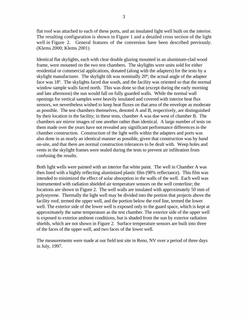
flat roof was attached to each of these ports, and an insulated light well built on the interior.The resulting configuration is shown in Figure 1 and a detailed cross section of the lightwell in Figure 2. General features of the conversion have been described previously.(Klems 2000; Klems 2001)

Identical flat skylights, each with clear double glazing mounted in an aluminum-clad woodframe, were mounted on the two test chambers. The skylights were units sold for eitherresidential or commercial applications, donated (along with the adapters) for the tests by askylight manufacturer. The skylight tilt was nominally 20º; the actual angle of the adapterface was 18º. The skylights faced due south, and the facility was oriented so that the normalwindow sample walls faced north. This was done so that (except during the early morningand late afternoon) the sun would fall on fully guarded walls. While the normal wallopenings for vertical samples were heavily insulated and covered with interior heat fluxsensors, we nevertheless wished to keep heat fluxes on that area of the envelope as moderateas possible. The test chambers themselves, denoted A and B, respectively, are distinguishedby their location in the facility; in these tests, chamber A was due west of chamber B. Thechambers are mirror images of one another rather than identical. A large number of tests onthem made over the years have not revealed any significant performance differences in thechamber construction. Construction of the light wells within the adapters and ports wasalso done in as nearly an identical manner as possible, given that construction was by handon-site, and that there are normal construction tolerances to be dealt with. Weep holes andvents in the skylight frames were sealed during the tests to prevent air infiltration fromconfusing the results.

Both light wells were painted with an interior flat white paint. The well in Chamber A wasthen lined with a highly reflecting aluminized plastic film (98% reflectance). This film wasintended to minimized the effect of solar absorption in the walls of the well. Each well wasinstrumented with radiation shielded air temperature sensors on the well centerline; thelocations are shown in Figure 2. The well walls are insulated with approximately 50 mm ofpolystyrene. Thermally the light well may be divided into the portion that projects above thefacility roof, termed the upper well, and the portion below the roof line, termed the lowerwell. The exterior side of the lower well is exposed only to the guard space, which is kept atapproximately the same temperature as the test chamber. The exterior side of the upper wellis exposed to exterior ambient conditions, but is shaded from the sun by exterior radiationshields, which are not shown in Figure 2. Surface temperature sensors are built into threeof the faces of the upper well, and two faces of the lower well.

The measurements were made at our field test site in Reno, NV over a period of three daysin July, 1997.

4

RESULTS

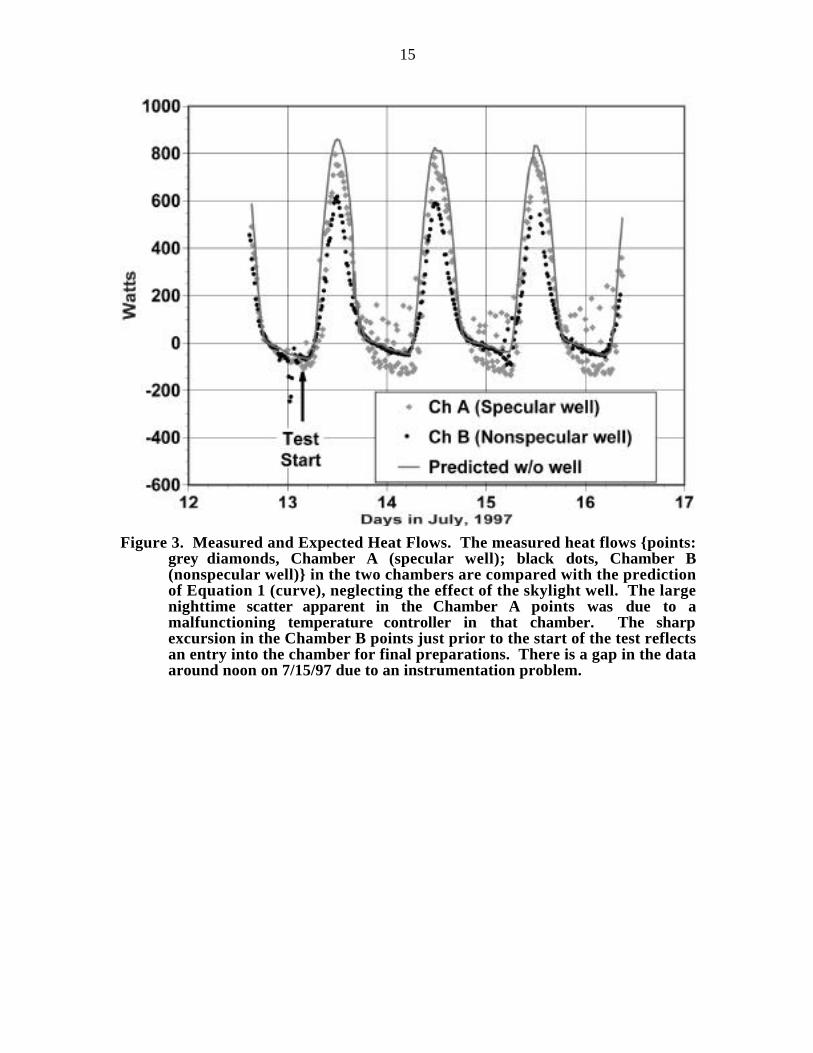
The measured skylight heat flow is shown for the three days of the tests in Figure 3. Thefacility records a variety of physical conditions as a function of time, and from these the netenergy flowing into the calorimeter can be derived from a dynamic net heat balance each 10minutes. Figure 3 plots each of these measurements as a point for each of the twochambers (gray diamonds, Chamber A; solid black circles, Chamber B). Each of theseseries of points then traces the measured heat flow as a function of time. Also plotted (as acontinuous curve) is the expected heat flow from Equation 1. Energy flows are defined aspositive flowing into the chamber; a negative heat flow represents a heat loss. In thiscalculation the interior temperature TI is taken to be the chamber (room) mean airtemperature, as would be done in a building energy simulation calculation. Since thiscalculation neglects the effect of the skylight well, and since the two chambers differ only inthe reflectivity and emissivity of the skylight well surfaces, the same curve would becalculated for either chamber.

The fact that the heat flows in the two chambers differ from each other and from theexpected curve demonstrates that the actual heat flow experienced by the architectural spacedepends on the effect of the skylight well. This effect can be substantial; as can be seen thepeak heat gain for the white-painted, nonspecular well (Chamber B) is around 25% lowerthan the expected curve. We note that this is a more architecturally realistic situation thanthe specular well of Chamber A, which was devised to minimize the well effect forsubsequent testing.

Unfortunately, for these tests the instrumentation in Chamber A was not functioning ideally.A temperature controller malfunction caused a small oscillation in the chamber airtemperature. This in turn appears as an oscillatory heat flow that is superimposed on thedata. Although the temperature excursions are generally less than half a degree Celsius, theresulting oscillatory heat flow error has a peak magnitude of up to 120 W. This isresponsible for the apparent large scatter of the points for Chamber A at night. Althoughless apparent, the malfunction continues during the daytime and is responsible for theapparent asymmetry of the daytime peaks. As a result, the data appears “noisy”; onecannot interpret short-term deviations from an expected curve as evidence against themodel. Long-term deviations, however, would be significant. (See the discussion of Figure6(a) below.) This problem did not affect Chamber B; while there are some small transientdepartures of the average air temperature in Chamber B from the set point (25 ºC) duringthe day, the resulting heat flow measurement errors are small and are not visible in thegraph.

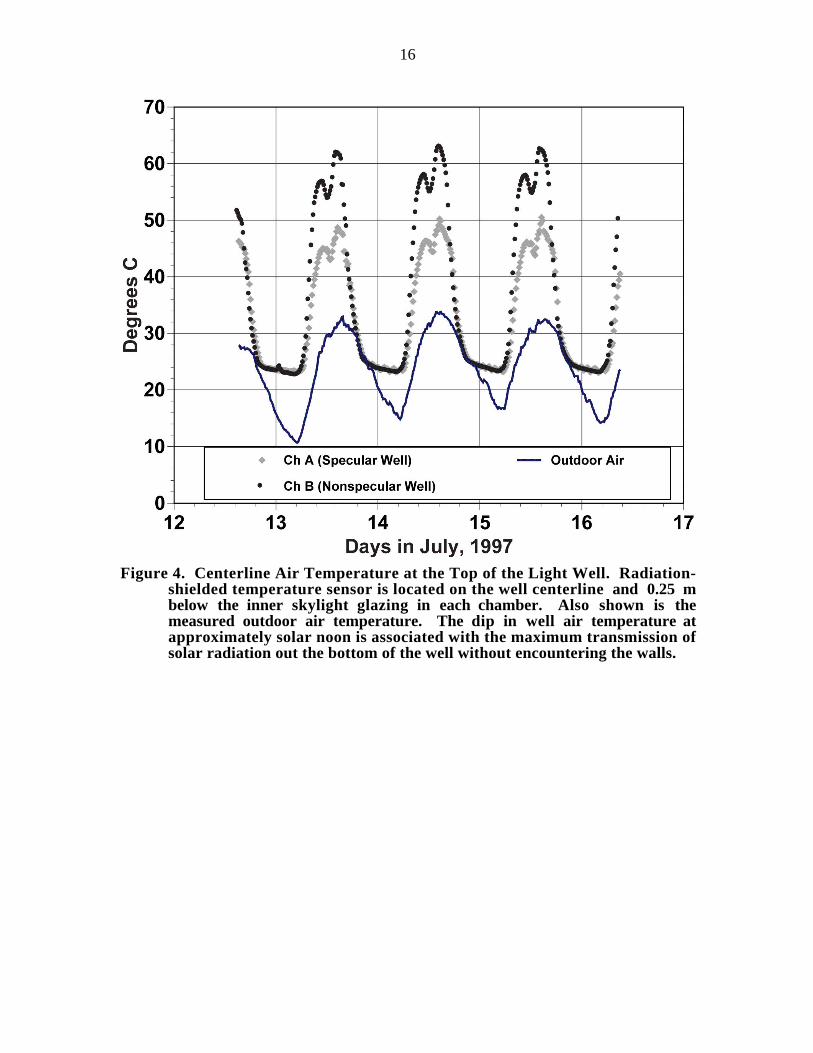
Figure 4 shows the measured air temperature near the top of the light well. This wasmeasured with a radiation-shielded thermistor located on the centerline of the light well 0.25m below the skylight, the uppermost of the temperature sensors shown in Figure 2. Alsoshown is the measured outdoor air temperature. During the day the air at the top of the wellis substantially hotter than both the outdoor air, and the chamber air temperature. Whileboth wells follow the same general pattern, the temperature in the nonspecular well is

5

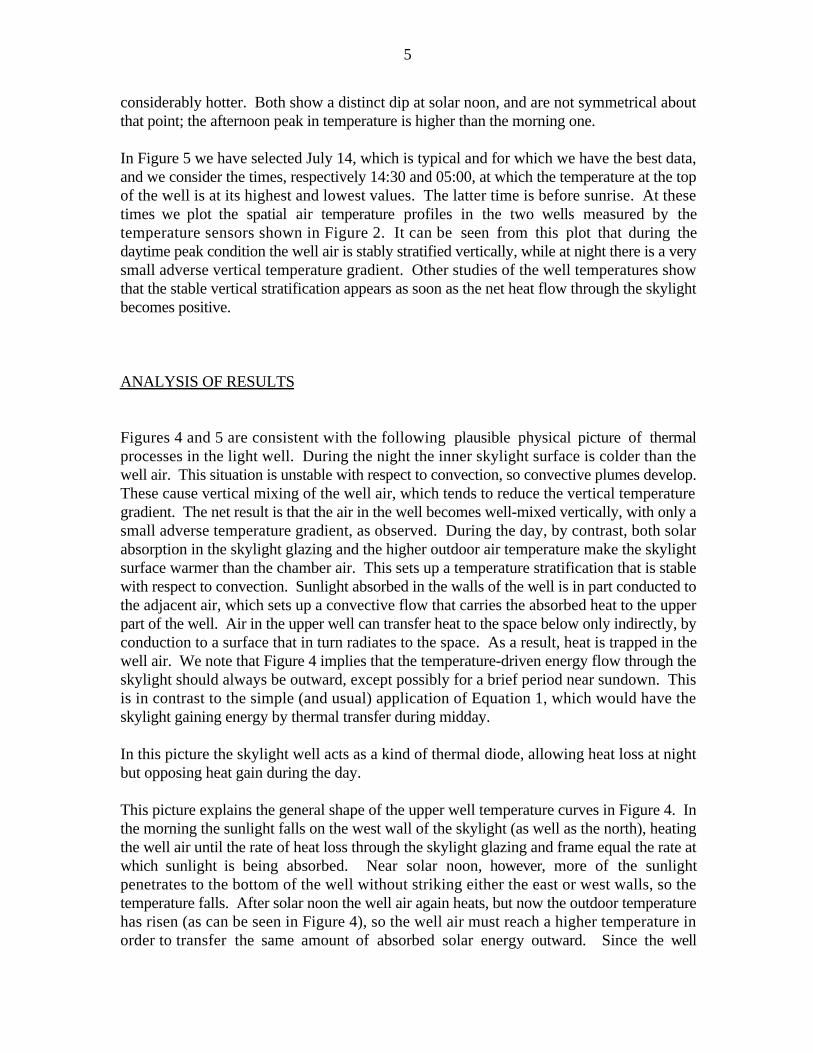
considerably hotter. Both show a distinct dip at solar noon, and are not symmetrical aboutthat point; the afternoon peak in temperature is higher than the morning one.

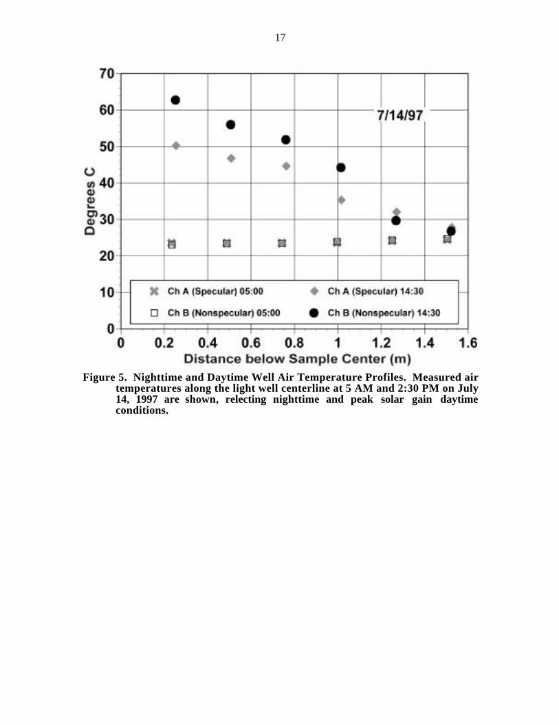
In Figure 5 we have selected July 14, which is typical and for which we have the best data,and we consider the times, respectively 14:30 and 05:00, at which the temperature at the topof the well is at its highest and lowest values. The latter time is before sunrise. At thesetimes we plot the spatial air temperature profiles in the two wells measured by thetemperature sensors shown in Figure 2. It can be seen from this plot that during thedaytime peak condition the well air is stably stratified vertically, while at night there is a verysmall adverse vertical temperature gradient. Other studies of the well temperatures showthat the stable vertical stratification appears as soon as the net heat flow through the skylightbecomes positive.

ANALYSIS OF RESULTS

Figures 4 and 5 are consistent with the following plausible physical picture of thermalprocesses in the light well. During the night the inner skylight surface is colder than thewell air. This situation is unstable with respect to convection, so convective plumes develop.These cause vertical mixing of the well air, which tends to reduce the vertical temperaturegradient. The net result is that the air in the well becomes well-mixed vertically, with only asmall adverse temperature gradient, as observed. During the day, by contrast, both solarabsorption in the skylight glazing and the higher outdoor air temperature make the skylightsurface warmer than the chamber air. This sets up a temperature stratification that is stablewith respect to convection. Sunlight absorbed in the walls of the well is in part conducted tothe adjacent air, which sets up a convective flow that carries the absorbed heat to the upperpart of the well. Air in the upper well can transfer heat to the space below only indirectly, byconduction to a surface that in turn radiates to the space. As a result, heat is trapped in thewell air. We note that Figure 4 implies that the temperature-driven energy flow through theskylight should always be outward, except possibly for a brief period near sundown. Thisis in contrast to the simple (and usual) application of Equation 1, which would have theskylight gaining energy by thermal transfer during midday.

In this picture the skylight well acts as a kind of thermal diode, allowing heat loss at nightbut opposing heat gain during the day.

This picture explains the general shape of the upper well temperature curves in Figure 4. Inthe morning the sunlight falls on the west wall of the skylight (as well as the north), heatingthe well air until the rate of heat loss through the skylight glazing and frame equal the rate atwhich sunlight is being absorbed. Near solar noon, however, more of the sunlightpenetrates to the bottom of the well without striking either the east or west walls, so thetemperature falls. After solar noon the well air again heats, but now the outdoor temperaturehas risen (as can be seen in Figure 4), so the well air must reach a higher temperature inorder to transfer the same amount of absorbed solar energy outward. Since the well

6

reflectance is much higher in the specular well the amount of absorbed solar energy islower, hence the well air temperature is lower overall.

Well Heat Flow

In order to make this physical picture quantitative, an additional effect must be considered.As indicated in Figure 2, the energy flow measured in this experiment, WMeas, is actually theheat flowing across the thermal aperture of the calorimeter chamber, which is effectively thebottom of the well. This differs from W , the energy flow through the skylight and frame, bythe heat flow S, through the walls of the skylight well. WMeas and W include, of course, bothheat and solar radiation. Since energy flows are defined as positive flowing into thechamber (or skylight well), the energy flow plotted in Figure 3 for the two chambers isreally

WMeas W S (2)

Although the light well was highly insulated during these experiments, S is by no meansnegligible. As can be seen from Figure 2, the exterior of the upper well is in contact withthe exterior air and that of the lower well with the air of the calorimeter guard space. Thelatter is kept at approximately the same temperature as the calorimeter air. We see fromFigure 4 that during the day S should be negative, while at night it should be positive for theupper well and very small for the lower.

The well heat flow was calculated as a weighted sum of the heat flow through the individualsurfaces of the upper and lower wells:

S qk AW(k )

k

(3)

where the index k runs over the eight faces of the skylight well (4 upper well, 4 lower well),qk and AW

(k ) are, respectively, the heat flow through and area of the kth surface, and of course

the total well surface area is AW AW( k )

k

. The individual surface heat fluxes were

calculated from a response factor series, (Mitalas 1968; Kusuda 1969)

qk( t) Yn(k ) TI

(k )( t n δ) TB Zn(k) TO

(k )( t n δ) TBn

, (4)

where TI( k ) and TO

( k ) are the time-dependent interior and exterior surface temperatures, TB isa constant base temperature (25º C) that cancels out of the calculation, δ is the time stepsize of the calculation (here, 10 minutes) and the response factors Yn

(k ) and Zn(k ) were

calculated from the properties of the construction. The program WALFERF (Davis andBull unpub.), which is based on a published calculation (Myers 1980), was used to calculatethe response factors. This program had previously been checked against both DOE2

7

(Building Energy Simulation Group and Solar Energy Group 1993; Winkelmann, Birdsallet al. 1993) and HEATING7 (Childs 1991).

In a subsequent test (Klems 2001) heat flow sensors were installed in two sections of theskylight well wall and the calculation of Equation 4 compared with the measured heatfluxes. On the basis of those tests, we estimate that the level of error in the calculation of Shere is 21 W for Chamber A, and 38 W for Chamber B. Since in all the tests S is small atnight, the principle contribution to these errors (which are RMS averages over time) is fromdaytime heat flows.

A Simple Skylight Model

The simplest method of including the skylight well effect is to use Equation 1 to model theskylight heat flow, W , in Equation 2, but to use the local air temperature for the temperatureTI in that equation, rather than the space air temperature. For each data point, weextrapolated the measured air temperature from the highest measured location, 0.25 m belowthe skylight surface to the height of the skylight center, using the highest and next highesttemperature sensors to estimate the local vertical temperature gradient. The U-factor used inthis calculation was calculated with WINDOW4 (Finlayson, Arasteh et al. 1993; Arasteh,Finlayson et al. 1994) and THERM, (Finlayson, Mitchell et al. 1998) using NFRC standardsummer conditions.(NFRC 1991) This U-factor, which was also used in the calculation ofcurve 1 and in Figure 3, did include some effects of the well in that the THERM calculationtook into account the effects of longwave radiant exchange in the well enclosure. (We havetermed this a calculation "neglecting the well" because it is the sort of calculation that mightbe done based on an architectural plan that ignores the well geometry. It uses onlytemperatures outside the well to define its boundary conditions, and once the wellcharacteristics have been used limitedly in the calculation of the U-factor (in a mannersimilar to the way 2D frame calculations are included), the skylight is then treated as apurely planar object.) The direct normal solar intensity EDN and the total incident flux onthe skylight were measured directly; from these measurements the quantity (Ed Er ) wascalculated. The correct value of the solar incident angle and SHGC(θ) were calculated at

each data point from the time and solar position.

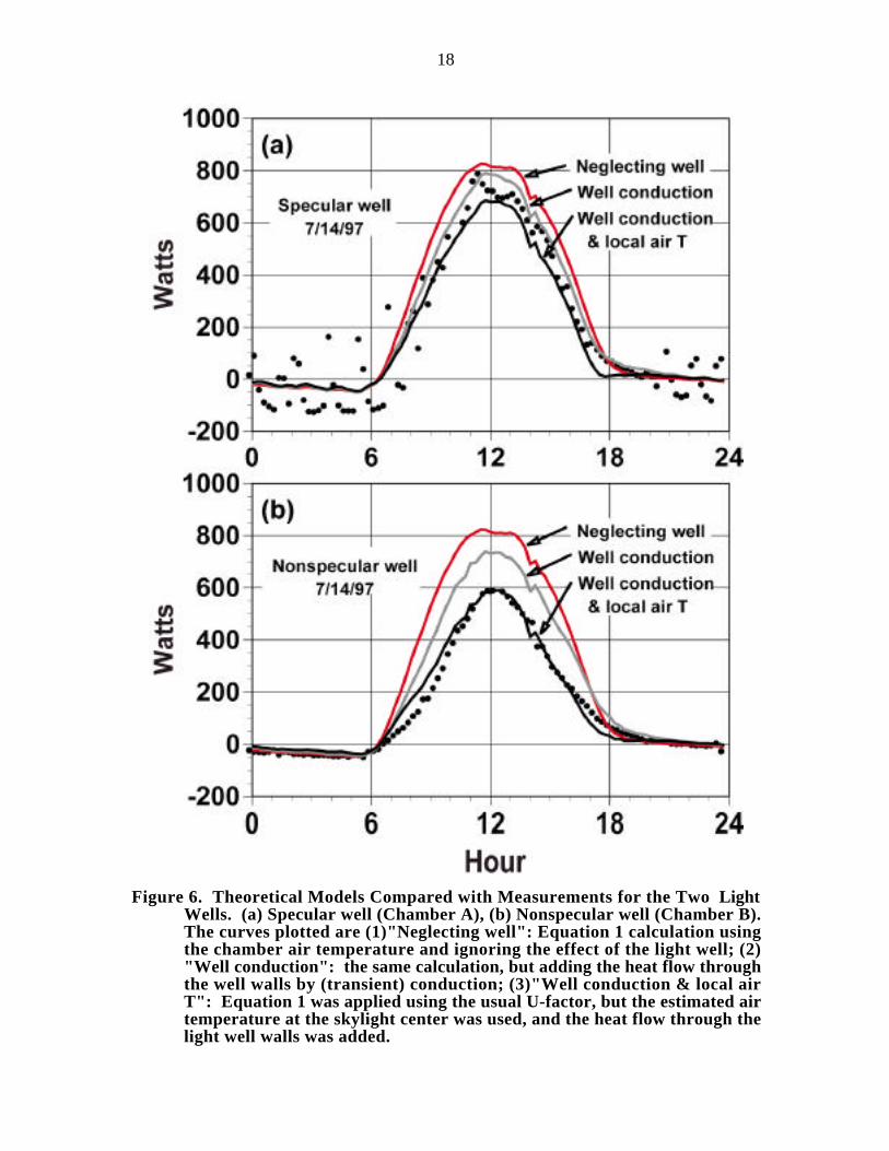
Figure 6 compares this model to the measured data and shows the effect of the correctionfor well heat flow. Data is shown as an hourly plot for July 14, 1997, which is both typicalof the data and is the day for which the data are of the best quality. Results are comparedseparately for each chamber. Three curves are shown. Curve 1 is a repeat of the originalcalculation of Equation 1 neglecting the skylight well shown in Figure 3; it represents ourstarting point. Next, in curve 2, is shown the effect of including Equation 2 in thiscalculation; this shows the effect of the skylight well heat transfer. Finally, in curve 3 thesimple model described above is used to calculate W in Equation 2.

The model matches the data very well for the nonspecular well, as can be seen from Figure6(b). Those regions of the curve that systematically differ from the data are still within the38W uncertainty range of the well heat flow calculation. For the specular well (Figure 6(a))the model is also in agreement with the data, although this is less easy to see in the figure

8

because of the spurious effects of the air temperature oscillation. In the nonspecular wellcurve 2 shows that heat flow through the well walls accounts for around one-third of thediscrepancy between the data and the original Equation 1 calculation neglecting the well.

Detailed Model

We also constructed a detailed U-factor model intended to match the experimentalconditions more closely than does the NFRC calculation. We conceptualized the(temperature-driven) heat flow through the skylight as the area-weighted sum of a one-dimensional glazing heat flux and a one-dimensional frame heat flux. The weighting areaswere the vision area and the physical interior surface area of the frame, respectively. Each ofthese one-dimensional heat fluxes was taken to consist of an exterior heat flux dependingon exterior conditions and the exterior surface temperature, a "conductance"' heat flux,depending on the interior and exterior surface temperatures of the glazing or frame, and aninterior heat flux depending on interior conditions and the interior surface temperature.

The exterior heat flux was calculated from the measured sky temperature, air temperatureand wind speed, in addition to the exterior surface temperature. The WINDOW4 equationfor convective coefficient as a function of wind speed for a tilted surface was used. For theframe the "conductance" heat flux was calculated using a frame conductance derived fromthe WINDOW4/THERM U-factor calculation in the simple model. Effectively thisconductance includes the correction for 2D conduction at the edge of the glazing. For theglazing the WINDOW4 equations for convective and radiative heat transfer across an airgap were used; the small temperature drop in the glass layers was neglected. The interiorheat flux was modeled as (1) a convective part, using the WINDOW4 convective coefficientrelation and the local air temperature (extrapolated to the height of the center of the glazing),and (2) a detailed model of radiation between the glazing or frame and the light well. In thismodel, the light well was divided into 4 parts vertically, and the north, south, east, and westfaces were treated separately, resulting in a total of 16 sections. For each section the viewfactor to the window or frame was calculated, and the net radiative heat transfer wascalculated from the interior glazing or frame surface temperature and the well sectionsurface temperature. A given well section was assumed to have a surface temperature equalto the well air temperature interpolated to the height of the center of the well section. (Thisassumption should slightly overestimate the radiant heat transfer.) The bottom of the wellwas modeled as a black surface at the mean chamber temperature. (All of the other wellsurfaces were assumed to have an emissivity of 0.9 for the non-specular well, an 0.03 forthe specular well.)

The assumed interior and exterior surface temperatures were iterated to obtain agreementbetween the calculated exterior, interior, and "conductance" fluxes. Since there is radianttransfer between the inner surface of the glazing and that of the frame, iteration of the twoheat fluxes was coupled. The nth iteration of the frame and glazing heat fluxes used the(n 1) st values of the interior and exterior surface temperatures for the frame and glazing.Five iterations were carried out for each data point, and this sufficed to produce agreementof the interior, exterior and "conductance" heat fluxes to better than 0.01W/m2 (generallymuch less).

9

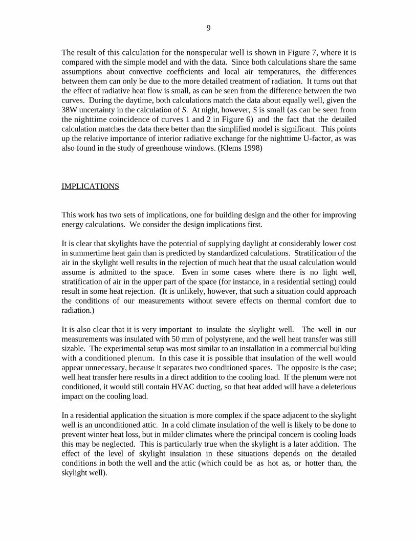
The result of this calculation for the nonspecular well is shown in Figure 7, where it iscompared with the simple model and with the data. Since both calculations share the sameassumptions about convective coefficients and local air temperatures, the differencesbetween them can only be due to the more detailed treatment of radiation. It turns out thatthe effect of radiative heat flow is small, as can be seen from the difference between the twocurves. During the daytime, both calculations match the data about equally well, given the38W uncertainty in the calculation of S. At night, however, S is small (as can be seen fromthe nighttime coincidence of curves 1 and 2 in Figure 6) and the fact that the detailedcalculation matches the data there better than the simplified model is significant. This pointsup the relative importance of interior radiative exchange for the nighttime U-factor, as wasalso found in the study of greenhouse windows. (Klems 1998)

IMPLICATIONS

This work has two sets of implications, one for building design and the other for improvingenergy calculations. We consider the design implications first.

It is clear that skylights have the potential of supplying daylight at considerably lower costin summertime heat gain than is predicted by standardized calculations. Stratification of theair in the skylight well results in the rejection of much heat that the usual calculation wouldassume is admitted to the space. Even in some cases where there is no light well,stratification of air in the upper part of the space (for instance, in a residential setting) couldresult in some heat rejection. (It is unlikely, however, that such a situation could approachthe conditions of our measurements without severe effects on thermal comfort due toradiation.)

It is also clear that it is very important to insulate the skylight well. The well in ourmeasurements was insulated with 50 mm of polystyrene, and the well heat transfer was stillsizable. The experimental setup was most similar to an installation in a commercial buildingwith a conditioned plenum. In this case it is possible that insulation of the well wouldappear unnecessary, because it separates two conditioned spaces. The opposite is the case;well heat transfer here results in a direct addition to the cooling load. If the plenum were notconditioned, it would still contain HVAC ducting, so that heat added will have a deleteriousimpact on the cooling load.

In a residential application the situation is more complex if the space adjacent to the skylightwell is an unconditioned attic. In a cold climate insulation of the well is likely to be done toprevent winter heat loss, but in milder climates where the principal concern is cooling loadsthis may be neglected. This is particularly true when the skylight is a later addition. Theeffect of the level of skylight insulation in these situations depends on the detailedconditions in both the well and the attic (which could be as hot as, or hotter than, theskylight well).

10

Consciously utilizing the heat trapping properties of a skylight well could yield systemswith still better rejection of solar heat for a given amount of daylight than the skylights inthis test. For example, venting the skylight during the daytime in summer could yield betterheat rejection than found here. Based on our results it seems likely that systems such astubular skylights, which have proportionately very long wells, together with specialprovisions for efficient light transfer down these wells, have the potential for providingdaylight with very low solar heat load. The daylight transmission system would need toinclude provisions for rejecting solar infrared, such as selectively reflective coatings. It isalso clear that in such systems special attention must be paid to durability issues raised bythe temperatures that the upper parts of the systems will experience.

The implications for improving energy calculations are, first, that little new work is needed atthe components level. The present tools are adequate for predicting the behavior ofskylights, and only a relatively simple model is necessary, provided that the local airtemperature is known. This, however, is a difficulty. Present building energy simulationprograms use single air node models and cannot predict temperature stratification. Evenmodeling the light well as a separate space would not produce a very accurate calculation ofthe skylight heat transfer, because, as can be seen from Figure 5, the air temperature at theskylight is not close to the average air temperature of the well. Further research should bedirected toward finding methods of predicting the air temperature near the skylight, and theinterior convection surface heat transfer coefficients. It is likely that properly validatedcomputational fluid dynamics (CFD) calculations will be necessary to form a basis for thesepredictions, since convection is the principal determinant of the temperature distributionwithin the well.

ACKNOWLEGMENT

This work was supported by the Assistant Secretary for Energy Efficiency and RenewableEnergy, Office of Building Technology, State and Community Programs, Office ofBuilding Research and Standards of the U.S. Department of Energy under Contract No.DE-AC03-76SF00098.

The assistance of Velux-America, which provided the skylights and well adapters used inthis project, is gratefully acknowledged, and special thanks are due to Roland Temple for hisenthusiastic assistance in planning and preparation.

The author is grateful to the members of the MoWiTT technical staff, DennisDiBartolomeo, Guy Kelley, Michael Streczyn and Mehrangiz Yazdanian, whose diligence inrunning and maintaining the MoWiTT were vital to the success of this project.

We are indebted to the Experimental Farm, University of Nevada at Reno, for theirhospitality in providing a field site and for their cooperation in our activities.

11

REFERENCES

Arasteh, D. K., E. U. Finlayson and C. Huizenga (1994). WINDOW 4.1: A PC Programfor Analyzing the Thermal Performance of Fenestration Products. LawrenceBerkeley National Laboratory, LBL-35298.

Building Energy Simulation Group, L. B. L. and L. A. N. L. Solar Energy Group (1993).DOE-2 Engineers Manual, Version 2.1A. Lawrence Berkeley Laboratory, LBL-11353.

Childs, K. W. (1991). HEATING 7.1 User's Manual. Oak Ridge, TN, Oak Ridge NationalLaboratory.

Davis, P. K. and J. C. Bull (unpub.). WALFERF.

Finlayson, E., R. Mitchell, D. Arasteh, C. Huizenga and D. Curcija (1998). THERM 2.0:Program Description: A PC Program for Analyzing the Two-Dimensional HeatTransfer Through Building Products. Lawrence Berkeley National Laboratory,LBL-37371 Rev. 2.

Finlayson, E. U., D. K. Arasteh, C. Huizenga, M. D. Rubin and M. S. Reilly (1993).WINDOW 4.0: Documentation of Calculation Procedures. Lawrence BerkeleyLaboratory, Berkeley, CA 94720, Technical Report LBL-33943.

Klems, J. H. (1992). “Method of Measuring Nighttime U-Values Using the MobileWindow Thermal Test (MoWiTT) Facility.” ASHRAE Trans. 98(Pt. II): 619-29.

Klems, J. H. (1998). “Greenhouse Window U-Factors Under Field Conditions.”ASHRAE Trans. 104(Pt. 1): Paper no. SF-98-3-1.

Klems, J. H. (2000). “U-Values of Flat and Domed Skylights.” ASHRAE Trans. 106(2):Symposium MN-00-7-3.

Klems, J. H. (2001). “Net Energy Measurements on Electrochromic Skylights.” Energyand Buildings 33: 93-102.

Klems, J. H., S. Selkowitz and S. Horowitz (1982). A Mobile Facility for Measuring NetEnergy Performance of Windows and Skylights. Proceedings of the CIB W67Third International Symposium on Energy Conservation in the Built Environment.Dublin, Ireland, An Foras Forbartha. III: 3.1.

Kusuda, T. (1969). “Thermal Response Factors for Multi-Layer Structures of VariousHeat Conduction Systems.” ASHRAE Trans. 75(pt. 1): 246-271.

12

Mitalas, G. P. (1968). “Calculation of Transient Heat Flow Through Walls and Roofs.”ASHRAE Trans. 74(Pt. 2): 181.

Myers, G. E. (1980). “Long-Time Solutions to Heat-Conduction Transients with Time-Dependent Inputs.” J. Heat Trans. 102: 115-120.

NFRC (1991). NFRC 100-91: Procedure for Determining Fenestration Product ThermalProperties (Currently Limited to U-Value). National Fenestration Rating Council,Silver Sping, MD 20910.

Winkelmann, F. C., B. E. Birdsall, W. F. Buhl, K. L. Ellington, A. E. Erkem, J. J. Hirschand S. Gates (1993). DOE-2 Supplement, Version 2.1E. Lawrence BerkeleyNational Laboratory, LBL-34947.

13

FIGURES

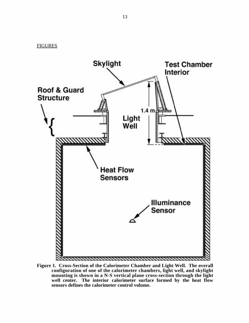
Figure 1. Cross-Section of the Calorimeter Chamber and Light Well. The overallconfiguration of one of the calorimeter chambers, light well, and skylightmounting is shown in a N-S vertical plane cross-section through the lightwell center. The interior calorimeter surface formed by the heat flowsensors defines the calorimeter control volume.

14

Figure 2. Detail of the Light Well and Skylight. The apertures defining the"vision" area and the skylight thermal area (heavy dashed arrow) areshown, as is the chamber effective thermal aperture (heavy dashed arrow).The heat flow WMeas crossing this aperture and the heat flow, S, through thewell sides are illustrated schematically, along with the skylight heat flow,W. Also shown are the locations of the well centerline air temperaturesensors.

15

Figure 3. Measured and Expected Heat Flows. The measured heat flows {points:grey diamonds, Chamber A (specular well); black dots, Chamber B(nonspecular well)} in the two chambers are compared with the predictionof Equation 1 (curve), neglecting the effect of the skylight well. The largenighttime scatter apparent in the Chamber A points was due to amalfunctioning temperature controller in that chamber. The sharpexcursion in the Chamber B points just prior to the start of the test reflectsan entry into the chamber for final preparations. There is a gap in the dataaround noon on 7/15/97 due to an instrumentation problem.

16

Figure 4. Centerline Air Temperature at the Top of the Light Well. Radiation-shielded temperature sensor is located on the well centerline and 0.25 mbelow the inner skylight glazing in each chamber. Also shown is themeasured outdoor air temperature. The dip in well air temperature atapproximately solar noon is associated with the maximum transmission ofsolar radiation out the bottom of the well without encountering the walls.

17

Figure 5. Nighttime and Daytime Well Air Temperature Profiles. Measured airtemperatures along the light well centerline at 5 AM and 2:30 PM on July14, 1997 are shown, relecting nighttime and peak solar gain daytimeconditions.

18

Figure 6. Theoretical Models Compared with Measurements for the Two LightWells. (a) Specular well (Chamber A), (b) Nonspecular well (Chamber B).The curves plotted are (1)"Neglecting well": Equation 1 calculation usingthe chamber air temperature and ignoring the effect of the light well; (2)"Well conduction": the same calculation, but adding the heat flow throughthe well walls by (transient) conduction; (3)"Well conduction & local airT": Equation 1 was applied using the usual U-factor, but the estimated airtemperature at the skylight center was used, and the heat flow through thelight well walls was added.

19

Figure 7. Two Theoretical Models Compared with Measurements, NonspecularWell. Grey curve: assuming constant (NFRC) U-factor. Black curve:detailed theoretical model of heat flux described in the text. Both curveshave the effect of heat conduction through the well walls included.

20

Appendix A. Nomenclature

Symbols

AV Area (projected into the glazing plane) of the transparent ("vision")portion of a fenestration.

AT Total ("rough opening") projected area of a fenestration system,including frame.

AW Total inside area of the skylight well.

AW(k ) Area of the kth skylight well surface.

EDN Direct normal solar irradiance.

Ed Diffuse solar irradiance incident on the fenestration.

Er Ground-reflected solar irradiance incident on the fenestration.

θ Solar incident angle.

qk Heat flux through the kth skylight well surface.

SHGC (θ) Solar Heat Gain Coefficient for incident beam radiation at an incidence

angle θ.

SHGC D Solar Heat Gain Coefficient for diffuse incident radiation.

TI Interior temperature.

TO Exterior temperature.

TI( k ) Interior temperature for the kth well surface.

TO( k ) Exterior temperature for the kth well surface.

∆T Difference TO - TI.

U Thermal transmittance ("U-factor").

W Energy flow through the fenestration (here: skylight), defined positivefor flow into the space.

Yn(k ) Same-side response factor for the kth well surface.

Zn(k ) Cross-element response factor for the kth well surface.