Solar múltiple optimization for a solar-only thermal power plant, using oil as heat transfer fluid in the parabolic trough collectors

M.J. Montes , A. Abánades , J.M. Martínez-Val , M. Valdés

E.T.S. I Industriales - U.N.E.D., CIJuan del Rosal, 12, 28040 Madrid, Spain E.T.S.I.Industriales - U.P.M., C/José Gutiérrez Abascal, 2, 28006 Madrid, Spain

Abstract

Usual size of parabolic trough solar thermal plants being built at present is approximately 50 MWe. Most of these plants do not have a thermal storage system for maintaining the power block performance at nominal conditions during long non-insolation periods. Because of that, a proper solar field size, with respect to the electric nominal power, is a fundamental choice. A too large field will be partially useless under high solar irradiance valúes whereas a small field will mainly make the power block to work at part-load conditions.

This paper presents an economic optimization of the solar múltiple for a solar-only parabolic trough plant, using neither hybridiza-tion ñor thermal storage. Five parabolic trough plants have been considered, with the same parameters in the power block but different solar field sizes. Thermal performance for each solar power plant has been featured, both at nominal and part-load conditions. This char-acterization has been applied to perform a simulation in order to calcúlate the annual electricity produced by each of these plants. Once annual electric energy generation is known, levelized cost of energy (LCOE) for each plant is calculated, yielding a minimum LCOE valué for a certain solar múltiple valué within the range considered.

Keywords: Solar-only thermal power plant; Parabolic trough collector; Solar múltiple; Optimization

1. Introduction

Parabolic trough technology has proven to be the most mature and lowest cost solar thermal technology available today (Price et al., 2002). As a result, most of the projects for the construction of commercial solar thermal power plants are based on this type of collectors; several parabolic trough power plants are going to be constructed in USA, Spain, Northern África, Middle East, etc. Most of these plants consist of a solar field, a steam generator, a power cycle and a fossil-fuel fired back-up system.

Thermal storage system is not commonly employed in current parabolic trough plants, although there are some exceptions, like Andasol-1, in Spain, with 7.7 equivalent-hours of indirect storage in two tanks of molten salts (Rel-loso and Gutiérrez, 2008). In the latter case, storage is nec-essary to minimize the effect of transients, since only a 2% of fossil hybridization is allowed in Nevada, so this energy supplement is mostly used in order to prevent oil freezing. It is expected that more future parabolic trough plants will have thermal storage systems, because the operation strat-egy adopted in this way can be a scheduled mode, instead of the current solar dispatching mode.

Fossil-fuel hybridization is usually performed by means of an auxiliary oil heater able to maintain oil temperature above a lower limit, and a fossil-fuel fired boiler, which

Nomenclature

^mO

kp

m mre{

Pi

Pi

Pl,reí

P2,reí

parameter defining the shape of the pump effi-ciency curve, -constant for pressure drop calculations, -mass flow rate, kg/s reference mass flow rate, kg/s inlet pressure to the chosen section of the tur-bine, bar exhaust pressure from the chosen section of the turbine, bar reference inlet pressure to the chosen section of the turbine, bar reference exhaust pressure from the chosen sec­tion of the turbine, bar

6th,soiar_fieid thermal power produced in the solar field,

Sth.PB

SM¿esi

VA

W thermal power demanded by the power block, W

»njoint solar múltiple at design-point conditions, -overall heat transfer coefficient, W/°C

UAreí reference overall heat transfer coefficient, W/°C AP pressure drop, bar >/generator generator efficiency, ->/s,pump isentropic pump efficiency, -*?s, pump o isentropic pump efficiency at nominal condi­

tions, -vs, turbine

isentropic turbine efficiency, -*?s, turbine o isentropic turbine efficiency at nominal con­

ditions, -9 incident angle, degrees K(6) incident angle modifier, -

Acronyms DCA drain cooling approach ET-150 Eurotrough-150 HTF heat transfer fluid LCOE levelized cost of energy TTD terminal temperature difference

produces steam to turbine seáis, in order to keep the turbine heated. Both systems opérate during night and long non-insolation periods. Because of máximum fuel consumption is usually limited by the national electricity feed-in law, the remainder of annual fossil-fuel percentage for electricity pro-duction is very low if the solar plant is going to apply for incentives. For this reason no electricity production from fossil fuel has been considered in this paper.

The heat transfer fluid in the solar field is usually oil, so a steam generator is needed between the solar field and the Rankine steam turbine cycle. This particular configuration is called heat transfer fluid (HTF) technology.

The operation strategy adopted for the solar-only para-bolic trough plant considered, is the solar dispatching mode, and the nominal electrical power has been set to 50 MWe net, because it is an usual size for current para-bolic trough plants. An optimization of the solar field size has been carried out for this particular configuration. As the solar field represents the major plant investment, calcu­laron of the optimum field size is an analysis described in other works (Quaschning et al., 2002). The optimization presented in this paper involves the calculation of the solar múltiple for which the levelized cost of energy is minimum. Solar múltiple is defined as the ratio between the thermal power produced by the solar field at the design point and the thermal power required by the power block at nominal conditions:

SM design _point 0 th .solar _field

0 th ,power-block (i)

This parameter represents the solar field size related to the power block, in terms of nominal thermal power. Design-point conditions adopted for this particular analy­sis will be summarized in Section 2.2.1. Solar múltiple for solar-only plants is always greater that one, in order to achieve nominal conditions on the power block during a time interval longer than the one obtained if solar múltiple is equal to one, as it can be seen in Fig. 1. Nevertheless, large solar múltiple valúes for parabolic trough plants without thermal storage lead to a thermal energy overpro-duction that cannot be used for electricity generation. Although this configuration enables the power block to work at nominal conditions during longer periods of time, the cost of the kWhe will be higher because there is a given non-profitable solar field inversión.

Nominal performance interval

Nominal performance point

Energy lost (Solar-only plant)

Power Block Thermal Power Demand

Solar Field Thermal Power

forSM=1.5

design _point

Time(h)

Fig. 1. Daily thermal power production for different solar field múltiples.

As it will be seen in Section 2, the solar thermal plant configurations selected will have solar múltiple ranges from 1 to 1.5. The exact valué in each case will depend on the nominal thermal power produced in the solar field, because the nominal thermal power demanded by the steam gener-ator will be the same for all the plants considered, as the 50 MWe power cycle is the same for all the cases. Neverthe-less, in Section 4, it will be also exposed that optimum solar múltiple depends not only on the solar field size, but also on the plant location, the design point and the power cycle parameters at nominal conditions.

Nominal and part-load behaviour of every thermal sys-tem used in the simulation have been compared with real data and other models. The annual simulation program has been compared with other parabolic trough plants assessment programs (Lippke, 1995; Quaschning et al., 2002). One of the main features of this new model is that it has been developed on the basis of theoretical equations rather than empirical correlations: the collector model is based on heat transfer correlations in a cross-section and along its length; the equations to simúlate nominal and part-load Rankine cycle are the usually employed for these cycles. References on those equations and physical models will be given in detail in the corresponding section. Because of that, one has the possibility of changing configuration parameters of both the solar field and the power cycle, like collector optical or geometrical parameters or turbine configuration.

2. Solar thermal plant nominal performance at design-point conditions

2.1. Rankine steam cycle parameters at nominal conditions

The power block considered is a regenerative 50 MWe

Rankine cycle. According to the size of the cycle, it is advis-able to have six regenerative heat feeders, i.e., the feed water will be preheated in three low pressure closed feed-water heaters, a deaerator, and two high pressure closed feedwater heaters.

The type of heat transfer fluid in the solar field and its operating temperature range determine the steam turbine inlet conditions. Because of thermal stability of Therminol VP-1 is only kept up to working temperatures of 400 °C, the máximum steam temperature in the power cycle will be nearly 370 °C. In order to avoid a great humidity frac-tion in steam at the turbine exhaust, steam reheating is necessary.

Power cycle must perform at part-load conditions when not enough solar thermal power is available. Section 3 deals with part-load operation. In this section, only full load conditions are studied. Nominal valúes for the main parameters in the cycle are summarized in Table 1.

Extraction steam pressures are calculated at nominal conditions in such a way that enthalpy drops are identical along the expansión turbine line, in the Mollier diagram. It

Table 1

Nominal valúes for the 50 MWe steam power cycle.

Main parameters valué for the 50 MWe steam power cycle

Turbine Inlet temperature (°C) Inlet pressure (bar) High pressure turbine efficiency (%) Low pressure turbine efficiency (%) Electro-mechanical efficiency (%)

Extraction point pressures Extraction no. Extraction no. Extraction no. Extraction no. Extraction no. Extraction no.

1 (bar) 2 (bar) 3 (bar) 4 (bar) 5 (bar) 6 (bar)

Pressure drop in extraction and reheating line Extraction line no. Extraction line no. Reheating line (%) Extraction line no. Extraction line no. Extraction line no. Extraction line no.

1 (%) 2 (%)

3 (deaerator) (%) 4 (%) 5 (%) 6 (%)

Condenser pump Pl Isentropic efficiency Electro-mechanical efficiency

Feedwater pump P2 Isentropic efficiency Electro-mechanical efficiency

Lowlhigh pressure closed feedwater heaters Terminal temperature difference (°C) Drain cooling approach (°C)

Condenser Condensing pressure (bar)

Steam generator Thermal efficiency (%) Total pressure drop (water side) (bar)

370 90 85.5 89.5

45.4 20.6 8.75 3.627 1.224 0.3461

2.5 3 11.75 4.5 3 3 3.5

75

78 98

1.5 5.5

0.08

98 4.5

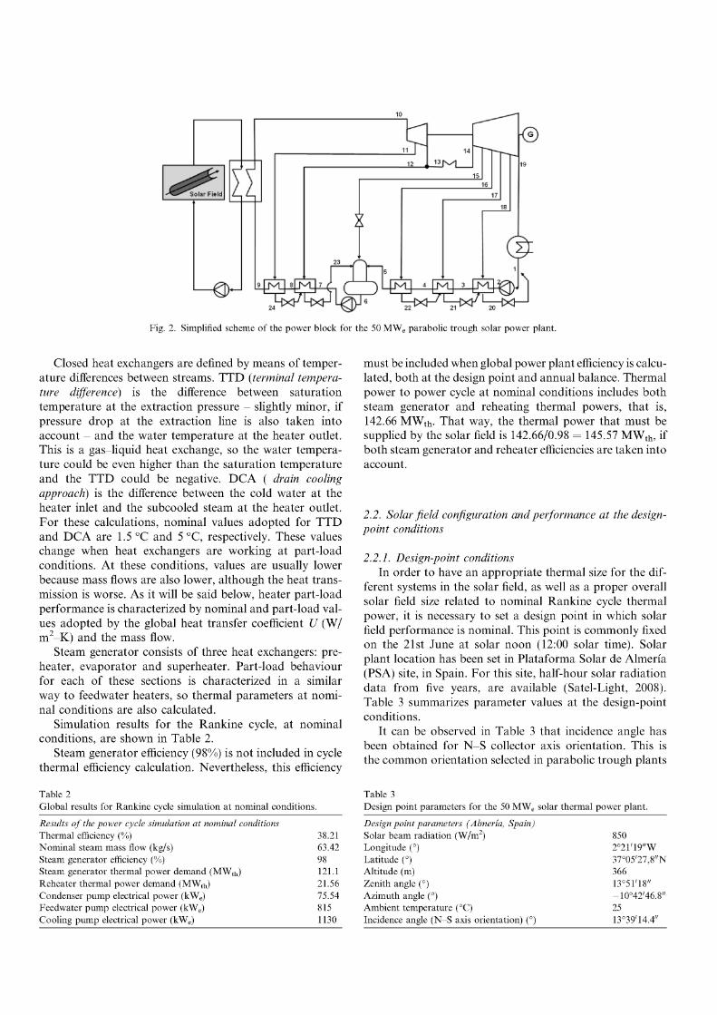
has been demonstrated that this arrangement lead to a high cycle efficiency (Kostyuk and Frolov, 1988). There are two extractions from the high pressure turbine and four extrac-tions from the low pressure turbine. The second extraction point matches up with the high pressure turbine outlet, as it is shown in Fig. 2. In the same figure it can be seen that reheating is performed between high and low pressure tur-bines, so low pressure turbine inlet temperature is set to 370 °C at nominal conditions. Pressure drop in extraction and reheating lines has been defined in percentage terms, related to turbine extraction pressures, as it can be seen in Table 1.

Condensing pressure valué (0.08 bar) is referred to a water cooled condenser. Water is pumped through the cooling system by a pump located at the cooling tower out­let. Owing to the great water mass flow necessary to cool the condenser (about 2800 kg/s at nominal conditions), electric power consumed by this pump must be considered as one of the main internal consumptions of the solar ther­mal power plant.

t¡Ss

L_^)J b^FMFTW ¿ p L £ ^ 21 • " " 20

Fig. 2. Simplified scheme of the power block for the 50 MWe parabolic trough solar power plant.

Closed heat exchangers are defined by means of temper­ature differences between streams. TTD (terminal tempera-ture difference) is the difference between saturation temperature at the extraction pressure - slightly minor, if pressure drop at the extraction line is also taken into account - and the water temperature at the heater outlet. This is a gas-liquid heat exchange, so the water tempera-ture could be even higher than the saturation temperature and the TTD could be negative. DCA ( drain cooling approach) is the difference between the cold water at the heater inlet and the subcooled steam at the heater outlet. For these calculations, nominal valúes adopted for TTD and DCA are 1.5 °C and 5 °C, respectively. These valúes change when heat exchangers are working at part-load conditions. At these conditions, valúes are usually lower because mass flows are also lower, although the heat trans-mission is worse. As it will be said below, heater part-load performance is characterized by nominal and part-load val­úes adopted by the global heat transfer coefficient U (W/ m2-K) and the mass flow.

Steam generator consists of three heat exchangers: pre-heater, evaporator and superheater. Part-load behaviour for each of these sections is characterized in a similar way to feedwater heaters, so thermal parameters at nomi­nal conditions are also calculated.

Simulation results for the Rankine cycle, at nominal conditions, are shown in Table 2.

Steam generator efficiency (98%) is not included in cycle thermal efficiency calculation. Nevertheless, this efficiency

must be included when global power plant efficiency is calcu­lated, both at the design point and annual balance. Thermal power to power cycle at nominal conditions includes both steam generator and reheating thermal powers, that is, 142.66 MWth- That way, the thermal power that must be supplied by the solar field is 142.66/0.98 = 145.57 MW th, if both steam generator and reheater efficiencies are taken into account.

2.2. Solar field configuration and performance at the design-point conditions

2.2.1. Design-point conditions In order to have an appropriate thermal size for the dif-

ferent systems in the solar field, as well as a proper overall solar field size related to nominal Rankine cycle thermal power, it is necessary to set a design point in which solar field performance is nominal. This point is commonly fixed on the 21st June at solar noon (12:00 solar time). Solar plant location has been set in Plataforma Solar de Almería (PSA) site, in Spain. For this site, half-hour solar radiation data from five years, are available (Satel-Light, 2008). Table 3 summarizes parameter valúes at the design-point conditions.

It can be observed in Table 3 that incidence angle has been obtained for N-S collector axis orientation. This is the common orientation selected in parabolic trough plants

Table 2 Global results for Rankine cycle simulation at nominal conditions.

Results of the power cycle simulation at nominal conditions Thermal efficiency (%) Nominal steam mass flow (kg/s) Steam generator efficiency (%) Steam generator thermal power demand (MWth) Reheater thermal power demand (MWj,) Condenser pump electrical power (kWe) Feedwater pump electrical power (kWe) Cooling pump electrical power (kWe)

Table 3 Design point parameters for the 50 MWe solar thermal power plant.

38.21 63.42 98 121.1 21.56 75.54 815 1130

Design point parameters (Almería, Solar beam radiation (W/m2) Longitude (°) Latitude (°) Altitude (m) Zenith angle (°) Azimuth angle (°) Ambient temperature (°C)

Spain)

Incidence angle (N-S axis orientation) (°)

850 2°21'19"W 37°05'27,8"N 366 13°51'18" -10°42'46.8" 25 13°39'14.4"

because the annual integrated energy is greater than the one collected for E-W orientation.

In order to calcúlate the optimum solar múltiple valué, five solar field sizes, from 80 loops to 120 loops in steps of 10 loops, have been studied.

As it will be exposed next, once the heat gain per collec-tor loop and cycle thermal power demand are known at nominal conditions, solar múltiple valué can be calculated.

2.2.2. Collector loop configuration and simulation Collector loop configuration has been set according to

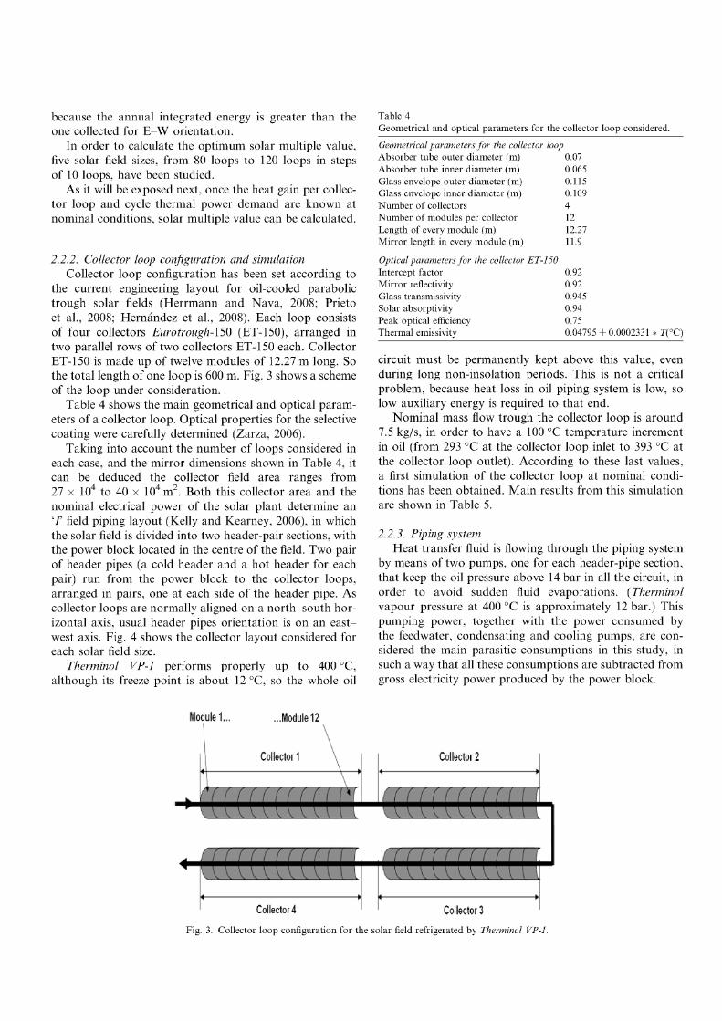
the current engineering layout for oil-cooled parabolic trough solar fields (Herrmann and Nava, 2008; Prieto et al., 2008; Hernández et al., 2008). Each loop consists of four collectors Eurotrough-150 (ET-150), arranged in two parallel rows of two collectors ET-150 each. Collector ET-150 is made up of twelve modules of 12.27 m long. So the total length of one loop is 600 m. Fig. 3 shows a scheme of the loop under consideration.

Table 4 shows the main geometrical and optical param-eters of a collector loop. Optical properties for the selective coating were carefully determined (Zarza, 2006).

Taking into account the number of loops considered in each case, and the mirror dimensions shown in Table 4, it can be deduced the collector field área ranges from 27 x 104 to 40 x 104m2. Both this collector área and the nominal electrical power of the solar plant determine an T field piping layout (Kelly and Kearney, 2006), in which the solar field is divided into two header-pair sections, with the power block located in the centre of the field. Two pair of header pipes (a cold header and a hot header for each pair) run from the power block to the collector loops, arranged in pairs, one at each side of the header pipe. As collector loops are normally aligned on a north-south hor­izontal axis, usual header pipes orientation is on an east-west axis. Fig. 4 shows the collector layout considered for each solar field size.

Therminol VP-1 performs properly up to 400 °C, although its freeze point is about 12 °C, so the whole oil

Table 4 Geometrical and optical parameters for the collector loop considered.

Geometrical parameters for the collector Absorber tube outer diameter (m) Absorber tube inner diameter (m) Glass envelope outer diameter (m) Glass envelope inner diameter (m) Number of collectors Number of modules per collector Length of every module (m) Mirror length in every module (m)

loop

Optical parameters for the collector ET-150 Intercept factor Mirror reflectivity Glass transmissivity Solar absorptivity Peak optical efficiency Thermal emissivity

0.07 0.065 0.115 0.109 4 12 12.27 11.9

0.92 0.92 0.945 0.94 0.75 0.04795 + 0.0002331 * r(°C)

circuit must be permanently kept above this valué, even during long non-insolation periods. This is not a critical problem, because heat loss in oil piping system is low, so low auxiliary energy is required to that end.

Nominal mass flow trough the collector loop is around 7.5 kg/s, in order to have a 100 °C temperature increment in oil (from 293 °C at the collector loop inlet to 393 °C at the collector loop outlet). According to these last valúes, a first simulation of the collector loop at nominal condi­tions has been obtained. Main results from this simulation are shown in Table 5.

2.2.3. Piping system Heat transfer fluid is flowing through the piping system

by means of two pumps, one for each header-pipe section, that keep the oil pressure above 14 bar in all the circuit, in order to avoid sudden fluid evaporations. (Therminol vapour pressure at 400 °C is approximately 12 bar.) This pumping power, together with the power consumed by the feedwater, condensating and cooling pumps, are con­sidered the main parasitic consumptions in this study, in such a way that all these consumptions are subtracted from gross electricity power produced by the power block.

.Module 12

Collector 1 \

r í í í i í í í í a \^[ -^v

( ( ( ( ( ( ( ( ( ( ( a {{{{{{{{{{[ i \

Collector 4

Collector 2

í(((ííí(íf{ 1 í umumiii f(((((((((11 Í {{{{[{[{{[{{{

Collector 3

Fig. 3. Collector loop configuration for the solar field refrigerated by Therminol VP-1.

West Field: Total number of loops: East Field:

40 l o o p s < 44 l o o p s * 50 l o o p s <

54 l o o p s < 60 l o o p s <

80 l oops > 40 l oops 90 l oops - > 46 l oops

100 l o o p s > 50 l oops

110 l o o p s > 56 l oops 120 l oops > 60 l oops

T_T L_J Í_J T_J T-X X_

Fig. 4. Collector field layout considered for the parabolic trough solar power plant.

Table 5 Simulation results for a collector loop refrigerated by Therminol VP-1, at the design-point conditions.

Simulation results Energy efficiency 70.23 Heat gain (MWth) 1.884 Heat loss (kWth) 178.4 Pressure drop (bar) 5.095 Mass flow per loop (kg/s) 7.725

Header pipes are needed to distribute the heat transfer fluid throughout the solar field. The chosen design for this piping system is based on maintaining the fluid velocity along the pipe length. This characteristic involves a theoretical pipe diameter modification every time the mass flow changes. If mass flow is going to a pair of loops, header pipe diameter decreases, whereas if mass flow is returning from a pair of loops, header pipe diameter increases. Actually, the number of different diameters is limited to three or four, depending on the solar field size, owing to constructive complexities.

On a first step, design velocity has been set to 2 m/s, both in the cold and hot header pipes. This valué has been

selected as a close-to-optimum design valué, according to Kelly and Kearney (2006). In sections between adjacent loops, a standard T pipe is used, in which the mass flow is sent to the loops; a sharply opening/contraction, where pipe diameter changes; and four 90° elbows, that conform a lira to absorb thermal expansions.

On a second step, three different commercial diameters have been adopted, for both the cold and hot header pipes, namely 10", 16" and 24", in such a way that flow velocity is almost always below 2 m/s. Pressure drop and heat loss resulting from these simulations are slightly greater than the ones obtained from theoretical diameters.

2.2.4. Solar múltiple calculation Table 6 shows solar múltiple calculation for each solar

field size considered. Thermal power required by the power block is the same in all the cases, as the power block is iden-tical for all the solar thermal power plants considered. Steam generator efficiency is also the same. However, both solar thermal power and piping system losses increase as the solar field size is larger.

Table 6 Solar múltiple for each parabolic trough plant considered.

Number of loops

80 90

100 110 120

Solar thermal (MW,„)

150.3 169.56 188.4 207.24 226.08

power Thermal losses in piping system (kWth)

417 491.3 568.8 650.1 734.4

Power block thermal demand (MWth)

142.6 142.6 142.6 142.6 142.6

Steam generator efficiency (%)

98 98 98 98 98

Solar múltiple (SM)

1.03 1.16 1.29 1.42 1.55

3. Annual simulation and economic analysis

Annual performance and economic analysis have been carried out for every solar field size. As a result, annual electricity production and cost of kWhe can be calculated and compared.

The following data are needed in order to calcúlate the annual balance of the solar thermal power plant:

- Direct normal irradiation valúes, at the plant location, with the required accuracy level. For this particular case, hourly valúes are precise enough.

- Part-load solar field performance, for different direct normal irradiation valúes.

- Part-load power block behaviour, for different electricity productions.

3.1. Direct normal irradiation valúes

Direct normal irradiation valúes have been obtained from Meteosat satellite images (Satel-Light, 2008), at the plant location, in Plataforma Solar de Almería site. Semi-hour valúes from five years (1996-2000) are available.

Because of direct irradiation data are referred to an hor­izontal surface, normal irradiation valúes have been obtained by calculations taking into account zenith angle valué in the centre of every semi-hour interval. Solar zenith and azimuth angle have been calculated according to Reda and Andreas (2003).

Besides that, in order to take into account that the par-abolic trough collector tracking system has only one degree of freedom (elevation) incidence angle for a N-S orienta-tion has been calculated, also in the middle of every semi-hour interval. This incident angle affects to the direct normal irradiation on the mirror aperture. This effect is accounted for the incident angle modifier for Eurotrough collector (Geyer et al., 2002):

K(6) = cos(0) - 2,859621 x 10~05 • 62 - 5,25097 x 10~04 • 9

(2)

In order to avoid atypical valúes of direct normal irradia­tion, data from Meteosat satellite have been compared with data from a typical meteorological year. This year has been established on the basis of a 22-years period (from July 1983 to June 2005). Monthly averaged valúes, as well as máx­imum and minimum valúes, are available in SSE datábase (Surface Meteorology and Solar Energy Project, 2008). Results from this study show that the five years selected can be considered within the limit valúes of the typical year.

3.2. Rankine steam cycle performance at part-load conditions

Part-load behaviour for the different power cycle com-ponents is needed to characterize power block performance

at part-load conditions, so the first part of this section is devoted to present the main equations characterizing part-load models.

Turbine efficiency will change at part load, compared to nominal conditions at full load. According to Bartlett (1958), the percent reduction in efficiency, as a function of the flow ratio, for the turbine considered:

% Reduction = 0.191 -0.409 • (m/mTeí) +0.218 • (m/mTeíf (3)

Is.turbme = (1 - % Reduction) • /íSiturbine.0 (4)

Steam turbine is controlled at part load by the sliding pressure method. This control method consists of main-taining turbine inlet temperature almost constant and decreasing turbine inlet pressure at part load. This method is preferred to valve control method because it is better adapted to large load changes, although valve control method presents better efficiency at slight load changes (Muñoz Torralbo et al., 2001). Pressure drop over a turbine stage is calculated by means of the following law (Stodola and Loewenstein, 1945):

^-^ = f A Y (5)

Generator efficiency is a function of the ratio between current and nominal electricity power. This efficiency vari-ation ranges from 92.5% to 98% approximately. For this study, SEGS VI generator efficiency variation has been adopted (Patnode, 2006):

generator = 0-908+ 0.258 • Load - 0.3 • Load2+ 0.12 • Load3

(6)

As it was said in Section 2, all the heat exchangers in the cycle, except the deaerator, are characterized by means of their overall heat transfer coefficient and their efficiency. In a first approximation (Patnode, 2006), overall heat transfer coefficient changes at part load following:

Eq. (7) is an estimation obtained on the basis of consid-ering Dittus-Boelter correlation for forced convection in circular pipes (Rohsenow et al., 1998).

Pressure drop of every stream in all heat exchangers is proportional to the square of the mass flow:

AP = kP-m2 (8)

As a first order estimation, kp is assumed to be constant and it is calculated based on the pressure drop known at nominal conditions.

Regarding pumps, isentropic efficiency also changes at part-load conditions. Assuming that the pumps opérate at máximum efficiency at nominal conditions, the change in pump efficiency is expressed as a function of the mass flow ratio (Lippke, 1995):

s.pump . = gm0 + 2 • (1 - em0) • -^— - (1 - em0) Vs,pump_0

m m

(9)

em0 is a parameter defining the shape of the efficiency curve. Its valué is zero for constant speed pumps, hypothesis as-sumed for all the pumps in this study.

Once the main equations characterizing part-load behaviour of the power block components are imple-mented, cycle efficiency and thermal power required in the steam generator and reheater, at different part load, are calculated. Results are shown in Fig. 5.

Steam generator efficiency (98%) will be taken into account when global and annual parabolic trough plant balances were performed. Electricity power consumption as a function of the load presents a quadratic shape varia-tion in all the pumps.

3.3. Solar thermal power under different direct normal irradiation valúes

Results obtained in this way are more accurate, because incidence angle valué is obtained in every simulation step.

Thermal power for the different solar field sizes consid-ered has been represented in Fig. 6. It can be seen that solar thermal power depends linearly on the incident direct solar irradiation. For this reason, solar thermal power can be modelled by a first-order polynomial function of direct normal irradiation, the coefficients of which are obtained by linear regression. These functions are summarized in Table 7.

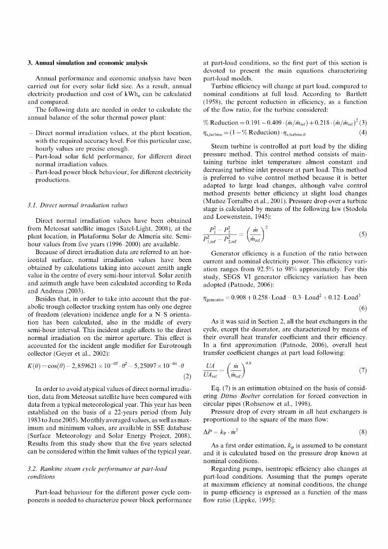
Fig. 7 shows solar field thermal efficiency at part load. This curve has been obtained considering that optical parameters valúes remain constant (equal to design-point valúes), and only DNI changes from 300 to 950 W/m2. In this case, there is no a linear dependency on direct normal irradiation; efficiency decreases 3% from 950 to 550 W/m2, whereas it decreases more steeply (6%) from 550 to 300 W/ m2, because heat gain per collector drastically decreases for these valúes. Overall power plant efficiency calculation requires optical and geometrical efficiencies estimation. Such efficiencies mainly depend on the optics at every

In this section, solar field performance has been obtained under different direct normal irradiation (DNI) valúes. Under certain assumptions, the optimum strategy is based on adapting the solar fluid outlet temperature to the solar power, keeping the mass flow cióse to constant (Lippke, 1995). In this paper, a different approach has been adopted, and the solar fluid outlet temperature has been kept constant. The mass flow has been adapted to the solar power. This strategy is also simpler to implement in the hourly simulation used in this paper. For future works, with a higher accuracy in the turbine simulation for off-nominal conditions, a correlation can be adopted between the solar power and the optimum turbine power, and the hourly simulation can be adapted to it.

Incidence angle effect must be considered, but the strat­egy adopted for the annual balance requires incidence angle calculation in the centre of every half-hour interval.

38

36

34-|

32

30

28-|

26

24

y

S y y y

y y

y y -m- Power block efficiency

Thermal power supplied to steam generator and reheater

160

140

-120 j (D

100 |

•o 80 |

IB

60 Z

40 $

20 20 40 60

Load(%) 80 100

Fig. part

5. Power block efficiency and thermal power supplied to the BOP at load.

300

250

<l>

s Q.

"¡5 p i) ^ i—

•o

o u. Ü o

200

150

100

50

(O

350 450 550 650 750 850 950

DNI (W/m

Fig. 6. Solar field thermal power at part load, for the different solar múltiples considered. For this collection incident angle of solar radiation has not been taken into account. This angle will be applied later, in annual balance.

Table 7 Solar field thermal power as a function of the incident direct normal irradiation.

Thermal power for different solar field sizes

Solar múltiple (SM) Thermal power (MWjJ

1.04

1.17

1.29

1.42

1.55

Thermal power (MWth) = 0.198 * DNI (W/m2) - 10.737 ^vv/m ) — I U . / J ;

Thermal power (MWth) = 0.2228 * DNI (W/m2) - 12.08 Thermal power (MWth) = 0.2475 * DNI (W/m2) - 13.422 Thermal power (MWth) = 0.2723 * DNI (W/m2) - 14.764 Thermal power (MWth) = 0.297 * DNI (W/m 2 ) - 16.106

72-

>, 70 u c di

1 68

di E 66-di .c 2 64 ai

re 62 o

60

Thermal efficiency for an ¡ncidence angle = 13°39'14.4" (design-point valué)

— I —

350 — i —

450 550 650

DNIfW/m 2 )

— i — 750

— i —

850 950

Fig. 7. Solar field thermal efficiency as a function of the direct normal irradiation.

moment, as well as collector shading and end losses, so they will be calculated at every simulation time step in the annual balance.

Expressions to estimate shading and end losses have been obtained by basic trigonometrical analysis (Stuetzle, 2002). Shading effect between adjacent collector rows is estimated assuming that the effective width of the collector is the non-shaded part of the collector width. Effective width is a function of distance between adjacent collector rows, mirror width, zenith and incident angle. On the other hand, end losses are function of the focal length of the col-lector and the incidence angle.

Another important issue is mirror reflectivity change owing to dirt effect. Dirt on mirrors mainly depends on fre-quency of cleaning adopted within plant operation and maintenance strategy. According to Cohén et al. (1999), a good assumption for mirrors wash cycles is considering an annual averaged reflectivity valué, 2% below design-point valué.

3.4. Economic analysis

Once annual electricity production is estimated, eco­nomic analysis may be performed to calcúlate the cost of the kWhe, that is, the levelized cost of energy (LCOE), defined in

LCOE fcr • Cir Cc Cfi (10)

where fcr is the annuity factor (9.88%); Cinvest (million euros), total investment of the plant; CO&M (million euros) annual operation and maintenance costs; Cfuei (million euros) annual fuel costs; and Enet, annual net electric en­ergy produced. For this particular case, annual fuel costs are nuil, because a solar-only plant, without hybridization, has been considered.

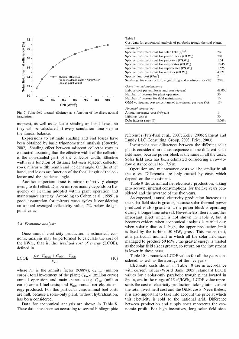
Data for economical analysis are shown in Table 8. These data have been set according to several bibliographic

Table 8 Cost data for economical analysis of parabolic trough thermal plants.

Investment Specific investment cost for solar field (€/m2) Specific investment cost for power block (€/kWe) Specific investment cost for preheater (€/kWe) Specific investment cost for evaporator (€/kWe) Specific investment cost for superheater (€/kWe) Specific investment cost for reheater (€/kWe) Specific land cost (€/m2) Surcharge for construction, engineering and contingencies (%)

Operation and maintenance Labour cost per employee and year (€/year) Number of persons for plant operation Number of persons for field maintenance O&M equipment cost percentage of investment per year (%)

Financial parameters Annual insurance cost (%/year) Lifetime (years) Debt interest rate (%)

206 700 1.54 10.45 1.625 4.221 2 20%

48,000 30 10 1%

1 30 8.00%

references (Pitz-Paal et al., 2007; Kelly, 2006; Sargent and Lundy LLC Consulting Group, 2003; Price, 2003).

Investment cost differences between the different solar plants considered are a consequence of the different solar field sizes, because power block is the same in all the cases. Solar field área has been estimated considering a row-to-row distance equal to 17.5 m.

Operation and maintenance costs will be similar in all the cases. Differences are only caused by costs which depend on the investment.

Table 9 shows annual net electricity production, taking into account internal consumptions, for the five years con­sidered and the average of the five years.

As expected, annual electricity production increases as the solar field size is greater, because solar thermal power produced is also greater and the power block is operating during a longer time interval. Nevertheless, there is another important effect which is not shown in Table 9, but it becomes evident when economical analysis is carried out: when solar radiation is high, the upper production limit is fixed by the turbine: 50 MWe gross. This means that, at a particular moment in which all the solar field sizes managed to produce 50 MWe, the greater energy is wasted as the solar field size is greater, so return on the investment is lower in these cases.

Table 10 summarizes LCOE valúes for all the years con­sidered, as well as the average of the five years.

Electricity costs shown in Table 10 are in accordance with current valúes (World Bank, 2005); standard LCOE valúes for a solar-only parabolic trough plant located in Spain, are in the range of 15 c€/kWhe. LCOE valué repre-sents the cost of electricity production, taking into account the total investment cost and the O&M costs. Nevertheless, it is also important to take into account the price at which this electricity is sold to the national grid. Difference between production and supply costs represents the eco­nomic profit. For high incentives, long solar field sizes

Table 9

Annua l net electricity product ion for every solar múltiple and every year considered.

Parabolic t rough solar field

Solar múltiple (SM)

1.03

1.16

1.29

1.42

1.55

Annua l net

1996

101.84

110.4

116.63

121.35

124.99

electricity product ion

1997

102.86

111.53

117.47

122.03

125.55

(GWh e )

1998

107.19

116.06

122.26

127.09

130.89

1999

111.98

120.38

126.26

130.64

134.08

2000

110.75

119.92

126.39

131.24

134.99

Average

106.924

115.658

121.802

126.47

130.1

Table 10

Levelized cost of energy for every solar múltiple and every year considered.

Parabolic t rough solar field

Solar múltiple

1.03

1.16

1.29

1.42

1.55

L C O E

1996

14.138

13.92

14.008

14.263

14.623

(c€/kWh e)

1997

13.998

13.778

13.908

14.183

14.557

1998

13.433

13.241

13.363

13.618

13.964

1999

12.858

12.766

12.939

13.248

13.632

2000

13.001

12.815

12.926

13.188

13.54

Average

13.486

13.304

13.429

13.700

14.063

result more profitable, whereas if the prime is next to the electricity production cost, LCOE valúes must be consid­ered. LCOE valúes are also represented in Fig. 8.

As can be observed in Fig. 8, average LCOE valué is minimum for a certain solar field size. In this case, this size is the one corresponding to a solar múltiple of 1.16, with a solar field consisting of 90 loops. Nevertheless, it is worth pointing out that this cost estimation has been done on the basis of a referenced economic data. It is clear that the absolute LCOE valué will depend on the investment and O&M costs for every particular case.

4. Sensitivity analysis: influence of several parameters on the optimum solar múltiple valué

As it was said in Section 1, optimum solar múltiple valué depends not only on the solar field size, but also on the design-point conditions, solar plant location, solar field and power block characteristics. In this way, solar múltiple

14.10-

~ Í 13.95-1 .C

¿S 13.80

_ü_

UJ 13.65 O O "" 13.50

13.35

13.20

Average LCOE

1.0 1.1 1.2 1.3 1.4

S o l a r Múltiple

1.5 1.6

expression shows that the more efficient the power cycle is the lower solar field área is necessary to produce the same electrical power.

This last influence parameter has been studied in more detail by means of annual simulations for a case with the same plant location and design point, but with different power cycle configuration, using four extractions from the turbine instead of 6.

Nominal parameters of this new cycle have been chosen similar to those adopted for the regenerative six-extractions cycle (Table 1). Nevertheless, because of the number of extractions, nominal thermal power in the steam generator is higher in the case of four extractions, so cycle efficiency is lower. Both parameters are displayed in Fig. 9.

Fig. 10 shows the average LCOE valué of the annual simulations for the five years considered. The result obtained for the case analyzed in Section 3 (power block with six heat exchanger feeders) has also been represented.

38

36

34

32 ü a 30

¡C 28 LU

26

24

22

/ • • ^

• y*

/ / ' / o - • - Power block efficiency / - • - Thermal power supplied to steam

• generator and reheater

-140

-120

-100

-80

-60

-40

-20

I

20 40 60 Load(%)

80 100

Fig. 8. Electricity cost for every solar múltiple and every year considered. Fig. 9. Power block efficiency and thermal power supplied to the BOP at part load.

14.2

£ » 14.0 g je

* 13.8

Average LCOE for Power Block 2

Average LCOE for Power Block 1

1.2 1.4 Solar Múltiple

1.6

Fig. 10. Average electricity cost of the five years for every solar múltiple considered and two configurations of the power block.

It can be observed that LCOE valúes for the case of a power block with four extraction points are higher than the previous one. It can be also observed that the optimum solar múltiple is slightly higher than the one obtained in Section 3. Both facts are a consequence of the less efficient power cycle and they make it evident that an improved power block may suppose larger savings in the investment.

5. Conclusions

This paper presents a standard methodology for the eco-nomic optimization of the solar múltiple in parabolic trough plants. Although the study has been focused on a conventional synthetic oil parabolic trough plant, with no storage or hybridization, this approach can be extended to more complex solar thermal plants designs.

The first step in this methodology is the thermal behav-iour calculation of the different systems included in the solar power plant, both at nominal and part load. As this study is based on annual performance simulations, it is essential to characterize the optical losses in every moment. In this case, optical losses are taken into account by means of the incidence angle and the incidence angle modifier. Once the annual electricity production is calculated for each of the parabolic trough plant sizes considered, the economic analysis may be accomplished. As a result of this analysis, optimum solar múltiple is obtained, i.e., solar field size for which LCOE valué is minimal is obtained.

In this particular case optimum solar múltiple valué is 1.16. For thermal plants without thermal storage, as the case of the study, the solar múltiple must be large enough to ensure a certain range where the solar thermal plant is operating at nominal conditions, but it should not be very great. In this last case, large sizes of solar fields without thermal storage would achieve a worse return on their investment, as solar thermal energy above nominal level would be wasted. It should be pointed out that this opti­mum valué has been obtained assuming that there is no a

peak demand period where the electricity price might be affected by a tariff-based incentive. In such a case, the elec­tricity production interval should be also taken into account.

This work also presents that optimum solar múltiple depends on several factors. In particular, the last analysis in Section 4 shows that improving the efficiency by means of more complex power cycles leads to significant invest­ment savings in the solar field size.

References

Bartlett, R.L., 1958. Steam Turbine Performance and Economics. McGraw-Hill, New York, USA, pp. 70-109. LCCCN: 58-8039.

Cohén, E.G. et al., 1999. Final Report on the Operation and Maintenance Improvement Program for Concentrating Solar Power Plants. Report No. SAND99-1290, SNL, Alburquerque, NM, USA.

Geyer, M. et al., 2002. EUROTROUGH - parabolic trough collector developed for cost efficient solar power generation. In: Proceedings of l lst International Symposium on Concentrating Solar Power and Chemical Energy Technologies, Zurich, Switzerland.

Hernández, C. et al., 2008. Iberdrola renewables and solar thermal technologies. In: Proceedings of 14th International SolarPACES Symposium on Solar Thermal Concentrating Technologies, Las Vegas, USA.

Herrmann, U , Nava, P., 2008. Performance of the SKAL-ET collector of the Andasol power plants. In: Proceedings of 14th International SolarPACES Symposium on Solar Thermal Concentrating Technol­ogies, Las Vegas, USA.

Kelly, B., 2006. Nexant Parabolic Trough Solar Power Systems Analysis. Task 1: Preferred Plant Size. Report No. NREL/SR-550-40162, NREL, Colorado, USA.

Kelly, B., Kearney, D., 2006. Parabolic Trough Solar System Piping Model. Report No. NREL/SR-550-40165, NREL, Colorado, USA.

Kostyuk, A., Frolov, V., 1988. Steam and Gas Turbines. Mir, Moscow, Russia. ISBN 5-03-000032-1.

Lippke, F., 1995. Simulation of the Part-Load Behaviour of a 30 MWe SEGS Plant. Report No. SAND95-1293, SNL, Alburquerque, NM, USA.

Muñoz Torralbo, M., Valdés del Fresno, M., Muñoz Domínguez, M., 2001. Turbomáquinas térmicas: fundamentos del diseño termodinám-ico. E.T.S. de Ingenieros Industriales, Universidad Politécnica de Madrid, Spain, pp. 330-347. ISBN 84-7484-143-7.

Patnode, A.M., 2006. Simulation and Performance Evaluation of Para­bolic Trough Solar Power Plants. Ph.D. Thesis, University of Wisconsin-Madison, USA.

Pitz-Paal, R. et al., 2007. Development steps for parabolic trough solar power technologies with máximum impact on cost reduction. Journal of Solar Energy Engineering 129 (4), 371-377.

Price, H., 2003. A Parabolic Trough Solar Power Plant Simulation Model. Report No. NREL//CP-550-33209, NREL, Colorado, USA.

Price, H. et al., 2002. Advances in parabolic trough solar power technology. Journal of Solar Energy Engineering 124 (2), 109-125.

Prieto, C. et al., 2008. Parabolic trough technology in abengoa solar. In: Proceedings of 14th International SolarPACES Symposium on Solar Thermal Concentrating Technologies, Las Vegas, USA.

Quaschning, V., Kistner, R., Ortmanns, W., 2002. Influence of direct normal irradiance variation on the optimal parabolic trough field size: a problem solved with technical and economical simulations. Journal of Solar Energy Engineering 124, 160-164.

Reda, I., Andreas, A., 2003. Solar Position Algorithm for Solar Radiation Applications. Technical Report NREL/TP-560-34302, Colorado, USA.

Relloso, S., Gutiérrez, Y., 2008. Real application of molten salt thermal storage to obtain high capacity factors in parabolic trough plants. In:

Proceedings of 14th International SolarPACES Symposium on Solar Thermal Concentrating Technologies, Las Vegas, USA.

Rohsenow, W.M., Hartnett, J.P., Cho, Y.I., 1998. Handbook of Heat Transfer, third ed. McGraw-Hill, New York, USA. ISBN 0070535558.

Sargent and Lundy LLC Consulting Group, 2003. Assessment of Parabolic Trough and Power Tower Solar Technology Cost and Performance Forecasts. Report No. NREL/SR-550-34440, NREL, Colorado, USA.

Satel-Light, 2008. Available from www.satel-light.com. Stodola, A., Loewenstein, L.C., 1945. In: Steam and Gas Turbines, vol. I.

McGraw-Hill Book Company, New York, USA.

Stuetzle, T., 2002. Automatic Control of the 30 MWe SEGS VI Parabolic Trough Plant. Ph.D. Thesis, University of Wisconsin-Madison, USA.

Surface Meteorology and Solar Energy Project, 2008. Available from: http://eosweb.larc.nasa.gov/sse/.

World Bank, 2005. Assessment of the World Bank/GEF Strategy for the Market Development of Concentrating Solar Thermal Power. Report No. GEF/C.25/Inf.ll, Global Environment Facility, Washington, USA.

Zarza, E., 2006. Personal Communication. Plataforma Solar de Almería. Available from: http://www.psa.es.