1 Solid State Physics Lecture notes by Michael Hilke McGill University (v. 10/25/2006) Contents Introduction 2 The Theory of Everything 3 H 2 O - An example 3 Binding 3 Van der Waals attraction 3 Derivation of Van der Waals 3 Repulsion 3 Crystals 3 Ionic crystals 4 Quantum mechanics as a bonder 4 Hydrogen-like bonding 4 Covalent bonding 5 Metals 5 Binding summary 5 Structure 6 Illustrations 6 Summary 6 Scattering 6 Scattering theory of everything 7 1D scattering pattern 7 Point-like scatterers on a Bravais lattice in 3D 7 General case of a Bravais lattice with basis 8 Example: the structure factor of a BCC lattice 8 Bragg’s law 9 Summary of scattering 9 Properties of Solids and liquids 10 single electron approximation 10 Properties of the free electron model 10 Periodic potentials 11 Kronig-Penney model 11 Tight binging approximation 12 Combining Bloch’s theorem with the tight binding approximation 13 Weak potential approximation 14 Localization 14 Electronic properties due to periodic potential 15 Density of states 15 Average velocity 15 Response to an external field and existence of holes and electrons 15 Bloch oscillations 16 Semiclassical motion in a magnetic field 16 Quantization of the cyclotron orbit: Landau levels 16 Magneto-oscillations 17 Phonons: lattice vibrations 17 Mono-atomic phonon dispersion in 1D 17 Optical branch 18 Experimental determination of the phonon dispersion 18 Origin of the elastic constant 19 Quantum case 19 Transport (Boltzmann theory) 21 Relaxation time approximation 21 Case 1: ~ F = -e ~ E 21 Diffusion model of transport (Drude) 22 Case 2: Thermal inequilibrium 22 Physical quantities 23 Semiconductors 24 Band Structure 24 Electron and hole densities in intrinsic (undoped) semiconductors 25 Doped Semiconductors 26 Carrier Densities in Doped semiconductor 27 Metal-Insulator transition 27 In practice 28 p-n junction 28 One dimensional conductance 29 More than one channel, the quantum point contact 29 Quantum Hall effect 30 superconductivity 30 BCS theory 31
Transcript
1
Solid State PhysicsLecture notes byMichael Hilke
McGill University(v. 10/25/2006)
Contents
Introduction 2
The Theory of Everything 3
H2O - An example 3
Binding 3Van der Waals attraction 3Derivation of Van der Waals 3Repulsion 3Crystals 3Ionic crystals 4Quantum mechanics as a bonder 4Hydrogen-like bonding 4Covalent bonding 5Metals 5
Binding summary 5
Structure 6Illustrations 6Summary 6
Scattering 6Scattering theory of everything 71D scattering pattern 7Point-like scatterers on a Bravais lattice in 3D 7General case of a Bravais lattice with basis 8Example: the structure factor of a BCC lattice 8Bragg’s law 9Summary of scattering 9
Properties of Solids and liquids 10single electron approximation 10Properties of the free electron model 10
Periodic potentials 11Kronig-Penney model 11Tight binging approximation 12Combining Bloch’s theorem with the tight bindingapproximation 13Weak potential approximation 14Localization 14
Electronic properties due to periodic potential 15Density of states 15Average velocity 15Response to an external field and existence of holesand electrons 15Bloch oscillations 16
Semiclassical motion in a magnetic field 16Quantization of the cyclotron orbit: Landau levels 16Magneto-oscillations 17
Phonons: lattice vibrations 17Mono-atomic phonon dispersion in 1D 17Optical branch 18Experimental determination of the phonondispersion 18Origin of the elastic constant 19Quantum case 19
Transport (Boltzmann theory) 21Relaxation time approximation 21Case 1: ~F = −e ~E 21Diffusion model of transport (Drude) 22Case 2: Thermal inequilibrium 22Physical quantities 23
Semiconductors 24Band Structure 24Electron and hole densities in intrinsic (undoped)semiconductors 25Doped Semiconductors 26Carrier Densities in Doped semiconductor 27Metal-Insulator transition 27In practice 28p-n junction 28
One dimensional conductance 29
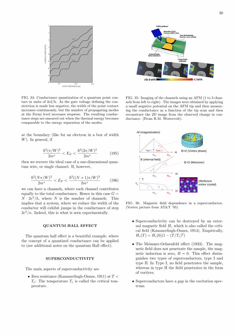
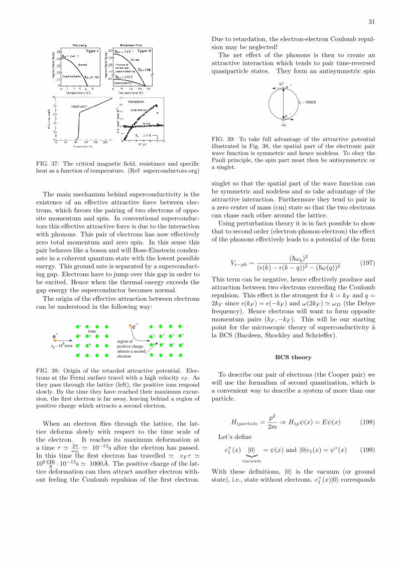
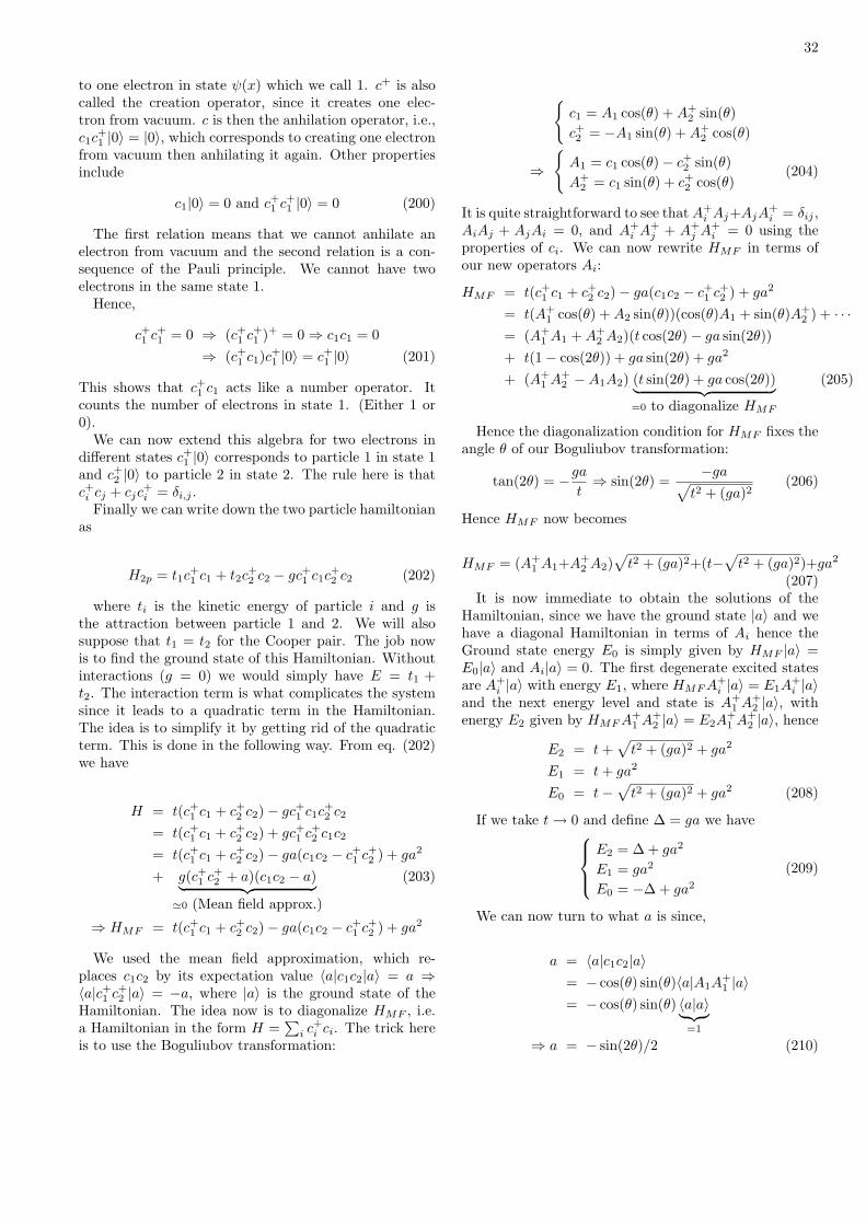
More than one channel, the quantum pointcontact 29
Quantum Hall effect 30
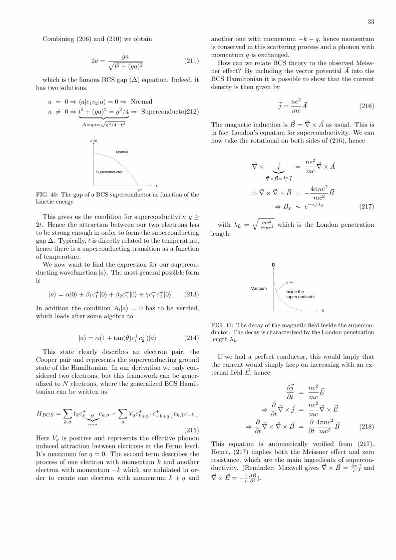
superconductivity 30BCS theory 31
2
INTRODUCTION
What is Solid State Physics?Typically properties related to crystals, i.e., period-
icity.What is Condensed Matter Physics?
Properties related to solids and liquids including crys-tals. For example: liquids, polymers, carbon nanotubes,rubber,...
Historically, SSP was considers as he basis for the un-derstanding of solids since many of the properties were
derived based on a periodic lattice. However it appearedthat most of the properties are very similar independentof the presence or not of a lattice. But there are manyexceptions, for example, localization due to disorder orthe disappearance of the periodicity.
Even in crystals, liquid-like properties can arise, suchas a Fermi liquid, which is an interacting electron system.The same is also true the other way around since liquidscan form liquid crystals.
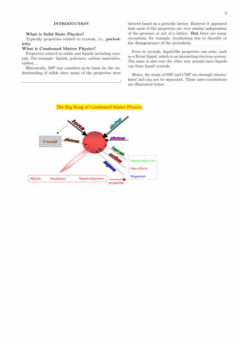
Hence, the study of SSP and CMP are strongly interre-lated and can not be separated. These inter-correlationsare illustrated below.
Crystal
Supraconductivity Opto-effects Magnetism
Crystal
Metals Insulators Semiconductors properties
The Big Bang of Condensed Matter Physics
3
THE THEORY OF EVERYTHING
See ppt notes
H2O - AN EXAMPLE
See ppt notes
BINDING
What holds atoms together and also keeps them fromcollapsing?
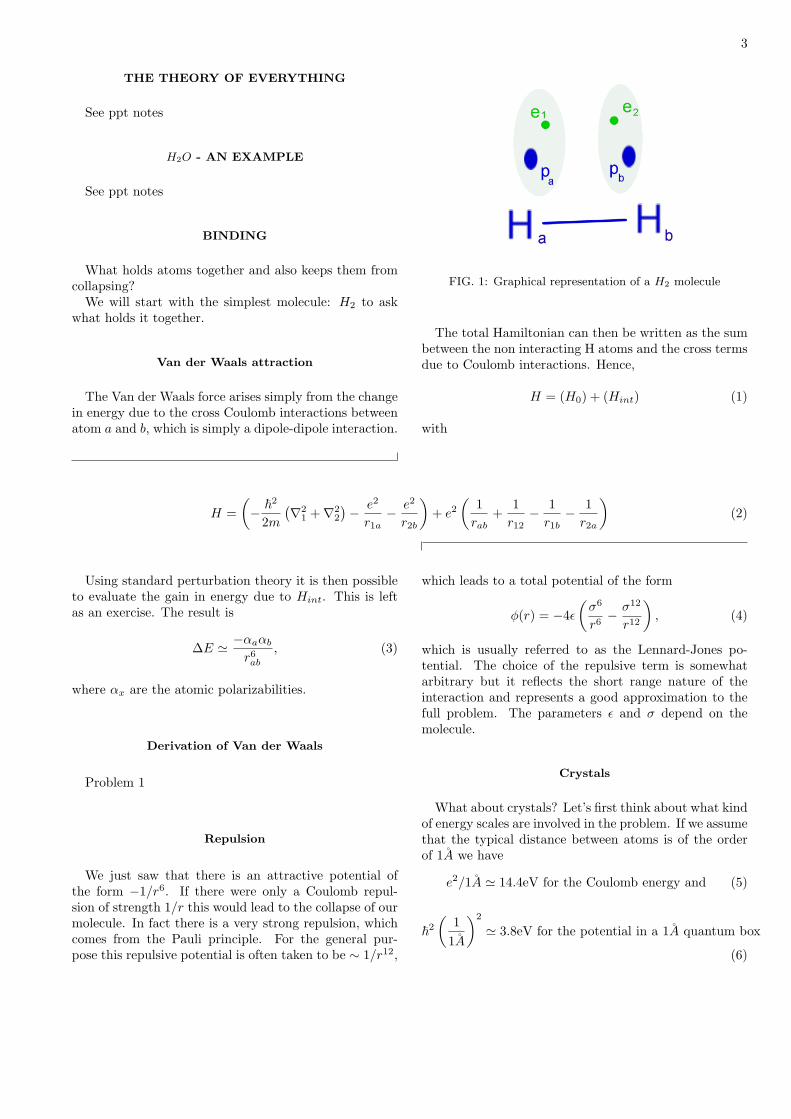
We will start with the simplest molecule: H2 to askwhat holds it together.
Van der Waals attraction
The Van der Waals force arises simply from the changein energy due to the cross Coulomb interactions betweenatom a and b, which is simply a dipole-dipole interaction.
FIG. 1: Graphical representation of a H2 molecule
The total Hamiltonian can then be written as the sumbetween the non interacting H atoms and the cross termsdue to Coulomb interactions. Hence,
H = (H0) + (Hint) (1)
with
H =(− ~
2
2m
(∇21 +∇2
2
)− e2
r1a− e2
r2b
)+ e2
(1
rab+
1r12
− 1r1b
− 1r2a
)(2)
Using standard perturbation theory it is then possibleto evaluate the gain in energy due to Hint. This is leftas an exercise. The result is
∆E ' −αaαb
r6ab
, (3)
where αx are the atomic polarizabilities.
Derivation of Van der Waals
Problem 1
Repulsion
We just saw that there is an attractive potential ofthe form −1/r6. If there were only a Coulomb repul-sion of strength 1/r this would lead to the collapse of ourmolecule. In fact there is a very strong repulsion, whichcomes from the Pauli principle. For the general pur-pose this repulsive potential is often taken to be ∼ 1/r12,
which leads to a total potential of the form
φ(r) = −4ε
(σ6
r6− σ12
r12
), (4)
which is usually referred to as the Lennard-Jones po-tential. The choice of the repulsive term is somewhatarbitrary but it reflects the short range nature of theinteraction and represents a good approximation to thefull problem. The parameters ε and σ depend on themolecule.
Crystals
What about crystals? Let’s first think about what kindof energy scales are involved in the problem. If we assumethat the typical distance between atoms is of the orderof 1A we have
e2/1A ' 14.4eV for the Coulomb energy and (5)
~2
(1
1A
)2
' 3.8eV for the potential in a 1A quantum box
(6)
4
In comparison to room temperature (300K' 25meV)these energies are huge. Hence ionic Crystals like NaClare extremely stable, with binding energies of the orderof 1eV.
Ionic crystals
Some solids or crystals are mainly held together by theelectrostatic potential and they include the alkali-halideslike (NaCl −→ Na+Cl−).
+ -
d
FIG. 2: A simple ionic crystal such as NaCl
The energy per ion pair is
Energy
Nionpair= −α
e2
d+
C
dn= −α
14.4eV
[d/A]+
C
dnwith 6 < n ≤ 12,
(7)where α is the Madelung constant and can be calcu-
lated from the crystal structure. C can be extracted ex-perimentally from the minimum in the potential energyand typically n = 12 is often used to model the effectof the Pauli principle. Hence, from the derivative of thepotential we obtain:
d0 =(
12C
e2α
)1/11
(8)
so that
Energy
Nionpair=
11αe2
12d0(9)
How good is this model? See table below:
Quantum mechanics as a bonder
Hydrogen-like bonding
Let’s start with one H atom. We fix the proton atr = o then we know form basic quantum mechanics that
the ground state energy is then given by E0=-13.6 eV.What happens if we add one proton or H+ to the systemwhich is R away. The potential energy for the electron isthen
U(r) = −e2
r− e2
|r −R| (10)
The lowest eigenfunction with eigenvalue -13.6eV is
ξ(r) =1√π
(1a0
)3/2
e−r/a0 , (11)
where a0 is the Bohr radius. But now we have twoprotons. If the protons were infinitely apart then thegeneral solution to potential 10 is a linear superposi-tion ,i.e., ψ(r) = αξ(r) + βξ(r − R) with a degener-ate lowest eigenvalue of E0 = E0=-13.6 eV. When Ris not infinite, the two eigenfunctions corresponding tothe lowest eigenvalues Eb and Ea can be approximatedby ψb = ξ(r) + ξ(r − R) and ψa = ξ(r) − ξ(r − R). Seefigure 3.
0
0Ψ
a(r)V(r)
Ψb(r)
+ +R
r
FIG. 3: The potential for two protons with the bonding andanti-binding wave function of the electron
The average energy (or expectation value of Eb) is
Eb = 〈ψ∗b Hψb〉/〈ψ∗b ψb〉 (12)
= E0 − A + B
1 + ∆with (13)
A = e2
∫drξ2(r)/|r −R| (14)
B = e2
∫drξ(r)ξ(|r −R|)/r (15)
∆ =∫
drξ(r)ξ(|r −R|), (16)
where 〈·〉 ≡ ∫ ·dr and similarly,
Ea = E0 − A−B
1−∆(17)
5
Hence, the total energy for state ψb is now
Etotalb = Eb + e2/R (18)
When plugging in the numbers Etotalb has a minimum at
1.5A. See figure 4
-16
-12
-8
R0
Antibonding
Ea
Eb
Eb
tot
Ea
tot
Bonding
R [distance between protons]
-13.6 eVE [e
V]
FIG. 4: The energies as a function of the distance betweenthem for the bonding and anti-binding wave functions of theelectron
This figure illustrates why they are called bonding andanti-bonding, since in the bonding case the energy is low-ered when the distance between protons is reduced aslong as R > R0.
Covalent bonding
Covalent bonds are very similar to Hydrogen bonds,only that we have to extend the problem to a linear com-bination of atomic orbitals for every atom. N atomswould lead to N levels, in which the ground state has abonding wave-function.
Metals
In metals bonding is a combination of the effects dis-cussed above. The idea is to consider a cloud of electronsonly weakly bound to the atomic lattice. The total elec-trostatic energy can then be written as
Eel = −∫
drn(r)∑
R
e2
r −R+
∑
R>R′
e2
R−R′+ 1/2 ·
∫dr1dr2
e2n(r1)n(r2)|r1 − r2| (19)
which corresponds to an ionic contribution of the form
Eel = −αe2
2rswhere rs =
(3
4πn
)1/3
(20)
and α is the Madelung constant. Deriving this requiresquite a bit of effort. On top of this one has to add thekinetic energy of the electrons, which is of the form:
Ekin =(
9π
4
)2/3 3~2
10mr2s
(21)
And finally we have to add the exchange energy, with isa consequence of the Pauli principle. The expression forthis term is given by
Eex = −(
9π
4
)1/3 34πrs
(22)
Putting all this together we obtain in units of the Bohrradius:
E =(−24.35a0
rS+
30.1a20
r2S
− 12.5a0
rs
)eV/atom (23)
This last expressions leads to a minimum at rs/a0 = 1.6.We can now compare this with experimental values andthe result is off by a factor between 2 and 6. What wentwrong. Well, we treated the problem on a semiclassi-cal level, without incorporating all the electron-electroninteractions in a quantum theory. This is very very diffi-cult, but in the large density case this can be estimatedand a better agreement with experiments is obtained.
Binding summary
There are essentially three effects which contribute tothe binding of solids:
• Van der Waals (a dipole-dipole like interaction)
• ionic (Coulomb attraction between ions)
• Quantum mechanics (overlap of the wave-function)
In addition we have two effects which prevent the collapseof the solids:
6
• Coulomb
• Quantum mechanics (Pauli)
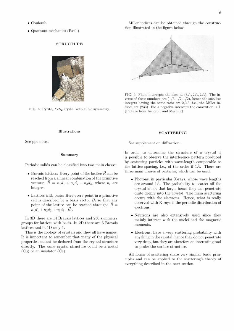
STRUCTURE
FIG. 5: Pyrite, FeS2 crystal with cubic symmetry.
Illustrations
See ppt notes.
Summary
Periodic solids can be classified into two main classes:
• Bravais lattices: Every point of the lattice ~R can bereached from a a linear combination of the primitivevectors: ~R = n1a1 + n2a2 + n3a3, where ni areintegers.
• Lattices with basis: Here every point in a primitivecell is described by a basis vector ~Bi so that anypoint of the lattice can be reached through: ~R =n1a1 + n2a2 + n3a3+ ~Bi.
In 3D there are 14 Bravais lattices and 230 symmetrygroups for lattices with basis. In 2D there are 5 Bravaislattices and in 1D only 1.
This is the zoology of crystals and they all have names.It is important to remember that many of the physicalproperties cannot be deduced from the crystal structuredirectly. The same crystal structure could be a metal(Cu) or an insulator (Ca).
Miller indices can be obtained through the construc-tion illustrated in the figure below:
FIG. 6: Plane intercepts the axes at (3a1, 2a2, 2a3). The in-verse of these numbers are (1/3, 1/2, 1/2), hence the smallestintegers having the same ratio are 2,3,3, i.e., the Miller in-dices are (233). For a negative intercept the convention is 1.(Picture from Ashcroft and Mermin)
SCATTERING
See supplement on diffraction.
In order to determine the structure of a crystal itis possible to observe the interference pattern producedby scattering particles with wave-length comparable tothe lattice spacing, i.e., of the order if 1A. There arethree main classes of particles, which can be used:
• Photons, in particular X-rays, whose wave lengthsare around 1A. The probability to scatter off thecrystal is not that large, hence they can penetratequite deeply into the crystal. The main scatteringoccurs with the electrons. Hence, what is reallyobserved with X-rays is the periodic distribution ofelectrons.
• Neutrons are also extensively used since theymainly interact with the nuclei and the magneticmoments.
• Electrons, have a very scattering probability withanything in the crystal, hence they do not penetratevery deep, but they are therefore an interesting toolto probe the surface structure.
All forms of scattering share very similar basic prin-ciples and can be applied to the scattering’s theory ofeverything described in the next section.
7
Scattering theory of everything
← crystal
Incidentbeam Outgoing
beam
rk ⋅'ierk⋅ie
ϕϕϕϕr
dV
kk’
O
[ ]
'-
)(d)( 3
kkq
rrq rq
=
⋅∝ ⋅∫∫∫ i
V
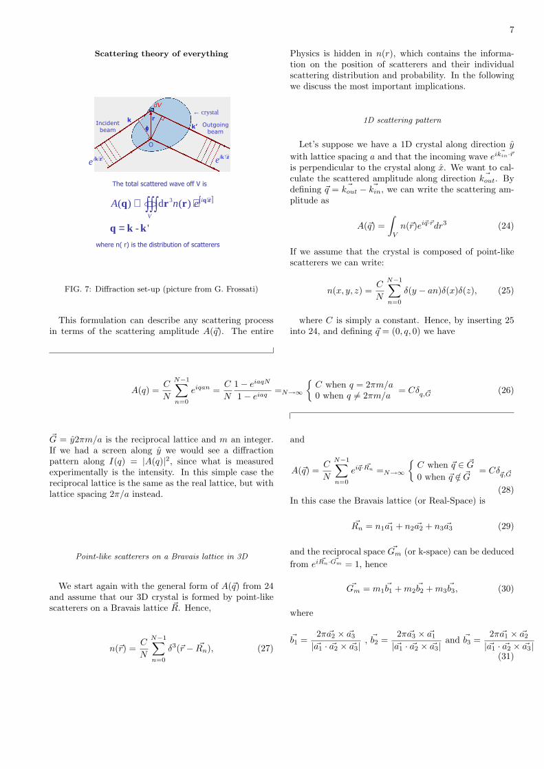
enA
where n( r) is the distribution of scatterers
The total scattered wave off V is
FIG. 7: Diffraction set-up (picture from G. Frossati)
This formulation can describe any scattering processin terms of the scattering amplitude A(~q). The entire
Physics is hidden in n(r), which contains the informa-tion on the position of scatterers and their individualscattering distribution and probability. In the followingwe discuss the most important implications.
1D scattering pattern
Let’s suppose we have a 1D crystal along direction y
with lattice spacing a and that the incoming wave ei ~kin·~r
is perpendicular to the crystal along x. We want to cal-culate the scattered amplitude along direction ~kout. Bydefining ~q = ~kout − ~kin, we can write the scattering am-plitude as
A(~q) =∫
V
n(~r)ei~q·~rdr3 (24)
If we assume that the crystal is composed of point-likescatterers we can write:
n(x, y, z) =C
N
N−1∑n=0
δ(y − an)δ(x)δ(z), (25)
where C is simply a constant. Hence, by inserting 25into 24, and defining ~q = (0, q, 0) we have
A(q) =C
N
N−1∑n=0
eiqan =C
N
1− eiaqN
1− eiaq=N→∞
C when q = 2πm/a0 when q 6= 2πm/a
= Cδq, ~G (26)
~G = y2πm/a is the reciprocal lattice and m an integer.If we had a screen along y we would see a diffractionpattern along I(q) = |A(q)|2, since what is measuredexperimentally is the intensity. In this simple case thereciprocal lattice is the same as the real lattice, but withlattice spacing 2π/a instead.
Point-like scatterers on a Bravais lattice in 3D
We start again with the general form of A(~q) from 24and assume that our 3D crystal is formed by point-likescatterers on a Bravais lattice ~R. Hence,
n(~r) =C
N
N−1∑n=0
δ3(~r − ~Rn), (27)
and
A(~q) =C
N
N−1∑n=0
ei~q· ~Rn =N→∞
C when ~q ∈ ~G
0 when ~q ∈/ ~G= Cδ~q, ~G
(28)In this case the Bravais lattice (or Real-Space) is
~Rn = n1 ~a1 + n2 ~a2 + n3 ~a3 (29)
and the reciprocal space ~Gm (or k-space) can be deducedfrom ei ~Rn· ~Gm = 1, hence
~Gm = m1~b1 + m2
~b2 + m3~b3, (30)
where
~b1 =2π ~a2 × ~a3
| ~a1 · ~a2 × ~a3| , ~b2 =2π ~a3 × ~a1
| ~a1 · ~a2 × ~a3| and ~b3 =2π ~a1 × ~a2
| ~a1 · ~a2 × ~a3|(31)
8
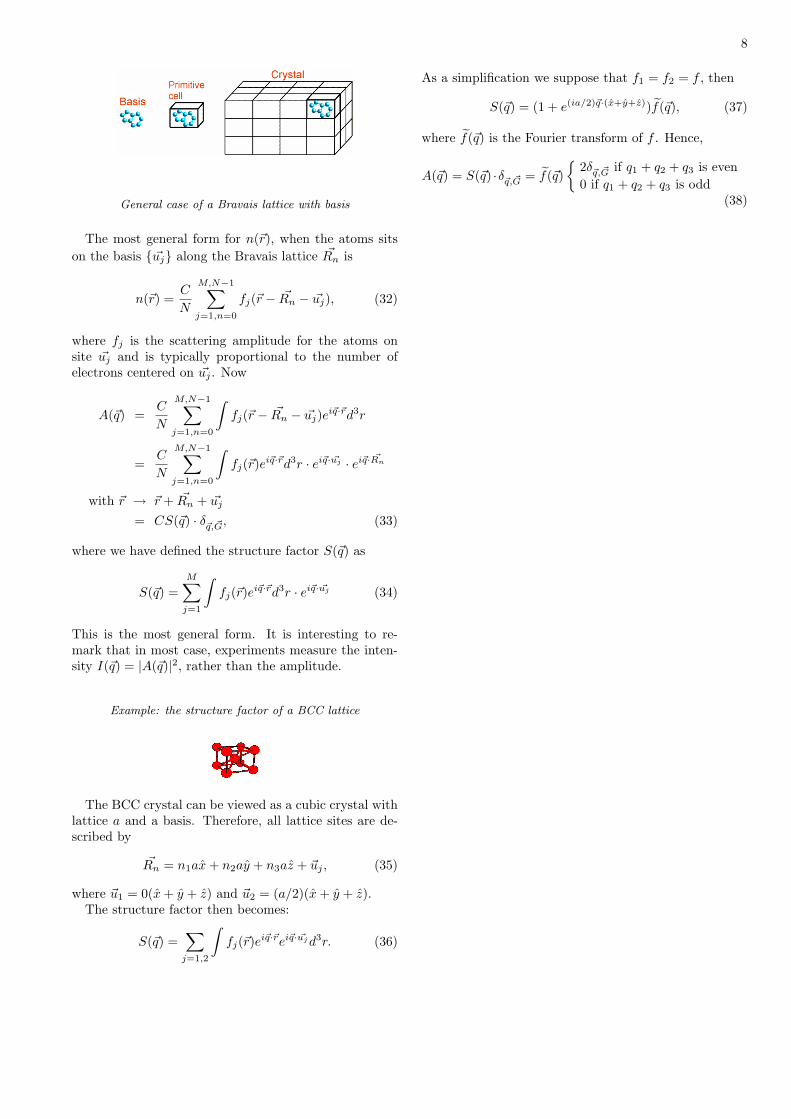
General case of a Bravais lattice with basis
The most general form for n(~r), when the atoms sitson the basis ~uj along the Bravais lattice ~Rn is
n(~r) =C
N
M,N−1∑
j=1,n=0
fj(~r − ~Rn − ~uj), (32)
where fj is the scattering amplitude for the atoms onsite ~uj and is typically proportional to the number ofelectrons centered on ~uj . Now
A(~q) =C
N
M,N−1∑
j=1,n=0
∫fj(~r − ~Rn − ~uj)ei~q·~rd3r
=C
N
M,N−1∑
j=1,n=0
∫fj(~r)ei~q·~rd3r · ei~q· ~uj · ei~q· ~Rn
with ~r → ~r + ~Rn + ~uj
= CS(~q) · δ~q, ~G, (33)
where we have defined the structure factor S(~q) as
S(~q) =M∑
j=1
∫fj(~r)ei~q·~rd3r · ei~q· ~uj (34)
This is the most general form. It is interesting to re-mark that in most case, experiments measure the inten-sity I(~q) = |A(~q)|2, rather than the amplitude.
Example: the structure factor of a BCC lattice
The BCC crystal can be viewed as a cubic crystal withlattice a and a basis. Therefore, all lattice sites are de-scribed by
~Rn = n1ax + n2ay + n3az + ~uj , (35)
where ~u1 = 0(x + y + z) and ~u2 = (a/2)(x + y + z).The structure factor then becomes:
S(~q) =∑
j=1,2
∫fj(~r)ei~q·~rei~q· ~uj d3r. (36)
As a simplification we suppose that f1 = f2 = f , then
S(~q) = (1 + e(ia/2)~q·(x+y+z))f(~q), (37)
where f(~q) is the Fourier transform of f . Hence,
A(~q) = S(~q) ·δ~q, ~G = f(~q)
2δ~q, ~G if q1 + q2 + q3 is even0 if q1 + q2 + q3 is odd
(38)
9
Bragg’s law
Equivalence between Bragg’s law for Miller planes andthe reciprocal lattice.
a
b
x
y
k1out
kin
q1=kin-k1out
q2=kin-k2out
θ
z
(1,0,0)
(0,1,0) Miller index
From Bragg’s law we know that for the planes perpen-dicular to x or Miller index (1,0,0) the following diffrac-tion condition applies:
nλ = 2a sin(θ). (39)
hence,
n2π
a= 2 sin(θ) · | ~kin| = |~q1|, (40)
since k = 2π/λ and we supposed that ~kin is perpendicularto z. This condition is equivalent to ~q1 = x2π/a ∈ ~G.The same relation applies for the scattering of the planeperpendicular to y or Miller index (0,1,0) the followingdiffraction condition applies:
nλ = 2b cos(θ). (41)
hence,
n2π
b= 2 cos(θ) · | ~kin| = |~q2|, (42)
or ~q2 = y2π/b ∈ ~G.
Summary of scattering
We have an incoming wave ei ~kin·~r diffracting on somesample with volume V and with a scattering probabilityn(~r) inside V . For X-ray n is typically given by the elec-tron distribution whereas for neutrons it is typically the
nuclear sites. The scattered wave amplitude with wavenumber ~k is then
A(~k − ~kin) ∼∫
V
d3rn(~r)ei(~k− ~kin)·~r (43)
This leads to three typical cases:
• Mono crystal diffraction: Point-like Braggpeaks
FIG. 8: Point-like Bragg peaks from a single crystal. (Ref:lassp.cornell.edu/lifshitz)
• Powder diffraction:
FIG. 9: Circle-like Bragg peaks from a powder with differentgrain sizes
• Liquid diffraction:
FIG. 10: Pattern evolution for a complex molecule evolvingfrom a crystal-like structure to an isotropic liquid
The liquid diffraction is essentially the limiting caseof the powder diffraction when the grain size be-comes comparable to the size of an atom.
10
PROPERTIES OF SOLIDS AND LIQUIDS
The Theory of everything discussed in the first sectioncan serve as a guideline to illustrate which part of theHamiltonian is important for a given property. For in-stance, when interested in the mechanical properties, theterms containing the electrons can be seen as a pertur-bation. However, when considering thermal conductivity,for example, the kinetic terms of the ions and the elec-trons are important.
In the following we will start by considering a few casesand we will start with the single electron approximation.
single electron approximation
The single electron approximation can be used to de-rive the energy and density of the electrons. This sim-plest model will always serve as a reference and in somecases the result is very close to the experimental value.Alkali metals (Li, Na, K,..) are reasonably well describedby this model, when we suppose that the outer shell elec-tron/atom (there is 1 for Li, Na, K) is free to move insidethe metal. This picture leads to the simple example of Nelectrons in a box. This box can be viewed as a uniformand positively charge background due to the atomic ions.We suppose that this box with size L×L×L has periodicboundary conditions, i.e.,
H = −N∑
n=1
~2∇2n
2mewith Ψ(0) = Ψ(L) (44)
For one electron the solutions can be written as
Ψ(~r) = ei~k·~r with E =~2|~k|22me
and ~k =2π
L(n1, n2, n3),
(45)where ni are the quantum numbers, which are positiveor negative integers. Since electrons are Fermions wecannot have two electrons in the same state, except forthe spin degeneracy. Hence each electron has to havedifferent quantum numbers. This implies that 2π/L isthe minimum difference between two electrons in k-space,which means that 1 electron uses up
(2π
L
)D
(46)
of volume in k-space, if D is the dimension of the space.If we now want to compute the electron density (numberof electrons per unit volume ne = N/LD) in the groundstate, which have k < kF (Fermi sphere with radius kF ),we obtain:
ne = 2 · V DkF·(
L
2π
)D
/LD, (47)
where the pre-factor 2 comes from the spin degeneracy.Hence,
n3De =
k3F
3π2in D = 3 since V D
kF=
4π
3k3
F (48)
n2De =
k2F
2πin D = 2 since V D
kF= πk2
F (49)
n1De =
2kF
πin D = 1 since V D
kF= 2kF , (50)
where the maximum energy of the electrons is
EF =~2k2
F
2methe Fermi energy (51)
This defines the Fermi energy: it is the highest energywhen all possible states with energy lower than EF areoccupied, which corresponds to the ground state of thesystem. This is one of the most important defi-nitions in condensed matter physics. The electrondensity can now be rewritten as a function of the Fermienergy, through eqs. (51) and (48) in 3D:
n(EF ) =(2mEF )3/2
3π2~3. (52)
We now want to define the energy density of statesD(E) as
n(EF ) ≡∫ EF
0
D(E)dE =⇒ D(E) =∂
∂En(E), (53)
which leads to
D(E) =m√
2mE
~3π2in 3D (54)
D(E) =m
~2πin 2D (55)
D(E) =
√2m
~2π2Ein 1D (56)
and illustrated below.
1D
2D
3D
D(E
)
E
FIG. 11: Density of states in 1D, 2D and 3D
Properties of the free electron model
Physical quantities at T=0:
11
• Average energy per electron: 〈E〉n = 3
5EF
• Pressure: P = −∂(〈E〉V )∂V = 2
5nEF , where 〈E〉V isthe total energy.
• Compressibility κ−1 = −V ∂P∂V = 2
3nEF
Case 2: T 6= 0: In equilibrium
fFD =1
e(E−µ)/kT + 1, (57)
where the chemical potential is the energy to add oneelectron µ = FN+1 − FN . µ = EF at T=0 and F is thefree energy.
The Sommerfeld expansion is valid for kT << µ and
〈H〉 =∫ ∞
0
dEH(E)FFD(E) (58)
'∫ µ
0
H(E)dE +π2
6(kT )2H ′(µ) + ... (59)
〈E〉 =∫ ∞
0
dEED(E)FFD(E) (60)
'∫ EF
0
ED(E)dE +π2
6(kT )2D(EF ) + ...(61)
〈n〉 = n(T = 0) (62)
⇒ µ(T ) ' EF − π2
6(kT )2
D′(EF )D(EF )
+ ... (63)
Physical quantities at T 6=0: Specific heat
CV =1V
∂〈E〉∂T
)
µ,V
=π2
3k2TD(EF ) (64)
Hence, CV
T = γ, which is the Sommerfeld parameter.
Periodic potentials
The periodicity of the underlying lattice has importantconsequences for many of the properties. We will walkthrough a few of them by starting with the simplest casein 1D.
Kronig-Penney model
Let us first consider the following simple periodic po-tential in 1D.
H = −~2∇2
2m− V
∑n
δ(x− na) (65)
The solutions for na < x < na+a are simply plane wavesand can be written as
ψ(x) = Aneikx + Bne−ikx. (66)
Now the task is to use the boundary conditions in orderto determine An and Bn. We have two conditions:
We now recall that the Eigenstate of the original Hamil-tonian is given by E(k) = ~2k2
2m , where eikx is the planewave between two δ functions, hence the dispersion re-lation is equal to E(k) = ~2k2
2m as long as −2 ≤ W ≤ 2.This condition will create gaps inside the spectrum asillustrated in the graph below:
0 1 2 3
∆EW<-
2
-2<W
<2
W<-2
E(k
)
π/a
FIG. 12: Dispersion curve for the Kronig-Penney model
Conclusion: a periodic potential creates gaps,which leads to the formation of a band structure.This is a very general statement which is true for almostany periodic potential.
Tight binging approximation
Let us consider the general potential due to the ar-rangement of the atoms on a lattice:
H = −~2∇2
2m+
∑n
V0(~r − ~Rn)
︸ ︷︷ ︸V (~r)
(78)
This is a very general form for a periodic potential assum-ing that we only have one type of atoms. The periodicityis given by the lattice index ~Rn. For a general periodicpotential Bloch’s theorem (see A& M for proof) tells usthat a solution to this Hamiltonian can be written as
ψk(~r) = ei~k·~ruk(~r), (79)
where uk is a periodic function such that uk(~r + ~Rn) =uk(~r). This implies that
ψk(~r + ~Rn) = ei~k· ~Rnψk(~r) (80)
Let us now suppose that the solution of the HamiltonianH1atom = −~2∇2
2m +V0(~r− ~Rn) with one atom is φl(~r− ~Rn)corresponding to the energy level εl, i.e., H1atomφl = εlφl.Now comes the important assumption, which allows usto simplify the problem: We suppose that
13
〈φl(r −Rm)|H|φl(r −Rn)〉 = −tl
∑
~i=x,y,z
δ~m,~n+~i + δ~m,~n−~i
+ εlδ~m,~n (81)
Hence, only the nearest neighbor in every direction istaken to be non-zero. Further, we assume that there is nooverlap between levels of the one atom potential, whichallows us to look for a general solution of the followingform for each energy level εl.
ψl(r) =∑
~n
cl~nφl(r −R~n) (82)
with eigenvalue El(k). To calculate El(k) we plug-inthis Ansatz into eq. (82) and obtain an equation forthe coefficients cl
~n, which leads to the following equationwhen using the tight binding approximation given in eq.(81).
cl~mεl − tl
∑
~i=±x,y,z
cl~m+~i
= El(k)cl~m (83)
The solution of this equation are plane waves, whichcan be verified readily by taking cl
~m = ei~k· ~Rm and plug-ging it into the equation to obtain
where ~a is the lattice constant in all 3 space directions:~a = R~m+a − R~m. The energy diagram is illustrated infig. . The degeneracy of each original single atomic en-ergy level εl is lifted by the coupling to the neighboringatoms and leads to a dispersion curve or electronic bandstructure.
-1.0 -0.5 0.0 0.5 1.0
ε3
ε2
−π/a k π/a
E
ε1
FIG. 13: Dispersion curve for the tight binding model
This tight binding approximation is very successfulin describing the electrons which are strongly bound tothe atoms. In the opposite limit where the electrons ormore plane-wave like, the weak potential approximationis more accurate:
Combining Bloch’s theorem with the tight bindingapproximation
The tight binding approximation is very general andcan be applied to almost any system, including non-periodic ones, where the tight binding elements can beassembled in an infinite matrix. For the periodic case,on the other hand, it is possible to describe the systemwith a finite matrix in order to obtain the full disper-sion relation. This is obtained by combining the Blochtheorem for periodic potentials, where the wave-functionfrom (79) is again:
ψk(~r) = ei~k·~ruk(~r)
Instead of writing (82) we write the Bloch-tight-binding solution as
ψkl (r) =
∑
~n
ei~k·R~ncl~nφl(r −R~n),
which now depends explicitly on the wavevector ~k. UsingBloch’s theorem this implies that
cl~n = cl
~m,
whenever ~n and ~m are related by a linear combination ofBravais vectors. Moreover, the tight binding equation in(83) is the same but with cl
~n replaced by cl~nei~k·R~n
A
B
a
FIG. 14: Diatomic square crystal
We apply this to the simple example of a diatomicsquare lattice of lattice constant a with alternating atomsA and B shown in figure . We will further assume thatwe have only one band l. Hence, the Bloch-tight-bindingsolution is written as
ψk(r) =∑
~n
ei~k·R~nc~nφ(r −R~n),
14
where c~n takes on only to possible values due to Bloch’stheorem: cA or cB . This leads to the following simplifiedtight binding equations (assuming 〈φl(r −Rn)|H|φl(r −Rn)〉 = εA or εB and t = −〈φl(r − Rn)|H|φl(r − Rm)〉when n and m are nearest neighbors):
cAεA − t∑
~i=±x,y cBeia~k·~i = E(~k)cA
cBεB − t∑
~i=±x,y cAeia~k·~i = E(~k)cB
It is now quite straightforward to rewrite these equa-tions in matrix form:
(εA −t · g
−t · g∗ εB
)(cA
cB
)= E(~k)
(cA
cB
),
with g = eia~k·x + e−ia~k·x + eia~k·y + e−ia~k·y. The disper-sion relation or band structure is then simply given byobtaining the eigenvalues of HBTB , where
HBTB =(
εA −t · g−t · g∗ εB
).
Weak potential approximation
In this case we consider the effect of the periodic po-tential V (~r) as a perturbation on the plane wave solution
ψ0k(~r) = ei~k·~r, with corresponding energies ε0k = ~2k2
2m andHamiltonian H0, i.e., H0ψ
0k(~r) = ε0kψ0
k(~r). Since the ori-gin of this energy dispersion relation can be chosen fromany site of the reciprocal lattice, we have ε0k+K = ε0k,hence these energies are degenerate. This implies thatwe have to use a degenerate perturbation theory. Themathematical procedure is very similar to the tight bind-ing approximation, but we now expand the solution ψ(~r)of the full Hamiltonian H = H0 +V (~r) in terms of a sumof plane waves ψ0
k(~r). Since ε0k+K = ε0k we will only usetwo plane waves in this expansion: ψ0
k(~r) and ψ0k+K(~r).
Hence,
ψ(~r) = αψ0k(~r) + βψ0
k+K(~r), (85)
where the coefficients α and β have to be determined inorder to solve Schrodinger’s equation:
(H − E)ψ(~r) = 0. (86)
We can find the solution by first multiplying (86) by(ψ0
k)∗(~r) and then integrating the equation over the wholespace which will lead to one equation, and we obtain asecond equation by multiplying (86) by (ψ0
k+K)∗(~r) andthen integrating of the whole space. This leads to
α
∫d3r(ψ0
k)∗(~r)(H − E)ψ0k(~r) + β
∫d3r(ψ0
k)∗(~r)(H − E)ψ0k+K(~r) = 0
α∫
d3r(ψ0k+K)∗(~r)(H − E)ψ0
k(~r) + β∫
d3r(ψ0k+K)∗(~r)(H − E)ψ0
k+K(~r) = 0 , (87)
where (assuming normalized plane waves in the integrals)
∫d3r(ψ0
k)∗(~r)(H − E)ψ0k(~r) =
∫d3re−ikr(H0 + V (r)− E)eikr = ε0k + 0− E∫
d3r(ψ0k)∗(~r)(H − E)ψ0
k+K(~r) =∫
d3re−ikr(H0 + V (r)− E)ei(k+K)r =∫
d3reiKr(ε0k+K + V (r)− E) = VK∫d3r(ψ0
k+K)∗(~r)(H − E)ψ0k+K(~r) = ε0k+K − E∫
d3r(ψ0k+K)∗(~r)(H − E)ψ0
k(~r) = V−K ,(88)
and V ~K =∫
d3rei ~K·~rV (~r) (the Fourier transform),∫
d3reiKr = 0 (for K 6= 0), and∫
d3rV (~r) = 0. With coefficients(88), equation (87) leads to the following couple of equations:
α(ε0k − E) + βVK = 0
αV−K + β(ε0k+K − E) = 0 ⇒∣∣∣∣ε0k − E VK
V−K ε0k+K − E
∣∣∣∣ = 0 ⇒ E = ε0k+ε0k+K
2 ±√
(ε0k−ε0k+K)2
4 + VKV−K . (89)
Finally if ε0k = ε0k+K , we have E = ε0k ± |VK |, whichleads to a splitting 2|VK | of the energy levels at thesedegenerate energies. For the example in figure , thisweak potential approximation would give us a splitting of2|VK=2π/a| at k = −π/a and k = K − π/a = π/a. Thisimplies that the first order calculation of the energy split-ting due to the weak periodic potential V (r) is equal totwice the fourier transform of this potential evaluated at
the wavevector which corresponds to the two dispersioncurves which led to the degenerate energy level.
Localization
When, instead of having a purely periodic potentialdisorder is included into the system, we no more have
15
Bloch wave solutions but localization of the wave func-tions occur. This is particularly important in low dimen-sional systems and tends to suppress transport.
Electronic properties due to periodic potential
Density of states
Density of states in 1D:
D(E) =∂n
∂E' δn
δE
=δn
δk
∣∣∣∣∂E(k)
∂k
∣∣∣∣−1
× 2︸︷︷︸spin
× 2︸︷︷︸∑±k
=1L
δN
δk
∣∣∣∣∂E(k)
∂k
∣∣∣∣−1
× 4
D(E) =2π
∣∣∣∣∂E(k)
∂k
∣∣∣∣−1
, (90)
where we used that δE = (∂E/∂k)δk and δk = 2π/L forone electron, i.e., δN = 1.
In three dimensions (D=3) we have:
D(E) =∂n
∂E' δn
δE
=∑
E(k)=E
δn
δk|∇kE(k)|−1 × 2︸︷︷︸
spin
=2
(2π)3
∫
E(k)=E
d2k |∇kE(k)|−1, (91)
where we used δE = (∇kE(k)) · δk,∑
E(k)=E(δk)2 →∫E(k)=E
d2k, and δn/(δk)3 = 1/(2π)3. This result showsthat the density of state in the presence of a periodicpotential, i.e., for a crystal depends only on the slope ofthe dispersion relation or the band structure.
Average velocity
The average velocity of an electron in a periodic po-tential is given by the expectation value of the velocity,i.e.,
〈v〉 = 〈ψ|v|ψ〉, (92)
where ψ is the wavefunction from the Hamiltonian withperiodic potential V , i.e., H = ~2∇2
2m + V . From Bloch’stheorem (79) we can write ψ(r) = eikruk(r), where uk(r)has the same periodicity as V (r). From the Schrodinger
equation Hψ = E(k)ψ it follows that uk is a solution of(~2
2m(k − i∇)2 + V − E(k)
)
︸ ︷︷ ︸Hk−E(k)
uk = 0. (93)
In order to calculate 〈v〉 we use first a first order pertur-bation in k + q, where q is very small. Therefore, theeigenvalue corresponding to Hk+q is E(k + q), which isto first order
Hence, the expectation value of the velocity is determinedby the slope of the dispersion relation. This also impliesthat the sign of the average velocity depends on the signof ∂E/∂k.
Response to an external field and existence of holes andelectrons
The idea is to describe the average motion of an elec-tron in the presence of an external field (electric, Eel, ormagnetic, B) in a semiclassical way. Hence, we want
m∗ d
dt〈v〉 = F = (qEel or q〈v〉 ×B), (95)
where m∗ is an affective mass and q the charge. Using(95) and (94) we have
m∗ ∂〈v〉∂k
k = qEel
1~m∗ ∂2E
∂k2k = qEel
⇒ ~k = qEel = F, (96)
Where we defined the effective mass m∗ as
m∗ = ~2
∣∣∣∣∂2E
∂k2
∣∣∣∣−1
. (97)
If ∂2E∂k2 is negative we need to change the sign of q in order
to remain consistent. Hence, when ∂2E∂k2 > 0, the charge
16
of an electron is q = −e but if ∂2E∂k2 < 0 then q is positive
(+e). In this case we describe the particles as holes.They represent missing electrons. With these definitionsof q and m∗, which is also called the band mass, thesemiclassical equations of motion of single electrons in aperiodic potential are simply given by eqs. (95) and (96).
In general, the effective mass is given by a tensor de-fined as
m∗αβ = ~2
∣∣∣∣∂2E
∂kα∂kβ
∣∣∣∣−1
, (98)
where α and β are the spatial directions. An importantconsequence of this semiclassical description of the mo-tion of electrons is the dependence of the effective masson the energy and the band structure. In some cases theeffective mass can even diverge (when ∂2E
∂k2 = 0). Sim-ilarly the sign of the carriers also depends on the bandstructure and the energy of the carriers. By definition wecall the bottom of an energy band and electronic bandwhen ∂2E
∂k2 > 0 and a hole band when at the top of theenergy band ∂2E
∂k2 < 0.
Bloch oscillations
In the presence of an electric field and a periodic po-tential we can use the equation of motion (96), i.e.,
~k = −eEel ⇒ k = −eEel
~t, (99)
but in a periodic potential and in the tight binding ap-proximation the energy is given by E(k) = −2t0 cos(ka),where a is the lattice constant and t0 the nearest neighboroverlap integral. Hence, since v = r and 〈v〉 = ~−1∂E/∂kwe have
〈r〉 =2t0eEel
cos(aeEelt
~). (100)
This means that the average position of the electronsoscillates in time (Bloch oscillations). In artificial struc-tures these Bloch oscillations are typically of the order of1THz.
Semiclassical motion in a magnetic field
In the presence of a magnetic field (B), we can describethe semiclassical trajectories in k-space using (96), i.e.,
~k = q〈v〉 ×B. (101)
Hence, only the values of k perpendicular to the magneticfield will change, which we denote by k⊥. The componentparallel to the field, k‖ is not affected by B. During asmall time difference
δt = t2 − t1 =∫ t2
t1
dt =∫ k2=k(t2)
k1=k(t1)
dk⊥/|k|. (102)
Using (101) and (94) and since k is perpendicular to 〈v〉and B, (k) ∼ ∂E/∂k‖ we obtain
δt =~2
qB
∫ k2
k1
dk⊥∂E/∂k‖
=~2
qB
d
dE
∫ k2
k1
k‖dk⊥. (103)
For a complete turn this leads to
T =~2
qB
d
dE
∮k‖dk⊥
︸ ︷︷ ︸S
. (104)
Here S is the area enclosed by an orbit in k-space. Thisorbit corresponds to an equipotential line perpendicularto the magnetic field.
Let’s suppose for simplicity that the effective mass ten-sor m∗ is diagonal and given by
m∗ =
mx 0 00 my 00 0 mz
(105)
and that the energy dispersion is harmonic (which is usu-ally true at a band extremum, i.e.,
E(k) =~2k2
x
2mx+~2k2
y
2my+~2k2
z
2mz. (106)
If we assume that the magnetic field is along z and thatthe average effective mass perpendicular to B is given bym⊥, we can rewrite (106) as
E(k) =~2k2
⊥2m⊥
+~2k2
‖2m‖
, (107)
where k2⊥ = k2
x+k2y. Using (104) and (107 we then obtain
S = πk2⊥ = π(2m⊥E/~2)− πk2
‖m⊥/m‖
⇒ dS
dE=
π2m⊥~2
⇒ ωc =2π
T=
qB
m⊥, (108)
which is the cyclotron frequency. Hence, the cyclotronfrequency depends on the average effective mass perpen-dicular to the magnetic field. This allows us to measurethe effective mass along different directions, simply bychanging the direction of the magnetic field and by mea-suring the cyclotron frequency.
Quantization of the cyclotron orbit: Landau levels
In quantum mechanics the energies of these cyclotronorbits become quantized. To see this we can write the
17
Hamiltonian of an electron in a magnetic field in the har-monic approximation (107) as
H =1
2m‖P 2‖ +
12m⊥
(P⊥ + qA)2, (109)
where B = ∇×A ⇒ A = −Byx in the Landau Gauge ifB is along z. In analogy to the harmonic oscillator, theeigenvalues of (109) are then given by
En,k‖ =~2k2
‖2m‖
+ (n + 1/2)~qB
m⊥︸︷︷︸ωc
. (110)
These eigenvalues can be found by writingthe wavefunction as ψ = eikxxφn(y − y0)eik‖z
with y0 = −~kx
qB , which leads to Hψ =(~2k2
‖2m‖
+ P 2y
2m⊥+ 1
2m⊥(
qBm⊥
)2
(y − y0)2)
φn(y − y0).
In the y direction this is simply the harmonic oscillatorwith eigenvalues (n + 1/2)~ωc and in the directionparallel to the field we have a plane wave so that thetotal energy is given by (110). The quantized levels(n + 1/2)~ωc due to the magnetic field are called theLandau levels.
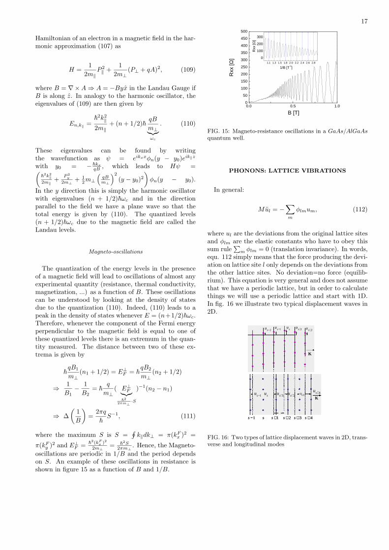
Magneto-oscillations
The quantization of the energy levels in the presenceof a magnetic field will lead to oscillations of almost anyexperimental quantity (resistance, thermal conductivity,magnetization, ...) as a function of B. These oscillationscan be understood by looking at the density of statesdue to the quantization (110). Indeed, (110) leads to apeak in the density of states whenever E = (n+1/2)~ωc.Therefore, whenever the component of the Fermi energyperpendicular to the magnetic field is equal to one ofthese quantized levels there is an extremum in the quan-tity measured. The distance between two of these ex-trema is given by
~qB1
m⊥(n1 + 1/2) = E⊥
F = ~qB2
m⊥(n2 + 1/2)
⇒ 1B1
− 1B2
= ~q
m⊥( E⊥
F︸︷︷︸~2
2πm⊥ ·S
)−1(n2 − n1)
⇒ ∆(
1B
)=
2πq
~S−1, (111)
where the maximum S is S =∮
k‖dk⊥ = π(kFx )2 =
π(kFy )2 and E⊥
F = ~2(kFx )2
2m⊥= ~2S
2πm⊥. Hence, the Magneto-
oscillations are periodic in 1/B and the period dependson S. An example of these oscillations in resistance isshown in figure 15 as a function of B and 1/B.
0.0 0.5 1.00
50
100
150
200
250
300
350
400
450
500
1.1 1.3 1.5 1.8 2.0 2.2 2.4 2.6 2.8
0
100
200
300
Rxx
[Ω]
B [T]
Rxx
[Ω]
1/B [T-1]
FIG. 15: Magneto-resistance oscillations in a GaAs/AlGaAsquantum well.
PHONONS: LATTICE VIBRATIONS
In general:
Mul = −∑m
φlmum, (112)
where ul are the deviations from the original lattice sitesand φlm are the elastic constants who have to obey thissum rule
∑m φlm = 0 (translation invariance). In words,
equ. 112 simply means that the force producing the devi-ation on lattice site l only depends on the deviations fromthe other lattice sites. No deviation=no force (equilib-rium). This equation is very general and does not assumethat we have a periodic lattice, but in order to calculatethings we will use a periodic lattice and start with 1D.In fig. 16 we illustrate two typical displacement waves in2D.
1−su su 1+su 2+su 3+su 4+su
K
1−s s 1+s 2+s 3+s 4+s
1−su su 1+su 2+su 3+su 4+su
K
1−s s 1+s 2+s 3+s 4+s
2−su 1−su su 1+su2+su
K
2−su 1−su su 1+su2+su
K
FIG. 16: Two types of lattice displacement waves in 2D, trans-verse and longitudinal modes
18
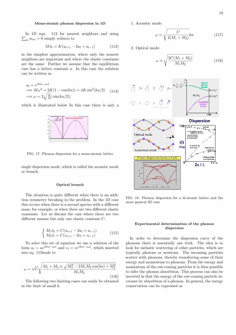
Mono-atomic phonon dispersion in 1D
In 1D equ. 112 for nearest neighbors and using∑m φlm = 0 simply reduces to
Mul = K(ul+1 − 2ul + ul−1) (113)
in the simplest approximation, where only the nearestneighbors are important and where the elastic constantsare the same. Further we assume that the equilibriumcase has a lattice constant a. In this case the solutioncan be written as
ul = eikla−iωt
=⇒ Mω2 = 2K(1− cos(ka)) = 4K sin2(ka/2)
=⇒ ω = 2√
KM | sin(ka/2)|
(114)
which is illustrated below In this case there is only a
0 -π/a π/a 2π/a
0
0.2
0.4
0.6
0.8
1.0
1.2
k
( )MK2
ω Mono-atomic dispersion
FIG. 17: Phonon dispersion for a mono-atomic lattice
single dispersion mode, which is called the acoustic modeor branch.
Optical branch
The situation is quite different when there is an addi-tion symmetry breaking in the problem. In the 1D casethis occurs when there is a second species with a differentmass, for example, or when there are two different elasticconstants. Let us discuss the case where there are twodifferent masses but only one elastic constant C:
To solve this set of equation we use a solution of theform ul = ueikla−iωt and vl = veikla−iωt, which insertedinto eq. 115leads to
ω =√
C
√M1 + M2 ±
√M2
1 − 2M1M2 cos(ka) + M22
M1M2
(116)The following two limiting cases can easily be obtained
in the limit of small k.
1. Acoustic mode:
ω '√
C
2(M1 + M2)ka (117)
2. Optical mode:
ω '√
2C(M1 + M2)M1M2
(118)
FIG. 18: Phonon dispersion for a di-atomic lattice and themore general 3D case
Experimental determination of the phonondispersion
In order to determine the dispersion curve of thephonons there is essentially one trick. The idea is tolook for inelastic scattering of other particles, which aretypically photons or neutrons. The incoming particlesscatter with phonons, thereby transferring some of theirenergy and momentum to phonons. From the energy andmomentum of the out-coming particles it is then possibleto infer the phonon absorbtion. This process can also beinverted in that the energy of the out-coming particle in-creases by absorbtion of a phonon. In general, the energyconservation can be expressed as
19
~ωin(~k)− ~ω′out(~k′)︸ ︷︷ ︸in/out particle
= ±~Ω( ~K)︸ ︷︷ ︸phonon
(119)
and the momentum conservation as
~~k − ~~k′ = ±~ ~K + ~~G, (120)
where ~G is a reciprocal lattice vector. A neutron scat-tering experiment is illustrated below.
FIG. 19: Inelastic neutron scattering experiment in ChalkRiver used to determine the phonon dispersion
Origin of the elastic constant
From the TOE we have the potential term due to theinteractions between ions.
Hions = −Nions∑
i
~2∇2i
2mi+
Nions∑
i<j
qiqj
|ri − rj | (121)
This leads to a potential of the form
φ(r1, . . . , rn) = φ(r01, . . . , r
0n)︸ ︷︷ ︸
Cohesive energyEquilibrium pos.
+∑
i
∂φ
∂ri
)
r0i
displacment︷︸︸︷ui
︸ ︷︷ ︸0
+12
∑
i,j
∂2φ
∂ri∂rj
r0i︸ ︷︷ ︸
φi,j
uiuj + · · · (122)
The linear term has to be zero for stability reasons (nominimum in energy otherwise). The classical equationof motion is then simply given by equ. 112, because~F = −~∇φ. To solve this equation in general, one canwrite a solution of the form
~ul = ~ε · ei~k· ~Rl−iωt, (123)
where ~Rl are the lattice sites. One then has to solvefor the dispersion relation ω(~k) in all directions, as illus-
trated in fig. 18. From 123 we have
mω2~ε =∑m
φl,mei~k·( ~Rl− ~Rm)
︸ ︷︷ ︸φ(k)
·~ε (124)
,where φ(k) is a 3× 3 matrix, since φlm too. This leads
to an eigenvalue equation for ω2 with three eigenvalues:ω2
L (for ~k ‖ ~ε) and ω2T (1,2) (for ~k ⊥ ~ε). Hence, we have
on longitudinal mode and two transverse modes and allphonon modes can be described by a superposition ofthese.
If we have two different masses, we have two addi-
20
tional equations of the form (124). This leads to thegeneral case, where one has two branches the optical oneand the acoustic one and each is divided in longitudinaland transverse modes. The acoustic branch has alwaysa dispersion going to zero at k = 0, whereas for the op-tical mode at k = 0 the energy is non-zero. The acous-tic phonons have a gapless excitation spectrum and cantherefore be created at very low energy as opposed tooptical phonons which require a miniumum energy to beexcited.
Quantum case
While many of the properties, like the dispersion rela-tion, can be explained in classical terms, which are simplyvibrations of the crystal ions, others, such as statisticalproperties need a quantum mechanical treatment.
Phonons can simply be seen as harmonic oscillatorswhich carry no spin (or spin 0). They can, therefore, beaccurately described by bosons with energy
En(k) = ~ω(k)(n + 1/2). (125)
We can now calculate the density of states of phonons,or the number of states between ω and ω + dω, i.e.,
D(ω)dω =1
(2π)3
∫ ω+dω
ω
dk (126)
but dω = ∇kωdk, hence
D(ω) =1
(2π)3
∫
ω=const
dSω
|∇kω| (127)
Let us now suppose that we have 3 low energy modeswith linear dispersion, one longitudinal mode ωL(k) =cLk and two transverse modes ωT (k) = cT k, hence∇ωL,T (k) = cL,T , which implies that
∫dS = 4πk2. This
leads to a density of state
DL,T (ω) =k2
2π2cL,T=
ω2
2π2c3L,T
(128)
or
Dtot(ω) =ω2
2π2
(1c3L
+2c3T
)
︸ ︷︷ ︸1
c3
(129)
in the isotropic case.From statistics we know that the probability to find a
state at E = En is given by the Boltzmann distributionPn ∼ e−En/kBT , with normalization
∑Pn = 1. Hence,
Pn = e−n~ω/kBT (1− e−~ω/kBT ) (130)
simply from the normalization condition. We can nowcalculate the average energy at ω,
E(ω) =∑
n
EnPn = (1− e−~ω/kBT )~ω∞∑
n=0
(n + 1/2)(e−~ω/kBT )n
= ~ω
12
+1
e~ω/kBT − 1︸ ︷︷ ︸〈n〉
(131)
here 〈n〉 is the expectation value of quantum number nat T , which is nothing else but the Bose Einstein distri-bution. As is well known, Bosons obey the Bose-Einsteinstatistics, where he Bose-Einstein distribution function isgiven by
fBE =1
eE/kBT − 1(132)
Important: at T = 0, fBE is simply a delta functionδ(E). This is the Bose-Einstein condensation, where the
zero energy state is totally degenerate (this does sup-pose that there are no interactions between bosons, withinteractions the delta function will be a little broader).The total average energy can then be calculated from thedensity of states as:
〈E〉 =∫
dωD(ω)E(ω) (133)
This also allows us to calculate the specific heat CV =
21
ddT 〈E〉 in the isotropic case and in the linear dispersionapproximation D(ω) ∼ ω2/c3, hence
CV =d
dT
∫ ∞
0
dωD(ω)E(ω)
=d
dT
∫ ∞
0
dωD(ω)~ω
e~ω/kBT − 1
=d
dT
32π2
1c3︸︷︷︸
13
(1
c3L
+ 2c3T
)
∫ ∞
0
dω~ω3
e~ω/kBT − 1︸ ︷︷ ︸∫∞0 dω x3
ex−1(kBT )4
~3
=d
dT
3(kBT )4
2π2(c~)3
∫ ∞
0
dωx3
ex − 1︸ ︷︷ ︸π4/15
=2π2kB
5
(kBT
~c
)3
(134)
where we had defined the variable x = ~ω/kBT andwhere 1/c3 is the average over the 3 acoustic modes.
The Debye model assumes a linear dispersion (ω = ck)and uses the analogy to electrons where (n = k3
F /3π2) todefine kD. Since phonons have no spins one obtains:
n =k3
D
6π2and
kBΘD = ~ωD = ~ckD (ΘD: Debye temperature)
=⇒ CV =12π4kB
5
(T
ΘD
)3
· n (135)
The typical Debye temperature is of the order of 100K.Finally, combining this result with the contributions fromelectrons (64), we obtain the expression valid for low tem-peratures:
CV = γT︸︷︷︸electrons
+ βT 3
︸︷︷︸phonons
(136)
TRANSPORT (BOLTZMANN THEORY)
Transport allows us to calculate transport coefficientssuch as resistances and thermal conductivities. Whileseveral transport theories exist, Boltzmann’s approachis the most powerful and applies to most situations incondensed matter. The main idea in Boltzmann theoryis to describe the electrons by a distribution function g.In equilibrium g is simply the Fermi-Dirac distributionfunction fFD. In general, g(r, k, t) and at t−dt it can bewritten as:
g(r − rdt, k − kdt, t− dt) (137)
If the electrons flow without collisions,(137)=g(r, k, t) = fFD. The situation changes ifcollisions (f. ex. between electrons, impurities, orphonons) are included. In this case
where gcoll. describes the collisions. gcoll. = 0 withoutcollisions. Expanding (137) to first order and using (138)we obtain
r∂g
∂r+ k
∂g
∂k+
∂g
∂t︸ ︷︷ ︸dgdt
=dg
dt
)
coll.
(139)
This is Boltzmann’s equation.
Relaxation time approximation
Solving Boltzmann’s equation is not easy in generaland therefore approximations are used. The simplest oneis the relaxation time (τ) approximation. In this approx-imation:
dg
dt
)
coll.
= −1τ
(g − fFD)
=⇒ dg
dt= −1
τ(g − fFD) (140)
It is quite intuitive to see from where this approxima-tion comes from, since a kick at t = 0 would lead tosolution of the form
g(t) =e−t/τ
τ+ fFD → fFD (when t = ∞) (141)
This is the basic framework, which allows us to eval-uate the effect of external fields on the system and toestimate the linear response to them.
Case 1: ~F = −e ~E
In this case we look for a response in current densityand define the conductivity tensor in linear response as
~j = σ ~E
⇒ jα = σαβEβ = −2e
∫d3k
(2π)3vαg(r, k, t). (142)
Since we are interested in the case of a homogenousuniform electric field, ∂g/∂t = 0 and ∂g/∂r = 0 and
22
~k = −eE, Boltzmann’s equation (139) in the relaxationtime approximation becomes
k∂g
∂k︸︷︷︸−e ~E~
∂g∂ε · ∂ε
∂~k
= −1τ
(g − fFD)
⇒ g =e ~Eτ
~∂g
∂ε︸︷︷︸'− ∂fF D
∂µ
· ∂ε
∂~k︸︷︷︸~~v
+fFD (143)
Here we used the first order approximation ∂g/∂ε '−∂fFD/∂µ, which is justified if the correction g−fFD issmoother than ∂fFD/∂µ, which is close to a delta func-tion when kT << EF . Hence, using (143) to evaluatethe current (142), we obtain
jα = 2e
∫d3k
(2π)3vαeτ ~E · ~v ∂fFD
∂µ+ ∼ (
∫vαfFD)
︸ ︷︷ ︸=0
, (144)
which leads to
σαβ =∂jα
∂Eβ= 2e2
∫d3k
(2π)3vαvβ
∂fFD
∂µτ(ε) (145)
This is one of the most important expressions for theconductivity. Since ∂fFD/∂µ is almost a delta functionfor kT << EF this expression shows that only electronsclose to the chemical potential µ will significantly con-tribute to transport. It is possible to evaluate (145) insimple cases.
Let’s assume that τ does not depend on the energy,then we can rewrite (145) as
σαβ = 2e2τ
∫d3k
(2π)3vα
∂ε
~∂kβ
(−∂fFD
∂ε
)
= e2τ
∫d3k
(2π)3vα
(−∂fFD
~∂kβ
)
= e2τ
∫d3k
(2π)3∂vα
∂kβ︸︷︷︸~δαβ/m∗
fFD/~−∫
k⊥β
fFDvα
︸ ︷︷ ︸=0
=e2τ
m∗
∫2
d3k
(2π)3fFD
︸ ︷︷ ︸n
δαβ (146)
• If τ(ε) = τ we therefore obtain the most importantformula of conductivity (the Drude formula)
σαβ =e2τn
m∗ δαβ (147)
Using the same approach but in the presence of a mag-netic field, ~F = −e ~E−e~v× ~B, we can derive an equivalentexpression for σαβ , but in this case the off-diagonal com-ponent is not zero anymore. (See assignment).
Diffusion model of transport (Drude)
In the case where the scattering of electrons is domi-nated by inelastic diffusion, we can write a very simpleform for the conductivity or resistivity tensor. Indeed, ina diffusive regime the average velocity is directly propor-tional to the external force and to the inverse effectivemass. The proportionality coefficient is then simply thescattering probability 1/τ . Hence,
m∗
τ~v = ~F = −e ~E − e~v × ~B (148)
If we suppose that the magnetic field is small and inthe z direction and ~E along x, then eq. (148) becomes
e ~E︸︷︷︸eEx
= −m∗
τ~v
︸ ︷︷ ︸'m∗jx
τen
−e~v × ~B︸ ︷︷ ︸'jyB/n
Ex =m∗
ne2τjx +
B
nejy (149)
Since in general ~E = ρ~j and because the resistivityalong ~B is not affected by the magnetic field we can writefor ~B in the z direction,
ρ =
m∗ne2τ
Bne 0
− Bne
m∗ne2τ 0
0 0 m∗ne2τ
= σ−1 (150)
This is the famous Drude formula in a magnetic field.This formula is in fact equivalent to the relaxation timeapproximation in the Boltzmann theory (147).
Case 2: Thermal inequilibrium
We now consider the case, where we also have a spacialgradient. Hence (139) and (140) become
r∂g
∂r︸︷︷︸'~v· ∂f
∂~r
+ k∂g
∂k︸︷︷︸'−e ~E·~v ∂f
∂ε
= −1τ
(g − fFD), (151)
here we used again that g − f is smooth so that ∂(g −f)/∂ε << ∂f/∂ε. Moreover, since
fFD =1
e(ε−µ(r))/kT (r) + 1
⇒ ∂f
∂r=
∂f
∂ε
(−∇rµ− (ε− µ)
∇rT
T
)
⇒ g = ~v · ∂f
∂ετ
(e ~G + (ε− µ)
∇rT
T
)+ fFD,(152)
23
where we defined the generalized field e ~G = e ~E+~∇µ(r)and the external forces are now −e ~E, ~∇µ(r) and ~∇T (r),corresponding to an external electrical field, a gradientin the chemical potential (f.ex. a density gradient), anda temperature gradient. The electrical current density isthe same as before but is now expressed (in the linearresponse) in terms of the additional external fields:
~je = −2e
∫d3k
(2π)3~vg ' L11 ~G + L12
(−~∇T
T
). (153)
An expression for the thermal current can be de-duced from the following thermodynamical relation dQ =TdS = dU − µdN , hence
~jQ = 2e
∫d3k
(2π)3(ε− µ)~vg ' L21 ~G + L22
(−~∇T
T
).
(154)Here Lαβ are the linear transport coefficients and σ =
L11. We now want to evaluate these expressions in thelow temperature limit, where we can use ∂fFD/∂µ 'δ(ε − εF ), hence the expression for σ in (145) can bewritten as
σαβ(x) =∂jα
∂Eβ= 2e2
∫d3k
(2π)3vαvβτ(x)δ(ε− x), (155)
where σαβ = σαβ(εF ). We will use this new function σ(x)to express the other transport coefficients. For instancein linear response,
e2L22αβ =
∂jQ
∂(−~∇T
T
)β
= 2e2
∫d3k
(2π)3vαvβ(ε− µ)2τ(ε)
∂f
∂µ
=∫
dx∂f
∂µ(ε− µ)2σαβ(ε). (156)
Using that (εF − µ) ' π2
6 (kT )2D′(εF )/D(εF ), we ob-tain (derivation in assignment).
L22αβ =
π2
3e2(kT )2σαβ(εF ) and similarly
L12αβ = L21
αβ = −π2
3e(kT )2σ′αβ(εF )
L11αβ = σαβ(εF ) (157)
Physical quantities
• Thermal conductivity (κ): jQ = κ(−∇T )
Is obtained from eqs. (153,154,157), by setting je =0, hence at low temperatures, L11 ~G+L12
(− ~∇T
T
)=
0 and
jQ = (L12(L11)−1L12
︸ ︷︷ ︸∼O(T 4)'0
−L22)
(−
~∇T
T
)
= −L22
T∇T
⇒ καβ =π2
3k2T
e2σαβ (158)
This is the well known Wiedemann-Franz law
• Thermopower (Q): ~E = Q∇T with je = 0. Inthis case
Historical note:The Seebeck effect: The discovery of thermoelectricity
dates back to Seebeck [1] (1770-1831). Thomas Johann See-beck was born in Revel (now Tallinn), the capital of Estoniawhich at that time was part of East Prussia. Seebeck was amember of a prominent merchant family with ancestral rootsin Sweden. He studied medicine in Germany and qualifiedas a doctor in 1802. Seebeck spent most of his life involvedin scientific research. In 1821 he discovered that a compassneedle deflected when placed in the vicinity of a closed loopformed from two dissimilar metal conductors if the junctionswere maintained at different temperatures. He also observedthat the magnitude of the deflection was proportional to thetemperature difference and depended on the type of conduct-ing material, and does not depend on the temperature distri-bution along the conductors. Seebeck tested a wide range ofmaterials, including the naturally found semiconductors ZnSband PbS. It is interesting to note that if these materials hadbeen used at that time to construct a thermoelectric genera-tor, it could have had an efficiency of around 3% - similar tothat of contemporary steam engines.
The Seebeck coefficient is defined as the open circuit volt-age produced between two points on a conductor, where auniform temperature difference of 1K exists between thosepoints.
The Peltier effect: It was later in 1834 that Peltier[2] de-scribed thermal effects at the junctions of dissimilar conduc-tors when an electrical current flows between the materials.Peltier failed however to understand the full implications ofhis findings and it wasn’t until four years later that Lenz[3]concluded that there is heat adsorption or generation at thejunctions depending on the direction of current flow.
The Thomson effect: In 1851, Thomson[4] (later LordKelvin) predicted and subsequently observed experimentallythe cooling or heating of a homogeneous conductor resultingfrom the flow of an electrical current in the presence of atemperature gradient. This is know as the Thomson effectand is defined as the rate of heat generated or absorbed in a
24
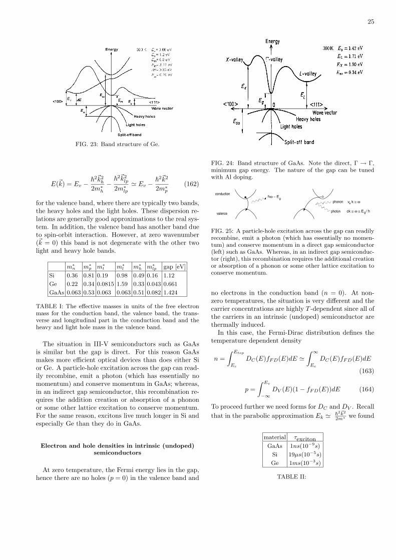
FIG. 20: Thermoelectric cooling (left): If an electric currentis applied to the thermocouple as shown, heat is pumped fromthe cold junction to the hot junction. The cold junction willrapidly drop below ambient temperature provided heat is re-moved from the hot side. The temperature gradient will varyaccording to the magnitude of current applied. Thermoelec-tric generation (right): The simplest thermoelectric generatorconsists of a thermocouple, comprising a p-type and n-typethermoelement connected electrically in series and thermallyin parallel. Heat is pumped into one side of the couple andrejected from the opposite side. An electrical current is pro-duced, proportional to the temperature gradient between thehot and cold junctions.
single current carrying conductor subjected to a temperaturegradient.
[1] Seebeck, T.J., 1822, Magnetische Polarisation der Met-alle und Erzedurch Temperatur-Differenz. Abhand Deut.Akad. Wiss. Berlin, 265-373.
[2] Peltier, J.C., 1834, Nouvelles experiences sur la calo-riecete des courans electriques. Ann. Chem., LVI, 371-387.
[4] Thomson, W., 1851, On a mechanical theory of thermo-electric currents, Proc.Roy.Soc.Edinburgh, 91-98.
SEMICONDUCTORS
Semiconductors are distinguished from metals in thatthey have a gap at the Fermi surface, and are distin-guished from insulators in that the gap is smaller, whichis ambiguous. But generally, if the gap is close to 1eVit’s a standard semiconductor. If the gap is close to 3eVit’s a wide band gap semiconductor and above 6eV it’susually called an insulator. Typically, the distinction issimply made from the temperature dependence of theconductivity. If σ → 0 for T → 0 it’s a semiconductor oran insulator but the material is a metal if σ → σ0 > 0.However, even at room temperatures the conductivitiesof pure materials differ by many orders of magnitude(σmetal >> σsemi >> σinsu).
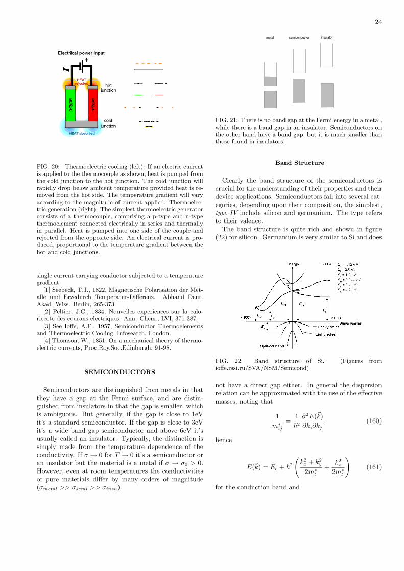
metal insulatorsemiconductor
FIG. 21: There is no band gap at the Fermi energy in a metal,while there is a band gap in an insulator. Semiconductors onthe other hand have a band gap, but it is much smaller thanthose found in insulators.
Band Structure
Clearly the band structure of the semiconductors iscrucial for the understanding of their properties and theirdevice applications. Semiconductors fall into several cat-egories, depending upon their composition, the simplest,type IV include silicon and germanium. The type refersto their valence.
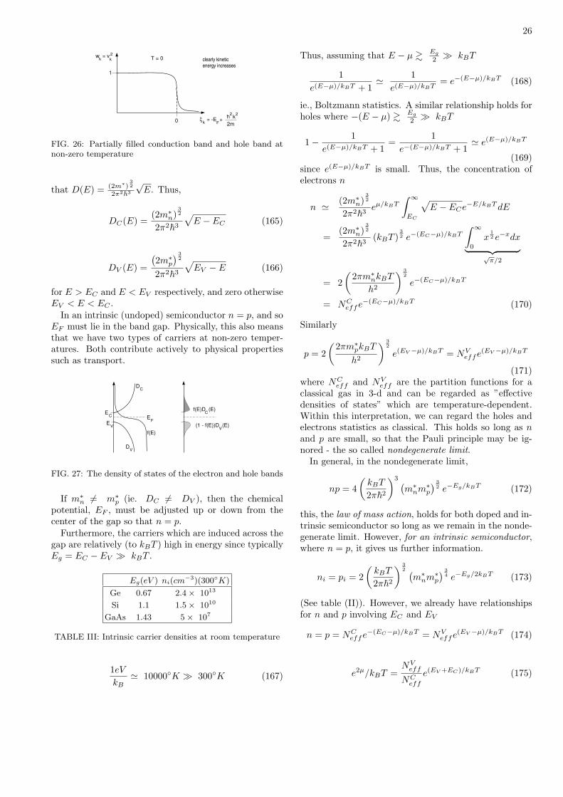
The band structure is quite rich and shown in figure(22) for silicon. Germanium is very similar to Si and does
FIG. 22: Band structure of Si. (Figures fromioffe.rssi.ru/SVA/NSM/Semicond)
not have a direct gap either. In general the dispersionrelation can be approximated with the use of the effectivemasses, noting that
1m∗
ij
=1~2
∂2E(~k)∂ki∂kj
, (160)
hence
E(~k) = Ec + ~2
(k2
x + k2y
2m∗t
+k2
x
2m∗l
)(161)
for the conduction band and
25
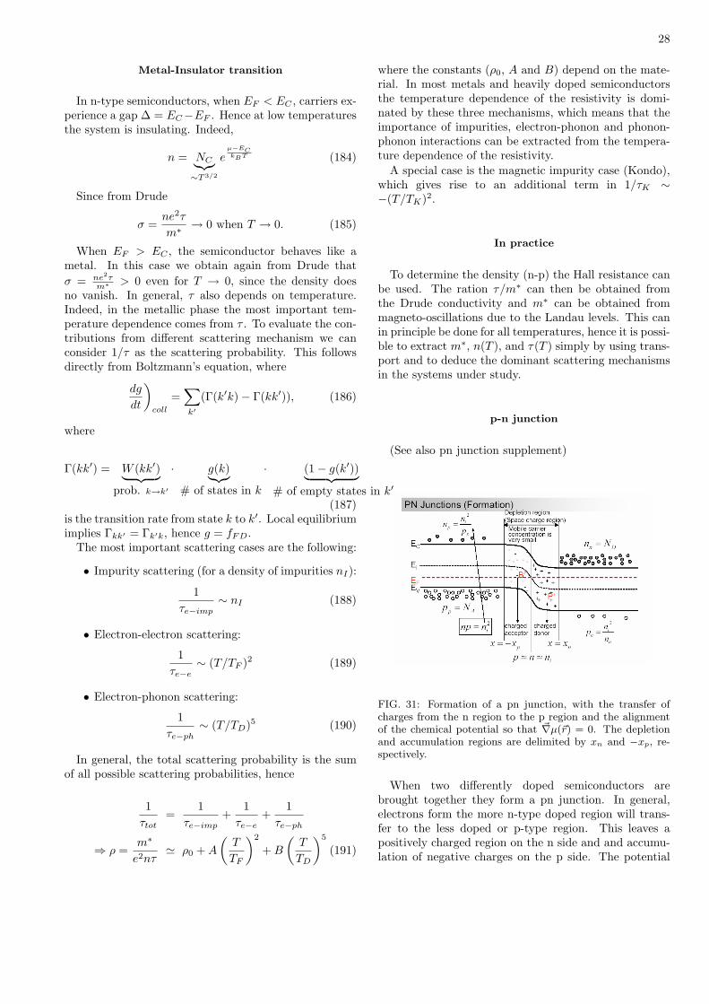
FIG. 23: Band structure of Ge.
E(~k) = Ev − ~2~k2
h
2m∗h
− ~2~k2
lp
2m∗lp
' Ev − ~2~k2
2m∗p
(162)
for the valence band, where there are typically two bands,the heavy holes and the light holes. These dispersion re-lations are generally good approximations to the real sys-tem. In addition, the valence band has another band dueto spin-orbit interaction. However, at zero wavenumber(~k = 0) this band is not degenerate with the other twolight and heavy hole bands.
m∗n m∗
p m∗t m∗
l m∗h m∗
lp gap [eV]
Si 0.36 0.81 0.19 0.98 0.49 0.16 1.12
Ge 0.22 0.34 0.0815 1.59 0.33 0.043 0.661
GaAs 0.063 0.53 0.063 0.063 0.51 0.082 1.424
TABLE I: The effective masses in units of the free electronmass for the conduction band, the valence band, the trans-verse and longitudinal part in the conduction band and theheavy and light hole mass in the valence band.
The situation in III-V semiconductors such as GaAsis similar but the gap is direct. For this reason GaAsmakes more efficient optical devices than does either Sior Ge. A particle-hole excitation across the gap can read-ily recombine, emit a photon (which has essentially nomomentum) and conserve momentum in GaAs; whereas,in an indirect gap semiconductor, this recombination re-quires the addition creation or absorption of a phononor some other lattice excitation to conserve momentum.For the same reason, excitons live much longer in Si andespecially Ge than they do in GaAs.
Electron and hole densities in intrinsic (undoped)semiconductors
At zero temperature, the Fermi energy lies in the gap,hence there are no holes (p = 0) in the valence band and
FIG. 24: Band structure of GaAs. Note the direct, Γ → Γ,minimum gap energy. The nature of the gap can be tunedwith Al doping.
conduction
valence
hω ∼ Eg
phonon
photon
v k ≅ ωs
ck ≅ ω ≅ E / hg
FIG. 25: A particle-hole excitation across the gap can readilyrecombine, emit a photon (which has essentially no momen-tum) and conserve momentum in a direct gap semiconductor(left) such as GaAs. Whereas, in an indirect gap semiconduc-tor (right), this recombination requires the additional creationor absorption of a phonon or some other lattice excitation toconserve momentum.
no electrons in the conduction band (n = 0). At non-zero temperatures, the situation is very different and thecarrier concentrations are highly T -dependent since all ofthe carriers in an intrinsic (undoped) semiconductor arethermally induced.
In this case, the Fermi-Dirac distribution defines thetemperature dependent density
n =∫ Etop
Ec
DC(E)fFD(E)dE '∫ ∞
Ec
DC(E)fFD(E)dE
(163)
p =∫ Ev
−∞DV (E)(1− fFD(E))dE (164)
To proceed further we need forms for DC and DV . Recallthat in the parabolic approximation Ek ' ~2~k2
2m∗ we found
material τexcitonGaAs 1ns(10−9s)
Si 19µs(10−5s)
Ge 1ms(10−3s)
TABLE II:
26
0
w = v k k
2
T = 0
k Fξ = -E +
h k2 2
2m
clearly kinetic energy increases
1
FIG. 26: Partially filled conduction band and hole band atnon-zero temperature
that D(E) = (2m∗)32
2π2~3√
E. Thus,
DC(E) =(2m∗
n)32
2π2~3
√E − EC (165)
DV (E) =
(2m∗
p
) 32
2π2~3
√EV − E (166)
for E > EC and E < EV respectively, and zero otherwiseEV < E < EC .
In an intrinsic (undoped) semiconductor n = p, and soEF must lie in the band gap. Physically, this also meansthat we have two types of carriers at non-zero temper-atures. Both contribute actively to physical propertiessuch as transport.
EF
EC
EV
VD
f(E)
DC
Cf(E)D (E)
V(1 - f(E))D (E)
FIG. 27: The density of states of the electron and hole bands
If m∗n 6= m∗
p (ie. DC 6= DV ), then the chemicalpotential, EF , must be adjusted up or down from thecenter of the gap so that n = p.
Furthermore, the carriers which are induced across thegap are relatively (to kBT ) high in energy since typicallyEg = EC − EV À kBT .
Eg(eV ) ni(cm−3)(300K)
Ge 0.67 2.4× 10¹³
Si 1.1 1.5× 10¹⁰
GaAs 1.43 5× 10⁷
TABLE III: Intrinsic carrier densities at room temperature
1eV
kB' 10000K À 300K (167)
Thus, assuming that E − µ & Eg
2 À kBT
1e(E−µ)/kBT + 1
' 1e(E−µ)/kBT
= e−(E−µ)/kBT (168)
ie., Boltzmann statistics. A similar relationship holds forholes where −(E − µ) & Eg
2 À kBT
1− 1e(E−µ)/kBT + 1
=1
e−(E−µ)/kBT + 1' e(E−µ)/kBT
(169)since e(E−µ)/kBT is small. Thus, the concentration ofelectrons n
n ' (2m∗n)
32
2π2~3eµ/kBT
∫ ∞
EC
√E − ECe−E/kBT dE
=(2m∗
n)32
2π2~3(kBT )
32 e−(EC−µ)/kBT
∫ ∞
0
x12 e−xdx
︸ ︷︷ ︸√π/2
= 2(
2πm∗nkBT
h2
) 32
e−(EC−µ)/kBT
= NCeffe−(EC−µ)/kBT (170)
Similarly
p = 2(
2πm∗pkBT
h2
) 32
e(EV −µ)/kBT = NVeffe(EV −µ)/kBT
(171)where NC
eff and NVeff are the partition functions for a
classical gas in 3-d and can be regarded as ”effectivedensities of states” which are temperature-dependent.Within this interpretation, we can regard the holes andelectrons statistics as classical. This holds so long as nand p are small, so that the Pauli principle may be ig-nored - the so called nondegenerate limit.
In general, in the nondegenerate limit,
np = 4(
kBT
2π~2
)3 (m∗
nm∗p
) 32 e−Eg/kBT (172)
this, the law of mass action, holds for both doped and in-trinsic semiconductor so long as we remain in the nonde-generate limit. However, for an intrinsic semiconductor,where n = p, it gives us further information.
ni = pi = 2(
kBT
2π~2
) 32 (
m∗nm∗
p
) 34 e−Eg/2kBT (173)
(See table (II)). However, we already have relationshipsfor n and p involving EC and EV
n = p = NCeffe−(EC−µ)/kBT = NV
effe(EV −µ)/kBT (174)
e2µ/kBT =NV
eff
NCeff
e(EV +EC)/kBT (175)
27
or
µ =12(EV + EC) +
12kBT ln
(NV
eff
NCeff
)(176)
µ =12(EV + EC) +
34kBT ln
(m∗
p
m∗n
)(177)
Thus if m∗p 6= m∗
n, the chemical potential µ in a semicon-ductor is temperature dependent.
Doped Semiconductors
Since, σ ∼ nτ , so the conductivity depends linearlyupon the doping (it may also effect µ in some materials,leading to a non-linear doping dependence). A typicalmetal has
nmetal ' 1023/(cm)3 (178)
whereas we have seen that a typical semiconductor has
ni ' 1010
cm3at T ' 300K (179)
Thus the conductivity of an intrinsic semiconductor isquite small!
To increase n (or p) to ∼ 1018 or more, dopants areused. For example, in Si the elements used as dopantsare typically in the third or fifth column. Thus P or B
Si
P
B
Si Si
Si
Si
Si Si Si
Si
Si
Si Si
Si
Si
SiSi
Si
Si
Si
Si
Si Si Si Si Si
Si
Si
SiSi
Si
r
e+
e -
Si 3s 3p2 2
B 3s 3p2 1
P 3s 3p2 3
r = 2
h ε2*m e
big!
FIG. 28: The dopant, P, (left) donates an electron and theacceptor, B, donates a hole (or equivalently absorbs an elec-tron).
will either donate or absorb an additional electron (withthe latter called the creation of a hole).
In terms of energy levels
EF
EV
EC
EV
EC
EF
ED
EA
n - SeC p - SeC
occupied at T= 0
unoccupied at T= 0(occupied by holes at T = 0)
FIG. 29: Left, the density of states of a n-doped semiconduc-tor with the Fermi level close to the conduction band and,right, the equivalent for a p-doped semiconductor.
Carrier Densities in Doped semiconductor
The law of mass action is valid so long as the useof Boltzmann statistics is valid i.e., if the degeneracy issmall. Thus, even for doped semiconductor
EV
EC
ED
EF
EA
DN = N + N D D
0+
N = N + N A A A
0+
# un-ionized
# ionized
FIG. 30: Ionization of the dopants
np = NCeffNV
effe−βEg = n2i = p2
i , (180)
where β = 1/kBT . Using (177) we can define
µi =12(EV + EC) +
34kBT ln
(m∗
p
m∗n
), (181)
hence,
n = nie(−µi−µ)/kBT and p = nie
(µi−µ)/kBT (182)
To a good approximation we can assume that alldonors and all acceptors are ionized. Therefore,
n− p = ND −NA and np = n2i
⇒ n = ND −NA +n2
i
n
=ND −NA
2+
√(ND −NA)2 + 4n2
i
2⇒ n ' ND and p ' n2
i /ND for ND À NA
p ' NA and n ' n2i /NA for NA À ND (183)
By convention, if n > p we have an n-type semicon-ductor, n+-Si, or n-doped Si. The same is true for p.Quite generally, at large doping the semiconductor willbehave like a metal, since the dopant will spill over intothe conduction band (or valence band for holes). In thiscase there is no gap anymore for the carriers and the con-ductivity remains constant to the lowest possible temper-atures. The main difference to a metal is only that thedensity of carriers is still very much lower (several ordersof magnitude) than in a metal. At low doping the num-ber of carriers in the conduction band (or valence band)vanishes at zero temperature and the semiconductor be-haves like an insulator.
An effective way to describe a semiconductor at hightemperature or high doping is to consider that n = Neff
D
and p = NeffA , where n and p are mobile negative and
positive carriers, whereas NeffD and Neff
A are effectivepositive and negative fixed charges, respectively. In thisapproximation, charge neutrality is automatically veri-fied and we can use it to discuss heterogenous systems,where Neff
D depends on position (but is fixed).
28
Metal-Insulator transition
In n-type semiconductors, when EF < EC , carriers ex-perience a gap ∆ = EC−EF . Hence at low temperaturesthe system is insulating. Indeed,
n = NC︸︷︷︸∼T 3/2
eµ−ECkBT (184)
Since from Drude
σ =ne2τ
m∗ → 0 when T → 0. (185)
When EF > EC , the semiconductor behaves like ametal. In this case we obtain again from Drude thatσ = ne2τ
m∗ > 0 even for T → 0, since the density doesno vanish. In general, τ also depends on temperature.Indeed, in the metallic phase the most important tem-perature dependence comes from τ . To evaluate the con-tributions from different scattering mechanism we canconsider 1/τ as the scattering probability. This followsdirectly from Boltzmann’s equation, where
dg
dt
)
coll
=∑
k′(Γ(k′k)− Γ(kk′)), (186)
where
Γ(kk′) = W (kk′)︸ ︷︷ ︸prob. k→k′
· g(k)︸︷︷︸# of states in k
· (1− g(k′))︸ ︷︷ ︸# of empty states in k′
(187)is the transition rate from state k to k′. Local equilibriumimplies Γkk′ = Γk′k, hence g = fFD.
The most important scattering cases are the following:
• Impurity scattering (for a density of impurities nI):
1τe−imp
∼ nI (188)
• Electron-electron scattering:
1τe−e
∼ (T/TF )2 (189)
• Electron-phonon scattering:
1τe−ph
∼ (T/TD)5 (190)
In general, the total scattering probability is the sumof all possible scattering probabilities, hence
1τtot
=1
τe−imp+
1τe−e
+1
τe−ph
⇒ ρ =m∗
e2nτ' ρ0 + A
(T
TF
)2
+ B
(T
TD
)5
(191)
where the constants (ρ0, A and B) depend on the mate-rial. In most metals and heavily doped semiconductorsthe temperature dependence of the resistivity is domi-nated by these three mechanisms, which means that theimportance of impurities, electron-phonon and phonon-phonon interactions can be extracted from the tempera-ture dependence of the resistivity.
A special case is the magnetic impurity case (Kondo),which gives rise to an additional term in 1/τK ∼−(T/TK)2.
In practice
To determine the density (n-p) the Hall resistance canbe used. The ration τ/m∗ can then be obtained fromthe Drude conductivity and m∗ can be obtained frommagneto-oscillations due to the Landau levels. This canin principle be done for all temperatures, hence it is possi-ble to extract m∗, n(T ), and τ(T ) simply by using trans-port and to deduce the dominant scattering mechanismsin the systems under study.
p-n junction
(See also pn junction supplement)
FIG. 31: Formation of a pn junction, with the transfer ofcharges from the n region to the p region and the alignmentof the chemical potential so that ~∇µ(~r) = 0. The depletionand accumulation regions are delimited by xn and −xp, re-spectively.
When two differently doped semiconductors arebrought together they form a pn junction. In general,electrons form the more n-type doped region will trans-fer to the less doped or p-type region. This leaves apositively charged region on the n side and and accumu-lation of negative charges on the p side. The potential
29
distribution can then be obtained by solving Poisson’sequation
∂2V (x)∂x2
= − e
ε0ρ(x) (192)
where ρ(x) = −n(x)+p(x)+ND(x)−NA(x) is the chargedistribution of the mobile carriers (electrons and holes)plus the fixed charges (donors and acceptors) and ε0 isthe dielectric constant.
p type n type
------
++++++
pote
ntia
l
charge density
electric field
no electronsin depletion region
no holes
Vo=(n-p)/e
FIG. 32: Sketch of the charge density, the electric field andthe internal potential distribution due the transfer of chargesin a pn junction
The most important consequence of a pn-junction isthe diode behavior. Indeed, when applying a negativebias on the n region, the conduction bands tend to alignmore and current can flow (forward bias). If the bias ispositive the internal potential is increased and almost nocurrent can flow (reverse bias). This leads to the wellknown asymmetry in the current-voltage characteristicsof a diode. This is one of the most important elements ofelectronics. These ideas can be extended to three termi-nal devices such as a pnp junction of npn junction (whichis equivalent to two pn junction put together). In thiscase we have a transistor, i.e., by varying the potentialon the center element we can control the current throughthe device.
ONE DIMENSIONAL CONDUCTANCE
Suppose that we have a perfect one-dimensional con-ductor (quantum wire) connected by two large electronreservoirs. In real life they would be electrical contacts.The left reservoir is fixed at chemical potential µL andthe right one at µR. The current is then given as usualby
I = −env = −e
∫ kRF
kLF
2 · dk
2π
v︷︸︸︷~km∗
= −e~(kL
F )2 − (kRF )2
2πm∗
= −2e
h( µR︸︷︷︸−eVR
− µL︸︷︷︸−eVL
)
=2e2
h(VR − VL) (193)
FIG. 33: Schematic cross-sectional view of a quantum pointcontact, defined in a high-mobility 2D electron gas at the in-terface of a GaAs-AlGaAs heterojunction. The point contactis formed when a negative voltage is applied to the gate elec-trodes on top of the AlGaAs layer. Transport measurementsare made by employing contacts to the 2D electron gas at ei-ther side of the constriction. (Beenakker, PHYSICS TODAY,July 1996).
Hence I = (2e2/h)∆V ⇒ R = h/2e2 and G = 2e2/h,where R and G are the resistances and conductances,respectively. This result can seem surprising at first sinceit implies that the resistance does not depend on thelength of the system. A very short quantum wire has thesame resistance as an infinitely long wire. This resulthowever, only applies for a perfect conductor. As soonas impurities lie in the wire this result has to be modifiedto take into account scattering by the impurities and thenR would typically depend on the length of the system.
MORE THAN ONE CHANNEL, THE QUANTUMPOINT CONTACT
The previous result is specific to the purely one-dimensional case. In general the system can be extendedto a system of finite width, W . In this case the electronenergy is given by
ε =~2k2
x
2m∗ +~2(πn/W )2
2m∗ (194)
if the boundary of our narrow wire is assumed to besharp, since in this case the wave function has to vanish
30
FIG. 34: Conductance quantization of a quantum point con-tact in units of 2e2/h. As the gate voltage defining the con-striction is made less negative, the width of the point contactincreases continuously, but the number of propagating modesat the Fermi level increases stepwise. The resulting conduc-tance steps are smeared out when the thermal energy becomescomparable to the energy separation of the modes.
at the boundary (like for an electron in a box of widthW ). In general, if
~2(π/W )2
2m∗ < EF <~2(2π/W )2
2m∗ (195)
then we recover the ideal case of a one-dimensional quan-tum wire, or single channel. If, however,
~2(Nπ/W )2
2m∗ < EF <~2((N + 1)π/W )2
2m∗ (196)
we can have n channels, where each channel contributesequally to the total conductance. Hence in this case G =N · 2e2/h, where N is the number of channels. Thisimplies that a system, where we reduce the width of theconductor will exhibit jumps in the conductance of step2e2/n. Indeed, this is what is seen experimentally.
QUANTUM HALL EFFECT
The quantum hall effect is a beautiful example, wherethe concept of a quantized conductance can be appliedto (see additional notes on the quantum Hall effect).
SUPERCONDUCTIVITY
The main aspects of superconductivity are
• Zero resistance (Kammerlingh-Onnes, 1911) at T <Tc: The temperature Tc is called the critical tem-perature.
FIG. 35: Imaging of the channels using an AFM (1 to 3 chan-nels from left to right). The images were obtained by applyinga small negative potential on the AFM tip and then measur-ing the conductance as a function of the tip scan and thenreconstruct the 2D image from the observed change in con-ductance. (From R.M. Westervelt).
H
-M (magnetization)
HC2HC1
HC2HC1
B (internal field)
Type Type
H
HC2HC1
T
H
B=O (Meissner)
TC
B>O (Vortex phase)
(Abrikosovvortex crystal)
FIG. 36: Magnetic field dependence in a superconductor.(Vortex picture from AT&T ’95)
• Superconductivity can be destroyed by an exter-nal magnetic field Hc which is also called the criti-cal field (Kammerlingh-Onnes, 1914). Empirically,Hc(T ) = Hc(0)(1− (T/Tc)2)
• The Meissner-Ochsenfeld effect (1933). The mag-netic field does not penetrate the sample, the mag-netic induction is zero, B = 0. This effect distin-guishes two types of superconductors, type I andtype II. In Type I, no field penetrates the sample,whereas in type II the field penetrates in the formof vortices.
• Superconductors have a gap in the excitation spec-trum.
31
Vanadium
FIG. 37: The critical magnetic field, resistance and specificheat as a function of temperature. (Ref: superconductors.org)
The main mechanism behind superconductivity is theexistence of an effective attractive force between elec-trons, which favors the pairing of two electrons of oppo-site momentum and spin. In conventional superconduc-tors this effective attractive force is due to the interactionwith phonons. This pair of electrons has now effectivelyzero total momentum and zero spin. In this sense thispair behaves like a boson and will Bose-Einsteein conden-sate in a coherent quantum state with the lowest possibleenergy. This ground sate is separated by a superconduct-ing gap. Electrons have to jump over this gap in order tobe excited. Hence when the thermal energy exceeds thegap energy the superconductor becomes normal.
The origin of the effective attraction between electronscan be understood in the following way:
v ∼ 10 cm/sF
8
+
+ +++
+ +
+
+
+
+region of
positive charge
attracts a second
electron
ions
+ +
+
+
e-
e-
FIG. 38: Origin of the retarded attractive potential. Elec-trons at the Fermi surface travel with a high velocity vF . Asthey pass through the lattice (left), the positive ions respondslowly. By the time they have reached their maximum excur-sion, the first electron is far away, leaving behind a region ofpositive charge which attracts a second electron.
When an electron flies through the lattice, the lat-tice deforms slowly with respect to the time scale ofthe electron. It reaches its maximum deformation ata time τ ' 2π
ωD' 10−13s after the electron has passed.
In this time the first electron has travelled ' vF τ '108 cm
s · 10−13s ' 1000A. The positive charge of the lat-tice deformation can then attract another electron with-out feeling the Coulomb repulsion of the first electron.
Due to retardation, the electron-electron Coulomb repul-sion may be neglected!
The net effect of the phonons is then to create anattractive interaction which tends to pair time-reversedquasiparticle states. They form an antisymmetric spin
e
e
ξ ∼ 1000Α°
k↑
- k↓
FIG. 39: To take full advantage of the attractive potentialillustrated in Fig. 38, the spatial part of the electronic pairwave function is symmetric and hence nodeless. To obey thePauli principle, the spin part must then be antisymmetric ora singlet.
singlet so that the spatial part of the wave function canbe symmetric and nodeless and so take advantage of theattractive interaction. Furthermore they tend to pair ina zero center of mass (cm) state so that the two electronscan chase each other around the lattice.
Using perturbation theory it is in fact possible to showthat to second order (electron-phonon-electron) the effectof the phonons effectively leads to a potential of the form
Ve−ph ∼ (~ωq)2
(ε(k)− ε(k − q))2 − (~ω(q))2(197)
This term can be negative, hence effectively produce andattraction between two electrons exceeding the Coulombrepulsion. This effect is the strongest for k = kF and q =2kF since ε(kF ) = ε(−kF ) and ω(2kF ) ' ωD (the Debyefrequency). Hence electrons will want to form oppositemomentum pairs (kF ,−kF ). This will be our startingpoint for the microscopic theory of superconductivity ala BCS (Bardeen, Shockley and Schrieffer).
BCS theory
To describe our pair of electrons (the Cooper pair) wewill use the formalism of second quantization, which isa convenient way to describe a system of more than oneparticle.
H1particle =p2
2m⇒ H1pψ(x) = Eψ(x) (198)
Let’s define
c+1 (x) |0〉︸︷︷︸
vacuum
= ψ(x) and 〈0|c1(x) = ψ∗(x) (199)
With these definitions, |0〉 is the vacuum (or groundstate), i.e., state without electrons. c+
1 (x)|0〉 corresponds
32
to one electron in state ψ(x) which we call 1. c+ is alsocalled the creation operator, since it creates one elec-tron from vacuum. c is then the anhilation operator, i.e.,c1c
+1 |0〉 = |0〉, which corresponds to creating one electron
from vacuum then anhilating it again. Other propertiesinclude
c1|0〉 = 0 and c+1 c+
1 |0〉 = 0 (200)
The first relation means that we cannot anhilate anelectron from vacuum and the second relation is a con-sequence of the Pauli principle. We cannot have twoelectrons in the same state 1.
Hence,
c+1 c+
1 = 0 ⇒ (c+1 c+
1 )+ = 0 ⇒ c1c1 = 0⇒ (c+
1 c1)c+1 |0〉 = c+
1 |0〉 (201)
This shows that c+1 c1 acts like a number operator. It
counts the number of electrons in state 1. (Either 1 or0).
We can now extend this algebra for two electrons indifferent states c+
1 |0〉 corresponds to particle 1 in state 1and c+
2 |0〉 to particle 2 in state 2. The rule here is thatc+i cj + cjc
+i = δi,j .
Finally we can write down the two particle hamiltonianas
H2p = t1c+1 c1 + t2c
+2 c2 − gc+
1 c1c+2 c2 (202)
where ti is the kinetic energy of particle i and g isthe attraction between particle 1 and 2. We will alsosuppose that t1 = t2 for the Cooper pair. The job nowis to find the ground state of this Hamiltonian. Withoutinteractions (g = 0) we would simply have E = t1 +t2. The interaction term is what complicates the systemsince it leads to a quadratic term in the Hamiltonian.The idea is to simplify it by getting rid of the quadraticterm. This is done in the following way. From eq. (202)we have
H = t(c+1 c1 + c+
2 c2)− gc+1 c1c
+2 c2
= t(c+1 c1 + c+
2 c2) + gc+1 c+
2 c1c2
= t(c+1 c1 + c+
2 c2)− ga(c1c2 − c+1 c+
2 ) + ga2
+ g(c+1 c+
2 + a)(c1c2 − a)︸ ︷︷ ︸'0 (Mean field approx.)
(203)
⇒ HMF = t(c+1 c1 + c+
2 c2)− ga(c1c2 − c+1 c+
2 ) + ga2
We used the mean field approximation, which re-places c1c2 by its expectation value 〈a|c1c2|a〉 = a ⇒〈a|c+
1 c+2 |a〉 = −a, where |a〉 is the ground state of the
Hamiltonian. The idea now is to diagonalize HMF , i.e.a Hamiltonian in the form H =
∑i c+
i ci. The trick hereis to use the Boguliubov transformation:
c1 = A1 cos(θ) + A+
2 sin(θ)c+2 = −A1 sin(θ) + A+
2 cos(θ)
⇒
A1 = c1 cos(θ)− c+2 sin(θ)
A+2 = c1 sin(θ) + c+
2 cos(θ)(204)
It is quite straightforward to see that A+i Aj+AjA
+i = δij ,
AiAj + AjAi = 0, and A+i A+
j + A+j A+
i = 0 using theproperties of ci. We can now rewrite HMF in terms ofour new operators Ai:
HMF = t(c+1 c1 + c+
2 c2)− ga(c1c2 − c+1 c+
2 ) + ga2
= t(A+1 cos(θ) + A2 sin(θ))(cos(θ)A1 + sin(θ)A+
2 ) + · · ·= (A+
1 A1 + A+2 A2)(t cos(2θ)− ga sin(2θ))
+ t(1− cos(2θ)) + ga sin(2θ) + ga2
+ (A+1 A+
2 −A1A2) (t sin(2θ) + ga cos(2θ))︸ ︷︷ ︸=0 to diagonalize HMF
(205)
Hence the diagonalization condition for HMF fixes theangle θ of our Boguliubov transformation:
tan(2θ) = −ga
t⇒ sin(2θ) =
−ga√t2 + (ga)2
(206)
Hence HMF now becomes
HMF = (A+1 A1+A+
2 A2)√
t2 + (ga)2+(t−√
t2 + (ga)2)+ga2
(207)It is now immediate to obtain the solutions of the
Hamiltonian, since we have the ground state |a〉 and wehave a diagonal Hamiltonian in terms of Ai hence theGround state energy E0 is simply given by HMF |a〉 =E0|a〉 and Ai|a〉 = 0. The first degenerate excited statesare A+
i |a〉 with energy E1, where HMF A+i |a〉 = E1A
+i |a〉
and the next energy level and state is A+1 A+
2 |a〉, withenergy E2 given by HMF A+
1 A+2 |a〉 = E2A
+1 A+
2 |a〉, hence
E2 = t +√
t2 + (ga)2 + ga2
E1 = t + ga2
E0 = t−√
t2 + (ga)2 + ga2 (208)
If we take t → 0 and define ∆ = ga we have
E2 = ∆ + ga2
E1 = ga2
E0 = −∆ + ga2
(209)
We can now turn to what a is since,
a = 〈a|c1c2|a〉= − cos(θ) sin(θ)〈a|A1A
+1 |a〉
= − cos(θ) sin(θ) 〈a|a〉︸ ︷︷ ︸=1
⇒ a = − sin(2θ)/2 (210)
33
Combining (206) and (210) we obtain
2a =ga√
t2 + (ga)2(211)
which is the famous BCS gap (∆) equation. Indeed, ithas two solutions,
FIG. 40: The gap of a BCS superconductor as function of thekinetic energy.
This gives us the condition for superconductivity g ≥2t. Hence the attraction between our two electrons hasto be strong enough in order to form the superconductinggap ∆. Typically, t is directly related to the temperature,hence there is a superconducting transition as a functionof temperature.
We now want to find the expression for our supercon-ducting wavefunction |a〉. The most general possible formis
|a〉 = α|0〉+ β1c+1 |0〉+ β2c
+2 |0〉+ γc+
1 c+2 |0〉 (213)
In addition the condition Ai|a〉 = 0 has to be verified,which leads after some algebra to
|a〉 = α(1 + tan(θ)c+1 c+
2 )|a〉 (214)
This state clearly describes an electron pair, theCooper pair and represents the superconducting groundstate of the Hamiltonian. In our derivation we only con-sidered two electrons, but this framework can be gener-alized to N electrons, where the generalized BCS Hamil-tonian can be written as
HBCS =∑
k,σ
tkc+k, σ︸︷︷︸
spin
ck,σ −∑
q
Vqc+k+q,↑c
+−k+q,↓ck,↑c−k,↓
(215)Here Vq is positive and represents the effective phononinduced attraction between electrons at the Fermi level.It’s maximum for q = 0. The second term describes theprocess of one electron with momentum k and anotherelectron with momentum −k which are anhilated in or-der to create one electron with momentum k + q and
another one with momentum −k − q, hence momentumis conserved in this scattering process and a phonon withmomentum q is exchanged.
How can we relate BCS theory to the observed Meiss-ner effect? By including the vector potential ~A into theBCS Hamiltonian it is possible to show that the currentdensity is then given by
~j =ne2
mc~A (216)
The magnetic induction is ~B = ~∇× ~A as usual. This isin fact London’s equation for superconductivity. We cannow take the rotational on both sides of (216), hence
~∇× ~j︸︷︷︸~∇× ~B= 4π
c~j
=ne2
mc~∇× ~A
⇒ ~∇× ~∇× ~B = −4πne2
mc2~B
⇒ Bx ∼ e−x/λL (217)
with λL =√
mc2
4πne2 which is the London penetrationlength.
B
x
Inside the superconductor
Vacuume -x/
L
FIG. 41: The decay of the magnetic field inside the supercon-ductor. The decay is characterized by the London penetrationlength λL.
If we had a perfect conductor, this would imply thatthe current would simply keep on increasing with an ex-ternal field ~E, hence
∂~j
∂t=
ne2
mc~E
⇒ ∂
∂t~∇×~j =
ne2
mc~∇× ~E
⇒ ∂
∂t~∇× ~∇× ~B =
∂
∂t
4πne2
mc2~B (218)
This equation is automatically verified from (217).Hence, (217) implies both the Meissner effect and zeroresistance, which are the main ingredients of supercon-ductivity. (Reminder: Maxwell gives ~∇ × ~B = 4π
c~j and
~∇× ~E = − 1c
∂ ~B∂t ).
34
A remarkable aspect of superconductivity is that oneof the most fundamental symmetries is broken. Indeed,Gauge invariance is broken because ~j ∼ ~A. What hap-pens is that below Tc we have a symmetry breaking,which leads to new particles, the Cooper pairs. Math-ematically, we have
U(2)︸ ︷︷ ︸Normal state
= SU(2)︸ ︷︷ ︸SC state
⊗ U(1)︸︷︷ ︸Gauge invariance
, (219)
where U(1) ⇔ c → ceiα (Gauge invariance), U(2) ⇔ c →Ac (A = eiφ/2a) and a+a = 1, SU(2) ⇔ φ = 0.