Solid Waste Analysis Protocol - Ministry for the … waste analysis...Solid Waste Analysis Protocol:...

Solid Waste Analysis Protocol

Summary Procedures

Published in March 2002 by the Ministry for the Environment

PO Box 10-362, Wellington, New Zealand

ISBN 0-478-24058-9 ME number 430

This document is available on the Ministry for the Environment’s web site: www.mfe.govt.nz

Solid Waste Analysis Protocol: Summary Procedures iii

Contents

1 Overview 2

2 Sampling Regime 4

3 Procedure One: Survey Methodology – Classification of Domestic Wastes at Source 6 3.1 Stage 1: Survey design 7 3.2 Stage 2: Set-up and training 8 3.3 Stage 3: Survey execution 8 3.4 Stage 4: Data analysis and reporting 9

4 Procedure Two: Survey Methodology – Classification of Wastes at Disposal Facility 11 4.1 Stage 1: Survey design 12 4.2 Stage 2: Set-up and training 13 4.3 Stage 3: Survey execution 14 4.4 Stage 4: Data analysis and reporting 15

5 Waste Classifications 16

Guide to Common Objects: Alphabetical Listing 17

Typical Domestic Waste Sorting Layout 20

Solid Waste Analysis Protocol: Summary Procedures 1

The Solid Waste Analysis Protocol is structured in two volumes:

1 The Solid Waste Analysis Protocol, which provides the full information that protocol users will require to design and implement a survey to meet specific objectives or to gain a better understanding of the protocol procedures.

2 This Solid Waste Analysis Protocol Summary Procedures, which should be referred to for a short description of the procedures to be followed in carrying out a protocol survey. This volume is also included as Appendix 1 in the full Solid Waste Analysis Protocol document.

It is not intended that users rely solely on this Solid Waste Analysis Protocol Summary Procedures. Protocol users should also refer to the contents of the full protocol document. References given in these summary procedures refer to the full Solid Waste Analysis Protocol document unless otherwise stated.

2 Solid Waste Analysis Protocol: Summary Procedures

1 Overview

The protocol consists of: •

•

•

a classification system for component materials in the waste stream two survey procedures: – Procedure One – Classification of domestic wastes at source – Procedure Two – Classification at disposal facility Guidance on Sampling Regimes, the long term programme for surveying using Procedures One and Two.

Other supporting information and guidance is also included. The two survey procedures are stand-alone methodologies. The procedures can be used separately, or both may be carried out to provide a wider survey of the waste stream. While the two procedures address major sectors of the solid waste stream, they do not address all pathways for solid waste, for example recycled material, waste treated and disposed of at source are not likely to be measured in the survey procedures described. Other methods of measurement are needed in these cases.

The process in carrying out a protocol survey is summarised in the following figure.

Objectivesurvey Procedure 1 and/or 2te(s)

– Select S– Select si

Choose saprogr

mpling regime for surveyamme over long term

Seleclassi

ct secondary/tertiaryfications if required

Design survey sample

Plan survey method

Data reporting and archiving

Survey execution

Data analysis



2 Sampling Regime

SWAP composition surveys should be done within an overall regime for sampling over time. A single SWAP survey will only provide information on what happened in that survey period. There are essentially two different methods of sampling: •

•

•

•

continuous sampling of a low fraction of waste more intensive sampling carried out over one or more relatively

short time periods. As a method of estimating the amount and composition of waste over a complete year, statistical reliability strongly favours continuous sampling. However, practical considerations, including cost, mean that the latter method has to be considered. Compromises between the two methods are possible to some extent. This is discussed in more detail in Section 3 of the full Solid Waste Analysis Protocol document. As a minimum, surveys should collect data covering a period of one week. This will allow for measurement of variation of refuse within cycles over a day and week. To take account of changes over monthly, seasonal, and yearlong periods it is necessary to either:

repeat the survey at different times to account, or spread the survey period over a longer time.


The following approach is recommended for the overall sampling regime.

• Surveys should be carried out over a minimum period of one week.

• Seasonal variation should be allowed for by repeating the survey at different times of the year. This would generally best be done over a week in the middle of each of the four seasons, but local variations such as circumstances over holiday periods may mean this needs to be modified.

• Where baseline data is required, four surveys of one week each should be done in each season over a single year.

• Where monitoring of longer-term trends is needed, a single-week survey should be done every year, in each season over a four-year cycle.

• More accurate continuous monitoring should be done in preference to single one-week blocks if possible.

• As a minimum the survey should consider waste composition (12 primary classifications) and waste source (business or residential).

Further information on sampling regimes, and the design of alternative regimes, is given in section 3 of the Solid Waste Analysis Protocol document. Users must recognise the limitations and risks of adopting less representative sampling regimes, and of applying survey data outside the period over which it was collected.


3 Procedure One: Survey Methodology – Classification of Domestic Wastes at Source

The purpose of this procedure is to obtain a quantitative estimate of the composition of solid wastes arising from domestic premises in the survey area. This procedure can be used to assess composition of the domestic waste stream or, in conjunction with a Procedure Two survey, to provide data on the domestic waste stream as part of the overall waste stream.

The Procedure One method broadly consists of:

• collecting refuse put out for municipal collection from selected ‘households’ or properties, and transporting to a sorting station

• sorting the refuse from each household into 12 primary categories

• weighing and recording of data

• statistical analysis and reporting.

A Procedure One survey should be undertaken in the following four stages. Additional information to assist in carrying out the Procedure is contained, under the same headings, in Section 6 of the Solid Waste Analysis Protocol document.


3.1 Stage 1: Survey design

•

•

•

•

Define the survey objectives: – Is the survey for total waste stream data or for planning

specific initiatives such as composting? – What components of the waste stream are of interest? – Is data sought on one sector of the community? – Is seasonal variation a concern? – What level of accuracy is needed? Define the sampling strategy – a systematic sampling method is recommended as a practical measure, where every “ith” household is selected, and the number is chosen to give the required total number of samples. Cluster sampling, stratified sampling, or tiered sampling may also be appropriate to focus on particular waste sources or waste categories. Select the secondary classifications to be used – waste should be sorted into at least the primary classifications according to section 5 of these summary procedures. Additional secondary classifications may be used where more specific information is sought on parts of the waste stream. Select the sample size – sample size will generally be dictated by the required accuracy for the least common constituent of interest. Practical sample sizes are generally 300–500 households, to yield around 10% precision for the main waste categories.

See Section 4.3 and Appendix 12 of the Solid Waste Analysis Protocol document for further information on survey design.


3.2 Stage 2: Set-up and training

•

•

•

•

•

•

•

•

Identify the sorting area: ideally this should be covered and paved. The area should be at least 7 m x 4 m, with further area for storing refuse before and after sorting. The area should be accessible by collection vehicles. Obtain and set up equipment – a list of recommended equipment is given in section 4.4.1 of the Solid Waste Analysis Protocol document. Recruit personnel. Plan health and safety procedures during the survey. Train the survey staff – one day of training (including a practical trial sorting) is generally sufficient, covering the purpose of the survey, health and safety issues, survey methods and classification.

See section 4.4 of the Solid Waste Analysis Protocol document for further information on set-up and training.

3.3 Stage 3: Survey execution

Collect the refuse samples and transport these to the sorting site. Collection should be just ahead of the normal refuse collection. Label refuse bags when they are collected to separate refuse by household (e.g. a consecutive number for each household). Where a household uses more than one bag, label each bag and tape the bags together. Where bags are not used as part of the collection service, empty the refuse from the containers used (e.g. MGBs) into strong plastic bags provided for the survey. Weigh the refuse bags collected from a household and record this weight. Example survey forms are in Appendix 10 of the Solid Waste Analysis Protocol document. Break open the bags from this household and sort the refuse into the primary categories, putting the sorted refuse into separate containers.


•

•

•

•

•

•

•

•

•

Weigh each waste category and record the weight to the nearest 10 g. Refuse should then be similarly sorted and weighed by secondary categories, where applicable. Check the sum of the sorted weights against the total bag weight. Reweigh if required. Where any errors cannot be corrected, those measurements should not be included in the survey data. Dispose of sorted refuse and file the completed survey record for later analysis. Repeat the sorting and weighing for all households in turn.

See section 4.5 of the Solid Waste Analysis Protocol document for further information on survey execution.

3.4 Stage 4: Data analysis and reporting

Enter results from the survey into a suitable computer database. Make cross-checks of total weights to verify correct data entry. Data should be entered and retained for each household. Total the weights and determine the percentage composition for each constituent. Calculate confidence intervals as an indication of the precision of the results. The basic statistical unit is the household (not the bag). Analysis and reporting is based on weight (not volume). Estimates of precision achieved in the survey are usually made from the variation between the basic statistical units (within strata in a stratified design). In anything but a simple random sample, statistical advice should be sought on methods of obtaining confidence intervals. Compile a report summarising the survey procedures, results and analysis. As a minimum the report should identify the quantities by weight and the proportions for each of the primary classifications, and the precision of the results. Archive the raw survey data in a form that allows it to be retrieved for future use.


See section 4.6 and Appendix 12 of the Solid Waste Analysis Protocol document for further information on data analysis and reporting.


4 Procedure Two: Survey Methodology – Classification of Wastes at Disposal Facility

The majority of solid waste generated in New Zealand is transported to transfer stations or landfills. The purpose of this procedure is to obtain a quantitative estimate of the composition of solid waste that arrives at the disposal facility in bulk. This procedure can be used to assess the composition of the waste stream or, in conjunction with a Procedure One survey, to provide data on the domestic waste stream as part of the overall waste stream.

In broad terms Procedure Two consists of:

• weighing all or most large vehicle loads entering the site and a proportion of smaller vehicle loads

• sampling a proportion of incoming loads in each category and sorting and weighing a sample of refuse from these into 12 primary categories


A Procedure Two survey should be undertaken in the following four stages. (Additional material/technical information to assist in carrying out the procedure is contained, under the same headings, in section 5 of the Solid Waste Analysis Protocol document).


4.1 Stage 1: Survey design

•

•

•

•

•

•

Define the survey objectives: – Is the survey for total waste stream data or for planning

specific initiatives? – What components of the waste stream are of interest? – Is seasonal variation in data a concern? – What accuracy is required? Select the survey duration and regime – attention should be paid to the time dimension. It is important to determine whether you need data that relates to a particular point in time, or is representative of a substantial time period (e.g. a particular season or calendar year). Refer to section 3 of the Solid Waste Analysis Protocol document. Identify the disposal facilities within the study area and obtain permission from operators. Also identify the refuse haulers that use the facilities and obtain their co-operation. Derive a breakdown of expected vehicle arrivals at the disposal facility on a daily basis, with an indication of peak hourly rates. Estimate the number of vehicles of each type to be sampled – a systematic method of sampling (as opposed to random) is recommended as a practical measure. This requires estimating the number of loads of each vehicle type. Sample selection depends on the required accuracy of results, and the variability of any constituent of the waste stream. Practical sample sizes are generally 300–500 vehicles to achieve precision for the main waste components of 10–20%. However, a larger sample size will provide more accurate data. Sorting and weighing of all sampled loads is recommended. Further information is provided in section 5 and Appendix 12 of the Solid Waste Analysis Protocol document. Select the secondary classifications to be used – waste should be sorted into at least the primary classifications, as explained in section 5 of these summary procedures. Additional secondary classifications may be used where more specific information is sought on parts of the waste stream.


Refer to section 5.2 and Appendix 12 of the Solid Waste Analysis Protocol document for further information on survey design.

4.2 Stage 2: Set-up and training

•

•

•

•

•

•

Identify the vehicle weighing area – where there is a weighbridge at the site, this can be used for vehicle weighing. Otherwise a temporary vehicle weighing area will be needed, conveniently located in an area just inside the entrance to the disposal site. The area should be adjacent to the vehicle access road, so that access is easy but vehicles that are not to be weighed are not delayed. It should also be accessible to vehicles entering and leaving the disposal site (so that full and empty weights can be measured), or separate weighing areas established for entering and exiting vehicles. The vehicle weighing area must be level to ensure that the weigh is accurate. Identify the waste sorting area – ideally this should be covered and paved. The area should be at least 10 m x 10 m, with further area available for storing refuse before and after sorting. The area should be accessible by refuse vehicles. Obtain and set up equipment – a list of recommended equipment can be found in section 5.3.1 of the Solid Waste Analysis Protocol document. Recruit personnel. Develop health and safety planning procedures for the survey. Train the survey staff. One day of training (including practical trial sorting) is generally sufficient, covering the purpose of the survey, health and safety issues, survey methods and classification.

Refer to section 5.3 of the Solid Waste Analysis Protocol document for further information on set-up and training.


4.3 Stage 3: Survey execution

Two simultaneous survey activities occur when undertaking the procedure: •

•

•

•

•

•

•

•

•

weighing a high proportion of loads entering the facility sorting a smaller proportion of the loads and weighing the separate refuse categories.

To weigh vehicles arriving at the site, the following procedure is recommended.

Stop each vehicle entering the facility, explain that a survey is being undertaken, ask for co-operation, and place a form under the wiper blade of small vehicles or hand it to the driver. Weigh the vehicle (either all or a sample according to the survey programme) and record gross weight on the form. Determine the source of the load and vehicle type. Visually estimate the constituents of the load by weight and record this on the form (e.g. domestic bags 20%, garden putrescibles 30%, rubble/concrete 50%). Hand the form to the driver and direct the vehicle back to the weigh station when empty. If the truck’s tare weight is known, record this and retain the form. If the tare weight is not available, reweigh the empty vehicle as it leaves the site, record this on the form, and retain the form.

The following procedure is recommended for a sort-and-weigh of sampled loads.

Select the next available vehicle matching the survey plan for vehicle type after vehicles have been weighed as they arrive at the site, and direct the vehicle to the sorting area. Discharge the contents and direct the vehicle back to the weigh station when empty. Sub-sample for sorting (if the load is greater than 500 kg) if required, sort the refuse into the primary categories, putting the sorted refuse into separate containers or piles.


•

•

•

•

•

•

•

Weigh each waste category and record the weight to the nearest 10 g. Similarly sort and weigh by secondary categories where applicable. Dispose of the sorted refuse.

Refer to section 5.4 of the Solid Waste Analysis Protocol document for further information on survey execution.

4.4 Stage 4: Data analysis and reporting

Enter results from the survey into a suitable computer database. Cross-checks of total weights should be made to verify correct data entry. Data should be entered and retained for each load. Total the weights and determine the percentage composition for each constituent. Calculate confidence intervals as an indication of the precision of the results. The basic statistical unit is the vehicle load. The primary method of analysis and reporting is by weight (not by volume). Further detail is available in section 5.5 and in Appendix 12 of the Solid Waste Analysis Protocol document. In anything but a simple random sample, statistical advice should be sought on the method of obtaining confidence intervals. Reporting – as a minimum the report should identify the quantities by weight and proportions arriving at the disposal site from each of the primary classifications and the statistical reliability of the results, expressed as confidence interval (e.g. paper 37% ± 3% by weight at 95% confidence interval). Archiving – whatever software is used in the analysis, one copy of the raw data should be made in some commonly available format such as a spreadsheet, text or csv file. Items of data should be accurately described, and the survey methods by which the data were collected should be documented. Take particular care to avoid future access to the data being reliant on rare, expensive or unreliable proprietary products.

Refer to section 5.5 and Appendix 12 of the Solid Waste Analysis Protocol document for further information on data analysis and reporting.

5 Waste Classifications

Primary classification: Secondary classification: Examples:

1 Paper*

2 Plastics*

3 Putrescibles*

4 Ferrous metals*

5 Non-ferrous metals*

6 Glass*

7 Textiles*

8 Nappies and sanitary*

9 Rubble, concrete, etc

10 Timber

11 Rubber

12 Potentially hazardous

* Paper (excluding newsprint and magazines)* Paper (newsprint)* Paper (magazines and printed materials)* Paper board (corrugated cardboard)* Paper board (including cereal and shoe boxes)* Paper board (liquid cartons and multi material)

e.g. photocopy papere.g. newspaperse.g. advertising brochures

e.g. waxed cartons, foil lined cartons

* Paper (excluding newsprint and magazines)* Paper (newsprint)* Paper (magazines and printed materials)* Paper board (corrugated cardboard)* Paper board (including cereal and shoe boxes)* Paper board (liquid cartons and multi material)

PET – Code 1HDPE – Code 2PVC – Code 3LDPE – Code 4PP – Code 5PS – Code 6Multi-material – Code 7

e.g. photocopy papere.g. newspaperse.g. advertising brochures

e.g. waxed cartons, foil lined cartons

e.g. soft drink bottlese.g. milk bottles, retail bagse.g. cups, shower curtains, binderse.g. retail carry bags

e.g. foam meat trays, foam cups

PET – Code 1HDPE – Code 2PVC – Code 3LDPE – Code 4PP – Code 5PS – Code 6Multi-material – Code 7

* Putrescibles (excluding garden)* Putrescibles (garden)

e.g. soft drink bottlese.g. milk bottles, retail bagse.g. cups, shower curtains, binderse.g. retail carry bags

e.g. foam meat trays, foam cups

e.g. food scraps, dead animalse.g. grass clippings, weeds, trees

* Putrescibles (excluding garden)* Putrescibles (garden)

* Ferrous (excluding steel cans)* Ferrous (steel cans)

e.g. food scraps, dead animalse.g. grass clippings, weeds, trees

e.g. car body, roofing iron, appliance bodye.g. baked bean can, soup can

* Ferrous (excluding steel cans)* Ferrous (steel cans)

e.g. car body, roofing iron, appliance bodye.g. baked bean can, soup can

* Non-ferrous (excluding aluminium cans)* Non-ferrous (aluminium cans)

e.g. copper pipe, aluminium windowse.g. soft drink can

* Non-ferrous (excluding aluminium cans)* Non-ferrous (aluminium cans)

e.g. copper pipe, aluminium windowse.g. soft drink can

* Glass (brown bottles)* Glass (clear bottles)* Glass (green bottles)* Glass (jars)* Glass (excluding bottles and jars)

e.g. jam jar, gherkin jare.g. window glass

* Glass (brown bottles)* Glass (clear bottles)* Glass (green bottles)* Glass (jars)* Glass (excluding bottles and jars)

e.g. jam jar, gherkin jare.g. window glass

* Non-leather* Leather

e.g. carpet, curtains* Non-leather* Leather

e.g. carpet, curtains

Rubble and rocksConcretePlasterboardFibre cement productsFibreglassSoil/clayOther

including bricks

e.g. gib boarde.g. hard planks, shakes

e.g. topsoil, sand

Rubble and rocksConcretePlasterboardFibre cement productsFibreglassSoil/clayOther

including bricks

e.g. gib boarde.g. hard planks, shakes

e.g. topsoil, sand

Lengths and piecesPallets and cratesFabricatedSheetsSawdust/shavingsDebris/other

e.g. framing timber, boards, sawn timber

e.g. joinery, beds, cabinetse.g. plywood, particle board, MDF

Lengths and piecesPallets and cratesFabricatedSheetsSawdust/shavingsDebris/other

e.g. framing timber, boards, sawn timber

e.g. joinery, beds, cabinetse.g. plywood, particle board, MDF

TyresRubber products e.g. rubber pipes, matsTyresRubber products e.g. rubber pipes, mats

Household hazardous waste

Special and treated wasteMedical wasteUntreated hazardous wasteDebris/other

e.g. cleaning agents, aerosols, wax products,glues, cosmetics, medicines, batteries, lighters,paint and ink, agrichemicals

e.g. prescription medicines, animal remedies

e.g. contaminated soil


Special and treated wasteMedical wasteUntreated hazardous wasteDebris/other

e.g. cleaning agents, aerosols, wax products,glues, cosmetics, medicines, batteries, lighters,paint and ink, agrichemicals

e.g. prescription medicines, animal remedies

e.g. contaminated soil

e.g. disposable nappies, sanitary napkinse.g. disposable nappies, sanitary napkins



Guide to Common Objects: Alphabetical Listing

How to use this listing

The first column identifies “waste items”. These are listed in alphabetical order. The second column identifies the primary classification and the third column, secondary classifications. This list contains common wastes found during SWAP surveys and can be added to and developed over time. Waste item Primary classification Secondary classification

A Advertising brochures Paper Paper: magazines and printed materials Aerosols Potentially hazardous Household hazardous waste Agrichemicals Potentially hazardous Household hazardous waste Animal faeces Putrescibles Putrescibles (excluding garden) Appliances Ferrous metals Ferrous (excluding steel cans) Ash Rubble, concrete, etc Other Asphalt Rubble, concrete, etc Rubble and rocks

B Baked bean can (empty) Ferrous metals Ferrous (steel can) Baked bean can (full) Putrescibles Putrescibles (excluding garden) Bark chips Timber Sawdust/shavings Batteries Potentially hazardous Household hazardous waste Batts Rubble, concrete, etc Fibreglass Beer can (empty) Non-ferrous metals Non-ferrous (aluminium cans) Books Paper Paper: magazines and printed materials Bricks Rubble, concrete, etc Rubble and rocks

C Cable drums (wooden) Timber Pallets and crates Cardboard boxes Paper Paper board (corrugated cardboard) or

paper board (including cereal and shoe boxes)

Carpet Textiles Non-leather Cereal box Paper Paper (including cereal and shoe boxes) Chemicals Potentially hazardous Household hazardous waste Chippie packet Plastics Multi-material – Code 7 Clay Rubble, concrete, etc Soil/clay Cleaning agents Potentially hazardous Household hazardous waste Clothes Textiles Non-leather Cosmetics Potentially hazardous Household hazardous waste

Waste item Primary classification Secondary classification


Cups (foam) Plastics PS – Code 6 Cups (plastic) Plastics PVC – Code 3

D Dust/dirt Rubble, concrete, etc Soil/clay

E Electronics Non-ferrous metals Non-ferrous (excluding aluminium)

F Fats Putrescibles Putrescibles (excluding garden) Fax paper Paper Paper (excluding newsprint and

magazines) Fibreboard Timber Sheets Fibrolite Rubble, concrete, etc Fibre cement products Foodbag Paper Paper (excluding newsprint and

magazines) Fruit Putrescibles Putrescibles (excluding garden)

G Gibboard Rubble, concrete etc Plasterboard Glues Potentially hazardous Household hazardous waste Grass clippings Putrescibles Putrescibles (garden)

H Hardie planks Rubble, concrete, etc Fibre cement products

I

J

K

L Leaflets Paper Paper: magazines and printed materials

M Magazines Paper Paper: magazines and printed materials Meat Putrescibles Putrescibles (excluding garden) Medicines Potentially hazardous Medical waste MDF Timber Sheets Milk bottles (plastic) Plastics HDPE Code 2 Milk bottles (glass) Glass Glass (clear bottle)

N Nappies (disposable) Nappies and sanitary Newspapers Paper Paper (newsprint)

O

P Paint Potentially hazardous Household hazardous waste Particleboard Timber Sheets Phone books Paper Paper (newsprint) Photocopying paper Paper Paper (excluding newsprint and

magazines) Plywood Timber Sheets

Waste item Primary classification Secondary classification


Q

R Raro sachets Paper Paper board (liquid cartons and multi

material) Retail carry bags Plastics LDPE Code 4 Rock Rubble, concrete, etc Rubble and rocks Rockwool Rubble, concrete, etc Other

S Sanitary napkins Nappies and sanitary Sawdust Timber Sawdust/shavings Shoes Textiles Leather Softboards Timber Sheets Soft drink bottles Plastics PET Code 1 Soft drink can Non-ferrous metals Non-ferrous (aluminium cans) Soil Rubble, concrete, etc Soil/clay Solvents Potentially hazardous Household hazardous waste Sweepings Rubble concrete, etc Other

T Tetra paks Paper Paper board (liquid cartons and multi

material) Timber frames (new and used) Timber Lengths and pieces Tyres Rubber Tyres

U

V

W Window frames Timber Fabricated Wood (mixed) Timber Debris/other Wood (rotten) Timber Debris/other

X

Y

Z

Typical Domestic Waste Sorting Layout


Solid Waste Analysis Protocol

Published in March 2002 by the Ministry for the Environment

PO Box 10-362, Wellington, New Zealand

ISBN 0-478-24058-9 ME number 430

This document is available on the Ministry for the Environment’s web site: www.mfe.govt.nz

The Solid Waste Analysis Protocol is structured in two volumes:

1 the current document, Solid Waste Analysis Protocol, which provides the full information protocol users will require to design and implement a survey to meet specific objectives, or to gain a better understanding of the protocol procedures

2 the Solid Waste Analysis Protocol Summary Procedures, which should be referred to for a short description of the procedures to be followed in carrying out a protocol survey. It is also included as Appendix 1 in the current document.

Note: it is not intended that users rely solely on the summary procedures. Protocol users should also refer to the contents of this full protocol document.

Solid Waste Analysis Protocol iii

Contents

Acknowledgements vi

Summary vii

1 Introduction 1 1.1 Background 1 1.2 Development of the Solid Waste Analysis Protocol 1

2 Waste Classification 4 2.1 Definition of solid waste 4 2.2 The classification system 4 2.3 Use of the classification system 5 2.4 Guidance to sorting and classifying 7 2.5 Conversions from/to earlier classification systems 7

3 Waste Sampling Regimes 9 3.1 Time variability of the waste stream 9 3.2 Sample sizes 12 3.3 Selection of a survey regime 12 3.4 Survey regimes 13 3.5 Recommended survey regime 14

4 Procedure One: Classification of Domestic Wastes at Source 15 4.1 Purpose 15 4.2 Overview 15 4.3 Survey design 16 4.4 Set-up and training 21 4.5 Survey execution 27 4.6 Data analysis and reporting 30

5 Procedure Two: Classification at Disposal Facility 32 5.1 Purpose 32 5.2 Survey design 33 5.3 Set-up and training 45 5.4 Survey execution 49 5.5 Data analysis and reporting 58

6 Quantity Estimates 62 6.1 Limitations on the use of SWAP survey data for total waste quantities 62

iv Solid Waste Analysis Protocol

6.2 Methods to measure total waste quantities 62

References and Bibliography 64

Solid Waste Analysis Protocol v

Acknowledgements The Solid Waste Analysis Protocol was a collaborative effort by MWH New Zealand Ltd, the Ministry for the Environment, and a number of reviewers, with contributions and comments from many individuals.

MWH project team

John Cocks John Jowett (Consulting Applied Statistician) Tom Greenwood (Invercargill City Council) Justin Reid (Southland District Council) Peter White

External reviewers

Mark Milke (University of Canterbury) Charles Willmot

Ministry for the Environment project team

Carla Wilson and Chris Purchas (Project Leaders)

Independent review

The Ministry for the Environment sought assistance from a number of local government and other industry practitioners, who were asked to provide advice, opinions, direction and peer review, and to promote constructive discussion during the development of the guide.

Industry comments and feedback

A large number of individuals and organisations have provided comments on the 1992 Waste Analysis Protocol and on their experiences and needs in relation to waste analysis.

1992 Waste Analysis Protocol

This document, prepared by Worley Consultants Ltd (now Meritec) and MAF Technology Lincoln, in association with Taranaki Regional Council and the University of Auckland, forms the base for the new Guide. Elements of this earlier document remain useful and valid, and form an essential core to the new Guide. They are duly acknowledged.

vi Solid Waste Analysis Protocol

Summary Protocol – a code of correct conduct; an official formula ...

The aim of the Solid Waste Analysis Protocol (SWAP) is to facilitate the collection of consistent and reliable data on solid waste in New Zealand. It has been compiled following a review of the 1992 New Zealand Waste Analysis Protocol (WAP), and is substantially based on that document. In order to manage solid waste we need to know what the waste is, which requires three things:

•

•

•

•

•

•

•

•

•

•

– –

•

a definition of solid waste – what is it?

a classification system – how do you divide it up?

a quantification method – how much is in each division? Waste can vary over time as well as across locations, so surveys over a limited time period may not represent the true situation. The quantification method therefore needs to define the:

point of measurement in the waste stream (e.g. at a disposal site, domestic property)

means of selecting a sample over the period of measurement

means of selecting the period(s) of measurement over time

measurement procedure for classification (dividing waste up)

measurement procedure for quantity (how much there is). The revised SWAP aims to provide answers to all these questions. The protocol consists of:

a classification system for component materials in the waste stream

two survey procedures to measure the composition of the waste stream: Procedure One: classification of domestic wastes at source Procedure Two: classification at disposal facility

guidance on sampling regimes, and the long-term programme for surveying using Procedures One and Two.

Other supporting information and guidance are also included. The two survey procedures are stand-alone, and can be used separately, or in conjunction to provide a wider survey of the waste stream. While these two procedures address the major parts of the solid waste stream, they do not address all pathways for solid waste. For example, recycled material and waste treated and disposed of at source are not likely to be measured in the survey procedures described. Other methods of measurement are needed in these cases. The process for carrying out a protocol survey is summarised in the following figure.

Solid Waste Analysis Protocol vii

Figure 1: Summary of the Solid Waste Analysis Protocol

Objectives:– select Survey Procedure One and/or Two– select site(s)

Choose sampling regime for surveyprogramme over long term

Select secondary/tertiaryclassifications if required


Survey execution

Data analysis

Plan survey method


viii Solid Waste Analysis Protocol

1 Introduction

1.1 Background Traditionally most people forgot about their rubbish after leaving it out for collection, or after visiting ‘the dump’. In recent years, however, growing awareness of the environmental effects of simply throwing waste into a hole in the ground has increased the community’s expectations for enhanced environmental standards. As a result, waste managers (including politicians, operators, central, regional and local government) are coming under increasing pressure to act in response to waste problems. But the extent to which effective responses are possible is severely constrained by the lack of reliable data. This has hindered the development of coherent and integrated waste management in New Zealand. Although regional data has been collected, there has never been a nationally consistent methodology for going about this. To address this gap, a protocol was developed in 1992 for collecting consistent and reliable waste data – the New Zealand Waste Analysis Protocol (WAP). This has now been updated as this Solid Waste Management Protocol.

1.2 Development of the Solid Waste Analysis Protocol

1.2.1 The original protocol

The WAP was published after a development programme involving a multi-disciplinary and multi-sectoral group of interested parties. Since 1992 WAP surveys have been carried out in territorial local authority areas covering over 80% of the population. Only a few surveys were carried out without the assistance of the Ministry for the Environment’s Sustainable Management Fund. Users have found the main constraints to be cost, time and operational difficulty, and the accuracy of collated information. The original 1992 WAP was based around three components of the waste stream:

potentially hazardous business waste •

•

•

domestic waste (households) waste at the disposal site (landfill and transfer stations).

1.2.2 The revised protocol: how it differs

In 1996 the Ministry began a review of the WAP methodology. The review was carried out sporadically over two to three years and incorporated a variety of internal staff, council representatives and external contractors. In 2000 the Ministry commissioned a full review and update of the protocol, which resulted in the current document.

Solid Waste Analysis Protocol 1

The survey methodology of the revised protocol is largely based on development of the original 1992 WAP, which included:

literature searches •

•

•

•

•

•

•

•

•

the development of trial methodology pilot trials development of the protocol.

This updated version of the Waste Analysis Protocol has been named the Solid Waste Analysis Protocol to more accurately describe the type of waste the protocol is to be used with. Key changes made in updating the protocol are as follows.

Waste classification categories have been amended. The changes are primarily to meet the needs of the LCA WISARD software, and the previous classifications have been retained wherever possible.

More information is provided on the design of sampling regimes, particularly for surveys at disposal sites. This is to enable users to make better-informed decisions on sampling, balancing costs, and their proposed use of the data.

No software is specified for data analysis. This has not proved necessary for the use of the protocol, and conventional spreadsheet and database software have proved better for data analysis.

The revised protocol contains only Modules B and C from the 1992 WAP, and these have been renamed Procedures One and Two to better reflect how they are used. Module A, ‘Potentially Hazardous Business Wastes’ has been removed from the revised SWAP. Methodologies for collecting this information are being developed separately by the Ministry for the Environment’s Hazardous Waste Management Programme.

The SWAP retains the core methodologies of the original WAP, but the protocol has been written to be easier to use, and to clarify its use and purpose, particularly regarding the statistical principles and the application of the protocol to the user’s needs and situation.

The aim of the revised protocol is to facilitate the collection of consistent and reliable waste data by providing a methodology that can be used nationally. The revised protocol can be used to:

• assist territorial authorities in their waste management planning

• assist regional councils in the development of appropriate objectives for waste management at the regional level

• assist regional councils and territorial authorities to fulfil their monitoring obligations under section 35 of the Resource Management Act 1991 (RMA)

• provide data for the national waste information used to develop appropriate national waste policy

• provide data that will form the baseline for waste reduction targets and monitoring results

• provide data for the LCA WISARD model

• allow a comparison of waste production on a region-by-region or district-by-district basis throughout the year, and to enable accurate monitoring of the impact of waste minimising programmes on the waste stream.

2 Solid Waste Analysis Protocol

Users of the SWAP need to recognise that there is a cost in obtaining accurate data. Worthwhile data will only be collected if they perceive that the value of the information justifies the cost. Information on other projects relevant to the SWAP is provided in Appendix 2.

1.2.3 The revised protocol: how it works

The primary purpose of the protocol is to determine the composition of the waste stream. The protocol provides the procedures for data gathering to ensure that consistent data can be compared with data from other sources. A basic survey unit of one week used in a long-term survey regime is recommended, and additional guidance is provided for designing surveys for specific needs. The protocol is to be used for assessing the composition of waste. The quantity of waste can be better determined by other more accurate means, such as annual weighbridge data or estimates based on gate records (see section 2). The protocol is a standard survey methodology to be used as a tool in compiling information for waste management. The use of the protocol will avoid differences in information obtained in different surveys, particularly with respect to classifications, survey methods and reporting results. This will allow consolidation of data for regional and national purposes, and comparison between different sites or localities. The SWAP methodology is intended for most situations in New Zealand. It is designed to cater for a wide range of user objectives, yet provide a basis for comparison between areas. The method is suitable for a small user with limited needs and resources, but is also suitable for a large user with the need (and resources) to obtain more detailed information. A key component of the protocol is the use of statistical analysis in trial design and data analysis to guide survey designers in how to get the best results for their survey, and to provide users of the information with an indication of the accuracy of the information. In keeping with the philosophy of being “user friendly”, relatively simple statistical analysis techniques have been used. These methods will still be accurate in most circumstances and give a good indication in others. Some knowledge of statistical principles is still necessary to ensure that complexities or sources of error are not inadvertently introduced into the survey. If in doubt, seek the advice of an experienced statistician. In any case, it is recommended that specialist statistical advice be obtained in cases where the definition of survey accuracy is important to the user, or where the survey encompasses more than a simple time, location or source – such as stratified surveys, or several surveys over an extended time period.


2 Waste Classification

2.1 Definition of solid waste A definition of solid waste must be adopted by anyone who sets out to measure the solid waste stream. In New Zealand there is no legal definition of what constitutes solid waste. The definition adopted for the SWAP is based on the definition in the New Zealand Waste Strategy:

Any material, solid, liquid or gas, that is unwanted and/or unvalued, and discarded or discharged by its owner. A key factor in any waste analysis protocol is the physical state of the waste – either as a solid, liquid or gas. Wastes can be transferred from one medium to another and disposal options have cross-medium effects. Clearly waste managers need to be concerned with all forms of waste, and consistent protocols may eventually be needed for measuring liquid and gaseous discharges. For practicality, this SWAP is confined to analysis techniques for solid wastes, consistent with the above definition of waste overall (with certain quantities of associated gas and liquid).

The definition has been interpreted as including the following wastes for the purposes of this classification methodology:

solid wastes from domestic origin •

•

•

•

•

•

•

•

solid wastes of industrial or commercial origin construction and demolition debris separated materials destined for recycling discards from recycling operations inert and non-inert mine wastes gaseous wastes associated with solid wastes liquid wastes associated with solid wastes.

2.2 The classification system Classifications of waste are shown in Figure 2.1, which characterises waste into 12 primary classifications, plus further breakdown into secondary classifications. This classification is used in the two survey methodologies in this protocol. It is also intended for general use in categorising waste (for example, in waste audits).

The 12 primary classifications should be adopted for all surveys, to facilitate cross-checking with other survey results and to enable the compilation of regional and national statistics. Further breakdown into the secondary classifications should be made as required to meet the objectives of the individual survey.


2.3 Use of the classification system The waste classification system aims to provide SWAP users with a standard set of categories that enable compatible sets of data to be developed on waste. This will allow data from SWAP surveys to be consolidated, particularly to give composition estimates at regional and national levels. The classification system will also allow users to develop appropriate waste minimisation strategies on particular parts of the waste stream. The effectiveness of such strategies can be measured at a later date using the same classifications.

The cost of obtaining statistically strong results escalates rapidly as the number of classifications increases. This is largely due to the need to take many more samples to obtain a reasonably precise estimate for the less common refuse constituents. It is therefore desirable to limit the number of classifications used.

For a waste classification system to be effective, the classifications must be: easily distinguished •

•

•

few enough to yield statistically reliable data for the size of the sample numerous enough to cover constituents of particular interest.

It is also desirable that the waste classifications match those in general use.

Further breakdown of the primary classifications into secondary classifications is available within the waste classification system. This is not generally recommended for visual classification.

Tertiary classifications can be developed within the secondary categories if required to meet a specific objective for the survey. However, the sample size required to obtain a statistically reliable result escalates rapidly as the number of sub-classifications increases. The required sample size to obtain an accurate assessment of any tertiary category may be too large to be practical (see Sections 4.3, 5.2 and Appendix 12). Different primary and secondary classifications should not be used, as this would prevent comparison of data with other surveys, and benchmarking to other waste stream catchments.


Figure 2.1: Waste classification

Primary classification: Secondary classification: Examples:

1 Paper*

2 Plastics*

3 Putrescibles*

4 Ferrous metals*


6 Glass*

7 Textiles*



10 Timber

11 Rubber


* Paper (excluding newsprint and magazines) e.g. photocopy paper* Paper (newsprint) e.g. newspapers* Paper (magazines and printed materials) e.g. advertising brochures * Paper board (corrugated cardboard)* Paper board (including cereal and shoe boxes)* Paper board (liquid cartons and multi material) e.g. waxed cartons, foil lined cartons

* Paper (excluding newsprint and magazines) e.g. photocopy paper* Paper (newsprint) e.g. newspapers* Paper (magazines and printed materials) e.g. advertising brochures * Paper board (corrugated cardboard)* Paper board (including cereal and shoe boxes)* Paper board (liquid cartons and multi material) e.g. waxed cartons, foil lined cartons

PET – Code 1 e.g. soft drink bottlesHDPE – Code 2 e.g. milk bottles, retail bags PVC – Code 3 e.g. cups, shower curtains, binders LDPE – Code 4 e.g. retail carry bagsPP – Code 5 PS – Code 6 e.g. foam meat trays, foam cups Multi-material – Code 7

PET – Code 1 e.g. soft drink bottlesHDPE – Code 2 e.g. milk bottles, retail bags PVC – Code 3 e.g. cups, shower curtains, binders LDPE – Code 4 e.g. retail carry bagsPP – Code 5 PS – Code 6 e.g. foam meat trays, foam cups Multi-material – Code 7

* Putrescibles (excluding garden) e.g. food scraps, dead animals * Putrescibles (garden) e.g. grass clippings, weeds, trees * Putrescibles (excluding garden) e.g. food scraps, dead animals * Putrescibles (garden) e.g. grass clippings, weeds, trees

* Ferrous (excluding steel cans) e.g. car body, roofing iron, appliance body * Ferrous (steel cans) e.g. baked bean can, soup can * Ferrous (excluding steel cans) e.g. car body, roofing iron, appliance body * Ferrous (steel cans) e.g. baked bean can, soup can

* Non-ferrous (excluding aluminium cans) e.g. copper pipe, aluminium windows * Non-ferrous (aluminium cans) e.g. soft drink can* Non-ferrous (excluding aluminium cans) e.g. copper pipe, aluminium windows * Non-ferrous (aluminium cans) e.g. soft drink can

* Glass (brown bottles)* Glass (clear bottles)* Glass (green bottles)* Glass (jars) e.g. jam jar, gherkin jar* Glass (excluding bottles and jars) e.g. window glass


* Non-leather e.g. carpet, curtains* Leather * Non-leather e.g. carpet, curtains* Leather

e.g. disposable nappies, sanitary napkins e.g. disposable nappies, sanitary napkins

Rubble and rocks including bricksConcrete Plasterboard e.g. gib boardFibre cement products e.g. hard planks, shakes Fibreglass Soil/clay e.g. topsoil, sandOther

Rubble and rocks including bricksConcrete Plasterboard e.g. gib boardFibre cement products e.g. hard planks, shakesFibreglass Soil/clay e.g. topsoil, sandOther

Lengths and pieces e.g. framing timber, boards, sawn timber Pallets and cratesFabricated e.g. joinery, beds, cabinets Sheets e.g. plywood, particle board, MDF Sawdust/shavingsDebris/other

Lengths and pieces e.g. framing timber, boards, sawn timber Pallets and cratesFabricated e.g. joinery, beds, cabinets Sheets e.g. plywood, particle board, MDF Sawdust/shavingsDebris/other

Tyres Rubber products e.g. rubber pipes, matsTyres Rubber products e.g. rubber pipes, mats

Household hazardous waste e.g. cleaning agents, aerosols, wax products, glues, cosmetics, medicines, batteries, lighters, paint and ink, agrichemicals

Special and treated wasteMedical waste e.g. prescription medicines, animal remedies Untreated hazardous wasteDebris/other e.g. contaminated soil

Household hazardous waste e.g. cleaning agents, aerosols, wax products, glues, cosmetics, medicines, batteries, lighters, paint and ink, agrichemicals

Special and treated wasteMedical waste e.g. prescription medicines, animal remedies Untreated hazardous wasteDebris/other e.g. contaminated soil

None


2.4 Guidance to sorting and classifying Classifying items that contain more than one “basis material” (composites) or (potentially) hazardous wastes requires care to ensure that the waste material is described and classified appropriately. Following are guidelines on how to apply the classification system in these cases.

Items with composite materials

• Separate materials should be classified in appropriate categories (e.g. fish and chips in putrescible + newspaper in paper; beans in putrescible + can in metal if can is open; plastic binder in plastic + paper report in paper).

• If materials cannot be separated, then the heaviest component of the waste determines the category (e.g. a full can of beans is organic because the beans weigh most). Liquids in containers should be treated similarly.

• If materials cannot be separated and the composite waste is either paper or plastic, as the heaviest component, then the material is put into the “multi-material” category. This is because additional materials may complicate recycling or recovery.

Items containing (potentially) hazardous waste

• These will always be classified as hazardous waste (e.g. a tin with paint residues or a medicine bottle with a few pills left in it). For the sake of consistency, and because empty containers may be contaminated (survey workers should not empty containers), this also includes empty items (e.g. a triple-rinsed agrichemical container).

• The classification therefore assumes items for categories 1 (paper), 2 (plastics), 6 (glass), and 4 and 5 (metals) are free of (potentially) hazardous waste.

Appendix 6 provides an alphabetical list of common objects, with their appropriate waste classification, for additional guidance.

2.5 Conversions from/to earlier classification systems

The protocol classifications have been revised and redrafted for this SWAP. The original classifications for the first protocol were broad, allowing for flexibility – but also multiple interpretations. The 1992 WAP provided eight primary classifications, which had further sub-classifications to obtain more detailed information. Amendments were made to these in 1998 following a review. This did not change the general structure of eight primary classifications. A copy of these classifications can be found in Appendix 7.


Changes to the WAP classifications were required for the SWAP classification to be consistent with the WISARD model classifications. The single primary category for metals was split into two (ferrous metals and non-ferrous metals), the single rubber and textiles primary category was split into separate categories for textiles and rubber, and an additional category was added for nappies and sanitary products. It is recognised that users of the SWAP will wish to refer to survey data obtained using the earlier WAP. A guide to comparing the different waste classification systems is given in Appendix 7. WISARD users who wish to use waste classification data from previous WAP surveys should refer to conversion instructions in the User Manual for WISARD New Zealand, available on the WISARD software CD-rom, and given in Appendix 9.


3 Waste Sampling Regimes The methodologies for Procedures One and Two (see sections 4 and 5) consider how accurate the completed survey is in representing the waste stream for the period of the survey. However, we also need to consider the accuracy of survey data in representing the waste stream over the longer term – for example, a complete year. It cannot be over-emphasised that time is one of the dimensions being sampled. A survey will not be of, say, households in Christchurch, but of households in Christchurch in the year 2001, or even of a given week in 2001. A sample cannot be considered to represent a population unless it has been selected from that population at random (or by some quasi-random procedure such as systematic sampling). If time is being sampled, then we need a random selection of times as well as households. The difficulty of obtaining an adequate sample size for the time period, or even knowing what constitutes “adequate” in this context, is one of the factors strongly favouring continuous sampling wherever this is possible. However, the option of continuous monitoring is unlikely to be financially feasible in most cases.

3.1 Time variability of the waste stream The earlier WAP methodology emphasised obtaining a reasonably accurate breakdown of waste composition for one or two chosen survey periods. In practice, these periods have generally been one week. While such information may be useful in obtaining a preliminary indication of waste composition, the extrapolation of one week’s data to a longer time period (e.g. a year) is likely to be unreliable. Extrapolating the data to a longer period assumes that composition remains constant over the longer time period, and this is highly unlikely. For example, the quantity of garden waste (e.g. from tree pruning) would be expected to vary considerably over the year. Weather is another important variable: a survey covering a single week may overestimate quantities of rubbish for an “average week” if the weather is fine and underestimate them if it is abnormally wet. The composition of the rubbish may also be expected to vary with the weather. Enough periods in a year should be surveyed to give the weather a chance to average out. Examples of the time variability of waste data include:

daily (e.g. according to patterns of waste collection, business hours and social activities, weather)

•

•

•

•

•

weekly (particularly weekday/weekend and patterns of business activity through the working week)

monthly (e.g. according to changes in the activities of waste generators such as building demolition)

seasonal (e.g. more garden waste in spring/summer)

yearly (or longer) (e.g. according to changes in the waste stream catchment size or characteristics, economic activity, changes in the waste management systems).


It is recommended that, as a minimum, surveys collect data covering a period of one week. This will then ensure that daily and weekly patterns of waste generation are accounted for. To take account of longer-term variability of waste data, two main approaches are possible:

repetition of the survey at different times to account for the longer-term variations or to monitor for changes

•

• spreading the survey period over a longer time, with small individual samples totalling to the full sample size. Many monitoring systems rely on collecting small samples frequently. For solid waste, this could mean sampling one load of refuse each day. This approach may give more realistic yearly estimates than a survey over a single week, as well as make seasonal comparisons possible.

Some emphasis could be given to selecting a “representative” week in which to conduct the survey. However, this is largely a matter of guesswork, and it is unlikely that a single week could simultaneously representative all the variables considered. Thus, while resources may restrict surveys at a given site to one a year or even fewer, over the longer term it is highly desirable to introduce a more satisfactory sampling methodology allowing for variation over time. In fact, if estimates on an annual basis are required, we are dealing with a two-stage sampling procedure: first a sample of times, sufficient to give adequate precision in the annual estimates, is selected. Then for each selected time, a sample of waste is selected for classification. Given that considerable time variation is likely, the size of the first sample (times of year) has to be reasonable to obtain adequate precision. When it comes to sample size, what affects the precision of an annual estimate is more the accumulated sample size than the size at each time of sampling. Thus an increase in the frequency of sampling in the first stage can be balanced by a reduction in the sample size at each of the selected times, to give roughly the same amount of waste surveyed in total. The number of times a year sampling should be carried out to give adequate precision depends on the amount of variation that may be expected over the year. Not surprisingly, the statistical ideal differs from what is practically feasible.

3.1.1 The statistical ideal

From a statistical point of view, the most satisfactory way of dealing with the time variation would be to abandon the idea of surveying in single-week blocks altogether. If a sample of 70 cars, 100 trailers and 50 trucks is required, and vehicle counts over the previous year have suggested that 10,000 cars, 15,000 trailers and 500 trucks may be expected, we would then survey every 143rd car (expected total 69.9 cars), every 150th trailer and every 10th truck throughout the year. On average, this would amount to two vehicles every three days. This would, however, involve considerable practical difficulties, including the requirement for continuous monitoring of the input stream and maintaining a trained load assessment person or team throughout the year. This person or team could be called on at fairly unpredictable intervals.


3.1.2 Compromises

One compromise option could restrict the surveying to every 10th day of the year, say, covering every day of the week over a 70-day cycle, with each day being represented five or six times. Continuous sampling (as in the statistical ideal) could be used, but restricted to the chosen days, and with a sampling density 10 times higher (in this example, every 14th car, every 15th trailer and every truck). On each selected day the numbering of cars, trailers and trucks would resume where it left off on the previous occasion. This would require a monitoring team to be available all year, but for short and predictable intervals and with more work to do on each occasion. Another alternative is some form of clustering. Probably the only effective method is by time. For example, instead of selecting every 143rd car throughout the year, six single weeks might be chosen, and an appropriate number of cars (proportional to the expected number, from previous records) surveyed in each of the six weeks. This leads essentially to the two-stage procedure discussed in section 3.1. The ultimate clustering, where all vehicles are surveyed on the same week, is what has generally been done in the past. With several one-week surveys it is sensible to choose a systematic design, with a random start. This would ensure some sort of coverage of the whole year. The precision of such a survey, once it has been carried out, is usually computed from the differences between the estimates provided by consecutive sub-surveys. For a reasonable estimate of precision it is necessary to have several such differences available, and it is also good to have sufficient time resolution to pick up long-term seasonal variation. To meet these two criteria, four sub-surveys are recommended as a minimum, with six or eight preferred. A single survey gives no possibility of estimating precision, unless the survey is considered only as providing estimates for the specific week of the survey. (The estimates of precision given in Procedures One and Two are appropriate on the latter basis.)

3.1.3 Long-term strategies

While a single short survey once a year may not be very useful for producing annual estimates, valid estimates over the long term can be built up if the surveys take place at different times each year. For example, if single-week surveys were made in spring one year, summer the next, and so on, after four years there would be a reasonable basis on which to base a four-year average. Each year, a comparison of the surveyed season with the corresponding season four years earlier would be available. Such an approach could be valuable in monitoring medium- and long-term trends. If desired, the procedure could be started with four surveys in the first year to obtain reasonable quick results, with one being updated every year thereafter. Note that other influences may affect waste quantities if a long programme is adopted to collect seasonal data (e.g. changes in economic conditions affect waste generation).


3.2 Sample sizes Waste quantity and composition can be expected to vary much more from vehicle to vehicle than from time to time. Thus the total number of vehicles surveyed is likely to have a strong effect on survey precision. On the assumption that contributions from the two sources of variation will contribute equally to the uncertainty (variation between vehicles may be considerably greater than variation between times, but we will have more vehicles than times to average over), one might guess that the number of vehicles, spread over time, will have to be increased by about 50% to provide comparable precision to the one-week surveys carried out in the 1990s. It must also be borne in mind that in the one-week surveys, an almost 100% coverage of some types of vehicle has been obtained. A comparable number of vehicles comprising a small fraction of a larger population would lead to estimates of considerably greater uncertainty. Overall, it is safest to err on the generous side. As is apparent from the above, when it comes to specifics – how many times to survey in a year, how many vehicles to survey in a week – we are severely handicapped by a lack of adequate data on which to base our survey design. While such data will accumulate, particularly if some sites carry out surveys that allow us to assess variation over time, it is important that data is retained in an appropriate form for making the necessary assessments. This essentially means raw data, with clear records of what it means and how it was obtained, should be stored in a widely accessible form.

3.3 Selection of a survey regime The sampling regime should be designed to suit the objectives of the survey and the availability of resources. The feasibility and cost of adopting different regimes will need to be considered for each site. Where a disposal site has a weighbridge and staff are available to survey a number of loads in conjunction with their other duties, the costs of establishment will be limited. It then becomes more practical to use a sampling regime with regular sampling of waste loads. Examples of possible approaches include:

long-term monitoring at a site with a weighbridge – regular classification of a sample of waste loads (say every 10th vehicle)

•

•

•

•

long-term monitoring at a site without a weighbridge – classification of a sample of waste loads as above, but restricted to a subset of days (say every 10th day)

initial establishment of composition data taking account of seasonal variation, or determination of overall composition data in a given year – four surveys, each of one week duration, one in each season of the year

a snapshot of composition under particular conditions applying at a specific time period – a one-week survey (the minimum survey period), with repeat surveys at subsequent times.


The design of the sampling regime should follow these main steps.

1 Identify the long-term objectives for the survey – what the data is to be used for and therefore what data is needed

2 Determine the required sample size for the level of precision required (as allowed for in Procedures One and Two).

3 Determine whether time variability of waste can be assessed with repetition of surveys or by continuous sampling, given the practicalities of survey methods at the survey site (continuous sampling is preferred from a statistical point of view).

4 Design a sampling plan appropriate for the site. This may consider visual classification and sort-and-weigh methods, as well as the load category roster (see Procedure Two).

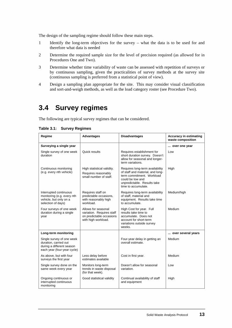
3.4 Survey regimes The following are typical survey regimes that can be considered. Table 3.1: Survey Regimes

Regime Advantages Disadvantages Accuracy in estimating waste composition

Surveying a single year ... over one year

Single survey of one week duration

Quick results Requires establishment for short duration survey. Doesn’t allow for seasonal and longer-term variations.

Low

Continuous monitoring (e.g. every nth vehicle)

High statistical validity. Requires reasonably small number of staff.

Requires long-term availability of staff and material, and long-term commitment. Workload could be low and unpredictable. Results take time to accumulate.

High

Interrupted continuous monitoring (e.g. every nth vehicle, but only on a selection of days)

Requires staff on predictable occasions, with reasonably high workload.

Requires long-term availability of staff, material and equipment. Results take time to accumulate.

Medium/high

Four surveys of one week duration during a single year

Allows for seasonal variation. Requires staff on predictable occasions with high workload.

High Cost for year. Full results take time to accumulate. Does not account for short-term variations outside survey weeks.

Medium

Long-term monitoring ... over several years

Single survey of one week duration, carried out during a different season each year (four-year cycle)

Four-year delay in getting an overall estimate.

Medium

As above, but with four surveys the first year

Less delay before estimates available

Cost in first year. Medium

Single survey done on the same week every year

Monitors long-term trends in waste disposal (for that week).

Doesn’t allow for seasonal variation.

Low

Ongoing continuous or interrupted continuous monitoring

Good statistical validity Continual availability of staff and equipment

High


Other regimes may be developed to suit user needs. The Ministry for the Environment’s EPI programme is currently developing reporting regimes for indicator measurement. Contact the Ministry for further information on this. Estimating the accuracy of various extended-duration surveys is not possible in the absence of previous data spanning a long time period. The information on survey design provided in Procedure Two can also be used as a guide to the accuracy of extended-duration sampling in representing the waste stream over the period of the survey, assuming there is no significant variation with time. It is only possible to assess the accuracy of the survey in representing long-term changes in the waste stream by analysing actual data collected in a specific situation.

3.5 Recommended survey regime

The following approach is recommended for the overall sampling regime.

• Surveys should be carried out over a minimum period of one week.

• Seasonal variation should be allowed for by repeating the survey at different times of the year. This would generally be best done over a week in the middle of each of the four seasons, but local variations such as circumstances over holiday periods may mean that this needs to be modified.






4 Procedure One: Classification of Domestic Wastes at Source

This procedure is summarised in section 3 of Appendix 1.

4.1 Purpose The purpose of the domestic waste survey is to obtain a quantitative estimate of the composition of solid waste from domestic premises within the survey area. Sampling at ‘source’ (at the individual household level) has the advantage of allowing statistics on waste generation per household to be derived. Recording where the waste is sampled allows waste generation statistics to be linked to other factors, such as average property size or socioeconomic indicators. Sampling at source is also more likely to give representative results (Musa and Ho 1981). This procedure can be used to assess the composition of the domestic waste stream or, in conjunction with a Procedure Two survey, provide data on the domestic waste stream as part of the overall waste stream.

4.2 Overview This procedure describes a direct manual sorting protocol for classifying refuse put out for municipal collection. The method involves:

collecting refuse put out for municipal collection from selected ‘households’ (this may include refuse put out by small commercial premises.)

•

•

•

•

•

transporting the refuse samples to a sorting station

sorting the refuse into 12 primary categories

weighing, and recording the information

statistical analysis and reporting. The methodologies for Procedures One and Two have a number of similar aspects (including sorting of refuse, weighing and recording of information, analysis and reporting). This procedure is written as a complete outline and repeats some material given in Procedure Two.


4.3 Survey design

4.3.1 Survey objectives

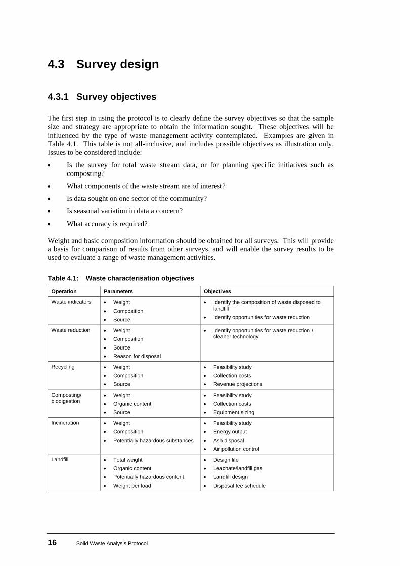
The first step in using the protocol is to clearly define the survey objectives so that the sample size and strategy are appropriate to obtain the information sought. These objectives will be influenced by the type of waste management activity contemplated. Examples are given in Table 4.1. This table is not all-inclusive, and includes possible objectives as illustration only. Issues to be considered include:

Is the survey for total waste stream data, or for planning specific initiatives such as composting?

•

•

•

•

•

What components of the waste stream are of interest?

Is data sought on one sector of the community?

Is seasonal variation in data a concern?

What accuracy is required? Weight and basic composition information should be obtained for all surveys. This will provide a basis for comparison of results from other surveys, and will enable the survey results to be used to evaluate a range of waste management activities. Table 4.1: Waste characterisation objectives

Operation Parameters Objectives

Waste indicators • Weight • Composition • Source

• Identify the composition of waste disposed to landfill

• Identify opportunities for waste reduction

Waste reduction • Weight • Composition • Source • Reason for disposal

• Identify opportunities for waste reduction / cleaner technology

Recycling • Weight • Composition • Source

• Feasibility study • Collection costs • Revenue projections

Composting/ biodigestion

• Weight • Organic content • Source

• Feasibility study • Collection costs • Equipment sizing

Incineration • Weight • Composition • Potentially hazardous substances

• Feasibility study • Energy output • Ash disposal • Air pollution control

Landfill • Total weight • Organic content • Potentially hazardous content • Weight per load

• Design life • Leachate/landfill gas • Landfill design • Disposal fee schedule


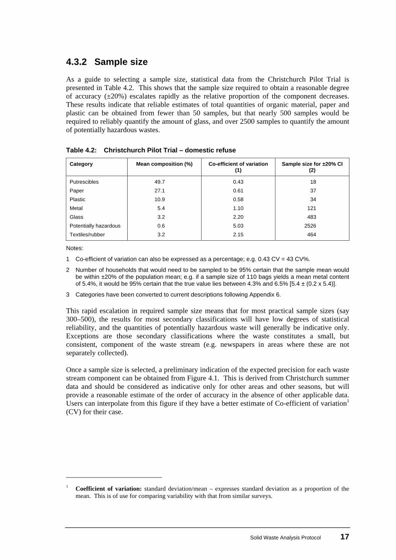
4.3.2 Sample size

As a guide to selecting a sample size, statistical data from the Christchurch Pilot Trial is presented in Table 4.2. This shows that the sample size required to obtain a reasonable degree of accuracy (±20%) escalates rapidly as the relative proportion of the component decreases. These results indicate that reliable estimates of total quantities of organic material, paper and plastic can be obtained from fewer than 50 samples, but that nearly 500 samples would be required to reliably quantify the amount of glass, and over 2500 samples to quantify the amount of potentially hazardous wastes. Table 4.2: Christchurch Pilot Trial – domestic refuse

Category Mean composition (%) Co-efficient of variation (1)

Sample size for ±20% CI (2)

Putrescibles 49.7 0.43 18 Paper 27.1 0.61 37 Plastic 10.9 0.58 34 Metal 5.4 1.10 121 Glass 3.2 2.20 483 Potentially hazardous 0.6 5.03 2526 Textiles/rubber 3.2 2.15 464

Notes:

1 Co-efficient of variation can also be expressed as a percentage; e.g. 0.43 CV = 43 CV%.

2 Number of households that would need to be sampled to be 95% certain that the sample mean would be within ±20% of the population mean; e.g. if a sample size of 110 bags yields a mean metal content of 5.4%, it would be 95% certain that the true value lies between 4.3% and 6.5% [5.4 ± (0.2 x 5.4)].

3 Categories have been converted to current descriptions following Appendix 6. This rapid escalation in required sample size means that for most practical sample sizes (say 300–500), the results for most secondary classifications will have low degrees of statistical reliability, and the quantities of potentially hazardous waste will generally be indicative only. Exceptions are those secondary classifications where the waste constitutes a small, but consistent, component of the waste stream (e.g. newspapers in areas where these are not separately collected). Once a sample size is selected, a preliminary indication of the expected precision for each waste stream component can be obtained from Figure 4.1. This is derived from Christchurch summer data and should be considered as indicative only for other areas and other seasons, but will provide a reasonable estimate of the order of accuracy in the absence of other applicable data. Users can interpolate from this figure if they have a better estimate of Co-efficient of variation1 (CV) for their case.

1 Coefficient of variation: standard deviation/mean – expresses standard deviation as a proportion of the

mean. This is of use for comparing variability with that from similar surveys.


Figure 4.1: Precision versus sample size for domestic waste stream components

TEXTILES/RUBBER

PUTRESCIBLES

Source: Christchurch Pilot Trial (Street 1992).

Note: Classification descriptions have been converted to current classifications following Appendix 6. Practical sample sizes are considered to be 300 to 500 households. This will yield precisions of around 5–10 % for the three major constituents (organic, paper, plastic), a precision of about 10–15% for total metal, and precisions of 20–30% for total glass and ‘other’ categories. Quantities of potentially hazardous waste will be indicative only. Where greater precision is required, the sample size should be increased.


4.3.3 Sampling strategy

For statistical efficiency a simple random sample is usually best. However, as this would result in sample households scattered over the refuse catchment, a systematic sampling procedure is recommended. Ideally this would be achieved by sampling every ‘ith’ household where ‘i’ is chosen to give the required total number of samples. A sample collection vehicle would run just ahead of the refuse truck to collect samples. This is the recommended strategy for smaller centres.

Sampling in larger centres

For larger centres, especially those with three or more collection trucks operating at a time, the operational efficiency of the above sampling strategy reduces. This is due to the number of teams required to follow each route to collect samples, and the long intervals between the collection of samples (‘i’ becomes a relatively large number). In larger centres, therefore, the sampling strategy can be modified to incorporate a cluster sampling technique. In this method ‘n’ collection routes or portions of collection routes are selected for sampling and, every, ‘ith’ household is sampled. In this case ‘i’ is chosen to enable the team to comfortably retrieve samples while remaining ahead of the collection truck (typically it takes one minute to collect a sample of bagged refuse). An example of a cluster sampling strategy in a metropolitan area would be to collect refuse from every 50th household on each of five randomly selected routes for each day of the week. Assuming 800 households per route, this would yield 400 households in total (5 x 5 x 800/50). A drawback of cluster sampling is that it involves the complication of selecting the clusters to be sampled. Inappropriate selection of clusters can lead to biased results. For instance, results from trials undertaken by Auckland City in 1990/91, and from the Taranaki Pilot Trial, indicate that refuse quantity and composition can be related to socioeconomic factors (Russell 1991; Taranaki Regional Council 1992a). Given the tendency for geographic grouping of households of similar socioeconomic status, it is important to ensure that the cluster samples come from a representative range of socioeconomic areas. Not less than six cluster samples should be taken (six routes or route portions), and preferably 10 or more. Advice should be sought from an experienced statistician where cluster sampling is used.

Stratified sampling

Where a town has distinctly different socioeconomic areas, it may be appropriate to use a stratified sampling technique. The areas are treated as separate statistical populations and are sampled individually. The results for the overall town are obtained by scaling up the number of households in each suburb. For optimum results, the amount of sampling effort put into each sub-population should be proportional to the product of population size and the standard deviation within the stratum. However, in general, the same sampling rate can be used satisfactorily in each stratum in order to simplify analysis. Advice should be sought from an experienced statistician where stratified sampling is used.


Non-bagged collections

Sampling at source is more difficult where refuse bags are not used. The survey team will need to be equipped with large, strong plastic bags into which to tip the refuse. Extra time for sampling should be allowed.

Sampling at point of disposal

Sampling at the point of disposal has limitations in terms of the information obtained and is therefore not recommended. Where information on variation between households is not required, this option has the advantage of being less expensive, but provides information on a bag/bin basis, not a household or source basis. Differentiating between residential and business bagged wastes is not usually possible. In addition, some rural collections pick up boxes and various containers as well as bagged/binned refuse. Sampling at the point of disposal can be undertaken by randomly selecting several bags off each of several randomly selected trucks. In this case the primary sampling unit is the truck. In estimating the survey precision, an unbiased estimate is formed for each truck, and then the variation between trucks is assessed. Information on the unsampled trucks, such as load weight, could be valuable in estimating the precision of the results. Separate counts of bags/bins per household would overcome some of the difficulties in assessing variation between households. Methodologies for sampling mixed domestic refuse (not bagged) at the disposal facility are similar to those used for sampling other mixed refuse at the disposal facility, as described in Procedure Two.

Two-tiered sampling

Where reliable data is required on only a particular component of the waste stream, a two-tiered sampling strategy can be employed. A sample of refuse from at least 50 households could be taken and classified to obtain a broad estimate of the composition of the waste stream for the 12 primary classifications. A much larger sample (possibly several thousand) could then be taken and sorted only for the particular commodity of interest. For readily identifiable components (e.g. plastic milk bottles), this method can quickly yield sufficient data to get a reliable result. A two-tiered sampling approach may also be used if you need to obtain an initial estimate of CV (in the first-tier survey) in order to design the full survey (as the second tier).

Coverage of collection service

In any collection area there may be more than one collection service available to the community. The various collection services may use different forms of container, with some related differences in the composition of refuse collected. The survey results should not generally be applied to users outside those of the collection service(s) surveyed.


Seasonality

Refuse production is seasonal. Four years of refuse data for Christchurch show a recurring pattern of reasonably consistent refuse production from January to May, a sharp fall to a yearly low in June, then a steady increase to the yearly peak in December. The December peak is typically 60% higher than the June low. Clearly a single survey of refuse produced in Christchurch in June or December would not yield accurate data on refuse quantity. A single survey at these times is also unlikely to yield an accurate estimate of composition, when seasonal factors such as gardening and leisure practices are taken into account. Seasonal variations will be even more marked in resort or holiday communities. In some communities, the temporary population over a holiday period can exceed the permanent population. Where accurate determinations of refuse composition or quantity are required, a sample of refuse should be taken in each of the four seasons. In the absence of continuous sampling, this is the recommended procedure where the protocol is to be used for accurate measurement of waste generation or against waste reduction goals. As a last resort, a single survey may need to be conducted at a representative time of the year. This representative time would have to be carefully selected. Annual estimates derived from a single survey should be considered as indicative only. Further information on sampling regimes and seasonality is contained in section 3. For resort areas there may be no representative time of the year. In these cases a stratified sampling approach may be appropriate, with the high and low seasons being treated as two distinct populations.

4.4 Set-up and training

4.4.1 Sorting logistics and equipment

The following equipment is required for sorting: •

•

•

•

•

•

• – – – – –

1 table, 2 m x 1 m minimum (larger tables are sometimes useful when sorting from MGBs) N bins for refuse classifications (one for each classification, labelled according to classification) 1 craft knife (or other tool to cut refuse bags) 1 dust pan and brush 1 broom 1 rake protective gear for each worker that consists of:

overalls gloves (leather or similar non-puncture outers with rubber surgical inner) eye protection dust mask suitable protective footwear


ear muffs •

•

•

•

•

•

weighing scales generator (if a power source is required) note pad, pens, calculator and pre-printed forms to record data first aid kit access to sanitation facilities.

A table not more than 1 m wide will allow operators to reach across the full width. If a larger table is used, care is needed when reaching across. Use plastic bins for holding and weighing classified refuse. Plastic bins that are used for kerbside recycling are a good size. The layout of the sorting area is not critical to the survey results, but can be very important for efficiency. The team should be free to alter the layout to obtain best efficiency. A variety of bin sizes will be required to handle the various quantities. These should be suitably located around the sorting table. Two levels of sorting bins will keep the maximum number of bins within an arm’s length of the sorter.


Figure 4.2: Typical domestic waste-sorting layout


4.4.2 Additional resource needs

In addition to the facilities and equipment for sorting and weighing, the following will need to be provided:

a suitable vehicle to collect the refuse bags for analysis •

•

•

•

•

•

•

•

•

•

•

•

•

tape for taping bags together, marker pens and labels

refuse bags where bags are not used for the collection service (a number of bags should also be available for other cases to deal with spillages)

a skip bin for tipping rubbish after sorting and weighing, or other provisions for collecting the rubbish.

4.4.3 Recruiting personnel

Selecting the appropriate personnel is critical to getting a reliable result. The work is not pleasant. Most personnel rapidly overcome this difficulty, but for some the task remains offensive for cultural or other reasons. Best results will be obtained if all personnel are committed to the ethic of obtaining sound data for good environmental decision making, and if they have an interest in environmental issues.

4.4.4 Health and safety

Sorting through waste can be dangerous. Care is needed to ensure that the health and safety of survey personnel are protected. The requirements of the Health and Safety in Employment Act must be met in any workplace. As an employer, it is presumed that any organisation undertaking a protocol survey will have in place procedures for complying with this Act. Health and safety procedures for a protocol survey should conform to the employer’s general procedures. Before commencing the survey a health and safety plan for the survey should be prepared, with consideration given to the following aspects:

the organisation’s health and safety policy, including management accountabilities for health and safety at work

safety training procedures

the procedure for supervising employees and sub-contractors

safety management organisation and accountabilities

safety personnel, including responsibilities and contact details

procedures for training on the proper use of work equipment and substances

procedures for identifying and assessing hazards, and for the avoidance or control of risks to the safety and health of employees and others

procedures for recording and investigating work injuries and subsequent revision of the hazard assessments and risk avoidance or control measures

procedures for dealing with emergencies that may arise while employees are at work


procedures for monitoring health and safety performance •

•

•

•

•

•

•

•

•

•

•

•

•

procedures for monitoring the health and safety of employees where they are exposed to hazards at work

provision of protective equipment that is appropriate to the risks employees and others may be exposed to while at work

such other health and safety issues as are considered appropriate. The Health and Safety Plan should also include a written assessment of hazards for the survey work and the measures to be taken to eliminate, isolate or minimise these risks. First aid kits should be available at the survey site, and at least one member of the team should hold a current first aider’s certificate. The organisation undertaking the survey is responsible for identifying hazards. This should normally involve the survey staff. The following list of potential hazards is intended solely as a guide. A specific assessment should be done for each survey, taking account of the specific environmental conditions and the nature of the survey:

traffic (when collecting refuse) lifting heavy objects dust sharp objects in the waste exposure to decomposing wastes exposure to medical wastes inhalation of solvent fumes mixing of materials to form hazardous reactions or substances exposure to a variety of potentially hazardous wastes.

It is important that the survey team undergo health and safety training so that they are prepared and aware of potential hazards. Nearly anything can be hidden within refuse – from toxic chemicals to unprotected syringes. It is important to take a precautionary approach to handling wastes. Where there is any concern about handling a particular material, that material should not be handled, and should be isolated and disposed by the safest available means, and an estimate made of the quantity and type of waste for the purposes of the survey. In general, waste materials should remain in their container unless it is necessary for the sort-and-weigh survey that they be removed, and it is clear that no hazard is likely to be caused in doing so. Care should be taken when opening any container or wrapping if the contents cannot be checked without being spilled. The container/wrapping should be resealed if necessary. Advice and assistance from disposal site operators or other available people with experience in waste disposal should be sought if surveyors are unsure about the safe handling of any waste material. Where a hazardous material is identified and the material type is known, the relevant manufacturer’s Material Safety Data Sheet should be referred to for guidance on safe handling and disposal.


Health and safety measures to be implemented may include:

ventilation of the sorting area •

•

•

•

•

•

•

•

•

•

•

•

•

•

•

•

•

•

•

safety clothing for personnel (see section 4.5.1)

measures for containment and disposal of leaking containers – including soil for containment, bags or other containers for the leaking container

containers for the safe disposal of sharps where these cannot safely be left in the mixed refuse (e.g. hypodermic needles)

wash-down water for diluting spills on the site, or on equipment and clothing

antiseptic soap and washing facilities

rags or other methods for clean-up of minor spills

contact details available on the survey site for specialist advice and emergency services

suitable facilities for meal breaks, away from the sorting area. It is important that all workers are up-to-date on their tetanus vaccination. Hepatitis vaccinations are not normally essential, as waste is not normally considered to be a high-risk exposure medium. Current medical advice should be sought regarding this and the need for any other vaccinations. Inoculation against hepatitis can take many months to be administered and can have undesirable side effects. Workers should take every precaution to avoid contact with blood products. Post-exposure treatment of hepatitis is available. If there are any health concerns, workers should immediately consult a physician.

4.4.5 Training

One day’s training for survey staff should be adequate. In addition to trial sorting of refuse at the refuse station, training should cover:

reasons for the survey how the survey fits into the bigger picture of waste management the survey procedure health and safety issues, including the use and care of equipment provided why sound / high-quality data is required reasons for the classifications that have been chosen the need for confidentiality.

Personnel should be provided with notes on what classifications various materials should go into. Particular attention should be given to:

differentiating between secondary classifications (e.g. the different types of newsprint / printed paper

identifying different types of plastic (if sub-classifying plastics)

classifying multi-media products (e.g. window envelopes, discarded appliances). The recommended rule is to classify multi-media products by the constituent of greatest mass.


4.5 Survey execution

4.5.1 Survey procedures

Sample collection

Samples should be collected just ahead of the normal refuse collection. Bags should be labelled to separate refuse from each household when they are collected (e.g. a consecutive number for each household). Where a household puts out more than one bag, each bag should be labelled and the bags taped together. Where bags are not used as part of the collection service, refuse from the containers used (e.g. MGBs) should be emptied into strong plastic bags provided for the survey. All refuse should be collected, separately contained, labelled, and sorted by household. The sample collection team should have tape to bundle multiple bags from an individual household, and to seal bags to prevent spillage. The team should also carry some spare bags in case refuse bags split when being handled. It is important that confidentiality be maintained to the greatest degree practicable. For this reason it is recommended that:

the identifiers correlating refuse with households be something other than street address •

•

•

all refuse collected and classified goes immediately back into the refuse stream confidentiality is emphasised to personnel and in any dealings with householders.

Sorting and weighing

Refuse bags should be weighed before sorting and the sum of weights after sorting checked against this. The refuse from each household should be sorted into the primary categories, and each category weighed and the weight recorded to the nearest 10 g. Refuse should then be similarly sorted and weighed by secondary categories, where applicable. Sample forms for use in Procedure One surveys are included in Appendix 10. Form A is intended for use where secondary classification is surveyed; Form B where only primary classifications are surveyed. These forms are examples only and other forms can be developed to suit individual needs. The simplest check on data entry are the totals before and after sorting. The system of double entry of data will identify most errors. This check should be made before tipping refuse into the waste bin so that any re-measurements can be made. Where any errors cannot be corrected, those measurements should not be included in the survey data. Refuse from residential properties and businesses can be recorded separately where this information is known. Sorted refuse should be disposed of to the appropriate disposal site. A skip bin or similar is recommended at the sorting area for tipping of sorted refuse.


4.5.2 Personnel productivity

In the Whangateau pilot trial it was found that a team of six workers could efficiently process about 30 bags of domestic garbage an hour to eight classifications (five bags per hour per worker). In the Taranaki pilot trial, two classifiers could deal with 10 to 15 bags per hour (5 to 7.5 bags per hour per worker). In the Christchurch pilot trial a team of four workers collected at source and separated domestic refuse at an overall rate of 5.6 households per hour. The extra effort of sorting to secondary sub-classifications does not appear to be high. In an analysis of North Shore refuse conducted by Auckland University it was found that a team of four sorters could classify 100 bags of refuse to around 40 classifications in 2 to 2.5 hours (10 to 12.5 bags per worker per hour) (WAP 1992)

4.5.3 Weighing

Scales must be accurate enough to reliably weigh the contents of the lightest bins, yet have sufficient range to cater for the heaviest items to be weighed. Typical weight ranges are shown in Table 4.3. The advantages and disadvantages of various scales are listed in Appendix 13. A typical set-up may be accurate scales of 0–10 kg capacity, supplemented by a larger-capacity, less accurate scale for an overall check on the totals of refuse prior to sorting (see Appendix 13 for typical weight ranges). Alternatively, a single industrial electronic scale capable of weighing up to 70 kg by 20 g increments may be hired. Bathroom scales are not recommended due to their inaccuracy. Scales should be checked using known weights before the survey and at the beginning of each day. The total mass of refuse from each sample should be weighed prior to sorting as a check against the individual fractions. All fractions should be weighed and totalled to check against the original mass. Tare weights must be obtained for each container. These should be checked daily as part of the start-up procedure. Table 4.3: Typical weight ranges of refuse collection containers

Weight Refuse container

Typical Maximum

Required accuracy

Bagged refuse 5–10 kg 20 kg 100 g

120 litre MGB refuse 10–15 kg 50 kg 100 g

240 litre MGB refuse 15–25 kg 100 kg 200 g

Classified refuse 0.05–10 kg 70 kg 10 g


4.5.4 Moisture content

For simplicity this protocol does not require the determination of moisture content. Wet weighs are used for both analysis and presentation of results. Determination of moisture content is optional, and is only recommended for users who are undertaking one or more of the following activities:

considering incineration as a disposal option •

•

•

•

•

investigating landfill gas generation, decomposition rates or leachate volume assessment

comparing refuse statistics with commodity production statistics

quantifying seasonal effects

determining accurate refuse quantities. Typical moisture contents are shown in Table 4.4. Table 4.4: Percentage moisture content

Classification Estimated % as generated1 Christchurch %2

Organic:

• garden 51 48

• kitchen 39 43

Paper:

• newspaper 6.0 27

• cardboard 5.8 19

• other – 16

Plastic 2.0 13

Metal Nil Not determined

Glass Nil Not determined

Notes: 1 Estimates for British Columbia (Gartner 1991). 2 Data from Christchurch Pilot Trial (Street 1992). Before sorting, the refuse samples should be protected from rain, wind and direct sunlight. For moisture content analysis, representative samples of between 100 g and 500 g of the more highly variable components should be taken as soon as possible after sorting and weighing, and should be sealed in plastic oven bags. Samples should be dried in a laboratory oven at 77°C for 24 hours to assure complete dehydration and yet avoid undue vaporisation of volatile material (Vesilind and Reimen 1981, in Gartner Lee 1991). The laboratory oven used for drying should be equipped with an internal fan and vented to external air to minimise odour nuisance. Moisture content is calculated according to the following equation:

% MC = wet weight – dry weight x 100 wet weight – bag weight


4.6 Data analysis and reporting

4.6.1 Data analysis

Results from the survey should be entered into a suitable database. Any form of computer spreadsheet is suitable for the collation and analysis of data. Cross-checks of total weights should be made to verify correct data entry. All entry and manipulation of data should include check sums, as these will detect most errors. The mean percentage composition is determined for each by calculating the total weight of that constituent divided by the total weight of refuse sampled. (This is not equal to the average of the compositions of the individual samples.) Confidence intervals should be determined as an indication of the precision of the results. These can be determined by statistical analysis of the data. Results from using the SWAP should be presented with a 95% confidence interval. The confidence interval gives the range about the sample mean within which the mean of the parent population is expected to lie. For example, the Christchurch pilot trial found that the proportion of paper by weight in summer was 27.1 ± 2.3% (95% confidence interval). This tells the reader that the paper made up 27.1% by weight of the refuse sampled and that the true value for all municipal refuse collected in Christchurch was very probably (95% confidence) between 24.8% and 29.4%. The basic statistical unit is the household (not the bag). Analysis and reporting should be based on weight (not volume). Estimates of precision achieved in the survey are usually based on the variation between the basic statistical units (within strata in a stratified design). In anything but a simple random sample, statistical advice should be sought on the method of obtaining confidence intervals. (See below for an explanation of precision.) Care should be taken not to mislead the reader as to the range of applicability of the confidence interval. For example, it is preferable to state: “The proportion by weight of garden waste during the week of the survey was found to be 53 ± 5% (95% confidence interval). This week is believed to be representative of the summer as a whole.” Avoid saying, “The proportion by weight of garden waste during the summer was estimated as 53 ± 5% (95% confidence interval)”. Further information on data analysis is given in Appendix 12.

4.6.2 Reporting

As a minimum the report should identify the quantities by weight put out for disposal from each of the primary classifications, and the precision of the results, expressed as confidence interval (e.g. paper 37% ± 3% by weight at 95% confidence interval). Results at each level should be presented in graphical form. To facilitate interpretation and comparison of data, pie charts should be used to show the relative composition of the various classifications of waste. Confidence interval should be shown on the pie charts. Other chart types (e.g. bar charts) may help to compare data over time.


The report should include details of the execution of the survey, including:

date •

•

•

•

•

•

•

•

location

summary of staff and equipment

description of the site and its contributing area and waste stream

description of the type of collection service (including frequency, container, charging methods)

description of the proportion of properties serviced by the surveyed collection service, and the type of other collections available

survey procedures

the presence of any potential biases in the results (e.g. seasonal factors, weather conditions, special local events).

With regard to potentially hazardous wastes, the recommended report format should simply list the substances found. Grouping under secondary classifications will help comparison with those found in other studies. When reporting results a distinction should be drawn between precision and accuracy. ‘Precision’ is a measure of the variability of estimates of a measure. For instance, a very large sample could yield an estimated annual paper component of 26.2 ± 0.2% (95% confidence interval). This would be very precise. ‘Accuracy’ refers to how close the estimated value is to the true value; that is, how much ‘bias’ there is in the reported result. The above example would not be accurate if seasonal factors had not been taken into account and the true value was 22.2%. The procedures here identify the precision of the results of the survey.

4.6.3 Archiving

The records of the survey sampling and sort-and-weigh should be retained (and included in the report) so that the results of the survey can be used for future analysis if required. Whatever software is used in the analysis, one copy of the raw data should be made in some commonly available format, such as a spreadsheet, text or csv file. Items of data should be accurately described, and the survey methods by which the data was collected should be documented. Particular care should be taken to avoid future access to the data being reliant on rare, expensive or unreliable proprietary products.


5 Procedure Two: Classification at Disposal Facility

This procedure is summarised in Section 4 of Appendix 1.

5.1 Purpose The majority of solid waste generated in New Zealand is transported to transfer stations or landfills. This section describes a procedure for characterising solid waste that arrives at the disposal facility in bulk. It can be used as the sole survey method, or in conjunction with a Procedure One survey providing data on the whole domestic waste stream – in this case trucks delivering waste from domestic collection would not be for waste composition.

5.1.1 Overview

This protocol emphasises the role of statistical analysis in the design of surveys and analysis of the results. Statistical analysis provides managers with an indication of how much they can rely on the results in decision making. The application of statistical principles in survey design enables users to get the most precise results for the least effort. Procedure Two entails:

weighing all or most large vehicle loads entering the site and a proportion of smaller vehicle loads

•

•

•

•

sampling a proportion of incoming loads in each category and sorting and weighing a sample of refuse from these

sorting the refuse

statistical analysis and reporting. A number of aspects of the methodologies for Procedures One and Two are the same (including sorting of refuse, weighing and recording of information, analysis and reporting). This procedure is written as a complete outline and repeats some material in Procedure One.


5.2 Survey design

5.2.1 Survey objectives

The first step in using the protocol is to clearly define the survey objectives so that the sample size and strategy are appropriate to obtain the kind of information sought. The type of waste management activity contemplated will influence these objectives. Examples are given in Table 5.1. This table is not all-inclusive and includes possible objectives as illustration only. Issues to be considered include:

• Is the survey for total waste stream data or for planning specific initiatives such as composting?

• What components of the waste stream are of interest?

• Is data sought on one sector of the community?

• Is seasonal variation in data a concern?

• What accuracy is required? Weight and basic composition information should be obtained for all surveys. This will provide a basis for comparison of results from other surveys, and will enable the survey results to be used to evaluate a range of waste management activities. Table 5.1: Waste characterisation objectives

Operation Parameters Objectives

Waste Indicators • Weight

• Composition

• Source

• Identify the composition of waste disposed to landfill

• Identify opportunities for waste reduction

Recycling • Weight

• Composition

• Source

• Feasibility study

• Collection costs

• Revenue projections

Composting/ biodigestion

• Weight

• Organic content

• Source


• Collection costs

• Equipment sizing

Incineration • Weight

• Composition

• Potentially hazardous substances


• Energy output

• Ash disposal

• Air pollution control

Landfill • Total weight

• Organic content

• Potentially hazardous content

• Weight per load

• Design life

• Leachate / landfill gas

• Landfill design

• Disposal fee schedule


5.2.2 Survey location

This procedure is written for use at a disposal site. This may include a transfer station, landfill, incineration plant, or other bulk waste-handling facility. To get a complete view of the waste stream in an area it may be necessary to consider Procedure Two surveys at more than one location. For instance, where part of the waste stream at a landfill comes from a transfer station, a Procedure Two survey could be done solely at the landfill site and include waste transported from the transfer station. If more detailed information is wanted on the source and manner of delivery of the waste, it may be appropriate to consider a separate survey at the transfer station site. The method of measurement of recycled material should also be considered. This may require:

measurement of recyclable material separated at the disposal site, where this takes place (the quantity of material recycled at the disposal site should be separately identified)

•

• measurement of the quantity of recyclable material that does not pass through the disposal site.

The simplest point to measure the recycling stream is at the recycling point of purchase, where the recyclable material has been collected in bulk. This means the number of firms that have to be contacted is kept to a minimum and all involved should therefore be contacted. Since most materials are purchased by weight, the recycling industry has reasonable records. A form similar to the form for a survey at a disposal site can be used. This form can be mailed out with a suitable covering letter and reply-paid envelope. Follow-up by phone will help to obtain a 100% return rate. Due to the commercially sensitive nature of this information, confidentiality is important throughout. The data obtained is useful to determine the potential to improve recycling of a particular material and the possible effects on the market. It also provides information on the success of waste minimisation programmes.

5.2.3 Load and source categories

Load categories

A typical refuse disposal facility will receive loads each day from many cars and vans, many trailers, and fewer trucks. Figures 5.1 to 5.4 from the Christchurch and Balcairn Pilot Trials illustrate this. Balcairn serves a rural area of approximately 2400 people, while Christchurch is urban and serves approximately 290,000 people. Given that the few trucks deliver as much or more refuse than many cars, a more accurate overall result will be achieved if a greater proportion of trucks is sampled.


Figure 5.1: Balcairn landfill: total weight of refuse per week, by vehicle type

0.9

11.1

0

8.7

0

2

4

6

8

10

12

Totalweight(tonne)

Cars Trailers Trucks Municipal refusetrucks

Vehicle types

Figure 5.2: Balcairn landfill: number of vehicles per week

12

43

03

0

5

10

15

20

25

30

35

40

45

Numberper week


Vehicle types


Figure 5.3: Christchurch transfer stations: total weight of refuse per week, by vehicle type

188

33

1648

350

1727

1338

850

0

500

1000

1500

2000

2500

3000

3500

Totalweight(tonne)


Vehicle types

Total weight per week (res)Total weight per week (bus)

Figure 5.4: Christchurch transfer stations: number of vehicles per week

2939

5349

1513

261

0

1000

2000

3000

4000

5000

6000

Numberper week


Vehicle types

It is therefore appropriate to segregate the incoming population of loads into sub-populations according to the size of vehicle. These sub-populations are sampled individually, and overall totals are calculated by scaling up the survey results in proportion to the total weight of refuse in each load category. The load categories recommended in this protocol are listed in Table 5.2 on the following page.


Table 5.2: Load categories

Category Code Vehicle types

Car C Car Station wagon / SUV

Trailer/utilities T Van Utility Trailer Tandem trailer

Truck Tr Skips / bins Trucks Compactor trucks

Division into further categories may be used where this is needed to separate loads by different overall composition. For instance, this could include separating trucks into two categories of under or over 3500 kg tare weight where it is likely that different truck sizes are a significant proportion of users and are likely to carry different kinds of refuse.

Refuse source categories

The second key identifier for refuse loads is source – whether residential or business. This basic classification of refuse source is a key identifier used in analysing the data collected. Residential refuse is predominantly transported by car and trailer, representing around 80% by weight of refuse delivered in these two categories in Christchurch. Business refuse is predominantly transported by truck (Figure 5.3). Rural landfills receive few trucks. Additional information on load source may be collected from the vehicle drivers if required for the survey objectives. Examples of possible additional information include:

•

– – –

•

– –

residential type of dwelling (house/flat/townhouse) number of occupants section size

business business name nature of business (to enable categorisation to basic levels of NZ Standard Industrial Classification).

5.2.4 The survey plan and the sampling plan

An essential part of any survey is the production of a written survey plan. The purpose of the survey plan is to document how the survey has been designed, and how it is to be executed. Documenting the survey design provides an opportunity to reflect on the design, to consider whether the survey is likely to meet the desired objectives, and to consider whether there are likely to be any biases in the results.


Survey method

There are two survey methods described in the Procedure Two methodology: sort-and-weigh •

• visual classification. The sort-and-weigh methodology has the advantage of greater accuracy and reliability in assessing the waste composition of each load of waste. However, it is time consuming and the number of waste loads able to be surveyed by this method is limited by the practicalities and costs of the method. Visual classification is easier and quicker. It makes the results of the survey more representative of the overall waste stream by allowing a greater number of waste loads to be surveyed so that the data set is more extensive than is likely to be affordable using just a sort-and-weigh methodology. However, the method is less accurate in assessing the composition of each load of waste. Visual classification also potentially introduces a bias in the measurement of proportions for individual survey staff. It is recommended that only the sort-and-weigh methodology be used for Protocol Two surveys. A Procedure Two survey can be designed to use both methods, but if visual classification is to be used then it must be in conjunction with sort-and-weigh methods, so that the accuracy of the visual classifications can be verified. Guidance in the use of visual classification is included in Section 5.4.8 to allow for this scenario. Further information on allocating the survey effort and selecting the sample size is provided in the following sections.

Sampling plan

A key component of the survey plan is the sampling plan. This is written for the staff executing the survey, and tells them what activities they are to undertake, and what effort should be allocated to the various activities and local categories. The sampling plan should aim to reduce bias by rotating the selected load category by time of day and day of week. Table 5.3 shows an example of a sampling plan. Table 5.3: Sampling plan: load category roster, Christchurch Pilot Trial

Time Monday Tuesday Wednesday Thursday Friday

8.00–9.25 am Truck Truck Truck Truck Other 9.25–11.10 am Other Truck Truck Truck Truck 11.10 am–12.35 pm Truck Other Truck Truck Truck 1.05–2.30 pm Truck Truck Other Truck Truck 2.30–4.15 pm Truck Truck Truck Other Truck

Notes: Saturday and Sunday – cars and trailers only.

Source Christchurch Pilot Trial (MAF Consultancy Services, 1992a).


Tiered sampling

Where reliable data is required on only a particular component of the waste stream, a two-tiered sampling strategy can be employed. A sample of refuse from at least 50 vehicles could be taken and classified to obtain a broad estimate of the composition of the waste stream for the 12 primary classifications. A much larger sample (possibly several thousand) could be taken and sorted only for the particular commodity of interest. For readily identifiable components (e.g. plastic milk bottles), this method can quickly yield sufficient data to get a reliable result. A two-tiered sampling approach may also be used where you want to obtain an initial estimate of the coefficient of variation (CV) (in the first-tier survey) to then design the full survey (as the second tier).

5.2.5 Optimal allocation of sampling effort

Optimal allocation of sampling effort is dependent on: the weight of refuse in each load category •

•

•

the variability of refuse in each load category the time required to select and measure samples.

The optimal allocation of sampling effort will be obtained if the sample effort per load category is proportional to 111 tsw (where w1 is the fraction of weight of refuse in the ith category, s1 is the standard deviation in this category, and t1 is the time required to sort a load in this category). The allocation will only be optimal for the particular constituent of interest for which the standard deviation term applies (e.g. organic waste). Also, the exact values of w1, s1 (and even t1) are not known at the outset of a trial. However, the objective is to get an indication of how best to allocate effort rather than an exact allocation. For these purposes a broad assumption of equal variability within the load categories allows the standard deviation term to be dropped, and the parameters of w1 and t1 can be estimated from the results of other surveys (supplemented by vehicle counts at the facility, where available). Examples of applying this simplified approach for a metropolitan and a rural facility are presented in Tables 5.4 and 5.5. These indicate that only a small amount of effort should be allocated to sampling loads arriving in cars, with most effort directed at trailers and trucks. At small- to medium-sized facilities where car loads make up only 5 to 10% of the total weight of refuse, car loads could be allocated the lowest sampling priority (loads would only be sampled when no other load was available). If no carloads were sampled during the course of the survey, data from other surveys could be used to estimate total weight and composition based on a count of the number of carloads.


Table 5.4: Optimal allocation of sampling effort: metropolitan facility, sort-and-weigh survey

Load type Cars Trailers Trucks

Total weekly weight (t)1 188 1650 1730 Sort time (mins)2 20 30 60

11 tw 841 9037 13,400

Allocation of effort 3 4% 39% 58% Loads sorted 4 7 49 36 Total number of loads 5 2939 5349 1513 Proportion sorted 0.2% 0.9% 2.4%

Notes: 1 Christchurch data (MAF Consultancy Services, 1992b). 2 Sort time for team of four including sample selection. 3 Allocation =

)( ii

ii

tWtw

∈

(= 23,278)

4 Loads sorted = Allocation % x 250 mhrs x 60 mins 100 4 sort time (mins)

(assuming 250 man hours labour available). 5 Municipal refuse trucks are excluded from analysis as municipal refuse is classified at source (see

Module B/Procedure One). Table 5.5: Optimal allocation of sampling effort: rural landfill, sort-and-weigh survey

Load type Cars Trailers Trucks

Weekly weight (t)1 0.9 11.1 Nil Sort time (mins)2 20 30 60

11 tw 4 61 Nil

Allocation of effort 3 6% 94% Nil Loads sorted 4 1 9 Nil Total number of loads 5 12 43 Nil Proportion of loads sorted 8% 21% NA

Notes: 1 Balcairn data (MAF Consultancy Services 1992a). 2 Sort time for team of four including sample selection. 3 Allocation =

)( ii

ii

tWtw

∈

(= 65)

4 Loads sorted = Allocation % x 20 mhrs x 60 mins 100 4 sort time (mins)

(assuming 20 mhrs labour available). 5 Municipal refuse trucks are excluded from analysis as municipal refuse is classified at source (see

Module B/Procedure One). The analyses in Tables 5.4 and 5.5 indicate that for optimum allocation of sampling effort, a much smaller proportion of cars should be sampled than of trailers or trucks. In the design of a survey at a particular facility, approximate vehicle counts in each category should be obtained beforehand to provide a basis for survey design. This information can be readily obtained from historical records, gate receipts, vehicle counts by the facility operator, or by installing a traffic counter.


5.2.6 Number of samples

The number of samples needed – and hence the total effort required – is dictated by the required precision of the results and the variability of the refuse components of interest. To achieve a reasonable level of precision (±10% to 20% for the main waste categories), a sample size for sort-and-weigh of 300–500 vehicles is recommended. At small sites this may exceed the number of vehicles using the site over the survey period, and the sample size would be limited to the number of site users. Note that the precision of the survey is dependent on the sample size, and hence the sample size may be independent of the number of users of the disposal site. Coefficients of variation for refuse loads surveyed in the Christchurch Pilot Trial are presented in Table 5.6. To assist with the design of surveys, data from the trial has been analysed to identify the sample size that would be required to obtain a precision of ±20% for each primary waste category (95% confidence interval). The results, presented in Table 5.7, indicate sample sizes required for a precision of ±20%. Table 5.6: Coefficients of variation (%)

Trucks Trailers Cars

Res Bus Res Bus Res Bus

Paper 99 84 197 128 138 55 Glass 142 281 255 346 365 266 Metal 135 221 252 167 156 137 Plastic 110 136 181 173 127 143 Putrescibles 38 120 45 114 62 146 Potential hazard 133 444 320 234 299 186 Textiles/rubber 273 241 251 215 200 113 Rubble, concrete/timber 279 221 192 263 273 355

Data source: Christchurch Pilot Trial (MAF Consultancy Services, 1992b). Waste classifications have been converted to current classifications following Appendix 7. Table 5.7: Sample size for results (±20%)

Trucks Trailers Cars

Res Bus Res Bus Res Bus

Paper 97 70 389 155 190 30 Glass 203 789 649 1195 1330 706 Metal 183 491 635 280 242 188 Plastic 121 186 328 298 162 204 Putrescibles 15 144 20 129 39 213 Potential hazard 176 1974 1024 549 894 344 Textiles/rubber 747 583 629 464 398 128 Rubble, concrete/timber 776 487 369 692 745 1264

Data source: Christchurch Pilot Trial (MAF Consultancy Services, 1992b). Waste classifications have been converted to current classifications following Appendix 8.


The key results are as follows:

fewer than 40 samples in each load category would be needed to determine the putrescibles component of loads from residential sources

•

•

•

•

fewer than 100 loads would be required to quantify the amount of paper hauled from businesses by truck or car

between 100 and 350 samples would be required to quantify the amount of plastic

between 200 and about 1000 samples would be required to quantify the amounts of other constituents, with the exception of hazardous wastes.

Clearly, the costs of sorting and weighing a sufficient number of samples to obtain reasonably precise estimates is prohibitive for all but the most common refuse constituents (such as putrescibles and paper). Having selected a survey design, the method given in Appendix 12 can be used to estimate the precision of the resulting data (using coefficients of variation adopted from previous surveys or from those given in Table 5.6). Note that this estimate of precision relates to the individual survey in representing the true situation over the survey period; the issues related to the accuracy of the survey in representing the composition of waste over the long term are discussed in Section 3. At larger facilities visual classification can be used to economically extend the data set and thereby potentially increase precision. However, this increase in precision assumes that the measurements made by visual classification are not biased. If this is not the case then a survey using visual classification may be less accurate, even though the precision is shown to be greater. Examples of survey design presented in Appendix 12 illustrate the use of visual classification in addition to sort-and-weigh. In these examples, the use of visual classification results in a threefold increase in precision. The effect of sample size on precision for a range of coefficients of variation is illustrated in Figure 5.5.


5.2.7 Survey design examples

Examples of survey design methodologies are given in Appendix 12. Figure 5.5: Precision of composition data versus sample size (95% confidence interval)

Source: Gartue Lee (1991).


5.2.8 Seasonality

Waste production is seasonal. Four years of waste data for Christchurch show a recurring pattern of reasonably constant refuse production from January to May, a sharp fall to a yearly low in June, then a steady increase to a yearly peak in December. The December peak is typically 60% higher than the June minimum. Clearly a single survey of refuse produced in Christchurch in June or December would not yield an accurate estimate of refuse quantity. A single survey at these times is also unlikely to yield an accurate estimate of composition when seasonal factors such as gardening and leisure practices are taken into account. Seasonal variation will be even more marked in resort areas such as beach communities or ski resorts. Checks on seasonal effects can be made from a range of sources (Table 5.8). Table 5.8: Seasonality checks

Source Applicability to site Accuracy Ease Cost

Published data Poor Poor Good Low Questionnaires Fair Fair Fair Medium Existing records (gate receipts, weighbridge) Good Fair–good Fair Low–medium Seasonal sampling Good Good Poor High

Source: SCS Engineers 1978. Where accurate determination of annual refuse composition or quantity is required, a sample of refuse should be taken in each of the four seasons. In the absence of continuous sampling, this is the recommended procedure where this protocol is to be used for accurate measurement of waste generation or against waste reduction goals. As a last resort, a single survey may need to be conducted at a “representative” time of the year. This would have to be carefully chosen. Annual estimates derived from a single survey should be considered as indicative only. Further information on seasonality is given in section 3. For resort areas there may be no “representative” time of year. In these cases a stratified sampling approach may be appropriate, with the high and low seasons being treated as two distinct populations.

5.2.9 Disposal site catchment issues

Regionalisation of waste disposal is a trend that results in cross-boundary transport of waste and should be recognised in survey design. The following issues need to be considered.

A surveyed disposal site may receive refuse from more than one territorial local authority area. Joint funding arrangements may be needed for protocol surveys at such sites.

•

• Further information on the source of the waste may need to be sought in addition to whether the waste is from a business or residential source. This may require an additional level of reporting of results for the location (in territorial local authority area or other relevant description). The level of reporting of results would then be as follows (see section 5.5.4):


1 facility 2 source region 3 source business/residential 4 load (vehicle type).

•

•

•

•

•

•

•

• – – – – – –

•

•

•

•

•

•

•

Waste may be taken to a transfer station before going to a disposal site. For this refuse, sampling should done be at the transfer station in preference to surveying the consolidated waste at the disposal site. This will allow the source of waste loads to be identified.

5.3 Set-up and training

5.3.1 Sorting logistics and equipment

Equipment required will include: 1 table 2 m x 2 m N bins for refuse classifications (one for each classification and labelled with the classification) 1 craft knife (or other tool to cut refuse bags) 1 dust pan and brush 1 broom 1 rake 1 protective gear for each worker consisting of:

overalls gloves (leather or similar non-puncture outers with rubber surgical inner) eye protection dust masks ear muffs suitable protective footwear

weighing scales plywood base (2 m x 1 m) for weighing bulky, light material generator (if a power source is required and a mains supply is not available) note pad, pens, calculator and preprinted forms to record data first aid kit access to sanitation facilities (handwash, drinking water, sanitation) 2 tape measures.

Se up the weigh scales and sorting bins before the vehicles arrive. If the site is an unfenced area the weigh scales must be removed at night and set up again in the morning. The public needs to be aware of the survey, so signs at the entrance should advise this. Information distributed through the news media is also helpful.


5.3.2 Other equipment

In addition to the facilities and equipment for sorting and weighing, the following will need to be provided:

suitable vehicle scales if there is no weighbridge at the site •

•

•

cones and signs suitable to direct traffic and safely define a working area for vehicle weighing

note pad, pens, calculator and pre-printed forms to record data.

Information on vehicle scales is given in Appendix 13.

5.3.3 Weigh scales for sorting

Scales must be accurate enough to reliably weigh the contents of the lightest bins, yet have sufficient range to cater for the heaviest items to be weighed. The advantages and disadvantages of different scales are listed in Appendix 13. A typical set-up may be an accurate scale of 0–10 kg capacity, supplemented by a larger-capacity, less accurate scale for an overall check on the totals of refuse prior to sorting (see Appendix 13 for typical weight ranges). Alternatively, a single industrial electronic scale capable of weighing up to 70 kg by 20 g increments may be hired. Bathroom scales are not recommended due to their inaccuracy. Tare weights must be obtained for each container. These should be checked daily as part of the start-up procedure. The scales should be calibrated with certified weights at least before and after the survey, and checked at the beginning of each day.

5.3.4 Recruiting personnel

It is estimated that three to five staff will be required for undertaking a survey. The selection of appropriate personnel is critical to getting a reliable result. The work is not pleasant. Most personnel rapidly overcome this difficulty, but for some the task remains offensive for cultural or other reasons. No specialist skills are needed, but training of survey personnel will be necessary. Best results will be obtained if all personnel are committed to the ethic of obtaining sound data.

5.3.5 Health and safety planning

Sorting through waste can be dangerous. Care is needed to ensure that the health and safety of survey personnel are protected. The requirements of the Health and Safety in Employment Act must be met in any workplace. As an employer, it is presumed that any organisation undertaking a protocol survey will have in place procedures for complying with this Act. Health and safety procedures in respect of a protocol survey should conform to the employer’s general procedures.


Before commencing the survey it is recommended that a health and safety plan for the survey be prepared, and consideration should be given to including the following:

the organisation’s health and safety policy, including management accountabilities for health and safety at work

•

•

•

•

•

•

•

•

•

•

•

•

•

•

•

•

•

•

•

•

•

•

•

safety training procedures

the procedure for supervising employees and sub-contractors

safety management organisation and accountabilities

safety personnel, including responsibilities and contact details

procedures for training on the proper use of work equipment and substances

procedures for identifying and assessing hazards, and avoiding or controlling risks to the safety and health of employees and others

procedures for recording and investigating work injuries, and subsequent revision of the hazard assessments and risk avoidance or control measures

procedures for dealing with emergencies that may arise while employees are at work

procedures for monitoring health and safety performance

procedures for monitoring the health and safety of employees where they are exposed to hazards at work

provision of protective equipment that is appropriate to the risks employees and others may be exposed to while at work

such other health and safety issues as are considered appropriate. The health and safety plan should also include a written assessment of hazards for the survey work and the measures to be taken to eliminate, isolate or minimise these risks. First aid kits should be available at the survey site, and at least one member of the team should hold a current first aider’s certificate. The organisation undertaking the survey is responsible identifying hazards. This should normally involve the survey staff. The following list of potential hazards is intended solely as a guide. A specific assessment should be done for each survey, taking account of the specific environmental conditions and the nature of the survey:

traffic weather lifting heavy objects dust sharp objects in the waste exposure to decomposing wastes exposure to medical wastes inhalation of solvent fumes mixing of materials to form hazardous reactions or substances exposure to a variety of potentially hazardous wastes.


It is important that the survey team undergo health and safety training so that they are prepared and aware of potential hazards. Nearly anything can be hidden within refuse, from toxic chemicals to unprotected syringes. It is important to take a precautionary approach to handling any wastes. Where there is any concern about a potential hazard, that material should not be handled, and should be isolated and disposed by the safest available means, and an estimate made of the quantity and type of waste for the purposes of the survey. In general, waste materials should remain in their container unless it is necessary for the sort-and-weigh survey that they be removed and it is clear that no hazard is likely to be caused in doing so. Care should be taken in opening any container or wrapping that the contents can be checked without being spilled, and resealed if necessary. Advice and assistance from disposal site operators or other available people with experience in waste disposal should be sought where surveyors are unsure about the safe handling of any waste material. Where a hazardous material is identified and the material type is known, the relevant manufacturer’s Material Safety Data Sheet should be referred to for guidance on safe handling and disposal. Health and safety measures to be implemented may include:

ventilation of the sorting area •

•

•

•

•

•

•

•

•

safety clothing for personnel (see section 5.3.1)

measures for containment and disposal of leaking containers – including soil for containment, bags or other containers for the leaking container

containers for the safe disposal of sharps where these cannot safely be left in the mixed refuse (e.g. hypodermic needles)

wash-down water for diluting spills on the site, or on equipment and clothing

antiseptic soap and washing facilities

rags or other methods for clean-up of minor spills

contact details for specialist advice and emergency services available on the survey site

suitable facilities for meal breaks, away from the sorting area. An important requirement is that all workers be up-to-date on their tetanus vaccination. Hepatitis vaccinations are not normally essential, as waste is not usually considered to be a high-risk exposure medium. Current medical advice should be sought regarding this and the need for any other vaccinations. Inoculation against hepatitis can take many months to be administered and can have undesirable side effects. Workers should take every precaution to avoid contact with blood products. Post-exposure treatment of hepatitis is available. If there is any health concern, workers should immediately consult a physician.


5.3.6 Training

One day’s training for survey staff should be adequate. In addition to trial sorting of refuse at the refuse station, training should cover:

reasons for the survey •

•

•

•

•

•

•

•

•

•

•

•

how the survey fits into the greater picture of waste management the survey procedure health and safety issues, including the use and care of equipment provided why sound / high-quality data is required reasons for the classifications that have been chosen the need for confidentiality.

Vehicle arrivals are less frequent at the beginning and end of the day, so stagger the survey team’s start and finish times (two people can set up equipment each morning and two others tidy up in the afternoon). Personnel should be provided with notes on what secondary classifications various materials should go into. Particular attention should be given to:

differentiating between secondary classifications (e.g. the different types of newsprint / printed paper)

identifying different types of plastic (if sub-classifying plastics)

classifying multi-media products (e.g. window envelopes, discarded appliances). The recommended rule is to classify multi-media products by the constituent of greatest mass.

5.4 Survey execution

5.4.1 General procedures

Confidentiality

It is important that confidentiality is maintained to the greatest degree practicable. For this reason it is recommended that:

all refuse collected and classified goes immediately back into the refuse stream confidentiality is emphasised to personnel and in any dealings with the public.


Vehicle selection

The recommended method of selecting vehicle loads for each activity is to pick the next available vehicle once the team is ready, provided that the load category (truck/trailer/car) matches the requirements of the sampling plan. This procedure could introduce bias as vehicles with certain distinctive load compositions tend to visit landfills only at less busy times. If this situation exists, then these vehicles have a greater chance of being selected for classification. Where this problem is suspected, the vehicle loads concerned should be treated as a distinct sub-population (load category) in the collection and analysis of data, and a sample selected for this sub-population. Given the variability of refuse, there would need to be a reasonable number of loads concerned, and they would need to be of markedly different composition from the norm for the extra complication of analysing a sub-population to be worthwhile. For instance, in the Christchurch Pilot Trial, the data was analysed for differences in load weights between:

business and residential cars •

•

•

•

•

•

•

•

business and residential trailers weekend and weekdays.

While some statistically significant differences were found, these were small and were inconsistent between the three transfer stations. It was concluded that the expectation of marked differences in load weights was unfounded.

5.4.2 Productivity of recruits

The Christchurch Pilot Trial found that a team of four people could: sort and weigh three car loads per hour sort and weigh two trailer loads per hour sort and weigh one truck load per hour (including sample selection).

It was found that one person could:

visually classify about 16 car loads per hour visually classify about eight truck or trailer loads per hour.

Similar results were found in the Whangateau and New Plymouth pilot trials (Creese et al 1992; Taranaki Regional Council 1992b).


5.4.3 Data recording

A suitable form for collecting all data at the disposal facility is provided in Appendix 11. This form is an example only, and other forms can be developed to suit individual needs. The top section of the form will be filled out for all vehicles. The left-hand section is used for visual estimation of primary classifications for loads that are not sorted and weighed,– this is not a visual classification methodology referred to in sections 5.2.4 and 5.4.8. The information recorded may be useful in later review of results. The lower right-hand section is for recording sort-and-weigh data. Classification into the primary classifications is highly recommended. Classification to the secondary classifications is optional. The procedure for using the form is outlined as follows:

1 All vehicles Weight in/out:

• Vehicle weight: scale operator fills out weights on Form A from weighbridge or from scales.

• Source: cross out business or residential (if mixed load include % business). • Transport: circle appropriate vehicle type. 2 Visual estimation

• Check number of categories present on vehicle. • Take care not to overlook small parts of the load. • If all categories are present, be particularly careful with the estimate. • Check that your own visual estimation adds to 100%.

3 Sort-and-weigh • Weights to two decimal places (e.g. 60.64 kg). • % to one decimal place (e.g. 20.9). • Check % PRIMARY total adds to 100. • Check PRIMARY kg add to Nett ± 10%. 4 Feedback Evaluate differences between visual estimates and sort-and-weigh. Discuss

methodology and hints to improve.

5.4.4 Weighing vehicles

As many vehicles as possible should be weighed on arrival and on leaving the site. Where vehicles have known tare weights, these may be taken as the empty weight on leaving the site. Where all vehicles cannot be weighed, the number and type of vehicle should be recorded as the minimum for calculating total weights of refuse over the survey period. Estimate the percentage composition by weight of each waste category for all loads that are not to be sorted and weighed. This provides additional information on incoming refuse at the site – the measurement of waste composition is obtained from the sort-and-weigh samples.


5.4.5 Sorting and weighing

Sorting and weighing of the refuse is similar in methodology to the sorting and weighing of domestic refuse (Procedure One). The key difference is that a sample must first be taken for analysis. The recommended sampling strategy is shown in Table 5.9. Table 5.9: Sort-and-weigh sampling strategy

Category Typical load range (kg) Average1 load (kg) Recommended sampling strategy

Car 20–280 64 Full load Trailer 100–1600 310 Full load Truck 250–6000 1140 140 kg sub-sample

Note: 1 Data from Christchurch Pilot Trial (MAF Consultancy Services, 1992b). Ideally the sorting area should be covered and paved. Uncovered sorting areas can be used, but performance and data quality will be lower, and sorting may not be possible at all on days with continuous rain or strong wind. The sorting area needs to be at least 10 m x 10 m, with further areas available for storing refuse before and after sorting. If visually classifying loads, this should be done before sort-and-weigh of a sample. Weights of each component are recorded, together with approximate volumes if volumetric data is also being gathered. Tare weights only need to be measured once for vehicles that regularly haul loads to the landfill (if tare weights are not available, then reweigh the empty vehicle, record on form and retain form). When sorting and weighing the primary categories, the load must be weighed before sorting and the total after sorting checked against this. Weights should be recorded to the nearest 10 g. Sample forms are included in Appendix 11. Detailed sorting of mixed domestic waste is not generally recommended. For efficiency, it can be assumed that mixed domestic waste delivered to the facility is similar in character to the collected domestic refuse classified using the methodology presented in Procedure One. Where a Procedure One survey has not been done, or this assumption is not believed to be valid, and a particularly high degree of reliability of data is sought, some manual sorting using the sorting methodology outlined in Procedure One may be required. The sampling method described in section 5.4.6 can then be used to obtain a representative sample of large loads of loose mixed domestic refuse. Where the refuse is in bags, a sample of bags should be taken from throughout the load in a similar manner, to give a total sample weight of approximately 140 kg. The simplest check on data entry are the totals before and after sorting. The system of double entry of data will identify most errors. Refuse from residential properties and businesses can be recorded separately where this information is known.


5.4.6 Refuse sub-sampling

It is not generally practical to sort and weigh large loads of refuse, so it is necessary to obtain a representative sub-sample of part of the load that can then be measured by the sort-and-weigh method. The optimum size of a sub-sample for refuse classified at disposal facilities was found to be between 90 and 140 kg (Klee and Carruth 1970). Later investigators have also recommended a sub-sample size of 140 kg (Brittan 1972). In this protocol a sub-sample size of around 140 kg is recommended. A number of sub-sampling methods are available to ensure that a representative sample is obtained. A suitable method is illustrated in Figure 5.6. This technique is adequate provided that care is taken to avoid obvious sources of bias (such as continually taking scoops from the edge of the load where some constituents of refuse tend to segregate out). Where discrete large objects are included in the load (e.g. a tree stump), these should be separated from the remainder of the load, weighed, the balance of the load sub-sampled as described, and the results combined as the total measure of the load composition. An increase in the sample size may need to be made if the load is varied in composition, or if it contains a number of large items (e.g. construction wastes). For the Christchurch Pilot Trial, where there were safety and space considerations, a simpler approach was taken. The loader driver on the floor of the transfer station pit undertook the selection of sub-sample. When a sub-sample from a particular load was required, the load was spread out a little with the back face of the loader bucket, then a “scoop” of about 140 kg was sub-sampled from the load and delivered to the sorting platform. A similar approach was used in the New Plymouth Pilot Trial. There are potential biases associated with this technique and it is not recommended. A selection of at least six to seven parts to make up the 140 kg sample is preferred, as outlined in Figure 5.6.


Figure 5.6: Refuse sub-sampling


For trailers, the full load should be sorted and weighed irrespective of weight. Much of the effort involved in classifying trailer refuse is in unloading the material. The amount of extra handling in classifying the full load is relatively small, and helps to keep the procedure simple. The largest trailer loads tend to be homogeneous (e.g. all rubble or all soil). In these cases, classification may be undertaken by sorting and weighing only the minor constituents. The weight of the major constituent can then be determined by a simple subtraction from the overall load weight. Self-haul vehicles also bring the occasional bag of mixed domestic refuse. Sorting small amounts of bagged domestic refuse (or refuse from the municipal collection) is not recommended as part of this procedure. In this case, the weight of such refuse should be recorded but no composition analysis undertaken as appropriate composition data is collected under Procedure One or by measurement of refuse from the municipal collection (see section 5.4.5). Other refuse that happens to arrive in bags is weighed and classified.

5.4.7 Moisture content

For simplicity, this protocol does not require the determination of moisture content. Wet weights are used for both analysis and presentation of results. Determination of moisture content is optional and is recommended for users who are undertaking one or more of the following activities:

considering incineration as a disposal option •

•

•

•

•

investigations concerning landfill gas generation, decomposition rates or leachate volume assessment comparing refuse statistics with commodity production statistics quantifying seasonal effects determining accurate refuse quantities.

Some estimated moisture contents for products as generated, and moisture contents found in Christchurch municipal refuse, are presented in Table 5.10. Table 5.10: Moisture content (%)

Classification Estimated as generated1 Christchurch2

Organic:

• garden 51 48

• kitchen 39 43

Paper:

• newspaper 6.0 27

• cardboard 5.8 19

• other – 16

Plastic 2.0 13 Metal Nil Not determined Glass Nil Not determined

Notes: 1 Estimates for British Columbia (Gartner Lee 1991). 2 Data from Christchurch Pilot Trial (Street 1992).


Before sorting, refuse samples should be protected from rain, wind and direct sunlight. For moisture content analysis, representative samples of between 100 and 500 g for the more highly variable components should be taken for analysis. The samples should be taken as soon as possible after sorting and weighing, and sealed in plastic oven bags. After being opened, the bags can serve as trays during oven drying. Samples should be dried in a laboratory oven at 77oC for 24 hours to assure complete dehydration while avoiding undue vaporisation of volatile material (Vesilind and Reimen 1981, in Gartner Lee 1991). The laboratory oven used for drying should be equipped with an internal fan and vented to external air to minimise odour nuisance. Moisture content is calculated using the following equation:

% MC = wet weight – dry weight x 100 wet weight – bag weight

5.4.8 Visual classification

Visual classification is a method whereby an observer estimates the proportions of refuse belonging to the primary waste classifications. Visual classification yields far more data than sorting and weighing, but it is less precise. One person can visually classify 8 to 16 vehicle loads of refuse per hour; the limiting factor being the time to discharge loads. In comparison, a sort-and-weigh team of four people can process between one and three vehicle loads per hour. Visual classification typically yields 16 times more observations than sorting and weighing per unit of effort. However ,visual classification potentially introduces a bias into the survey results, as the data is dependent on observation rather than measurement. An individual or group of surveyors may tend to over- or underestimate in a set of results. There is also likely to be greater error in the data determined for each load and consequently a risk of less precision in the results. Calibration of visual classifications in some previous surveys has been poor, and resulted in users abandoning this method in order to achieve a reasonable level of accuracy. It is therefore recommended that Procedure Two surveys do not use visual classification methods. In some cases individual users may still wish to consider visual classification, and the following notes are intended for guidance in that situation. However, visual classification should only be used where calibration results against sort-and-weigh demonstrate that there is no bias in the composition data obtained.

Method

Visual classification is a method for quickly collecting a large amount of data. Only one person will be visually classifying loads at a time. This person will make their assessment of the load as it is being unloaded from the vehicle, so that the entire load is seen. It is useful to estimate major components first, then note which categories are not present, and finally estimate minor components. It is essential to check that the sum of the estimates is 100%. Major components should be recorded to the nearest 5%, while components less than 10% should be recorded more accurately. To reduce the likelihood of bias, each member of the survey team should be rostered on the visual classification daily.


All loads that are sorted and weighed in detail should also have estimates of visual classification done by the remainder of the survey team. Separate working sheets should be provided to each team member, to avoid them subconsciously using the previous team member’s estimate. Following calculation of weights, immediate feedback should be given to each team member on an individual basis. This helps team members improve their visual classifications. Where there is some doubt about the ability of personnel to be sufficiently accurate in visual classification, the survey design should be initially based on sort-and-weigh only. During the initial stages of the sort-and-weigh survey, visual classification of the refuse can be trialed at little extra effort. If the visual classification proves to be reasonably consistent, it can be used to augment the data set and thereby improve precision. Different people will need different amounts of calibration against sort-and-weigh before they can undertake visual calibration duties. This can be evaluated by plotting calibration results for each individual. The visual assessment of loads to be sorted and weighed should, of course, be carried on throughout the survey, so that these loads may be considered a representative selection of the total that was visually assessed.

Calibration

Visual classification cannot be reliably used without calibration against sorting and weighing. It can take some time for the survey team to “get their eye in”. Interest and motivation of the classifiers is also important to the success of the method. The pilot trial at Whangateau using postgraduate students found a high correlation between visual classifications and sort-and-weigh (Creese et al 1992). For the calibration it is recommended that at least 30 observations of visually classified refuse composition versus sort-and-weighed composition be obtained, including at least 15 per load category visually classified.

Applications

Typically, visual classification will be used in intensive studies at major metropolitan facilities. It can be used at smaller facilities without an extensive calibration period if a suitably experienced person, calibrated in other recent surveys, is engaged to visually classify the refuse. Visual classification is not suitable for minor refuse constituents (typically less than 5% of load), as these may be overlooked.

Analysis

In statistical terms, the use of calibrated visual classification is a double sampling technique. Plots of visual classification results against sort-and-weigh results for each commodity allow calibration lines to be determined. Ideally the relationship is a 45-degree line passing through the origin. This relationship indicates that no corrections are required to the statistical data generated from the visual classifications. If the plot of sort-and-weigh versus visual is not satisfactory, the visual classifications should be discarded and the analysis based solely on the sort-and-weigh data.


Benefits

The primary benefit of visual classification is that it enables a relatively high degree of precision to be achieved at reasonable cost. The results from a survey employing calibrated visual classification are expected to be up to three times more precise than a simple sort-and-weigh survey.

Weight or volume

Visual classification can be used to estimate either the weight or volume of the refuse. Given the adoption of weight as the basic measure of quantity in this protocol, visual classification to directly estimate weight is the preferred methodology. Visual classification by volume is not recommended due to the need to introduce “standard” densities to generate a weight figure. This creates a need for extra data manipulation, and thereby creates an opportunity for error. Volumetric data is especially relevant to operators who sell landfill space. However, the relationship between volume at the gate and volume in the landfill is not straightforward as it depends on the degree of compaction applied to the load.

5.5 Data analysis and reporting

5.5.1 Data analysis

Results from the survey should be entered into a suitable database. Any form of computer spreadsheet is suitable for the collation and analysis of data. Cross-checks of total weights should be made to verify correct data entry. All entry and manipulation of data should include check sums as these will detect most errors. Percentage composition should be determined for each constituent. The mean percentage composition for a constituent is determined from the total weight of that constituent divided by the total weight of refuse sampled. This is not equal to the average of the compositions of the individual samples. Confidence intervals should be determined as an indication of the precision of the results. Confidence intervals can be determined by statistical analysis of the data. Results from using this protocol should be presented with a 95% confidence interval. The confidence interval gives the range about the sample mean within which the mean of the parent population is expected to lie. For example, the Christchurch Pilot Trial has found that the proportion of paper by weight in summer is 27.1 ± 2.3% (95% confidence interval). This tells the reader that the paper made up 27.1% by weight of the refuse sampled and that the true value for 95% of all municipal refuse collected in Christchurch in summer is expected to lie between 24.8% and 29.4%. Confidence intervals can be determined by statistical analysis of the data.


Care should be taken not to mislead the reader as to the range of applicability of the confidence interval. For example, it is preferable to state: “The proportion by weight of garden waste during the week of the survey was found to be 53 ±5% (95% confidence interval). This week is believed to be representative of the summer as a whole”. Avoid saying: “The proportion by weight of garden waste during the summer was estimated as 53 ±5% (95% confidence interval)”. Further information is given in Appendix 12.

5.5.2 Data validation for visual classification (calibration)

If visual classification has been carried out, as well as sorting and weighing, the first step in the analysis is to check that the two methods are giving roughly similar answers. For this purpose:

1 create a separate database for all sort-and-weigh samples

2 for each of the major categories, plot sort-and-weigh (0–100%) against visual classification (0–100%)

3 the points should be scattered around the line y = x with no apparent tendency for a substantial majority of points to lie above or below the line for any substantial part of the range.

If all is well, proceed to the next section, using visually classified data in conjunction with sort-and-weigh. If all is not well, the visuals may need to be abandoned, and only sort-and-weigh data used in the next section.

5.5.3 Statistical analysis

A simplified statistical analysis is sufficient to derive composition and load weight data by source and vehicle. Standard deviations can be determined using commonly available computer spreadsheet software. Appendix 12 provides examples of the methods for statistical analysis. Relevant statistical parameters are described in the Glossary. The statistical analysis of the survey data will describe the accuracy of the data in measuring waste over an individual survey period. Accuracy of data in measuring waste over the long term will require a similar analysis of surveys undertaken at a different time (see section 3).


5.5.4 Reporting

To provide a basis for comparison with other surveys, results should be reported by source and vehicle type, as in Table 5.11. Table 5.11: Reporting: level of summary

Load Source Facility

Kerbside collection Cars Trailers Trucks

Business

Kerbside collection Cars Trailers Trucks

Residential

Treatment/disposal facility

Additional vehicle categories or source types may be added to suit local circumstances. Results at each level should be presented in graphical form. To facilitate interpretation and comparison of data, pie charts should be used to show the relative composition of the various classifications of waste. Confidence interval should be shown on the pie charts. Other chart types (e.g. bar charts) may help to make data comparisons over time. As a minimum the report should identify the quantities by weight put out for disposal from each of the primary classifications, and the precision of the results (expressed as confidence interval; e.g. paper 37% ± 3% by weight at 95% confidence interval). The report should include details of the execution of the survey, including:

date •

•

•

•

•

•

location summary of staff and equipment description of the site and its contributing area and waste stream survey procedures the presence of any potential biases in the results (e.g. seasonal factors, weather conditions, special local events).

With regard to potentially hazardous wastes, the recommended report format is simply to list the substances found. Grouping under secondary classifications will help comparison with those found in other studies. When reporting results a distinction should be drawn between precision and accuracy. ‘Precision’ is a measure of the variability of estimates of a measure. For instance, a very large sample could yield an estimated annual paper component of 26.2 ± 0.2% (95% confidence interval). This would be very precise. ‘Accuracy’ refers to how close the estimated value is to the true value; that is, how much ‘bias’ there is in the reported result. The above example would not be accurate if seasonal factors had not been taken into account and the true value was 22.2%. The procedures here identify the precision of the results of the survey.


5.5.5 Archiving

The records of the survey sampling and sort-and-weigh should be retained (and included in the report) so that the results of the survey can be used for future analysis if required. Whatever software is used in the analysis, one copy of the raw data should be made in some commonly available format such as a spreadsheet, text or csv file. Items of data should be accurately described, and the survey methods by which the data were collected should be documented. Particular care should be taken to avoid future access to the data being reliant on rare, expensive or unreliable proprietary products.


6 Quantity Estimates This section provides supplementary information on the assessment of total waste quantities over time. This is not a protocol procedure, but is intended to clarify the use and scope of the SWAP procedures.

6.1 Limitations on the use of SWAP survey data for total waste quantities

The SWAP methodology is for characterising the composition of the waste stream. Procedure Two can provide an accurate estimate of total waste quantities at the surveyed site for the period of the survey. Extrapolation of this information to estimate total waste quantities over a longer period (such as yearly), or to estimate total waste quantities in another period (such as in the following year) is unsound and inaccurate. Further explanation of issues relating to the accuracy of the SWAP methodology is given in Section 3. Where SWAP surveys are undertaken at regular intervals over a period of time, more reliable estimates of total waste quantities for that period can be obtained from the survey results. However, in the absence of this, other methods should be used to measure total waste quantities, and the SWAP used for assessing the composition of the total waste stream.

6.2 Methods to measure total waste quantities There is no requirement to adopt a protocol for measuring total waste quantities. A variety of methods are in use in New Zealand, depending on a variety of factors. Any measurement of total waste quantities by a means that includes all waste components will yield an estimate of waste quantities that can be compared with data from other locations and sources, providing the method of data collection is known. The waste classifications used in this protocol should be used where total waste quantity records are reported by different waste types. The following outlines the main methods that can be used for estimating total waste quantities at a disposal site.

6.2.1 Weighbridge records

Larger disposal sites commonly have weighbridges at the site entrance. Where records are kept of incoming waste quantities, this method can provide the best measurement of total waste quantities.


6.2.2 Ticket/till records

Vehicle numbers and types can be recorded at sites where there is no weighbridge but the site entrance is staffed, and an estimate made of the amount of waste carried by the incoming vehicles. Ticket or till records for payment of disposal fees can be adapted to record the type of vehicle and an assessment of the amount of refuse. This method should best be supplemented by periodic weighing of a sample of vehicles to determine the average waste quantity carried by vehicles of various types.

6.2.3 Vehicle numbers

Where disposal sites are not staffed, vehicle numbers entering the site can be counted using an automatic traffic counter. Alternatively, periodic manual counting of vehicles can be made to derive an estimate of the number of incoming vehicles. Methods are available for traffic classification counts to classify vehicles into principal types. This method should be supplemented by periodic weighing of a sample of vehicles to determine the average waste quantity carried by vehicles of various types.

6.2.4 Regular SWAP surveys

Where SWAP surveys are undertaken regularly, these results may be able to be used to estimate total quantities. The accuracy of the SWAP surveys over time can be determined from the actual survey results, to assess the validity of the surveys for estimating total quantities.

6.2.5 Landfill topographical survey

Topographical surveys of landfill contours can provide an estimate of the in-place volume of waste in a landfill. This method would need to be supplemented by records of quantities of landfill cover and by measurement of the in-place density of waste landfilling. Allowance is also needed for the reduction in volume with decomposition and consolidation of the refuse. This method is most suitable for monitoring proportional changes in waste quantities where base information on quantities is obtained by another method.

6.2.6 Waste transfer quantities

Where waste is accumulated at a transfer station for transfer in bulk to a disposal site, it may be practical to weigh the transfer vehicles to measure the total waste quantities.


References and Bibliography ACC. 1992. The Management of Hazardous Substances and Facilities. Auckland: The Department of Planning and Regulatory Services.

Bailey ML. 1991. Producing Less Waste: An information paper on conserving resources and reducing rubbish and pollution. Wellington: Ministry for the Environment.

BOPRC. 1992. Industrial Waste Survey. Whakatane of Plenty Regional Council.

Brittan PW. 1972. Improving manual solid waste separation studies. Proc ASCE Jnl Sanitary Eng Div 98: SA5 (Oct): 717–29.

CAE. 1991. Hazardous Waste: Appropriate technologies for New Zealand. Chriustchurch, Centre for Advanced Engineering, Task Group 4.

Creese RG, Klein M, Thom N. 1992. New Zealand Waste Classification Project: Application of proposed methods at the Whangeteau landfill. Leigh Marine Laboratory and Department of Environmental Science, University of Auckland.

Department of Health. 1988. Safe Management of PCBs: Code of practice. PCB Wellington Core Group, Hazardous Wastes Task Group, Department of Health.

Environment Canada. 1991. Waste Analysis, Sampling, Testing and Evaluation Program: Effect of waste characteristics on MSW incineration: The fate and behaviour of metals: terms of reference for Environment Canada, USWPA. AJ Chandler & Associates Ltd et al.

Feltham J. 1989. Solid Waste Management Planning Incentives. Proceedings of the Inaugural Annual Conference of Waste Management Institute of New Zealand, November.

Gartner Lee. 1991. Procedural Manual for Municipal Solid Waste Composition Analysis. Report GL 90-738. Prepared for British Columbia Ministry of Environment, Gartner Lee Limited, April.

Higginson. 1982. The Analysis of Domestic Waste. Publication No 10. Institute of Wastes Management.

Ho GE. 1983. Predicting solid waste quantity and quality: A case study of the Perth metropolitan area. Civil Engineering Transactions pp 261–7.

Klee AJ. Protocol: A Computerised Solid Waste Quantity and Composition Estimation System. Risk Reduction Engineering Laboratory, USEPA (unpublished).

Klee AJ, Carruth D. 1970. Sample weights in solid waste composition studies. Proc ASCE Jnl Sanitary Eng Div 96: SA4 (August).

Lohani BN. 1988. Optimal sampling of domestic solid waste. Proc ASCE Jnl Environmental Eng 114: 6 (December): 1479–83.

MAF Consultancy Services. 1992a. New Zealand Waste Classification Project: Pilot trial – Balcairn, Hurunu District Council. Lincoln: MAF Consultancy Services.

MAF Consultancy Services. 1992b. New Zealand Waste Classification Project: Pilot trial – Christchurch City Council. Lincoln: MAF Consultancy Services.

Ministry for the Environment. 1988. Pollution and Hazardous Substances Management. Final report of the Interagency Co-ordinating Committee. Wellington: Ministry for the Environment.

Ministry for the Environment. 1991. Directions for Better Waste Management in New Zealand: A discussion paper. Wellington: Ministry for the Environment.


Ministry for the Environment. 2000. Environmental Performance Indicators. Wellington: Ministry for the Environment.

Ministry for the Environment. 2001a. Guide to Managing Closed and Closing Landfills in New Zealand. Wellington, Ministry for the Environment.

Ministry for the Environment. 2001b. Guide Landfill Consent Conditions. Wellington, Ministry for the Environment.

Ministry for the Environment. 2002a. Guide to Managing Cleanfills. Wellington, Ministry for the Environment.

Ministry for the Environment. 2002b. Landfill Full Cost Accounting Guide. Wellington, Ministry for the Environment.

Ministry for the Environment. 2002c. New Zealand Waste Strategy. Wellington, Ministry for the Environment

Musa E, Ho GE. 1981. Optimum sample size in refuse analysis. Journal of the Sanitary Engineering Division, ASCE 107: EE6(December): 1247–59.

NZCIC. 1991. Guidelines for Waste Management Practice in New Zealand. Wellington NZ Chemical Industry Council.

Pennsylvannia DER. Estimating Composition and Quantities of Solid Waste Generation. Pennsylvannia Department of Environment Resources Bureau of Waste Management.

Poll AJ. Sampling and Analysis of Domestic Refuse: A review of procedures at Warren Spring Laboratory. Stevenage, UK: Environmental Technology Executive Agency, Department of Trade and Industry.

Ranacou E. 1991. Refuse Audit I: Manukau City. Auckland: Auckland Works Group.

Robson B, Taylor E. 1992. Bay of Plenty Regional Council: Industrial waste survey. Whakatane: Bay of Plenty Regional Council.

Royds Garden. 1990. Auckland Regional Council Regional Waste Survey: Final report. Royds Garden Ltd and Strategic Information Services.

Russell T. 1991. Report on Refuse Recycling Trials: August 1990 – January 1991. Auckland: Auckland City Council.

SCS Engineers. 1978. Municipal Solid Waste Survey Protocol. Research Contract No. 68-03-2486 for USEPA. Cincinnati, Ohio: Solid and Hazardous Waste Research Division Municipal Environmental Research Centre.

Street A. 1992. New Zealand Waste Classification Project Trial: Christchurch City Council. Christchurch MAF Consultancy Services.

Taranaki Regional Council. 1991. The Management of the Disposal of Industrial Wastes within Taranaki. Stratford: Taranaki Regional Council.

Taranaki Regional Council. 1992a. New Zealand Waste Classification Project: Results of pilot trials undertaken by the Taranaki Regional Council. Stratford: Taranaki Regional Council.

Taranaki Regional Council. 1992b. New Zealand Waste Classification Project: Results of an industrial survey undertaken by the Taranaki Regional Council. Stratford: Taranaki Regional Council.

USEPA. 1990. Characterisation of Municipal Solid Waste in the United States: 1990 update – Executive summary. EPA/530-SW-90-042A. Washington DC. USEPA Solid Waste and Emergency Response.


Appendix 1: Summary Procedures Appendix 1 provides a copy of the Solid Waste Analysis Protocol Summary Procedures, which is also available as a separate document. The summary should be referred to for a short description of the procedures to be followed in carrying out a protocol survey. References given in these summary procedures refer to the full Solid Waste Analysis Protocol document unless stated otherwise.

1 Overview The protocol consists of: •

•

– –

•

a classification system for component materials in the waste stream

two survey procedures: Procedure One: classification of domestic wastes at source Procedure Two: classification at a disposal facility

guidance on sampling regimes, and the long-term programme for surveying using Procedures One and Two.

Other supporting information and guidance are also included. The two survey procedures are stand-alone methodologies. They can be used separately, or both may be carried out to provide a wider survey of the waste stream. While the two procedures address major parts of the solid waste stream, they do not address all pathways for solid waste (e.g. recycled material and waste treated and disposed of at source are not likely to be measured in the survey procedures described). Other methods of measurement are needed in these cases.

The process for carrying out a protocol survey is summarised in the following figure. Figure A1.1: Summary of the Solid Waste Analysis Protocol

Objectives– Select Survey Procedure 1 and/or 2– Select site(s)

Choose sampling regime for surveyprogramme over long term

Select secondary/tertiaryclassifications if required


Survey execution

Data analysis

Plan survey method


2 Sampling regime SWAP composition surveys should be carried out within an overall regime for sampling over time. A single SWAP survey will only provide information on what happened in that survey period. There are essentially two different methods of sampling:

continuous sampling of a low fraction of waste •

•

•

•

more intensive sampling carried out over one or more relatively short time periods. As a method of estimating the amount and composition of waste over a complete year, statistical reliability strongly favours continuous sampling. However, practical considerations, including cost, mean that the latter method has to be considered. Compromises between the two methods are possible to some extent. This is discussed in more detail in Section 3 of the full Solid Waste Analysis Protocol document. As a minimum, surveys should collect data covering a period of one week. This will allow variation of refuse within cycles over a day and week to be measured. To take account of changes over monthly, seasonal, and year-long periods it is necessary to either:

repeat the survey at different times, or spread the survey period over a longer time.

The following approach is recommended for the overall sampling regime. • Surveys should be carried out over a minimum period of one week.

• Seasonal variation should be allowed for by repeating the survey at different times of the year. This would generally best be done over a week in the middle of each of the four seasons, but local variations such as circumstances over holiday periods may mean this needs to be modified.





Further information on sampling regimes, and the design of alternative regimes, is given in section 3 of the Solid Waste Analysis Protocol document. Users must recognise the limitations and risks of adopting less representative sampling regimes, and of applying survey data outside the period over which it was collected.

3 Procedure One: Survey methodology – classification of domestic wastes at source

The purpose of this procedure is to obtain a quantitative estimate of the composition of solid wastes arising from domestic premises in the survey area. This procedure can be used to assess composition of the domestic waste stream or, in conjunction with a Procedure Two survey, to provide data on the domestic waste stream as part of the overall waste stream.

In broad terms Procedure One consists of: • collecting refuse put out for municipal collection from selected ‘households’ or

properties, and transporting this to a sorting station

• sorting the refuse from each household into 12 primary categories

• weighing and recording the data


A Procedure One survey should be undertaken in the following four stages. (Additional information to assist in carrying out the procedure is contained, under the same headings, in Section 4 of the Solid Waste Analysis Protocol document.)

3.1 Stage 1 – survey design

•

•

•

•

•

•

•

•

•

•

Define the survey objectives: – Is the survey for total waste stream data or for planning specific initiatives such as

composting? – What components of the waste stream are of interest? – Is data sought on one sector of the community? – Is seasonal variation a concern? – What level of accuracy is needed?

Define the sampling strategy – a systematic sampling method is recommended as a practical measure, where every “ith” household is selected, and the number is chosen to give the required total number of samples. Cluster sampling, stratified sampling, or tiered sampling may also be appropriate to focus on particular waste sources or waste categories.

Select the secondary classifications to be used – waste should be sorted into at least the primary classifications according to section 5 of these summary procedures. Additional secondary classifications may be used where more specific information is sought on parts of the waste stream.

Select the sample size – sample size will generally be dictated by the required accuracy for the least common constituent of interest. Practical sample sizes are generally 300–500 households, to yield around 10% precision for the main waste categories.

See Section 4.3 and Appendix 12 of the Solid Waste Analysis Protocol document for further information on survey design.

3.2 Stage 2 – set-up and training

Identify the sorting area: ideally this should be covered and paved. The area should be at least 7 m x 4 m, with further area for storing refuse before and after sorting. The area should be accessible by collection vehicles.

Obtain and set up equipment – a list of recommended equipment is given in section 4.4.1 of the Solid Waste Analysis Protocol document.

Recruit personnel.

Plan health and safety procedures during the survey.

Train the survey staff – one day of training (including a practical trial sorting) is generally sufficient, covering the purpose of the survey, health and safety issues, survey methods and classification.

See Section 4.4 of the Solid Waste Analysis Protocol document for further information on set-up and training.

3.3 Stage 3 – survey execution

Collect the refuse samples and transport these to the sorting site. Collection should be just ahead of the normal refuse collection. Label refuse bags when they are collected to separate refuse by household (e.g. a consecutive number for each household). Where a

household uses more than one bag, label each bag and tape the bags together. Where bags are not used as part of the collection service, empty the refuse from the containers used (e.g. MGBs) into strong plastic bags provided for the survey.

•

•

•

•

•

•

•

•

•

•

•

Weigh the refuse bags collected from a household and record this weight. Example survey forms are in Appendix 10 of the Solid Waste Analysis Protocol document.

Break open the bags from this household and sort the refuse into the primary categories, putting the sorted refuse into separate containers.

Weigh each waste category and record the weight to the nearest 10 g. Refuse should then be similarly sorted and weighed by secondary categories, where applicable.

Check the sum of the sorted weights against the total bag weight. Reweigh if required. Where any errors cannot be corrected, those measurements should not be included in the survey data.

Dispose of sorted refuse and file the completed survey record for later analysis.

Repeat the sorting and weighing for all households in turn. See Section 4.5 of the Solid Waste Analysis Protocol document for further information on survey execution.

3.4 Stage 4 data analysis and reporting

Enter results from the survey into a suitable computer database. Make cross-checks of total weights to verify correct data entry. Data should be entered and retained for each household.

Total the weights and determine the percentage composition for each constituent.

Calculate confidence intervals as an indication of the precision of the results. The basic statistical unit is the household (not the bag). Analysis and reporting is based on weight (not volume). Estimates of precision achieved in the survey are usually made from the variation between the basic statistical units (within strata in a stratified design). In anything but a simple random sample, statistical advice should be sought on methods of obtaining confidence intervals.

Compile a report summarising the survey procedures, results and analysis. As a minimum the report should identify the quantities by weight and the proportions for each of the primary classifications, and the precision of the results.

Archive the raw survey data in a form that allows it to be retrieved for future use. See Section 4.6 and Appendix 12 of the Solid Waste Analysis Protocol document for further information on data analysis and reporting.

4 Procedure Two: Survey methodology – classification of wastes at disposal facility

The majority of solid waste generated in New Zealand is transported to transfer stations or landfills. The purpose of this procedure is to obtain a quantitative estimate of the composition of solid waste that arrives at the disposal facility in bulk. This procedure can be used to assess the composition of the waste stream or, in

conjunction with a Procedure One survey, to provide data on the domestic waste stream as part of the overall waste stream.

In broad terms Procedure Two consists of: • weighing all or most large vehicle loads entering the site and a proportion of

smaller vehicle loads

• sampling a proportion of incoming loads in each category and sorting and weighing a sample of refuse from these into 12 primary categories


A Procedure Two survey should be undertaken in the following four stages. (Additional material/technical information to assist in carrying out the procedure is contained, under the same headings, in section 5 of the Solid Waste Analysis Protocol document.)

4.1 Stage 1 – survey design

•

•

•

•

•

•

Define the survey objectives: – Is the survey for total waste stream data or for planning specific initiatives? – What components of the waste stream are of interest? – Is seasonal variation in data a concern? – What accuracy is required?

Select the survey duration and regime – attention should be paid to the time dimension. It is important to determine whether you need data that relates to a particular point in time, or is representative of a substantial time period (e.g. a particular season or calendar year). Refer to section 3 of the Solid Waste Analysis Protocol document.

Identify the disposal facilities within the study area and obtain permission from operators. Also identify the refuse haulers that use the facilities and obtain their co-operation.

Derive a breakdown of expected vehicle arrivals at the disposal facility on a daily basis, with an indication of peak hourly rates.

Estimate the number of vehicles of each type to be sampled – a systematic method of sampling (as opposed to random) is recommended as a practical measure. This requires estimating the number of loads of each vehicle type. Sample selection depends on the required accuracy of results, and the variability of any constituent of the waste stream. Practical sample sizes are generally 300–500 vehicles to achieve precision for the main waste components of 10–20%. However, a larger sample size will provide more accurate data. Sorting and weighing of all sampled loads is recommended. Further information is provided in section 5 and Appendix 12 of the Solid Waste Analysis Protocol document.

Select the secondary classifications to be used – waste should be sorted into at least the primary classifications, as explained in section 5 of these summary procedures. Additional secondary classifications may be used where more specific information is sought on parts of the waste stream.

Refer to Section 5.2 and Appendix 12 of the Solid Waste Analysis Protocol document for further information on survey design.

4.2 Stage 2 – set-up and training

•

•

•

•

•

•

•

•

•

Identify the vehicle weighing area – where there is a weighbridge at the site, this can be used for vehicle weighing. Otherwise a temporary vehicle weighing area will be needed, conveniently located in an area just inside the entrance to the disposal site. The area should be adjacent to the vehicle access road, so that access is easy but vehicles that are not to be weighed are not delayed. It should also be accessible to vehicles entering and leaving the disposal site (so that full and empty weights can be measured), or separate weighing areas established for entering and exiting vehicles. The vehicle weighing area must be level to ensure that the weigh is accurate.

Identify the waste sorting area – ideally this should be covered and paved. The area should be at least 10 m x 10 m, with further area available for storing refuse before and after sorting. The area should be accessible by refuse vehicles.

Obtain and set up equipment – a list of recommended equipment can be found in Section 5.3.1 of the Solid Waste Analysis Protocol document.

Recruit personnel.

Develop health and safety planning procedures for the survey.

Train the survey staff. One day of training (including practical trial sorting) is generally sufficient, covering the purpose of the survey, health and safety issues, survey methods and classification.

Refer to Section 5.3 of the Solid Waste Analysis Protocol document for further information on set-up and training.

4.3 Stage 3 – survey execution

Two simultaneous survey activities occur when undertaking the procedure: • weighing a high proportion of loads entering the facility • sorting a smaller proportion of the loads and weighing the separate refuse

categories. To weigh vehicles arriving at the site, the following procedure is recommended.

Stop each vehicle entering the facility, explain that a survey is being undertaken, ask for co-operation, and place a form under the wiper blade of small vehicles or hand it to the driver.

Weigh the vehicle (either all or a sample according to the survey programme) and record gross weight on the form.

Determine the source of the load and vehicle type. Visually estimate the constituents of the load by weight and record this on the form (e.g. domestic bags 20%, garden putrescibles 30%, rubble/concrete 50%). Hand the form to the driver and direct the vehicle back to the weigh station when empty. If the truck’s tare weight is known, record this and retain the form.

•

•

•

•

•

•

•

•

•

•

•

If the tare weight is not available, reweigh the empty vehicle as it leaves the site, record this on the form, and retain the form.

The following procedure is recommended for a sort-and-weigh of sampled loads.

Select the next available vehicle matching the survey plan for vehicle type after vehicles have been weighed as they arrive at the site, and direct the vehicle to the sorting area.

Discharge the contents and direct the vehicle back to the weigh station when empty.

Sub-sample for sorting (if the load is greater than 500 kg) if required, sort the refuse into the primary categories, putting the sorted refuse into separate containers or piles.

Weigh each waste category and record the weight to the nearest 10 g. Similarly sort and weigh by secondary categories where applicable.

Dispose of the sorted refuse. Refer to section 5.4 of the Solid Waste Analysis Protocol document for further information on survey execution.

4.4 Stage 4 – data analysis and reporting

Enter results from the survey into a suitable computer database. Cross-checks of total weights should be made to verify correct data entry. Data should be entered and retained for each load.

Total the weights and determine the percentage composition for each constituent.

Calculate confidence intervals as an indication of the precision of the results. The basic statistical unit is the vehicle load. The primary method of analysis and reporting is by weight (not by volume). Further detail is available in section 5.5 and in Appendix 12 of the Solid Waste Analysis Protocol document. In anything but a simple random sample, statistical advice should be sought on the method of obtaining confidence intervals.

Reporting – as a minimum the report should identify the quantities by weight and proportions arriving at the disposal site from each of the primary classifications and the statistical reliability of the results, expressed as confidence interval (e.g. paper 37% ± 3% by weight at 95% confidence interval).

Archiving – whatever software is used in the analysis, one copy of the raw data should be made in some commonly available format such as a spreadsheet, text or csv file. Items of data should be accurately described, and the survey methods by which the data were collected should be documented. Take particular care to avoid future access to the data being reliant on rare, expensive or unreliable proprietary products.

Refer to Section 5.5 and Appendix 12 of the Solid Waste Analysis Protocol document for further information on data analysis and reporting.

5 Waste classifications Primary classification: Secondary classification: Examples:

1 Paper*

2 Plastics*

3 Putrescibles*

4 Ferrous metals*


6 Glass*

7 Textiles*



10 Timber

11 Rubber


* Paper (excluding newsprint and magazines) e.g. photocopy paper* Paper (newsprint) e.g. newspapers* Paper (magazines and printed materials) e.g. advertising brochures* Paper board (corrugated cardboard)* Paper board (including cereal and shoe boxes)* Paper board (liquid cartons and multi material) e.g. waxed cartons, foil lined cartons

* Paper (excluding newsprint and magazines) e.g. photocopy paper* Paper (newsprint) e.g. newspapers* Paper (magazines and printed materials) e.g. advertising brochures* Paper board (corrugated cardboard)* Paper board (including cereal and shoe boxes)* Paper board (liquid cartons and multi material) e.g. waxed cartons, foil lined cartons

PET – Code 1 e.g. soft drink bottlesHDPE – Code 2 e.g. milk bottles, retail bagsPVC – Code 3 e.g. cups, shower curtains, bindersLDPE – Code 4 e.g. retail carry bagsPP – Code 5PS – Code 6 e.g. foam meat trays, foam cupsMulti-material – Code 7

PET – Code 1 e.g. soft drink bottlesHDPE – Code 2 e.g. milk bottles, retail bagsPVC – Code 3 e.g. cups, shower curtains, bindersLDPE – Code 4 e.g. retail carry bagsPP – Code 5PS – Code 6 e.g. foam meat trays, foam cupsMulti-material – Code 7

* Putrescibles (excluding garden) e.g. food scraps, dead animals* Putrescibles (garden) e.g. grass clippings, weeds, trees* Putrescibles (excluding garden) e.g. food scraps, dead animals* Putrescibles (garden) e.g. grass clippings, weeds, trees

* Ferrous (excluding steel cans) e.g. car body, roofing iron, appliance body* Ferrous (steel cans) e.g. baked bean can, soup can* Ferrous (excluding steel cans) e.g. car body, roofing iron, appliance body* Ferrous (steel cans) e.g. baked bean can, soup can

* Non-ferrous (excluding aluminium cans) e.g. copper pipe, aluminium windows* Non-ferrous (aluminium cans) e.g. soft drink can* Non-ferrous (excluding aluminium cans) e.g. copper pipe, aluminium windows* Non-ferrous (aluminium cans) e.g. soft drink can



* Non-leather e.g. carpet, curtains* Leather* Non-leather e.g. carpet, curtains* Leather

e.g. disposable nappies, sanitary napkinse.g. disposable nappies, sanitary napkins

Rubble and rocks including bricksConcretePlasterboard e.g. gib boardFibre cement products e.g. hard planks, shakesFibreglassSoil/clay e.g. topsoil, sandOther

Rubble and rocks including bricksConcretePlasterboard e.g. gib boardFibre cement products e.g. hard planks, shakesFibreglassSoil/clay e.g. topsoil, sandOther

Lengths and pieces e.g. framing timber, boards, sawn timberPallets and cratesFabricated e.g. joinery, beds, cabinetsSheets e.g. plywood, particle board, MDFSawdust/shavingsDebris/other

Lengths and pieces e.g. framing timber, boards, sawn timberPallets and cratesFabricated e.g. joinery, beds, cabinetsSheets e.g. plywood, particle board, MDFSawdust/shavingsDebris/other

TyresRubber products e.g. rubber pipes, matsTyresRubber products e.g. rubber pipes, mats

Household hazardous waste e.g. cleaning agents, aerosols, wax products,glues, cosmetics, medicines, batteries, lighters,paint and ink, agrichemicals

Special and treated wasteMedical waste e.g. prescription medicines, animal remediesUntreated hazardous wasteDebris/other e.g. contaminated soil

Household hazardous waste e.g. cleaning agents, aerosols, wax products,glues, cosmetics, medicines, batteries, lighters,paint and ink, agrichemicals

Special and treated wasteMedical waste e.g. prescription medicines, animal remediesUntreated hazardous wasteDebris/other e.g. contaminated soil

6 Other references The following information from the Solid Waste Analysis Protocol document has been included in the separate summary procedures booklet: •

•

Appendix 6: Guide to Common Objects

Figure 4.2: Typical Domestic Waste Sorting Layout.

Appendix 2: Other Relevant Projects The SWAP is a component of the Ministry for the Environment’s waste management work programme. It has links to other programme components, particularly the Life Cycle Analysis (LCA) project, the Ministry’s Environmental Performance Indicators (EPI) programme, Landfill Management Programme, Hazardous waste Management Programme and the New Zealand Waste Strategy.

Life Cycle Analysis project

The LCA project adapted the existing UK WISARD computer model to New Zealand conditions. WISARD (waste integrated systems assessment for recovery and disposal) uses LCA techniques to assess the environmental impacts of various waste management options. It examines the inputs (raw materials and energy) and outputs (emissions to land, air and water) of a waste management system so that the environmental costs and benefits can be quantified. WISARD can then be used to compare the relative environmental effects of waste management systems that use different scenarios for waste collection, recycling, composting, treatment or disposal. To achieve the best results from modelling waste management systems using WISARD, accurate waste composition data is necessary. The new SWAP classification is compatible with the WISARD classification, and its use is recommended for obtaining data for input into WISARD. (Note: WISARD does not cater for timber, concrete and rubble, rubber or potentially hazardous categories in the SWAP classification.) If data using the SWAP classification is not available, WISARD users can convert existing WAP classification data for use in WISARD (see Section 2.4). While the best results will be achieved using waste input data specific to the system being modelled, WISARD has a default option for a New Zealand waste composition. This was derived using the weighted mean of results from WAP surveys undertaken throughout the country.

Environmental Performance Indicators programme

The monitoring and reporting of the pressures that waste puts on the state of the environment are vital. The EPI programme aims to develop and use waste indicators plus a broader set of indicators to measure and report on how well the environment is being managed. This SWAP plays a role in data gathering for the EPI programme. The main data sought by the EPI programme from the SWAP methodology is as follows.

•

•

•

•

•

•

•

Indicator SW4 seeks SWAP Procedure Two surveys to be carried out every five years for all sites. This will include assessing the residential/business source of waste.

Indicator HW1 data would be collected through the “Potentially Hazardous” primary classification in the SWAP. In line with the above surveys, this data would be collected five-yearly, with more frequent data samples included in the EPI where available.

Indicator SW1 seeks data from the SWAP for sites without weighbridges. This would also be collected five-yearly, if not estimated annually by other means.

Other indicators will draw from data obtained by methods other than those in the protocol, but which are referred to in the protocol. EPI data needs that may be relevant to the SWAP, but which are not specifically provided by the protocol, are as follows.

Indicator SW1 seeks annual measurement of total refuse quantities, by weight where possible. This will be compiled from site weighbridge records where available, or through the landfill census or SWAP where those records are not available.

Indicator HW1 seeks annual data on total quantities of hazardous wastes at disposal sites. This will be sought from similar sources as for SW1.

The Ministry for the Environment is currently working towards partnerships with territorial local authorities and regional councils to provide data for the EPI programme, related to local authorities’ functions in monitoring the state of their environment under the RMA.

Landfill Management Programme

The aims for the Landfill Management Programme (LMP) are the adequate management of landfills and their environmental risk, by councils, through:

controlling adverse and potential environmental effects from open and closed landfills managing landfills in an efficient and effective manner.

The Landfill Management Programme has three main parts.

1 A series of guides, supported by workshops, aimed at improving the management of landfills: Guide to Managing Closing and Closed Landfills, Guide to Landfill Consent Conditions, Guide to Managing Cleanfills and Landfill Full Cost Accounting Guide Ministry for the Environment 2001a, 2001b, 2002a, 2002b respectively).

2 Intervention into the consent process: at the time of writing the Ministry has intervened in landfill consent applications that support the development or extension of sub-standard landfills.

3 Landfill review and audit: this is a two-year project looking at risk-based information about the environmental effects of landfills in New Zealand.

The SWAP is closely linked to the work being carried out in the LMP. In particular, the work being done in landfill consents, full-cost accounting and the landfill review and audit will benefit from waste composition and source data collected through SWAP surveys.

Hazardous Waste Management Programme

The Hazardous Waste Management Programme covers a number of different projects, including the preparation of a national hazardous waste definition through the development of a New Zealand Waste List, a trial of the definition and hazardous waste record keeping with the Marlborough District Council, landfill acceptance criteria for wastes with hazardous properties, and landfill classification work. The waste acceptance criteria, landfill classification and New Zealand Waste List projects are all linked to the SWAP. The SWAP will help the waste acceptance and classification work by providing data that highlights the actual types of waste being accepted at landfills, and also the percentage of hazardous waste being disposed of to landfill. Once complete, the New Zealand Waste List will be used as the basis for describing waste (SWAP classes are compatible with the List), which will allow direct comparison between waste surveys and regions. The main reason for the list is to provide consistent language in dealing with waste (particularly hazardous waste). This is consistent with the aims of the SWAP.

Waste minimisation strategy

The New Zealand Waste Strategy was released on 1 March 2002. Data obtained from SWAP surveys will support initiatives associated with this project in assessing the waste stream and monitoring results.

Appendix 3: Waste Stream Overview

The protocol consists of two procedures: Procedure One – classification of domestic wastes at source •

• Procedure Two – classification at disposal facility. Although these two procedures address major parts of the solid waste stream, they do not address all of the pathways for solid waste disposal. The complexity of the solid waste stream is illustrated in Figures A3.1 and A3.2, which cover the principal pathways for a typical situation. Waste managers who are interested in other pathways can adapt the survey methodologies presented in this protocol to suit their particular needs. Figure A3.1: Typical domestic waste stream

Store recyclables(typical 5%)

Short-term store refuse(up to 12 months)

(typical 10%)

Compost organics(typical 20%)

Dumping on site(typical 3%)

Private enterprisebag or bin

(typical 2%)

Burn refuse(typical 5%)

Municipal refusebag or bin

(typical 50%)

Wastemaster(typical 5%)

Recycle transport Single materialrecyclable

processing plant

“Disposal” facility

Wastewater treatment plant

Council-sponsored“hard/inorganic/bulky” collection

Trailer

Private enterprise“one-off” bin hire

Regular privateenterprisecollection

Regular municipalrefuse collection

Sewerage system

Ash

Domestic waste

generation

At source Transportation Off site treatment

Air discharge

1

1

1

1

2

2

2

2

1/2

2

2

Key: 1 Quantity and composition of waste stream addressed by Procedure One. 2 Quantity and Composition of Waste Stream addressed by Procedure Two.

Figure A3.2: Typical commercial waste stream

At sourceactivities

Transportatio Off-sitetreatment

Air discharge Long-term storage

On-site landfill

Recycle

Designate forOff-site disposal

Regular municipalcollection bags or

bins

Recycle transport

Commercial transportor own haulage

Council-sponsoredmunicipal refuse

collection

Sewerage system

Single materialrecyclable

processing plant

Disposal facility

Wastewatertreatment plant

Pretreatment• chemical • physical • incineration

Businesswaste

generation

Discharge to water

2 2

2

1

Key: 1 Quantity and composition of waste stream addressed by Procedure One. 2 Quantity and Composition of Waste Stream addressed by Procedure Two.

Domestic waste questionnaires

A proportion of domestic waste is disposed of by pathways other than municipal collection. The self-haulage of waste to disposal facilities is covered by Procedure Two (Section 5), as are private contractor waste services. However, a number of disposal mechanisms such as backyard burning and composting are not covered by the above procedures. One way of obtaining qualitative data – although not included as part of this protocol development – is a Domestic Waste Questionnaire.

The purpose of the questionnaire is to obtain qualitative data on disposal pathways for the domestic waste stream other than the regular municipal collection. In most cases direct measurement of quantities will not be practicable. The questionnaire therefore uses behavioural information from which quantities can be inferred.

The design of the questions and layout on the survey form are important factors in getting the data sought. The engagement of specialist advice for questionnaire design and subsequent analysis is recommended.

Appendix 4: Compiling New Zealand Data on Waste The SWAP is one part of a waste data system. The components of a local waste data system are illustrated in Figure A4.1. Figure A4.1: The components of a local waste data system

Waste Quantity Monitoring

(eg. landfill topo survey, weighbridge records)

SWAP

SWAP surveymethod

SWAP samplingregime

Local

Waste

Database

The components of a national waste data system are illustrated in Figure A4.2. Figure A4.2: The components of a national waste data system

SWAP surveymethod

SWAP samplingregime

Quantity data from sites

Filter to combine data invarying forms

SWAP

National

Waste

Database

Regular SWAP survey programmeand local SWAP surveys

Appendix 5: SWAP Survey Report: Outline Table of Contents The following items should be included in the report on a SWAP survey. Introduction and overview of scope of survey – a general summary of the type of survey including: • whether Procedure One or Two used • location • time of survey. Purpose or objective of the survey – why the survey was done (e.g. state of environment reporting, waste management planning, feasibility for recycling). Description of survey location (place and time) – details of the site of the survey or the collection service, including: •

•

•

•

•

•

•

•

•

•

•

•

•

•

•

waste catchment including business/domestic mix

survey population (e.g. number of users of the disposal site, size of domestic collection service)

likely variability over time

access to alternative disposal options (commercial waste collection for disposal to another landfill, recycling, home composting etc)

any special circumstances or potential biases that may have affected the survey results. Survey design – details of the survey plan, including:

sampling regimes sample size classifications sampled.

Description of survey methodology – including:

weather and other site conditions number of staff sampling plan include or reference the calculation used to allocate sampling effort any difficulties in obtaining samples as planned for.

Results – collation of the core results, including:

population size and sample size (vehicle counts and vehicles sampled at a disposal site, residential/business mix or other source categories, load categories)

refuse weights as totals and by load, source and other categories.

Analysis – report on composition with estimated errors, including: •

•

•

table and pie charts showing overall composition results breakdown of waste source (business/commercial) and load category reference to historical data where available.

Appendix – survey records (optional in the report but raw results should be retained in some accessible form).

Appendix 6: Guide to Common Objects SWAP classifications guide to common objects: alphabetical listing

How to use this listing

The first column identifies “waste items”. These are listed in alphabetical order. The second column identifies the primary classification and the third column, secondary classifications. This list contains common wastes found during SWAP surveys and can be added to and developed over time. Table A6.1: SWAP classifications guide to common objects

Waste item Primary classification

Secondary classification

A Advertising brochures Paper Paper: magazines and printed materials Aerosols Potentially hazardous Household hazardous waste Agrichemicals Potentially hazardous Household hazardous waste Animal faeces Putrescibles Putrescibles (excluding garden) Appliances Ferrous metals Ferrous (excluding steel cans) Ash Rubble, concrete, etc Other Asphalt Rubble, concrete, etc Rubble and rocks

B Baked bean can (empty) Ferrous metals Ferrous (steel can) Baked bean can (full) Putrescibles Putrescibles (excluding garden) Bark chips Timber Sawdust/shavings Batteries Potentially hazardous Household hazardous waste Batts Rubble, concrete, etc Fibreglass Beer can (empty) Non-ferrous metals Non-ferrous (aluminium cans) Books Paper Paper: magazines and printed materials Bricks Rubble, concrete, etc Rubble and rocks

C Cable drums (wooden) Timber Pallets and crates Cardboard boxes Paper Paper board (corrugated cardboard) or paper board

(including cereal and shoe boxes) Carpet Textiles Non-leather Cereal box Paper Paper (including cereal and shoe boxes) Chemicals Potentially hazardous Household hazardous waste Chippie packet Plastics Multi-material – Code 7 Clay Rubble, concrete, etc Soil/clay Cleaning agents Potentially hazardous Household hazardous waste

Clothes Textiles Non-leather Cosmetics Potentially hazardous Household hazardous waste



Cups (foam) Plastics PS – Code 6 Cups (plastic) Plastics PVC – Code 3

D Dust/dirt Rubble, concrete, etc Soil/clay

E Electronics Non-ferrous metals Non-ferrous (excluding aluminium)

F Fats Putrescibles Putrescibles (excluding garden) Fax paper Paper Paper (excluding newsprint and magazines) Fibreboard Timber Sheets Fibrolite Rubble, concrete, etc Fibre cement products Foodbag Paper Paper (excluding newsprint and magazines) Fruit Putrescibles Putrescibles (excluding garden)

G Gibboard Rubble, concrete etc Plasterboard Glues Potentially hazardous Household hazardous waste Grass clippings Putrescibles Putrescibles (garden)

H Hardie planks Rubble, concrete, etc Fibre cement products

I

J

K

L Leaflets Paper Paper: magazines and printed materials

M Magazines Paper Paper: magazines and printed materials Meat Putrescibles Putrescibles (excluding garden) Medicines Potentially hazardous Medical waste MDF Timber Sheets Milk bottles (plastic) Plastics HDPE Code 2 Milk bottles (glass) Glass Glass (clear bottle)

N Nappies (disposable) Nappies and sanitary Newspapers Paper Paper (newsprint)

O

P Paint Potentially hazardous Household hazardous waste Particleboard Timber Sheets Phone books Paper Paper (newsprint) Photocopying paper Paper Paper (excluding newsprint and magazines) Plywood Timber Sheets

Q

R Raro sachets Paper Paper board (liquid cartons and multi-material) Retail carry bags Plastics LDPE Code 4



Rock Rubble, concrete, etc Rubble and rocks Rockwool Rubble, concrete, etc Other

S Sanitary napkins Nappies and sanitary Sawdust Timber Sawdust/shavings Shoes Textiles Leather Softboards Timber Sheets Soft drink can Non-ferrous metals Non-ferrous (aluminium cans) Soil Rubble, concrete, etc Soil/clay Solvents Potentially hazardous Household hazardous waste Sweepings Rubble concrete, etc Other

T Tetra paks Paper Paper board (liquid cartons and multi-material) Timber frames (new and used) Timber Lengths and pieces Tyres Rubber Tyres

U

V

W Window frames Timber Fabricated Wood (mixed) Timber Debris/other Wood (rotten) Timber Debris/other

X

Y

Z

Appendix 7: Comparison of Waste Classification Systems

SWAP 2002 Classifications 1998 WAP Amended Classifications

1992 WAP Classifications

Paper Paper (excluding newsprint and magazines) Paper (newsprint) Paper (magazines) Paper (magazines and printed materials) Paper board (corrugated cardboard) Paper board (including cereal and shoe boxes) Paper board (liquid cartons and multi-material)

Paper Newsprint Printed material Office paper Corrugated cardboard Paperboard Multi-material paper Sanitary

Paper Newspaper Magazines Corrugated cardboard Beverage containers Other packaging Office Sanitary Other paper

Plastics PET – Code 1 HDPE – Code 2 PVC – Code 3 LDPE – Code 4 PP – Code 5 PS – Code 6 Multi-material – Code 7


Plastics PET – Code 1 HDPE – Code 2 PVC – Code 3 LDPE – Code 4 PP – Code 5 PS – Code 6 Rigid packaging – other Flexible packaging – other Building materials Other plastics

Putrescibles Putrescibles (excluding garden) Putrescibles (garden)

Organic Kitchen/food Garden/vegetation Soil/clay Multi-material/other

Organic Kitchen waste Soft garden waste Harder garden waste Soil Other organic

Ferrous metals Ferrous (excluding steel cans) Ferrous (steel cans) – e.g. baked bean can Non-ferrous metals Non-ferrous (excluding aluminium cans) Non-ferrous (aluminium cans) – e.g. soft drink can

Metals Steel cans Aluminium cans Ferrous Non-ferrous Multi-material

Metals Steel cans Aluminium cans Appliances Other ferrous Other non-ferrous

Glass Glass (brown bottles) Glass (clear bottles) Glass (green bottles) Glass (jars) – e.g. jam jar, gherkin jar Glass (excluding bottles and jars)

Glass Bottles and jars Other glass Multi-material glass

Glass Re-usable bottles All other beverage bottles Food jars and bottles Other glass

Textiles Non-leather Leather

Rubber and textiles Tyres Rubber products Clothes and textiles Leather

Other Clothes Textiles Rubber Other non-classified

Nappies and sanitary

Rubble, concrete, etc Rubble and rocks Concrete Plasterboard Fibre cement products Fibreglass Soil/clay Other


Construction and demolitionWood Wood fibre products Rubble Clean fill Other C&D

SWAP 2002 Classifications 1998 WAP Amended Classifications

1992 WAP Classifications

Timber Lengths and pieces Pallets and crates Fabricated Sheets Sawdust/shavings Debris/other


Rubber Tyres Rubber products

Potentially hazardous Household hazardous waste Special and treated waste Medical waste – e.g. prescription medicines, animal remedies Untreated hazardous waste Debris/other

Potentially hazardous Household hazardous wasteSpecial and treated waste Medical waste Untreated hazardous waste Debris/other

Potentially hazardous Garden sprays and poisons Medicines Small batteries Auto batteries Mineral oil Paint Other aerosols Other potentially hazardous

Appendix 8: Conversion of Data from Previous Waste Classifications

1998 WAP Amended Classifications Equivalent SWAP 2002 Classifications

Paper Newsprint Printed material Office paper Corrugated cardboard Paperboard Multi-material paper Sanitary

Paper Paper – Paper (newsprint) Paper – Paper (magazines and printed material) Paper – Paper (excluding newsprint and magazines) Paper – Paper board (corrugated cardboard) Paper – Paper board (including cereal and shoe boxes) Paper – Paper board (including liquid cartons and multi-material) Nappies and sanitary


Plastics Plastics – PET Code 1 Plastics – HDPE – Code 2 Plastics – PVC – Code 3 Plastics – LDPE – Code 4 Plastics – PP – Code 5 Plastics – PS – Code 6 Plastics – Multi-material – Code 7

Organic Kitchen/food Garden/vegetation Soil/clay Multi-material/other

Putrescibles Putrescibles – Putrescibles (excluding garden) Putrescibles – Putrescibles (garden) Rubble, concrete, etc – soil/clay Putrescibles – Putrescibles (excluding garden)

Metals Steel cans Aluminium cans Ferrous Non-ferrous Multi-material

Ferrous 90%/non-ferrous 10% Ferrous – Ferrous (steel cans) Non-ferrous – Non-ferrous (aluminium cans) Ferrous – Ferrous (excluding steel cans) Non-ferrous – Non-ferrous (excluding aluminium cans) Non-ferrous – Non-ferrous (excluding aluminium cans)

Glass Bottles and jars Other glass Multi-material glass

Glass Proportion as: Glass – Glass (jars) Glass – Glass (brown bottles) Glass – Glass (clear bottles) Glass – Glass (green bottles) Glass – Glass (excluding bottles and jars) Glass – Glass (excluding bottles and jars)

Rubber and textiles Tyres Rubber products Clothes and textiles Leather

Rubber/textiles Rubber – Tyres Rubber – Rubber products Textiles – Non-leather Textiles – Leather

1998 WAP Amended Classifications Equivalent SWAP 2002 Classifications


Rubble, concrete, etc Rubble, concrete, etc – Rubble and rocks Rubble, concrete, etc – Concrete Rubble, concrete, etc – Plasterboard Rubble, concrete, etc – Fibre cement products Rubble, concrete, etc – Fibre cement products Rubble, concrete, etc – Soil/clay Rubble, concrete, etc – Other


Timber Timber – Lengths and pieces Timber – Pallets and crates Timber – Fabricated Timber – Sheets Timber – Sawdust/shavings Timber – Debris/other

Potentially hazardous Household hazardous waste Special and treated waste Medical waste Untreated hazardous waste Debris/other

Potentially hazardous Potentially hazardous – Household hazardous waste Potentially hazardous – Special and treated waste Potentially hazardous – Medical waste Potentially hazardous – Untreated hazardous waste Potentially hazardous – Debris/other

1992 WAP Classifications (pre-1998 surveys) Equivalent SWAP 2002 Classifications

Paper Newspapers Magazines Corrugated cardboard Beverage containers Other packaging Office Sanitary Other paper

Paper Paper – Paper (newsprint) Paper – Paper (magazines and printed material) Paper – paper (corrugated cardboard) Paper – paper board (liquid cartons and multi-material) Paper – paper board (including cereal and shoe boxes) Paper – paper (excluding newsprint and magazines) Nappies and sanitary Paper – Paper board (liquid cartons and multi-material)

Plastics PET – Code 1 HDPE – Code 2 PVC – Code 3 LDPE – Code 4 PP – Code 5 PS – Code 6 Rigid packaging – other Flexible packaging – other Building materials Other plastics

Plastics Plastics – PET Code 1 Plastics – HDPE – Code 2 Plastics – PVC – Code 3 Plastics – LDPE – Code 4 Plastics – PP – Code 5 Plastics – PS – Code 6 Plastics – Multi-material – Code 7 Plastics – Multi-material – Code 7 Plastics – Multi-material – Code 7 Plastics – Multi-material – Code 7

Organic Kitchen waste Soft garden waste Harder garden waste Soil Other organic

Putrescibles Putrescibles – Putrescibles (excluding garden) Putrescibles – Putrescibles (garden) Putrescibles – Putrescibles (garden) Rubble, concrete, etc – Soil/clay Putrescibles – Putrescibles (excluding garden)

1992 WAP Classifications (pre-1998 surveys) Equivalent SWAP 2002 Classifications

Metals Steel cans Aluminium cans Appliances Other ferrous Other non-ferrous

Ferrous 90%/Non-ferrous 10% Ferrous – Ferrous (steel cans) Non-ferrous – Non -ferrous (aluminium cans) Ferrous – Ferrous (excluding steel cans) Ferrous – Ferrous (excluding steel cans) Non-ferrous – Non-ferrous (excluding aluminium cans)

Glass Re-usable bottles All other beverage bottles Food jars and bottles Other glass

Glass Glass – Glass (brown bottles) Glass – Glass (clear bottles) Glass – Glass (green bottles) Glass – Glass (brown bottles) Glass – Glass (clear bottles) Glass – Glass (green bottles) Glass – Glass (jars) Glass – Glass (excluding bottles and jars)

Other Clothes Textiles Rubber Other non-classified

Textiles/rubber Textiles – Non-leather Textiles – Non-leather Textiles – Leather Rubber – Tyres Rubber – Rubber products Textiles – Non-leather

Construction and demolition Wood Wood fibre products Rubble Clean fill Other C&D

Rubble, concrete, etc/timber Timber Timber – Sheets Rubble, concrete, etc – Rubble and rocks Rubble, concrete, etc – Soil/clay Rubble, concrete, etc – Other

Potentially hazardous Garden sprays and poisons Medicines Small batteries Auto batteries Mineral oil Paint Other aerosols Other potentially hazardous

Potentially hazardous Potentially hazardous – Household hazardous waste Potentially hazardous – Medical waste Potentially hazardous – Household hazardous waste Potentially hazardous – Household hazardous waste Potentially hazardous – Household hazardous waste Potentially hazardous – Household hazardous waste Potentially hazardous – Household hazardous waste Potentially hazardous – Debris/other

Appendix 9: Conversion of Data to WISARD Classifications The information below is referenced in Section 3.5 of the User Manual for WISARD New Zealand. The main differences between the WISARD model and the WAP primary classifications are: •

•

•

WISARD does not cater for the timber, concrete and rubble, rubber or potentially hazardous categories in WAP

ferrous metals and non-ferrous metals are primary classifications in WISARD, and secondary classifications in WAP

disposable nappies and sanitary products are classified separately from paper in WISARD (typical composition of disposable nappies (from WARMER Bulletin) is cellulose pulp 40–45%, polypropylene 12–15%, polyethylene 8–10%, super absorbent polymer (SAP) 30%).

Ferrous metals, non-ferrous metals and putrescibles are the only categories for which there is New Zealand WAP information (Auckland Region 1995) to provide percentage compositions for the secondary categories. The WISARD secondary categories for plastics are not reconcilable with the WAP secondary categories.

Conversion instructions

To take data from existing WAP results and calculate tonnages for inputting into WISARD the following should be carried out:

1 Subtract tonnages for OTHER or RUBBER AND TEXTILES, CONSTRUCTION AND DEMOLITION, or RUBBLE, CONCRETE, TIMBER and POTENTIALLY HAZARDOUS categories to obtain a new total waste tonnage. (Percentages may be recalculated for remaining categories.)

2 (Note: Many WAP surveys have measured the quantity of textiles and this should be included as a primary category in the new category list.)

3 Multiply the total tonnage by 0.025. This becomes NAPPIES and SANITARY in WISARD.

4 PAPER tonnage from WAP, minus the calculated NAPPIES and SANITARY tonnage, becomes PAPER tonnage for WISARD. (There are no secondary categories for PAPER in WISARD as WAPs have not been undertaken in sufficient detail.)

5 PLASTICS tonnage from WAP becomes PLASTICS tonnage for WISARD. (There are no secondary categories for PLASTICS in WISARD as WAPs have not been undertaken in sufficient detail.)

6 ORGANIC tonnage from WAP becomes PUTRESCIBLE tonnage for WISARD. If the WAP has measured “soft garden waste” and “harder garden waste” or “garden/vegetation”, this becomes “putrescibles (garden) in WISARD. All other organic secondary categories should be totalled to become “putrescibles (excluding garden)” in WISARD, with the exception of “soil” or “soil/clay”, which should be removed (and total waste tonnage recalculated).

7 METALS tonnage from WAP should be multiplied by 0.9 to become FERROUS METALS tonnage for WISARD and by 0.1 to become NON-FERROUS METALS tonnage for WISARD. (This is based on the 1995 Auckland Region survey, the only WAP survey with this detail of information.)

8 GLASS tonnage from WAP becomes GLASS tonnage for WISARD. (There are no secondary categories for GLASS in WISARD as WAPs have not been undertaken in sufficient detail.)

9 TEXTILES tonnage from WAP becomes TEXTILES tonnage for WISARD. (There are no secondary categories for TEXTILES in WISARD as WAPs have not been undertaken in sufficient detail.)

Table A9.1: WISARD and swap waste classifications

WISARD classification category (primary classification – bold)

NZ default (%)

SWAP classification (2002)

Paper Paper (excluding newsprint and magazines) Paper (newsprint) Paper (magazines and printed material) Paper-board (corrugated cardboard) Paper-board (including cereal and shoe boxes) Paper-card (liquid cartons and multi-material)

24.9 Paper Paper (excluding newsprint and magazines) Paper (newsprint) Paper (magazines and printed material) Paper-board (corrugated cardboard) Paper-board (including cereal and shoe boxes) Paper-board (liquid cartons and multi material)

Plastics 12 Plastic PET – Code 1 HDPE – Code 2 PVC – Code 3 LDPE – Code 4 PP – Code 5 PS – Code 6 Multi-material – Code 7

Putrescibles Putrescibles (excluding garden) Putrescibles (garden)

40.7 Putrescibles Putrescibles (excluding garden) Putrescibles (garden)

Ferrous metals Ferrous (excluding steel cans) Ferrous (steel cans)

9.6 8.8 0.8

Ferrous metals Ferrous (excluding steel cans) Ferrous (steel cans)

WISARD classification category (primary classification – bold)

NZ default (%)

SWAP classification (2002)

Non-ferrous metals Non-ferrous (excluding aluminium cans) Non-ferrous (aluminium cans)

1.1 0.8 0.3

Non-ferrous metals Non-ferrous (excluding aluminium cans) Non-ferrous (aluminium cans)

Glass Glass (brown bottles) Glass (clear bottles) Glass (green bottles) Glass (jars) Glass (excluding bottles and jars)

3.8 Glass Glass (brown bottles) Glass (clear bottles) Glass (green bottles) Glass (jars) Glass (excluding bottles and jars)

Textiles 5.4 Textiles

Nappies and sanitary 2.5

100




Rubber Tyres Rubber products

Potentially hazardous Household hazardous waste Special and treated waste Medical waste Untreated hazardous waste Debris/other

For further information about WISARD, please contact the Ministry for the Environment, or URS New Zealand Ltd, who provide user support for the WISARD system.

Appendix 10: Sample Data Record Forms for Procedure One

Procedure One: Form A – Waste Collection with Secondary Classification

Household #:

Total household refuse weight:

Primary classification

Secondary classification Tare Gross Nett Gross Nett Gross Nett

Paper (excluding newsprint and magazines) Paper (newsprint) Paper (magazines and printed material) Paper-board (corrugated cardboard) Paper-board (including cereal and shoe boxes)

Paper

Paper-board (liquid cartons and multi-material)

PET – Code 1 HDPE – Code 2 PVC – Code 3 LDPE – Code 4 PP – Code 5 PS – Code 6

Plastic

Multi-material – Code 7

Putrescibles (excluding garden) Putrescibles Putrescibles (garden)

Ferrous (excluding steel cans) Ferrous metals Ferrous (steel cans)

Non-ferrous (excluding aluminium cans) Non-ferrous metals Non-ferrous (aluminium cans)

Glass (brown bottles) Glass (clear bottles) Glass (green bottles) Glass (jars)

Glass

Glass (excluding bottles and jars)

Textile


Rubble and rocks Concrete Plasterboard Fibre cement products Fibreglass Soil/clay

Rubble, concrete, etc

Other

Lengths and pieces Pallets and crates

Timber

Fabricated

Procedure One: Form A – Waste Collection with Secondary Classification

Household #:

Total household refuse weight:

Primary classification

Secondary classification Tare Gross Nett Gross Nett Gross Nett

Sheets Sawdust/shavings

Debris/other

Tyres Rubber Rubber products

Household hazardous waste Special and treated waste Medical waste Untreated hazardous waste

Potentially hazardous

Debris/other

Procedure One: Form B – Waste Collection – Primary Classifications

Gross weights

Paper Plastics Putres-cibles

Ferrous metals

Non-ferrous metals

Glass Textiles Nappies and

sanitary

Rubble, concrete,

etc

Timber Rubber Potentially hazardous

Household #

Total weight

Tare:

Gross:

Nett:

Gross:

Nett:

Gross:

Nett:

Gross:

Nett:

Gross:

Nett:

Gross:

Nett:

Gross:

Nett:

Gross:

Nett:

Gross:

Nett:

Gross:

Nett:

Gross:

Nett:

Location: ______________________________________________________________

Date: _________________________________________________________________

Appendix 11: Sample Data Record Forms for Procedure Two Swap Procedure Two – At disposal site ______________________________ Vehicle/sample #__________________ Date: ______________ Time: _______________ Weight in: ________ kg Transport (circle one)

Business/residential Weight out: _______ kg C station wagon/sedan

(if mixed % business) Nett: ____________ kg T trailer/tandem trailer/ute/van TR skip/truck bins/truck open/truck closed/compactor

Measured weight Primary classifi-cation

Visual estimate

of primary classifi-

cation (% by weight)


Grosskg

Tarekg

Secondarykg

Grosskg

Tare kg

Nett primary

kg

% primary classifi-cation

Paper (excluding newsprint and magazines)

Paper (newsprint)

Paper (magazines and printed material)

Paper-board (corrugated cardboard)

Paper-board (including cereal and shoe boxes)

Paper

Paper-board (liquid cartons and multi-material)

PET – Code 1

HDPE – Code 2

PVC – Code 3

LDPE – Code 4

PP – Code 5

PS – Code 6

Plastic

Multi-material – Code 7

Putrescibles (excluding garden) Putrescibles

Putrescibles (garden)

Ferrous (excluding steel cans) Ferrous metals Ferrous (steel cans)

Non-ferrous (excluding aluminium cans) Non-ferrous metals Non-ferrous (aluminium cans)

Glass (brown bottles)

Glass (clear bottles)

Glass (green bottles)

Glass (jars)

Glass

Glass (excluding bottles and jars)

Non-leather Textiles

Leather


Rubble and rocks

Concrete

Plasterboard

Fibre cement products

Fibreglass

Soil/clay

Rubble, concrete, etc

Other

Lengths and pieces

Pallets and crates

Fabricated

Sheets

Sawdust/shavings

Timber

Debris/other

Measured weight Primary classifi-cation

Visual estimate

of primary classifi-

cation (% by weight)


Grosskg

Tarekg

Secondarykg

Grosskg

Tare kg

Nett primary

kg

% primary classifi-cation

Tyres Rubber

Rubber products


Special and treated waste

Medical waste

Untreated hazardous waste

Potentially hazardous

Debris/other

Mixed domestic (bags)

Appendix 12: Survey Design and Analysis Examples 1 How precision is measured

The basic measure of precision is the standard error of a survey estimate. How this is computed depends on the structure of the survey and the methods of estimation used, as well as on the actual numbers collected. An unbiased estimate from a survey should (with 95% probability) be within two standard errors of the true value. For example, if you estimate that 1,000,000 tonnes of organic material is deposited in a landfill during the period of the survey, and the standard error of this estimate is 150,000 tonnes, the true value is very probably (i.e. with 95% confidence) between 700,000 tonnes and 1,300,000 tonnes (i.e. 1,000,000 ± 300,000 tonnes). Such a range, within which the true value very probably lies, is called a 95% confidence interval. Frequently the precision is given in terms of percentages. If the standard error is given as a percentage of the estimate itself, the result is called the coefficient of variation of the estimate. For the above example, the coefficient of variation of the estimate is given by:

15%%100000,000,1

000,150=×

Alternatively, the confidence interval may be quoted as ± 30%. This needs to be carefully distinguished from the case where the estimate itself is a percentage. The standard error and confidence interval are then properly expressed in terms of percentage points (pp). For example, of the total amount of material deposited was 5,000,000 tonnes, our estimate is that 20% of the material is organic. The standard error of this estimate would be approximately:

pp 3 pp100000,000,5

000,150=×

The confidence interval may be quoted as 20% ± 6 pp, as (20 ± 6)% or as 14% – 26%.

2 The effect of sample size on precision

If the only change to a survey design is an increase in sample size, multiplying the sample size by a given number causes (approximately) the standard error and confidence interval widths to be divided by the square root of that number. For example, if the sample size is multiplied by 4, the standard error will be divided by the square root of 4, that is by 2. Thus a survey four times as big will be twice as precise.

Once the precision for a certain sample size has been worked out, this rule may be used to quickly estimate the precision for a different sample size, or to work out the sample size for a different precision. Examples.

•

•

A survey of 200 vehicles will estimate the weight of organic material deposited to within 30%, but I want an estimate accurate to within 20%. How large a sample will I need? To get to 20%, you have to divide 30% by 1.5 (=30/20). 1.5 is the square root of 2.25 (=1.5 x 1.5), so the sample size of 200 vehicles needs to be multiplied by 2.25. That is, 450 vehicles will be required.

To get a precision of ±10% I need a survey of 500 vehicles, but I can only afford to survey 300. What will be the effect on precision? You are multiplying the sample size by 0.6 (=300/500). The square root of 0.6 is 0.775, so the precision will be divided by 0.77. That is, the precision obtained from 300 vehicles is ± 10%/0.775 or ± 12.9%.

3 Estimating the precision of a survey yet to be conducted

In our current state of knowledge we cannot take into account the finer points of the survey design. We can only roughly estimate the number of vehicles required in the various load classes. How these vehicles are distributed over time will affect both the validity and the precision of the survey. The validity of a survey is restricted to the time period over which it was carried out. If your survey is conducted within a single week, the estimates will be valid only for that week. The confidence intervals will tell you how accurately you have estimated things for that week. If you spread your survey evenly over a year, it will be valid for that year. The confidence intervals will tell you how precisely you have estimated things for that year. To estimate what the precision of a survey will be, you have to have an idea of how things are going to turn out. Since you have not done the survey yet, this idea will have to be based on a mixture of guesswork and knowledge based on similar surveys carried out in the past. Unfortunately, most survey reports have not presented material in a form that is particularly useful for a survey designer. What most people need from a report is an aggregated assessment of the amount of material falling into certain categories. What a survey designer needs is a fairly detailed assessment of the amount of variation, both within and between vehicle classes. The examples given use the following assumptions about the population being surveyed. Note that these estimates are being used only to estimate the likely precision of a survey yet to be carried out. When the survey has in fact been carried out, it will itself provide estimates on which to base an estimate of the precision actually achieved. (Tables A12.1 and A12.2 include only some waste classifications for simplicity, as these are sufficient to illustrate the calculations.)

Table A12.1: Percentages of total load weight by category

Category Bag trucks Other trucks Trailers Cars

Paper 27.1 22.4 10.6 18.1 Plastic 10.9 6.0 2.4 5.5 Organic 49.7 50.4 64.4 56.9 ... ... ... ... ... ... ... ... ... ...

Total 100.0 100.0 100 100.0

Table A12.2: Coefficients of variation (standard deviation/mean) for individual load

weights

Category Bag trucks Other trucks Trailers Cars

Paper 0.6 0.9 1.9 1.3 Plastic 0.6 1.2 1.8 1.3 Organic 0.4 0.8 0.6 0.8 ... ... ... ... ... ... ... ... ... ...

4 Suggested approach

It is suggested that a four-step approach be used.

1 Work out how the resources you have available (e.g. person-hours) should be distributed among load classes. This will result in initial sample sizes for the different types of load. If you do not know what resources you will have, make an arbitrary assumption.

2 Work out the precisions of the key estimates, resulting from the initial sample sizes made in step 1.

3 Use the square root rule to adjust the samples sizes to obtain the precision you need.

4 Compromise: this may involve spending more than you may want to, putting up with less precision than you would like, allocating some of the sample to cheaper methods (e.g. visual assessment), or some combination of these.

Example 1

A continuous sample extending over a year is to be used. Bag trucks, other trucks, trailers and cars are to be surveyed at different rates (these are the strata for the survey). Within each stratum, cumulative totals of vehicle numbers are to be kept, and every nth vehicle surveyed (with n varying according to stratum). Sort-and-weigh is to be used, unless resources prove inadequate. It is desired to estimate the total weight of paper, plastic and organic material each to within 10%. The following preliminary estimates are available.

Table A12.3: Vehicle Numbers, Mean Weights and Average Sort Time

Bag trucks Other trucks Trailers Cars Overall

Person-hours available 500 Total vehicle numbers 1200 10,000 30,000 40,000 81,200 Estimated mean weight (kg) 4000 1200 300 65 Average time to sort (minutes) 60 60 30 20

Step 1

The recommended procedure is that the effort in each stratum should be proportional to the total load weight and the square root of effort per unit. The following table shows the calculations involved. Table A12.4: Initial estimates of sample size

Calculations Bag trucks Other trucks Trailers Cars

Number of vehicles A (assumed) 1200 10,000 30,000 40,000

Mean load weight (kg) B (assumed) 4000 1200 300 65

Time to sort (minutes) C (assumed) 60 60 30 20

Total weight (kg) D = A x B 4,800,000 12,000,000 9,000,000 2,600,000

E = D x sqrtC 37,180,640 92,951,600 49,295,030 11,627,553

Distribution of effort F = E/Total(E) 0.19 0.49 0.26 0.06

Person-hours G = F x 500 97 243 129 30

Vehicles to sample H = G x 60/C 97 243 258 91

Sampling interval I = A/H 12 41 116 438

Average vehicles/day J = H/365 0.3 0.7 0.7 0.3

Note: slight discrepancies in the calculations are due to rounding errors. For clarity, fewer decimal places have been shown than were (and would be) used. The number of vehicles to be sampled in each load class, for a total of 500 person-hours expended, is given in row H.

Step 2

The next step is to estimate the precision in the key estimates resulting from these initial sample sizes. The full calculation is shown for paper. Similar tables are then constructed for plastic and organic material.

Part One: Estimation of stratum totals and their standard errors

Table A12.5: Calculation Examples


CV per load K (Table A11.2) 0.6 0.9 1.9 1.3

Proportion by weight (%) L (Table A11.1) 27.1 22.4 10.6 18.1

Mean weight per load (kg) M = B x L/100 1084 268.8 31.8 11.765

Standard deviation (kg) N = K x M 650 242 60 15

Standard error of mean (kg) O = N/sqrtH 65.9 15.5 3.8 1.6

Estimated total (kg) P = M x A 1,300,800 2,688,000 954,000 470,600

Standard error of total (kg) Q = O x A 79,122 155,109 112,844 64,030

Part Two: Combination of stratum totals and standard errors into overall estimates

The totals are easy: you just combine them by adding them up. 1,300,800 + 2,688,000 + 954,000 + 470,600 = 5,413,400 kg

The standard errors are combined by taking the square root of the sum of their squares:

sqrt(79,1222 + 155,1092 + 112,8442 + 64,0302) = 217,147 In percentage terms, the coefficient of variation of the total is %,100

400,413,5147,217

×

that is, 4.0%, and the relative precision is twice this; that is, ±8.0%. Similar calculations for plastic and organic material yield relative precisions of 8.9% and 5.2%

Step 3: Adjusting the initial sample sizes

We have been lucky: in each case our 500 person-hours is estimated to yield better precision than the ±10% we need. We could be on the safe side and use the initial sample, or we could reduce the sample size to increase the worst precision (8.9%) to 10%. This involves multiplying the precision by 10/8.9 = 1.124, that is, dividing it by 1/1.124 = 0.89. Accordingly, we multiply the sample sizes (and hence the total person-hours) by the square of 0.89; that is, by 0.792. This gives a total of 396 person-hours. Step 1 may now be repeated.

Step 4: Final allocation

The repetition of Step 1 with the new total of 396 person-hours gives: Table A12.6 Calculation Examples – Second Iteration



Mean load weight B (assumed) 4000 1200 300 65

Time to sort C (assumed) 60 60 30 20

Total weight D = A x B 4,800,000 12,000,000 9,000,000 2,600,000

E = D x sqrtC 37,180,640 92,951,600 49,295,030 11,627,553

Percentage effort F = E/Total(E) 0.19 0.49 0.26 0.06

Person-hours G = F x 396 77 193 102 24




The first change is to row G, which is 396 (instead of 500) times the previous row. The final design is then to survey every 16th bag truck, every 52nd other truck, every 147th trailer and every 553rd car during the year. We would start the bag trucks with a random number between 1 and 16, the other trucks with a random number between 1 and 52, and so on. It may be sensible to do some rounding; e.g. 15, 50, 150 and 550.

Analysis of the survey in Example 1

To a large extent, once the data has been gathered you can simply repeat step 2, using means, standard deviations and so on calculated from your own data instead of the assumed values. There are, however, three points to note.

• You would start the table at row M (mean weight per load) and enter this and the following line (standard deviation) directly, instead of converting to weight distributions by category and coefficients of variation and then converting them back to get back to where you started.

• For a systematic sample (e.g. every nth car), a statistician would normally work out the standard error of the mean from a different type of standard deviation from the usual one calculated by Excel and other programs, which is appropriate to strictly random samples. A statistician would work out a standard deviation by averaging the squared differences of consecutive observations, dividing by 2 and taking the square root. This will come out different (probably smaller) from the normal standard deviation. It is more appropriate in the presence of trends.

• You will probably want all sorts of other estimates as well. In this case, since not every contingency can be covered here, you will need to consult a statistician if you have not done so already.

Example 1a

This is the same as Example 1, only this time you require relative precisions of 5% rather than 10%. You are prepared to reduce the person-hours required by using visual inspection rather than sort-and-weigh for some of the sample.

Steps 1 to 2

You follow Steps 1 and 2 as before, and again come up with relative precisions of 8.0% (paper), 8.9% (plastic) and 5.2% (organic material).

Step 3

The sample needs to be increased so that the 8.9% is reduced to 5%. Since the precision needs to be divided by 8.9/5.0 = 1.78, the sample size needs to be multiplied by 1.782; that is, by 3.168. The total person-hours needed will be 3.168 x 500, that is, 1584 person-hours. Repeating Step 1, we get the following. Table A12.7: Calculation examples – relative precision 5%



Mean load weight B (assumed) 4000 1200 300 65

Time to sort C (assumed) 60 60 30 20

Total weight D = A x B 4,800,000 12,000,000 9,000,000 2,600,000

E = D x sqrtC 37,180,640 92,951,600 49,295,030 11,627,553

Percentage effort F = E/Total(E) 0.19 0.49 0.26 0.06

Person-hours G = F x 1584 308 771 409 96




Step 4

Now we need to work out how much visual inspection we need to use to get back to 500 person-hours. One way of doing this is to work out the average person-hours saved per vehicle by visual inspection compared to sort-and-weigh. Then work out the total man-hours we need to save (in this case 1584 – 500 = 1084), and this will tell use how many sort-and-weighs we need to replace by visual inspection. The following table shows the calculation.

Table A12.7: Calculation examples precision 5% – second iteration

Calculations Bag trucks

Other trucks

Trailers Cars Overall

Samples required H (repeated) 308 771 817 289 2186

Sample distribution R = H/total(H) 14.1% 35.3% 37.4% 13.2%

Sort-and-weigh (minutes/vehicle) C (repeated) 60 60 30 20

Visual assessment (minutes/vehicle) S 7.5 7.5 7.5 3.75

Saving per visual assessment T 52.5 52.5 22.5 16.25

Average saving per vehicle (minutes) U = total(R x T) 36.5

Required total saving (hours) V 1084

Number of vehicles to survey visually W = (60 x V)/U 1783

Number of vehicles to sort and weigh X = total(H) – W 403

Percentage to sort and weigh Y = X/total(H) 18.4%

Thus one in every five vehicles should be sorted and weighed, the rest inspected visually.

Example 2

As for Example 1, but this time the sampling is to be confined to every 10th day. This method could be used to make sure that a survey team is needed only at predictable times, and would be sure of a reasonable amount of work once it started.

The restriction makes no difference to the sample size required (in reality it does, but we are in no position to make allowances for this). However, it makes a considerable difference to the analysis. This is because the first stage of sampling is not selecting a sample of vehicles (at random or systematically) but taking a sample of days. The primary sampling unit is not the vehicle, but the day. We are now definitely in statisticians’ territory, if we were not before.

As already mentioned, as far as we are in a position to make estimates, the sample sizes should be the same as in Example 1. We have, however, to allow for the fact that we will have only one-tenth of the vehicles available for sampling. So instead of taking every 16th bag truck we will have to sample one in every 1.6; that is, about two in every three. Similarly, instead of taking one in every 52 of the other trucks, we will have to sample every 5th one, and so on.

When it comes to the analysis, the statistician will probably consider the days of the week as strata. Within each stratum, (e.g. Mondays) there is a systematic sample of every 10th Monday. For each of those Mondays, the statistician will have to work out an unbiased estimate of total weight for each category. Each of the Mondays is itself a mini-survey, stratified by vehicle type. Fortunately the statistician will (probably) not need to work out the standard errors of the unbiased estimates for each little mini-survey, but only the estimates themselves. Then, within each stratum (e.g. Mondays), they will combine the estimates from the mini-surveys, treating them as single observations, to give a stratum total and its standard error. A statistician will realise that the standard errors will be pretty rough, since each will be based on a systematic sample of only five or six mini-surveys. But aggregation has not been finished yet. The estimates of stratum totals will be added, to give overall estimates of total weight

by category, and their standard errors will be combined using the square root of the sum of the squares.

This is a reasonable method, but it is not the only one the statistician might use, and they would probably want to look at the data first to select the best analysis method.

Appendix 13: Methods of Weighing Vehicles The critical piece of equipment for a weighing programme is the scales. Of course, if a landfill in the survey area has a weighbridge, this will be used. Four types of scales are available: •

•

•

•

mechanical wheel scales electronic wheel scales platform scales weighbridge.

Types of scales

Mechanical wheel scales

Wheel scales are heavy-duty, portable scales resembling bathroom scales, which can measure the load on a tyre. In theory, to obtain the gross weight of a vehicle with four tires requires four scales, and a vehicle with a tandem rear axle and six wheels would require six scales. In practice, one pair of scales can be used to weigh each axle. A pair of dummy scales is required for tandem axles. Each scale weighs about 20 kg so can be difficult to move to meet the needs of vehicles with different wheelbases. Also, positioning a truck so that each wheel is on a scale can be time consuming. Generally, about 10 to 15 minutes is required to obtain both the gross and tare weights (Pennsylvania DER). Once a tare weight for a truck has been established it is unnecessary to obtain this weight again. Savings can be gained by using a single tare weight for all trucks of the same manufacture and model. Between four and six trucks can be weighed per hour. This could be a problem at a busy disposal site. To obtain the total weight with wheel scales requires adding the scale reading from each scale, which contributes to the length of time needed to process each truck and increases the opportunity for error. Two people are required for the weighing programme to operate at this rate, although one can be the landfill operator.

Electronic wheel scales

Electronic wheel scales are more convenient to use than their mechanical equivalent. Generally about five minutes is required to weigh a vehicle, so 12 vehicles can be weighed per hour. Scales are battery operated so will need charging daily.

Platform scales

Platform scales are designed to weigh the front and rear axle of a vehicle. Tandem axles can be weighed as a single unit, since these scales are long enough to handle such a requirement. The ramps on the scales allow vehicles to mount and dismount easily. In addition, the weight data is displayed on a digital indicator. The data from the front and rear axles would still need to be added, but the time to collect weight data is shorter. Because of the easier procedure for mounting vehicles on a platform scale and the faster collection of weight data, 10 to 15 times as many vehicles can be weighed with platform scales than with wheel scales during the same time period. A platform scale can also be operated with only one person since the scale does not have to be adjusted for differences in the wheelbase. Although portable, platform scales are heavy and difficult to move. This can be a problem if the weigh programme is conducted at an unsecured landfill (e.g. no fence). In such locations, it will be necessary to remove the scales at the end of each day and set them up the following morning.

Weighbridge

Weighbridges weigh complete vehicles, including trailers if the weighbridge is long enough.

Source of scales

The scales for the weighing programme may be borrowed or rented. Platform scales are unlikely to be available for rent and may need to be borrowed or purchased.

Weighing set-up

The landfill entrance should be examined at this point to determine where the weighing programme will be conducted. If the entrance is unpaved (the most likely case), provision will have to be made for ensuring that the surface is adequate. For landfills without weighbridges it is strongly recommended that a concrete pad, with trough, similar to the Ministry of Transport weigh stations, be installed. This will enhance the quality of the weight data, improve the rate of data collection and avoid damage to the delicate weighing equipment. When not in use the trough can be filled with timber. The trough should be placed in the main thoroughfare, near the entrance. The advantages and disadvantages of various kinds of scales are given in Table A13.1 on the following page.

Table A13.1: Advantages and disadvantages of various kinds of scales

Scale Advantages Disadvantages

Mechanical platform scale

• Weighs 0–100 kg

• Often available

• Moderately robust

• $1500–2000 purchase, $250/month rental

• Accuracy inadequate (typically 100 g divisions)

• Heavy

Bathroom scales • Inexpensive

• Portable

• Weighs 0–100 kg

• Efficient for weighing at sample point

• Often available

• Inaccurate (to within 500 g divisions)

• Difficult to weigh items greater than 0.3 m diameter

• Fragile

Mechanical hanging spring scale

• Portable

• More accurate than bathroom scale

• Typically only 500 g divisions

• Moderately expensive

• Not well designed for bulk samples

Mechanical bench-type plate scale (parcel scale)

• Portable

• Inexpensive ($250 to 25 kg, $500 to 30 kg)

• Moderately accurate

• Range up to 30 kg

• Modest accuracy (100–200 g divisions)

Heavy-duty industrial/ electronic

• Available for hire

• Accurate (20–50 g divisions)

• Robust

• Battery or mains power

• Moderately expensive (hire $100/week, purchase $2500)

Light-duty electronic bench scale (mail scale)

• Accurate to 2 g interval

• Often available

• Small range (0–30 kg)

• Not weatherproof

• Expensive

• Usually requires 240v power supply

Note: Costs for purchase or hire of scales are indicative only, and are subject to change or local variation. Costs are applicable to non-trade-certified scales.

Glossary Commercial waste Waste from business (commercial or industrial) activity or

sources

EPI Environmental Performance Indicator

LCA Life Cycle Analysis

LMP Landfill Management Programme (of Ministry for the Environment)

The protocol Solid Waste Analysis Protocol (2002)

RMA Resource Management Act 1991

Residential waste Waste produced from non-business sources

SWAP Solid Waste Analysis Protocol (2002)

WAP Waste Analysis Protocol (1992)

WISARD Waste-integrated systems assessment for recovery and disposal

Selected statistical terms

Coefficient of variation standard deviation/mean – expresses standard deviation as a proportion of the mean. This is of use for comparing variability with that from similar surveys.

Coefficient of variation (%) coefficient of variation (CV), expressed as a percentage (CV%).

Confidence interval (standard error) x 2 (or “t-value” if number is less than 30). It is 95% certain that the true mean will be within the range mean ± confidence interval. This is sometimes called the confidence width.

Mean sum of the individual values / number of the individual values. This measure is sometimes called the average or the arithmetic mean.

standard deviation measures variation of sample values about the mean.

standard error (of a mean) standard deviation divided by square root of number (measures accuracy of sample mean). For means estimated by a more complicated process than simply averaging sample results, the standard error may be worked out differently.

About the Ministry for the Environment The Ministry for the Environment works with others to identify New Zealand’s environmental problems and get action on solutions. Our focus is on the effects people’s everyday activities have on the environment, so our work programmes cover both the natural world and the places where people live and work. We advise the Government on New Zealand’s environmental laws, policies, standards and guidelines, monitor how they are working in practice, and take any action needed to improve them. Through reporting on the state of our environment, we help raise community awareness and provide the information needed by decision makers. We also play our part in international action on global environmental issues. On behalf of the Minister for the Environment, who has duties under various laws, we report on local government performance on environmental matters and on the work of the Environmental Risk Management Authority and the Energy Efficiency and Conservation Authority. Besides the Environment Act 1986 under which it was set up, the Ministry is responsible for administering the Soil Conservation and Rivers Control Act 1941, the Resource Management Act 1991, the Ozone Layer Protection Act 1996, and the Hazardous Substances and New Organisms Act 1996. Head Office Grand Annexe Building 84 Boulcott Street PO Box 10-362 Wellington, New Zealand Phone (04) 917 7400, fax (04) 917 7523 Internet www.mfe.govt.nz Northern Regions Office 8-10 Whitaker Place PO Box 8270 Auckland Phone (09) 913 1640, fax (09) 913 1649 South Island Office Level 3, Westpark Towers 56 Cashel Street PO Box 1345 Christchurch Phone (03) 365 4540, fax (03) 353 2750

Date post:	22-May-2018
Category:	Documents
Upload:	phamhanh
View:	222 times
Download:	0 times

Solid Waste Analysis Protocol - Ministry for the … waste analysis...Solid Waste Analysis Protocol:...

Documents