Solitary water wave interactions

By Walter Craig

Department of Mathematics and Statistics

McMaster University

Hamilton, Ontario L8S 4K1, Canada

http://www.math.mcmaster.ca/ craig

Our concern in this talk is the problem of free surface water waves, the form ofsolitary wave solutions, and their behavior under collisions. Solitary waves for theEuler equations have been described since the time of Stokes. In a long wave per-turbation regime they are well described by single soliton solutions of the KortewegdeVries equation (KdV). It is a famous result that multiple soliton solutions of theKdV exhibit elastic collisions. The question is as to what extent interactions be-tween Stokes solitary waves deviate from being elastic. In this talk I will presentnumerical, experimental and analytical results on this question, concerning bothco-propagating and counter-propagating cases of large amplitude solitary waves.In all cases we find evidence of inelastic interactions, but it is remarkable to mehow collisions of even large solitary waves are very close to being elastic, and howsmall is the residual. This work is the result of a collaboration with P. Guyenne(Delaware), J. Hammack and D. Henderson (PSU), and C. Sulem (Toronto), whichappears in the paper [4].

Keywords: Solitary waves, nonlinear wave interactions

1. Equations of motion for potential flow

The presentation is a discussion of the classical problem of interactions betweensolitary water waves. There are two basic cases; the interaction between counter-propagating waves (either symmetric collisions or collisions between waves of differ-ent amplitudes), and co-propagating or overtaking interactions. This work updatesthe well-known numerical simulations of Chen and Street [2], Fenton and Reinecker[7], and Cooker, Weidman and Bale [3]. It has also been compared with the ex-perimental results of Maxworthy [10] and our own experiments [4]. We work withpotential flow, for which the velocity potential satisfies

∆ϕ = 0 , (1.1)

in the fluid domain. It is bounded below by {y = −h}, while the free surface isgiven in the form of a graph {y = η(x, t)}. On the bottom boundary of the fluiddomain we impose

N · ∇ϕ = 0 on y = −h , (1.2)

and on the free surface we impose the two classical boundary conditions

∂tϕ + 12 |∇ϕ|2 + gη = 0

∂tη + ∂xη · ∂xϕ − ∂yϕ = 0

}

on y = η(x, t) , (1.3)

2 W. Craig

These equations can be posed in the form of a Hamilton system, a fact which isdue to V.E. Zakharov [13]. Zakharov’s Hamiltonian can be rewritten [6] as

H(η, ξ) = 1

2

∫

∞

−∞

ξG(η)ξ + gη2 dx . (1.4)

In this expression we write ξ(x) := ϕ(x, η(x)), and the Dirichlet integral, whichrepresents the kinetic energy, is expressed in terms of the Dirichlet – Neumannoperator

G(η)ξ :=√

1 + |∂xη|2 N · ∇ϕ∣

∣

∣

y=η, (1.5)

The equations (1.1) through (1.3) are written in the canonical form

∂t

(

η

ξ

)

=

(

0 1

−1 0

) (

δηH

δξH

)

. (1.6)

Explicitely, Hamilton’s canonical equations (1.6) have the form

∂tη = G(η)ξ , (1.7)

∂tξ = −gη +−1

2(1 + |∂xη|2)[

(∂xξ)2 − (G(η)ξ)2 − 2∂xη∂xξ G(η)ξ]

. (1.8)

The second component (1.8) of this Hamiltonian vector field has an additional termin the case of the water wave equations in three dimensions.

The time evolution of (1.6) conserves a number of physical quantities in additionto the Hamiltonian, including the added mass

M(η) =

∫

∞

−∞

η(x, t) dx (1.9)

and the momentum, or impulse

I(η, ξ) =

∫

∞

−∞

η(x, t)∂xξ(x, t) dx . (1.10)

This is verified by the following identities

{M, H} = 0 , {I, H} = 0 , (1.11)

where the Poisson bracket between two functionals F and H is given by

{F, H} =

∫

δηFδξH − δξFδηH dx . (1.12)

The center of mass of a solution is given by the expression

C(η) =

∫

∞

−∞

xη(x, t) dx . (1.13)

It evolves linearly in time; indeed its time derivative is a constant of motion

d

dtC =

∫

∞

−∞

x∂tη(x, t) dx =

∫

∞

−∞

xG(η)ξ dx (1.14)

=

∫

∞

−∞

ξG(η)x dx =

∫

∞

−∞

ξ(−∂xη) dx = I(η, ξ) .

Solitary water wave interactions 3

2. Numerical method

Our numerical method consists essentially in making good approximations for theDirichlet – Neumann operator (1.5), and using them in a time discretized versionof the evolution equations (1.7). This approach was introduced in [6] and used in avariety of settings, including [5][1].

It was already described by J. Hadamard [8] in his College de France lecturesthat Green’s function for Laplace’s equation is differentiable with respect to thedomain on which it is given. Indeed he gave a formula for its variations, and in[9] he proposed hydrodynamical applications. In fact in the appropriate setting ithas been shown that the closely related Dirichlet – Neumann operator is analyticwith respect to its dependence upon the domain. Putting this into practice in theneighborhood of a fluid domain at rest, we base our simulations on the Taylorexpansion of the Dirichlet – Neumann operator to arbitrarily high order in theequations of motion (1.7). The first several Taylor approximations to G(η) are

G(0) = D tanh(hD) ,

G(1) = DηD − G(0)ηG(0) ,

G(2) = 1

2

(

G(0)Dη2D − D2η2G(0) − 2G(0)ηG(1))

. (2.1)

In our notation, D = −i∂x, and G(0) is a Fourier multiplier operator which is givenby the expression

G(0)ξ(x) :=1√2π

∫

eikxk tanh(hk)ξ(k) dk (2.2)

Such expressions can be implemented efficiently using the Fast Fourier Transform.As well, there is a recursion formula for the Taylor series for G(η) which can beincorporated into very efficient numerical schemes of arbitrarily high order in the(slope of the) surface elevation η(x). This is essentially what we have done in [4]for our study of solitary water wave interactions.

Initial data for our simulations consists of two well separated solitary waterwaves, of nondimensional amplitudes S1/h and S2/h, which are set to collide withinthe computational domain. The solitary wave profiles for this are generated usingthe numerical method proposed by M. Tanaka [12], giving us highly accurate results.

3. Head-on collisions

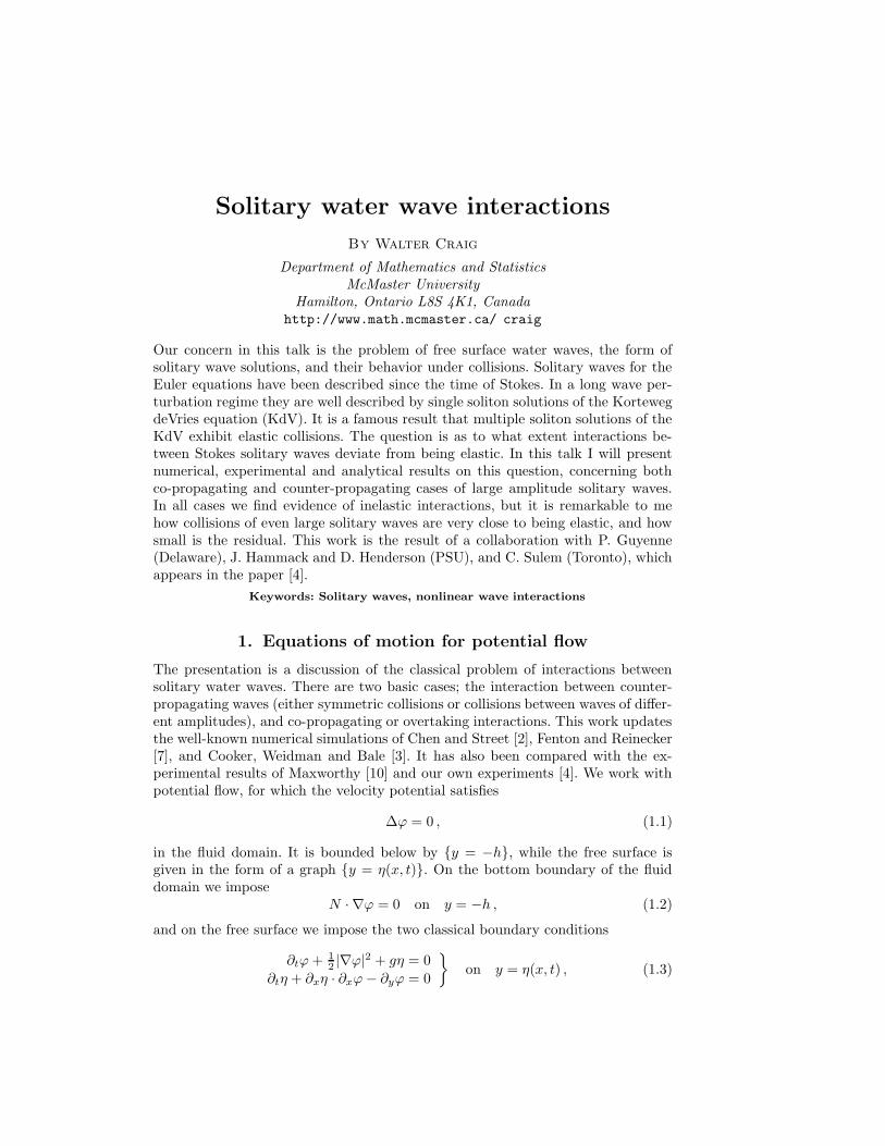
This section is concerned with collisions between two counter-propagating solitarywaves, of nondimensional elevation S1/h and S2/h respectively. The first simula-tions presented here are symmetric head-on collisions between two solitary waves ofequal amplitudes S/h. Features of note are the degree of run-up of the wave crestduring the interaction, given by supx,t |η(x, t)|/h − 2S/h; the phase lag due to themoment’s hesitation of the crests during their interaction; the change in amplitudeof the solitary waves after the interaction, S/h 7→ S+/h; their phase lag a 7→ a+;and the residual waves ηR(x, t) trailing the solitary waves as they exit the collision.We observe that the solitary waves in head-on collisions always lose a small amountof amplitude due to the collision; S+

j < Sj , although this is very small even forinteractions between large solitary waves.

4 W. Craig

020

4060

80100

120140

160

0

10

20

30

40

50

60

70

80

90

0

0.05

0.1

0.15

0.2

x/h

t/(h/g)1/2

η/h

Figure 1. Head-on collision of two solitary waves of equal height S/h = 0.1: The amplitudeafter collision is S+/h = 0.0997 at t/

p

h/g = 90. The phase lag is (aj − a+

j )/h = 0.1370.

020

4060

80100

120140

160

0

10

20

30

40

50

60

70

80

90

0

0.1

0.2

0.3

0.4

0.5

x/h

t/(h/g)1/2

η/h

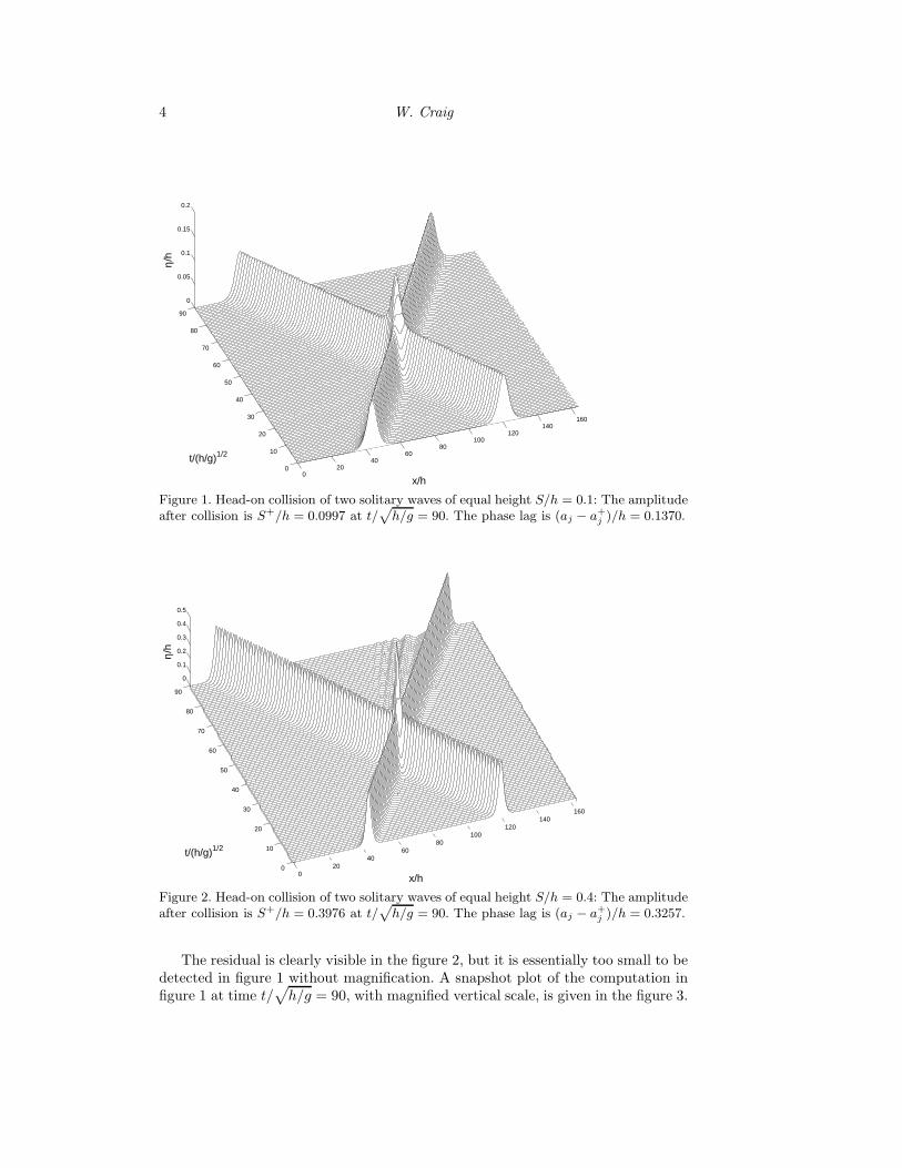
Figure 2. Head-on collision of two solitary waves of equal height S/h = 0.4: The amplitudeafter collision is S+/h = 0.3976 at t/

p

h/g = 90. The phase lag is (aj − a+

j )/h = 0.3257.

The residual is clearly visible in the figure 2, but it is essentially too small to bedetected in figure 1 without magnification. A snapshot plot of the computation infigure 1 at time t/

√

h/g = 90, with magnified vertical scale, is given in the figure 3.

Solitary water wave interactions 5

0 20 40 60 80 100 120 140 160−1

−0.5

0

0.5

1

1.5

2x 10

−3

x/h

η/h

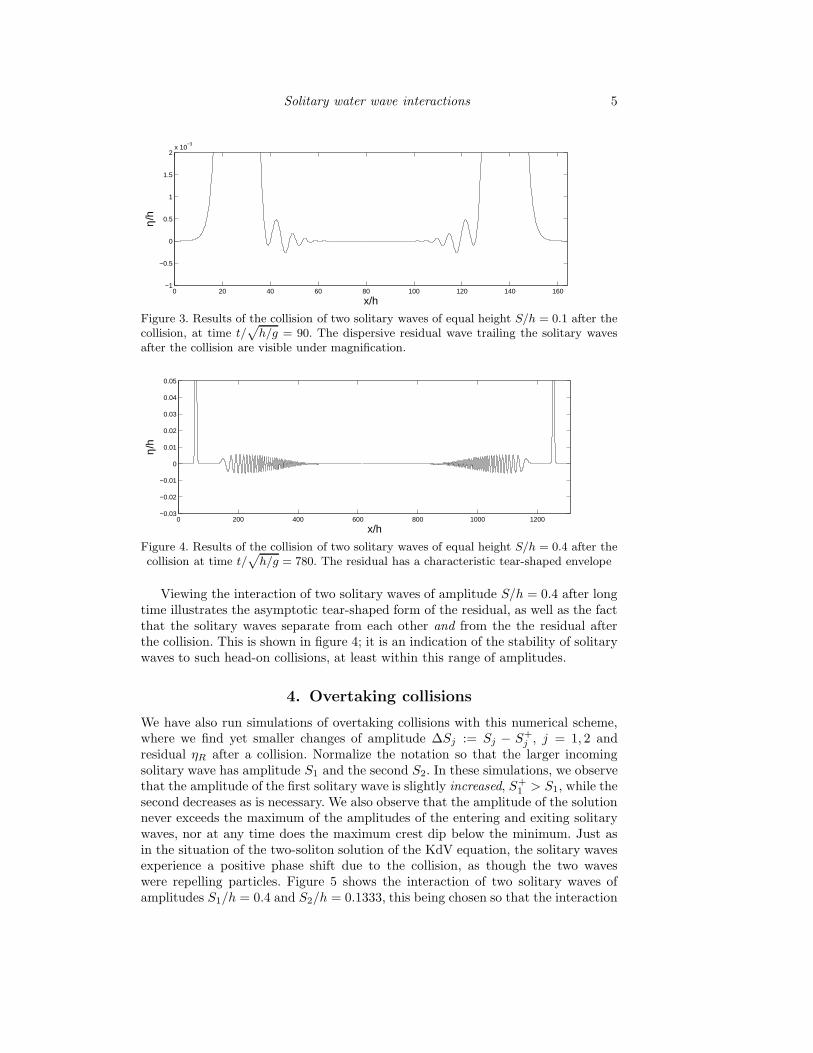
Figure 3. Results of the collision of two solitary waves of equal height S/h = 0.1 after thecollision, at time t/

p

h/g = 90. The dispersive residual wave trailing the solitary wavesafter the collision are visible under magnification.

0 200 400 600 800 1000 1200−0.03

−0.02

−0.01

0

0.01

0.02

0.03

0.04

0.05

x/h

η/h

Figure 4. Results of the collision of two solitary waves of equal height S/h = 0.4 after thecollision at time t/

p

h/g = 780. The residual has a characteristic tear-shaped envelope

Viewing the interaction of two solitary waves of amplitude S/h = 0.4 after longtime illustrates the asymptotic tear-shaped form of the residual, as well as the factthat the solitary waves separate from each other and from the the residual afterthe collision. This is shown in figure 4; it is an indication of the stability of solitarywaves to such head-on collisions, at least within this range of amplitudes.

4. Overtaking collisions

We have also run simulations of overtaking collisions with this numerical scheme,where we find yet smaller changes of amplitude ∆Sj := Sj − S+

j , j = 1, 2 andresidual ηR after a collision. Normalize the notation so that the larger incomingsolitary wave has amplitude S1 and the second S2. In these simulations, we observethat the amplitude of the first solitary wave is slightly increased, S+

1 > S1, while thesecond decreases as is necessary. We also observe that the amplitude of the solutionnever exceeds the maximum of the amplitudes of the entering and exiting solitarywaves, nor at any time does the maximum crest dip below the minimum. Just asin the situation of the two-soliton solution of the KdV equation, the solitary wavesexperience a positive phase shift due to the collision, as though the two waveswere repelling particles. Figure 5 shows the interaction of two solitary waves ofamplitudes S1/h = 0.4 and S2/h = 0.1333, this being chosen so that the interaction

6 W. Craig

020

4060

80100

120140

160

0

100

200

300

400

500

600

700

800

900

1000

0

0.1

0.2

0.3

0.4

0.5

x/h

t/(h/g)1/2

η/h

Figure 5. Overtaking collision of two solitary waves of height S1/h = 0.4, S2/h = 0.1:The amplitudes after collision are S+

1 /h = 0.4003, S+

2 /h = 0.0999 at t/p

h/g = 1000for the large, small wave respectively. The phase shifts are (a+

1 − a1)/h = 2.2974,(a+

2 − a2)/h = 3.6159 respectively.

0 20 40 60 80 100 120 140 160−5

0

5

10x 10

−3

x/h

η/h

Figure 6. Overtaking collision of two solitary waves of height S1/h = 0.4, S2/h = 0.1 att/

p

h/g = 745, which is after the collision. The vertical scale is magnified in order toobserve the dispersive trailing wave generated by the interaction.

is of the Lax category (b) in its form. The simulation is displayed in a frame ofreference in motion at approximately the mean velocity of the two solitary waves.

In figure 6 a view of this simulation with exagerated scale at a time after theinteraction shown clearly the very small but nonzero residual.

5. Energy transfer

Using the conservation laws (1.9)(1.10) and the Hamiltonian (1.4), one can derivea relation between the change in amplitude through a solitary wave interaction

Solitary water wave interactions 7

and the energy that has been transferred to the residual. Using this, it is alsopossible to derive a rigorous upper bound on the energy transfer in terms of theparameters S1/h, S2/h of the initial data. The latter analysis appears in [4]. Toexplain the first relation, an individual solitary wave has mass M(ηS) := m(S),momentum I(ηS , ξS) := µ(S) and energy H(ηS , ξS) := e(S). Our initial data isgiven by two asymptotically separated solitary waves as t 7→ −∞, therefore thetotal mass, momentum and energy of our solution are given by

MT = m(S1) + m(S2)

IT = µ(S1) + µ(S2)

ET = e(S1) + e(S2) . (5.1)

After an interaction has occurred, we will assume that the solution is composed ofthree distinct components; two solitary waves with possibly different amplitudes S+

1

and S+2 , and a residual (ηR(x, t), ξR(x, t)). By conservation, their mass, momenta

and energies satisfy

MT = m(S+1 ) + m(S+

2 ) + mR

IT = µ(S+1 ) + µ(S+

2 ) + µR

ET = e(S+1 ) + e(S+

2 ) + eR . (5.2)

Taking the difference, we find that

(m(S1) − m(S+1 )) + (m(S2) − m(S+

2 )) = mR

(µ(S1) − µ(S+1 )) + (µ(S2) − µ(S+

2 )) = µR

(e(S1) − e(S+1 )) + (e(S2) − e(S+

2 )) = eR . (5.3)

Since the change in amplitude is very small, the difference m(Sj) − m(S+j ) is very

small, j = 1, 2, and the same for µ(Sj) and e(Sj). Approximating by the derivative,we conclude that

m′

1∆S1 + m′

2∆S2 = mR

µ′

1∆S1 + µ′

2∆S2 = µR

e′1∆S1 + e′2∆S2 = eR ; (5.4)

this is now three equations for the two unknowns ∆j , j = 1, 2, whose solution leadsus to an absolute bound on the energy loss due to a collision [4]. Separately fromthis bound, equations (5.4) specify relationships between the mass, momentum andenergy loss to the residual and the change in amplitude ∆Sj from the interaction.

Let us consider the case of symmetric interactions as an example. In this case,µ(S1) = −µ(S2) and therefore IT = 0 and µR = 0. The relation (5.4) then reportsthat

2m′(S) = mR , 2e′(S) = eR . (5.5)

Since in particular e(S) ∼ S3/2 for small S, this predicts that

eR ∼ S1/2∆S . (5.6)

Figure 7 plots the quantity e(S) for a range of simulations ranging from S = 0.025to S = 0.5, verifying its power law behavior. Figure 8 gives our measured values

8 W. Craig

10−2

10−1

100

10−3

10−2

10−1

100

101

S3/2

S/h

HT

Figure 7. Total energy ET vs. wave amplitude S/h: numerical results (circles), power law(S/h)3/2 (solid line).

of ∆S for these simulations, while figure 9 gives the energy eR of the residual.The adherence of thie data to the asymptotic relation (5.6) is quite convincing.The deviation of the lowest two data points from the power law behavior is dueto the long relaxation time of small solutions to their asymptotic values after aninteraction, we believe.

Our data, particularly in figure 8, are at odds with the asymptotic predictions ofC.-H. Su and R. M. Mirie [11], who put forward that ηR = O(S3) while ∆S = o(S3).

The relations (5.4) give a nontrivial result on the mass and energy of the residualand the quantities ∆S+

j in the case of overtaking collisions. From our simulationsand from those in [7], it is observed that ∆S1 < 0. That is, the larger overtaking soli-tary wave gains a (small amount of) amplitude due to the collision, at the expense ofthe smaller one. We note that e(S) is a convex function of S, at least over the rangeof values of S being considered. The implication of (5.4) is that, since eR ≥ 0, it mustbe that |∆S1| < ∆S2; the larger solitary wave cannot gain more amplitude than thesmaller one loses. Using this, a related argument applied to the relation for mass im-plies that mR < 0, because in this case m′(S) is decreasing in S. This fact is seen inthe slight depression left behind two separating solitary waves after their interaction.

Acknowledgements: This research has been supported in part by the Canada Re-search Chairs Program, the NSERC under operating grant #238452, and the NSF undergrant #DMS-0070218. All of the numerical simulations in this note were performed by P.Guyenne.

References

[1] W. J. D. Bateman, C. Swan and P. Taylor. On the efficient numerical simulation ofdirectionally spread surface water waves. J. Comput. Phys. 174, 277 (2001).

Solitary water wave interactions 9

10−2

10−1

100

10−4

10−3

10−2

S3/2

S/h

∆ S

/h

Figure 8. Change in amplitude ∆S/h = (S − S+)/h vs. wave amplitude S/h: numericalresults (circles), power law (S/h)3/2 (solid line).

10−2

10−1

100

10−5

10−4

10−3

10−2

10−1

S2

S/h

HR

Figure 9. Energy of the residual eR vs. nondimensional wave amplitude S/h: numericalresults (circles), power law (S/h)2 (solid line).

[2] R. K.-C. Chan, and R. Street. A computer study of finite amplitude water waves. J.

Comput. Phys. 6, 68 (1970).

[3] M. J. Cooker, P. D. Weidman, and D. S. Bale. Reflection of a high-amplitude solitarywave at a vertical wall. J. Fluid Mech. 342, 141 (1997).

10 W. Craig

[4] W. Craig, P. Guyenne, J. Hammack, D. Henderson and C. Sulem. Solitary wave inter-actions. Physics of Fluids (2005), submitted.

[5] W. Craig & D. Nicholls. Traveling two and three dimensional capillary gravity waves.SIAM: Math. Analysis 32 (2000), pp. 323-359.

[6] W. Craig and C. Sulem. Numerical simulation of gravity waves. J. Comp. Phys.108,pp. 73–83, (1993).

[7] J. D. Fenton, and M. M. Rienecker. A Fourier method for solving nonlinear water-waveproblems: application to solitary-wave interactions. J. Fluid Mech. 118, 411 (1982).

[8] J. Hadamard. Lecons sur le calcul des variations. Hermann, Paris, 1910; paragraph§249.

[9] J. Hadamard. Sur les ondes liquides. Rend. Acad. Lincei 5, (1916) no. 25, pp. 716–719.

[10] T. Maxworthy. Experiments on the collision between two solitary waves. J. Fluid

Mech. 76, 177 (1976).

[11] C. H. Su, and R. M. Mirie. On head-on collisions between two solitary waves. J. Fluid

Mech. 98, 509 (1980).

[12] M. Tanaka. The stability of solitary waves. Phys. Fluids 29, 650 (1986).

[13] V.E. Zakharov. Stability of periodic waves of finite amplitude on the surface of a deepfluid. J. Appl. Mech. Tech. Phys. 9 (1968), pp. 190–194.