NREL is a national laboratory of the U.S. Department of Energy, Office of Energy Efficiency & Renewable Energy, operated by the Alliance for Sustainable Energy, LLC.

Contract No. DE-AC36-08GO28308

SolTrace: A Ray-Tracing Code for Complex Solar Optical Systems Tim Wendelin and Aron Dobos National Renewable Energy Laboratory

Allan Lewandowski Allan Lewandowski Solar Consulting LLC

Technical Report NREL/TP-5500-59163 October 2013

NREL is a national laboratory of the U.S. Department of Energy, Office of Energy Efficiency & Renewable Energy, operated by the Alliance for Sustainable Energy, LLC.

National Renewable Energy Laboratory 15013 Denver West Parkway Golden, Colorado 80401 303-275-3000 • www.nrel.gov

Contract No. DE-AC36-08GO28308

SolTrace: A Ray-Tracing Code for Complex Solar Optical Systems Tim Wendelin and Aron Dobos National Renewable Energy Laboratory

Allan Lewandowski Allan Lewandowski Solar Consulting LLC

Prepared under Task No. ST11.3070

Technical Report NREL/TP-5500-59163 October 2013

NOTICE

This report was prepared as an account of work sponsored by an agency of the United States government. Neither the United States government nor any agency thereof, nor any of their employees, makes any warranty, express or implied, or assumes any legal liability or responsibility for the accuracy, completeness, or usefulness of any information, apparatus, product, or process disclosed, or represents that its use would not infringe privately owned rights. Reference herein to any specific commercial product, process, or service by trade name, trademark, manufacturer, or otherwise does not necessarily constitute or imply its endorsement, recommendation, or favoring by the United States government or any agency thereof. The views and opinions of authors expressed herein do not necessarily state or reflect those of the United States government or any agency thereof.

Available electronically at http://www.osti.gov/bridge

Available for a processing fee to U.S. Department of Energy and its contractors, in paper, from:

U.S. Department of Energy Office of Scientific and Technical Information P.O. Box 62 Oak Ridge, TN 37831-0062 phone: 865.576.8401 fax: 865.576.5728 email: mailto:reports@adonis.osti.gov

Available for sale to the public, in paper, from:

U.S. Department of Commerce National Technical Information Service 5285 Port Royal Road Springfield, VA 22161 phone: 800.553.6847 fax: 703.605.6900 email: orders@ntis.fedworld.gov online ordering: http://www.ntis.gov/help/ordermethods.aspx

Cover Photos: (left to right) PIX 16416, PIX 17423, PIX 16560, PIX 17613, PIX 17436, PIX 17721

Printed on paper containing at least 50% wastepaper, including 10% post consumer waste.

iv This report is available at no cost from the National Renewable Energy Laboratory (NREL) at www.nrel.gov/publications.

Executive Summary SolTrace is an optical simulation tool designed to model optical systems used in concentrating solar power (CSP) applications. The code was first written in early 2003, but has seen significant modifications and changes since its inception, including conversion from a Pascal-based software development platform to C++. SolTrace is unique in that it can model virtually any optical system utilizing the sun as the source. It has been made available for free and as such is in use worldwide by industry, universities, and research laboratories. The fundamental design of the code is discussed, including enhancements and improvements over the earlier version. Comparisons are made with other optical modeling tools, both non-commercial and commercial in nature. Finally, modeled results are shown for some typical CSP systems and, in one case, compared to measured optical data.

v This report is available at no cost from the National Renewable Energy Laboratory (NREL) at www.nrel.gov/publications.

Table of Contents 1 Introduction ........................................................................................................................................... 1

1.1 Ray-Tracing Methodology ............................................................................................................ 2 2 Sun Definition ....................................................................................................................................... 4 3 Optical Element Definition ................................................................................................................... 6 4 Using SolTrace ...................................................................................................................................... 9 5 NREL High Flux Solar Furnace ......................................................................................................... 10 6 Modeling Measured Optics ................................................................................................................ 12 7 Conclusions ........................................................................................................................................ 13 References ................................................................................................................................................. 14

1 This report is available at no cost from the National Renewable Energy Laboratory (NREL) at www.nrel.gov/publications.

1 Introduction Designing and building efficient, cost-effective concentrating solar power (CSP) systems requires highly specialized resources. In particular, understanding the solar resource and how best to convert that resource into usable energy requires specialized modeling tools to predict system and economic performance. One of the most important aspects of the overall system is the optical design. Because optical systems for CSP applications can be highly complex with many parameters to optimize, it is not practical to physically build and test the many possible preliminary prototypes as part of the product development path. Instead, computer codes are used to model these systems and predict the optical behavior and performance. Design optimization can be accomplished much more efficiently this way, resulting in fewer prototypes and a shorter development path. These programs can be coupled with other tools such as structural and systems analysis codes to achieve the desired performance and economic goals.

One such optical analysis tool is SolTrace, which began its development at the National Renewable Energy Laboratory (NREL) in early 2003 [1] and is available for download at www.nrel.gov/csp/soltrace/. At that time, optical design tools existed that were specific to certain CSP technologies, e.g., parabolic dish and central receiver [2], [3], [4], [5], but a design tool was needed that could model the significant variety of new solar optical systems being considered for power generation, materials processing, process heating, etc. Commercial optical modeling packages existed that could have been used for such geometries, but these tools were created for more fundamental optical problems such as lens design, not for efficiently modeling solar optical systems using the sun as the source. Given these gaps in the available toolset, NREL decided to develop a program that would build on the methodology behind earlier codes specific to certain geometries, but extend the geometry set to virtually any combination of these geometries. This was the original inception of the SolTrace tool; since that time, significant changes and enhancements have been made to keep the tool state of the art and relevant. These include code conversion from Pascal to C++, multi-processor utilization, new input options, and more detailed optical interaction algorithms.

SolTrace is one of several options available for modeling CSP systems. Since its inception, similar tools have been developed by others in the CSP community, such as Tonatiuh [1]. In addition, commercial ray-tracing packages also exist such as ASAP by Breault Research, but these are intended for more general optical system design and, as such, are not “solar friendly.” While they can be used, they require significant effort to learn and model the complex solar designs using the sun as the source. The remainder of this paper discusses the methodology behind SolTrace, some primary capabilities of the code, and some modeling results illustrating the types of systems that can be modeled with SolTrace.

2 This report is available at no cost from the National Renewable Energy Laboratory (NREL) at www.nrel.gov/publications.

1.1 Ray-Tracing Methodology The code utilizes a ray-tracing methodology outlined in [6]. A specified number of rays are traced from the sun through the system, and each traces through the defined system while encountering various optical interactions. Some of these interactions are probabilistic in nature (e.g., selection of sun angle from sun angular intensity distribution) while others are deterministic (e.g., calculation of ray intersection with an analytically described surface and resultant redirection). Such a code has the advantage over codes based on convolution of moments in that it replicates real photon interactions and can therefore provide accurate results for complex systems that cannot be modeled otherwise. The disadvantage is longer processing time. Accuracy increases with the number of rays traced, and larger ray numbers means more processing time. Complex geometries also translate into longer run times. However, the required number of rays is also a function of the desired result. For example, fewer rays (and therefore less time) are needed to determine relative changes in optical efficiency for different sun angles on a given solar concentrator than are typically needed to accurately assess the flux distribution on the receiver of that same concentrator.

An optical system is organized into “stages” within a global coordinate system. A stage is loosely defined as a section of the optical geometry that, once a ray exits the stage, will not be re-entered by the ray on the remainder of its path through the system. A complete system geometry may consist of one or more stages. It is incumbent on the user to define the stage geometry accordingly. The motivation behind the stage concept is to employ efficient tracing and therefore save processing time and allow for a modular representation of a system. The other benefit of stages is that they can also be saved and employed in other system geometries without the need for recalculating element positions and orientations. Segmentation of the geometry via stages may also be useful in assignment of different coordinate systems for specific geometries and can make adjustment of locations far more straightforward.

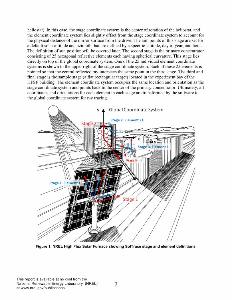
A stage is comprised of “elements.” Each element consists of a surface, an optical interaction type, an aperture shape, and, if appropriate, a set of optical properties. The location and orientation of stages are defined within the global coordinate system, whereas the location and orientation of elements are specified within the coordinate system of the particular stage in which they are defined. Stages can be one of two types: optical or virtual. An optical stage is defined as one that physically interacts with the rays. Conversely, a virtual stage is defined as one that does not physically interact with the rays. The virtual stage is useful for determining ray locations and directions and incident power or flux at various positions along the optical path without physically affecting ray trajectory. Elements defined within a virtual stage therefore have no optical properties because they do not interact with the rays. Optical stages consist of elements that interact with the rays, potentially altering their trajectories. These elements have optical properties and interaction types associated with them. Beyond this, optical and virtual stages are identical in how they are defined and used. Stages can be duplicated and moved around as groups of elements and saved for use in other system geometries. The NREL High Flux Solar Furnace (HFSF) [7] is shown as an example of a multi-stage, multi-element system in Figure 1. Note the global (black), stage (red), and element (blue) coordinate systems. In this example, there are a total of three stages, and the global coordinate system is located at the center of the second stage. This arrangement was chosen because the primary concentrator of the system is the second stage. The first stage is comprised of one flat rectangular reflective element (the

3 This report is available at no cost from the National Renewable Energy Laboratory (NREL) at www.nrel.gov/publications.

heliostat). In this case, the stage coordinate system is the center of rotation of the heliostat, and the element coordinate system lies slightly offset from the stage coordinate system to account for the physical distance of the mirror surface from the drive. The aim points of this stage are set for a default solar altitude and azimuth that are defined by a specific latitude, day of year, and hour. The definition of sun position will be covered later. The second stage is the primary concentrator consisting of 25 hexagonal reflective elements each having spherical curvature. This stage lies directly on top of the global coordinate system. One of the 25 individual element coordinate systems is shown to the upper right of the stage coordinate system. Each of these 25 elements is pointed so that the central reflected ray intersects the same point in the third stage. The third and final stage is the sample stage (a flat rectangular target) located in the experiment bay of the HFSF building. The element coordinate system occupies the same location and orientation as the stage coordinate system and points back to the center of the primary concentrator. Ultimately, all coordinates and orientations for each element in each stage are transformed by the software to the global coordinate system for ray tracing.

Figure 1. NREL High Flux Solar Furnace showing SolTrace stage and element definitions.

4 This report is available at no cost from the National Renewable Energy Laboratory (NREL) at www.nrel.gov/publications.

2 Sun Definition Two characteristics completely define the “sun” as the light source: the angular intensity distribution of light across the sun’s disk, referred to as the sun shape, and the sun’s position. There are two options for defining the sun position. One option is to define a point in the global coordinate system such that a vector from this point to the global coordinate system origin defines the sun direction. In this case the user must place that point above the elements in the initial stage, and the relationship between the coordinate system and the earth is not constrained. The other option is to define a particular site latitude and time (day of year and local solar hour.) From this information, the sun direction is determined assuming the z-axis of the global coordinate system points due north, the y-axis points towards zenith, and the x-axis points due west. SolTrace calculates the sun position in azimuth and elevation and determines a corresponding unit vector, Equation 5, based on Equations 1–4 given latitude L (+north, -south), Julian day of year D, and hour of day H in local solar time [8]. In the case where the element geometry depends on sun position (e.g., for a heliostat in a tower geometry), the user must use these same equations to determine element aim points. These equations are based on solar time and come from the spherical geometric relationship of the earth and sun, and they do not account for longitude, eccentricity of the earth’s orbit, or impacts due to atmospheric effects.

𝛿 = 𝑎𝑟𝑐𝑠𝑖𝑛(0.39795𝑐𝑜𝑠(0.98563(𝐷 − 173))) (1)

𝜔 = 15(𝐻 − 12) (2)

𝛼 = 𝑎𝑟𝑐𝑠𝑖𝑛(𝑠𝑖𝑛𝛿𝑠𝑖𝑛𝐿 + 𝑐𝑜𝑠𝛿𝑐𝑜𝑠𝜔𝑐𝑜𝑠𝐿) (3)

𝛾 = 𝑎𝑟𝑐𝑐𝑜𝑠 �𝑠𝑖𝑛𝛿𝑐𝑜𝑠𝐿 – 𝑐𝑜𝑠𝛿𝑠𝑖𝑛𝐿𝑐𝑜𝑠𝜔𝑐𝑜𝑠𝛼

� (4)

𝑥 = − 𝑠𝑖𝑛 𝛾 𝑐𝑜𝑠 𝛼

𝑦 = 𝑠𝑖𝑛 𝛼

𝑧 = 𝑐𝑜𝑠 𝛾 𝑐𝑜𝑠 𝛼 (5)

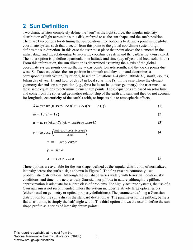
Three options are available for the sun shape, defined as the angular distribution of normalized intensity across the sun’s disk, as shown in Figure 2. The first two are commonly used probabilistic distributions. Although the sun shape varies widely with terrestrial location, sky conditions, and time, it is neither truly Gaussian nor pillbox in nature, although the pillbox approximation is adequate for a large class of problems. For highly accurate systems, the use of a Gaussian sun is not recommended unless the system includes relatively large optical errors (either based on geometry or optical property definitions). The parameter defining a Gaussian distribution for the sun’s disk is the standard deviation, σ. The parameter for the pillbox, being a flat distribution, is simply the half-angle width. The third option allows the user to define the sun shape profile as a series of intensity datum points.

5 This report is available at no cost from the National Renewable Energy Laboratory (NREL) at www.nrel.gov/publications.

Figure 2. Gaussian, pillbox, and user-defined measured sun shapes.

6 This report is available at no cost from the National Renewable Energy Laboratory (NREL) at www.nrel.gov/publications.

3 Optical Element Definition Only the first stage of an optical system “sees” the sun. That is, rays are traced from the sun only to the first stage, omitting other stages regardless of their spatial arrangement. Subsequent stages only “see” the rays that come from the previous stage. It is important to know this for shading purposes. In general, if it is possible and reasonable to define all optical elements in the first stage, then it is most accurate to do so. Individual optical elements within a stage can have either reflective or refractive optical properties. Sets of optical properties can be defined within a SolTrace project, and each optical element is associated with one of these property sets. For refractive optics, the transmissivity and the real component of the refraction indices are relevant and used at this time. An element at its core is a single surface or interface.

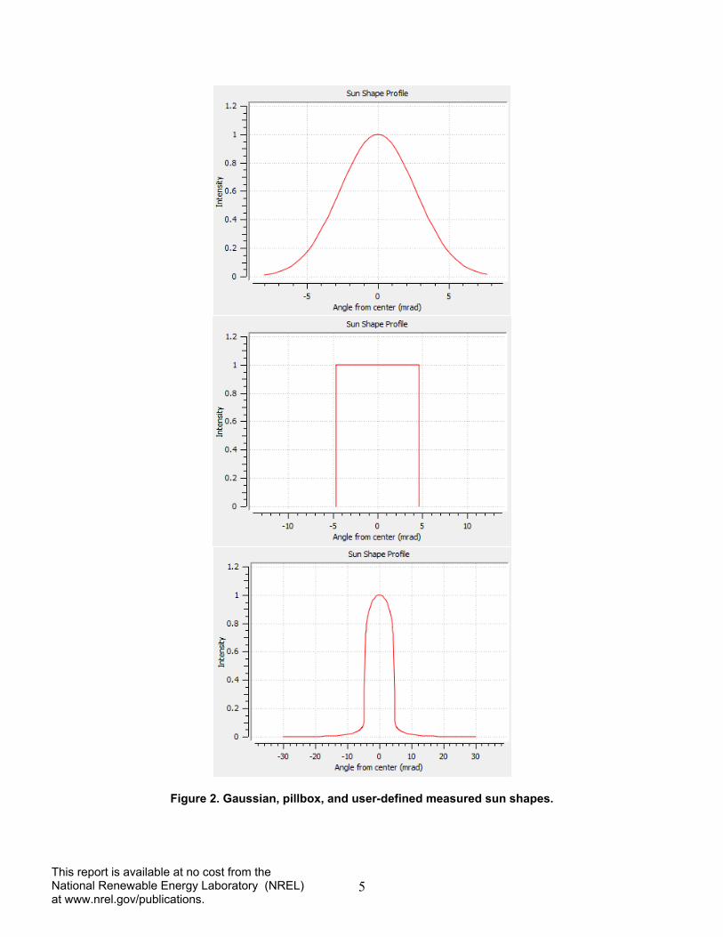
A real physical refractive component is actually constructed from two elements (or surfaces). In Figure 3, for example, a sheet of glass consists of two surfaces (or elements) separated by the glass media between. A ray passes from one surface to the glass media, is refracted, and then passes through the other surface back to the air. The first element would be defined with the index of refraction of air on the front side and the index of refraction of glass on the back side. The second surface would be defined with the index of refraction of glass on the front side and the index of refraction of air on the back side. The front and back surfaces are dependent on how the element geometry is defined. Surfaces other than flat would construct lenses. The transmissivity is the fraction of rays (0 to 1.0) that pass through an element. So, if in this example the glass sheet transmits 98%, then one of the elements should be defined with a transmissivity of 0.98 and the other 1.0, or both could be defined with transmissivities of 0.99 (the product of the two transmissivity values should equal the overall value desired). This choice is arbitrary. Care should be taken when defining the element to keep track of the element aim point direction to properly assign index of refraction to the correct side (front or back) and to be consistent with the index for the intermediate material.

Figure 3. Elements/surfaces are combined to model a refractive sheet of glass.

7 This report is available at no cost from the National Renewable Energy Laboratory (NREL) at www.nrel.gov/publications.

SolTrace calculates reflection and refraction at surface interfaces using the well-known Fresnel equations. As a result, characteristics of refractive surfaces like total internal reflection (TIR) are managed correctly. At any given ray intersection with a refractive surface, SolTrace first determines the side (front or back) and uses the associated optical properties for further interactions at that intersection. First, whether a ray is absorbed is determined by comparing a random number to the transmittance value from the optical properties. If the ray is absorbed, SolTrace moves on to the next ray. If the ray is not absorbed, then the reflection factors for both parallel and perpendicular polarization are calculated. These are based on the ideal surface slope plus any slope errors associated with the surface (either front or back). The two values are averaged to determine the possible reflected fraction. The possible transmitted fraction is just 1-ρ, where ρ is the surface reflectance. A random number (0–1) is generated to determine whether the ray is reflected or transmitted. If the calculated reflectance is less than this random number, the ray is reflected at the specular angle (θ1 in Figure 3). If greater, the ray is transmitted. If the random number is less than this value, the ray is transmitted and propagated into the medium at the calculated angle (θ2 in Figure 3). Currently, a more correct method of determining absorption based on material properties and path length is not used, and the user is cautioned to utilize the optical properties appropriately (in particular the selection of reflective or refractive optical properties for elements depending on whether a ray has entered a refractive medium).

For reflective optics, one element (or surface) is sufficient to model a mirror because transmission is allowed. The relevant parameter is the reflectivity, and the element still possesses both back- and front-side values. For example, a mirror could have rays that intersect the back side (e.g., a heliostat in a field); the back should then be assigned a reflectance of zero. A recently added feature of SolTrace is the reflectance ρ as a function of incidence angle.

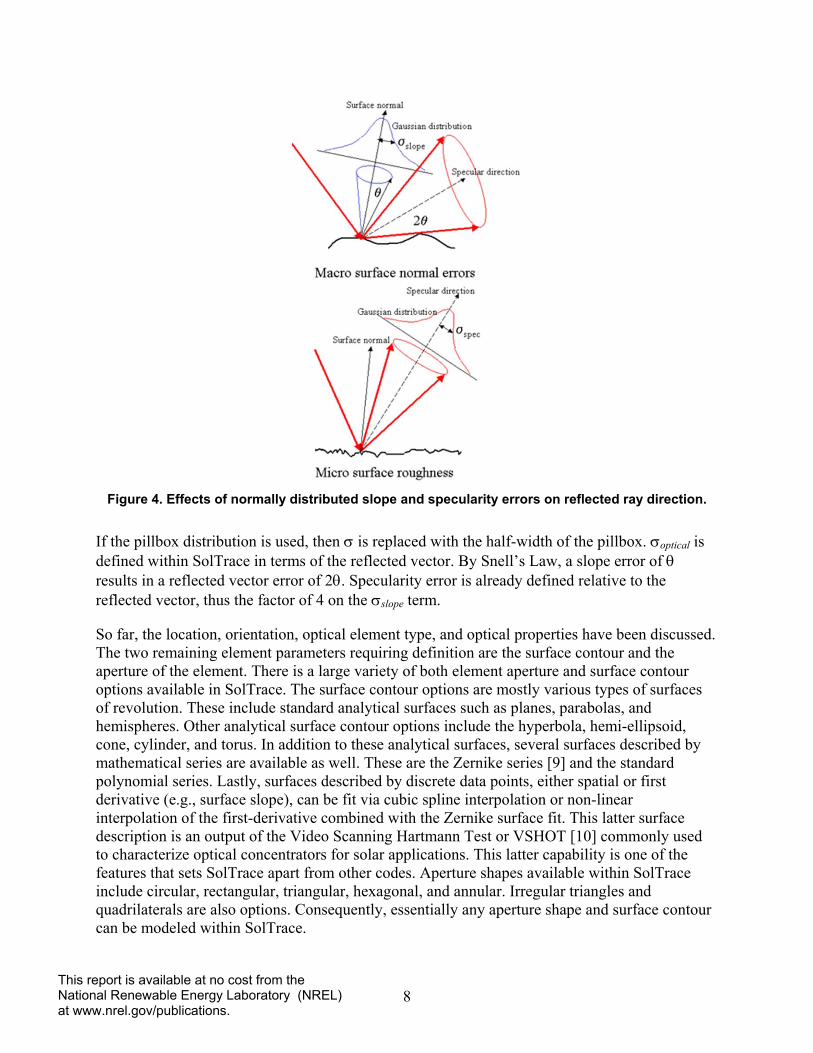
For both refractive and reflective optics, another set of parameters applies that defines the optical accuracy of the surface. In addition to the effects of the element surface shape on ray direction, two random errors can be included that affect ray interaction at the surface of an element: slope error and surface specularity. Surface slope error is a macro feature while specularity is a micro structure effect. Both are illustrated in Figure 4 for the case of a reflective surface with Gaussian error distribution having a standard deviation of σ. The total error is given by Equation 6.

𝜎𝑜𝑝𝑡𝑖𝑐𝑎𝑙 = �4𝜎𝑠𝑙𝑜𝑝𝑒 2 + 𝜎𝑠𝑝𝑒𝑐𝑢𝑙𝑎𝑟𝑖𝑡𝑦2 �1/2

(6)

8 This report is available at no cost from the National Renewable Energy Laboratory (NREL) at www.nrel.gov/publications.

Figure 4. Effects of normally distributed slope and specularity errors on reflected ray direction.

If the pillbox distribution is used, then σ is replaced with the half-width of the pillbox. σoptical is defined within SolTrace in terms of the reflected vector. By Snell’s Law, a slope error of θ results in a reflected vector error of 2θ. Specularity error is already defined relative to the reflected vector, thus the factor of 4 on the σslope term.

So far, the location, orientation, optical element type, and optical properties have been discussed. The two remaining element parameters requiring definition are the surface contour and the aperture of the element. There is a large variety of both element aperture and surface contour options available in SolTrace. The surface contour options are mostly various types of surfaces of revolution. These include standard analytical surfaces such as planes, parabolas, and hemispheres. Other analytical surface contour options include the hyperbola, hemi-ellipsoid, cone, cylinder, and torus. In addition to these analytical surfaces, several surfaces described by mathematical series are available as well. These are the Zernike series [9] and the standard polynomial series. Lastly, surfaces described by discrete data points, either spatial or first derivative (e.g., surface slope), can be fit via cubic spline interpolation or non-linear interpolation of the first-derivative combined with the Zernike surface fit. This latter surface description is an output of the Video Scanning Hartmann Test or VSHOT [10] commonly used to characterize optical concentrators for solar applications. This latter capability is one of the features that sets SolTrace apart from other codes. Aperture shapes available within SolTrace include circular, rectangular, triangular, hexagonal, and annular. Irregular triangles and quadrilaterals are also options. Consequently, essentially any aperture shape and surface contour can be modeled within SolTrace.

9 This report is available at no cost from the National Renewable Energy Laboratory (NREL) at www.nrel.gov/publications.

4 Using SolTrace The first step in defining a SolTrace project is to define the sun shape and direction. Next, sets of optical properties are created that will ultimately be associated with the optical elements in the system. Finally, the optical system geometry is created, including stage definitions and element definitions within those stages. It is here where each element is connected with one of the optical property sets defined earlier. Once the system is totally defined, it can be saved to a file for later analysis.

All data comprising stage and element definition (e.g., location, orientation, aperture shape, surface contour, optical properties, etc.) are entered alphanumerically via forms. A common practice is to use a spreadsheet program to calculate this data and copy the data into the SolTrace input form. Another recently implemented feature of SolTrace is the ability to define geometry using a free three-dimensional (3D) modeling tool called Trimble SketchUp (formerly Google SketchUp). A SolTrace plug-in created for SketchUp allows SolTrace element and stage data to be generated from the 3D modeling tool and imported directly into SolTrace.

Once the system is defined, it can be traced. The user can select any number of rays to be traced through the system. This value depends on the detail needed in the results. For example, optical efficiency information can be obtained with fewer rays than needed for a detailed flux map. In general, ray numbers on the order of one million are required for flux mapping. Once the system has been traced, the results can be viewed in a number of ways. Three-dimensional scatter plots of ray intersections with various elements can be viewed, with or without the path of the rays shown. Flux maps on planar or cylindrical elements can also be generated. Statistical information, such as centroids, peak flux, peak flux uncertainty, average flux, etc., is calculated and supplied with the graphics. All the data generated by SolTrace, ray intersection locations, and directions at various elements, can be saved to a file for reporting and/or post-processing with other software.

Another powerful feature of SolTrace is its scripting capability. SolTrace uses a fast and powerful script engine that allows automation of SolTrace to run multiple sun definitions, optical geometries, and/or optical properties without the need for user interaction. One possible use of scripting could be to model a solar power tower at different sun positions over the course of a whole year. The script would take care of calculating all of the heliostat orientations at each time step, running the ray-trace simulation, saving results, and generating the desired output data and statistics.

10 This report is available at no cost from the National Renewable Energy Laboratory (NREL) at www.nrel.gov/publications.

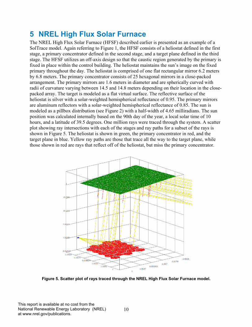
5 NREL High Flux Solar Furnace The NREL High Flux Solar Furnace (HFSF) described earlier is presented as an example of a SolTrace model. Again referring to Figure 1, the HFSF consists of a heliostat defined in the first stage, a primary concentrator defined in the second stage, and a target plane defined in the third stage. The HFSF utilizes an off-axis design so that the caustic region generated by the primary is fixed in place within the control building. The heliostat maintains the sun’s image on the fixed primary throughout the day. The heliostat is comprised of one flat rectangular mirror 6.2 meters by 6.8 meters. The primary concentrator consists of 25 hexagonal mirrors in a close-packed arrangement. The primary mirrors are 1.6 meters in diameter and are spherically curved with radii of curvature varying between 14.5 and 14.8 meters depending on their location in the close-packed array. The target is modeled as a flat virtual surface. The reflective surface of the heliostat is silver with a solar-weighted hemispherical reflectance of 0.95. The primary mirrors are aluminum reflectors with a solar-weighted hemispherical reflectance of 0.85. The sun is modeled as a pillbox distribution (see Figure 2) with a half-width of 4.65 milliradians. The sun position was calculated internally based on the 90th day of the year, a local solar time of 10 hours, and a latitude of 39.5 degrees. One million rays were traced through the system. A scatter plot showing ray intersections with each of the stages and ray paths for a subset of the rays is shown in Figure 5. The heliostat is shown in green, the primary concentrator in red, and the target plane in blue. Yellow ray paths are those that trace all the way to the target plane, while those shown in red are rays that reflect off of the heliostat, but miss the primary concentrator.

Figure 5. Scatter plot of rays traced through the NREL High Flux Solar Furnace model.

11 This report is available at no cost from the National Renewable Energy Laboratory (NREL) at www.nrel.gov/publications.

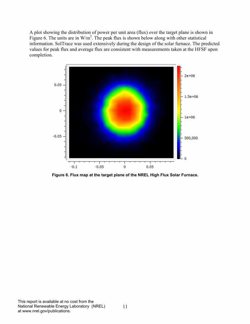
A plot showing the distribution of power per unit area (flux) over the target plane is shown in Figure 6. The units are in W/m2. The peak flux is shown below along with other statistical information. SolTrace was used extensively during the design of the solar furnace. The predicted values for peak flux and average flux are consistent with measurements taken at the HFSF upon completion.

Figure 6. Flux map at the target plane of the NREL High Flux Solar Furnace.

12 This report is available at no cost from the National Renewable Energy Laboratory (NREL) at www.nrel.gov/publications.

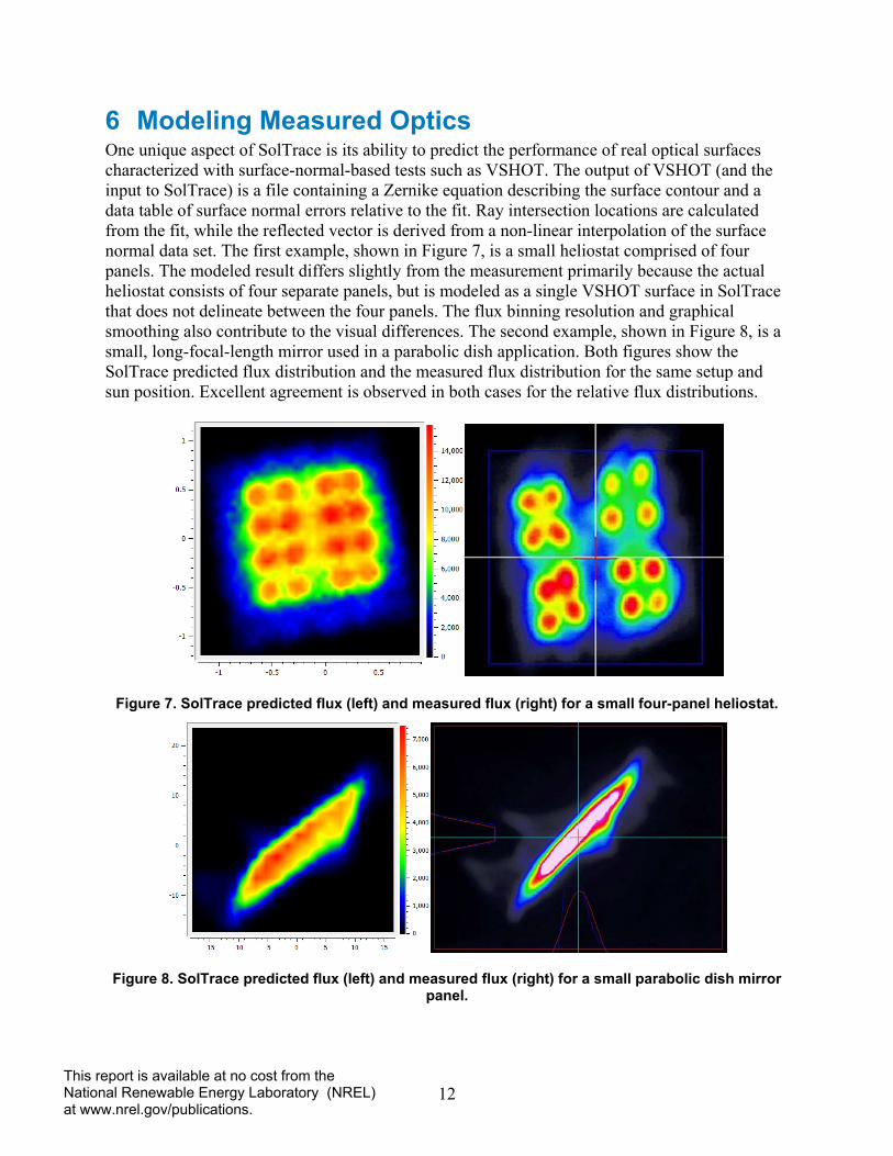
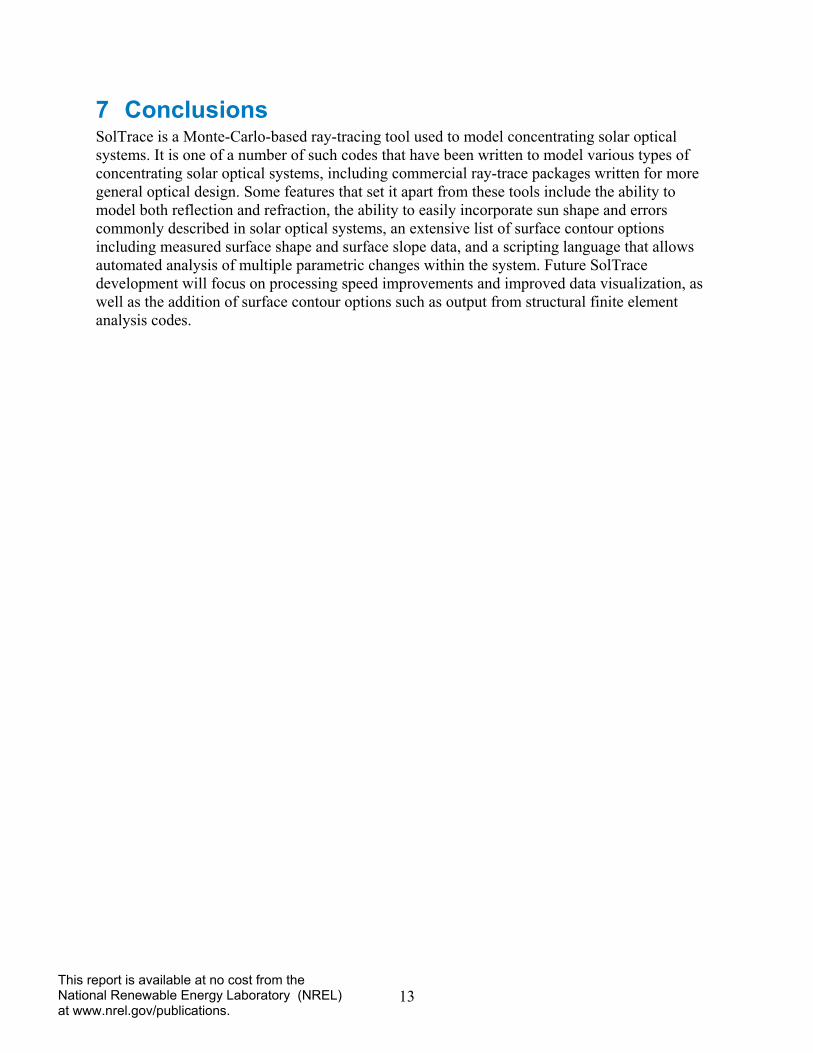
6 Modeling Measured Optics One unique aspect of SolTrace is its ability to predict the performance of real optical surfaces characterized with surface-normal-based tests such as VSHOT. The output of VSHOT (and the input to SolTrace) is a file containing a Zernike equation describing the surface contour and a data table of surface normal errors relative to the fit. Ray intersection locations are calculated from the fit, while the reflected vector is derived from a non-linear interpolation of the surface normal data set. The first example, shown in Figure 7, is a small heliostat comprised of four panels. The modeled result differs slightly from the measurement primarily because the actual heliostat consists of four separate panels, but is modeled as a single VSHOT surface in SolTrace that does not delineate between the four panels. The flux binning resolution and graphical smoothing also contribute to the visual differences. The second example, shown in Figure 8, is a small, long-focal-length mirror used in a parabolic dish application. Both figures show the SolTrace predicted flux distribution and the measured flux distribution for the same setup and sun position. Excellent agreement is observed in both cases for the relative flux distributions.

Figure 7. SolTrace predicted flux (left) and measured flux (right) for a small four-panel heliostat.

Figure 8. SolTrace predicted flux (left) and measured flux (right) for a small parabolic dish mirror panel.

13 This report is available at no cost from the National Renewable Energy Laboratory (NREL) at www.nrel.gov/publications.

7 Conclusions SolTrace is a Monte-Carlo-based ray-tracing tool used to model concentrating solar optical systems. It is one of a number of such codes that have been written to model various types of concentrating solar optical systems, including commercial ray-trace packages written for more general optical design. Some features that set it apart from these tools include the ability to model both reflection and refraction, the ability to easily incorporate sun shape and errors commonly described in solar optical systems, an extensive list of surface contour options including measured surface shape and surface slope data, and a scripting language that allows automated analysis of multiple parametric changes within the system. Future SolTrace development will focus on processing speed improvements and improved data visualization, as well as the addition of surface contour options such as output from structural finite element analysis codes.

14 This report is available at no cost from the National Renewable Energy Laboratory (NREL) at www.nrel.gov/publications.

References [1] Wendelin, T. “SolTrace: A New Optical Modeling Tool For Concentrating Solar Optics.”

International Solar Energy Conference, 2003; pp. 15–18.

[2] Dellin, T. An improved Hermite expansion calculation of the flux distribution from heliostats. SAND79-8619. Albuquerque, NM: Sandia National Laboratories, 1979.

[3] Kistler, B.L. “A Users Manual for DELSOL3: A Computer Code for Calculating the Optical Performance and Optimal System Design for Solar Thermal Central Receiver Plants.” Proc. J. Energy, 1986.

[4] Lipps, F. “A cellwise method for the optimization of large central receiver systems.” Solar Energy 20(6), 1978; pp. 505–516.

[5] Ratzel, A.C.; Boughton. B.D. CIRCE.001: A Computer Code for Analysis of Point Focus Concentrators with Flat Targets. SAND86-1966. Albuquerque, NM: Sandia National Laboratories, 1987.

[6] Spencer, G.; Murty, M. “General ray-tracing procedure.” JOSA 52(6), 1962; pp. 672–676.

[7] Lewandowski, A. “The design of an ultra-high flux solar test capability.” Proc. 24th Intersociety Energy Conversion Engr. Conf., 1989; pp. 1979–1983.

[8] Duffie, J.A.; Beckman, W.A. Solar Engineering of Thermal Processes. 3rd ed. New York: John Wiley and Sons, Inc., 2006.

[9] Malacara, D. Optical Shop Testing. New York: John Wiley and Sons, Inc., 1978.

[10] Jones, S.A.; Gruetzner, J.K.; Houser, R.M.; Edgar, R.M.; Wendelin, T.J. “VSHOT measurement uncertainty and experimental sensitivity study.” Proc. 32nd Intersociety Energy Conversion Engr. Conf. No. 97CH6203, 1997; pp. 1877–1882.

[11] Blanco, M.J.; Amieva, J.M.; Mancillas, A. “The Tonatiuh Software Development Project: An Open Source Approach to the Simulation of Solar Concentrating Systems.” Proc. ASME Computers and Information in Engr., 2005; pp. 157–164.

[12] Stine, B.W.; Harrigan, R.W. Solar Energy Fundamentals and Design. New York: John Wiley and Sons, Inc., 1985.

[13] Walzel, M.D.; Lipps, F.W.; Vant-Hull, L.L. “A solar flux density calculation for a solar tower concentrator using a two-dimensional Hermite function expansion.” Solar Energy 19, 1977; pp. 239–256.