Solution Algorithms for Viscous Flow

Antony JamesonDepartment of Aeronautics and Astronautics

Stanford University, Stanford CA

Indian Institute of ScienceBangalore, India

September 20, 2004

2

Flo3xx

Computational Aerodynamics onArbitrary Meshes

Antony JamesonGeorg May

3

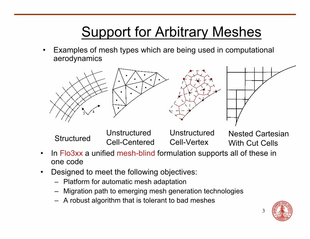
Support for Arbitrary Meshes

• In Flo3xx a unified mesh-blind formulation supports all of these inone code

• Designed to meet the following objectives:– Platform for automatic mesh adaptation– Migration path to emerging mesh generation technologies– A robust algorithm that is tolerant to bad meshes

• Examples of mesh types which are being used in computationalaerodynamics

StructuredNested CartesianWith Cut Cells

UnstructuredCell-Centered

UnstructuredCell-Vertex

4

Support for Arbitrary Meshes

• Conservation laws are enforced on discrete control volumes

• Fluxes of conserved variables are exchanged through interfaces betweenthese cells

• Independent of the mesh topology, eachinterface separates exactly two control volumes(on the right, face N separates cells A and B)

All algorithms are expressed in terms of ageneric interface-based data structure

5

Treatment of Structured Meshes

• Associate first and second neighbors with each face

• Allows implementation of standard schemes with five-point stencils(Jameson-Schmidt-Turkel JST, SLIP) in the same code

• Eliminates the need for gradient reconstruction

• Numerical experiments verify 25% overhead due to indirect addressing incomparison with standard structured-code implementation (FLO107)

Second Neighbors

First Neighbors

Interface Flux

6

Flo3xx in Action…

• From IGES definition to completed result in one week, including CAD fixes, meshgeneration

• We need to be able to compute extreme test cases• This concerns both complexity of geometry and flow conditions

Geometry Courtesy of Lockheed Skunk Works

Mach Number - Upper

Lockheed SR71 at M= 3.2, - Euler calculation with 1.5 Million grid points

0

0.1

0.2

0.3

0.4

0.5

0.6

0 2 4 6 8 10 12 14 16 18 20

Angle of Attack w.r.t Fuselage (deg)

CL

FLO-XX, Mach3.25FLO-XX, Mach2.50Manual, Mach 3.25

Manual, Mach 2.50

Angle-of-Attack sweep

7

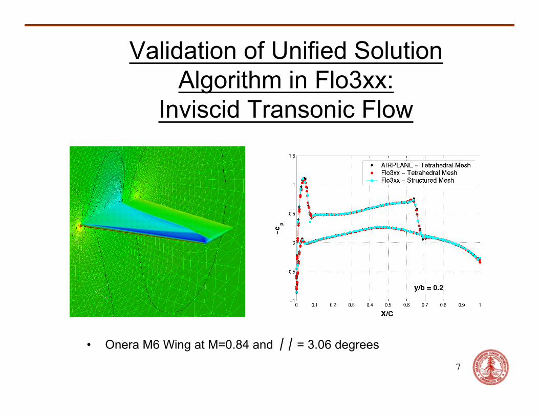
Validation of Unified SolutionAlgorithm in Flo3xx:

Inviscid Transonic Flow

• Onera M6 Wing at M=0.84 and = 3.06 degrees

†

a

8

Convergence Using Automatic Multigrid

Engineering Accuracy

9

Initial Validation for Viscous Flow:Zero-Pressure-Gradient Boundary Layer

10

RANS Results Using FLO107-MBFor Drag Prediction Workshop

• Accurate drag prediction for complex geometries in transonic flow is still very hard

• Flo3xx is currently in viscous validation phase.

• FLO107-MB has been thoroughly validated.

• Results of right figure were obtained with CUSP scheme and k- turbulence model

Statistical Evaluation DPW1 – All Participants Flo107-MB (DPW2)

†

w

11

Flo3xx Payoffs

• Highly flexible platform for all applied aerodynamics problems andother problems governed by conservation laws

• Fast turnaround through convergence acceleration techniques

• Framework can be used to support advanced research, such asthe BGK method or the Time-Spectral Method, which will beaddressed in this talk

• This means, take advanced research out of a laboratory settingand apply it to problems of practical engineering interest, which isultimately the only way to make an impact on the state-of-the art

Non LinearSymmetric Gauss-Seidel

Multigrid Scheme

Jameson + Caughey 2001Evolved from LUSGS scheme

Yoon + Jameson (1986)Rieger + Jameson (1986)

Achieved “Text Book” Multigrid Convergence

13

Nonlinear Symmetric Gauss-Seidel (SGS)Scheme

†

Forward and reverse sweeps :

For 1D case : ∂w∂t

+∂∂x

f w( ) = 0

Sweep (1) : Increasing j

w j1( ) = w j

0( ) - A -1 fj +

12

00( ) - fj- 1

2

10( )Ê

Ë Á

ˆ

¯ ˜

fj- 1

2

01( ) = f w j0( ),w j-1

1( )( )

A =∂f∂w

Sweep (2) : Decreasing j

w j2( ) = w j

1( ) - A -1 fj +

12

12( ) - fj- 1

2

11( )Ê

Ë Á

ˆ

¯ ˜

4 Flux evaluations in each double sweepCost per iteration similar to 4 - stage Runge - Kutta scheme

j

xx x xx

f f(10) (00)

w w w w w(1) (1) (0) (0) (0)

j

xx x xx

f f(11) (12)

w w w w w(1) (1) (1) (2) (2)

14

Solution of Burgers Equation on 131,072 Cellsin Two Steps With 15 Levels of Multigrid

0

9

10

8

7

6

5

4

3

2

1

Converged

15

Solution of 2D Euler Equations:Convergence for NACA0012

• The convergence history shows the successive computation on meshes ofdifferent sizes

• The convergence rate is independent of the mesh size• Convergence rate ~ .75 per cycle

16

Solution after 3 multigrid cycles

Solution of 2D Euler EquationsNACA0012 Airfoil

Solution after 5 multigrid cycles

Solid lines: fully converged result

17

Face-based Gauss Seidel (FBGS) Scheme

• On an arbitrary grid, loop over faces instead of looping over cells• Update the cells adjacent to a face as you go along• Updated state will be used on next visit to a cell

(Following a suggestion by John Vassberg)

18

The Finite-Volume BGK Scheme

Using Statistical Mechanics to EnhanceComputational Aerodynamics

Balaji SrinivasanGeorg May

Antony Jameson

19

A Major Conceptual DifferenceBetween Continuum Mechanics and

Statistical Mechanics

†

U = u f (x, y,z,u,v,w,x,t)Ú dudvdwdx

• In continuum mechanics the unknown solution variablesare defined “pointwise” with precise values:

†

U = U(x, y,z,t)• In statistical mechanics the solution variables exist only

as moments of a statistical distribution in physical andphase space, or as “expectation values”:

20

The Key Idea of the Finite-VolumeBGK Scheme

• Compute the fluxes for the Navier-Stokes equations atinterface N from the distribution functions in cells Aand B

• A time-dependent distribution function needs to beconstructed at each time step for each cell

21

Finding the Distribution Function

• The equilibrium distribution function

is known from Boltzmann statistics:

{ }2222 )()()(),,(),,(),,,,,,( xlx +-+-+--== wWvVuUzyxeq ezyxAwvuzyxgf

• The nonequilibrium distribution function

is unknown, but its evolution is given by the Boltzmann equation:

• Global numerical solution infeasible, because of highdimensionality

†

∂f∂t

+ u ∂f∂x

+ v ∂f∂y

+ w ∂f∂z

= Q( f , f ) CollisionIntegral

22

A Crucial Simplification(Bhatnagar, Gross & Krook - BGK)

• Replace the Collision Integral Q with a linear relaxation term:

†

Q = -f - g

t

†

∂f∂t

+ u∂f∂x

+ v ∂f∂y

+ w ∂f∂z

= -f - g

t

†

fi

• This equation can be solved analytically:

†

f ( r x , r u ,t,x) = g( r x - r u (t - ¢ t ), r u , ¢ t ,x)e-( t- ¢ t )

t d ¢ t + e-

tt f0( r x - r u t, r u ,x)

0

t

Ú

CollisionTime

23

A Key Observation

• By Chapman-Enskog expansion the Navier Stokes equations canbe recovered from the BGK equation, with the viscosity coefficient

†

m = t p• By setting the collision time appropriately, Navier-Stokes fluxes

can be computed directly from the distribution function

†

t

24

Payoff

• It is not necessary to compute the rate of strain tensor in order to calculateviscous fluxes

• This eliminates the need to perform two levels of numerical differentiation,which is difficult on arbitrary meshes

• Improved accuracy and reduced sensitivity to the quality of the mesh

• Automatic upwinding via the kinetic model, with no need for explicitartificial diffusion, thus reduced computational complexity

25

Viscous Validation of the BGK Scheme:Zero-Pressure-Gradient Boundary Layer

Velocity Profile (Incompressible) Temperature Profile (Compressible)

26

Viscous Validation of the BGK Scheme:1D Shock Structure (M=10)

Velocity Heat Flux

27

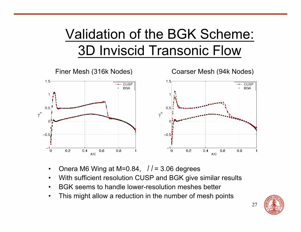
Validation of the BGK Scheme:3D Inviscid Transonic Flow

• Onera M6 Wing at M=0.84, = 3.06 degrees• With sufficient resolution CUSP and BGK give similar results• BGK seems to handle lower-resolution meshes better• This might allow a reduction in the number of mesh points

Finer Mesh (316k Nodes) Coarser Mesh (94k Nodes)

†

a

28

• Falcon Business Jet• M = 0.8• Angle of Attack: 2 degrees

Validation of the BGK Scheme usingFlo3xx:

3D Inviscid Transonic FlowDensity from 0.625 to 1.1

Fast Time Integration Methodsfor

Unsteady Problems

Arathi GopinathMatt McMullen

Antony Jameson

30

Potential Applications

• Flutter Analysis,

• Flow past Helicopter blades,

• Rotor-Stator Combinations in Turbomachinery,

• Zero-Mass Synthetic Jets for Flow Control

31

Dual Time Stepping BDFThe kth-order accurate backward difference formula (BDF) is of the form

where

The non-linear BDF is solved by inner iterations which advance in pseudo-time t*

The second-order BDF solves

Implementation via• RK “dual time stepping” scheme with variable local (RK-BDF)• Nonlinear SGS “dual time stepping” scheme (SGS-BDF)with Multigrid

†

dwdt* +

3w - 4wn + wn-1

2Dt+ R(w)

È

Î Í

˘

˚ ˙ = 0

†

Dt*

†

Dt =1Dt

1qq=1

k

 (D-)q

†

D-wn +1 = wn +1 - wn

32

Pressure Contours at Various Time Instances (AGARD 702)

Results of SGS-BDF Scheme(36 time steps per pitching cycle,3 iterations per time step )

12.36 millionReynolds Number

0.202Reduced Freq.

+/- 1.01deg.Pitching amplitude

0.796Mach Number

Test Case: NACA64A010pitching airfoil (CT6 Case)

Cycling to limit cycle

33

Payoff of Dual-time Stepping BDF Schemes

• Accurate simulations with an order of magnitude reduction in timesteps.

• For the pitching airfoil:

from ~ 1000 to 36 time steps per pitching cycle

with three sub-iterations in each step.

34

Frequency Domain and GlobalSpace-Time Multigrid Spectral

Methods

Application : Time-periodic flows

Using a Fourier representation in time, the time period T is divided

into N steps.

Then,

The discretization operator is given by

†

ˆ w k =1N

wn

n= 0

N-1

 e-iknDt

†

Dtwn =

2pT

ik ˆ w keiknDt

k=-N2

N2

-1

Â

35

Method 1 (McMullen et.al.) : Transform the equations into frequencydomain and solve them in pseudo-time t*

Method 2 (Gopinath et.al.) : Solve the equations in the time-domain.The space-time spectral discretization operator is

This is a central difference operator connecting all time levels,

yielding an integrated space-time formulation which requires

simultaneous solution of the equations at all time levels.

†

d ˆ w kdt* +

2pT

ik ˆ w k + ˆ R k = 0

†

Dtwn = dmwn +m

m=-N2

+1

N2

-1

 ,

†

dm =2pT

12

(-1)m +1 cot(pmN

),m ≠ 0

36

Comparison with Experimental Data -CL vs. a (CT6 Case)

RANS Time-Spectral Solution with 4, 8 and 12 intervals per pitching cycle

Computed Results

ExperimentalData

37

3D Test CaseNLR LANN Pitching Wing - RANS

.

6.28 millionReynolds Number

0.133Red. Frequency

62% RChordPitching axis

0.25degPitching Amplitude

0.59degMean Alpha

0.621Mach number

Pressure Contours on the Wing

CL vs. a plot with 4 and 8 time intervals

38

Application : Vertical-Axis WindTurbine(VAWT)

.Objective : To maximize power output of the VAWT by turbine blade redesign and various parametric studies.

39

VAWT : NACA0015 AirfoilSingle-Blade Inviscid 3D model

.

8Turbine Radius /

Blade Chord

5Blade Tip-Speed / V_inf

0.1Free-stream

Mach Number

Coefficient of Power generated bythe VAWT as a function of Rotation Angle - Time Spectral Method with 4,8 and 16 time intervals

40

• Engineering accuracy with very small number of time intervalsand same rate of convergence as the BDF.

• Spectral accuracy for sufficiently smooth solutions.

• Periodic solutions directly without the need to evolve through 5-10 cycles, yielding an order of magnitude reduction in computingcost beyond the reduction already achieved with the BDF,

for a total of two orders of magnitude.

Payoff of Time Spectral Schemes

41

Filtering the Navier-Stokes Equationswith

an Invertible Filter

42

Consider the incompressible Navier--Stokes equations

where

In large eddy simulation (LES) the solution is filtered to remove the small scales.Typically one sets

where the kernel G is concentrated in a band defined by the filter width. Then thefiltered equations contain the extra virtual stress

because the filtered value of a product is not equal to the product of the filteredvalues. This stress has to be modeled.

†

r∂ui

∂t+ ru j

∂ui

∂x j

+ r∂p∂xi

= m∂ 2ui

∂xi∂x j

(1)

†

∂ui

∂xi

= 0

†

u i (x) = G(x - ¢ x )u( ¢ x )dÚ ¢ x (2)

†

t ij = uiu j - ui u j (3)

43

A filter which completely cuts off the small scales or the high frequencycomponents is not invertible. The use, on the other hand, of an invertiblefilter would allow equation (1) to be directly expressed in terms of thefiltered quantities. Thus one can identify desirable properties of a filter as

1. Attenuation of small scales2. Commutativity with the differential operator3. Invertibility

†

Suppose the filter has the form ui = Pui (4)which can be inverted as Qui = ui (5)where Q = P-1. Moreover Q should be coercieve, so that Qu > c u (6)for some positive constant c.

44

†

Note that if Q commutes with ∂∂xi

then so does Q-1, since for any quantity f which is

sufficiently differentiable ∂∂xi

(Q-1 f ) = Q-1Q ∂∂xi

(Q-1 f )

= Q-1 ∂∂xi

(QQ-1 f )

= Q-1 ∂∂xi

( f )

Also since Q commutes with ∂∂xi

,

∂u∂xi

= 0 (7)

As an example P can be the inverse Helmholtz operator, so that one can write

Qui = 1-a 2 ∂ 2

∂xk∂xk

Ê

Ë Á

ˆ

¯ ˜ ui = ui (8)

where a is a length scale proportional to the largest scales to be retained. One may also introduce a filtered pressure p, satisfying the equation

Qp = 1-a 2 ∂ 2

∂xk∂xk

Ê

Ë Á

ˆ

¯ ˜ p = p (9)

45

†

Now one can substitute equation (8) and(9) for ui and p in equation (1) to get

r∂∂t

1-a 2 ∂ 2

∂xk∂xk

Ê

Ë Á

ˆ

¯ ˜ ui + r 1-a 2 ∂ 2

∂xk∂xk

Ê

Ë Á

ˆ

¯ ˜ u j

∂∂x j

1-a 2 ∂ 2

∂xl∂xl

Ê

Ë Á

ˆ

¯ ˜ ui +

∂∂xi

1-a 2 ∂ 2

∂xk∂xk

Ê

Ë Á

ˆ

¯ ˜ p

= m∂ 2

∂x j∂x j

1-a 2 ∂ 2

∂xk∂xk

Ê

Ë Á

ˆ

¯ ˜ ui

Because the order of the differentiations can be interchanged and the Helmholtz operator satisfies condition(6), it can be removed. The product term can be written as

r ∂∂x j

1-a 2 ∂ 2

∂xk∂xk

Ê

Ë Á

ˆ

¯ ˜ ui 1-a 2 ∂ 2

∂xl∂xl

Ê

Ë Á

ˆ

¯ ˜ u j

Ï Ì Ó

¸ ˝ ˛

= r∂

∂x j

ui u j -a 2 ui∂ 2 u j

∂xk∂xk

-a 2 u j∂ 2 ui

∂xk∂xk

+ a 4 ∂ 2 ui

∂xk∂xk

∂ 2 u j

∂xl∂xl

Ï Ì Ó

¸ ˝ ˛

= r∂

∂x j

ui u j -a 2 ∂ 2

∂xk∂xk

ui u j( ) + 2a 2 ∂ui

∂xk

∂u j

∂xk

+ a 4 ∂ 2 ui

∂xk∂xk

∂ 2 u j

∂xl∂xl

Ï Ì Ó

¸ ˝ ˛

= rQ ∂∂x j

ui u j + a 2Q-1 2∂ui

∂xk

∂u j

∂xk

+ a 2 ∂ 2 ui

∂xk∂xk

∂ 2 u j

∂xl∂xl

Ê

Ë Á

ˆ

¯ ˜

Ï Ì Ó

¸ ˝ ˛

According to condition (6), if Qf = 0 for any sufficiently differentiable quantity f , then f = 0.

46†

Thus the filtered equation finally reduces to

r ∂ui

∂t+ r

∂∂x j

ui u j( ) +∂ p∂xi

= m∂ 2 ui

∂xk∂xk

- r∂

∂x j

t ij (10)

with the virtual stress

t ij = a 2Q-1 2∂ui

∂xk

∂u j

∂xk

+ a 2 ∂ 2 ui

∂xk∂xk

∂ 2 u j

∂xl∂xl

Ê

Ë Á

ˆ

¯ ˜ (11)

The virtual stress may be calculated by solving

1-a 2 ∂ 2

∂xk∂xk

Ê

Ë Á

ˆ

¯ ˜ t ij = a 2 2∂ui

∂xk

∂u j

∂xk

+ a 2 ∂ 2 ui

∂xk∂xk

∂ 2 u j

∂xl∂xl

Ê

Ë Á

ˆ

¯ ˜ (12)

Taking the divergence of equation (10), it also follows that p satisfies the Poisson equation

∂ 2 p∂xi∂xi

+ r∂

∂xi

∂∂x j

ui u j( ) + r∂ 2

∂xi∂x j

t ij = 0 (13)

47

†

In a discrete solution scales smaller than the mesh width would not be resolved, amountingto an implicit cut off. There is the possibility of introducing an explicit cut off off in t ij . Also one could use equation (8) to restore an estimate of the unfiltered velocity.

In order to avoid solving the Helmholtz equation (12), the inverse Helmholtz operator could be expanded formally as

1-a 2D( )-1=1+ a 2D + a 4D2 + ...

where D denotes the Laplacian ∂ 2

∂xk∂xk

.Now retaining terms up to the fourth power of a,

the approximate virtual stress tensor assumes the form

t ij = 2a 2 ∂ui

∂xk

∂u j

∂xk

+ a 4 2D∂ui

∂xk

∂u j

∂xk

Ê

Ë Á

ˆ

¯ ˜ + DuiDu j

È

Î Í

˘

˚ ˙ (14)

One may regard the forms (11) or (14) as prototypes for subgrid scale (SGS) models.

48†

The inverse Helmholtz operator cuts off the smaller scales quite gradually. One could design filters with a sharper cut off by shaping their frequency response. Denote the Fourier transform of f as

ˆ f = Ffwhere (in one space dimension)

ˆ f (k) =12p

f (x)e- ikxdx-•

•

Ú

f (k) =12p

ˆ f (k)e- ikxdk-•

•

Ú

Then the general form of an invertible filter is

F PfŸ

= S(k) ˆ f (k)

F QfŸ

=1

S(k)ˆ f (k)

where S(k) should decrease rapidly beyond a cut off wave number inversely proportional toa length scale a .

49

†

In the case of a general filter with inverse Q, the virtual stress follows from the relation Quiu j = uiu j = Qu iQu j

Then t ij = uiu j - u iu j = Q-1(Qu iQu j - Q(u iu j ))

This formula provides the form for a family of subgrid-scale models.